HAL Id: hal-00850756https://hal.archives-ouvertes.fr/hal-00850756

Submitted on 8 Aug 2013

HAL is a multi-disciplinary open accessarchive for the deposit and dissemination of sci-entific research documents, whether they are pub-lished or not. The documents may come fromteaching and research institutions in France orabroad, or from public or private research centers.

L’archive ouverte pluridisciplinaire HAL, estdestinée au dépôt et à la diffusion de documentsscientifiques de niveau recherche, publiés ou non,émanant des établissements d’enseignement et derecherche français ou étrangers, des laboratoirespublics ou privés.

Modelling strong seismic ground motion:three-dimensional loading path versus wavefield

polarizationMaria Paola Santisi d’Avila, Luca Lenti, Jean-François Semblat

To cite this version:Maria Paola Santisi d’Avila, Luca Lenti, Jean-François Semblat. Modelling strong seismic ground mo-tion: three-dimensional loading path versus wavefield polarization. Geophysical Journal International,Oxford University Press (OUP), 2012, 190 (3), pp.1607-1624. �10.1111/j.1365-246X.2012.05599.x�.�hal-00850756�

MODELING STRONG SEISMIC GROUND MOTION:

3D LOADING PATH VS WAVEFIELD POLARIZATION

Maria Paola Santisi d’Avila1, Luca Lenti

2 and Jean-François Semblat

2

1 Université Pierre et Marie Curie, IJLRDA, 75005 Paris, France. Email: paola.santisi_d_avila@upmc.fr

2 Université Paris Est, IFSTTAR, 75015 Paris, France.

Accepted date. Received date; in original form date

Abbreviate title: Modeling 1D-3C strong seismic ground motion

Corresponding author:

Maria Paola Santisi d’Avila

Université Pierre et Marie Curie

Institut Jean Le Rond D’Alembert

Address:

2, Rue du Pot de Fer

75005 Paris

France

Phone: +33 (0)1 44278708

Fax: +33 (0)1 44275259

Email: paola.santisi_d_avila@upmc.fr

mpaolasantisi@gmail.com

SUMMARY

Seismic waves due to strong earthquakes propagating in surficial soil layers may both reduce soil

stiffness and increase the energy dissipation into the soil. In order to investigate seismic wave

amplification in such cases, past studies have been devoted to one-directional shear wave

propagation in a soil column (1D-propagation) considering one motion component only (1C-

polarization). Three independent purely 1C computations may be performed (“1D-1C” approach)

and directly superimposed in the case of weak motions (linear behavior). The present research aims

at studying local site effects by considering seismic wave propagation in a 1D soil profile

accounting for the influence of the 3D loading path and nonlinear hysteretic behavior of the soil. In

the proposed “1D-3C” approach, the three components (3C-polarization) of the incident wave are

simultaneously propagated into a horizontal multilayered soil. A 3D nonlinear constitutive relation

for the soil is implemented in the framework of the Finite Element Method in the time domain. The

complex rheology of soils is modeled by mean of a multi-surface cyclic plasticity model of the

Masing-Prandtl-Ishlinskii-Iwan type. The great advantage of this choice is that the only data needed

to describe the model is the modulus reduction curve. A parametric study is carried out to

characterize the changes in the seismic motion of the surficial layers due to both incident wavefield

properties and soil nonlinearities. The numerical simulations show a seismic response depending on

several parameters such as polarization of seismic waves, material elastic and dynamic properties,

as well as on the impedance contrast between layers and frequency content and oscillatory character

of the input motion. The 3D loading path due to the 3C-polarization leads to multiaxial stress

interaction that reduces soil strength and increases nonlinear effects. The nonlinear behavior of the

soil may have beneficial or detrimental effects on the seismic response at the free surface,

depending on the energy dissipation rate. Free surface time histories, stress-strain hysteresis loops

and in-depth profiles of octahedral stress and strain are estimated for each soil column. The

combination of three separate 1D-1C nonlinear analyses is compared to the proposed 1D-3C

approach, evidencing the influence of the 3C-polarization and the 3D loading path on strong

seismic motions.

Key words: Strong motion; Site effects; Wave polarization; Nonlinear constitutive law; Finite

Element Method.

1 INTRODUCTION

Numerous seismic records show that the local site condition is one of the dominant factors

controlling the variation in ground motion and determination of the site-specific seismic hazard.

Soils are complex materials and a linear approach is not reliable to model their seismic response to

strong quakes. The evidence of nonlinear soil behavior comes from experimental cyclic tests on soil

samples, for different strain amplitudes, where it is observed departure from the linear state as well

as hysteresis when ground deformations up to around 0.01‰ are attained (Hardin & Drnevich

1972a; Hardin & Drnevich 1972b; Vucetic 1990). The nonlinearity is particularly manifested in

shear modulus reduction and in the increase of damping for increasing strain levels. The effect on

the transfer function of such nonlinear effects is a shift of the fundamental frequency toward lower

frequencies, as well as an attenuation of the spectral amplitudes at high frequencies (Beresnev &

Wen 1996). For places where recorded data are not available, but soil parameters are known, it is

necessary to estimate theoretically the transfer function based on the parameters of the soil layers.

One-directional wave propagation analyses are an easy way to estimate the free surface ground

motion, used as input signal in the design of structures. Schnabel et al. (1972) introduced the

equivalent-linear analysis as a way to approximate the computation of nonlinear site response

through an iterative procedure. In their method, the resulting shear modulus reduction and

increasing damping are independent of the stress-strain path (Kramer 1996). Nevertheless, the

popularity of the equivalent linear method is perhaps due to the small number of parameters needed,

its ease of use and its rapidity compared to time domain wave propagation. The equivalent linear

approach has been implemented into widely used codes, such as SHAKE (Schnabel et al. 1972) and

EERA (Bardet et al. 2000) to investigate one-component ground response of horizontally layered

sites. This method is assumed to be reasonable for strain levels between 0.01‰ and 1‰ (Ishihara

1996; Yoshida & Iai 1998). A complete nonlinear site response analysis with the incorporation of

hysteresis appears to be fundamental to investigate local seismic effects for high strain levels.

Furthermore, the three motion components are coupled due to the nonlinear behavior; they can not

be computed separately.

A complete nonlinear analysis requires the propagation of a seismic wave in a nonlinear medium by

integrating the wave equation in the time domain and using an appropriate constitutive model.

Inputs to these analyses include acceleration time histories at bedrock and nonlinear material

properties of the various soil strata underlying the site. The main difficulty in nonlinear analysis is

to find a constitutive model that reproduces faithfully the nonlinear and hysteretic behavior of soil

under cyclic loadings, with the minimum number of parameters. Realistic hysteretic behavior of

soils is difficult to model because the yield surface may have a complex form. Some researchers

adopt the theory of plasticity to describe the hysteresis of soil (Zienkiewicz et al. 1982; Chen &

Baladi 1985; Chen & Mizuno 1990; Prevost & Popescu 1996; Ransamooj & Alwash 1997;

Montans 2000); others propose simplified nonlinear models (Kausel & Assimaki 2002; Delépine et

al. 2009) and other ones combine elasto-plastic constitutive equations with empirical rules (Ishihara

& Towhata 1982; Finn 1982; Towhata & Ishihara 1985; Iai et al. 1990a; Iai et al. 1990b; Kimura et

al. 1993). Classical empirical rules that describe the loading and unloading paths in the stress-strain

space are the so-called Masing rules, presented in 1926, (Kramer 1996), that reproduce quite

faithfully the hysteresis observed in the laboratory (Vucetic 1990). The main problem of these rules

is that the computed stress may exceed the maximum strength of the material when an irregular load

is applied (Pyke 1979; Li & Liao 1993). Several attempts have been done in order to overcome this

difficulty (Pyke 1979; Vucetic 1990; Bonilla, 2000).

The nonlinear site response analysis allows following the time evolution of the stress and strain

during seismic events and the resulting free surface ground motion. One-directional models for site

response analysis are proposed by several authors (Joyner & Chen 1975; Joyner et al. 1981, Lee &

Finn 1978; Pyke 1979; Bonilla, 2000; Hartzell S. et al. 2004; Phillips & Hashash 2009).

Furthermore, Li (1990) incorporates the three-dimensional cyclic plasticity soil model proposed by

Wang et al. (1990) in a finite element procedure, in terms of effective stress, to simulate the one-

directional wave propagation. However, this complex rheology needs an excessive number of

parameters to characterize the soil model.

The nonlinear rheology used in the present research is a multi-surface cyclic plasticity mechanism

that depends on few parameters that can be obtained from simple laboratory tests (Iwan 1967).

Material properties include the dynamic shear modulus at low strain and the variation of shear

modulus with shear strain. This rheology allows the dry soil to develop large strains in the range of

stable nonlinearity. Because of its three-directional nature, the procedure can handle both shear

wave and compression wave simultaneously and predict not only horizontal motion but vertical

settlement too. Iwan’s model is also called Masing-Prandtl-Ishlinskii-Iwan (MPII) model, according

to Segalman & Starr (2008). Two years later Masing’s postulate, in 1926, Prandtl proposed an

elasto-plastic model with strain-hardening, re-examined by Ishlinskii in 1944, obtained by coupling

a family of stops in parallel or of plays in series (Bertotti & Mayergoyz 2006). Segalman & Starr

(2008) showed that for any material behavior which may described as a Masing model, there exists

a unique parallel-series (strain based) Iwan system that provides forces as a function of the

displacement history. The MPII formulation of soil hysteretic behavior can be used to examine case

histories of well known stratigraphies as well as to investigate the role of critical parameters

affecting the soil response.

In the present research, a finite element procedure to evaluate stratified level ground response to

three-directional earthquakes is presented and the importance of the three-directional shaking

problem is analyzed. The main feature of the procedure is that it solves the specific three-

dimensional stress-strain problem with a one-directional approach.

The proposed “1D-3C” approach is implemented in a code called SWAP_3C (Seismic Wave

Propagation - 3 Components). The implementation of the nonlinear cyclic constitutive model is

presented in Sections 2 and 3. The code is then corroborated by comparison with the nonlinear

finite difference code NERA (Bardet & Tobita 2001), for the unidirectional propagation of a one-

component shear wave (“1D-1C”). The reliability of the proposed model is assessed and similar

results are produced (Section 4). A parametric analysis is developed to understand the influence of a

three-dimensional loading path and input polarization. The impact of a great vertical to horizontal

peak acceleration ratio is investigated. Effects of soil and input properties in the dynamic response

of soil columns are shown in Section 5. The conclusions are developed in Section 6.

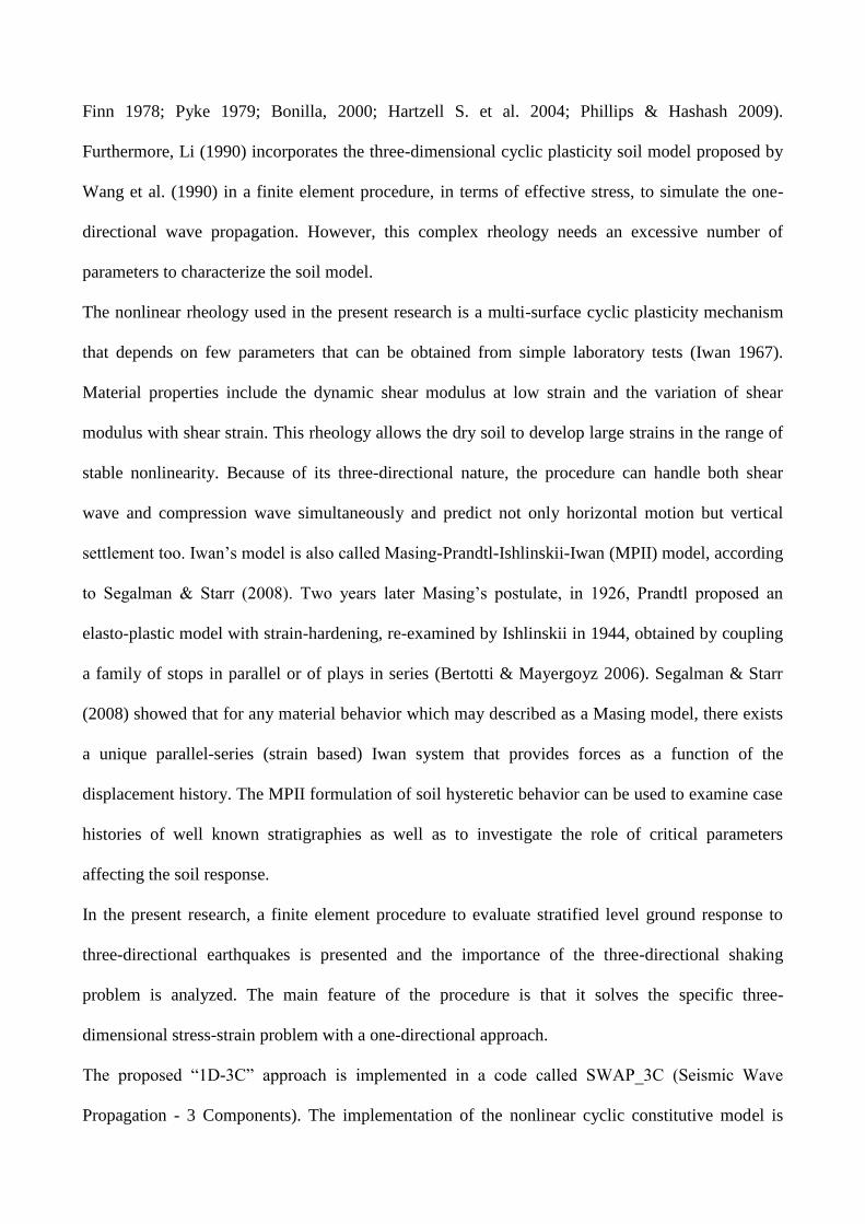
2 IMPLEMENTATION OF THE NONLINEAR CONSTITUTIVE MODEL

The three components of the seismic motion are propagated into a multilayered column of nonlinear

soil from the top of the underlying elastic bedrock, by using a finite element scheme. Along the

horizontal direction, at a given depth, soil is assumed here to be a continuous, homogeneous and

infinite medium. Soil stratification is discretized into a system of N horizontal layers, parallel to the

xy plane, using quadratic line elements with three nodes (Fig. 1). Shear and pressure waves

propagate vertically in z-direction. These hypotheses yield no strain variation in x- and y-direction.

Transformations remain small during the process and the cross sections of three-dimensional soil

elements remain planes.

According to a finite element modeling of a horizontally layered soil system, the strong form of

equilibrium equation in dynamic analysis, including compatibility conditions, three-dimensional

nonlinear constitutive relation and the imposed boundary conditions, is expressed in the matrix form

as

int M D CD F F&& & (1)

where M is the mass matrix, D& and D&& are velocity and acceleration vectors, respectively, i.e. the

first and second time derivatives of the displacement vector D . intF is the vector of nodal internal

forces and F is the load vector. C is a damping matrix derived from the fixed absorbing boundary

Figure1

condition, as explained below. The Finite Element Method, as applied in the present research, is

completely described in the works of Zienkiewicz (1971), Bathoz & Dhatt (1990), Reddy (1993)

and Cook et al. (2002).

Discretizing the soil column into en quadratic line elements and consequently into 2 1en n

nodes (Fig. 1), having three translational degrees of freedom each, yields a 3n -dimensional

displacement vector D composed by three blocks whose terms are the displacement of the n nodes

in x -, y - and z - direction, respectively. The assembled 3 3n n -dimensional mass matrix M

and the 3n -dimensional vector of internal forces intF result from the assemblage of 9 9 -

dimensional matrices like eM and vectors int

eF , respectively, corresponding to the element e , which

are expressed by

int0 0

e eh he T e T

e dz dz M N N F B σ (2)

where eh is the finite element length and e is the soil density assumed constant in the element. The

terms of the 6 -dimensional stress and strain vectors, defined as follows, are the independent stress

and strain components, respectively:

T

xx yy xy yz zx zz

T

xx yy xy yz zx zz

σ

ε (3)

where 0xx , 0yy and 0xy , according to the hypothesis of infinite horizontal soil. In

equation (2), zN is the 3 9 -dimensional shape function matrix. Integrals in equation (2) are

solved using the change of coordinates 1 2ez h with 2edz h d , where 1,1 is the

local coordinate in the element, and the Gaussian numerical integration. The shape function matrix

is defined, in local coordinates, as

1 2 3

1 2 3

1 2 3

N N N

N N N

N N N

N (4)

According to Cook et al. (2002), 1 1 2N , 2

2 1N and 3 1 2N are the

quadratic shape functions corresponding to the three-node line element used to discretize the soil

column. The terms of the 6 9 -dimensional matrix zB are the spatial derivatives of the shape

functions, according to compatibility conditions and to the hypothesis of no strain variation in the

horizontal directions x and y . If the strain vector is defined as ε u (Cook et al. 2002), where

the terms of u are the displacements in x -, y - and z -direction and is a matrix of differential

operators defined in such a way that compatibility equations are verified, matrix B N results

like

3 3 3 3 3

3 3 3 3 3

3 3 3 3 3

T

z

z

z

0 0 0 0 B 0

B 0 0 0 B 0 0

0 0 0 0 0 B

(5)

where 30 is a 3-dimensional null vector and 1 2 3

T

z N z N z N z B with

i iN z N z for 1,2,3i and 2 ez h .

The assemblage of 3 3n n -dimensional matrices and 3n -dimensional vectors is independently

done for each of the three n n -dimensional submatrices and n -dimensional subvectors,

respectively, corresponding to x -, y - and z -direction of motion.

The system of horizontal soil layers is bounded at the top by the free surface and at the bottom by a

semi-infinite elastic medium representing the seismic bedrock. The stresses normal to the free

surface are assumed null and the following condition, implemented by Joyner & Chen (1975) in a

finite difference formulation and used by Bardet & Tobita (2001) in NERA code, is applied at the

soil-bedrock interface to take into account the finite rigidity of the bedrock:

2T

b p σ c u u& & (6)

The stresses normal to the soil column base at the bedrock interface are T

p σ and c is a 3 3

diagonal matrix whose terms are b sbv , b sbv and b pbv . The parameters b , sbv and pbv are the

bedrock density and shear and pressure wave velocities in the bedrock, respectively. The three

terms of vector u& are the velocities in x -, y - and z -direction, respectively, at the interface soil-

bedrock (node 1 in Fig. 1). The terms of the 3 -dimensional vector bu& are the input velocities, in the

underlying elastic medium in directions x , y and z , respectively. The boundary condition (6)

allows energy to be radiated back into the underlying medium. According to equation (6), the

damping matrix 1C and the load vector 1

F , for the first element 1e , are defined by

1 11 1

0 02

h hT T

bdz dz C N c N F N c u& (7)

eC and eF are a null matrix and vector, respectively, for the other elements all over the soil profile.

The minimum number of quadratic line elements per layer j

en is defined considering that 10p is

the minimum number of nodes per wavelength to accurately represent the seismic signal

(Kuhlemeyer & Lysmer 1973; Semblat & Brioist 2000) and it is evaluated as

min2

jj

e

s

H p fn

v (8)

where jH is the thickness of layer j (Fig. 1), f is the frequency of the input signal and sv is the

assumed minimum shear velocity in the medium, corresponding to a 70% reduction of the initial

shear modulus. The seismic signal wavelength is equal to sv f .

The finite element model and the nonlinearity of soil require spatial and time discretization,

respectively, to permit the problem solution. The rate type constitutive relation between stress and

strain is linearized at each time step. Accordingly, equation (1) is expressed as

i i i i

k k k k k M D C D K D F&& & (9)

where the subscript k indicates the time step kt and i the iteration of the problem solving process,

as explained below.

The stiffness matrix i

kK is obtained by assembling 9 9 -dimensional matrices as follows, with

respect to element e :

,

0

ehe i T i

k kk dz B E B (10)

The tangent constitutive (6x6) matrix i

kE is evaluated by the incremental constitutive relationship

given by

i i i

k k k σ E ε (11)

According to Joyner (1975), the actual strain level and the strain and stress values at the previous

time step allow to evaluate the tangent constitutive matrix i

kE and the stress increment

1 1, ,i i i

k k k k k σ σ ε ε σ .

The step-by-step process is solved by the Newmark algorithm, expressed as follows:

1 1

1 12

12

1 1 1

2

i i

k k k k

i i

k k k k

tt

t t

D D D D

D D D D

& & &&

&& & &&

(12)

The Newmark procedure is a second-order approach for time integration in dynamic problems. The

two parameters 0.3025 and 0.6 guarantee a conditional numerical stability of the time

integration scheme (Hughes 1987). Equations (9) and (12) yield

1

i i

k k k k K D F A (13)

where the modified stiffness matrix is defined as

2

1i i

k kt t

K M C K (14)

and 1kA is a vector depending on the response in previous time step, given by

1 1 1

1 11

2 2k k kt

t

A M C D M C D& && (15)

Equation (9) requires an iterative solving, at each time step k , to correct the tangent stiffness matrix

i

kK . Starting from the stiffness matrix 1

1k kK K , evaluated at the previous time step, the value of

matrix i

kK is updated at each iteration i (Crisfield 1991). After evaluating the displacement

increment i

kD by equation (13), using the tangent stiffness matrix corresponding to the previous

time step, velocity and acceleration increments can be estimated through equation (12) and the total

motion is obtained according to

1 1 1

i i i i i i

k k k k k k k k k D D D D D D D D D& & & && && && (16)

where i

kD , i

kD& and i

kD&& are the vectors of total displacement, velocity and acceleration,

respectively. The strain increment i

kε is then derived from the displacement increment i

kD . The

stress increment i

kσ and tangent constitutive matrix i

kE are obtained through the constitutive

relationship (11), according to the MPII approach. Gravity load is imposed as static initial condition

in terms of strain and stress in nodes. The modified stiffness matrix i

kK is calculated and the

process restarts. The correction process continues until the difference between two successive

approximations is reduced to a fixed tolerance, according to

1i i i

k k k

D D D (17)

where 310 (Mestat 1993; Mestat 1998). Afterwards, the next time step is analyzed.

The one-dimensional three-component propagation model (“1D-3C” approach) proposed in this

Section is implemented in a code called SWAP_3C (Seismic Wave Propagation - 3 Components).

3 FEATURES OF THE CONSTITUTIVE MODEL

Modeling the propagation of a three-component earthquake in stratified soils requires a three-

dimensional constitutive model for soil. The so-called Masing-Prandtl-Ishlinskii-Iwan (MPII)

constitutive model, as suggested by Iwan (1967) and applied by Joyner (1975) and Joyner & Chen

(1975) in a finite difference formulation, is used in the present work to properly model the nonlinear

soil behavior in a finite element scheme. The MPII model is used to represent the behavior of

materials satisfying Masing criterion (Kramer 1996) and not depending on the number of loading

cycles. The stress level depends on the strain increment and strain history but not on the strain rate.

Therefore, this rheological model has no viscous damping. The energy dissipation process is purely

hysteretic and does not depend on the frequency. Iwan (1967) proposed an extension of the standard

incremental theory of plasticity (Fung 1965), by introducing a family of yield surfaces, modifying

the 1D approach with a single yield surface in stress space. He models nonlinear stress-strain curves

using a series of mechanical elements, having different stiffness and increasing sliding resistance.

The MPII model takes into account the nonlinear hysteretic behavior of soils in a three-dimensional

stress state, using an elasto-plastic approach with hardening, based on the definition of a series of

nested yield surfaces, according to von Mises’ criterion. Shear modulus and damping ratio are

strain-dependent. The MPII hysteretic model for dry soils, used in the present research, is applied

for strains in the range of stable nonlinearity.

The main feature of the MPII rheological model is that the only necessary input data, to identify soil

properties in the applied constitutive model, is the shear modulus decay curve G versus shear

strain . The initial elastic shear modulus 2

0 sG v , measured at the elastic behavior range limit

0.001 ‰ (Fahey 1992), depends on the mass density and the shear wave velocity in the

medium sv . The P-wave modulus 2

pM v , depending on the pressure wave velocity in the

medium pv , characterizes the longitudinal behavior of soil. The p sv v ratio, evaluated by

2

2 1 1 2p sv v (18)

is a function of the Poisson’s ratio . This is a parameter of the constitutive behavior for multiaxial

load and of the interaction between components in the three-dimensional response.

In the present study the soil behavior is assumed adequately described by a hyperbolic stress-strain

curve (Konder & Zelasko 1963; Hardin & Drnevich 1972b). This assumption yields a normalized

shear modulus decay curve, used as input curve representing soil characteristics, expressed as

0 1 1 rG G (19)

where r is a reference shear strain provided by test data corresponding to an actual tangent shear

modulus equivalent to 50% of the initial shear modulus. The applied constitutive model (Iwan

1967; Joyner & Chen 1975; Joyner 1975) does not depend on the hyperbolic backbone curve. It

could incorporate also shear modulus decay curves obtained from laboratory dynamic tests on soil

samples.

The deviatoric constitutive matrix dE for a three-dimensional soil element is deduced according to

Joyner (1975). The total constitutive matrix E in equation (11), such that σ E ε , is evaluated

in the proposed method starting from dE , according to

d E ST E H T (20)

where

6 6 6

diag 3 3 0 0 0 3

diag 1 1 1 2 1 2 1 2 1

B B BK K K

S

H

T t t 0 0 0 t

(21)

1 3 1 3 0 0 0 1 3T

t and 60 is a 6-dimensional null vector. Vectors and matrices in

equation (21) are deduced according to the definition of stress and strain vectors in equation (3).

The equation (20) is derived considering that the constitutive matrix dE , obtained according to the

Iwan procedure, allows evaluating the vector of deviatoric stress increments s knowing the vector

of deviatoric strain increments e , according to

d s E e (22)

where the deviatoric strain vector is defined as

/ 2 / 2 / 2

T

xx yy xy yz zx zz m

T

xx m yy m xy yz zx zz m

e e e e e e

e e

e H ε ε

(23)

and it corresponds to the following deviatoric stress vector:

T

xx yy xy yz zx zz m

T

xx m yy m xy yz zx zz m

s s s s s s

s σ σ

(24)

The volumetric strain 3m xx yy zz corresponds to the mean stress

3m xx yy zz . The relationship between m and m (Joyner 1975), supposed as elastic,

depends on the Bulk modulus BK , according to

3m B mK (25)

The vectors of mean stress and strain are respectively defined by

0 0 0

0 0 0

T

m m m m m

T

m m m m

σ S ε

ε T ε (26)

Equation (22) corresponds to m d m σ σ E H ε ε , according to (23) and (24). The

equation (20) is consequently deduced according to (26) and (11).

The three-component ground motion is characterized by the modulus which is a unique scalar

parameter. Similarly, octahedral shear stress (respectively strain) is chosen to combine the three-

dimensional stress (respectively strain) components in a unique scalar parameter. It allows an

adequate comparison of the simultaneous propagation of the three motion components (1D-3C) and

the independent propagation of the three components (1D-1C) superposed a posteriori. The 1D-1C

approach is a good approximation in the case of low strains within the linear range (superposition

principle; Oppenheim et al. 1997). The effects of axial-shear stress interaction in multiaxial stress

states have to be taken into account for higher strain rates, in the nonlinear range. Stress and strain

rate in the one-dimensional (1D) soil profile due to the propagation of a three-component

earthquake are therefore expressed in the following analysis in terms of octahedral shear stress and

strain, respectively obtained by

2 2 2 2 2 2

2 2 2

16

3

12 6

3

oct xx yy yy zz zz xx xy yz zx

oct zz yz zx

(27)

according to the hypothesis of infinite horizontal soil 0, 0, 0xx yy xy .

4 ANALYSIS OF THE LOCAL 1D-1C SEISMIC RESPONSE

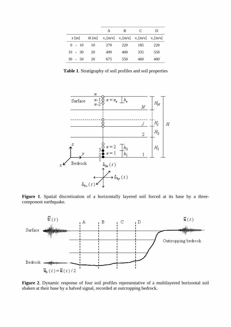
Four soil profiles are modeled in the present study consisting of three layers on seismic bedrock

(Fig. 2). The shear wave velocity profile of these soil columns is deduced using the approach

proposed by Cotton et al. (2006), based on the model of Boore & Joyner (1997). An average shear

wave velocity in the upper 30m 30sV of 350 - 300 - 250 m/s is assumed for columns A, B and C,

respectively. Soil column D has not an increasing shear velocity with depth but the middle layer is

the most rigid instead (Table 1).

The reference shear strain r of the hyperbolic model (equation (19)) is assumed equal to 0.35 - 0.5

- 1‰ in the various cases. The Poisson’s ratio is imposed equal to 0.3 - 0.4 - 0.45 to obtain different

values of the wave velocity ratio p sv v in the medium (1.87 - 2.45 - 3.32, respectively).

The physical properties assumed for the bedrock are the density 32100 /b kg m , the shear

velocity in the bedrock 1000 /sbv m s and the pressure wave velocity pbv is deduced by (18), by

imposing a Poisson’s ratio of 0.4.

The cyclic input signal used for the parametric analysis developed in the present research is the

following Mavroeidis-Papageorgiou wavelet (Semblat & Pecker 2009) with a phase shift:

max 2( ) 1 cos cos 2

2 2 2

f f

p

t tu fu t t f t

n

&&&& (28)

where maxu&& , f and f pt n f are the signal amplitude, fundamental frequency and duration,

respectively, and pn is the number of peaks that describes the oscillatory character of the motion.

Figure2

Table1

Such simple wavelets classically allow an easier verification for various amplitudes and number of

cycles. The interest of this specific wavelet (28) is justified in order to control both the predominant

frequency and the number of cycles. The latter is very important due to the influence of the loading

history. Various input signal parameters are chosen to assess their effects on the seismic ground

motion. Input frequency f is assumed equal to 2 - 3 - 5 - 7 Hz. The number of peaks pn in the time

history is chosen equal to 5 - 10 - 20. Acceleration signals are halved to take into account the free

surface effect and integrated, to obtain the corresponding input data in terms of vertically incident

velocities, before being forced at the base of the horizontally multilayered soil profile. Various input

polarizations are chosen assuming the acceleration component in z -direction zu&& equal to 0.1 - 0.7 -

0.8 - 0.9 times the acceleration component in x -direction xu&& and y xu u&& && for all cases.

In the case of the one-component input, the nonlinear site response in time domain obtained by the

proposed model is corroborated by comparison with output data acquired by the nonlinear code

NERA (Bardet & Tobita 2001). NERA is a 1D-1C ground response analysis software where the

one-component constitutive model suggested by Iwan (1967) is implemented in a finite difference

formulation, using the boundary condition proposed by Joyner & Chen (1975). A Mavroeidis-

Papageorgiou SH wavelet is considered with five peaks, 3Hzf and max 0.35gu && , where

2g 9.81m/s is the gravitational acceleration. The proposed “1D-3C” approach (SWAP_3C code)

is compared to NERA for a one-component input, propagated in the z -direction (Fig. 3). The

reference shear strain r = 0.5‰ is assumed uniform in the soil profile.

The one-directional dynamic response of the three multilayer soil columns A, B and C is analyzed

in terms of maximum stress zx and maximum strain zx profiles, hysteresis loop in the most

deformed layer and free surface smoothed acceleration time histories. In the case of 1C propagation,

the shear modulus decreases according to the shear modulus decay curve of the material. The stress-

strain curve during a loading is referred to a backbone curve (Fig. 3), determined knowing the shear

modulus decay curve. The obtained predictions are coherent with the evaluations obtained by

NERA, in terms of variation with depth of the maximum strain and stress, hysteresis loop and free

surface acceleration (Fig. 3). Unwanted high frequencies in acceleration time-histories, derived

from the numerical integration scheme, are suppressed by smoothing (Fig. 3c). Low-pass filtering

could be more suitable for real signals. Free surface accelerations obtained by NERA are not

altered.

5 PARAMETRIC ANALYSIS OF THE LOCAL 1D-3C SEISMIC RESPONSE

5.1 1D-3C vs 1D-1C approach

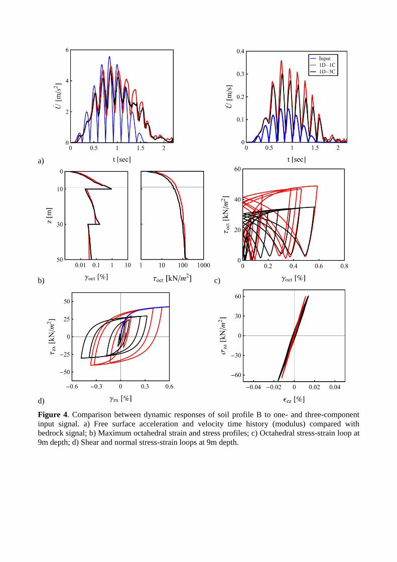
Modeling the propagation of a three-component earthquake in a soil column directly allows taking

into account the interactions between shear and pressure components of seismic load in a one-

directional seismic response analysis.

A cyclic signal is used to analyze nonlinear effects under a triaxial stress state. The dynamic

response of a soil column to the propagation of a three-component signal is compared to the

superposition of the three independently propagated components. Soil properties used in the

present analysis are shown in Table 1. An input signal with 3Hzf and five peaks is imposed at

the base of soil column B (Fig. 2). The reference shear strain r = 0.5‰ is assumed uniform in the

soil profile. The assumed PGA is equal to 0.35g for the two horizontal components and a ratio

0.8z xu u && && is assumed for the vertical component. The dynamic response of soil column B is

shown in Fig. 4.

Cyclic shear strains with amplitude greater than the elastic behavior range limit give open loops in

the shear stress-shear strain plane, exhibiting strong hysteresis. The shear modulus decreases and

the dissipation increases with increasing strain amplitude, due to nonlinear effects. The Fig. 4 shows

the soil column cyclic response in terms of shear stress and strain in x-direction, when both it is

affected by a triaxial input signal and the x-component of the input signal is independently

propagated. From one to three components, for a given maximum strain amplitude, the shear

Figure4

modulus decreases and the dissipation increases. Under triaxial loading the material strength is

lower than for simple shear loading referred to as the backbone curve. The compressive stiffness is

also reduced for multiaxial loading.

The dynamic response to a 3C signal is represented in terms of modulus for acceleration, velocity

and displacement time histories and in terms of octahedral parameters for stresses and strains. The

modulus of acceleration at the outcropping bedrock, with a peak max 0.57gu && , appears reduced at

the free surface of the analyzed soil column for both 1D-1C and 1D-3C approaches (Fig. 4).

Conversely, velocity modulus time histories are amplified. The interaction between multiaxial

stresses in the 3C approach yields a reduction of the ground motion at the free surface. Maximum

octahedral strain and stress profiles are obtained by (27) depending on profiles of maximum strains

zx , yz , zz and maximum stresses zx , yz , xx , yy , zz , respectively. Maximum strain and

stress components are not simultaneous in the analyzed time history. The hysteresis loops in terms

of octahedral strain and stress are obtained evaluating octahedral strain and stress time histories by

equations (27), knowing zx , yz , zz and zx , yz , xx , yy , zz , respectively, at each time step.

5.2 Influence of the soil properties

Average shear wave velocity

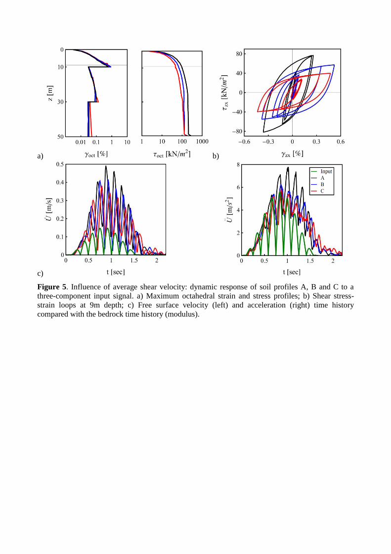
The 1D-3C dynamic response of columns A, B and C is compared in Fig. 5. The same input signal

with five peaks, 3Hzf , PGA equal to 0.35g for the two horizontal components and a ratio

0.8bz bxu u && && is used. A reference shear strain 1r ‰ and Poisson’s ratio 0.4 , assumed

uniform in soil columns A, B and C, have been chosen to minimize nonlinear effects induced by

lower r and Poisson’s ratio. The most rigid profile A shows the largest strength and lowest strains.

The opposite is obtained for the softest profile C. The free surface velocity is more amplified for the

rigid column A and the higher rate of energy dissipation in a softer soil yields lower amplification

in column C. The free surface acceleration is amplified in all analyzed soil columns, in this

particular case, compared with the assumed acceleration peak max 0.57gu && at the outcropping

bedrock (Fig. 5). Free surface velocity is similarly amplified.

Reference shear strain

Soil profile B is used to compare dynamic responses in the case of different reference shear strain

r equal to 0.35 - 0.5 - 1‰, assumed uniform in all layers, with a Poisson’s ratio 0.4 . The input

acceleration signal has five peaks, 3Hzf , _ max _ max 0.35gx yu u && && and 0.8z xu u && && . Nonlinear

effects starting at a lower strain rate yield lower strength (Fig. 6) and lower velocity amplification at

the free surface. An amplification of the acceleration signal is observed at the free surface for the

case of 1r ‰. The amplitude reduction is inversely related to the reference shear strain.

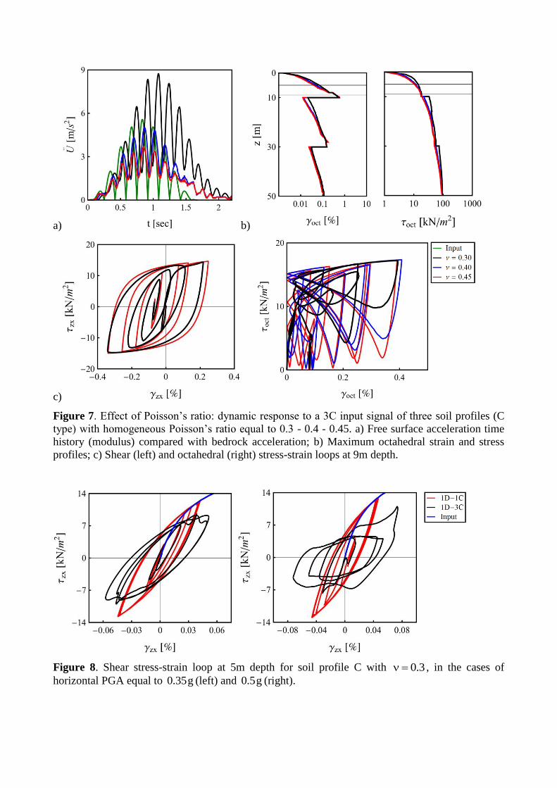
Poisson’s ratio

An important variation in the dynamic response of soil profiles is observed for different values of

the Poisson’s ratio. The softest soil profile C is analyzed assuming a Poisson’s ratio of 0.3 - 0.4 -

0.5 and a reference shear strain r = 0.35‰, both supposed uniform in the soil profile. A lower

value of yields a lower pressure to shear velocity ratio in the medium that causes greater signal

amplification and multiaxial stress interaction, shown in hysteresis loops (Fig. 7).

Free surface acceleration appears amplified, compared to the signal at outcropping bedrock, for

0.3 and reduced for analyzed cases with greater than 0.4 (Fig. 7). Velocity time history is

amplified in all investigated cases. The Fig. 7 shows a hysteresis loop in terms of shear stress and

strain in x -direction with more obvious nonlinear effects and three-component interaction in the

case of 0.3 , rather than for higher values of the p sv v ratio.

Shear stress-strain cycles at 5m depth in column C, with r = 0.35‰ and 0.3 , are shown in Fig.

8 for the cases of horizontal PGA _ maxxu&& equal to 0.35g (left) and 0.5g (right). The dynamic

Figure5

Figure6

Figure7

response in x -direction, influenced by the loading amplitude in directions y and z and by the

lower pressure to shear velocity ratio in the soil, is assessed by the 1D-3C approach and,

conversely, the 1D-1C scheme is not affected by the interaction of multiaxial stresses and strains.

The loop shape changes in each cycle and this interaction effect increases with the PGA. The 1D-

1C model does not permit to predict such change. The stress-strain cycles for each direction are

altered as a consequence of the coupling between loading components, according to Montans’

results (Montans 2000). This effect is more obvious for a low Poisson’s ratio and increases with

loading amplitude.

5.3 Seismic wave polarization and loading features

Polarization

The softest profile C is analyzed applying different input signals and comparing the dynamic

response. Reference shear strain r = 0.35‰ and Poisson’s ratio 0.4 are assumed uniform in the

soil profile. Soil column C is shaken by a three-component signal with equal component in x - and

y -direction, with _ max 0.35gxu && , 3Hzf and five peaks. The dynamic response to a signal with

different ratio between z - and x -component 0.1 0.7 0.8 0.9z xu u && && is shown in Fig. 9 to

investigate the influence of a high bedrock pressure wave.

Velocity amplification increases with the z xu u&& && ratio. The reduction of free surface acceleration,

compared to the signal at outcropping bedrock, is greatly lowered by the increasing z xu u&& && ratio. No

significant differences are obtained in terms of maximum shear stress. The loop shape changes with

increasing strain, as a consequence of the coupling between loading components, according to

Montans (2000). This effect is less important in this case, with 0.4 (Fig. 9 for 0.8z xu u && && ),

than for 0.3 (Fig. 8). The hysteresis loop in terms of octahedral strain and stress confirms a

three-component interaction effect with larger maximum octahedral strain and more obvious non

linear behavior.

Figure8

Figure9

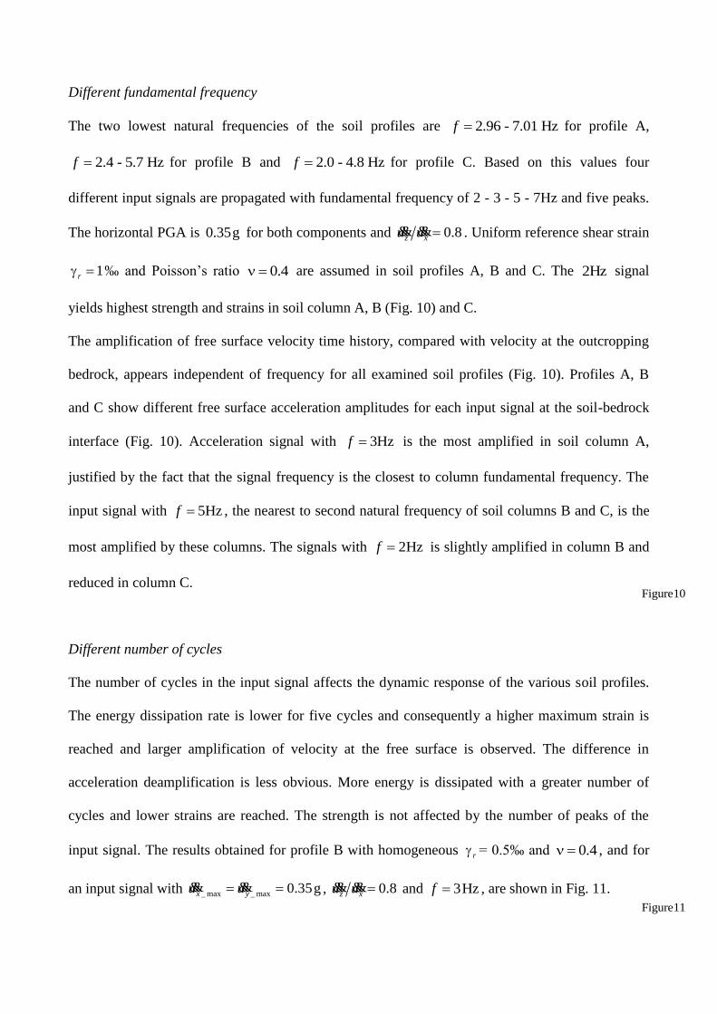
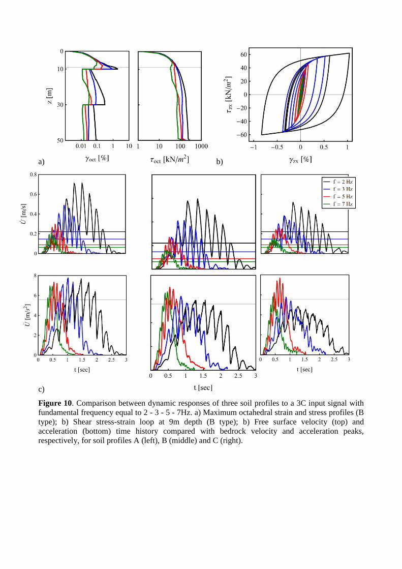
Different fundamental frequency

The two lowest natural frequencies of the soil profiles are 2.96 - 7.01 Hz f for profile A,

2.4 - 5.7 Hz f for profile B and 2.0 - 4.8 Hz f for profile C. Based on this values four

different input signals are propagated with fundamental frequency of 2 - 3 - 5 - 7Hz and five peaks.

The horizontal PGA is 0.35g for both components and 0.8z xu u && && . Uniform reference shear strain

1r ‰ and Poisson’s ratio 0.4 are assumed in soil profiles A, B and C. The 2Hz signal

yields highest strength and strains in soil column A, B (Fig. 10) and C.

The amplification of free surface velocity time history, compared with velocity at the outcropping

bedrock, appears independent of frequency for all examined soil profiles (Fig. 10). Profiles A, B

and C show different free surface acceleration amplitudes for each input signal at the soil-bedrock

interface (Fig. 10). Acceleration signal with 3Hzf is the most amplified in soil column A,

justified by the fact that the signal frequency is the closest to column fundamental frequency. The

input signal with 5Hzf , the nearest to second natural frequency of soil columns B and C, is the

most amplified by these columns. The signals with 2Hzf is slightly amplified in column B and

reduced in column C.

Different number of cycles

The number of cycles in the input signal affects the dynamic response of the various soil profiles.

The energy dissipation rate is lower for five cycles and consequently a higher maximum strain is

reached and larger amplification of velocity at the free surface is observed. The difference in

acceleration deamplification is less obvious. More energy is dissipated with a greater number of

cycles and lower strains are reached. The strength is not affected by the number of peaks of the

input signal. The results obtained for profile B with homogeneous r = 0.5‰ and 0.4 , and for

an input signal with _ max _ max 0.35gx yu u && && , 0.8z xu u && && and 3Hzf , are shown in Fig. 11.

Figure10

Figure11

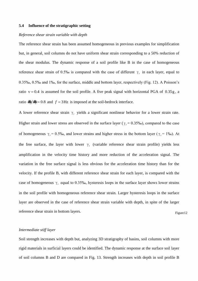
5.4 Influence of the stratigraphic setting

Reference shear strain variable with depth

The reference shear strain has been assumed homogeneous in previous examples for simplification

but, in general, soil columns do not have uniform shear strain corresponding to a 50% reduction of

the shear modulus. The dynamic response of a soil profile like B in the case of homogeneous

reference shear strain of 0.5‰ is compared with the case of different r in each layer, equal to

0.35‰, 0.5‰ and 1‰, for the surface, middle and bottom layer, respectively (Fig. 12). A Poisson’s

ratio 0.4 is assumed for the soil profile. A five peak signal with horizontal PGA of 0.35g , a

ratio 0.8z xu u && && and 3Hzf is imposed at the soil-bedrock interface.

A lower reference shear strain r yields a significant nonlinear behavior for a lower strain rate.

Higher strain and lower stress are observed in the surface layer ( r = 0.35‰), compared to the case

of homogeneous r = 0.5‰, and lower strains and higher stress in the bottom layer ( r = 1‰). At

the free surface, the layer with lower r (variable reference shear strain profile) yields less

amplification in the velocity time history and more reduction of the acceleration signal. The

variation in the free surface signal is less obvious for the acceleration time history than for the

velocity. If the profile B, with different reference shear strain for each layer, is compared with the

case of homogeneous r equal to 0.35‰, hysteresis loops in the surface layer shows lower strains

in the soil profile with homogeneous reference shear strain. Larger hysteresis loops in the surface

layer are observed in the case of reference shear strain variable with depth, in spite of the larger

reference shear strain in bottom layers.

Intermediate stiff layer

Soil strength increases with depth but, analyzing 3D stratigraphy of basins, soil columns with more

rigid materials in surficial layers could be identified. The dynamic response at the surface soil layer

of soil columns B and D are compared in Fig. 13. Strength increases with depth in soil profile B

Figure12

(Fig. 12, variable r curve). The effect of a more rigid middle soil layer (profile D) is analyzed.

A reference shear strain r equal to 0.35‰, 0.5‰ and 1‰ is assumed for the first, second and third

layer, respectively, with 0.4 for all layers. A five peak signal with horizontal PGA of 0.35g , a

ratio 0.8z xu u && && and 3Hzf is imposed at soil column base. Lower strains and unmodified

strength are observed in the surface layer of column D and higher strains and lower strength in the

bottom layer. Profiles A, B and C have the same trend when compared with D. The free surface

velocity and acceleration amplitude is slightly greater when the rigidity is not regularly increasing

with depth.

6 CONCLUSIONS

A geomechanical model is proposed to analyze the one-dimensional propagation of seismic waves

due to strong quakes and accounting for the three motion components (1D-3C approach). A finite

element modeling of horizontally layered soil is proposed, by adopting a three-dimensional

constitutive relation of the Masing-Prandtl-Ishlinskii-Iwan (MPII) type that needs few parameters to

characterize the hysteretic behavior of soils.

The proposed method provides a promising solution for strong seismic ground motion evaluation

and site effect analysis.

A parametric study is presented to evidence the effects of the input motion polarization and 3D

loading path analyzed by the “1D-3C” approach. The combination of three separate “1D-1C”

nonlinear analyses is compared to the proposed “1D-3C” approach.

Multiaxial stress states induce strength reduction of the material and larger damping effects. Soil

properties such as the upper limit of linear behavior range and the Poisson’s ratio have great impact

in local seismic response, influencing the soil dissipative properties. Input motion properties such as

polarization (vertical to horizontal component ratio), fundamental frequency and oscillatory

character (number of peaks) affect energy dissipation rate and thus the amplification effect. In

Figure13

particular, a low wave velocity ratio in the soil and a high vertical to horizontal component ratio

increase the three-dimensional mechanical interaction and progressively change the hysteresis loop

size and shape at each cycle.

The proposed model is verified by comparison with a finite difference unidirectional one-

component propagation model of the literature (NERA code). Validation of the “1D-3C” approach

against recorded free surface time histories should now be carried out. Local site effects in the

Tohoku area during the 2011 Tohoku earthquake are actually being investigated by the authors,

using the one-dimensional three-component propagation model proposed in this paper.

The MPII hysteretic model, used in the present research for dry soils, is applied for strains in the

range of stable nonlinearity. The extension of the proposed “1D-3C” approach to higher strain rates

is planned as further investigation to be able to study the effects of soil nonlinearity in drained

conditions.

The Finite Element Method efficiency when strong heterogeneities and complex geometries are

modeled allows an extension of the present approach to 2D and 3D alluvial basins but the amount

of data in both linear and nonlinear ranges would be huge.

AKNOWLEDGMENTS

The first author is very grateful to Prof. Mauro Schulz for his constructive suggestions. This work

was partly funded by the French National Research Agency (Quantitative Seismic Hazard

Assessment research project) and by the Radioprotection and Nuclear Safety Institute.

REFERENCES

Bardet J.P., Ichii K. & Lin C.H., 2000. EERA: A Computer Program for Equivalent-linear

Earthquake site Response Analyses of Layered Soil Deposits, University of Southern California,

United States.

Bardet J.P. & Tobita T., 2001. NERA: A Computer Program for Nonlinear Earthquake site

Response Analyses of Layered Soil Deposits, University of Southern California, United States.

Batoz J.L. & Dhatt G., 1990. Modélisation des structures par éléments finis, Vol. 1, ed. Hermes,

Paris, France.

Beresnev I.A. & Wen K.L., 1996. Nonlinear soil response. A reality?, Bull. Seism. Soc. Am., 86(6),

1964‒1978.

Bertotti G. & Mayergoyz I., 2006. The science of Hysteresis: Mathematical modeling and

applications, Elsevier, Amsterdam, Netherlands.

Bonilla L.F., 2000. Computation of linear and nonlinear site response for near field ground motion,

PhD thesis, University of California, Santa Barbara, United States.

Boore D.M. & Joyner W.B., 1997, Site amplifications for generic rock sites, Bull. Seism. Soc. Am.,

87(2), 327–341.

Chen W.F. & Baladi G.Y., 1985. Soil plasticity: theory and implementation, Elsevier Science

Publishers, New York, United States.

Chen W.F. & Mizuno E., 1990. Nonlinear analysis in soil mechanics: theory and implementation,

Elsevier Science Publishers, Amsterdam, Netherlands.

Cook R.D., Malkus D.S., Plesha M.E. & Witt R.J., 2002. Concepts and applications of finite

element analysis, 4th edn, John Wiley & Sons, New York, United States.

Cotton F., Scherbaum F., Bommer J.J. & Bungum H., 2006. Criteria for selecting and adjusting

ground-motion models for specific target regions: Application to Central Europe and rock sites, J.

Seismol., 10, 137‒156.

Crisfield M.A., 1991. Non-linear finite element analysis of solids and structures, Vol. 1, John Wiley

& Sons, Chichesrter, England.

Delépine N., Bonnet G ., Lenti L., Semblat J.F., 2009. Nonlinear viscoelastic wave propagation: an

extension of Nearly Constant Attenuation models, J. Eng. Mech., 135(11), 1305‒1314.

Fahey M., 1992. Shear modulus of cohesionless soil: variation with stress and strain level, Can.

Geotech. J., 29, 157‒161.

FinnW.D.L., 1982. Fundamental aspects of response of Tailing Dams to earthquakes, in Dynamic

Stability of Tailing Dams, ASCE National Convention, New Orleans, Louisiana.

Fung Y.C., 1965. Foundation of Soil Mechanics, Prentice Hall, Englewood Cliffs, New Jersey.

Hardin B.O. & Drnevich V.P., 1972a. Shear modulus and damping in soil: measurement and

parameter effects, J. Soil Mech. Found. Div., 98, 603‒624.

Hardin B.O. & Drnevich V.P., 1972b. Shear modulus and damping in soil: design equations and

curves, J. Soil Mech. Found. Div., 98, 667‒692.

Hartzell S., Bonilla L.F. & Williams R.A., 2004. Prediction of Nonlinear Soil Effects, Bull. Seism.

Soc. Am., 94(5), 1609‒1629.

Hughes T.J.R., 1987. The finite element method - Linear static and dynamic finite element analysis,

Prentice Hall, Englewood Cliffs, New Jersey.

Iai S., Matsunaga Y. & Kameoka T., 1990a. Strain space plasticity model for cyclic mobility, Rep.

Port Harbour Res. Inst., 29(4), 27‒56.

Iai S., Matsunaga Y. & Kameoka T., 1990b. Parameter identification for cyclic mobility model,

Rep. Port Harbour Res. Inst., 29(4), 57‒83.

Ishihara K., 1996. Soil behaviour in earthquake geotechnics, Clarenton Press, Oxford, England.

Ishihara K. & I. Towhata, 1982. Dynamic response analysis of level ground based on the effective

stress method, in Soil Mechanics - Transient and cyclic loads: constitutive relations and numerical

treatment, pp. 133‒172, ed. Pande G.N. & Zienkiewicz O.C., Wiley, John Wiley & Sons.

Iwan W.D., 1967. On a class of models for the yielding behavior of continuous and composite

systems, J. Appl. Mech., 34, 612‒617.

Joyner W., 1975. A method for calculating nonlinear seismic response in two dimensions, Bull.

Seism. Soc. Am., 65(5), 1315‒1336.

Joyner W.B. & Chen A.T.F., 1975. Calculation of nonlinear ground response in earthquakes, Bull.

Seism. Soc. Am., 65(5), 1315‒1336.

Joyner W.B., Warrick R.E. & Fumal T.E., 1981. The effect of quaternary alluvium on strong

ground motion in the Coyote Lake, California, earthquake of 1979, Bull. Seism. Soc. Am., 71(4),

1333‒1349.

Kausel E. & Assimaki D., 2002. Seismic simulation of inelastic soils via frequency-dependent

moduli and damping, J. Eng. Mech., 128(1), 34‒47.

Kimura T., Takemura J., Hirooka A., Ito K., Matsuda T. & Toriihara M., 1993. Numerical

prediction for Model N. , in Verification of numerical procedures for the analysis of soil

liquefaction problems, Vol. 1, pp. 141‒152, ed. Arulanandan and Scott, Rotterdam, Netherlands.

Konder R.L. & Zelasko J.S., 1963. A hyperbolic stress-strain formulation for sands, in Proc. 2nd

Pan American Conf. on Soil Mechanics and Foundations Engineering, pp. 289‒324, Brazil.

Kramer S. L., 1996. Geotechnical Earthquake Engineering, Prentice Hall, New Jersey.

Kuhlemeyer R.L. & Lysmer J., 1973. Finite element method accuracy for wave propagation

problems, J. Soil Mech. Found. Div., 99(SM5), 421‒427.

Lee K. W. & Finn W.D.L., 1978. DESRA-2: Dynamic effective stress response analysis of soil

deposits with energy transmitting boundary including assessment of liquefaction potential, Soil

Mechanics Series, University of British Columbia, Vancouver.

Li X.S., 1990. Free field response under multidirectional earthquake loading, PhD thesis, University

of California, Davis.

Li X. & Liao Z., 1993. Dynamic skeleton curve of soil stress-strain relation under irregular cyclic

loading, Earthquake Res. China, 7, 469‒477.

Li X.S., Wang Z.L. & Shen C.K., 1992. SUMDES: A nonlinear procedure for response analysis of

horizontally-layered sites subjected to multi-directional earthquake loading, University of

California, Davis.

Mestat P., 1993. Lois de comportement des géomatériaux et modélisation par la méthode des

éléments finis, in Etudes et recherches des Laboratoires des Ponts et Chaussées, Geotechnical

Series, GT52, Paris, France.

Mestat P., 1998. Modèles d’éléments finis et problèmes de convergence en comportement non

linéaire, Bull. Lab. Ponts Chaussées, 214, 45‒60.

Montans F.J., 2000. Bounding surface plasticity model with extended Masing behavior, Comput.

Meth. Appl. Mech. Eng., 182, 135‒162.

Oppenheim A.V., Willsky A.S. & Nawab S.H., 1997. Signals and Systems, 2nd edn, Prentice Hall.

Phillips C. & Hashash Y.M.A., 2009. Damping formulation for nonlinear 1D site response analyses,

Soil Dyn. Earthq. Eng., 29(7), 1143‒1158.

Prevost J.H. & Popescu R., 1996. Constitutive relations for soil materials, Electron. J. Geotech.

Eng., 1.

Pyke R., 1979. Nonlinear model for irregular cyclic loadings, J. Geotech. Eng. Div., 105, 715‒726.

Ramsamooj D. V. & Alwash A. J., 1997. Model prediction of cyclic response of soil, J. Geotech.

Eng., 116, 1053‒1072.

Reddy J. N., 1993. An introduction to the finite element method, 2nd edn, Mac Graw Hill.

Schnabel P.B., Lysmer J. & Seed H.B., 1972. SHAKE: A computer program for earthquake

response analysis of horizontally layered sites, Report UCB/EERC-72/12, Earthquake Engineering

Research Center, University of California, Berkeley, United States.

Segalman, D.J. & Starr, M. J., 2008. Inversion of Masing models via continuous Iwan systems, Int.

J. Nonlinear Mech., 43, 74‒80.

Semblat J.F. and Brioist J.J., 2000. Efficiency of higher order finite elements for the analysis of

seismic wave propagation, J. Sound Vibrat., 231(2), 460–467.

Semblat J.F. & Pecker A., 2009. Waves and vibrations in soils, IUSS Press, Pavia, Italy.

Towhata I. & K. Ishihara, 1985. Modeling soil behaviour under principal axes rotation, in Proc.

Fifth Intern. Conf. on Numerical methods in geomechanics, pp. 523‒530, Nagoya, Japan.

Vucetic M., 1990. Normalized behaviour of clay under irregular cyclic loading, Can. Geothech. J.,

27(1), 29‒46.

Wang Z. L., Dafalias Y.F. & Shen C.K., 1990. Bounding surface hypoelasticity model for sand, J.

Eng. Mech., 116(5), 983‒1001.

Yoshida N. & S. Iai, 1998. Nonlinear site response and its evaluation and prediction, in Proc.

Second Int. Symp. on the Effects of Surface Geology on Seismic Motion, Vol. 1, pp. 71‒90,

Netherlands.

Zienkiewicz O.C. 1971. La Méthode des Eléments Finis appliqué à l’art de l’ingénieur, translation

of G. Vouille (1973), Ediscience, France.

Zienkiewicz O.C., K. H. Leung, E. Hinton & C. T. Chang, 1982. Liquefaction and permanent

deformation under dynamic conditions - Numerical solution and constitutive relations, in Soil

Mechanics - Transient and cyclic loads: constitutive relations and numerical treatment, pp. 71‒104,

ed. Pande G.N. & Zienkiewicz O.C., John Wiley & Sons.

Figure 1. Spatial discretization of a horizontally layered soil forced at its base by a three-

component earthquake.

Figure 2. Dynamic response of four soil profiles representative of a multilayered horizontal soil

shaken at their base by a halved signal, recorded at outcropping bedrock.

Figure 3. Comparison between results obtained by the proposed “1D-3C” approach (SWAP_3C

code) and NERA for a one-component input in profiles A, B and C. a) Maximum strain (left) and

stress (right) profiles; b) Shear stress-strain loop at 41 m depth; c) Free surface acceleration time

history.

Figure 4. Comparison between dynamic responses of soil profile B to one- and three-component

input signal. a) Free surface acceleration and velocity time history (modulus) compared with

bedrock signal; b) Maximum octahedral strain and stress profiles; c) Octahedral stress-strain loop at

9m depth; d) Shear and normal stress-strain loops at 9m depth.

Figure 5. Influence of average shear velocity: dynamic response of soil profiles A, B and C to a

three-component input signal. a) Maximum octahedral strain and stress profiles; b) Shear stress-

strain loops at 9m depth; c) Free surface velocity (left) and acceleration (right) time history

compared with the bedrock time history (modulus).

Figure 6. Effect of the reference shear strain: dynamic response to a 3C input signal of three soil

profiles (B type) with homogeneous reference shear strain equal to 0.35 - 0.5 - 1‰. a) Free surface

acceleration time history (modulus) compared with the bedrock acceleration; b) Maximum

octahedral strain and stress profiles; c) Shear (left) and octahedral (right) stress-strain loops at 9m

depth.

Figure 7. Effect of Poisson’s ratio: dynamic response to a 3C input signal of three soil profiles (C

type) with homogeneous Poisson’s ratio equal to 0.3 - 0.4 - 0.45. a) Free surface acceleration time

history (modulus) compared with bedrock acceleration; b) Maximum octahedral strain and stress

profiles; c) Shear (left) and octahedral (right) stress-strain loops at 9m depth.

Figure 8. Shear stress-strain loop at 5m depth for soil profile C with 0.3 , in the cases of

horizontal PGA equal to 0.35g (left) and 0.5g (right).

Figure 9. Effect of seismic wave polarization: dynamic responses of soil profile C to a three-

component input signal with z xu u ratio equal to 0.1 - 0.7 - 0.8 - 0.9%. a) Free surface velocity

(left) and acceleration (right) time history compared with bedrock velocity and acceleration peaks,

respectively; b) Shear (left) and octahedral (right) stress-strain loops at 5m depth.

Figure 10. Comparison between dynamic responses of three soil profiles to a 3C input signal with

fundamental frequency equal to 2 - 3 - 5 - 7Hz. a) Maximum octahedral strain and stress profiles (B

type); b) Shear stress-strain loop at 9m depth (B type); b) Free surface velocity (top) and

acceleration (bottom) time history compared with bedrock velocity and acceleration peaks,

respectively, for soil profiles A (left), B (middle) and C (right).

Figure 11. Comparison between dynamic responses of soil profile B to a three-component input

signal with 5 - 10 - 20 cycles. a) Free surface velocity (left) and acceleration (right) signals

compared with bedrock velocity and acceleration peaks, respectively; b) Shear (left) and octahedral

(right) stress-strain loop at 9m depth.

Figure12. Comparison between the dynamic response to a three-component input signal of two soil

profiles (B type) with homogeneous and variable reference shear strain. a) Maximum octahedral

strain and stress profiles (left) and free surface acceleration time history compared with the bedrock

acceleration (right); b) Maximum octahedral strain and stress profiles (left) and shear stress-strain

loop at 9m depth (right).

Figure 13. Influence of a stiff middle layer: dynamic response to a three-component input signal of

soil profiles B and D with variable reference shear strain. a) Maximum octahedral strain and stress

profiles; b) Shear stress-strain loop at 9m depth.

Table 1. Stratigraphy of soil profiles and soil properties

A B C D

z [m] th [m] vs [m/s] vs [m/s] vs [m/s] vs [m/s]

0 - 10 10 270 220 185 220

10 - 30 20 490 400 335 550

30 - 50 20 675 550 460 400

Table 1. Stratigraphy of soil profiles and soil properties

Figure 1. Spatial discretization of a horizontally layered soil forced at its base by a three-

component earthquake.

Figure 2. Dynamic response of four soil profiles representative of a multilayered horizontal soil

shaken at their base by a halved signal, recorded at outcropping bedrock.

a)

b)

c)

Figure 3. Comparison between results obtained by the proposed “1D-3C” approach (SWAP_3C

code) and NERA for a one-component input in profiles A, B and C. a) Maximum strain (left) and

stress (right) profiles; b) Shear stress-strain loop at 41 m depth; c) Free surface acceleration time

history.

a)

b) c)

d)

Figure 4. Comparison between dynamic responses of soil profile B to one- and three-component

input signal. a) Free surface acceleration and velocity time history (modulus) compared with

bedrock signal; b) Maximum octahedral strain and stress profiles; c) Octahedral stress-strain loop at

9m depth; d) Shear and normal stress-strain loops at 9m depth.

a) b)

c)

Figure 5. Influence of average shear velocity: dynamic response of soil profiles A, B and C to a

three-component input signal. a) Maximum octahedral strain and stress profiles; b) Shear stress-

strain loops at 9m depth; c) Free surface velocity (left) and acceleration (right) time history

compared with the bedrock time history (modulus).

a) b)

c)

Figure 6. Effect of the reference shear strain: dynamic response to a 3C input signal of three soil

profiles (B type) with homogeneous reference shear strain equal to 0.35 - 0.5 - 1‰. a) Free surface

acceleration time history (modulus) compared with the bedrock acceleration; b) Maximum

octahedral strain and stress profiles; c) Shear (left) and octahedral (right) stress-strain loops at 9m

depth.

a) b)

c)

Figure 7. Effect of Poisson’s ratio: dynamic response to a 3C input signal of three soil profiles (C

type) with homogeneous Poisson’s ratio equal to 0.3 - 0.4 - 0.45. a) Free surface acceleration time

history (modulus) compared with bedrock acceleration; b) Maximum octahedral strain and stress

profiles; c) Shear (left) and octahedral (right) stress-strain loops at 9m depth.

Figure 8. Shear stress-strain loop at 5m depth for soil profile C with 0.3 , in the cases of

horizontal PGA equal to 0.35g (left) and 0.5g (right).

a)

b)

Figure 9. Effect of seismic wave polarization: dynamic responses of soil profile C to a three-

component input signal with z xu u ratio equal to 0.1 - 0.7 - 0.8 - 0.9%. a) Free surface velocity

(left) and acceleration (right) time history compared with bedrock velocity and acceleration peaks,

respectively; b) Shear (left) and octahedral (right) stress-strain loops at 5m depth.

a) b)

c)

Figure 10. Comparison between dynamic responses of three soil profiles to a 3C input signal with

fundamental frequency equal to 2 - 3 - 5 - 7Hz. a) Maximum octahedral strain and stress profiles (B

type); b) Shear stress-strain loop at 9m depth (B type); b) Free surface velocity (top) and

acceleration (bottom) time history compared with bedrock velocity and acceleration peaks,

respectively, for soil profiles A (left), B (middle) and C (right).

a)

b)

Figure 11. Comparison between dynamic responses of soil profile B to a three-component input

signal with 5 - 10 - 20 cycles. a) Free surface velocity (left) and acceleration (right) signals

compared with bedrock velocity and acceleration peaks, respectively; b) Shear (left) and octahedral

(right) stress-strain loop at 9m depth.

a)

b)

Figure12. Comparison between the dynamic response to a three-component input signal of two soil

profiles (B type) with homogeneous and variable reference shear strain. a) Maximum octahedral

strain and stress profiles (left) and free surface acceleration time history compared with the bedrock

acceleration (right); b) Maximum octahedral strain and stress profiles (left) and shear stress-strain

loop at 9m depth (right).

a) b)

Figure 13. Influence of a stiff middle layer: dynamic response to a three-component input signal of

soil profiles B and D with variable reference shear strain. a) Maximum octahedral strain and stress

profiles; b) Shear stress-strain loop at 9m depth.