Page 1
Modelling the Dynamics ofMass Capture
by
Timothy John Lahey
A thesispresented to the University of Waterloo
in fulfillment of thethesis requirement for the degree of
Doctor of Philosophyin
Systems Design Engineering
Waterloo, Ontario, Canada, 2013
©Timothy John Lahey 2013
Page 2
I hereby declare that I am the sole author of this thesis. This is a true copy of the thesis,including any required final revisions, as accepted by my examiners.
I understand that my thesis may be made electronically available to the public.
ii
Page 3
Abstract
This thesis presents an approach to modelling dynamic mass capture which is applied to anumber of system models. The models range from a simple 2D Euler-Bernoulli beam withpoint masses for the end-effector and target to a 3D Timoshenko beam model (includingtorsion) with rigid bodies for the end-effector and target. In addition, new models for torsion,as well as software to derive the finite element equations from first principles were developedto support the modelling. Results of the models are compared to a simple experiment asdone by Ben Rhody. Investigations of offset capture are done by simulation to show why onewould consider using a 3D model that includes torsion.
These problems have relevance to both terrestrial robots and to space based roboticsystems such as the manipulators on the International Space Station capturing payloads suchas the SpaceX Dragon capsule. One could increase production in an industrial environmentif industrial robots could pick up items without having to establish a zero relative velocitybetween the end effector and the item. To have a robot acquire its payload in this way wouldintroduce system dynamics that could lead to the necessity of modelling a previously ‘rigid’robot as flexible.
iii
Page 4
Acknowledgements
First and foremost, I’d like to thank my supervisor Glenn Heppler who provided valuableadvice and assistance throughout this process. I’d also like to thank Wayne Brodland for hisguidance on several occasions. Lastly, I’d like to thank Kristine Meier without whom I’d likelynever have finished this thesis.
iv
Page 5
Contents
List of Tables viii
List of Figures ix
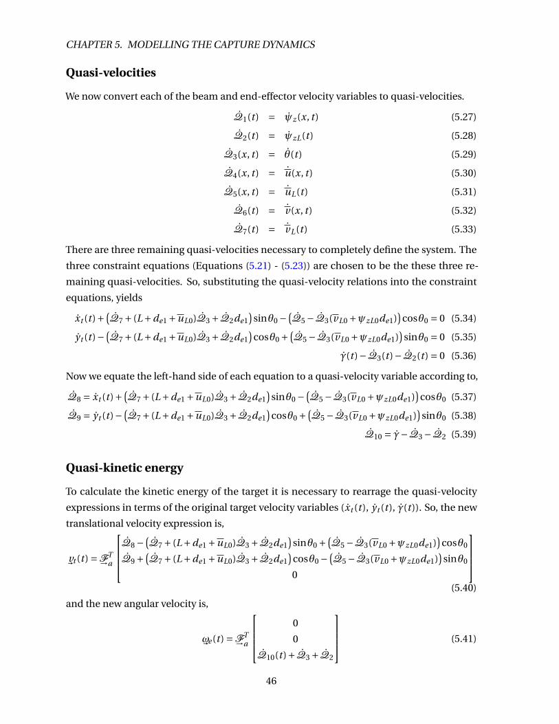
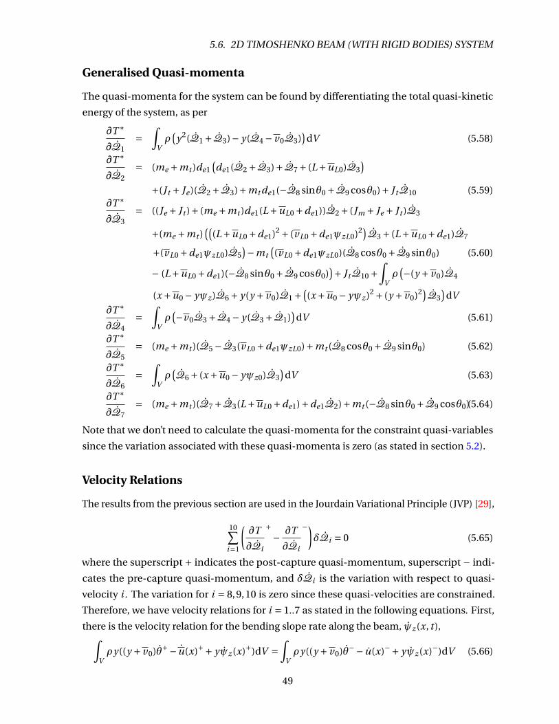
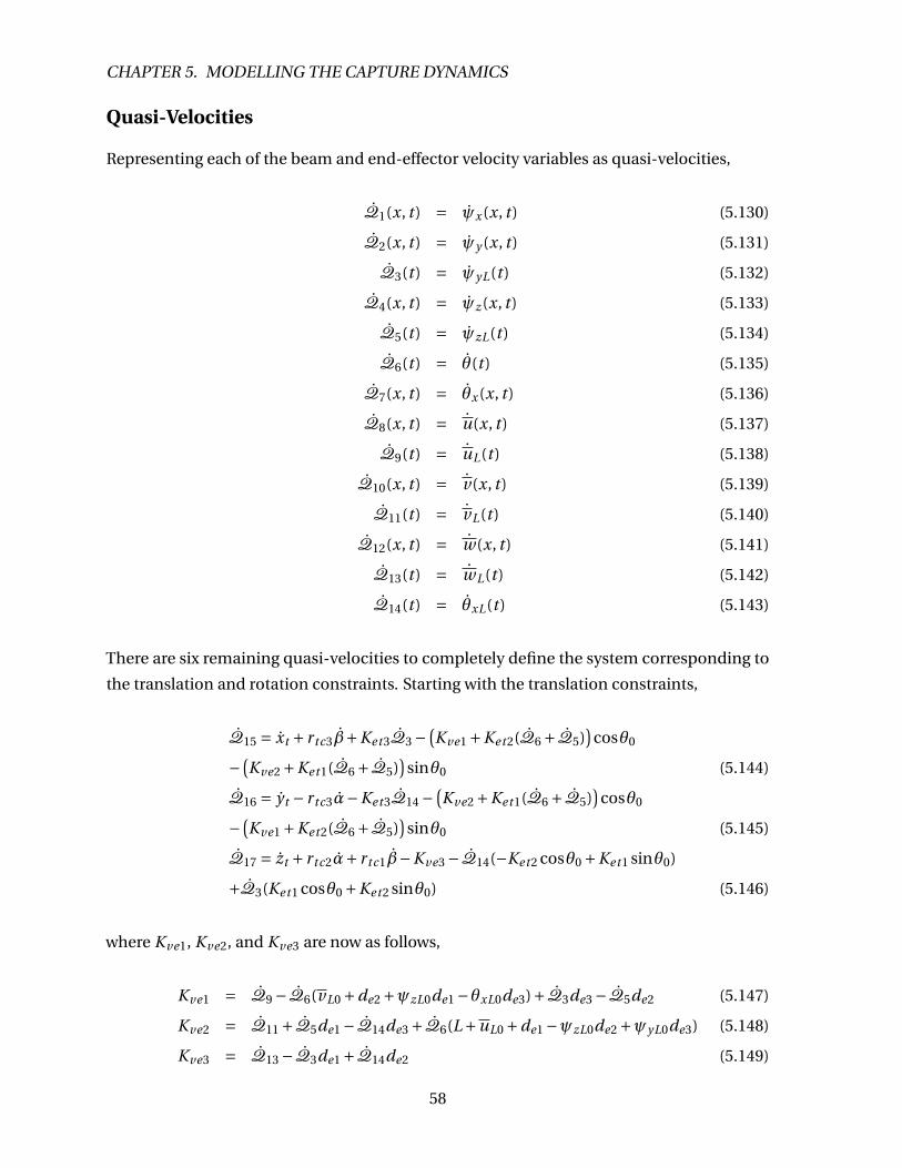
1 Introduction 11.1 Previous Work . . . . . . . . . . . . . . . . . . . . . . . . . . . . . . . . . . . . . 21.2 Layout of this document . . . . . . . . . . . . . . . . . . . . . . . . . . . . . . . 3
2 Beam Torsion Modelling 52.1 Overview . . . . . . . . . . . . . . . . . . . . . . . . . . . . . . . . . . . . . . . . 52.2 Traditional Torsion Models . . . . . . . . . . . . . . . . . . . . . . . . . . . . . . 82.3 Torsion Model Analysis . . . . . . . . . . . . . . . . . . . . . . . . . . . . . . . . 122.4 New Models for Torsion . . . . . . . . . . . . . . . . . . . . . . . . . . . . . . . . 14
3 System Work, Kinetic, and Potential Energy 183.1 Motor Work and Kinetic Energy . . . . . . . . . . . . . . . . . . . . . . . . . . . 193.2 Target Energy . . . . . . . . . . . . . . . . . . . . . . . . . . . . . . . . . . . . . . 193.3 Beam Energy . . . . . . . . . . . . . . . . . . . . . . . . . . . . . . . . . . . . . . 213.4 End-Effector Energy . . . . . . . . . . . . . . . . . . . . . . . . . . . . . . . . . . 26
4 Mixed Symbolic-Numeric Finite Element Modelling 324.1 Introduction . . . . . . . . . . . . . . . . . . . . . . . . . . . . . . . . . . . . . . 324.2 Overview . . . . . . . . . . . . . . . . . . . . . . . . . . . . . . . . . . . . . . . . 334.3 Assembly of Full Matrices . . . . . . . . . . . . . . . . . . . . . . . . . . . . . . . 354.4 Newmark-Beta Solver . . . . . . . . . . . . . . . . . . . . . . . . . . . . . . . . . 364.5 Pure Torsion Convergence Test . . . . . . . . . . . . . . . . . . . . . . . . . . . 37
5 Modelling the Capture Dynamics 405.1 Plastic Impact of Two Masses . . . . . . . . . . . . . . . . . . . . . . . . . . . . 405.2 Variational Methods for Mass Capture . . . . . . . . . . . . . . . . . . . . . . . 415.3 Analysis Process for Mass Capture Problems . . . . . . . . . . . . . . . . . . . 425.4 Capture Process Models . . . . . . . . . . . . . . . . . . . . . . . . . . . . . . . 43
v
Page 6
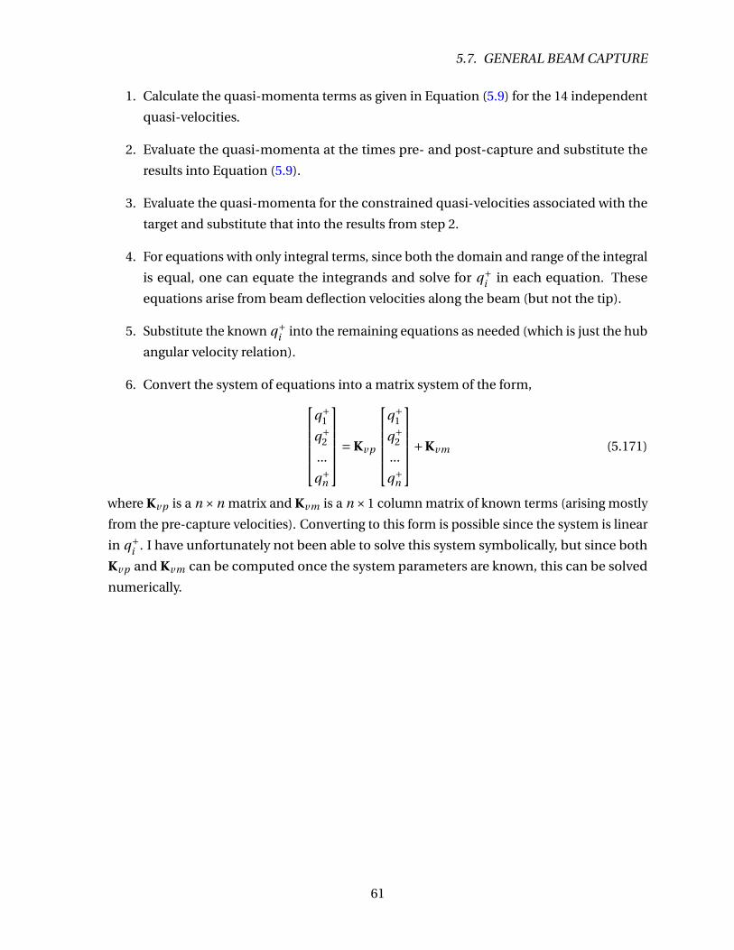
5.5 2D Euler-Bernoulli Beam (with Point Masses) System . . . . . . . . . . . . . . 435.6 2D Timoshenko Beam (with Rigid Bodies) System . . . . . . . . . . . . . . . . 445.7 General Beam Capture . . . . . . . . . . . . . . . . . . . . . . . . . . . . . . . . 54
6 Determination of System Damping 626.1 A Coupled System Approach to Damping Modelling . . . . . . . . . . . . . . . 646.2 Determining Transfer Functions . . . . . . . . . . . . . . . . . . . . . . . . . . . 646.3 Estimating ζ= f (ω) . . . . . . . . . . . . . . . . . . . . . . . . . . . . . . . . . . 726.4 Determining C through parameter identification . . . . . . . . . . . . . . . . . 746.5 Summary . . . . . . . . . . . . . . . . . . . . . . . . . . . . . . . . . . . . . . . . 76
7 Experiment, Results, and Discussion 777.1 Overview of Experiment . . . . . . . . . . . . . . . . . . . . . . . . . . . . . . . 777.2 Finite Element Models . . . . . . . . . . . . . . . . . . . . . . . . . . . . . . . . 797.3 Comparison of Natural Frequencies . . . . . . . . . . . . . . . . . . . . . . . . 827.4 2D Euler-Bernoulli Beam Results . . . . . . . . . . . . . . . . . . . . . . . . . . 887.5 2D Timoshenko Beam Model Results . . . . . . . . . . . . . . . . . . . . . . . . 967.6 3D Timoshenko Beam Model Results . . . . . . . . . . . . . . . . . . . . . . . . 1067.7 Investigation Of An Offset Capture . . . . . . . . . . . . . . . . . . . . . . . . . 1197.8 Discussion . . . . . . . . . . . . . . . . . . . . . . . . . . . . . . . . . . . . . . . 121
8 Discussion, Summary, Conclusions, and Future Work 1228.1 Discussion . . . . . . . . . . . . . . . . . . . . . . . . . . . . . . . . . . . . . . . 1228.2 Summary of Work . . . . . . . . . . . . . . . . . . . . . . . . . . . . . . . . . . . 1248.3 Conclusions . . . . . . . . . . . . . . . . . . . . . . . . . . . . . . . . . . . . . . . 1258.4 Future Work . . . . . . . . . . . . . . . . . . . . . . . . . . . . . . . . . . . . . . . 125
Appendices 127
A Torsion of Uniform Cross-section Beams 129A.1 Derivation of St. Venant Warping Function . . . . . . . . . . . . . . . . . . . . 129A.2 φ Dependence in Reissner Torsion . . . . . . . . . . . . . . . . . . . . . . . . . 154A.3 Modelling Torsion including Shear and Poisson Effects . . . . . . . . . . . . . 157
B Volume Integration of Variational Gradients 162
C Integration of φ over the cross-section 163C.1 Calculation of the P integral . . . . . . . . . . . . . . . . . . . . . . . . . . . . . 164C.2 Calculation of the K integral . . . . . . . . . . . . . . . . . . . . . . . . . . . . . 167C.3 Calculation of the Lc integral . . . . . . . . . . . . . . . . . . . . . . . . . . . . . 169C.4 Convergence analysis of the integrals . . . . . . . . . . . . . . . . . . . . . . . . 171
D Example use of Symbolic-Numeric Finite Element Package 178D.1 A Rotating 3D Timoshenko beam with a rigid body end-effector . . . . . . . . 178
E Jourdain’s Variational Principle and Impact 186
vi
Page 7
F Capture Dynamics of a 2D Euler-Bernoulli Beam 188F.1 Post-Capture Velocity Constraint . . . . . . . . . . . . . . . . . . . . . . . . . . 188F.2 Quasi-Velocities . . . . . . . . . . . . . . . . . . . . . . . . . . . . . . . . . . . . 189F.3 Quasi-Kinetic Energy . . . . . . . . . . . . . . . . . . . . . . . . . . . . . . . . . 189F.4 Generalised Quasi-Momenta . . . . . . . . . . . . . . . . . . . . . . . . . . . . . 191F.5 Velocity Relations . . . . . . . . . . . . . . . . . . . . . . . . . . . . . . . . . . . 191
Bibliography 195
Nomenclature 202
vii
Page 8
List of Tables
6.1 Natural Frequencies (Hz) [1] . . . . . . . . . . . . . . . . . . . . . . . . . . . . . . . 626.2 Damping Model Parameters . . . . . . . . . . . . . . . . . . . . . . . . . . . . . . . 72
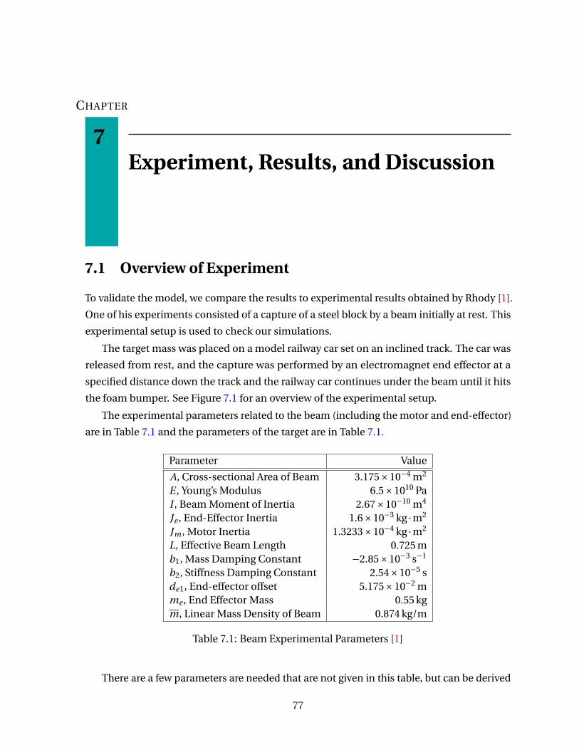
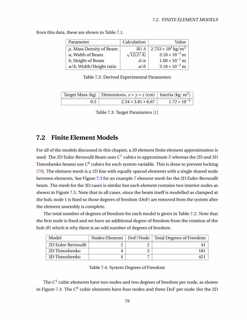
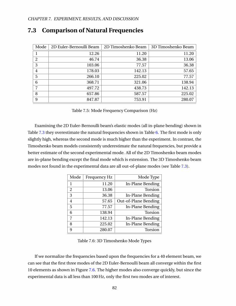
7.1 Beam Experimental Parameters [1] . . . . . . . . . . . . . . . . . . . . . . . . . . . 777.2 Derived Experimental Parameters . . . . . . . . . . . . . . . . . . . . . . . . . . . . 797.3 Target Parameters [1] . . . . . . . . . . . . . . . . . . . . . . . . . . . . . . . . . . . 797.4 System Degrees of Freedom . . . . . . . . . . . . . . . . . . . . . . . . . . . . . . . 797.5 Mode Frequency Comparison (Hz) . . . . . . . . . . . . . . . . . . . . . . . . . . . 827.6 3D Timoshenko Mode Types . . . . . . . . . . . . . . . . . . . . . . . . . . . . . . . 82
viii
Page 9
List of Figures
1.1 Simplified Model of Mass Capture . . . . . . . . . . . . . . . . . . . . . . . . . . . . 1
2.1 End-Effector Reference Frames . . . . . . . . . . . . . . . . . . . . . . . . . . . . . 62.2 Post-Capture Target and End-Effector Reference Frames . . . . . . . . . . . . . . 72.3 Arbitrary Cross-Section . . . . . . . . . . . . . . . . . . . . . . . . . . . . . . . . . . 10
3.1 2D System Model . . . . . . . . . . . . . . . . . . . . . . . . . . . . . . . . . . . . . . 183.2 2D System Model (with end-effector offset) . . . . . . . . . . . . . . . . . . . . . . 263.3 3D end-effector offset . . . . . . . . . . . . . . . . . . . . . . . . . . . . . . . . . . . 29
4.1 Element Matrix Calculation Process . . . . . . . . . . . . . . . . . . . . . . . . . . . 344.2 Pure Torsion Modes 1 through 4 Convergence . . . . . . . . . . . . . . . . . . . . . 384.3 Pure Torsion Modes 5 through 8 Convergence . . . . . . . . . . . . . . . . . . . . . 39
5.1 Two Particle Impact . . . . . . . . . . . . . . . . . . . . . . . . . . . . . . . . . . . . 415.2 3D Target Capture . . . . . . . . . . . . . . . . . . . . . . . . . . . . . . . . . . . . . 55
6.1 Empirical Transfer Function Estimate . . . . . . . . . . . . . . . . . . . . . . . . . 656.2 Modal Circle [2] . . . . . . . . . . . . . . . . . . . . . . . . . . . . . . . . . . . . . . . 666.3 Circle Fit Approximation for the first mode . . . . . . . . . . . . . . . . . . . . . . 696.4 Circle Fit Approximation for the second mode . . . . . . . . . . . . . . . . . . . . 706.5 Circle Fit Approximation for the rigid body mode . . . . . . . . . . . . . . . . . . . 716.6 Damping vs. Frequency (Various Approximations) . . . . . . . . . . . . . . . . . . 73
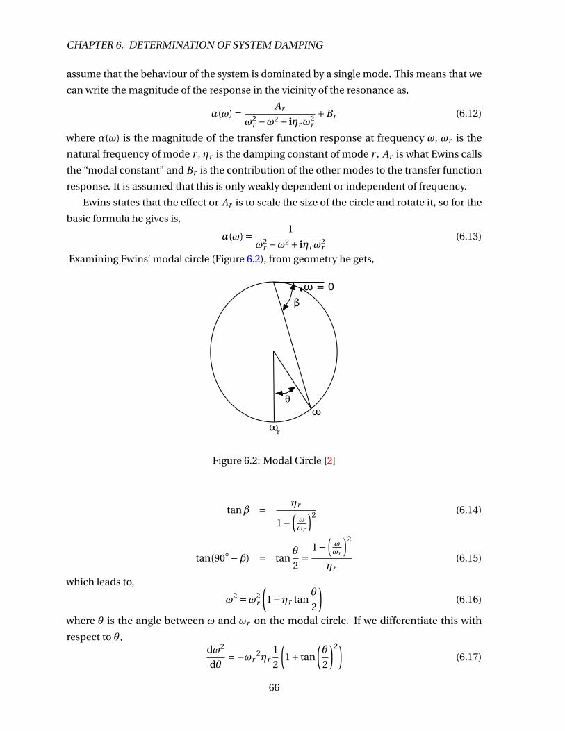
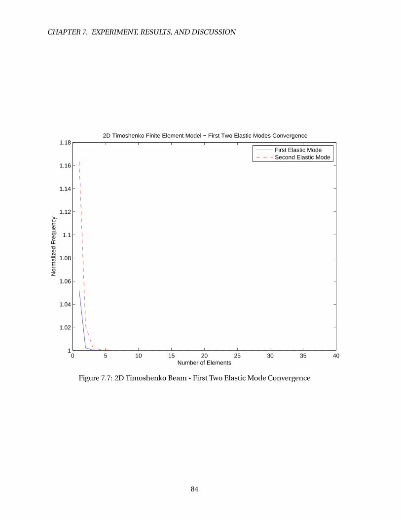
7.1 Experimental Setup - Side View [1] . . . . . . . . . . . . . . . . . . . . . . . . . . . 787.2 Experimental Setup - Beam Top View (Target Captured) . . . . . . . . . . . . . . . 787.3 2D Euler-Bernoulli Beam 7 Element Mesh . . . . . . . . . . . . . . . . . . . . . . . 807.4 2D Euler-Bernoulli C 1 Cubic Beam Element . . . . . . . . . . . . . . . . . . . . . . 807.5 3D Timoshenko C 0 Cubic Beam Element . . . . . . . . . . . . . . . . . . . . . . . . 817.6 2D Euler-Bernoulli Beam Elastic Mode Convergence . . . . . . . . . . . . . . . . . 837.7 2D Timoshenko Beam - First Two Elastic Mode Convergence . . . . . . . . . . . . 847.8 2D Timoshenko Beam Elastic Modes 3 through 6 Convergence . . . . . . . . . . . 85
ix
Page 10
7.9 3D Timoshenko Beam - First Four Elastic Modes Convergence . . . . . . . . . . . 867.10 3D Timoshenko Beam Elastic Modes 5 through 7 Convergence . . . . . . . . . . . 877.11 2D Euler-Bernoulli Beam Tip Deflection vs. Experiment . . . . . . . . . . . . . . . 887.12 2D Euler-Bernoulli Beam Tip Deflection vs. Experiment (initial 5s) . . . . . . . . 897.13 2D Euler-Bernoulli Beam FFT Simulation vs. Experiment . . . . . . . . . . . . . . 907.14 2D Euler-Bernoulli Beam Hub Rotation vs. Experiment (initial 0.15s) . . . . . . . 917.15 2D Euler-Bernoulli Beam Hub Rotation vs. Experiment . . . . . . . . . . . . . . . 927.16 2D Euler-Bernoulli Beam Hub Rotation vs. Experiment (initial 2.5s) . . . . . . . . 937.17 2D Euler-Bernoulli Beam Hub Rotation (Minimal Damping) . . . . . . . . . . . . 947.18 2D Euler-Bernoulli Beam Hub Rotation (Minimal Damping - Initial 1.2s) . . . . . 957.19 2D Timoshenko Beam Tip Deflection vs. Experiment . . . . . . . . . . . . . . . . 967.20 2D Timoshenko Beam Tip Deflection vs. Experiment (initial 5s) . . . . . . . . . . 977.21 2D Timoshenko Beam FFT Simulation vs. Experiment . . . . . . . . . . . . . . . . 987.22 2D Timoshenko Beam Hub Rotation vs. Experiment (initial 0.15s) . . . . . . . . . 997.23 2D Timoshenko Beam Hub Rotation vs. Experiment . . . . . . . . . . . . . . . . . 1007.24 2D Timoshenko Beam Hub Rotation vs. Experiment (initial 2.5s) . . . . . . . . . 1017.25 2D Timoshenko Beam Hub Rotation (Minimal Damping) . . . . . . . . . . . . . . 1027.26 2D Timoshenko Beam Hub Rotation (Minimal Damping - Initial 1.2s) . . . . . . 1037.27 2D Timoshenko Beam Tip Axial Deflection vs. Time . . . . . . . . . . . . . . . . . 1047.28 2D Timoshenko Beam Tip Rotation vs. Time . . . . . . . . . . . . . . . . . . . . . . 1057.29 3D Timoshenko Beam Tip Deflection vs. Experiment . . . . . . . . . . . . . . . . 1067.30 3D Timoshenko Beam Tip Deflection vs. Experiment (initial 5s) . . . . . . . . . . 1077.31 3D Timoshenko Beam FFT Simulation vs. Experiment . . . . . . . . . . . . . . . . 1087.32 3D Timoshenko Beam Hub Rotation vs. Experiment (initial 0.15s) . . . . . . . . . 1097.33 3D Timoshenko Beam Hub Rotation vs. Experiment . . . . . . . . . . . . . . . . . 1107.34 3D Timoshenko Beam Hub Rotation vs. Experiment (initial 2.5s) . . . . . . . . . 1117.35 3D Timoshenko Beam Hub Rotation (Minimal Damping) . . . . . . . . . . . . . . 1127.36 3D Timoshenko Beam Hub Rotation (Minimal Damping - Initial 1.2s) . . . . . . 1137.37 3D Timoshenko Beam Tip Axial Deflection vs. Time . . . . . . . . . . . . . . . . . 1147.38 3D Timoshenko Beam Tip In-Plane Rotation vs. Time . . . . . . . . . . . . . . . . 1157.39 3D Timoshenko Beam Tip Out-of-Plane Deflection vs. Time . . . . . . . . . . . . 1167.40 3D Timoshenko Beam Tip Out-of-Plane Rotation vs. Time . . . . . . . . . . . . . 1177.41 3D Timoshenko Beam Tip Angle of Twist vs. Time . . . . . . . . . . . . . . . . . . 1187.42 3D Timoshenko Beam Tip Angle of Twist vs. Time (1 mm z-offset) . . . . . . . . . 120
A.1 General Cross-Section Boundary Relations . . . . . . . . . . . . . . . . . . . . . . 132A.2 Rectangular Cross-section . . . . . . . . . . . . . . . . . . . . . . . . . . . . . . . . 133A.3 Series Contribution to J vs. N (β= 1) . . . . . . . . . . . . . . . . . . . . . . . . . . 152A.4 Comparing Approximation of the Series Contribution to J vs. N (β= 1) . . . . . . 153A.5 Series Contribution to J for β vs. N . . . . . . . . . . . . . . . . . . . . . . . . . . . 154
C.1 tanh vs. β (β from 1 to 5) . . . . . . . . . . . . . . . . . . . . . . . . . . . . . . . . . 172C.2 tanh vs. β (β from 2 to 4) . . . . . . . . . . . . . . . . . . . . . . . . . . . . . . . . . 173C.3 sech2 vs. β (β from 1 to 5) . . . . . . . . . . . . . . . . . . . . . . . . . . . . . . . . 174C.4 sech2 vs. β (β from 5 to 10) . . . . . . . . . . . . . . . . . . . . . . . . . . . . . . . . 175
x
Page 11
CHAPTER
1Introduction
This thesis details a project to model the dynamics of mass capture by a robotic link. Con-
tained in this thesis is an overview of previous related work and a discussion of the theory and
implementation various models of mass capture. In particular, this thesis contains models
where the end effector and target are modelled as a particle mass as well as models where
they are modelled as rigid bodies. The robot is modelled as a single flexible link driven by a
motor at its base (see Figure 1.1). The flexible link is modelled alternatively by a 2D Euler-
Bernoulli beam, a 2D Timoshenko beam, and a 3D Timoshenko beam (including torsion).
The simplified model of a particle mass target/end-effector (and a 2D Euler-Bernoulli beam)
is consistent with the model analysed by Kövecses et al. [3, 4] and the models from this thesis
are compared with their simplified model.
Oa
1
a2
mt
me
Figure 1.1: Simplified Model of Mass Capture
1
Page 12
CHAPTER 1. INTRODUCTION
1.1 Previous Work
The problem of having a flexible robot linkage acquire a moving payload, shall be referred to
as “dynamic mass capture”, and can be broken down into several sub-classes as follows.
Class I: a stationary linkage with a payload attached subjected to a non-plastic impact;
Class II: a stationary linkage with an end effector that captures a moving mass particle (plastic
impact);
Class III: a moving linkage with an end effector that captures a moving mass particle (known
trajectories);
Class IV: a stationary linkage with an end effector that captures a translating rigid body
(plastic impact);
Class V: a moving linkage with an end effector that captures a translating rigid body (plastic
impact);
Class VI: a stationary linkage with an end effector that captures a translating and spinning
rigid body (plastic impact);
Class VII: a moving linkage with an end effector that captures a translating and spinning rigid
body (plastic impact);
Class VIII: the capture of a translating and spinning rigid body which has moving internal
parts (e.g., momentum wheels).
These problems have relevance to both terrestrial robots and to space based robotic
systems such as the manipulators on the International Space Station. While the space
applications are relatively high profile the terrestrial applications have significant economic
implications. If industrial robots could pick up items without having to establish a zero
relative velocity between the end effector and the item, cycle time could be reduced. To have
a robot acquire its payload in this way would introduce system dynamics that could lead to
the necessity of modelling a previously ‘rigid’ robot as flexible.
The flexibility in robotic members has long been a topic of interest and the problem
that is the focus of this thesis has received attention [5]–[6]. It has most frequently been
modelled by using Bernoulli-Euler beam theory [7], but the Timoshenko beam theory has
better modelling fidelity in vibrations problems, especially for the higher modes [8].
To model the various cases of dynamic mass capture the impact dynamics of flexible
beams must be examined. Many dynamicists have investigated the flexible beam impact
problem for simply supported beams impacted in the centre [9, 10], but the proposed
research requires that the tip impact of a chain of flexible beams, connected by flexible joints
which also have friction and inertia must be studied. There has been work on the transverse
elastic impact at the tip of a two link rigid-flexible configuration [11], on the axial impact of a
single link [12, 13, 14], on the elastic impact on general rigid multibody systems [15, 16], on
2
Page 13
1.2. LAYOUT OF THIS DOCUMENT
the transverse elastic impact of single links [17, 18], and on the transverse plastic impact of
single links [19]. None of the cited references consider structural damping or anything but
ideal frictionless joints. Additional work related directly to spacecraft has also been reported
[5, 20, 6].
Chapnik et al. [21, 22] examined the impact of a sphere and a rotating flexible beam with
a tip mass, where the impact occurs at the tip mass (Class I). Of all the sphere-beam impact
research, these papers are closest to the work done in this thesis.
To date, there has been little work specifically on the dynamics of mass capture for classes
II and III. Rhody [1] has done some work on the dynamics and control of class II problems
using a modal analysis approach and modelling the capture as a instantaneous impulsive
force. A series of papers done by Kövecses, Fenton, and Cleghorn [23, 24, 25, 3, 26, 27, 4]
cover class II and class III problems. They consistently use Jourdain’s Variational Principle
[28] in the form Bahar [29] outlines for use in impulsive problems. Kövecses et al.’s initial
papers [23, 24] focus on geometric performance metrics to illustrate the effect of the impact
on a robotic manipulator. Their next paper [25] presented the basic form of the dynamic
equations before and after capture as well as presenting a set of equations to relate the two
systems. In 1998, they presented a paper [3] that illustrates some of the details of constructing
the set of equations relating the pre- and post-capture systems for a single flexible link with a
tip mass. As mentioned earlier, this is the same system that is analysed in this thesis. They
also present simulation studies for their method for this case in a later paper [26] in addition
to a two-link flexible manipulator. Their paper [27] extends their earlier work on performance
metrics using results from their later papers. In 2003, Kövecses and Cleghorn [4] published a
new paper which created a larger framework for their analysis which allowed them to get the
constraint impulses due to the capture process.
Note that while one might use a system identification approach to tackle this problem for
an existing system, that lacks the flexibility of an analytical approach which allows one to
predict the effect of different changes. This is useful in the design of the system (e.g., a motor
controller) and in testing different capture scenarios.
1.2 Layout of this document
Chapter 2 discusses the modelling of torsion in the beam, including a new model that uses
fewer assumptions than existing models. Chapter 3 presents the work, kinetic and potential
energy of the system for different models of the beam, target and end-effector. Chapter 4
presents a new mixed symbolic-numeric method to derive and solve equations of motion.
Chapter 5 develops the theory and relations that link the pre-capture and post-capture
systems. Chapter 6 discusses the method used to determine the system damping matrix.
3
Page 14
CHAPTER 1. INTRODUCTION
Chapter 7 contains the discussion of the experimental apparatus, setup, and the experimental
and simulation results. Lastly, Chapter 8 presents a summary of the results, conclusions and
suggestions for future work.
4
Page 15
CHAPTER
2Beam Torsion Modelling
To completely model the dynamics of the beam, we need to take into account the fact that
the beam can twist about its axis, which we refer to as torsion. For the purposes of the thesis,
we will confine ourselves to beams of constant cross-section.
2.1 Overview
To justify the inclusion of torsion, let us look at the different possible ways torsion can
arise for the beams studied herein. We will look at torsion due to an eccentric end-effector,
eccentric target, or simply non-zero angular momentum. The first two are very similar and
the eccentricity can arise from either an offset centre of mass or a non-principal inertia
matrix.
Eccentric End-Effector
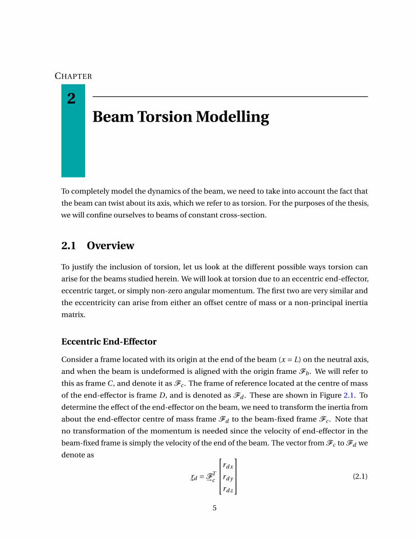
Consider a frame located with its origin at the end of the beam (x = L) on the neutral axis,
and when the beam is undeformed is aligned with the origin frame Fb . We will refer to
this as frame C , and denote it as Fc . The frame of reference located at the centre of mass
of the end-effector is frame D, and is denoted as Fd . These are shown in Figure 2.1. To
determine the effect of the end-effector on the beam, we need to transform the inertia from
about the end-effector centre of mass frame Fd to the beam-fixed frame Fc . Note that
no transformation of the momentum is needed since the velocity of end-effector in the
beam-fixed frame is simply the velocity of the end of the beam. The vector from Fc to Fd we
denote as
r~
d =F→Tc
rd x
rd y
rd z
(2.1)
5
Page 16
CHAPTER 2. BEAM TORSION MODELLING
bx
by
bz
Fb
cx
cy
cz
Fc dx
dy
dz
Fdrd→
Figure 2.1: End-Effector Reference Frames
where F→c is defined as,
F→c =
c~
x
c~
y
c~
z
(2.2)
The general parallel axis theorem [30] gives,
Ic = Id +me
(r 2
d y + r 2d z) −rd xrd y −rd xrd z
−rd xrd y (r 2d x + r 2
d z) −rd y rd z
−rd xrd z −rd y rd z (r 2d x + r 2
d y )
(2.3)
where me is the mass of the end-effector, Id is the inertia matrix about the centre of mass in
Fd . This assumes that Fc and Fd are not rotated with respect to each other. The case where
they are is effectively the same as the eccentric capture case dealt with below.
Now that the inertia is known, it is straightforward to calculate the angular momentum.
h~= Ic ω
~e (2.4)
where h~
is the angular momentum vector, and ω~
e is the angular velocity of the beam at x = L
(also the angular velocity of the end-effector),
ω~
e =F→Tc
θxL
ψyL
ψzL
(2.5)
where θxL is the rotation about the x-axis in the Fc frame, ψyL the rotation about the y-axis
in Fc , and ψzL the rotation about the z-axis in Fc . Therefore, the Fc x-coordinate angular
6
Page 17
2.1. OVERVIEW
bx
by
bz
Fb
cx
cy
cz
Fc dx
dy
dz
Fdrd→
ex
ey
ez
Fe
rce→
Figure 2.2: Post-Capture Target and End-Effector Reference Frames
momentum is,
hxL = (Id xx +me (r 2d y + r 2
d z))θxL − (Id x y + rd xrd y )ψyL − (Id xz + rd xrd z)ψzL (2.6)
The centre of mass of the end-effector will be some distance past the end of the beam, so
rd x 6= 0. If the centre of mass is not on the neutral axis at least one of rd y and rd z will be
non-zero. In that case, even if θxL = 0, there will be a non-zero torsional angular momentum.
Alternatively, if the inertia of the end-effector about its centre of mass is non-principal (ı.e.,
Id x y or Id xz 6= 0) the centre of mass could be on the neutral axis and still create non-zero
torsional angular momentum.
Eccentric Capture
In addition to the frames previously mentioned now we introduce an additional frame
E , denoted as Fe , located at the centre of mass of the target. Once captured, the target
contributes its mass and inertia to the system so the same effects as the end-effector can
be caused by the target in the post-capture case. This situation is shown in Figure 2.2.
Transforming the target velocities from the target frame Fe to the beam fixed frame F→c , we
use the vector from F→c to F→e ,
r~
ce =F→Tc
rex
re y
rez
(2.7)
7
Page 18
CHAPTER 2. BEAM TORSION MODELLING
As before, we have the general parallel axis theorem for the translation to F→b .
Ict = Ie +mt
(r 2
e y + r 2ez) −rexre y −rexrez
−rexre y (r 2ex + r 2
ez) −re y rez
−rexrez −re y rez (r 2ex + r 2
e y )
(2.8)
In general, the capture may have the two frames rotated with respect to one another. So, after
the translation we need to perform a rotational transformation on the matrix [30],
Ic = Rce Iet RTce (2.9)
where Rce is the rotation matrix needed to rotate F→e to F→c . This is dependent upon the
orientation at capture, so in general the target’s inertia matrix will be non-principal.
Since in the post-capture case, the target is part of the same rigid-body system as the
end-effector, we can consider that the target’s velocity at the end of the beam is the same as
the end-effector, we have the same situation as Equation (2.6), just with the inertia as given
in Equation (2.9). In this case, unless both the target and end-effector are specially designed,
the target’s centre of mass will be offset in at least one of the y or z directions. Therefore,
even without rotation of the frames, there will be some torsional angular momentum due to
the target’s capture.
2.2 Traditional Torsion Models
Pure torsion models of beams can be broken into two kinds, uniform torsion where the
beam in unrestrained,(where the same rate of twist occurs throughout the beam [31]) and
non-uniform torsion where an end is restrained.
Uniform Torsion
For uniform torsion, the two most prevalent models are those of St. Venant [31] and Timo-
shenko [32, 33]. Timoshenko’s model derives the equations of motion through differential
forces and moments acting on a section of the beam. This approach isn’t suitable for use with
variational principles. Since both the capture equations and finite element models herein
are derived using these, Timoshenko’s model isn’t useful for our purposes.
St. Venant’s model is based on assuming the form of the displacements. Consider the
cross-section shown in Figure 2.3. Let point P be located by a vector r~
P ,
r~
P =F→Ta
x
y
z
(2.10)
8
Page 19
2.2. TRADITIONAL TORSION MODELS
and is moved to point P ′ due to a rotation of the cross-section through an angle θ. The vector
to P ′, r~
P ′ is therefore,
r~
P ′ =F→Ta
x
y + v
z +w
(2.11)
The resulting displacement vector u~
is,
u~= r~
P ′ − r~
P =F→Ta
0
v
w
(2.12)
Assuming the angle of rotation is small, we can write the displacements as
v = −θz (2.13)
w = θy (2.14)
For a beam of constant cross-section, we have θ =αx, where α is the angle of twist per unit
length of the beam and x is the distance along the beam axis. We assume the displacements
due to warping (ı.e., axial displacements) are of the form u =αφ(y, z) where φ is a function
of y and z and is called the warping function. This leads to the following formulas for the
displacements of the beam.
u = αφ(y, z) (2.15)
v = −αxz (2.16)
w = αx y (2.17)
St. Venant further assumes that all the normal stresses are zero. This combined with the dis-
placement assumptions are used to derive the equations of motion/equilibrium. Complete
details are described in Appendix A.1.
Non-Uniform Torsion
While there is an extension to Timoshenko’s model for torsion that allows for non-uniform
torsion [32], for our purposes it suffers from the same difficulty that the uniform model
does. This also excludes the various coupled bending-torsion models that are based upon
Timoshenko’s torsion model [34, 35, 36, 37, 38, 39].
Reissner proposed models for non-uniform torsion [40] which are modifications to the
uniform torsion St. Venant model (see [31]) in that he assumes the in-plane deflections are
strictly due to rotation and he modifies how the warping is handled. In the first model, he
9
Page 20
CHAPTER 2. BEAM TORSION MODELLING
P (y, z)
P ′(y + v, z + w)
θv
w
y
z
Figure 2.3: Arbitrary Cross-Section
assumes a form for the axial deflection. In the second model, he instead assumes a form for
the axial stress. The axial stress form is mainly useful if one uses Reissner’s Variational Princi-
ple which uses a variation with respect to stresses and strains, but poses some difficulties if
one is to take variations with respect to other quantities.
Note that in both models, he assumes that the in-plane normal stresses (σy y and σzz)
on a cross-section are zero which implicitly assumes that Poisson effects are negligible. In
addition by assuming the in-plane deflections are strictly due to rotation the in-plane shear
τy z is zero.
The notation used herein is slightly different from the notation in Reissner’s paper mainly
because while Reissner oriented the z axis along the length of the beam, here we align the x
axis along the length.
While Reissner’s original models were static, the model that assumes a form for the axial
deflection was extended for dynamic problems by Barr [41] and later Ritchie and Leevers
[42, 43]. For this reason, along with the problems of the axial stress form, we will consider
the dynamic version of Reissner’s axial deflection form.
In the dynamic version of Reissner’s axial deflection form, we assume the deflection takes
the form,
u(x, y, z, t ) = φ(y, z)ψ(x, t ) (2.18)
v(x, y, z, t ) = −θ(x, t )z (2.19)
w(x, y, z, t ) = θ(x, t )y (2.20)
10
Page 21
2.2. TRADITIONAL TORSION MODELS
So, the main difference to St. Venant torsion is the replacement of the rate of twist with the
independent variable ψ(x, t ). If we follow Barr’s approach [41], we find that the equations of
motion are,
ρPψ = EPψ,xx −G(Kψ+Lcθ,x) (2.21)
ρ Jg θ = G(Jgθ,xx +Lcψ,x) (2.22)
where the constants are (see Appendix C for their calculation),
P =∫
Aφ(y, z)2dA (2.23)
K =∫
A
(φ,y (y, z)2 +φ,z(y, z)2)dA (2.24)
Lc =∫
A
(φ,z(y, z)y −φ,y (y, z)z
)dA (2.25)
Jg =∫
A(y2 + z2)dA (2.26)
where dA = dy dz, which is consistent with Ritchie and Leevers [42]. This is subject to the
boundary conditions on a constrained end,
ψ= θ = 0 (2.27)
and using Ritchie and Leevers condition on a free end (since it is a simpler but equivalent
form to Barr) in a consistent notation,
ψ,x = 0 (2.28)
T = G(Jgθ,x +Lcψ) = 0 (2.29)
where T is the transmitted torque at the free end. At this point, it’s possible to decouple the
equations, turning them into fourth order PDEs. However, both Barr and Ritchie and Leevers
oversimplify their solution for θ (and don’t solve for ψ) by assuming that the time modes are
cosine functions. Barr compounds the problem by assuming the spatial modes are cosine
functions as well; This assumption violates his boundary conditions at the constrained end.
Martinez and Ségura [44] use a static torsion model that is an extension of Reissner
torsion. In it they add an additional warping term to u so it becomes (keeping notation
consistent with the chapter),
u(x, y, z) =ψ(x)φ(y, z)+ηx(x, y, z) (2.30)
where ηx(x, y, z) is,
ηx(x, y, z) = f (x)g (y, z) (2.31)
This means we would need to solve for both warping functions φ and g .
11
Page 22
CHAPTER 2. BEAM TORSION MODELLING
Other Torsion Models
There are some simplified torsion models for use in coupled bending-torsion models [45,
46, 47, 48, 49, 50], but the models aren’t suitable for our particular problem because of their
modelling approach. The models [45, 47, 48, 50] start directly with a differential equation
which makes them unsuitable for use in a variational approach. Eslimy-Isfanany et al. [46]
uses a modal analysis approach which is also unsuitable for using in the variational equations.
Fischera et al. [49] also appear to use a modal analysis approach, but are vague on the specific
details of the system model. The coupled bending-torsion model by Klinkel and Govindjee
[51] is similar to traditional St. Venant/Reissner torsion models, but it assumes that the
warping doesn’t depend upon the axial coordinate. Given the boundary conditions, this
would not properly model non-uniform torsion.
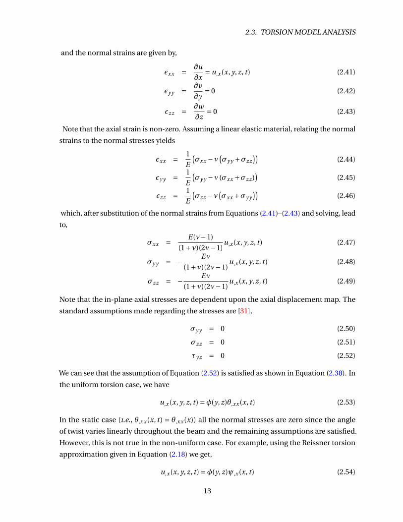
2.3 Torsion Model Analysis
In the traditional analysis of a beam in torsion (e.g., [31, 40]), the deflections are assumed to
be of the form
u = u(x, y, z, t ) (2.32)
v = −θ(x, t )z (2.33)
w = θ(x, t )y (2.34)
(see Figure 2.3) where it is assumed that θ(x, t ) is small. The shear strains, given in Equations
(2.32)–(2.34), are
γy z = ∂v
∂z+ ∂w
∂y= 0 (2.35)
γzx = ∂u
∂z+ ∂w
∂x= u,z(x, y, z, t )+ yθ,x(x, t ) (2.36)
γx y = ∂u
∂y+ ∂v
∂x= u,y (x, y, z, t )− zθ,x(x, t ) (2.37)
The corresponding shear stresses are,
τy z = Gγy z = 0 (2.38)
τzx = Gγzx =G(u,z(x, y, z, t )+ yθ,x(x, t )
)(2.39)
τx y = Gγx y =G(u,y (x, y, z, t )− zθ,x(x, t )
)(2.40)
12
Page 23
2.3. TORSION MODEL ANALYSIS
and the normal strains are given by,
εxx = ∂u
∂x= u,x(x, y, z, t ) (2.41)
εy y = ∂v
∂y= 0 (2.42)
εzz = ∂w
∂z= 0 (2.43)
Note that the axial strain is non-zero. Assuming a linear elastic material, relating the normal
strains to the normal stresses yields
εxx = 1
E
(σxx −ν
(σy y +σzz
))(2.44)
εy y = 1
E
(σy y −ν (σxx +σzz)
)(2.45)
εzz = 1
E
(σzz −ν
(σxx +σy y
))(2.46)
which, after substitution of the normal strains from Equations (2.41)–(2.43) and solving, lead
to,
σxx = E(ν−1)
(1+ν)(2ν−1)u,x(x, y, z, t ) (2.47)
σy y = − Eν
(1+ν)(2ν−1)u,x(x, y, z, t ) (2.48)
σzz = − Eν
(1+ν)(2ν−1)u,x(x, y, z, t ) (2.49)
Note that the in-plane axial stresses are dependent upon the axial displacement map. The
standard assumptions made regarding the stresses are [31],
σy y = 0 (2.50)
σzz = 0 (2.51)
τy z = 0 (2.52)
We can see that the assumption of Equation (2.52) is satisfied as shown in Equation (2.38). In
the uniform torsion case, we have
u,x(x, y, z, t ) =φ(y, z)θ,xx(x, t ) (2.53)
In the static case (ı.e., θ,xx(x, t) = θ,xx(x)) all the normal stresses are zero since the angle
of twist varies linearly throughout the beam and the remaining assumptions are satisfied.
However, this is not true in the non-uniform case. For example, using the Reissner torsion
approximation given in Equation (2.18) we get,
u,x(x, y, z, t ) =φ(y, z)ψ,x(x, t ) (2.54)
13
Page 24
CHAPTER 2. BEAM TORSION MODELLING
and ψ,x(x, t ) is not zero. So, the stress assumptions from Equations (2.50) and (2.51) and the
displacement assumptions as given in Equations (2.32)–(2.34) are inconsistent. For them to
be consistent, ψ(x, t ) would have to be linear in x.
It might be possible for the stress assumptions in Equations (2.50)– (2.52) to be satisfied
using Martinez and Ségura’s model, but that would impose the constraint,
ψ,x(x)φ(y, z) =− f,x(x)g (y, z) (2.55)
It would likely not be satisfied without explicit application of the constraint.
Since the first model isn’t consistent with the assumptions for non-uniform torsion
and the second requires the application of the constraint from Equation (2.55), we need to
consider other possibilities.
2.4 New Models for Torsion
Since we have two contradictory sets of assumptions in the non-uniform torsion case, we
will consider two possible models, each only using one set of assumptions.
Assumed Displacement Model
For simplicity we will restrict ourselves to beams of constant cross-section. Therefore, we
assume that each cross-section is warped in the same way and we will use Reissner’s axial
displacement map as given in (2.18). The torsional strain energy of a beam can be represented
as (assuming Equations (2.32)–(2.34)),
U = 1
2
∫V
(σxxεxx +τx yγx y +τzxγzx
)dV (2.56)
and after substitution of the stresses (Equations (2.39), (2.40), and (2.47)) and strains (Equa-
tions (2.36), (2.37), and (2.41)), along with the definition of u,x as given in Equation (2.54),
U = 1
2
∫V
E(ν−1)
(1+ν)(2ν−1)φ(y, z)2ψ,x(x, t )2 +G
(φ,y (y, z)ψ(x, t )− z θ,x(x, t )
)2
+G(φ,z(y, z)ψ(x, t )+ y θ,x(x, t )
)2 dV(2.57)
which we can simplify by introducing the constants P,K , and L, from Barr’s analysis (Equa-
tions (2.23)–(2.24)) and the constant,
η = (ν−1)
(1+ν)(2ν−1)(2.58)
14
Page 25
2.4. NEW MODELS FOR TORSION
This results in
U = 1
2
∫ L
0EηPψ,x(x, t )2 +G
(Kψ(x, t )2 + 2Lcθ,x(x, t )ψ(x, t )+ Jgθ,x(x, t )2)dx (2.59)
The torsional kinetic energy is,
Txt = 1
2
∫Vρ
(u2 + v2 + w 2)dV (2.60)
and after substitution of the assumed displacements we get,
Txt = 1
2
∫Vρ
(φ(y, z)2ψ(x, t )2 + (z2 + y2)θ(x, t )2)dV (2.61)
Then using the constants defined above this becomes
Txt = 1
2
∫ L
0ρ
(Pψ(x, t )2 + Jg θ(x, t )2)dx (2.62)
Hamilton’s action integral A is [52],
A =∫ t2
t1
L dt =∫ t2
t1
T −U dt (2.63)
where T is defined in Equation (2.62) (as Txt ) and U is defined in Equation (2.59) so the
action integral becomes,
A = 1
2
∫ t2
t1
∫ L
0
[ρ
(Pψ(x, t )2 + Jg θ(x, t )2)−EηPψ,x(x, t )2
− G(Kψ(x, t )2 +2Lcθ,x(x, t )ψ(x, t )+ Jgθ,x(x, t )2)]dxdt
(2.64)
Taking the variation of Equation (2.64) with respect to θ(x, t ) gives,
δA1 =∫ t2
t1
∫ L
0
[ρ Jg θ(x, t )δθ−G
(Lcψ(x, t ) + Jgθ,x(x, t )
)δθ,x
]dxdt = 0 (2.65)
Subsequent integration of Equation (2.65) by parts gives,
∫ L
0ρ Jg θ(x, t )δθdx
∣∣∣∣t2
t1−
∫ t2
t1G
(Lcψ(x, t )+ Jgθ,x(x, t )
)δθdt
∣∣∣∣L
0
−∫ t2
t1
∫ L
0
[ρ Jg θ(x, t )−G
(Lcψ,x(x, t )+ Jgθ,xx(x, t )
)]δθdxdt = 0
(2.66)
The variation of Equation (2.64) with respect to ψ(x, t ) gives
δA2 =∫ t2
t1
∫ L
0
[ρPψ(x, t )δψ−EηPψ,x(x, t )δψ,x − G
(Kψ+Lcθ,x
)δψ
]dxdt = 0 (2.67)
15
Page 26
CHAPTER 2. BEAM TORSION MODELLING
and integration of this by parts yields∫ L
0ρPψ(x, t )δψdx
∣∣∣∣t2
t1−
∫ t2
t1EηPψ,x(x, t )δψdt
∣∣∣∣L
0
−∫ t2
t1
∫ L
0
[ρPψ(x, t )−EηPψ,xx(x, t ) +G
(Kψ+Lcθ,x
)]δψdxdt = 0
(2.68)
From Equation (2.66) and (2.68) the equations of motion are found to be,
ρ Jg θ(x, t )−G(Lcψ,x(x, t )+ Jgθ,xx(x, t )
) = 0 (2.69)
ρPψ(x, t )−EηPψ,xx(x, t )+G(Kψ+Lcθ,x
) = 0 (2.70)
subject to the following initial and boundary conditions,∫ L
0ρPψ(x, t )δψdx
∣∣∣∣t2
t1= 0 (2.71)∫ L
0ρ Jg θ(x, t )δθdx
∣∣∣∣t2
t1= 0 (2.72)∫ t2
t1G
(Lcψ(x, t )+ Jgθ,x(x, t )
)δθdt
∣∣∣∣L
0= 0 (2.73)∫ t2
t1EηPψ,x(x, t )δψdt
∣∣∣∣L
0= 0 (2.74)
Aside from the addition of η from Equation (2.58), these equations of motion (and boundary
conditions) are consistent with the Reissner model in Equations (2.21) and (2.22). If we set ν
to zero in η, the equations reduce to the dynamic Reissner equations.
Note that this model has the same problem as the Reissner model described in Appendix
A.2, in that we can’t consider that φ is independent. Therefore, we will use the St. Venant
warping function (as derived in Appendix A.1). For other cases, one could use a numerical
approximation to the St. Venant warping function [53] or use a different warping function
[54, 55, 56] that is simpler to calculate.
Assumed Stress Model
If instead of assuming the displacements, we use the stress assumptions given in Equations
(2.50) and (2.51) we can get a new model for torsion (see Appendix A.3 for details). The
governing equations for this model are,
ρu − (E −2Gν)u,xx −G(u,y y +u,zz) = 0 (2.75)
ρv −G
(v,xx + v,zz + (1− 1
ν)v,y y
)= 0 (2.76)
ρw −G
(w,xx +w,y y + (1− 1
ν)w,zz
)= 0 (2.77)
16
Page 27
2.4. NEW MODELS FOR TORSION
The boundary conditions arising from the variations are,∫ t2
t1
∫A
Eu,xδu dAdt
∣∣∣∣L
0= 0 (2.78)∫ t2
t1
∫S
G[(
v,x +u,y)
ny +(w,x +u,z
)nz
]δu dSdt = 0 (2.79)∫ t2
t1
∫S
G[(u,y + v,x)nx + (v,z +w,y )nz]δv dSdt = 0 (2.80)∫ t2
t1
∫S
G[(u,z +w,x)nx + (v,z +w,y )ny ]δw dSdt = 0 (2.81)
and the initial conditions are, ∫VρuδudV
∣∣∣∣t2
t1
= 0 (2.82)∫Vρv δvdV
∣∣∣∣t2
t1
= 0 (2.83)∫VρwδwdV
∣∣∣∣t2
t1
= 0 (2.84)
with the additional constraints due to Poisson effects of,
v,y (x, y, z, t ) = −νu,x(x, y, z, t ) (2.85)
w,z(x, y, z, t ) = −νu,x(x, y, z, t ) (2.86)
The governing equations themselves aren’t difficult to solve for the general solution. However,
finding the solutions that meet both the boundary conditions and the Poisson constraints,
make an analytical solution extremely difficult. This would make working with it difficult
and as such won’t be used in the rest of the thesis.
17
Page 28
CHAPTER
3System Work, Kinetic, and Potential
Energy
In this chapter we examine the kinetic and potential energy of the system for different
beam and target models. Starting with the work and kinetic energy of the motor (since it is
independent of the beam model), then the target models, followed by the beam models, and
lastly, the end-effector models.
For the target and end-effector, we consider a point mass model, a 2D rigid body model,
and a 3D rigid body model. For the beam, we consider 2D Euler-Bernoulli and Timoshenko
beam models, as well as a 3D Timoshenko beam model including torsion. The 2D models
are based upon the system shown in Figure 3.1.
a~
x
a~
y
b~
x
b~
y
θ
dmr~
x
O
me
mt
Figure 3.1: 2D System Model
18
Page 29
3.1. MOTOR WORK AND KINETIC ENERGY
3.1 Motor Work and Kinetic Energy
The kinetic energy of the motor is given by
Tm = 1
2Jm θ
2 (3.1)
where Jm is the rotary inertia of the motor. The work done by the motor due to the generated
moment is,
W =∫ b
aM(θ)dθ (3.2)
where M(θ) is the generated moment of the motor.
3.2 Target Energy
This is the pre-capture target model. In the post capture case, the target is treated the same
as the end-effector.
Point Mass Model
The kinetic energy of a particle is,
Tp = 1
2mv~· v~
(3.3)
and the inertial velocity of the target is given by
v~
t =F→Ta
xt
yt
0
(3.4)
Hence, the kinetic energy of the target is
Tt = 1
2mt
(x2
t + y2t
)(3.5)
where mt is the mass of the target.
2D Rigid Body Model
The translational kinetic energy is the same as the point mass model, so we only need to add
the rotational kinetic energy. The angular velocity is,
ω~
t (t ) =F→Ta
0
0
γ(t )
(3.6)
19
Page 30
CHAPTER 3. SYSTEM WORK, KINETIC, AND POTENTIAL ENERGY
For both this model and the 3D rigid body model, it is assumed that the rotation is about an
axis that passes through the centre of mass. The rotational kinetic energy of a general rigid
body is,
Tr ot = 1
2ω~
T J ω~
(3.7)
where J is the inertia matrix for the body. For the target in this case, we assume that J is prin-
cipal and only the (3,3) component (Jt ) contributes to the kinetic energy. After substitution
Jt and of ω~
t (t ) for ω~
in Equation (3.7), the rotational kinetic energy of the target is,
Ttr = 1
2Jt γ(t )2 (3.8)
Therefore, the kinetic energy a 2D rigid body target is,
Tt = 1
2
(mt
(x2
t + y2t
)+ Jt γ(t )2) (3.9)
3D Rigid Body Model
The translational kinetic energy has an additional component due to the additional of a
z-coordinate velocity, which results in,
Tt = 1
2mt
(x2
t + y2t + z2
t
)(3.10)
The angular velocity is,
ω~
t (t ) =F→Ta
α(t )
β(t )
γ(t )
(3.11)
The rotational kinetic energy of a rigid body is as stated in Equation (3.7). For the target in
this case, we use the general inertia matrix,
Jt =
Jt xx Jt x y Jt xz
Jt x y Jt y y Jt y z
Jt xz Jt y z Jt zz
(3.12)
Resulting in the rotational kinetic energy of the target as,
Ttr = 1
2
(α2 Jt xx + β2 Jt y y + γ2 Jt zz +2αβJt x y +2αγJt xz +2βγJt y z
)(3.13)
Therefore, the total kinetic energy of a 3D rigid body target is,
Tt =1
2
(mt
(x2
t + y2t + z2
t
)+ α2 Jt xx + β2 Jt y y + γ2 Jt zz
+2αβJt x y +2αγJt xz +2βγJt y z) (3.14)
20
Page 31
3.3. BEAM ENERGY
3.3 Beam Energy
2D Euler-Bernoulli Beam
The position of a small differential element of the beam (see Figure 3.1) with a volume of
Adx is given by
r~
x =F→Tb
x − y v ′
y + v
0
(3.15)
where v = v(x, t ) is the transverse deflection of the beam neutral axis and v ′ is the slope of
that deflection. In this model, we are neglecting the axial extension of the beam. Transform-
ing to the inertial frame
r~
x =F→Ta Cab
x − y v ′
y + v
z
(3.16)
where Cab is,
Cab =
cosθ −sinθ 0
sinθ cosθ 0
0 0 1
(3.17)
Therefore, the position vector in the inertial frame is,
r~
x =F→Ta
(x − y v ′)cosθ− (y + v)sinθ
+(x − y v ′)sinθ+ (y + v)cosθ
z
(3.18)
Differentiating equation (3.18) with respect to time, we get the velocity of a differential
element of the beam.
v~
x =F→Ta
−(
v + θ(x − y v ′))
sinθ−(θ(y + v)+ y v ′)cosθ(
v + θ(x − y v ′))
cosθ−(θ(y + v)+ y v ′)sinθ
0
(3.19)
The kinetic energy of a flexible beam is given by
Tb = 1
2
∫Vρv~· v~
dV (3.20)
where ρ is the volume mass density. This can be reduced to
Tb = 1
2
∫ L
0ρAv~· v~
dx (3.21)
21
Page 32
CHAPTER 3. SYSTEM WORK, KINETIC, AND POTENTIAL ENERGY
substituting the differential beam element velocity derived in equation (3.19) we get the
following expression for the kinetic energy of the beam.
Tb = 1
2
∫ L
0ρA(x2θ2 +2xθv + v
2 + θ2v2)dx + 1
2
∫ L
0ρIy y (v ′2 +2v ′θ+ θ2(1+ v ′2))dx (3.22)
Since this is an Euler-Bernoulli beam, we will drop the v ′ terms (which arise from rotary
inertia), resulting in,
Tb = 1
2
∫ L
0ρA(x2θ2 +2xθv + v
2 + θ2v2)dx + 1
2
∫ L
0ρIy y θ
2dx (3.23)
The strain energy of the beam is given by
U = 1
2
∫ L
0E Iy y (v ′′)2dx (3.24)
where v ′′ is the second derivative of v with respect to x.
2D Timoshenko Beam
The position of a differential element of the rotating beam is given by,
r~
x =F→Tb
x +u − yψz
y + v
z
(3.25)
where u = u(x, t ), ψz =ψz(x, t ), and v = v(x, t ). In this formation, the axial extension of the
neutral axis is included via u(x, t ). Transforming to the inertial frame
r~
x =F→Ta Cab
x +u − yψz
y + v
z
(3.26)
where Cab is as given in Equation (3.17). The position of the differential element in the
inertial frame is therefore,
r~
x =F→Ta
(x +u − yψz)cosθ− (y + v)sinθ
(x +u − yψz)sinθ+ (y + v)cosθ
z
(3.27)
where θ = θ(t). Differentiating this with respect to time, we get the inertial velocity for a
differential element of the beam,
v~
x =F→Ta
[u − yψz − θ(y + v)]cosθ− [v + θ(x +u − yψz)]sinθ
[v + θ(x +u − yψz)]cosθ+ [u − θ(y + v)− yψz]sinθ
0
(3.28)
22
Page 33
3.3. BEAM ENERGY
substituting this into Equation (3.20) and integrating over the cross-section, we get the kinetic
energy of the beam,
Tb = 1
2
∫ L
0ρA
((v + θ(x +u))2 + (u − θv)2)dx + 1
2
∫ L
0ρIy y
((θ+ ψz)2 + θ2ψ2
z
)dx (3.29)
The strain energy of the beam is,
U = 1
2
∫ L
0(E Iy yψ
′2z +κ2G A(v ′−ψz)2 +E Au′2)dx (3.30)
3D Timoshenko Beam (with Torsion)
The position of a differential beam element in the rotating frame is given by,
r~
x =F→Tb
x +u(x, t )− yupv (x, t )− zupw (x, t )+Φ(x, y, z, t )
y + v(x, t )+V (x, y, z, t )
z +w(x, t )+W (x, y, z, t )
(3.31)
where u, v , and w are the deflections of the neutral axis, upv is the slope of the in-plane
bending curve, upw is the slope of the out of plane bending curve, and the functionsΦ, V ,
and W are general torsion functions. For Timoshenko beams, this becomes,
r~
x =F→Tb
x +u(x, t )− yψz(x, t )− zψy (x, t )+Φ(x, y, z, t )
y + v(x, t )+V (x, y, z, t )
z +w(x, t )+W (x, y, z, t )
(3.32)
Using the assumed displacement model from the last chapter, the torsion functions become,
Φ(x, y, z, t ) = φ(y, z)ψx(x, t ) (3.33)
V (x, y, z, t ) = −zθx(, t ) (3.34)
W (x, y, z, t ) = yθx(x, t ) (3.35)
where θx is the torsion angle (about the x-axis) and ψx is used to prevent confusion with the
bending angles. This results in the differential beam element position as,
r~
x =F→Tb
x +u(x, t )− yψz(x, t )− zψy (x, t )+φ(y, z)ψx(x, t )
y + v(x, t )− zθx(x, t )
z +w(x, t )+ yθx(x, t )
(3.36)
In order to get the kinetic and strain energy of the beam, we will split the deflection into two
contributions (in addition to the original position),
r~
x =F→Tb (r+db +dt ) (3.37)
23
Page 34
CHAPTER 3. SYSTEM WORK, KINETIC, AND POTENTIAL ENERGY
where r (the original position of the differential beam element) is,
r =
x
y
z
(3.38)
and db (the deflection due to extension and bending) is,
db =
u(x, t )− yψz(x, t )− zψy (x, t )
v(x, t )
w(x, t )
(3.39)
and dt (the deflection due to torsion) is,
dt =
φ(y, z)ψx(x, t )
−zθx(x, t )
yθx(x, t )
(3.40)
This split is done since we want Timoshenko’s shear correction factor applied only to the
shear contributions due to extension and bending. So, the inertial position for the extension
and bending contribution is,
r~
xb =F→Ta Cab
x +u(x, t )− yψz(x, t )− zψy (x, t )
y + v(x, t )
z +w(x, t )
(3.41)
and the torsion contribution is,
r~
xt =F→Ta Cab
φ(y, z)ψx(x, t )
−θx(x, t )z
θx(x, t )y
(3.42)
which upon expansion the former becomes,
r~
xb =F→Ta
(x +u − yψz + zψy )cosθ− (y + v)sinθ
(x +u + yψz + zψy )sinθ+ (y + v)cosθ
z +w
(3.43)
and the latter becomes,
r~
xt =F→Ta
φψx cosθ+ zθx sinθ
φψx sinθ− zθx cosθ
yθx
(3.44)
24
Page 35
3.3. BEAM ENERGY
Differentiating with respect to time for the bending and extension contributions,
v~
xb =F→Ta
(u − θ(y + v)− yψz − zψy
)cosθ− (
θ(x +u − zψy − yψz)+ v)
sinθ(θ(x +u − zψy − yψz)+ v
)cosθ+ (
u − θ(y + v)− yψz − zψy)
sinθ
w
(3.45)
and for the torsion contribution,
v~
xt =F→Ta
(φψx + θzθx
)cosθ− (
θφψx − zθx)
sinθ(θzθx +φψx
)sinθ+ (
θφψx − zθx)
cosθ
y θx
(3.46)
which after substituting into the beam energy equation given in Equation (3.20) and integrat-
ing over the cross-section yields,
Txb = 1
2
∫ L
0ρA
((v + θ(x +u))2 + (u − θv)2 + w
2)
dx
+ 1
2
∫ L
0ρ
(Iy y
((ψz + θ)2 + θ2ψ2
z
)+ Izz(ψ2y + θ2ψ2
y ))
dx
(3.47)
and the kinetic energy due to torsion is,
Txt = 1
2
∫ L
0ρ
(θ2(Pψ2
x + Izzθ2x)+ Jg θ
2x +Pψ2
x
)dx (3.48)
Note that P is the integral as given in Equation (2.23). The total kinetic energy of the beam is
the sum of these two,
Tb = Txb +Txt (3.49)
For the strain energy of the beam due to torsion, we will use Equation (2.59), but with the
additional assumption that ν≈ 0 to stay consistent with the Timoshenko beam assumptions.
This results in,
Uxt = 1
2
∫ L
0EPψ,x(x, t )2 +G
(Kψ(x, t )2 + 2Lcθ,x(x, t )ψ(x, t )+ Jgθ,x(x, t )2)dx (3.50)
See Appendix C for the calculation of P , K , and Lc . For the bending and extension contribu-
tion to strain energy, we have the following strains,
εxx = ∂u
∂x= ∂u
∂x− y
∂ψz
∂x− z
∂ψy
∂x(3.51)
γx y = ∂u
∂y+ ∂v
∂x= ∂v
∂x− ∂ψz
∂x(3.52)
γxz = ∂u
∂z+ ∂w
∂x= ∂w
∂x− ∂ψy
∂x(3.53)
25
Page 36
CHAPTER 3. SYSTEM WORK, KINETIC, AND POTENTIAL ENERGY
The corresponding stresses are,
σxx = Eεxx (3.54)
τx y = κ2Gγx y (3.55)
τxz = κ2Gγxz (3.56)
where κ2 is the shear correction factor. The strain energy is,
Uxb = 1
2
∫Vσxxεxx +τx yγx y +τxzγxzdV (3.57)
= 1
2
∫V
Eε2xx +κ2Gγ2
x y +κ2GγxzdV (3.58)
Using the strain expressions, after integration over the cross-section, this becomes,
Uxb = 1
2
∫ L
0
(E Au2
,x +E Iy yψ2z,x +E Izzψ
2y,x
+κ2G A(v ,x −ψz)2 +κ2G A(w ,x −ψy )2)dx
(3.59)
3.4 End-Effector Energy
a~
x
a~
y
b~
x
b~
y c~
xc~
y
θ
O
me
mt
de1
Figure 3.2: 2D System Model (with end-effector offset)
26
Page 37
3.4. END-EFFECTOR ENERGY
Point Mass (Euler-Bernoulli Beam)
The position of the end effector in the rotating frame (see Figure 3.2) is given by
r~
e =F→Tb
L
vL
0
+F→Tc
de1
0
0
(3.60)
where de1 is the offset of the point mass from the end of the beam. This assumes that the
centre of mass (CoM) of the end-effector is located along the neutral axis of the beam. This is
specified in a frame C fixed to the end of the beam. Note that in this particular case, we are
assuming no extension of the beam. Transforming to the inertial frame,
r~
e =F→Ta Cab
L
vL
0
+Cbc
de1
0
0
(3.61)
where Cbc is the rotation matrix from frame C to frame B. Cab is as before in Equation (3.17).
Restated again,
Cab =
cosθ −sinθ 0
sinθ cosθ 0
0 0 1
(3.62)
and Cbc is the matrix due to infinitesimal rotation as given in Meirovitch [57] (p. 107),
Cbc =
1 −∆θ3 ∆θ2
∆θ3 1 −∆θ1
−∆θ2 ∆θ1 1
(3.63)
where∆θi is the rotation of the frame C about axis i . In this case, only∆θ3 is non-zero giving,
Cbc =
1 −v ′
L 0
v ′L 1 0
0 0 1
(3.64)
Therefore, the position vector of the end effector centre of mass in the inertial frame is
r~
e =F→Ta
(L+de1)cosθ− (vL + v ′
Lde1)sinθ
(L+de1)sinθ+ (vL + v ′Lde1)cosθ
0
(3.65)
Differentiating this result with respect to time, we get the velocity of the end effector centre
of mass,
v~
e =F→Ta
−θ(vL + v ′
Lde1)cosθ−(vL +de1v ′
L + θ(L+de1))
sinθ(vL +de1v ′
L + θ(L+de1))
cosθ− θ(vL + v ′Lde1)sinθ
0
(3.66)
27
Page 38
CHAPTER 3. SYSTEM WORK, KINETIC, AND POTENTIAL ENERGY
Using this result in the equation for particle kinetic energy, Equation (3.3), we get,
Te = 1
2me
((vL + v ′
Lde1)+ (L+de1)θ)2 + 1
2me (vL + v ′
Lde1)2θ2 (3.67)
2D Rigid Body Model (Timoshenko Beam)
First, we define the position centre of mass of the end-effector in the beam frames as.
r~
e =F→Tb
L+uL
vL
0
+F→Tc
de1
0
0
(3.68)
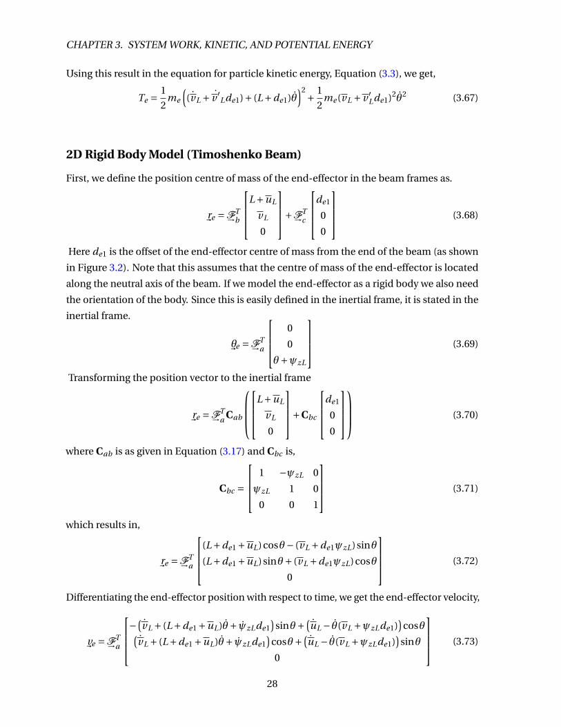
Here de1 is the offset of the end-effector centre of mass from the end of the beam (as shown
in Figure 3.2). Note that this assumes that the centre of mass of the end-effector is located
along the neutral axis of the beam. If we model the end-effector as a rigid body we also need
the orientation of the body. Since this is easily defined in the inertial frame, it is stated in the
inertial frame.
θ~
e =F→Ta
0
0
θ+ψzL
(3.69)
Transforming the position vector to the inertial frame
r~
e =F→Ta Cab
L+uL
vL
0
+Cbc
de1
0
0
(3.70)
where Cab is as given in Equation (3.17) and Cbc is,
Cbc =
1 −ψzL 0
ψzL 1 0
0 0 1
(3.71)
which results in,
r~
e =F→Ta
(L+de1 +uL)cosθ− (vL +de1ψzL)sinθ
(L+de1 +uL)sinθ+ (vL +de1ψzL)cosθ
0
(3.72)
Differentiating the end-effector position with respect to time, we get the end-effector velocity,
v~
e =F→Ta
−(
vL + (L+de1 +uL)θ+ ψzLde1)
sinθ+ (uL − θ(vL +ψzLde1)
)cosθ(
vL + (L+de1 +uL)θ+ ψzLde1)
cosθ+ (uL − θ(vL +ψzLde1)
)sinθ
0
(3.73)
28
Page 39
3.4. END-EFFECTOR ENERGY
and its corresponding angular velocity is,
ω~
e =F→Ta
0
0
θ+ ψzL
(3.74)
Substituting the velocity into Equation (3.3), we get the translational kinetic energy,
Tte = 1
2me
(vL + (uL +L+de1)θ+de1ψzL
)2 + 1
2me
(uL − (vL +de1ψzL)θ
)2(3.75)
The inertia matrix for the end-effector is assumed to be of the form,
Je =
J1 0 0
0 J2 0
0 0 Je
(3.76)
Using this and the angular velocity from Equation (3.74) in Equation (3.7),
Tr e = 1
2Je (θ+ ψzL)2 (3.77)
Therefore, the kinetic energy of the end-effector is of the form,
Te = 1
2me
(vL + (uL +L+de1)θ+de1ψzL
)2 + 1
2me
(uL − (vL +de1ψzL)θ
)2 + 1
2Je (θ+ ψzL)2
(3.78)
3D Rigid Body Model (Timoshenko Beam with Torsion)
bx
by
bz
Fb
cx
cy
cz
Fc dx
dy
dz
Fdd~
Figure 3.3: 3D end-effector offset
29
Page 40
CHAPTER 3. SYSTEM WORK, KINETIC, AND POTENTIAL ENERGY
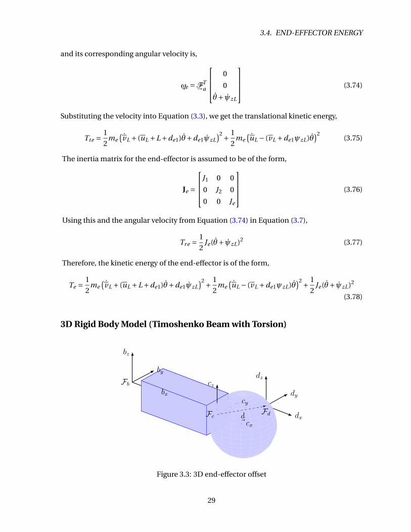
The frame of reference for the end-effector is located at the neutral axis of the beam
(see Figure 3.3). So, the position of the end-effector’s frame of reference can be found from
Equation (3.36) when x = L and both y and z are zero. This leads to,
r~
e =F→Tb
L+uL
vL
w L
+F→Tc
de1
de2
dd3
(3.79)
In this case, the end-effector has an offset of the vector d~
from the end of the beam. Note
that torsion has no direct contribution to the position since the reference frame is at the
neutral axis. However, it does affect the angular velocity of the end-effector. The position
vector in the inertial frame is,
r~
e =F→Ta Cab
L+uL
vL
w L
+Cbc
de1
de2
de3
(3.80)
where Cbc is,
Cbc =
1 −ψzL ψyL
ψzL 1 −θxL
−ψyL θxL 1
(3.81)
which results in,
r~
e =F→Ta
(L+uL +de1 −ψzLde2 +ψyLde3)cosθ− (vL +de2 +ψzLde1 −θxLde3)sinθ
(vL +de2 +ψzLde1 −θxLde3)cosθ+ (L+uL +de1 −ψzLde2 +ψyLde3)sinθ
w L +de3 −ψyLde1 +θxLde2
(3.82)
Differentiating with respect to time, we get the velocity of the end-effector in the inertial
frame,
v~
e = F→Ta
uL − θ(vL +de2 +ψzLde1 −θxLde3)+ ψyLde3 − ψzLde2
−(vL + ψzLde1 − θxLde3 + θ(L+uL +de1 −ψzLde2 +ψyLde3)
)0
cosθ
+ F→Ta
vL + ψzLde1 − θxLde3 + θ(L+uL +de1 −ψzLde2 +ψyLde3)
uL − θ(vL +de2 +ψzLde1 −θxLde3)+ ψyLde3 − ψzLde2
0
sinθ
+
0
0
w L − ψyLde1 + θxLde2
(3.83)
30
Page 41
3.4. END-EFFECTOR ENERGY
Which alternatively can be represented as,
v~
e =F→Ta
Kve1 cosθ−Kve2 sinθ
Kve2 cosθ+Kve1 sinθ
Kve3
(3.84)
where,
Kve1 = uL − θ(vL +de2 +ψzLde1 −θxLde3)+ ψyLde3 − ψzLde2 (3.85)
Kve2 = vL + ψzLde1 − θxLde3 + θ(L+uL +de1 −ψzLde2 +ψyLde3) (3.86)
Kve3 = w L − ψyLde1 + θxLde2 (3.87)
and the angular velocity is,
ω~
e =F→Ta
θxL
ψyL
θ+ ψzL
(3.88)
In general, the end-effector has an inertia matrix of the form,
Je =
Jexx Jex y Jexz
Jex y Je y y Je y z
Jexz Je y z Jezz
(3.89)
which we can transform from the body-centric reference frame to the end of the beam using
the formulas given in Chapter 2. Since the final product has the same form as given above,
we will use this form to determine the rotational kinetic energy from Equation (3.7) viz.,
Tr e = 1
2(Jexx θ
2xL + Je y yψ
2yL + Jezz(ψyL + θ)2)+ θxL(Jex yψyL + Jexz(θ+ψzL))+ Je y zψyL(θ+ψzL)
(3.90)
Similarly, the translational kinetic energy is,
Tte = 1
2me (K 2
ve1 +K 2ve2 +K 2
ve3) (3.91)
Now that the work, kinetic and strain energy is defined for each component in the system
(and for each model) we can use these results in subsequent chapters in the variational
principles to define the motion of the system (via Hamilton’s Principle) and the capture
equations (via Jourdain’s Variational Principle).
31
Page 42
CHAPTER
4Mixed Symbolic-Numeric Finite
Element Modelling
4.1 Introduction
In this chapter we are concerned with solving systems that can be derived through variational
principles (e.g., Hamilton’s Principle) [58]. Therefore, we have equations of the following
form to solve,
δ
∫ t1
t0
L(q,q′, t )dt = 0 (4.1)
where L (the Lagrangian) is a function of the column matrix q, the variable t and possibly
partial derivatives of q. The solution to this problem is a system of Euler-Lagrange equations
which take the form (assuming L(q,q′, t )),
∂
∂t
(∂L
∂qi
)− ∂
∂x
(∂L
∂q ′i
)− ∂L
∂qi= 0 (4.2)
The difficulty with these partial differential equations (PDEs) is that they often have no
known analytical solution. The standard approach to solving these PDEs is to use the Finite
Element Method (FEM) to approximate the solution. For common PDEs there are standard
finite element software packages that will solve these equations. However, for less common
problems we must derive the system of equations that result from using the finite element
method and then solve them (possibly with a standard package).
Symbolic techniques have been used in books [59, 60] to teach the finite element method
but their use has been limited calculation of the stiffness matrix for specific elements and
problems. Other work has been done on the derivation of optimized Fortran code using
Macsyma [61, 62, 63, 64] for evaluation of the element stiffness matrix.They symbolically
derive the strain-displacement relations and assume the stiffness matrix takes the form,
K =∫
VBT DB dV (4.3)
32
Page 43
4.2. OVERVIEW
where B is the strain-displacement matrix, D is the constitutive matrix, and the integral is
over the volume V . The work by Beltzer also assumes this form of the stiffness matrix. This
approach is fine if the forms of B and D for the specific problem are known but for more
complex problems these need to be derived.
More general work by Amberg [65] relates to the development of a software package,
“femLego”, built upon Maple and Fortran. Their software begins with the specification of the
weak form of the PDE and produces optimized Fortran code to solve the problem. However,
the weak form of the PDE can be difficult to derive. Also, their formulation handles time
domain solutions through finite differences and is limited in the types of elements and basis
functions that can be used. These requirements limit the types of problems that can be
solved.
Examining the previous work leads to the following goals for a new approach to the
problem,
1. All work deriving the system of equations can be done using the software;
2. that there is no inherent limitation to the types of elements and basis functions that
can be used;
3. static and dynamic problems are handled using the same approach.
4.2 Overview
The approach we are taking to derive and solve equations of the form given in Equation
(4.1) is to divide the problem into two stages. First, we derive the equations valid for a single
element in the finite element mesh using a symbolic computational approach. This is done
using a Symbolic Finite Element Method (SFEM) package in Maple that we have developed.
The second stage assembles the set of ODEs given these element matrices and a given mesh
then solves the resulting system numerically. While a number of programming languages
could be used for this task, Matlab is used because of its supporting facilities for numerical
computation and analysis. This two stage approach uses the strengths of both symbolic and
numeric computation.
An overview of the approach used to derive and solve the system equations is shown in
Figure 4.1. The first step, defining the Lagrangian, is problem specific and can typically be
handled using the standard Maple tools. The trial functions (ı.e., the approximations) used
in the SFEM package are of the form,
f (x, t ) =n∑
i=1φi (x)qi (t ) (4.4)
33
Page 44
CHAPTER 4. MIXED SYMBOLIC-NUMERIC FINITE ELEMENT MODELLING
LagrangianDefinition
Define theApproximations
Basis FunctionDefinition
MaterialsDefinition
ApproximatedLagrangian
Euler-LagrangeEquation
Problem-specificSimplification
Evaluation ofIntegrals
Formation ofElementMatrices
Definition ofElement Mesh
ODE SystemSolution
MatrixAssembly
SymbolicSteps
NumericalSteps
Figure 4.1: Element Matrix Calculation Process
34
Page 45
4.3. ASSEMBLY OF FULL MATRICES
whereφi (x) are the basis functions and qi (t ) are the nodal degrees-of-freedom (or nodal vari-
ables). Once the trial functions and Lagrangian are defined we substitute the trial functions
into the Lagrangian L and calculate the Euler-Lagrange equations:
d
dt
(∂L
∂qi
)= ∂L
∂qi+Qk (4.5)
where Qk are the generalized forces on the system. However, rather than calculating the
complete equation we instead calculate the individual terms and return them separately
since the left hand side leads to the mass matrix M while the right hand side leads to the
stiffness matrix K. Typically, after the Euler-Lagrange equation has been calculated there are
a number of simplifications that can be made.
The simplified results are combined with the definitions of the basis functions and the
materials (as they may vary spatially) to evaluate the integrals in the system. Lastly, the ele-
ment matrices are formed using the GenerateMatrix command from Maple’s LinearAlgebra
package.
Once the matrices are generated, we can use Maple’s code generation features to generate
optimized Matlab code which is output into separate functions for the mass and stiffness
element matrices to be used in the assembly process.
4.3 Assembly of Full Matrices
Application of Boundary Conditions
To apply a forced boundary condition, there are two main techniques:
1. Removal of the degrees of freedom from the system;
2. Modify the system of equations to enforce the constraint.
Since the first approach is more computationally efficient it is used. Since the system has
a pin joint at the hub, we will only consider the beam to be modelled as a cantilever beam
in a rotating frame. So our boundary conditions at x = 0 require us to remove the rows and
columns associate with the first node (for all element variables).
35
Page 46
CHAPTER 4. MIXED SYMBOLIC-NUMERIC FINITE ELEMENT MODELLING
Augmentation of Matrices with Rotational DOF
Note that the governing equations of the system can be written in matrix form as:
Mq+ Kq = F (4.6)
where,
M =[
0 0
0 M
]+
[J tT
t 0
]+Me (4.7)
K =[
0 0
0 K
](4.8)
F =
M(θ)
0
. . .
0
(4.9)
q =[θ
d
](4.10)
Therefore, the augmentation of the stiffness matrix can be performed by the addition of a
new row and column of all zeros. Augmentation of the mass matrix requires the calculation
of J (the effective inertia of the hub), t which is the contribution of the beam inertia to the
hub equation, and the matrix Me which is the contribution of the end-effector’s inertia to
the system. Note that the material mass and stiffness matrices M and K that are used in
these equations are the reduced DOF matrices resulting from the application of boundary
conditions.
4.4 Newmark-Beta Solver
Bathe and Wilson [66] present a version of the Newmark-Beta method that does not require
a prediction-correction step. The overview of the method as presented in Bathe and Wilson
[66] is presented below. Starting with the following equations,
Ut+∆t = Ut +((1−γ)Ut +γUt+∆t
)∆t (4.11)
Ut+∆t = Ut +Ut∆t + (( 1
2 −β)Ut +βUt+∆t)∆t (4.12)
where β and γ are parameters that are chosen for accuracy and stability. Setting β= 16 and
γ = 12 results in the linear acceleration method. Choosing β = 1
4 and γ = 12 results in an
unconditionally stable scheme [66, 67] which uses a constant average acceleration. Note that
36
Page 47
4.5. PURE TORSION CONVERGENCE TEST
Bathe and Wilson [66] recommend these settings for good accuracy and stability. We also
consider the equilibrium equations at time t +∆t ,
MUt+∆t +CUt+∆t +KUt+∆t = Ft+∆t (4.13)
In order to prevent the prediction-correction process, Bathe and Wilson [66] solve Equation
(4.11) for Ut+∆t in terms of Ut+∆t , and substitute the result into Equation (4.12). This results in
equations for Ut+∆t and Ut+∆t in terms of Ut+∆t alone. These equations are then substituted
into Equation (4.13) to solve for Ut+∆t . Then we can use the value of Ut+∆t to calculate Ut+∆t
and Ut+∆t .
According to Bathe and Wilson [66], to ensure unconditional stability for the damped
system, the following constraints on the parameters in Equations (4.11) and (4.12) hold:
γ≥ 12 (4.14)
β≥ 14 (γ+ 1
2 )2 (4.15)
In particular, we use the following values:
γ= 12 (4.16)
β= 14 (4.17)
This is also consistent with Heppler and Hansen [67] who state that
γ≥ 1
2β≥ 1
2γ (4.18)
is unconditionally stable for the damped system. Note that in the system of equations that
we are solving, none of our matrices depend upon time.
With this approach we can factorise the effective stiffness matrix once and only the
effective load vector needs to change at each timestep.
4.5 Pure Torsion Convergence Test
To test whether this system properly represents a dynamic system, we consider the case of a
fixed-free beam in pure torsion [68]. The natural frequency characteristic equation is [68],
ωn = (2n −1)πc
2L(4.19)
c =√
G
ρ(4.20)
If we normalize the modes of the finite element model with respect to these equations,
we get Figures 4.2 and 4.3. The first mode is nearly converged with just one element, but we
can see that we converge to the analytical solutions to the first eight modes in less than 10
elements, so the finite element model can accurately represent this pure torsion model.
37
Page 48
CHAPTER 4. MIXED SYMBOLIC-NUMERIC FINITE ELEMENT MODELLING
0 5 10 15 20 25 30 35 401
1.05
1.1
1.15
1.2
1.25
1.3
1.35
1.4
Number of Elements
Nor
mal
ized
Fre
quen
cy
Pure Torsion Finite Element Model − First Four Modes Convergence
First ModeSecond ModeThird ModeFourth Mode
Figure 4.2: Pure Torsion Modes 1 through 4 Convergence
38
Page 49
4.5. PURE TORSION CONVERGENCE TEST
0 5 10 15 20 25 30 35 401
1.05
1.1
1.15
1.2
1.25
1.3
1.35
1.4
1.45
Number of Elements
Nor
mal
ized
Fre
quen
cy
Pure Torsion Finite Element Model − Modes 5 through 8 Convergence
Fifth ModeSixth ModeSeventh ModeEighth Mode
Figure 4.3: Pure Torsion Modes 5 through 8 Convergence
39
Page 50
CHAPTER
5Modelling the Capture Dynamics
This chapter presents the theory used in the analysis of the mass capture. First, the equations
relating the pre- and post-impact velocities of a two particle system are presented. This is
done to justify the modelling of a plastic impact as a set of constraints. Second, an overview
of the variational theory of impact as presented in Bahar [29] is given. Next, we present a
three step process to model the dynamics of mass capture. Finally, the variational theory of
impact is applied to the system of interest.
5.1 Plastic Impact of Two Masses
Considering the impact of two smooth particles (Figure 5.1), the normal velocities before
and after impact are related by [69]:
v~
+2n − v
~
+1n =−e(v
~
−2n − v
~
−1n) (5.1)
where e is the coefficient of restitution. Given that these are particles, Brach [69] also states
that the tangential velocities are related by
v~
+1t = v
~
+2t (5.2)
Note that this is also true for rigid bodies with no sliding between the bodies. In the event of
plastic impact, the coefficient of restitution is zero, therefore, Equation (5.1) becomes
v~
+2n = v
~
+1n (5.3)
Therefore, for plastic impacts, we can model the impact as a constraint upon the velocities of
the particles. That is, after impact the velocities of the particles must be equal.
40
Page 51
5.2. VARIATIONAL METHODS FOR MASS CAPTURE
O
a2
a1
m2
V2t
V2n
m1
V1t
V1n
Figure 5.1: Two Particle Impact
5.2 Variational Methods for Mass Capture
From Bahar [29] the Jourdain Variational Principle (JVP) [28] is:
n∑i=1
[d
dt
(∂T
∂qi
)− ∂T
∂qi−Qi
]δqi = 0 (5.4)
where qi is the i -coordinate of the system, T is the kinetic energy of the system, and Qi is
applied impulsive force i . Note that this formulation requires that both δqi and δt be set
equal to zero. Integrating Equation (5.4) with respect to time [29] (see also Appendix E)
yields,n∑
i=1
[∆pi −Qi
]δqi = 0 (5.5)
where ∆pi is the increment in the generalised momentum:
∆pi = (pi )+− (pi )− (5.6)
between the pre-impact and post-impact states with Qi being the generalised impulse. The
generalised momentum pi of the state is given by [29]:
pi = ∂T
∂qi(5.7)
Therefore, Equation (5.5) can be written as
n∑i=1
[∂T
∂qi
+− ∂T
∂qi
−−Qi
]δqi = 0 (5.8)
41
Page 52
CHAPTER 5. MODELLING THE CAPTURE DYNAMICS
The above analysis holds for "true" velocities. However, Bahar [29] shows that the above also
holds when velocities are mapped to quasi-velocities1. This form is presented in Equation
(5.9) below.k∑
j=1
[∂T ∗
∂Q j
+− ∂T ∗
∂Q j
−− Π j
]δQ j = 0 (5.9)
where Q j are the quasi-velocities, ∂T ∗∂Q j
is the generalised quasi-momentum, and Π j is the
generalised quasi-impulse associated with the quasi-velocity Q j .
Note that any velocity constraint can be modelled as an additional quasi-velocity. A
plastic impact can be considered to be a set of velocity constraints as shown in Section 5.1.
Therefore, we can embed the constraints into the problem by converting to quasi-velocities.
This approach of constraint embedding differs from the approach done by Kövecses et al.
[3].
Since each of the quasi-velocity variations are independent, either the variation or the
term multiplying the variation must go to zero. The variations with respect to the constrained
quasi-velocities will be zero since the quasi-velocity values are fixed via the constraints after
impact and can be calculated before impact. Before, impact they will be defined by the initial
pre-impact conditions and after impact the quasi-velocities are set to satisfy the constraint.
However, the velocity variation with respect to the remaining quasi-velocities will not be
zero. Therefore, Equation (5.9) will result in a set of k −m (where m is the number of velocity
constraints) equations of the form,
∂T ∗
∂Q j
+− ∂T ∗
∂Q j
−− Π j = 0, j ∈ A (5.10)
where A is the set of unconstrained quasi-velocities. These equations relate the post-impact
velocities to the pre-impact velocities. It is important to note that this analysis assumes that
the capture process occurs instantaneously.
5.3 Analysis Process for Mass Capture Problems
The analysis process for mass capture problems is as follows:
1. Solve the pre-capture system of equations until time t1, the instant of impact/capture.
2. Use the final velocities from step 1 to determine post-capture velocities. This is done
using the variational method presented above.
1A quasi-velocity is a “linear combination of the generalized velocities, but they are not necessarily deriva-tives of any coordinates and thus cannot always be integrated to generalized coordinates.” [30] Examples ofquasi-velocities are Euler angles and nonholonmic constraints. Since the capture contraints are nonholonomicwe can model them as quasi-velocities.
42
Page 53
5.4. CAPTURE PROCESS MODELS
3. Solve the post-capture system of equations using the post-capture velocity results
from step 2 as initial conditions. Note that the position initial conditions are the same
as the final position of step 1, since the analysis in step 2 assumes that the impact is
instantaneous.
where the pre-capture and post-capture system of equations can be derived through tra-
ditional means (e.g., Hamilton’s Principle). This analysis process is consistent with the
approach taken by Kövecses et al. [27].
5.4 Capture Process Models
We will use the analysis process for different system models. The different models are:
1. A 2D Euler-Bernoulli beam (with no extension) and point masses for the target and the
end-effector;
2. A 2D Timoshenko beam (including extension) and 2D rigid bodies for the target and
the end-effector. It is assumed that the capture happens along the neutral axis of the
beam;
3. A 3D Timoshenko beam and 3D rigid bodies for the target and the end-effector. The
capture can happen anywhere.
Note that the 2D Euler-Bernoulli beam model included as a based of comparison with the
work done by Kövecses et al. [3, 4]. This chapter will show the complete process for the last
two cases and the results of the other first case. The details of the analysis for the first case
are shown in Appendix F.
5.5 2D Euler-Bernoulli Beam (with Point Masses) System
Considering a 2D Euler-Bernoulli beam (as in section 3.3 and point mass end-effector (section
3.4) and target (section 3.2), we get the following capture equations (complete details of the
43
Page 54
CHAPTER 5. MODELLING THE CAPTURE DYNAMICS
derivation are in Appendix F).
v+L =
me
(v−L + (L+de1)θ−+de1v ′−
L
)+mt
(y−
t cosθ0 − x−t sinθ0
)− (me +mt )(L+de1)θ+
2(mt +me )(5.11)
v ′+L = v
+L
de1(5.12)
v(x)+ = v(x)−−x(θ−− θ+) (5.13)
θ+ =(
Jm +me (v ′L0de1 + vL0)2 +∫ L
0 ρ(
Av0(x)2 + Iy y)
dx)θ−−mt (v ′
L0de1 + vL0)(x−t cosθ0 + y−
t sinθ0)
Jm + (me +mt )(v ′L0de1 + vL0)2 +∫ L
0 ρ(
Av0(x)2 + Iy y)
dx
(5.14)
Note that in contrast to the work of Kövecses et al. [3, 4], this 2D Euler-Bernoulli beam
model does not assume the end-effector is coincident with the end of the beam. Instead, we
allow for an offset so the point mass can be placed at the centre of mass of the end-effector.
Therefore, we have additional terms with v ′L0de1 and v ′
L. Also, our model includes beam
inertia (Iy y ) which is missing in theirs because their definition of an element of the beam is,
r~
xK =F→Tb
x
v
0
(5.15)
which is missing the y term in the second component as compared to Equation (3.15). The v ′
terms in Equation (3.15) are ignored in the kinetic energy of an Euler-Bernoulli beam so they
don’t affect the capture equations along the length. The only appear in the capture equations
at the end of the beam due to the offset of the end-effector.
5.6 2D Timoshenko Beam (with Rigid Bodies) System
Now we will consider a model in between the other two models set out in section 5.4. Here,
we have a 2D Timoshenko beam (as in section 3.3) and 2D rigid body end-effector (section
3.4) and target (section 3.2).
Post-capture velocity constraint
Since the capture is assumed to happen instantaneously, the position variables won’t change.
So, replacing the position variables (but not the velocities) with their values at the instant of
44
Page 55
5.6. 2D TIMOSHENKO BEAM (WITH RIGID BODIES) SYSTEM
capture (time t1),
v~
e = F→Ta
(uL − θ(vL0 +ψzL0de1)
)cosθ0 −
(vL + (L+de1 +uL0)θ+ ψzLde1
)sinθ0(
vL + (L+de1 +uL0)θ+ ψzLde1)
cosθ0 +(uL − θ(vL0 +ψzL0de1)
)sinθ0
0
(5.16)
ω~
e (t ) = F→Ta
0
0
θ(t )+ ψzL(t )
(5.17)
v~
t (t ) = F→Ta
xt (t )
yt (t )
0
(5.18)
ω~
t (t ) = F→Ta
0
0
γ(t )
(5.19)
v~
x = F→Ta
[u − yψz + θ(y + v0)]cosθ0 − [v − θ(x +u0 − yψz0)]sinθ0
[v − θ(x +u0 − yψz0)]cosθ0 + [u − yψz + θ(y + v0)]sinθ0
0
(5.20)
Modelling the capture process as a plastic collision, we get that the velocities before and
after impact must be equivalent. Since we are modelling the end-effector and target as rigid
bodies we equate both the translational and rotational velocities respectively. First, equating
the translational velocities yields,
xt (t ) = (uL − θ(vL0 +ψzL0de1)
)cosθ0 −
(vL + (L+de1 +uL0)θ+ ψzLde1
)sinθ0 (5.21)
yt (t ) = (vL + (L+de1 +uL0)θ+ ψzLde1
)cosθ0 +
(uL − θ(vL0 +ψzL0de1)
)sinθ0 (5.22)
and equating the rotational velocities gives,
γ(t ) = θ(t )+ ψzL(t ) (5.23)
Rearraging these equations so that all terms are on the left-hand side, leads to
xt (t )+ (vL + (L+de1 +uL0)θ+ ψzLde1
)sinθ0 −
(uL − θ(vL0 +ψzL0de1)
)cosθ0 = 0 (5.24)
yt (t )− (vL + (L+de1 +uL0)θ+ ψzLde1
)cosθ0 +
(uL − θ(vL0 +ψzL0de1)
)sinθ0 = 0 (5.25)
γ(t )− θ(t )− ψzL(t ) = 0 (5.26)
45
Page 56
CHAPTER 5. MODELLING THE CAPTURE DYNAMICS
Quasi-velocities
We now convert each of the beam and end-effector velocity variables to quasi-velocities.
Q1(t ) = ψz(x, t ) (5.27)
Q2(t ) = ψzL(t ) (5.28)
Q3(x, t ) = θ(t ) (5.29)
Q4(x, t ) = u(x, t ) (5.30)
Q5(x, t ) = uL(t ) (5.31)
Q6(t ) = v(x, t ) (5.32)
Q7(t ) = vL(t ) (5.33)
There are three remaining quasi-velocities necessary to completely define the system. The
three constraint equations (Equations (5.21) - (5.23)) are chosen to be the these three re-
maining quasi-velocities. So, substituting the quasi-velocity relations into the constraint
equations, yields
xt (t )+ (Q7 + (L+de1 +uL0)Q3 +Q2de1
)sinθ0 −
(Q5 −Q3(vL0 +ψzL0de1)
)cosθ0 = 0 (5.34)
yt (t )− (Q7 + (L+de1 +uL0)Q3 +Q2de1
)cosθ0 +
(Q5 −Q3(vL0 +ψzL0de1)
)sinθ0 = 0 (5.35)
γ(t )−Q3(t )−Q2(t ) = 0 (5.36)
Now we equate the left-hand side of each equation to a quasi-velocity variable according to,
Q8 = xt (t )+ (Q7 + (L+de1 +uL0)Q3 +Q2de1
)sinθ0 −
(Q5 −Q3(vL0 +ψzL0de1)
)cosθ0 (5.37)
Q9 = yt (t )− (Q7 + (L+de1 +uL0)Q3 +Q2de1
)cosθ0 +
(Q5 −Q3(vL0 +ψzL0de1)
)sinθ0 (5.38)
Q10 = γ−Q3 −Q2 (5.39)
Quasi-kinetic energy
To calculate the kinetic energy of the target it is necessary to rearrage the quasi-velocity
expressions in terms of the original target velocity variables (xt (t), yt (t), γ(t)). So, the new
translational velocity expression is,
v~
t (t ) =F→Ta
Q8 −
(Q7 + (L+de1 +uL0)Q3 +Q2de1
)sinθ0 +
(Q5 −Q3(vL0 +ψzL0de1)
)cosθ0
Q9 +(Q7 + (L+de1 +uL0)Q3 +Q2de1
)cosθ0 −
(Q5 −Q3(vL0 +ψzL0de1)
)sinθ0
0
(5.40)
and the new angular velocity is,
ω~
e (t ) =F→Ta
0
0
Q10(t )+Q3 +Q2
(5.41)
46
Page 57
5.6. 2D TIMOSHENKO BEAM (WITH RIGID BODIES) SYSTEM
The translational kinetic energy of a rigid body is,
Ttr ans = 1
2mv~· v~
(5.42)
For the target, this results in (for simplicity of form the variable dependence is left out),
T ∗t t = 1
2mt
((Q8 −Kt t1 sinθ0 +Kt t2 cosθ0
)2 + (Q9 +Kt t1 cosθ0 −Kt t2 sinθ0
)2)
(5.43)
where,
Kt t1 = Q7 + (L+de1 +uL0)Q3 +Q2de1 (5.44)
Kt t2 = Q5 −Q3(vL0 +ψzL0de1) (5.45)
Similarly, the rotational kinetic energy of a rigid body is,
Tr ot = 1
2ω~
J ω~
(5.46)
where J is the inertia matrix for the body. For the target in this case, the inertia matrix can be
stated as,
J =
Jt1 0 0
0 Jt2 0
0 0 Jt
(5.47)
Resulting in the rotational quasi-kinetic energy of the target as,
T ∗tr =
1
2Jt (Q10 +Q3 +Q2)2 (5.48)
The end-effector velocity using quasi-velocities is,
v~
e (t ) =F→Ta
((
Q5 −Q3(vL0 +ψzL0de1))
cosθ0 −Q7 + (L+de1 +uL0)Q3 +Q2de1)
sinθ0(Q7 + (L+de1 +uL0)Q3 +Q2de1
)cosθ0 +
(Q5 −Q3(vL0 +ψzL0de1)
)sinθ0
0
(5.49)
and its corresponding angular velocity is,
ω~
e (t ) =F→Ta
0
0
Q3(t )+Q2(t )
(5.50)
The inertia matrix for the end effector in this case is,
J =
Je1 0 0
0 Je2 0
0 0 Je
(5.51)
47
Page 58
CHAPTER 5. MODELLING THE CAPTURE DYNAMICS
This results in the following expressions for the translational and rotational quasi-kinetic
energies.
T ∗et =
1
2me
((Q7 + (L+de1 +uL0)Q3 +Q2de1
)2 + (Q5 −Q3(vL0 +ψzL0de1)
)2)
(5.52)
T ∗er =
1
2Je (Q3 +Q2)2 (5.53)
The quasi-kinetic energy due to the flexibility of the beam is in general,
Tb = 1
2
∫Vρ(v~
b · v~
b)dV (5.54)
where ρ is the volume mass density. In this case, v~
b is given by,
v~
b(x, t ) =F→Ta
[Q4 − yQ1 +Q3(y + v0)]cosθ0 − [Q6 −Q3(x +u0 − yψz0)]sinθ0
[Q6 −Q3(x +u0 − yψz0)]cosθ0 + [Q4 − yQ1 +Q3(y + v0)]sinθ0
0
(5.55)
Resulting in the following expression for the kinetic energy of the beam,
T ∗b = 1
2
∫Vρ
([Q4 − yQ1 +Q3(y + v0)]2 + [Q6 −Q3(x +u0 − yψz0)]
)dV (5.56)
The kinetic energy of the motor is,
T ∗m = 1
2JmQ2
3 (5.57)
where Jm is the inertia of the motor. The total quasi-kinetic energy of the system is given by
the sum of Equations (5.43), (5.48), (5.52), (5.53), (5.56), and (5.57).
48
Page 59
5.6. 2D TIMOSHENKO BEAM (WITH RIGID BODIES) SYSTEM
Generalised Quasi-momenta
The quasi-momenta for the system can be found by differentiating the total quasi-kinetic
energy of the system, as per
∂T ∗
∂Q1=
∫Vρ
(y2(Q1 +Q3)− y(Q4 − v0Q3)
)dV (5.58)
∂T ∗
∂Q2= (me +mt )de1
(de1(Q2 +Q3)+Q7 + (L+uL0)Q3
)+(Jt + Je )(Q2 +Q3)+mt de1(−Q8 sinθ0 +Q9 cosθ0)+ JtQ10 (5.59)
∂T ∗
∂Q3= ((Je + Jt )+ (me +mt )de1(L+uL0 +de1))Q2 + (Jm + Je + Jt )Q3
+(me +mt )((
(L+uL0 +de1)2 + (vL0 +de1ψzL0)2)Q3 + (L+uL0 +de1)Q7
+(vL0 +de1ψzL0)Q5)−mt
((vL0 +de1ψzL0)(Q8 cosθ0 +Q9 sinθ0) (5.60)
− (L+uL0 +de1)(−Q8 sinθ0 +Q9 cosθ0))+ JtQ10 +
∫Vρ
(−(y + v0)Q4
(x +u0 − yψz)Q6 + y(y + v0)Q1 +((x +u0 − yψz)2 + (y + v0)2)Q3
)dV
∂T ∗
∂Q4=
∫Vρ
(−v0Q3 +Q4 − y(Q3 +Q1))
dV (5.61)
∂T ∗
∂Q5= (me +mt )(Q5 −Q3(vL0 +de1ψzL0)+mt (Q8 cosθ0 +Q9 sinθ0) (5.62)
∂T ∗
∂Q6=
∫Vρ
(Q6 + (x +u0 − yψz0)Q3
)dV (5.63)
∂T ∗
∂Q7= (me +mt )(Q7 +Q3(L+uL0 +de1)+de1Q2)+mt (−Q8 sinθ0 +Q9 cosθ0)(5.64)
Note that we don’t need to calculate the quasi-momenta for the constraint quasi-variables
since the variation associated with these quasi-momenta is zero (as stated in section 5.2).
Velocity Relations
The results from the previous section are used in the Jourdain Variational Principle (JVP) [29],
10∑i=1
(∂T
∂Qi
+− ∂T
∂Qi
−)δQi = 0 (5.65)
where the superscript + indicates the post-capture quasi-momentum, superscript − indi-
cates the pre-capture quasi-momentum, and δQi is the variation with respect to quasi-
velocity i . The variation for i = 8,9,10 is zero since these quasi-velocities are constrained.
Therefore, we have velocity relations for i = 1..7 as stated in the following equations. First,
there is the velocity relation for the bending slope rate along the beam, ψz(x, t ),∫Vρy((y + v0)θ+− u(x)++ yψz(x)+)dV =
∫Vρy((y + v0)θ−− u(x)−+ yψz(x)−)dV (5.66)
49
Page 60
CHAPTER 5. MODELLING THE CAPTURE DYNAMICS
Next, the velocity relation for the bending slope of the end of the beam ψzL(t ),
(me +mt )de1
(v+L +de1ψ
+zL + (L+uL0 +de1)θ+
)+ (Je + Jt )(ψ+
zL + θ+) =(me +mt )de1
(v−L +de1ψ
−zL +L+uL0 +de1)θ−
)+ (Jt + Je )(ψ−zL + θ−)
+mt de1(−Q−8 sinθ0 +Q−
9 cosθ0)+ JtQ−10
(5.67)
The velocity relation for the angular velocity of the beam θ(t ).
(me +mt )((
(L+uL0 +de1)2 + (vL0 +de1ψzL0)2) θ+− (vL0 +de1ψzL0)u+L
+(L+uL0 +de1)(v+L +de1ψ
+zL)
)+ (Je + Jt )ψ+
zL + (Jm + Je + Jt )θ+
+∫ρ
(((x +u0 − yψz)2 + (y + v0)2) θ+− (y + v0)u
++ (x +u0 − yψz)v++ y(y + v0)ψ+
z
)dV
= (me +mt )((L+uL0 +de1)2 + (vL0 +de1ψzL0)2) θ−+ (Je + Jt )(ψ−
zL + θ−)+ Jm θ−
− (me +mt )(vL0 +de1ψzL0)u−L + (me +mt )de1(L+uL0 +de1)ψ−
zL + (me +mt )(L+uL0 +de1)v−L
+∫ρ(((x +u0 − yψz)2 + (y + v0)2)θ−− (y + v0)u
−+ (x +u0 − yψz)v−+ y(y + v0)ψ−
z )dV
−mt (vL0 +ψzL0de1)(Q−8 cosθ0 +Q−
9 sinθ0)+mt (L+uL0 +de1)(Q−9 cosθ0 −Q−
8 sinθ0)+ JtQ−10
(5.68)
The velocity relation for the extension of the beam u(x, t ),∫Vρ
(u(x)+− yψ+− (y + v0)θ+
)dV =
∫Vρ
(u(x)−− yψ−− (y + v0)θ−
)dV (5.69)
The velocity relation for the extension of the end of the beam uL(t ),
(me +mt )(u+L − (vL0 +ψzL0de1)θ+
)=(me +mt )
(uL − (vL0 +de1ψzL0)θ−
)+mt (Q−8 cosθ0
+Q−9 sinθ0)
(5.70)
The velocity relation for the transverse deflection of the beam v(x, t ),∫ρ((x +u0 − yψz0)θ++ v
+)dV =
∫ρ((x +u0 − yψz0)θ−+ v(x)−)dV (5.71)
and finally, the velocity relation for the transverse deflection of the end of the beam vL(t ),
(me +mt )(v+L +de1ψ
+zL + (L+uL0 +de1)θ+) =(me +mt )(v
−L +de1ψ
−zL + (L+uL0 +de1)θ−)
+mt (−Q−8 sinθ0 +Q−
9 cosθ0)
(5.72)
50
Page 61
5.6. 2D TIMOSHENKO BEAM (WITH RIGID BODIES) SYSTEM
Now, we substitute the constraint equations in for Q8, Q9 and Q10 into Equations (5.66)–
(5.72). The bending slope along the beam is unchanged,∫Vρy((y + v0)θ+− u(x)++ yψz(x)+)dV =
∫Vρy((y + v0)θ−− u(x)−+ yψz(x)−)dV (5.73)
and the bending slope at the end of the beam becomes,
(me +mt )de1
(v+L + (L+uL0 +de1)θ++de1ψ
+zL
)+ (Je + Jt )(ψ+
zL + θ+)
= me de1(v−L +de1ψ
−zL + (L+uL0 +de1)θ−
)+ Je (ψ−zL + θ−)+mt de1(y−
t cosθ0 − x−t sinθ0)+ Jt γ
−
(5.74)
The velocity relation for the angular velocity of the beam becomes,
(me +mt )((
(L+uL0 +de1)2 + (vL0 +de1ψzL0)2) θ++ (vL0 +de1ψzL0)u+L
−(L+uL0 +de1)(v+L +de1ψ
+zL)
)+ (Je + Jt )ψ+
zL + (Jm + Je + Jt )θ+
+∫ρ
(((x +u0 − yψz)2 + (y + v0)2) θ++ (y + v0)u
+− (x +u0 − yψz)v+− y(y + v0)ψ+
z
)dV
= me((L+uL0 +de1)2 + (vL0 +de1ψzL0)2) θ−+ Je (ψ−
zL + θ−)+ Jm θ−
+me (vL0 +de1ψzL0)u−L −me (L+uL0 +de1)v
−L −me de1(L+uL0 +de1)ψ−
zL
+∫ρ(((x +u0 − yψz)2 + (y + v0)2)θ−+ (y + v0)u
−− (x +u0 − yψz)v−− y(y + v0)ψ−
z )dV
+mt (vL0 +de1ψzL0)(x−t cosθ0 − y−
t sinθ0)−mt (L+uL0 +de1)(x−t sinθ0 + y−
t cosθ0)+ Jt γ−
(5.75)
The velocity relation for the extension of the beam is unchanged as,∫Vρ
(u(x)+− yψ+− (y + v0)θ+
)dV =
∫Vρ
(u(x)−− yψ−− (y + v0)θ−
)dV (5.76)
and the velocity relation for the extension of the end of the beam is,
(me +mt )(u+L − (vL0 +de1ψzL0)θ+
)= me
(u−L − (vL0 +de1ψzL0)θ−
)+mt (x−t cosθ0 + y−
t sinθ0)
(5.77)
The transverse deflection velocity relation is unchanged,∫ρ((x +u0 − yψz0)θ++ v
+)dV =
∫ρ((x +u0 − yψz0)θ−+ v(x)−)dV (5.78)
but the transverse deflection velocity relation for the end of the beam becomes,
(me +mt )(v+L +de1ψ
+zL + (L+uL0 +de1)θ+) =me (v
−L +de1ψ
−zL + (L+uL0 +de1)θ−)
+mt (y−t cosθ0 − x−
t sinθ0)(5.79)
51
Page 62
CHAPTER 5. MODELLING THE CAPTURE DYNAMICS
Under the assumption that the x-axis corresponds to the centroidal axis of the beam we can
simplify the integrals using, ∫ ∫dydz = A(x) (5.80)∫ ∫ydydz = 0 (5.81)∫ ∫y2dydz = Iy y (x) (5.82)
which means the equations (5.73)–(5.79) become, respectively,∫ L
0ρIy y (x)
(ψ+
z + θ+)dx =
∫ L
0ρIy y (x)
(ψ−
z + θ−)dx (5.83)
(me +mt )de1
(v+L − (L+uL0 +de1)θ++de1ψ
+zL
)+ (Je + Jt )(ψ+
zL + θ+)
= me de1(v−L +de1ψ
−zL − (L+uL0 +de1)θ−
)+ Je (ψ−zL + θ−)+mt de1(x−
t sinθ0 + y−t cosθ0)+ Jt γ
−
(5.84)
(me +mt )((
(L+uL0 +de1)2 + (vL0 +de1ψzL0)2) θ++ (vL0 +de1ψzL0)u+L
+(L+uL0 +de1)(v+L +de1ψ
+zL)
)+ (Je + Jt )ψ+
zL + (Jm + Je + Jt )θ+
+∫ L
0ρ
(A
(((x +u0)2 + v2
0)θ+− v0u++ (x +u0)v
+)+ Iy y
((1+ψ2
z0)θ++ ψ+))dx
= me((L+uL0 +de1)2 + (vL0 +de1ψzL0)2) θ−+ Je (ψ−
zL + θ−)+ Jm θ−
+me (vL0 +de1ψzL0)u−L −me (L+uL0 +de1)v
−L +me de1(L+uL0 +de1)ψ−
zL
+∫ L
0ρ
(A
(((x +u0)2 + v2
0)θ−− v0u−+ (x +u0)v
−)+ Iy y((1+ψ2
z0)θ−+ ψ−))dx
−mt (vL0 +de1ψzL0)(x−t cosθ0 + y−
t sinθ0)+mt (L+uL0 +de1)(y−t cosθ0 − x−
t sinθ0)+ Jt γ−
(5.85)
∫ L
0ρA(x)
(u(x)+− v0(x)θ+
)dx =
∫ L
0ρA(x)
(u(x)−− v0(x)θ−
)dx (5.86)
(me +mt )(u+L − (vL0 +de1ψzL0)θ+
)= me
(u−L − (vL0 +de1ψzL0)θ−
)+mt (x−t cosθ0 − y−
t sinθ0)
(5.87)
∫ L
0ρA(x)
(v(x)++ (x +u0(x))θ+
)dx =
∫ L
0ρA(x)
(v(x)−+ (x +u0(x))θ−
)dx (5.88)
52
Page 63
5.6. 2D TIMOSHENKO BEAM (WITH RIGID BODIES) SYSTEM
(me +mt )(v+L +de1ψ
+zL + (L+uL0 +de1)θ+) =me (v
−L +de1ψ
−zL + (L+uL0 +de1)θ−)
+mt (y−t cosθ0 − x−
t sinθ0)(5.89)
Leaving aside Equation (5.85) for the moment, we will simplify the remaining equations.
Note that because the integrals are over the same domain and range, we will simply equate
the integrands where appropriate,
ψ(x)+ = ψ(x)−− θ++ θ− (5.90)
ψ+zL = me de1
(v−L +de1ψ
−zL − (L+uL0 +de1)θ−
)+ Je (ψ−zL + θ−)+ Jt γ
−
(me +mt )d 2e1 + (Je + Jt )
+mt de1(x−t sinθ0 + y−
t cosθ0)− (Je + Jt )θ+
(me +mt )d 2e1 + (Je + Jt )
−(me +mt )de1
(v+L + (L+uL0 +de1)θ+
)(me +mt )d 2
e1 + (Je + Jt )(5.91)
u(x)+ = u(x)−− v0(x)(θ+− θ−) (5.92)
u+L = me
(u−L − (vL0 +de1ψzL0)θ−
)+mt (x−t cosθ0 + y−
t sinθ0)
me +mt
+(vL0 +de1ψzL0)θ+ (5.93)
v(x)+ = v(x)−+ (x +u0(x))(θ−− θ+) (5.94)
v+L = me (v
−L +de1ψ
−zL + (L+uL0 +de1)θ−)+mt (y−
t cosθ0 − x−t sinθ0)
(me +mt )
−(de1ψ+zL + (L+uL0 +de1)θ+) (5.95)
After substituting these results into Equation (5.85) and simplifying, we find that
θ+ = θ− (5.96)
53
Page 64
CHAPTER 5. MODELLING THE CAPTURE DYNAMICS
which means the final set of equations (5.90)–(5.96) can be written as,
ψz(x)+ = ψz(x)− (5.97)
ψ+zL = Jt (γ−− θ−)+ Jeψ
−zL
Jt + Je(5.98)
u(x)+ = u(x)− (5.99)
u+L = mt
(x−
t cosθ+ y−t sinθ+ (vL +de1ψzL)θ−
)+me u−L
mt +me(5.100)
v(x)+ = v(x)− (5.101)
v+L = me v
−L +mt
(y−
t cosθ− x−t sinθ− θ−(uL +L+de1)
)mt +me
+de1 Jt (θ−− γ−)
Jt + Je+ de1ψ
−zL(me Jt −mt Je )
(mt +me )(Jt + Je )(5.102)
θ+ = θ− (5.103)
From these we can note that only the tip velocities (Equations (5.98), (5.100), and (5.102)) are
directly affected by the capture event. Also of importance is that the angular velocity changes
are taken strictly by the rotation of the end-effector, not the beam. So in this case, we see the
tip velocities updated and then the changes will propagate down the beam.
5.7 General Beam Capture
In this case, we are considering a 3D beam model (including torsion) and general rigid
bodies for both the end-effector and target. The capture can happen at any point on the end-
effector and target. Because of the torsion model, we do assume that the beam cross-section
is constant along the beam.
Post-Capture Velocity Constraint
Modelling the capture process as a plastic collision, from Section 5.1 we get that the velocities
at impact must be equivalent. Therefore, our velocity constraint is that after capture the target
velocity and end effector velocities have to match. Since both the target and end-effector are
rigid bodies, we assume that they contact at a minimum of one point post-capture and that
the target and end-effector have the same velocity at that point.
The target velocity given in Equation (3.4) is for the centre of mass, not the point of
contact. So, assuming a vector r~
tc from the centre of mass to the point of contact, we need to
54
Page 65
5.7. GENERAL BEAM CAPTURE
bx
by
bz
Fb
cx
cy
cz
Fc dx
dy
dz
Fd
ret→
ex
ey
ez
Fe
rtc→
Figure 5.2: 3D Target Capture
add the additional velocity (see Figure 5.2),
v~
tc (t ) = ω~
t × r~
tc (5.104)
= F→Ta
rtc3β
−rtc3α
rtc2α− rtc1β
(5.105)
Therefore, the translational velocity at the point of contact is,
v~
c (t ) =F→Ta
xt + rtc3β
yt − rtc3α
zt + rtc2α− rtc1β
(5.106)
The end-effector velocity is given in Equation (3.83), but we need the velocity at the point of
contact. The velocity at the point of contact has an additional component from the offset of
the contact point from the centre of mass, given by vector r~
et (see Figure 5.2),
v~
et (t ) = ω~
e × r~
et (5.107)
= F→Ta
−(θ+ ψzL)
((ret1 −ψzLret2 +ψyLret3)sinθ+ (−ψzLret1 − ret2 +θxLret3)cosθ
)(θ+ ψzL)
(−ψzLret1 − ret2 +θxLret3)sinθ+ (ret1 −ψzLret2 +ψyLret3)cosθ)
−ψyL((ret1 −ψzLret2 +ψyLret3)cosθ+ (ψzLret1 + ret2 −θxLret3)sinθ
)
+
−ψyL
(ψyLret1 −θxLret2 − ret3
)θxL
(ψyLret1 −θxLret2 − ret3
)θxL
((ψzLret1 + ret2 −θxLret3)cosθ+ (ret1 −ψzLret2 +ψyLret3)sinθ
) (5.108)
55
Page 66
CHAPTER 5. MODELLING THE CAPTURE DYNAMICS
which we can write as,
v~
et (t ) =
(θ+ ψzL)(−Ket1 sinθ+Ket2 cosθ)−Ket3ψyL
(θ+ ψzL)(Ket2 sinθ+Ket1 cosθ)+Ket3θxL
θxL(−Ket2 cosθ+Ket1 sinθ)− ψyL(Ket1 cosθ−Ket2 sinθ)
(5.109)
where Ket1, Ket2, and Ket3 are defined as,
Ket1 = ret1 −ψzLret2 +ψyLret3 (5.110)
Ket2 = −ψzLret1 − ret2 +θxLret3 (5.111)
Ket3 = ψyLret1 −θxLret2 − ret3 (5.112)
Note that during capture all of these are considered to be constant. The velocity at the point
of contact is defined by,
v~
ec = v~
e + v~
et (5.113)
where v~
e is as defined in Equation (3.84). Therefore, The velocity of the end-effector at the
contact point is,
v~
ec (t ) =F→Ta
(Kve1 +Ket2(θ+ ψzL)
)cosθ− (
Kve2 +Ket1(θ+ ψzL))
sinθ−Ket3ψyL(Kve2 +Ket1(θ+ ψzL)
)cosθ+ (
Kve1 +Ket2(θ+ ψzL))
sinθ+Ket3θxL
Kve3 + θxL(−Ket2 cosθ+Ket1 sinθ)− ψyL(Ket1 cosθ+Ket2 sinθ)
(5.114)
In this equation, Kve1, Kve2, and Kve3 contain velocities and as such are not constant during
capture which means we will need to redefine them in terms of quasi-velocities later. The
velocities of the target and the end-effector at the point of contact are given in the inertial
frame so we can subtract components to get the following constraints,
xt + rtc3β+Ket3ψyL −(Kve1 +Ket2(θ+ ψzL)
)cosθ
+(Kve2 +Ket1(θ+ ψzL)
)sinθ = 0 (5.115)
yt − rtc3α−Ket3θxL −(Kve2 +Ket1(θ+ ψzL)
)cosθ
−(Kve1 +Ket2(θ+ ψzL)
)sinθ = 0 (5.116)
zt + rtc2α+ rtc1β−Kve3 − θxL(−Ket2 cosθ+Ket1 sinθ)
+ψyL(Ket1 cosθ+Ket2 sinθ) = 0 (5.117)
Since we are considering the impact duration to be infinitesimal, all position variables
can be replaced with their value at impact (θ(t) = θ(t1), u(L, t) = u(L, t1), v(L, t) = v(L, t1),
56
Page 67
5.7. GENERAL BEAM CAPTURE
w(L, t ) = w(L, t1) ) which we will denote as θ0, uL0, vL0 and w L0 respectively.
xt + rtc3β+Ket3ψyL −(Kve1 +Ket2(θ+ ψzL)
)cosθ0
−(Kve2 +Ket1(θ+ ψzL)
)sinθ0 = 0 (5.118)
yt − rtc3α−Ket3θxL −(Kve2 +Ket1(θ+ ψzL)
)cosθ0
−(Kve1 +Ket2(θ+ ψzL)
)sinθ0 = 0 (5.119)
zt + rtc2α+ rtc1β−Kve3 − θxL(−Ket2 cosθ0 +Ket1 sinθ0)
+ψyL(Ket1 cosθ0 +Ket2 sinθ0) = 0 (5.120)
where Ket1, Ket2, Ket3, Kve1, Kve2, and Kve3 become,
Ket1 = ret1 −ψzL0ret2 +ψyL0ret3 (5.121)
Ket2 = −ψzL0ret1 − ret2 +θxL0ret3 (5.122)
Ket3 = ψyL0ret1 −θxLret2 − ret3 (5.123)
Kve1 = uL − θ(vL0 +de2 +ψzL0de1 −θxL0de3)+ ψyLde3 − ψzLde2 (5.124)
Kve2 = vL + ψzLde1 − θxLde3 + θ(L+uL0 +de1 −ψzL0de2 +ψyL0de3) (5.125)
Kve3 = w L − ψyLde1 + θxLde2 (5.126)
Similarly, for the angular velocities,
α(t )− θxL(t ) = 0 (5.127)
β(t )− ψyL(t ) = 0 (5.128)
γ(t )− θ(t )− ψzL(t ) = 0 (5.129)
57
Page 68
CHAPTER 5. MODELLING THE CAPTURE DYNAMICS
Quasi-Velocities
Representing each of the beam and end-effector velocity variables as quasi-velocities,
Q1(x, t ) = ψx(x, t ) (5.130)
Q2(x, t ) = ψy (x, t ) (5.131)
Q3(t ) = ψyL(t ) (5.132)
Q4(x, t ) = ψz(x, t ) (5.133)
Q5(t ) = ψzL(t ) (5.134)
Q6(t ) = θ(t ) (5.135)
Q7(x, t ) = θx(x, t ) (5.136)
Q8(x, t ) = u(x, t ) (5.137)
Q9(t ) = uL(t ) (5.138)
Q10(x, t ) = v(x, t ) (5.139)
Q11(t ) = vL(t ) (5.140)
Q12(x, t ) = w(x, t ) (5.141)
Q13(t ) = w L(t ) (5.142)
Q14(t ) = θxL(t ) (5.143)
There are six remaining quasi-velocities to completely define the system corresponding to
the translation and rotation constraints. Starting with the translation constraints,
Q15 = xt + rtc3β+Ket3Q3 −(Kve1 +Ket2(Q6 +Q5)
)cosθ0
−(Kve2 +Ket1(Q6 +Q5)
)sinθ0 (5.144)
Q16 = yt − rtc3α−Ket3Q14 −(Kve2 +Ket1(Q6 +Q5)
)cosθ0
−(Kve1 +Ket2(Q6 +Q5)
)sinθ0 (5.145)
Q17 = zt + rtc2α+ rtc1β−Kve3 −Q14(−Ket2 cosθ0 +Ket1 sinθ0)
+Q3(Ket1 cosθ0 +Ket2 sinθ0) (5.146)
where Kve1, Kve2, and Kve3 are now as follows,
Kve1 = Q9 −Q6(vL0 +de2 +ψzL0de1 −θxL0de3)+Q3de3 −Q5de2 (5.147)
Kve2 = Q11 +Q5de1 −Q14de3 +Q6(L+uL0 +de1 −ψzL0de2 +ψyL0de3) (5.148)
Kve3 = Q13 −Q3de1 +Q14de2 (5.149)
58
Page 69
5.7. GENERAL BEAM CAPTURE
and the rotation constraints,
Q18(t ) = α(t )− θxL(t ) (5.150)
Q19(t ) = β(t )− ψyL(t ) (5.151)
Q20(t ) = γ(t )− θ(t )− ψzL(t ) (5.152)
Substituting the quasi-velocities into the rotation constraints,
Q18(t ) = α(t )−Q14(t ) (5.153)
Q19(t ) = β(t )−Q3(t ) (5.154)
Q20(t ) = γ(t )−Q6(t )−Q5(t ) (5.155)
which can be re-arranged for the angular velocities gives,
α(t ) = Q18(t )+Q14(t ) (5.156)
β(t ) = Q19(t )+Q3(t ) (5.157)
γ(t ) = Q20(t )+Q6(t )+Q5(t ) (5.158)
Substituting these into Equations (5.144)–(5.146) we get the quasi-velocities for the transla-
tional constraints,
Q15 = xt + rtc3(Q19 +Q3)+Ket3Q3 −(Kve1 −Ket2(Q6 +Q5)
)cosθ0
−(Kve2 +Ket1(Q6 +Q5)
)sinθ0 (5.159)
Q16 = yt − rtc3(Q18 +Q14)−Ket3Q14 −(Kve2 +Ket1(Q6 +Q5)
)cosθ0
−(Kve1 −Ket2(Q6 +Q5)
)sinθ0 (5.160)
Q17 = zt + rtc2(Q18 +Q14)+ rtc1(Q19 +Q3)−Kve3 −Q14(−Ket2 cosθ0 −Ket1 sinθ0)
+Q3(Ket1 cosθ0 +Ket2 sinθ0) (5.161)
and re-arranging for the target velocities,
xt = Q15 − rtc3(Q19 +Q3)−Ket3Q3 +(Kve1 +Ket2(Q6 +Q5)
)cosθ0
+(Kve2 +Ket1(Q6 +Q5)
)sinθ0 (5.162)
yt = Q16 + rtc3(Q18 +Q14)+Ket3Q14 +(Kve2 +Ket1(Q6 +Q5)
)cosθ0
+(Kve1 −Ket2(Q6 +Q5)
)sinθ0 (5.163)
zt = Q17 − rtc2(Q18 +Q14)− rtc1(Q19 +Q3)+Kve3 +Q14(−Ket2 cosθ0 −Ket1 sinθ0)
−Q3(Ket1 cosθ0 +Ket2 sinθ0) (5.164)
59
Page 70
CHAPTER 5. MODELLING THE CAPTURE DYNAMICS
Quasi-Kinetic Energy
Starting with the kinetic energy of the motor, the kinetic energy in quasi-velocities (which we
refer to as quasi-kinetic energy) is,
T ∗m = 1
2JmQ2
6 (5.165)
The quasi-kinetic energy of the beam due to bending is,
T ∗xb = 1
2
∫ L
0ρA(Q2
8 +Q210 +Q2
12 +Q26 ((x +u0)2 + v2
0))dx
+ 1
2
∫ L
0ρ(Iy y (Q2
6 (1+ψ2z0))+Q2
4 −2Q6Q4)+ Izz(Q22 +Q2
6ψy0))dx
−∫ L
0ρAQ6((x +u0)Q10 +Q8v0)dx
(5.166)
and the quasi-kinetic energy due to torsion is,
T ∗xt =
1
2
∫ L
0ρ
(Q2
6 (Aφ2ψ2x0 + Izzθ
2x0)+ Jg Q2
7 + Aφ2Q21
)dx (5.167)
The rotational quasi-kinetic energy of the end-effector is,
T ∗r e =
1
2(JexxQ2
14+ Je y yQ23 + Jezz(Q3+Q6)2)+Q14(Jex yQ3+ Jexz(Q6+Q5))+ Je y zQ3(Q6+Q5)
(5.168)
and the translational quasi-kinetic energy of the end-effector is,
T ∗te =
1
2me (K 2
ve1 +K 2ve2 +K 2
ve3) (5.169)
where Kve1, Kve2, and Kve3 are as given in Equations (5.147)–(5.149). As stated in Equation
(3.14), the kinetic energy of the target is,
T ∗t =1
2
(mt
(x2
t + y2t + z2
t
)+ α2 Jt xx + β2 Jt y y + γ2 Jt zz
+2αβJt x y +2αγJt xz +2βγJt y z) (5.170)
but we use that xt , yt , and zt are as given in Equations (5.162)–(5.164) and the angular
velocities α, β, and γ are as given in (5.156)–(5.158). The resulting equation is long and is
omitted for brevity.
Derivation of System of Capture Equations
Since we have 14 independent quasi-velocities, upon applying the capture equation as given
in Equation (5.9), we arrive at a set of 14 equations. However, the number of terms in a
number of the equations makes writing them down difficult and unproductive. As a result,
we derive a set of equations that we can solve numerically once the system parameters are
known. This is done as follows,
60
Page 71
5.7. GENERAL BEAM CAPTURE
1. Calculate the quasi-momenta terms as given in Equation (5.9) for the 14 independent
quasi-velocities.
2. Evaluate the quasi-momenta at the times pre- and post-capture and substitute the
results into Equation (5.9).
3. Evaluate the quasi-momenta for the constrained quasi-velocities associated with the
target and substitute that into the results from step 2.
4. For equations with only integral terms, since both the domain and range of the integral
is equal, one can equate the integrands and solve for q+i in each equation. These
equations arise from beam deflection velocities along the beam (but not the tip).
5. Substitute the known q+i into the remaining equations as needed (which is just the hub
angular velocity relation).
6. Convert the system of equations into a matrix system of the form,q+
1
q+2
...
q+n
= Kv p
q+
1
q+2
...
q+n
+Kvm (5.171)
where Kv p is a n ×n matrix and Kvm is a n ×1 column matrix of known terms (arising mostly
from the pre-capture velocities). Converting to this form is possible since the system is linear
in q+i . I have unfortunately not been able to solve this system symbolically, but since both
Kv p and Kvm can be computed once the system parameters are known, this can be solved
numerically.
61
Page 72
CHAPTER
6Determination of System Damping
Using the exact viscous damping parameters as determined by Rhody [1] in our simulations
results in an underestimation of the damping when simulations are compared to experi-
ment. To improve the damping model, the damping parameters can be reset for the system
requiring the same damping ratio of the first two elastic modes.
One way to calculate the damping ratios is to use the proportional damping relationship
between the Rayleigh damping parameters, damping ratios, and natural frequencies as
presented in Bathe and Wilson [66],
ξi =b1 +ω2
i b2
2ωi(6.1)
where ωi is the frequency of the i th mode, b1 is the mass damping coefficient, b2 is the
stiffness damping coefficent, and ξi is the damping ratio of the i th mode.
Once the damping ratios (ξ1,ξ2) have been calculated we can then calculate the damping
coefficents for our discretisation by calculating the natural frequencies of our system, and
solving the linear system to calculate the new damping coefficients. However, there is a more
general approach which we will discuss in the rest of this chapter.
The natural frequencies of the first two modes for the experiment and Rhody’s simulation
are presented in Table 6.
Mode Experiment Rhody Simulation
1 11.9 12.42 38.3 35.6
Table 6.1: Natural Frequencies (Hz) [1]
One of the things we would like for the best model possible for a given system, is to have
an accurate representation of the damping in a given system. To that end, we would like to
62
Page 73
determine the damping matrix directly from experimental data. Adhikari [70, 71] describes
techniques for fitting viscous damping models as well as non-viscous damping models to
experimental data. This is effectively a generalization of Rayleigh damping. He notes that
[70], “... any damping model can be fitted to reconstruct the measured set of poles and
residues.” This means that we can use a simple viscous damping model to represent what
may be non-viscous damping.
The basic steps in this process are as follows [71]:
1. Determine Transfer Function(s) for the system. Ideally, one would determine the N
transfer functions due to impulse excitations applied in a grid pattern to the system.
2. Obtain the undamped natural frequencies ω j and modal damping factors ζ j , for
example, using the circle-fitting method [2]. See section 6.2 for details of the procedure.
3. Fit a function ζ= f (ω) which represents the variation of ζ j with respect to ω j for the
range of frequency considered in the study.
4. Calculate the matrix T =p
M−1K.
5. Obtain the damping matrix using C = 2MT f (T).
If one has multiple transfer functions, we obtain a damping sub-matrix for each mode
following this approach and then assemble in the traditional finite element fashion.
From Rhody [1], we have experimental data for the rotation of the beam and the tip
deflection, so we have two transfer functions excited by the same impulse (the capture of the
target mass).
If we look at the structure of our matrices in block form we have,
M =[
M1 M2
M3 M4
], K =
[0 0
0 K4
](6.2)
where M1 is a scalar quantity that multiplies θ, M4 and K4 are the traditional beam mass
and stiffness matrices (augmented for the addition of the end-effector) and M2 is a 1×n row
matrix that couples the beam rotation to the elements. Also, we have,
M3 = MT2 (6.3)
So, there is no stiffness matrix for the hub equation (since θ doesn’t appear in the strain
energy). This poses a problem in applying the approach advocated by Adhikari [71] given
above, since the T matrix for that case can’t be calculated (since the sub-matrix for the θ
variable has no stiffness contribution). As such we will propose an alternate approach to
determining the damping matrix.
63
Page 74
CHAPTER 6. DETERMINATION OF SYSTEM DAMPING
6.1 A Coupled System Approach to Damping Modelling
Using the block matrices as given above along with the vector q,
q =[θ d
]T(6.4)
where d is of the form,
d =[
d1 . . . dn
](6.5)
we have the general system of,
Mq+Cq+Kq = F (6.6)
where F is a vector of zeros for a freely rotating beam. We assume that the damping matrix
takes the form,
C =[
C1 C2
C3 C4
](6.7)
where C1 is a scalar, C2 is a 1×n matrix, C3 = CT2 and C4 is a n×n matrix. Breaking this system
into two separate (but coupled) systems,
M1θ+C1θ =−M2d−C2d (6.8)
M4d+C4d+K4d =−M3θ−C3θ (6.9)
So, we can think of the the right-hand side of each equation as the applied force to that
system. For the second system, we can solve for C4 using Adhikari’s approach and we can
estimate C3 and C1 from the viscous damping model.
6.2 Determining Transfer Functions
To this end, we first determine the transfer function for the system. Consider the input-output
relation in the time domain as,
y(t ) = H(q)u(t )+ v(t ) (6.10)
where y(t ) is the system output, H (q) the model of system plant, u(t ) is the system input, and
v(t ) is the noise in the measurement. The transfer function H (ω) can be estimated given u(t )
and y(t ) using an Empirical Transfer Function Estimate (ETFE) [72] which is implemented in
the System Identification Toolbox in MATLAB with the etfe function. In particular, we leave
the data unsmoothed and tell the function to estimate the transfer function at 50 000 points.
The default is to use only 128 data points which provides poor resolution around the natural
frequencies which is necessary for step 2 of the process.
64
Page 75
6.2. DETERMINING TRANSFER FUNCTIONS
If the input is due to the capture of a point mass, we can represent u(t ) as [1],
u(t ) ≈ mt ytδ∆(t ) (6.11)
where mt is the mass of the target, yt is the velocity of the target at capture, and δ∆(t ) is the
Dirac delta function. The system output y(t ) is the measured response of the system.
The Bode plot of the magnitude of the ETFE for the beam’s tip deflection during one of
the capture experiments is shown in Figure 6.1. We can note that there are prominent peaks
near 0 Hz, just past 10 Hz and just short of 40 Hz. The first is the rigid body mode while the
others are the first two elastic modes of the beam.
10 20 30 40 50 60 70 80 90 100−80
−70
−60
−50
−40
−30
−20
−10
0
10
20From: Capture Impulse To: Tip Deflection
Mag
nitu
de (
dB)
Bode Diagram
Frequency (Hz)
Figure 6.1: Empirical Transfer Function Estimate
Finding the Natural Frequency from a Transfer Function
We will use a fitting technique in the neighbourhood of a resonance known as a “circle-fit” as
described by Ewins [2]. If the modes are weakly coupled, in the vicinity of of a resonance, we
65
Page 76
CHAPTER 6. DETERMINATION OF SYSTEM DAMPING
assume that the behaviour of the system is dominated by a single mode. This means that we
can write the magnitude of the response in the vicinity of the resonance as,
α(ω) = Ar
ω2r −ω2 + iηrω
2r+Br (6.12)
where α(ω) is the magnitude of the transfer function response at frequency ω, ωr is the
natural frequency of mode r , ηr is the damping constant of mode r , Ar is what Ewins calls
the “modal constant” and Br is the contribution of the other modes to the transfer function
response. It is assumed that this is only weakly dependent or independent of frequency.
Ewins states that the effect or Ar is to scale the size of the circle and rotate it, so for the
basic formula he gives is,
α(ω) = 1
ω2r −ω2 + iηrω
2r
(6.13)
Examining Ewins’ modal circle (Figure 6.2), from geometry he gets,
θω
ωr
ω = 0β
Figure 6.2: Modal Circle [2]
tanβ = ηr
1−(ωωr
)2 (6.14)
tan(90◦−β) = tanθ
2=
1−(ωωr
)2
ηr(6.15)
which leads to,
ω2 =ω2r
(1−ηr tan
θ
2
)(6.16)
where θ is the angle between ω and ωr on the modal circle. If we differentiate this with
respect to θ,dω2
dθ=−ωr
2ηr1
2
(1+ tan
(θ
2
)2)(6.17)
66
Page 77
6.2. DETERMINING TRANSFER FUNCTIONS
Using the formula for tan θ2 from earlier,
dω2
dθ=−ωr
2ηr1
2
(1+
(1− (ω/ωr )2
ηr
)2)(6.18)
The reciprocal quantity dθdω2 is a measure of the rate at which the modal circle is swept out.
This goes to a maximum at the natural frequency. We can see this by differentiating this
expression with respect to ω and noticing that it goes to zero when ω2 =ω2r . This gives us a
means of locating the natural frequency once the modal circle is fit to the data.
Ewins [2] gives the following steps to calculate the natural frequency of the system.
1. Select the points to be used;
2. fit the circle to the data;
3. locate the natural frequency.
Once the natural frequency has been located we can estimate the damping constant ηr from,
dθ
dω2
∣∣∣∣ω=ωr
= −2
ω2rηr
(6.19)
Once we have ηr , we can get the standard damping ratio, ζ from,
ζ= ηr
2(6.20)
Ewins [2] gives a few recommendations on selecting the data points. The points chosen
should not be largely influenced by other modes in the system, and should cover 270◦ of the
circle, but less than 180◦ is common. But, no less than 6 points should be used.
So, to select the data points, we first find the frequency that gives the maximum amplitude.
Next, we select all the data points within a window of ∆ω/2 around the resonant frequency
this can be done using the fselect routine of the System Identification MATLAB toolbox,
where ∆ω is a user selectable window width. Typically, this is some number much less than 1
Hz but will be dependent upon the resolution of H(ω). In our case, we choose the number
of points based upon the quality of the fit. We choose the largest number of points that still
gives a high quality fit.
The transfer function response will be in general a complex number, so we can generate a
Nyquist plot of the transfer function using the System ID toolbox routine nyquist. We would
like to generate a “best” fit circle to this data. To this end, we use the technique of Rorres and
Romano [73] by defining the error of the fit as,
E(xc , yc ,r ) =N∑
i=1
(√(xi −xc )2 + (yi − yc )2 − r
)2
(6.21)
67
Page 78
CHAPTER 6. DETERMINATION OF SYSTEM DAMPING
In our case, the xi points are the real values of our response and the yi points are the
imaginary values of response. Differentiating this expression with respect to r and setting it
equal to zero, we get this expression for the radius,
r = 1
N
N∑i=1
√(xi −xc )2 + (yi − yc )2 (6.22)
This means that the optimal radius can be found using an average of the distances to the
center. We can substitute this into the error expression to get this function of two variables,
E(xc , yc ) =N∑
i=1
(√(xi −xc )2 + (yi − yc )2 − 1
N
N∑i=1
√(xi −xc )2 + (yi − yc )2
)2
(6.23)
This can be solved numerically in MATLAB using the function fminsearch that employs a
Nelder-Mead simplex search which is how Rorres and Romano [73] minimize this equation.
The only caveat is that an initial guess is needed. An initial guess of (xc , yc ) = (0,0) appears to
be adequate. Now that the center point is known we can calculate the radius.
We would like to numerically approximate the sweep rate dθdω2 . Since the frequencies are
only known at the individual data points we will only work with them. First, begin by finding
the angle of the data points using a polar coordinate system with its’ origin at the center of
the fitted circle.
θi = tan−1(
yi − yc
xi −xc
)(6.24)
Care must be taken in evaluating the arctangent as it is quadrant dependent. The sweep rate
can now be evaluated using finite differences. Once we have calculated the differences, the
frequency at which the maximum sweep rate occurs is the natural frequency.
We can see the result of this process for the first mode is shown in Figure 6.3. The
corresponding plot for the second mode is shown in Figure 6.4 and the rigid body mode
is shown in Figure 6.5. The centre frequency shown in these figures is the centre of the
frequency window ∆ω.
Performing a Nyquist plot, we can see that for the first mode (Figure 6.3), we have an
excellent fit between the circle and the experimental response. Similarly, the second mode
(Figure 6.4) doesn’t fit quite as well over the entire frequency window, but it does still fit well
near the natural frequency.
Note that the rigid body mode (Figure 6.5) is a poor fit (likely because this method isn’t
designed for rigid body modes), but we will use the damping estimate from this procedure to
determine an initial estimate ζ= f (ω) for the beam.
68
Page 79
6.2. DETERMINING TRANSFER FUNCTIONS
−4.5 −4 −3.5 −3 −2.5 −2 −1.5 −1 −0.5 0 0.5
−4.5
−4
−3.5
−3
−2.5
−2
−1.5
−1
−0.5
From: Capture Impulse To: Tip Deflection
Nyquist Diagram
Real Axis
Imag
inar
y A
xis
ExperimentCentre FrequencyCentre of Circle FitCircle FitNatural Frequency
Figure 6.3: Circle Fit Approximation for the first mode
69
Page 80
CHAPTER 6. DETERMINATION OF SYSTEM DAMPING
0.08 0.1 0.12 0.14 0.16 0.18 0.2 0.22 0.24 0.26
−0.56
−0.54
−0.52
−0.5
−0.48
−0.46
−0.44
−0.42
−0.4
From: Capture Impulse To: Tip Deflection
Nyquist Diagram
Real Axis
Imag
inar
y A
xis
ExperimentCentre FrequencyCentre of Circle FitCircle FitNatural Frequency
Figure 6.4: Circle Fit Approximation for the second mode
70
Page 81
6.2. DETERMINING TRANSFER FUNCTIONS
−0.2 −0.15 −0.1 −0.05 0 0.05 0.1 0.15 0.2 0.25 0.3
−0.45
−0.4
−0.35
−0.3
−0.25
−0.2
−0.15
−0.1
−0.05
0
0.05
From: Capture Impulse To: Tip Deflection
Nyquist Diagram
Real Axis
Imag
inar
y A
xis
Experiment
Centre Frequency
Centre of Circle Fit
Circle Fit
Natural Frequency
Figure 6.5: Circle Fit Approximation for the rigid body mode
71
Page 82
CHAPTER 6. DETERMINATION OF SYSTEM DAMPING
6.3 Estimating ζ= f (ω)
Following the procedure outlined in section 6.2, we have three data points, whereas we need
a function f (ω) that works for all ω. To that end, we fit functions to the data using non-linear
least squares (implemented in MATLAB using lsqcurvefit). It solves the problem
mina
∥ F (a,x)−y ∥2= mina
∑i
(F (a, xi )− yi
)2 (6.25)
Based upon the shape of the data, we consider a couple of candidate functions fi (ω). The
first is a sum of decaying exponentials (with an offset),
f1(ω) = a0 +N∑
i=1ai e−biω (6.26)
The offset is to allow for the function to decay to a non-zero value. The second is an rational
polynomial of the form,
f2(ω) = a0
1+∑Ni=1 aiωi
(6.27)
Considering two terms in each sum, we get the plot shown in Figure 6.6. The parameters for
the functions f1 and f2 for this plot are shown in Table 6.3.
Approximation a0 a1 a2 b1 b2
f1 0.0026 0.1200 0.1200 0.3444 0.3444f2 0.3834 5.2381 -0.0365 N/A N/A
Table 6.2: Damping Model Parameters
We can see that both models provide good fits to the experimental damping calculated,
although the polynomial continues well past the damping approximation to the rigid body
mode as it approaches 0 Hz from above. The exponential approximation also allows for a
more gradual changes between the rigid body mode and the first elastic mode. As a result,
we will use the exponential approximation f1(ω) for our system.
72
Page 83
6.3. ESTIMATING ζ= F (ω)
0 10 20 30 40 50 60 70 80 90 1000
0.05
0.1
0.15
0.2
0.25
0.3
0.35
0.4
Frequency (Hz)
Dam
ping
Rat
io (
ζ)
Damping Ratio vs. Frequency (Various Approximations)
ExperimentalExponential Approx.Rational Polynomial Approx.
Figure 6.6: Damping vs. Frequency (Various Approximations)
73
Page 84
CHAPTER 6. DETERMINATION OF SYSTEM DAMPING
6.4 Determining C through parameter identification
Recalling Equations (6.8) and (6.9),
M1θ+C1θ =−M2d−C2d (6.28)
M4d+C4d+K4d =−M3θ−C3θ (6.29)
we can use a form of C in place of C4, which gives us,
M1θ+C1θ =−M2d−C2d (6.30)
M4d+E4 f (T)d+K4d =−M3θ−C3θ (6.31)
where,
f1(ω) = a0 +N∑
i=1ai e−biω (6.32)
T =√
M−14 K4 (6.33)
E4 = 2M4T (6.34)
which gives us an unknown scalar C1, a vector of unknowns C3 and a set of unknown pa-
rameters in f . We use the estimate of f (ω) we determined earlier as the initial guess and
initially assume Rayleigh viscous damping for C3 using the same damping ratios as Rhody
[1]. This is sufficient for an initial guess. We then consider scaling the resulting sub-matrices
for inclusion in the final damping matrix C.
Evaluation of T and f (T)
While both M4 and K4 are symmetric matrices, the product,
T =√
M−14 K4 (6.35)
in general will not be symmetric. As a result, there is no easy way to diagonalize T (which
is a first step in the simplest method for evaluating functions of a matrix). As such other
methods must be used. For calculating the square root of a matrix, we use the MATLAB
function sqrtm [74, 75] for calculation of f (T). Because of our choice of f we have two
different approaches to its evaluation. We can calculate the matrix function directly using the
Davies and Higham’s method [76] (implemented in MATLAB using funm) or we can calculate
the matrix exponential [77, 78] for each exponential term (using expm in MATLAB). Since
the latter allows us to easily add terms to the sum in f , we will evaluate using expm. Note
that matrix square root and matrix exponential functions in MATLAB do not support sparse
matrices so the M−14 K4 product must be converted to a full matrix.
74
Page 85
6.4. DETERMINING C THROUGH PARAMETER IDENTIFICATION
It is left for future work to determine which of using expm or funm is more accurate
and/or faster. In addition, since only the scalar in the exponential terms of f1 changes it may
be possible to modify the algorithms to reuse results to speed computation. This is also left
for future work.
For all models, given sufficient numbers of elements, the size of T (and therefore functions
of it) will be too large to show in a reasonable manner in this thesis.
75
Page 86
CHAPTER 6. DETERMINATION OF SYSTEM DAMPING
6.5 Summary
So, we have a modified version of Adhikari’s approach [71] presented at the beginning of this
chapter,
1. Determine Transfer Function(s) for the system using ETFE [72].
2. Obtain the undamped natural frequenciesω j and modal damping factors ζ j , using the
circle-fitting method [2].
3. Fit a function ζ= f (ω) (in our case this is a sum of decaying exponentials).
4. Calculate the matrix T =√
M−14 K4.
5. Obtain the damping matrix using C4 = 2M4T f (T).
6. Estimate C1 and C3 based upon Rayleigh viscous damping.
7. Scale C1, C3, and C4 appropriately to match the experimental data.
76
Page 87
CHAPTER
7Experiment, Results, and Discussion
7.1 Overview of Experiment
To validate the model, we compare the results to experimental results obtained by Rhody [1].
One of his experiments consisted of a capture of a steel block by a beam initially at rest. This
experimental setup is used to check our simulations.
The target mass was placed on a model railway car set on an inclined track. The car was
released from rest, and the capture was performed by an electromagnet end effector at a
specified distance down the track and the railway car continues under the beam until it hits
the foam bumper. See Figure 7.1 for an overview of the experimental setup.
The experimental parameters related to the beam (including the motor and end-effector)
are in Table 7.1 and the parameters of the target are in Table 7.1.
Parameter Value
A, Cross-sectional Area of Beam 3.175×10⁻⁴ m2
E , Young’s Modulus 6.5×10¹⁰ PaI , Beam Moment of Inertia 2.67×10⁻¹⁰ m4
Je , End-Effector Inertia 1.6×10⁻³ kg ·m2
Jm , Motor Inertia 1.3233×10⁻⁴ kg ·m2
L, Effective Beam Length 0.725 mb1, Mass Damping Constant −2.85×10⁻³ s−1
b2, Stiffness Damping Constant 2.54×10⁻⁵ sde1, End-effector offset 5.175×10⁻² mme , End Effector Mass 0.55 kgm, Linear Mass Density of Beam 0.874 kg/m
Table 7.1: Beam Experimental Parameters [1]
There are a few parameters are needed that are not given in this table, but can be derived
77
Page 88
CHAPTER 7. EXPERIMENT, RESULTS, AND DISCUSSION
payload
railcar
flexible arm
velocitysensors
releasemechanism
adjustablesupports
foambumper
electromagnetend effector
Figure 7.1: Experimental Setup - Side View [1]
payload
flexible armelectromagnet
end effectorMotor
Figure 7.2: Experimental Setup - Beam Top View (Target Captured)
78
Page 89
7.2. FINITE ELEMENT MODELS
from this data, these are shown in Table 7.1.
Parameter Calculation Value
ρ, Mass Density of Beam m/A 2.753×10³ kg/m3
a, Width of Beamp
12(I /A) 3.18×10⁻³ mb, Height of Beam A/a 1.00×10⁻¹ ma/b, Width/Height ratio a/b 3.18×10⁻² m
Table 7.2: Derived Experimental Parameters
Target Mass (kg) Dimensions, x × y × z (cm) Inertia (kg ·m2)
0.5 2.54×3.81×6.67 1.72×10⁻³
Table 7.3: Target Parameters [1]
7.2 Finite Element Models
For all of the models discussed in this chapter, a 20 element finite element approximation is
used. The 2D Euler-Bernoulli Beam uses C 1 cubics to approximate v whereas the 2D and 3D
Timoshenko beams use C 0 cubics for each system variable. This is done to prevent locking
[79]. The element mesh is a 1D line with equally spaced elements with a single shared node
between elements. See Figure 7.3 for an example 7 element mesh for the 2D Euler-Bernoulli
beam. The mesh for the 3D cases is similar but each element contains two interior nodes as
shown in Figure 7.5. Note that in all cases, since the beam itself is modelled as clamped at
the hub, node 1 is fixed so those degrees of freedom (DoF) are removed from the system after
the element assembly is complete.
The total number of degrees of freedom for each model is given in Table 7.2. Note that
the first node is fixed and we have an additional degree of freedom from the rotation of the
hub (θ) which is why there is an odd number of degrees of freedom.
Model Nodes/Element DoF/Node Total Degrees of Freedom
2D Euler-Bernoulli 2 2 412D Timoshenko 4 3 1813D Timoshenko 4 7 421
Table 7.4: System Degrees of Freedom
The C 1 cubic elements have two nodes and two degrees of freedom per node, as shown
in Figure 7.4. The C 0 cubic elements have four nodes and three DoF per node (for the 2D
79
Page 90
CHAPTER 7. EXPERIMENT, RESULTS, AND DISCUSSION
1 2 3 4 5 6 7 8
1 2 3 4 5 6 7
Node
ElementFigure 7.3: 2D Euler-Bernoulli Beam 7 Element Mesh
v1
v01
� v2
v02
�1 2
Figure 7.4: 2D Euler-Bernoulli C 1 Cubic Beam Element
Timoshenko case) and seven DoF per node (for the 3D Timoshenko case). See Figure 7.5 for
an example of the structure of the C 0 cubic element in the 3D Timoshenko beam case.
80
Page 91
7.2. FINITE ELEMENT MODELS
1 2 3 4
Figure 7.5: 3D Timoshenko C 0 Cubic Beam Element
81
Page 92
CHAPTER 7. EXPERIMENT, RESULTS, AND DISCUSSION
7.3 Comparison of Natural Frequencies
Mode 2D Euler-Bernoulli Beam 2D Timoshenko Beam 3D Timoshenko Beam
1 12.26 11.20 11.202 46.74 36.38 13.063 103.06 77.57 36.384 178.03 142.13 57.655 266.10 225.02 77.576 368.71 321.06 138.947 497.72 438.73 142.138 657.86 587.57 225.029 847.87 753.91 280.07
Table 7.5: Mode Frequency Comparison (Hz)
Examining the 2D Euler-Bernoulli beam’s elastic modes (all in-plane bending) shown in
Table 7.3 they overestimate the natural frequencies shown in Table 6. The first mode is only
slightly high, whereas the second mode is much higher than the experiment. In contrast, the
Timoshenko beam models consistently underestimate the natural frequencies, but provide a
better estimate of the second experimental mode. All of the 2D Timoshenko beam modes
are in-plane bending except the final mode which is extension. The 3D Timoshenko beam
modes not found in the experimental data are all out-of-plane modes (see Table 7.3).
Mode Frequency Hz Mode Type
1 11.20 In-Plane Bending2 13.06 Torsion3 36.38 In-Plane Bending4 57.65 Out-of-Plane Bending5 77.57 In-Plane Bending6 138.94 Torsion7 142.13 In-Plane Bending8 225.02 In-Plane Bending9 280.07 Torsion
Table 7.6: 3D Timoshenko Mode Types
If we normalize the frequencies based upon the frequencies for a 40 element beam, we
can see that the first three modes of the 2D Euler-Bernoulli beam all converge within the first
10 elements as shown in Figure 7.6. The higher modes also converge quickly, but since the
experimental data is all less than 100 Hz, only the first two modes are of interest.
82
Page 93
7.3. COMPARISON OF NATURAL FREQUENCIES
Now, normalizing the frequencies for the 2D Timoshenko beam (with respect to the 40
element beam), we get Figures 7.7 and 7.8. For this beam, convergence occurs in roughly 5
elements.
Lastly, normalizing the frequencies for the 3D Timoshenko beam (with respect to the 40
element beam), we get Figures 7.9 and 7.10 which show convergence within 10 elements.
The fourth elastic mode is not visible in Figure 7.9 because it converges very quickly and has
nearly converged to start.
0 5 10 15 20 25 30 35 401
1.02
1.04
1.06
1.08
1.1
1.12
1.14
1.16
1.18
Number of Elements
Nor
mal
ized
Fre
quen
cy
2D Euler−Bernoulli Finite Element Model − Elastic Mode Convergence
First Elastic ModeSecond Elastic ModeThird Elastic Mode
Figure 7.6: 2D Euler-Bernoulli Beam Elastic Mode Convergence
83
Page 94
CHAPTER 7. EXPERIMENT, RESULTS, AND DISCUSSION
0 5 10 15 20 25 30 35 401
1.02
1.04
1.06
1.08
1.1
1.12
1.14
1.16
1.18
Number of Elements
Nor
mal
ized
Fre
quen
cy
2D Timoshenko Finite Element Model − First Two Elastic Modes Convergence
First Elastic ModeSecond Elastic Mode
Figure 7.7: 2D Timoshenko Beam - First Two Elastic Mode Convergence
84
Page 95
7.3. COMPARISON OF NATURAL FREQUENCIES
0 5 10 15 20 25 30 35 40
5
10
15
20
25
Number of Elements
Nor
mal
ized
Fre
quen
cy
2D Timoshenko Finite Element Model − Elastic Modes 3 through 6 Convergence
Third Elastic ModeFourth Elastic ModeFifth Elastic ModeSixth Elastic Mode
Figure 7.8: 2D Timoshenko Beam Elastic Modes 3 through 6 Convergence
85
Page 96
CHAPTER 7. EXPERIMENT, RESULTS, AND DISCUSSION
0 5 10 15 20 25 30 35 401
1.02
1.04
1.06
1.08
1.1
1.12
1.14
1.16
1.18
Number of Elements
Nor
mal
ized
Fre
quen
cy
3D Timoshenko Finite Element Model − First 4 Elastic Modes Convergence
First Elastic ModeSecond Elastic ModeThird Elastic ModeFourth Elastic Mode
Figure 7.9: 3D Timoshenko Beam - First Four Elastic Modes Convergence
86
Page 97
7.3. COMPARISON OF NATURAL FREQUENCIES
0 5 10 15 20 25 30 35 401
1.5
2
2.5
3
3.5
4
4.5
5
5.5
Number of Elements
Nor
mal
ized
Fre
quen
cy
3D Timoshenko Finite Element Model − Elastic Modes 5 through 7 Convergence
Fifth Elastic ModeSixth Elastic ModeSeventh Elastic Mode
Figure 7.10: 3D Timoshenko Beam Elastic Modes 5 through 7 Convergence
87
Page 98
CHAPTER 7. EXPERIMENT, RESULTS, AND DISCUSSION
7.4 2D Euler-Bernoulli Beam Results
As one can see from the tip deflection (Figures 7.11 and 7.12) the initial peak from the
simulation is smaller (0.9×10⁻² m vs. 1.55×10⁻² m). Examining Figure 7.12 we can see the
harmonic behaviour around 0.5 s-1.0 s is captured in the simulation.
0 1 2 3 4 5 6 7 8 9 10−0.015
−0.01
−0.005
0
0.005
0.01
0.015
0.02Tip Deflection vs. Experimental Results − Euler−Bernoulli Beam
Time (s)
Def
lect
ion
(m)
SimulationExperiment
Figure 7.11: 2D Euler-Bernoulli Beam Tip Deflection vs. Experiment
Examining the FFTs of the simulation as compared to the experiment (Figure 7.13), we
see that the simulation has a rigid body mode at 0 Hz and the first two elastic modes given in
Table 7.3. As stated before, the first elastic mode is very close to experiment, but the second
mode is quite a bit higher than the experimental mode.
Looking at the initial hub rotation (Figure 7.14) we can see that the hub is initially still
for 0.015 s which is far longer than in the simulation. The wave speed for an Euler-Bernoulli
beam is,
c =√
E
ρ(7.1)
88
Page 99
7.4. 2D EULER-BERNOULLI BEAM RESULTS
0 0.5 1 1.5 2 2.5 3 3.5 4 4.5 5
−6
−4
−2
0
2
4
6
8
10x 10
−3 Tip Deflection vs. Experimental Results − Euler−Bernoulli Beam
Time (s)
Def
lect
ion
(m)
SimulationExperiment
Figure 7.12: 2D Euler-Bernoulli Beam Tip Deflection vs. Experiment (initial 5s)
which leads to a time from the beam tip to the hub of 1.492×10⁻⁴ s. This is smaller than
simulation step size and also the experimental sampling rate. So, the initial delay before the
hub begins moving in the experiment is not due to the wave speed and is therefore likely
due to static friction. The hub starts moving in the simulation immediately (in the negative
direction) but the magnitudes are small enough that this is not apparent. Note that the
simulation time step is smaller than the experiment’s sampling rate so higher frequency
behaviour can be seen in the simulation.
The hub rotation (Figure 7.15) levels off around 6 s. This is likely due to both friction
and damping. Since the system model doesn’t include friction, damping is increased to give
similar behaviour, but it cannot reproduce it exactly. Looking at the initial 2.5 s, we see that
while it drifts, we see that the simulation is reproducing the oscillatory behaviour of rotation.
If we consider minimal damping for the hub, we get behaviour as shown in Figures 7.17
and 7.18. We can see that we get relatively good correspondence for the first 3 s. This leads
one to conclude that with smaller damping and the inclusion of friction, we would be able to
89
Page 100
CHAPTER 7. EXPERIMENT, RESULTS, AND DISCUSSION
0 10 20 30 40 50 60 70 80 90 1000
0.2
0.4
0.6
0.8
1
1.2
1.4
1.6
1.8
2x 10
−3
Frequency (Hz)
Mag
nitu
de
ExperimentSimulation
Figure 7.13: 2D Euler-Bernoulli Beam FFT Simulation vs. Experiment
improve the accuracy of the model.
90
Page 101
7.4. 2D EULER-BERNOULLI BEAM RESULTS
0 0.05 0.1 0.15−0.01
−0.005
0
0.005
0.01
0.015
0.02
0.025
0.03
0.035
Hub Rotation vs. Experimental Results − Euler−Bernoulli Beam
Time (s)
Rot
atio
n (r
ad)
SimulationExperiment
Figure 7.14: 2D Euler-Bernoulli Beam Hub Rotation vs. Experiment (initial 0.15s)
91
Page 102
CHAPTER 7. EXPERIMENT, RESULTS, AND DISCUSSION
0 1 2 3 4 5 6 7 8 9 10−0.5
0
0.5
1
1.5
2
2.5Hub Rotation vs. Experimental Results − Euler−Bernoulli Beam
Time (s)
Rot
atio
n (r
ad)
SimulationExperiment
Figure 7.15: 2D Euler-Bernoulli Beam Hub Rotation vs. Experiment
92
Page 103
7.4. 2D EULER-BERNOULLI BEAM RESULTS
0 0.5 1 1.5 2 2.5
0
0.1
0.2
0.3
0.4
0.5
0.6
0.7
Hub Rotation vs. Experimental Results − Euler−Bernoulli Beam
Time (s)
Rot
atio
n (r
ad)
SimulationExperiment
Figure 7.16: 2D Euler-Bernoulli Beam Hub Rotation vs. Experiment (initial 2.5s)
93
Page 104
CHAPTER 7. EXPERIMENT, RESULTS, AND DISCUSSION
0 1 2 3 4 5 6 7 8 9 10−0.5
0
0.5
1
1.5
2
2.5
3
3.5
4Hub Rotation vs. Experimental Results − Euler−Bernoulli Beam
Time (s)
Rot
atio
n (r
ad)
SimulationExperiment
Figure 7.17: 2D Euler-Bernoulli Beam Hub Rotation (Minimal Damping)
94
Page 105
7.4. 2D EULER-BERNOULLI BEAM RESULTS
0.2 0.4 0.6 0.8 1 1.2
0
0.1
0.2
0.3
0.4
0.5
Hub Rotation vs. Experimental Results − Euler−Bernoulli Beam
Time (s)
Rot
atio
n (r
ad)
SimulationExperiment
Figure 7.18: 2D Euler-Bernoulli Beam Hub Rotation (Minimal Damping - Initial 1.2s)
95
Page 106
CHAPTER 7. EXPERIMENT, RESULTS, AND DISCUSSION
7.5 2D Timoshenko Beam Model Results
As with the Euler-Bernoulli beam model, the tip deflection (Figures 7.19 and 7.20) the initial
peak from the simulation is smaller (0.85×10⁻² m vs. 1.55×10⁻² m). While this is smaller
than in the Euler-Bernoulli model, that may be due to the choice of damping parameters.
Examining Figure 7.20 we can see the harmonic behaviour around 0.5 s-1.0 s is in the
simulation, but with the chosen damping, it is nearly damped out. This is reflected in the
FFT of the system as given in Figure 7.21, as the second elastic mode is nearly damped out,
while the first elastic mode is close and we have a larger third elastic mode at 77 Hz.
0 1 2 3 4 5 6 7 8 9 10−0.015
−0.01
−0.005
0
0.005
0.01
0.015
0.02Tip Deflection vs. Experimental Results − Timoshenko Beam
Time (s)
Def
lect
ion
(m)
SimulationExperiment
Figure 7.19: 2D Timoshenko Beam Tip Deflection vs. Experiment
The initial hub rotation (Figure 7.22) is very similar to the Euler-Bernoulli model. We
see higher frequency behaviour in the simulation since the time step is higher than the
experimental sampling rate.
The 2D Timoshenko beam model also can’t reproduce the levelling off as shown in the
experimental results (Figure 7.23), but it does fit the initial behaviour (once the initial still
96
Page 107
7.5. 2D TIMOSHENKO BEAM MODEL RESULTS
0 0.5 1 1.5 2 2.5 3 3.5 4 4.5 5
−8
−6
−4
−2
0
2
4
6
x 10−3 Tip Deflection vs. Experimental Results − Timoshenko Beam
Time (s)
Def
lect
ion
(m)
SimulationExperiment
Figure 7.20: 2D Timoshenko Beam Tip Deflection vs. Experiment (initial 5s)
period is past). The initial 2.5 s (Figure 7.24) is reproduced fairly well aside from the drift (due
to the increased damping).
If we consider minimal damping for the hub, we get behaviour as shown in Figures
7.25 and 7.26. The behaviour is reasonably accurate for the first 4 s. This also supports the
conclusions from the 2D Euler-Bernoulli model that friction is necessary.
The axial deflection of the beam (Figure 7.27) is extremely small which lends one to
conclude that axial deflection is not important to include in the model.
The rotation of the tip of the beamψzL (Figure 7.28) is on the same order of magnitude as
the tip deflection. However, rotation of the tip is in the Euler-Bernoulli as v ′ (but it is directly
coupled to v).
97
Page 108
CHAPTER 7. EXPERIMENT, RESULTS, AND DISCUSSION
0 10 20 30 40 50 60 70 80 90 1000
0.2
0.4
0.6
0.8
1
1.2
1.4
1.6
1.8
2x 10
−3
Frequency (Hz)
Mag
nitu
de
ExperimentSimulation
Figure 7.21: 2D Timoshenko Beam FFT Simulation vs. Experiment
98
Page 109
7.5. 2D TIMOSHENKO BEAM MODEL RESULTS
0 0.05 0.1 0.15−0.01
−0.005
0
0.005
0.01
0.015
0.02
0.025
0.03
0.035
Hub Rotation vs. Experimental Results − Timoshenko Beam
Time (s)
Rot
atio
n (r
ad)
SimulationExperiment
Figure 7.22: 2D Timoshenko Beam Hub Rotation vs. Experiment (initial 0.15s)
99
Page 110
CHAPTER 7. EXPERIMENT, RESULTS, AND DISCUSSION
0 1 2 3 4 5 6 7 8 9 10−0.5
0
0.5
1
1.5
2
2.5Hub Rotation vs. Experimental Results − Timoshenko Beam
Time (s)
Rot
atio
n (r
ad)
SimulationExperiment
Figure 7.23: 2D Timoshenko Beam Hub Rotation vs. Experiment
100
Page 111
7.5. 2D TIMOSHENKO BEAM MODEL RESULTS
0 0.5 1 1.5 2 2.5
0
0.1
0.2
0.3
0.4
0.5
0.6
Hub Rotation vs. Experimental Results − Timoshenko Beam
Time (s)
Rot
atio
n (r
ad)
SimulationExperiment
Figure 7.24: 2D Timoshenko Beam Hub Rotation vs. Experiment (initial 2.5s)
101
Page 112
CHAPTER 7. EXPERIMENT, RESULTS, AND DISCUSSION
0 1 2 3 4 5 6 7 8 9 10−0.5
0
0.5
1
1.5
2
2.5
3
3.5
4Hub Rotation vs. Experimental Results − Timoshenko Beam
Time (s)
Rot
atio
n (r
ad)
SimulationExperiment
Figure 7.25: 2D Timoshenko Beam Hub Rotation (Minimal Damping)
102
Page 113
7.5. 2D TIMOSHENKO BEAM MODEL RESULTS
0 0.2 0.4 0.6 0.8 1 1.2
−0.1
0
0.1
0.2
0.3
0.4
Hub Rotation vs. Experimental Results − Timoshenko Beam
Time (s)
Rot
atio
n (r
ad)
SimulationExperiment
Figure 7.26: 2D Timoshenko Beam Hub Rotation (Minimal Damping - Initial 1.2s)
103
Page 114
CHAPTER 7. EXPERIMENT, RESULTS, AND DISCUSSION
0 1 2 3 4 5 6 7 8 9 10−5
−4
−3
−2
−1
0
1
2
3
4x 10
−16 Tip Axial Deflection vs. Time − Timoshenko Beam
Time (s)
Axi
al D
efle
ctio
n (m
)
Figure 7.27: 2D Timoshenko Beam Tip Axial Deflection vs. Time
104
Page 115
7.5. 2D TIMOSHENKO BEAM MODEL RESULTS
0 1 2 3 4 5 6 7 8 9 10−0.025
−0.02
−0.015
−0.01
−0.005
0
0.005
0.01
0.015
0.02
0.025
Time (s)
Rot
atio
n A
ngle
(ra
ds)
Rotation of Beam Tip vs. Time
Figure 7.28: 2D Timoshenko Beam Tip Rotation vs. Time
105
Page 116
CHAPTER 7. EXPERIMENT, RESULTS, AND DISCUSSION
7.6 3D Timoshenko Beam Model Results
The tip deflection for the 3D Timoshenko beam model (Figures 7.29 and 7.30) is essentially
the same as the 2D case. The only difference is due to differences in the system damping.
0 1 2 3 4 5 6 7 8 9 10−0.015
−0.01
−0.005
0
0.005
0.01
0.015
0.02Tip Deflection vs. Experimental Results − 3D Timoshenko Beam
Time (s)
Def
lect
ion
(m)
SimulationExperiment
Figure 7.29: 3D Timoshenko Beam Tip Deflection vs. Experiment
Only the first elastic mode of the system (along with the rigid body mode) is significant,
since most of the elastic modes are either damped out or very small (see Figure 7.31). Only
the modes 36 Hz and 77 Hz are at all visible aside from the rigid body mode and the first
elastic mode.
The hub rotation behaviour (Figures 7.32–7.36) is consistent with the 2D Timoshenko
model, as is the tip axial deflection (Figure 7.27) and the tip in-plane rotation (Figure 7.38).
The out-of-plane deflection of the tip (Figure 7.39) is extremely small as is the out-of-
plane rotation (Figure 7.40). The angle of twist of the tip (Figure 7.41) is a couple of orders
of magnitude larger than than the out-of-plane rotation/deflection, but is still very small.
Also, Rhody [1] did not full document the design of the end-effector so it was not possible
106
Page 117
7.6. 3D TIMOSHENKO BEAM MODEL RESULTS
0 0.5 1 1.5 2 2.5 3 3.5 4 4.5 5
−8
−6
−4
−2
0
2
4
6
x 10−3 Tip Deflection vs. Experimental Results − 3D Timoshenko Beam
Time (s)
Def
lect
ion
(m)
SimulationExperiment
Figure 7.30: 3D Timoshenko Beam Tip Deflection vs. Experiment (initial 5s)
to determine the inertia terms Jexx , Je y y , or Jex y . As such, their contribution to the out-
of-plane deflection/rotation and the angle of twist is missing. That said, it is unlikely that
the addition of those would scale the results to the same order of magnitude as the other
deflection/rotations.
107
Page 118
CHAPTER 7. EXPERIMENT, RESULTS, AND DISCUSSION
0 10 20 30 40 50 60 70 80 90 1000
0.2
0.4
0.6
0.8
1
1.2
1.4
1.6
1.8
2x 10
−3
Frequency (Hz)
Mag
nitu
de
ExperimentSimulation
Figure 7.31: 3D Timoshenko Beam FFT Simulation vs. Experiment
108
Page 119
7.6. 3D TIMOSHENKO BEAM MODEL RESULTS
0 0.05 0.1 0.15−0.01
−0.005
0
0.005
0.01
0.015
0.02
0.025
0.03
0.035
Hub Rotation vs. Experimental Results − 3D Timoshenko Beam
Time (s)
Rot
atio
n (r
ad)
SimulationExperiment
Figure 7.32: 3D Timoshenko Beam Hub Rotation vs. Experiment (initial 0.15s)
109
Page 120
CHAPTER 7. EXPERIMENT, RESULTS, AND DISCUSSION
0 1 2 3 4 5 6 7 8 9 10−0.5
0
0.5
1
1.5
2
2.5Hub Rotation vs. Experimental Results − 3D Timoshenko Beam
Time (s)
Rot
atio
n (r
ad)
SimulationExperiment
Figure 7.33: 3D Timoshenko Beam Hub Rotation vs. Experiment
110
Page 121
7.6. 3D TIMOSHENKO BEAM MODEL RESULTS
0 0.5 1 1.5 2 2.5
−0.1
0
0.1
0.2
0.3
0.4
0.5
0.6
Hub Rotation vs. Experimental Results − 3D Timoshenko Beam
Time (s)
Rot
atio
n (r
ad)
SimulationExperiment
Figure 7.34: 3D Timoshenko Beam Hub Rotation vs. Experiment (initial 2.5s)
111
Page 122
CHAPTER 7. EXPERIMENT, RESULTS, AND DISCUSSION
0 1 2 3 4 5 6 7 8 9 10−0.5
0
0.5
1
1.5
2
2.5
3
3.5
4Hub Rotation vs. Experimental Results − 3D Timoshenko Beam
Time (s)
Rot
atio
n (r
ad)
SimulationExperiment
Figure 7.35: 3D Timoshenko Beam Hub Rotation (Minimal Damping)
112
Page 123
7.6. 3D TIMOSHENKO BEAM MODEL RESULTS
0.2 0.4 0.6 0.8 1 1.2
0
0.05
0.1
0.15
0.2
0.25
0.3
0.35
0.4
0.45
0.5
Hub Rotation vs. Experimental Results − 3D Timoshenko Beam
Time (s)
Rot
atio
n (r
ad)
Simulation
Experiment
Figure 7.36: 3D Timoshenko Beam Hub Rotation (Minimal Damping - Initial 1.2s)
113
Page 124
CHAPTER 7. EXPERIMENT, RESULTS, AND DISCUSSION
0 1 2 3 4 5 6 7 8 9 10−1.5
−1
−0.5
0
0.5
1
1.5x 10
−16 Tip Axial Deflection vs. Time − 3D Timoshenko Beam
Time (s)
Axi
al D
efle
ctio
n (m
)
Figure 7.37: 3D Timoshenko Beam Tip Axial Deflection vs. Time
114
Page 125
7.6. 3D TIMOSHENKO BEAM MODEL RESULTS
0 1 2 3 4 5 6 7 8 9 10−0.025
−0.02
−0.015
−0.01
−0.005
0
0.005
0.01
0.015
0.02
0.025Tip In−plane rotation vs. Time − 3D Timoshenko Beam
Time (s)
Rot
atio
n (r
ad)
Figure 7.38: 3D Timoshenko Beam Tip In-Plane Rotation vs. Time
115
Page 126
CHAPTER 7. EXPERIMENT, RESULTS, AND DISCUSSION
0 1 2 3 4 5 6 7 8 9 10−2
−1.5
−1
−0.5
0
0.5
1
1.5x 10
−14 Tip Out−of−Plane Deflection vs. Time − 3D Timoshenko Beam
Time (s)
Out
−of
−pl
ane
Def
lect
ion
(m)
Figure 7.39: 3D Timoshenko Beam Tip Out-of-Plane Deflection vs. Time
116
Page 127
7.6. 3D TIMOSHENKO BEAM MODEL RESULTS
0 1 2 3 4 5 6 7 8 9 10−5
−4
−3
−2
−1
0
1
2
3
4x 10
−14 Tip Out−of−plane rotation vs. Time − 3D Timoshenko Beam
Time (s)
Rot
atio
n (r
ad)
Figure 7.40: 3D Timoshenko Beam Tip Out-of-Plane Rotation vs. Time
117
Page 128
CHAPTER 7. EXPERIMENT, RESULTS, AND DISCUSSION
0 1 2 3 4 5 6 7 8 9 10−2
−1.5
−1
−0.5
0
0.5
1
1.5
2x 10
−12 Tip Angle of Twist vs. Time − 3D Timoshenko Beam
Time (s)
Ang
le o
f Tw
ist (
rad)
Figure 7.41: 3D Timoshenko Beam Tip Angle of Twist vs. Time
118
Page 129
7.7. INVESTIGATION OF AN OFFSET CAPTURE
7.7 Investigation Of An Offset Capture
Here we only consider the 3D Timoshenko beam since both the 2D models assume that the
captures are coincident. If we consider that the capture of the target mass did not occur
directly at the centre of mass of the end-effector, it could be off in the x-direction (which is
along the neutral axis) or it could be off in the z-direction (out of the plane of the neutral
axis). A capture offset in the y-direction would only occur if the location of either centre of
mass is incorrect, since an increase in y would be into the end-effector (which is rigid) and a
negative change in y would mean that the target is not touching the end-effector.
Adding a positive 1 mm x-offset makes only minor changes to the final results and as such
are not shown, but a positive 1 mm z-offset increases the angle of twist from the order 10−12
to 10−4 as shown in Figure 7.42. However, the hub rotation and the in-plane tip deflection
show only minor changes. The measurement of the tip deflection in this experiment was
with an infrared sensor on the beam tip. If the beam is twisting in addition to deflecting, this
will lead to some measurement error. For a 1 mm offset this is not significant, but it might
be for larger offsets. Also note that this is with Jexx , Je y y , or Jex y all zero since Rhody did not
provide the necessary information to compute this. These terms are all more significant in
both the capture equations and in simulation for an offset capture.
Note that an x-offset capture results in a change to v+L and gives a small value to ψ+
zL . A
z-offset capture gives a negative value to θ+xL and no change to v+L .
119
Page 130
CHAPTER 7. EXPERIMENT, RESULTS, AND DISCUSSION
0 1 2 3 4 5 6 7 8 9 10−5
−4
−3
−2
−1
0
1
2
3
4
5x 10
−4 Tip Angle of Twist vs. Time − 3D Timoshenko Beam
Time (s)
Ang
le o
f Tw
ist (
rad)
Figure 7.42: 3D Timoshenko Beam Tip Angle of Twist vs. Time (1 mm z-offset)
120
Page 131
7.8. DISCUSSION
7.8 Discussion
The experiment that Ben Rhody designed [1] (and is used in this chapter) was designed to
examine the control of a beam during capture. His beam model was a simple 2D Euler-
Bernoulli beam and as such, he tried to minimize the other possible contributions (e.g.,
torsion). So, he designed his end-effector such that it would not undergo torsion as a result.
Also, the capture occurs such that the centre of mass of the end-effector and the target are
coincident. Since the experiment was designed with a 2D Euler-Bernoulli beam in mind, it is
not surprising that the 2D or 3D Timoshenko models do not yield better results, or that the
ignored terms (ı.e., out-of-plane effects, torsion, and extension) are small.
By having the capture occur at the centre of mass, many of the terms in the capture
equations (and mass matrix) are eliminated (in addition to eliminating torsional effects). For
this experiment, the capture equations mostly were of the form,
v+L = mt y−
t
(mt +me )(7.2)
which is just a simple transfer of linear momentum.
If friction could be properly characterized, the system damping used here could be
reduced which would properly allow one to see the effects of the higher modes in the
Timoshenko models since they are nearly all damped out of the system.
121
Page 132
CHAPTER
8Discussion, Summary, Conclusions,
and Future Work
This chapter presents a comparison to previous work, summary of the work done in the
thesis, conclusions, and suggestions for directions of future work.
8.1 Discussion
The work of Chapnik et al. [21, 22] was used to verify terms in the 2D Euler-Bernoulli beam
kinetic energy derived in Chapter 3. However, Chapnik et al. neglect the centripetal and
Coriolis effects. Specifically, they define the position of a point on the beam in inertial space
as (converting to consistent notation):
r = xθ+ v(x, t ) (8.1)
which leads to a velocity of
s = xθ+ v(x, t ) (8.2)
which gives a kinetic energy for the beam of
Tb = 1
2
∫ L
0ρA(x2θ2 +2xθv + v
2)dx (8.3)
comparing this to the beam kinetic energy derived in Chapter 3 (Equation (3.23)):
Tb = 1
2
∫ L
0ρA(x2θ2 +2xθv + v
2 + θ2v2)dx + 1
2
∫ L
0ρIy y θ
2dx (8.4)
we see that we have additional terms that are not present in Chapnik’s derivation. Similarly,
for the end effector (ı.e., tip mass), Chapnik presents the kinetic energy (once again in a
consistent notation) as
Te = 1
2me (L2θ2 +2LθvL + v
2L) (8.5)
122
Page 133
8.1. DISCUSSION
where our kinetic energy from Equation (3.67) is given as
Te = 1
2me
((vL + v ′
Lde1)+ (L+de1)θ)2 + 1
2me (vL + v ′
Lde1)2θ2 (8.6)
Once again, we have additional terms that are not in Chapnik’s analysis. However, the strain
energy and the kinetic energy due to the motor inertia are equivalent.
Chapnik et al. do model an additional factor that is not included in the model in this
thesis. Friction was not included in the models used in this thesis because the experiment
used [1] did not provide enough data to properly characterize the friction model.
The work of Rhody [1] covers modelling the dynamics and control of Class II problems
(See Chapter 1 for details on the classes). His approach includes a simple stick-slip friction
model of the motor friction but the approach is limited in its application as pre-determination
of the impact force is required. For the type of problems in Class II this may be appropriate
but the difficulty will increase for the remaining classes. His approach does achieve better
agreement with experiment (likely due to inclusion of a simple friction model), but the
models presented in this thesis cover Classes II through VII.
Kövecses et al. [3, 4] present specifics on the equations describing the transition between
the pre- and post-capture systems, but neglect to provide the details on the equations of
motion for those systems, whereas this thesis presents the equations of motion for the pre-
and post-capture regions, as well as the equations that describe the transition. In another
paper, Kövecses et al.[26] presents the form of all of the equations, but not the specific details.
The approach taken in Kövecses et al. [3, 4] is to take the variation of the constraint equa-
tions and substitute the resulting velocity variation equations into the Jourdain variational
equations to eliminate the variations relating to the constraints. It is not clear that this is a
mathematically rigorous method for handling the problem. The constraint equations derived
are only valid for the post-capture system, where the variations apply to the transition region
between the pre- and post-capture systems. In this particular case, the approaches may be
equivalent but it is unclear.
The constraint embedding approach used in this thesis has an additional advantage over
the velocity variation approach. Bahar [29] outlines a method to derive the impulses due to
the impact when the constraint embedding approach is used to solve impact problems. Note
that Kövecses and Fenton [4] extended their approach to calculate the constraint impulses.
Lastly, comparing the results derived in Chapter 5 relating the pre- and post-capture
velocities to the results from Kövecses et al. [3] we see that while our equation relating the
beam deflection velocities matches, the results for the tip deflection velocities and angular
velocities do not. Comparing the results, the angular velocity relation in Kövecses et al. [3]
is incorrect as a there are some problems with consistency of units on terms that are to be
added together. That is, some terms that add together have different units. However, the
123
Page 134
CHAPTER 8. DISCUSSION, SUMMARY, CONCLUSIONS, AND FUTURE WORK
results derived herein do concur with the results from Kövecses and Cleghorn’s newer paper
[4] (if one ignores the additional effects included in our model).
All the previous work discussed here that relates to dynamic mass capture are system
models that only use 2D Euler-Bernoulli beam models whereas this thesis includes system
models that support both 2D and 3D Timoshenko beam models (including out-of-plane
effects and torsion). This allows for the capture equations to be extended to include classes
VI and VII in addition to edge cases of classes IV and V (where the capture may induce torsion
or the target is not translating in the plane of the beam).
8.2 Summary of Work
Using the classification system proposed in the Introduction, investigations into dynamic
mass capture to date have been restricted to classes I through III. This thesis includes a more
complete model for classes II and III (that includes the end-effector offset from the end of
the beam). It also includes centripedal and Coriolis effects. A 2D Timoshenko beam model
supports classes IV and V, while a 3D Timoshenko model is used for classes IV through VII
(Chapter 5 and Appendix F). Only class VIII is not covered by the models in this thesis.
To support this work, two new models for torsion have been derived (Chapter 2 and
section A.3) and new results on difficulties with some existing torsion models (section A.2).
Software has been developed to derive Finite Element models from first principles and solve
the resulting system of equations (Chapter 4 and Appendix D). The system was verified by
examining the convergence of a fixed-free beam in pure torsion (Section 4.5). Finally, a
method for determining the system damping has been presented (Chapter 6).
Models of 2D Euler-Bernoulli beam (with point mass end-effector and target), a 2D
Timoshenko beam (with rigid body end-effector and target moving in the plane of the beam),
and a complete 3D Timoshenko beam that includes torsion and rigid bodies for the end-
effector and target that support a full range of motion were done. This last model also
supports an eccentric end-effector as well as eccentric capture of the target. Comparisons of
these models was done with respect to an experiment by Rhody [1]. In addition, simulations
of eccentric capture were done by considering an offset of the capture of the payload in the x
and z directions (the y case was not done because of the nature of the capture). It was shown
that even a small offset (1 mm) in the z-direction leads to an increase by several orders of
magnitude in the angle of twist, to the point where it is close to being significant.
124
Page 135
8.3. CONCLUSIONS
8.3 Conclusions
While none of the three models accurately modelled the chosen experiment [1], as previously
stated, this is likely due to the omission of a friction model. Unfortunately, the experiment
did not provide enough information to properly characterize a friction model. The design
of the experiment is such that it is unable to show the effect of many different terms in the
capture equations and Lagrangians.
This thesis presents a variety of different models based upon the situation. For the
experiment examined, it is clear that a 2D Euler-Bernoulli model is sufficient, but for other
situations one of the Timoshenko models may be more appropriate. For 2D cases, it’s
likely that the Timoshenko model is more appropriate for the capture equations since the
momentum transferred by the capture is localized to the end-effector whereas the Euler-
Bernoulli beam model has the possibility of transferring momentum directly to the hub.
If the capture of the target and end-effector is not at the centre of mass of each of the
bodies, even a small offset can introduce a significant in the angle of twist of the beam and
in that case, the 3D Timoshenko model becomes important. So, if the point of capture is
uncertain, a shift to the 3D model should be considered even for what appears to be plane
motion (and capture).
For a general end-effector and target, the 3D Timoshenko beam model would be most
appropriate since a general end-effector and target may lead to the eccentric capture case as
shown in Chapter 2 and torsion results as shown in 7.7.
The inclusion of friction in the system would likely not affect the capture equations
since the capture happens instantaneously and as such the frictional impulse will be zero.
While there is no change in the capture equations, the inclusion of friction would affect the
simulations.
8.4 Future Work
While not modelled, one model of friction that could possibly be implemented is that of
Bliman and Sorine [80, 81, 82, 83] which provides a differential equation model of both
dynamic and static friction. This has the advantage of only a few parameters to identify.
However, if one is spending the time to properly characterize the hub/motor the LuGre
model is preferable [84, 85, 86, 87].
Since the assumed displacement torsion model discussed in Chapter 2 suffers from
the same problem as the Reissner torsion model (see section A.2) some comparison of the
assumed stress model (section A.3) to the assumed displacement model should be done.
Since the assumed stress model is more complex, the assumed displacement model is
125
Page 136
CHAPTER 8. DISCUSSION, SUMMARY, CONCLUSIONS, AND FUTURE WORK
preferred if its accuracy can be shown. In addition to comparisons between the models,
experiments to compare both models can be done. This is viewed as a second step after
direct comparisons between the models is done. How does the comparison change based
upon the the cross-section of the beam? If the assumed displacement model is sufficient, are
there other approaches to modelling the warping function? Can either work be extended to
handle a varying cross-section?
Since the experiment used in this thesis only covered classes II and IV, more experiments
are necessary to cover classes III, V, VI, and VII. This requires a beam with strain gauges
along the length attached to a motor. This would allow one to move the beam prior to
capture and to find the shape of the beam. The end-effector can be simplified to use rare
earth magnets instead of an electromagnet. Some method of launching the target that could
possibly impart spin would be necessary to handle classes VI and VII. That said, if the target
is only translating, classes IV and V would be covered and would show most of the effects
from the 2D and 3D Timoshenko capture equations.
Now that the basic model exists, we can start to look at applying to to design a controller
for a flexible beam that captures a target. It could also be used in the design of a flexible beam
itself. In addition, the model can be used for prediction purposes for existing beams/targets.
If a manipulator on the International space station is going to be used to grab a particular
payload (e.g., the SpaceX Dragon capsule), what will happen to be beam? Can the motor and
controller properly compensate for various situations?
126
Page 139
APPENDIX
ATorsion of Uniform Cross-section
Beams
This appendix discusses modelling of torsion of constant cross-section beams. The first
section presents the derivation of uniform torsion, the second illustrates problems with
Reissner torsion and the third derivation of a new model non-uniform torsion.
A.1 Derivation of St. Venant Warping Function
This section discusses the uniform torsion of constant cross-section beams, in particular
torsion of rectangular beams. It is divided into 5 subsections. The first subsection begins
the derivation of the general uniform torsion problem for beams of an arbitrary cross-
section. The second continues the derivation for a rectangular cross-section. These two
subsections are based upon the work of Sokolnikoff [31] but omit unnecessary details and add
additional explanations. The third subsection derives the torsional inertia of a rectangular
beam while the fourth derives the torsional kinetic energy of a rectangular beam. Lastly, the
final subsection does a convergence analysis of the torsional inertia expression to discover an
adequate approximation and compares this result to some other expressions for the torsional
inertia.
General Cross-Section Problem Definition
Restating Equations (2.15)–(2.17),
u = αφ(y, z) (A.1)
v = −αxz (A.2)
w = αx y (A.3)
129
Page 140
APPENDIX A. TORSION OF UNIFORM CROSS-SECTION BEAMS
The warping function φ(y, z) has to be determined to satisfy the differential equations of
equilibrium,
∂
∂yσx y (x, y, z)+ ∂
∂zσzx(x, y, z)+ ∂
∂xσxx(x, y, z) = −Fx (A.4)
∂
∂yσy y (x, y, z)+ ∂
∂zσy z(x, y, z)+ ∂
∂xσx y (x, y, z) = −Fy (A.5)
∂
∂yσy z(x, y, z)+ ∂
∂zσzz(x, y, z)+ ∂
∂xσzx(x, y, z) = −Fz (A.6)
and the boundary equations,
σy y (x, y, z)ny +σy z(x, y, z)nz = 0 (A.7)
σy z(x, y, z)ny +σzz(x, y, z)nz = 0 (A.8)
σx y (x, y, z)ny +σxz(x, y, z)nz = 0 (A.9)
where n~
is the outward normal unit vector at the boundary,
n~=F→
Ta
0
ny
nz
(A.10)
All normal stresses in this situation will be zero since for this case,
∂u
∂x= 0 = 1
E
(σxx −ν
(σy y +σzz
))(A.11)
∂v
∂y= 0 = 1
E
(σy y −ν
(σxx +σy y
))(A.12)
∂w
∂z= 0 = 1
E(σzz −ν (σxx +σzz)) (A.13)
and the only way for these equations to be satisfied is when all the normal stresses are zero.
Note that E is Young’s modulus for the material, ν is Poisson’s ratio and both are assumed to
be constant throughout the beam. The shear stresses in terms of the displacements are,
σx y = G
(∂v
∂x+ ∂w
∂y
)(A.14)
σxz = G
(∂w
∂z+ ∂v
∂x
)(A.15)
σy z = G
(∂v
∂y+ ∂u
∂z
)(A.16)
130
Page 141
A.1. DERIVATION OF ST. VENANT WARPING FUNCTION
where G is the shear modulus of the material and is also constant in the beam. Substituting
the assumed displacements (given in Equations (A.1)-(A.3)) into these equations we get,
σx y = −Gα
(z − ∂
∂yφ(y, z)
)(A.17)
σxz = Gα
(∂
∂zφ(y, z)+ y
)(A.18)
σy z = 0 (A.19)
Note that there are no applied forces to the system so Fx , Fy , and Fz are all zero. Substituting
this and the stresses given in Equations (A.17)-(A.19) into Equations (A.4)-(A.6), only Equation
(A.4) remains,
Gα
(∂2
∂y2φ(y, z)+ ∂2
∂z2φ(y, z)
)= 0 (A.20)
Now that we are reduced to the single partial differential equation, simplify it by dividing out
G which cannot be zero since it is a material property and α which should not be zero at the
cross-section of interest, to obtain
∂2
∂y2φ(y, z)+ ∂2
∂z2φ(y, z) = 0 (A.21)
Similarly, for the boundary conditions, we have only Equation (A.9) remaining, which be-
comes
ny z −ny∂
∂yφ(y, z)−nz
∂
∂zφ(y, z)−nz y = 0 (A.22)
But, we can collect the φ(y, z) terms using,
∂
∂nφ(y, z) = ny
∂
∂yφ(y, z)+nz
∂
∂zφ(y, z) (A.23)
which is the derivative of the warping function in the direction of the boundary normal n~
on
the boundary C (See Figure A.1). Substituting that result into the boundary condition (A.22)
gives a new form of the boundary condition as
∂
∂nφ(y, z) = ny z −nz y (A.24)
Since the boundary condition for this problem is complicated, let us reformulate this
problem as a simpler one. It follows from Equation (A.21) that φ(y, z) must be a harmonic
function throughout the region bounded by the curve C (which is the boundary of our cross-
section) with the normal derivative of this function satisfying the boundary condition given
in Equation (A.24). Since the warping function is harmonic throughout the cross-section of
the beam, we can construct an analytic function φ(y, z)+ jψ(y, z) of the complex variable
131
Page 142
APPENDIX A. TORSION OF UNIFORM CROSS-SECTION BEAMS
ds
n~
dz
dy
y
z
C
R
Figure A.1: General Cross-Section Boundary Relations
y+jz [88]. For the derivative of the analytic function to be continuous,ψ(y, z) must be related
to φ(y, z) by the Cauchy-Riemann equations,
∂
∂yφ(y, z) = ∂
∂zψ(y, z) (A.25)
∂
∂zφ(y, z) = − ∂
∂yψ(y, z) (A.26)
Differentiating the first Cauchy-Riemann equation with respect to z,
∂2
∂y∂zφ(y, z) = ∂2
∂z2ψ(y, z) (A.27)
and the second with respect to y ,
∂2
∂y∂zφ(y, z) =− ∂2
∂y2ψ(y, z) (A.28)
and then subtracting Equation (A.27) from Equation (A.28), yields
∂2
∂y2ψ(y, z)+ ∂2
∂z2ψ(y, z) = 0 (A.29)
which means that ψ(y, z) must be a harmonic function as well. To find the boundary condi-
tions for this new PDE, let us first return to Equation (A.23), and redefine ny and nz in terms
of an element of boundary arclength ds (See Figure A.1) as,
ny = dz
ds(A.30)
nz =−dy
ds(A.31)
Substituting these results into Equation (A.23),(dz
ds
)∂
∂yφ(y, z)−
(dy
ds
)∂
∂zφ(y, z) = ∂
∂nφ(y, z) (A.32)
132
Page 143
A.1. DERIVATION OF ST. VENANT WARPING FUNCTION
y
z
a
b
Figure A.2: Rectangular Cross-section
and making use of the Cauchy-Riemann equations,(dz
ds
)∂
∂zψ(y, z)+
(dy
ds
)∂
∂yψ(y, z) = ∂
∂nφ(y, z) (A.33)
Note that the left-hand side of this equation is the definition of the derivative of ψ(y, z) with
respect to s, so this equation becomes,
d
dsψ(y, z) = d
dnφ(y, z) (A.34)
Substituting this result as well as Equations (A.30) and (A.31) into the original boundary
condition Equation (A.24),d
dsψ(y, z) = dz
dsz + dy
dsy (A.35)
and solving, we get the following relation for any arbitrary boundary C ,
ψ(y, z) = 1
2
(z2 + y2) (A.36)
which is only true for y and z on the boundary.
Rectangular Beam of Constant Cross-section
While the work in the previous section is for an arbitrary cross-section, we are concerned with
rectangular beams. So, now consider a cross-section as shown in Figure A.2. Considering a
boundary C that is a box of dimensions a ×b where b ≥ a, we get the following relation on
the top and bottom boundaries (y,±b2 ),
ψ(y,±b
2) = 1
8b2 + 1
2y2 (A.37)
133
Page 144
APPENDIX A. TORSION OF UNIFORM CROSS-SECTION BEAMS
and similarly for the left and right boundaries (±a2 , z),
ψ(±a
2, z) = 1
2z2 + 1
8a2 (A.38)
To simplify the boundary conditions, introduce a new function f (y, z) which is related to
ψ(y, z) in the following manner,
∂2
∂y2ψ(y, z)+1 = f (y, z) (A.39)
The function f (y, z) is a harmonic function since ψ(y, z) satisfies Equation (A.29) and we can
also get the following relation for f (y, z),
f (y, z) = 1− ∂2
∂z2ψ(y, z) (A.40)
By differentiating Equation (A.37) we can get the second derivative of the boundary condition
with respect to y for the top and bottom boundaries,
∂2
∂y2ψ(y, z)
∣∣∣∣(y,± b
2 )= 1 (A.41)
We can also get the second derivative with respect to z of the boundary condition on the left
and right boundaries from Equation (A.38),
∂2
∂y2ψ(y, z)|(± a
2 ,z) = 1 (A.42)
Therefore, the boundary condition for f (y, z) on the top and bottom boundaries is,
f (y,±b
2) = 2 (A.43)
and for the left and right boundaries,
f (±a
2, z) = 0 (A.44)
The function f (y, z) is harmonic so it satisfies the PDE,
∂2
∂y2f (y, z)+ ∂2
∂z2f (y, z) = 0 (A.45)
Note that we have non-homogeneous boundary conditions on the z boundaries. This can be
solved by separation of variables in two steps. Separate f (y, z) according to
f (y, z) = f2(y, z)+ f3(y, z) (A.46)
134
Page 145
A.1. DERIVATION OF ST. VENANT WARPING FUNCTION
where
∇2 f2(y, z) = 0 and ∇2 f3(y, z) = 0 (A.47)
with the boundary conditions
f2
(−a
2, z
)= 0 f3
(−a
2, z
)= 0
f2
(a
2, z
)= 0 f3
(a
2, z
)= 0
f2
(y,−b
2
)= 2 f3
(y,−b
2
)= 0
f2
(y,
b
2
)= 0 f3
(y,
b
2
)= 2
So, we have a set of two PDEs where only one boundary condition is non-zero. First, solving
the equation for f2(y, z)
∇2 f2(y, z) = 0, y ∈[−a
2,
a
2
]z ∈
[−b
2,
b
2
](A.48)
subject to the boundary conditions
f2
(−a
2, z
)= 0 (A.49)
f2
(a
2, z
)= 0 (A.50)
f2
(y,−b
2
)= 2 (A.51)
f2
(y,
b
2
)= 0 (A.52)
This can be solved by separation of variables according to
f2(y, z) = Y2(y)Z2(z) (A.53)
Substitute (A.53) into (A.48) to find
∇2Y2(y)Z2(z) = 0 which may be written asY2,y y
Y2=−Z2,zz
Z2=−λ2
2 (A.54)
where λ2 is a constant to be determined. Equation (A.54) leads to two differential equations
Y2,zz +λ22Y2 = 0 (A.55)
Z2,zz −λ22Z2 = 0 (A.56)
Because of the homogeneous boundary conditions (A.49)-(A.50) only (A.55) is an eigenvalue
problem. The solution to (A.55) must be of the form
Y2(y) = A2 cos(λ2
(y + a
2
))+B2 sin
(λ2
(y + a
2
))(A.57)
135
Page 146
APPENDIX A. TORSION OF UNIFORM CROSS-SECTION BEAMS
Note that incorporating the translation transformation to y does not change the validity of
proposed solution because it still satisfies (A.55). Evaluate (A.57) on the y-boundaries to find[1 0
cos(λ2a) sin(λ2a)
][A2
B2
]= 0 (A.58)
which has the characteristic equation
∆2 = sin(λ2a) = 0 (A.59)
which leads to the eigenvalues
λ2 = nπ
an an integer (A.60)
and the eigenfunctions
Y2n(y) = B2 sin(λ2
(y + a
2
))= B2 sin
(nπ
a
(y + a
2
))(A.61)
The solution to (A.56) is of the form
Z2(z) =C2 cosh
(λ2
(z − b
2
))+D2 sinh
(λ2
(z − b
2
))(A.62)
As with y , incorporating the translation transformation to z does not change the validity of
proposed solution because it still satisfies (A.56). Evaluate (A.62) on the z-boundary z = b2 to
find
Z2
(b
2
)=C2 = 0 (A.63)
Therefore, Equation (A.62) becomes
Z2(z) = D2 sinh
(nπ
a
(z − b
2
))(A.64)
and f2(y, z) is of the form
f2(y, z) =∞∑
n=1F2nY2n(y)Z2(z) (A.65)
=∞∑
n=1F2n sin
(nπ
a
(y + a
2
))sinh
(nπ
a
(z − b
2
))(A.66)
From Equation (A.51)
f2
(y,−b
2
)=
∞∑n=1
−F2n sin(nπ
a
(y + a
2
))sinh
(nπ
b
a
)= 2 (A.67)
Noting that ∫ a2
− a2
sin(nπ
a
(y + a
2
))sin
(mπ
a
(y + a
2
))d y =
0 m 6= n
a2 m = n
136
Page 147
A.1. DERIVATION OF ST. VENANT WARPING FUNCTION
take the inner product of Equation (A.67) with respect to
sin(nπ
a
(y + a
2
))to find
−F2na
2sinh
(nπ
b
a
)= 2a
nπ
(1+ (−1)n+1) (A.68)
Which allows us to solve for F2n as
F2n =− 4
nπ
(1+ (−1)n+1
)sinh
(nπb
a
) (A.69)
F2n can also be written as,
F2n =
0 n even
− 8nπ
1
sinh(nπ b
a
) n odd(A.70)
then f2(y, z) is,
f2(y, z) =∞∑
n=1,3,5,···− 8
nπsin
(nπ
a
(y + a
2
)) sinh(
nπa
(z − b
2
))sinh
(nπb
a
) (A.71)
=∞∑
j=1− 8
(2 j −1)πsin
((2 j −1)π
a
(y + a
2
)) sinh(
(2 j−1)πa
(z − b
2
))sinh
((2 j −1)πb
a
) (A.72)
Now, solving the equation for f3(y, z),
∇2 f3(y, z) = 0, y ∈[−a
2,
a
2
]z ∈
[−b
2,
b
2
](A.73)
subject to the boundary conditions
f3
(−a
2, z
)= 0 (A.74)
f3
(a
2, z
)= 0 (A.75)
f3
(y,−b
2
)= 0 (A.76)
f3
(y,
b
2
)= 2 (A.77)
As before, this can be solved by separation of variables according to
f3(y, z) = Y3(y)Z3(z) (A.78)
137
Page 148
APPENDIX A. TORSION OF UNIFORM CROSS-SECTION BEAMS
Substitute (A.78) into (A.73) to find
∇2Y3(y)Z3(z) = 0 which may be written asY3,y y
Y3=−Z3,zz
Z3=−λ2
3 (A.79)
where λ3 is a constant to be determined. Equation (A.79) leads to two differential equations
Y3,zz +λ23Y3 = 0 (A.80)
Z3,zz −λ23Z3 = 0 (A.81)
Because of the homogeneous boundary conditions (A.74)-(A.75) only (A.80) is an eigenvalue
problem. The solution to (A.80) must be of the form
Y3(y) = A3 cos(λ3
(y + a
2
))+B3 sin
(λ3
(y + a
2
))(A.82)
The translation transformation to y does not change the validity of proposed solution because
it still satisfies (A.80). Evaluate (A.82) on the y-boundaries to find[1 0
cos(λ3a) sin(λ3a)
][A3
B3
]= 0 (A.83)
which has the characteristic equation
∆3 = sin(λ3a) = 0 (A.84)
which leads to the eigenvalues
λ3 = nπ
an an integer (A.85)
and the eigenfunctions
Y3n(y) = B3 sin(λ3
(y + a
2
))= B3 sin
(nπ
a
(y + a
2
))(A.86)
The solution to (A.81) is of the form
Z3(z) =C3 cosh
(λ3
(z + b
2
))+D3 sinh
(λ3
(z + b
2
))(A.87)
The translation transformation to z does not change the validity of proposed solution because
it still satisfies (A.81). Evaluate (A.87) on the z-boundary z =−b2 to find
Z3
(−b
2
)=C3 = 0 (A.88)
Therefore Equation (A.81) becomes
Z3(z) = D3 sinh
(nπ
a
(z + b
2
))(A.89)
138
Page 149
A.1. DERIVATION OF ST. VENANT WARPING FUNCTION
and f3(y, z) is of the form,
f3(y, z) =∞∑
n=1F3nY3n(y)Z3(z) (A.90)
=∞∑
n=1F3n sin
(nπ
a
(y + a
2
))sinh
(nπ
a
(z + b
2
))(A.91)
From (A.77)
f3
(y,
b
2
)=
∞∑n=1
F3n sin(nπ
a
(y + a
2
))sinh
(nπ
b
a
)= 2 (A.92)
Noting that ∫ a2
− a2
sin(nπ
a
(y + a
2
))sin
(mπ
a
(y + a
2
))d y =
0 m
a2 m = n
take the inner product of (A.92) with respect to
sin(nπ
a
(y + a
2
))to find
F3na
2sinh
(nπ
b
a
)= 2a
nπ
(1+ (−1)n+1) (A.93)
Which allows us to solve for F3n as
F3n = 4
nπ
(1+ (−1)n+1
)sinh
(nπb
a
) (A.94)
which can also be written as
F3n =
0 n even
8nπ
1
sinh(nπ b
a
) n odd(A.95)
then we get that f3(y, z) is,
f3(y, z) =∞∑
n=1,3,5,···
8
nπsin
(nπ
a
(y + a
2
)) sinh(
nπa
(z + b
2
))sinh
(nπb
a
) (A.96)
=∞∑
j=1
8
(2 j −1)πsin
((2 j −1)π
a
(y + a
2
)) sinh(
(2 j−1)πa
(z + b
2
))sinh
((2 j −1)πb
a
) (A.97)
139
Page 150
APPENDIX A. TORSION OF UNIFORM CROSS-SECTION BEAMS
Now, we combine the two solutions. Using Equations (A.72) and (A.97) to form f (y, z) we get
f (y, z) =∞∑
j=1− 8
(2 j −1)πsin
((2 j −1)π
a
(y + a
2
)) sinh(
(2 j−1)πa
(z − b
2
))sinh
((2 j −1)πb
a
)8
(2 j −1)πsin
((2 j −1)π
a
(y + a
2
)) sinh(
(2 j−1)πa
(z + b
2
))sinh
((2 j −1)πb
a
) (A.98)
=∞∑
j=1
8
(2 j −1)πsin
((2 j −1)π
a
(y + a
2
))×
+sinh
((2 j−1)π
a
(z + b
2
))sinh
((2 j −1)πb
a
) −sinh
((2 j−1)π
a
(z − b
2
))sinh
((2 j −1)πb
a
) (A.99)
=∞∑
j=1
8
(2 j −1)πsin
((2 j −1)π
a
(y + a
2
))×
sinh(
(2 j−1)πa
(z + b
2
))− sinh
((2 j−1)π
a
(z − b
2
))sinh
((2 j −1)πb
a
) (A.100)
However, we can simplify this further. The first hyperbolic term in the numerator expands to,
sinh
((2 j −1)πz
a
)cosh
((2 j −1)πb
2a
)+cosh
((2 j −1)πz
a
)sinh
((2 j −1)πb
2a
)similarly, the second hyperbolic term in the numerator is,
sinh
((2 j −1)πz
a
)cosh
((2 j −1)πb
2a
)−cosh
((2 j −1)πz
a
)sinh
((2 j −1)πb
2a
)So, subtracting these two terms we get,
sinh
((2 j −1)π
a
(z + b
2
))− sinh
((2 j −1)π
a
(z − b
2
))= 2cosh
((2 j −1)πz
a
)sinh
((2 j −1)πb
2a
)(A.101)
The half-angle expansion of the denominator is,
sinh
((2 j −1)π
b
a
)= 2sinh
((2 j −1)π
b
2a
)cosh
((2 j −1)π
b
2a
)(A.102)
When we combine Equations (A.101) and (A.102), the hyperbolic sine terms cancel. So, using
this in Equation (A.100),
f (y, z) =∞∑
j=1
8
(2 j −1)π
sin(
(2 j−1)πa
(y + a
2
))cosh
((2 j−1)πz
a
)cosh
((2 j−1)πb
2a
) (A.103)
140
Page 151
A.1. DERIVATION OF ST. VENANT WARPING FUNCTION
Now, letting j = n +1, we get,
f (y, z) =∞∑
n=0
8
(2n +1)π
sin(
(2n+1)πa
(y + a
2
))cosh
((2n+1)πz
a
)cosh
((2n +1)π b
2a
) (A.104)
Examining just the sine term, we expand it to get
sin
((2n +1)π
a
(y + a
2
))= sin
((2n +1)πy
a+πn + π
2
)(A.105)
= cos
((2n +1)πy
a+πn
)(A.106)
Now, expanding this,
cos
((2n +1)πy
a+πn
)= cos
((2n +1)πy
a
)cos(πn)− sin
((2n +1)πy
a
)sin(πn) (A.107)
However, since sin(πn) = 0 the second term is zero, leading to,
cos
((2n +1)πy
a+πn
)= cos
((2n +1)πy
a
)cos(πn) (A.108)
= (−1)n cos
((2n +1)πy
a
)(A.109)
since cos(πn) = (−1)n . Therefore, we have,
sin
((2n +1)π
a
(y + a
2
))= (−1)n cos
((2n +1)πy
a
)(A.110)
Using this in Equation (A.104) to replace the sine term we get the formal series solution for
f (y, z),
f (y, z) =∞∑
n=0
8(−1)n cos(
(2n+1)πya
)cosh
((2n+1)πz
a
)(2n +1)πcosh
((2n+1)πb
2a
) (A.111)
Using this formula for f (y, z) in Equation (A.39) we get,
∂2
∂y2ψ(y, z)+1 =
∞∑n=0
8(−1)n cos(
(2n+1)πya
)cosh
((2n+1)πz
a
)(2n +1)πcosh
(12
(2n+1)πba
) (A.112)
and in Equation (A.40),
∂2
∂z2ψ(y, z) = 1−
∞∑n=0
8(−1)n cos(
(2n+1)πya
)cosh
((2n+1)πz
a
)(2n +1)πcosh
(12
(2n+1)πba
) (A.113)
141
Page 152
APPENDIX A. TORSION OF UNIFORM CROSS-SECTION BEAMS
Integrating Equation (A.112) with respect to y , yields
∂
∂yψ(y, z) =
∞∑n=0
8(−1)n sin(
(2n+1)πya
)cosh
((2n+1)πz
a
)(2n +1)2π2 cosh
(12
(2n+1)πba
) − y +k1(z) (A.114)
and integrating Equation (A.113) with respect to z, yields
∂
∂zψ(y, z) = z −
∞∑n=0
8(−1)n cos(
(2n+1)πya
)sinh
((2n+1)πz
a
)(2n +1)2π2 cosh
(12
(2n+1)πba
) +k2(y) (A.115)
Making use of the Cauchy-Riemann equations, we can rewrite these equations in terms of
the warping function function φ(y, z). Using Equation (A.26) in Equation (A.114) we get,
∂
∂zφ(y, z) =−
∞∑n=0
8a(−1)n sin(
(2n+1)πya
)cosh
((2n+1)πz
a
)(2n +1)2π2 cosh
(12
(2n+1)πba
) + y −k1(z) (A.116)
and using Equation (A.25) in Equation (A.115), gives
∂
∂yφ(y, z) = z −
∞∑n=0
8a(−1)n cos(
(2n+1)πya
)sinh
((2n+1)πz
a
)(2n +1)2π2 cosh
(12
(2n+1)πba
) +k2(y) (A.117)
To find the integration functions k1(z) and k2(y), rewrite these equations in terms of the
shear stresses by using Equations (A.18) and (A.17) respectively. Since it will be easier to solve
for k2(y), we will start by using Equation (A.17) in Equation (A.117) to find
σx y
Gα+ z = z −
∞∑n=0
8a(−1)n cos(
(2n+1)πya
)sinh
((2n+1)πz
a
)(2n +1)2π2 cosh
(12
(2n+1)πba
) +k2(y) (A.118)
On either the left or the right boundary the shear stress σx y should be zero. Making these
substitutions, we get,
z = z +k2
(±1
2a
)(A.119)
which means that k2(y) = 0 is a simple solution that satisfies these conditions. Using Equation
(A.17) in Equation (A.116),
σzx
Gα− y =−
∞∑n=0
8a(−1)n sin(
(2n+1)πya
)cosh
((2n+1)πz
a
)(2n +1)2π2 cosh
(12
(2n+1)πba
) + y −k1(z) (A.120)
On the top and bottom boundaries (z =±b2 ) the shear stress σxz must be zero. This gives,
y =∞∑
n=0
8(−1)n sin(
(2n+1)πya
)(2n +1)2π2
− y +k1(±b
2) (A.121)
142
Page 153
A.1. DERIVATION OF ST. VENANT WARPING FUNCTION
and isolating k1(±b2 ),
k1(±b
2) = 2y −
∞∑n=0
8a(−1)n sin(
(2n+1)πya
)(2n +1)2π2
(A.122)
Since k1(z) is constant with respect to y , the only way this can be satisfied is if the right hand
side is zero for all y . To prove this, let us make use of generalized Fourier series again by
finding a series expansion of 2y using sin(
(2n+1)πya
). That is, we would like to find,
2y =∞∑
n=0dn sin
((2n +1)πy
a
)(A.123)
Now taking the inner product of Equation (A.123) with its right-hand side sine terms leads to
∞∑m=0
∫ a2
−a2
2y sin
((2m +1)πy
a
)dy =
∞∑m=0
∞∑n=0
∫ a2
−a2
sin
((2m +1)πy
a
)dn sin
((2n +1)πy
a
)dy
(A.124)
The integral on the right hand side is only non-zero if m = n. Therefore, after carrying out
the integration and equating terms,
(−1)m a2
π2(2m +1)2= 1
2dm a (A.125)
and isolating dm produces
dm = 8a(−1)m
(2m +1)2π2(A.126)
Using this in Equation (A.123), Equation (A.122) becomes
k1(±b
2) =
∞∑m=0
8a(−1)m
(2m +1)2π2sin
((2m +1)πy
a
)−
∞∑n=0
8a(−1)n sin(
(2n+1)πya
)(2n +1)2π2
(A.127)
which means that k1(±b2 ) = 0. As before, the simplest solution that satisfies this is if k1(z) =
0. However, before we make a decision on the values of k1(z) and k2(y) let us first integrate
Equations (A.116) and (A.117) to solve for φ(y, z).
φ(y, z) = y z −∞∑
n=0
8a2(−1)n sin(
(2n+1)πya
)sinh
((2n+1)πz
a
)(2n +1)3π3 cosh
(12
(2n+1)πba
) −k1(z)z +k3(y) (A.128)
φ(y, z) = y z −∞∑
n=0
8a2(−1)n sin(
(2n+1)πya
)sinh
((2n+1)πz
a
)(2n +1)3π3 cosh
(12
(2n+1)πba
) +k2(y)y +k4(z) (A.129)
For these to be equivalent and satisfy the earlier boundary conditions on k1(z) and k2(y), it
is necessary that both k1(z) and k2(y) be zero. But for k3(y) and k4(z) all that is necessary is
143
Page 154
APPENDIX A. TORSION OF UNIFORM CROSS-SECTION BEAMS
that they are the same constant. The effect of this constant is to shift the warping function
such that the origin of the frame (i.e., the centre of the cross-section) is no longer in the
original plane. To keep the origin in the original plane, we choose to set this constant to zero.
Therefore, the warping function is,
φ(y, z) = y z −∞∑
n=0
8a2(−1)n sin(
(2n+1)πya
)sinh
((2n+1)πz
a
)(2n +1)3π3 cosh
(12
(2n+1)πba
) (A.130)
Derivation of Torsional Inertia
Using the warping function we can get a new definition for the torsional inertia of the beam,
commonly denoted as J . There are two different ways we can derive the formula for J . The
first, which is the technique used by Rivello [33] and Sokolnikoff [31], is to define it in terms
of the torsional couple created by the shear stresses. The second which is mentioned by
Baruh [30] (but only done for the non-warping case) derives J based upon the potential
energy. Both methods are shown here to illustrate that either method results in the same
definition of J.
Derivation of J based upon the resultant moment
The torsional moment experienced at a cross-section is,
Mx =∫
A
(σzx y −σx y z
)dA (A.131)
where σzx is as defined in Equation (A.18) and σx y is as defined in Equation (A.17). Substitut-
ing these definitions into Mx we get,
Mx =∫
AGα
(z2 − z
∂
∂yφ(y, z)+ y2 + y
∂
∂zφ(y, z)
)dA (A.132)
Since G and α don’t vary over the cross-section,
Mx =Gα∫
A
(z2 − z
∂
∂yφ(y, z)+ y2 + y
∂
∂zφ(y, z)
)dA (A.133)
Traditionally, the torsional moment is related to the twist rate through the formula,
Mx =G Jα (A.134)
Therefore, we can define J as,
J =∫
A
(y2 + z2)dA+
∫A
(y∂
∂zφ(y, z)− z
∂
∂yφ(y, z)
)dA (A.135)
144
Page 155
A.1. DERIVATION OF ST. VENANT WARPING FUNCTION
which can be written as,
J = Jg + Jw (A.136)
where Jg is the geometric torsional inertia and Jw is the warping correction factor. We have
already calculated the partial derivatives of the warping function in Equations (A.116) and
(A.117). Restating those equations,
∂
∂yφ(y, z) = z −
∞∑n=0
8a(−1)n cos(
(2n+1)πya
)sinh
((2n+1)πz
a
)(2n +1)2π2 cosh
(12
(2n+1)πba
) (A.137)
∂
∂zφ(y, z) = y −
∞∑n=0
8a(−1)n sin(
(2n+1)πya
)cosh
((2n+1)πz
a
)(2n +1)2π2 cosh
(12
(2n+1)πba
) (A.138)
To facilitate the manipulations we will write these equations as,
∂
∂zφ(y, z) = y +S1(y, z) (A.139)
∂
∂yφ(y, z) = z +S2(y, z) (A.140)
Substituting these into the equation for Jw , results in
J =∫
A
(2y2 + y S1(y, z)− z S2(y, z)
)dA (A.141)
which when combined with Jg leads to,
J =∫ b
2
−b2
∫ a2
−a2
2y2 dy dz +∫ b
2
−b2
∫ a2
−a2
y S1(y, z)dy dz −∫ b
2
−b2
∫ a2
−a2
z S2(y, z)dy dz (A.142)
We will integrate just one term at a time. So, integrating the first term we get,
J = 1
6a3b +
∫ b2
−b2
∫ a2
−a2
y S1(y, z)dy dz −∫ b
2
−b2
∫ a2
−a2
z S2(y, z)dy dz (A.143)
Now expanding the second term,
J = 1
6a3b − 8a
π2
∞∑n=0
∫ b2
−b2
∫ a2
−a2
y(−1)n cosh(
(2n+1)πza
)sin
((2n+1)πy
a
)(2n +1)2 cosh
(12
(2n+1)πba
) dy dz
−∫ b
2
−b2
∫ a2
−a2
z S2(y, z)dy dz
(A.144)
and then carrying out the integration with respect to y , produces
J = 1
6a3b − 16a3
π4
∞∑n=0
∫ b2
−b2
cosh(
(2n+1)πza
)(2n +1)4 cosh
(12
(2n+1)πba
) dz
−∫ b
2
−b2
∫ a2
−a2
z S2(y, z)dy dz
(A.145)
145
Page 156
APPENDIX A. TORSION OF UNIFORM CROSS-SECTION BEAMS
Integrating the second term with respect to z, reduces this to
J = 1
6a3b − 32a4
π5
∞∑n=0
sinh(
12
(2n+1)πba
)(2n +1)5 cosh
(12
(2n+1)πba
) −∫ b2
−b2
∫ a2
−a2
z S2(y, z)dy dz (A.146)
which can be written as,
J = 1
6a3b − 32a4
π5
∞∑n=0
tanh(
12
(2n+1)πba
)(2n +1)5
−∫ b
2
−b2
∫ a2
−a2
z S2(y, z)dy dz (A.147)
Considering the final term we have,
J = 1
6a3b − 32a4
π5
∞∑n=0
tanh(
12
(2n+1)πba
)(2n +1)5
+ 8a
π2
∞∑n=0
∫ b2
−b2
∫ a2
−a2
z(−1)n cos(
(2n+1)πya
)sinh
((2n+1)πz
a
)(2n +1)2 cosh
(12
(2n+1)πba
) dy dz
(A.148)
Integrating with respect to y , gives
J = 1
6a3b − 32a4
π5
∞∑n=0
tanh(
12
(2n+1)πba
)(2n +1)5
+ 16a2
π3
∞∑n=0
∫ b2
−b2
z sinh(
(2n+1)πza
)(2n +1)3 cosh
(12
(2n+1)πba
) dz (A.149)
and then integrating with respect to z, gives
J = 1
6a3b − 32a4
π5
∞∑n=0
tanh(
12
(2n+1)πba
)(2n +1)5
+ 16a3b
π4
∞∑n=0
1
(2n +1)4− 32a4
π5
∞∑n=0
tanh(
12
(2n+1)πba
)(2n +1)5
(A.150)
which can be simplified to,
J = 1
3a3b − 64a4
π5
∞∑n=0
tanh(
12
(2n+1)πba
)(2n +1)5
(A.151)
which cannot be simplified further since the series does not have a known closed form
expression.
Derivation of J using potential energy
Start with the definition of the shear strains,
γy x = ∂v
∂x+ ∂u
∂y(A.152)
γzx = ∂u
∂z+ ∂w
∂x(A.153)
γy z = ∂w
∂y+ ∂v
∂z(A.154)
146
Page 157
A.1. DERIVATION OF ST. VENANT WARPING FUNCTION
Substituting the displacements from Equations (A.1)-(A.3) into the shear strains, produces
γy x = α
(∂
∂yφ(y, z)− z
)(A.155)
γzx = α
(∂
∂zφ(y, z)+ y
)(A.156)
γy z = 0 (A.157)
The potential energy due to shear is in general,
U =∫
VG
(γ2
y x +γ2zx +γ2
y z
)dV (A.158)
which after substituting the shear strains in terms of the warping function φ(y, z) becomes,
U =∫
VG
(z2 + y2 +
(∂
∂yφ(y, z)
)2
+(∂
∂zφ(y, z)
)2
+2y∂
∂zφ(y, z)−2z
∂
∂yφ(y, z)
)α2 dV (A.159)
which we will write as,
U =∫
xG Jα2 dx (A.160)
where J is defined as,
J =∫
A
(z2 + y2 +
(∂
∂yφ(y, z)
)2
+(∂
∂zφ(y, z)
)2
+2y∂
∂zφ(y, z)−2z
∂
∂yφ(y, z)
)dA (A.161)
Note that this definition is different than our definition of J in the previous subsection.
However, we will show that this definition results in the same final expression for J . As before,
we will use Equations (A.139) and (A.140) in Equation (A.161) to facilitate manipulation. After
substitution we have,
J =∫
A
(z2 + y2 + (S1(y, z)+ y)2 + (S2(y, z)+ z)2 +2y(S1(y, z)+ y)
−2z(S2(y, z)+ z))
dA(A.162)
which after simplifying becomes,
J =∫
A
(4y2 +S2(y, z)2 +S1(y, z)2 +4yS1(y, z)
)dA (A.163)
Of note that for each of the summations S1(y, z) and S2(y, z) because of the orthogonal nature
of the trigonmetric functions when we integrate the squared terms we can move the sum
outside the integral and square each term since the integral of mismatched terms will be
zero. Expanding the integral Equation (A.163) gives
J =∫ b
2
−b2
∫ a2
−a2
4y2 dy dz +∫ b
2
−b2
∫ a2
−a2
S2(y, z)2 dy dz +∫ b
2
−b2
∫ a2
−a2
S1(y, z)2 dy dz
+∫ b
2
−b2
∫ a2
−a2
4yS1(y, z)dy dz
(A.164)
147
Page 158
APPENDIX A. TORSION OF UNIFORM CROSS-SECTION BEAMS
As before, we will consider one term at a time. Integrating the first term gives,
J = 1
3a3b +
∫ b2
−b2
∫ a2
−a2
S2(y, z)2 dy dz +∫ b
2
−b2
∫ a2
−a2
S1(y, z)2 dy dz
+∫ b
2
−b2
∫ a2
−a2
4yS1(y, z)dy dz
(A.165)
Substituting for S2(y, z) from Equations (A.137) and (A.140) into the second term results in
J = 1
3a3b + 64a2
π4
∞∑n=0
∫ b2
−b2
∫ a2
−a2
cos(
(2n+1)πya
)2sinh
((2n+1)πz
a
)2
(2n +1)4 cosh(
12
(2n+1)πba
)2 dy dz
+∫ b
2
−b2
∫ a2
−a2
S1(y, z)2 dy dz +∫ b
2
−b2
∫ a2
−a2
4yS1(y, z)dy dz
(A.166)
and integrating the second term with respect to y , produces
J = 1
3a3b + 32a3
π4
∞∑n=0
∫ b2
−b2
sinh(
(2n+1)πza
)2
(2n +1)4 cosh(
12
(2n+1)πba
)2 dz
+∫ b
2
−b2
∫ a2
−a2
S1(y, z)2 dy dz +∫ b
2
−b2
∫ a2
−a2
4yS1(y, z)dy dz
(A.167)
and after integrating with respect to z, we get
J = 1
3a3b + 16a3
π5
∞∑n=0
a sinh(
(2n+1)πba
)−πb(2n +1)
(2n +1)5 cosh(
12
(2n+1)πba
)2
+∫ b
2
−b2
∫ a2
−a2
S1(y, z)2 dy dz +∫ b
2
−b2
∫ a2
−a2
4yS1(y, z)dy dz
(A.168)
Substituting for S1(y, z) from Equations (A.138) and (A.139) in the third term we have,
J = 1
3a3b + 16a3
π5
∞∑n=0
a sinh(
(2n+1)πba
)−πb(2n +1)
(2n +1)5 cosh(
12
(2n+1)πba
)2
+64a2
π4
∞∑n=0
∫ b2
−b2
∫ a2
−a2
cosh(
(2n+1)πza
)2sin
((2n+1)πy
a
)2
(2n +1)4 cosh(
12
(2n+1)πba
)2 dy dz
+∫ b
2
−b2
∫ a2
−a2
4yS1(y, z)dy dz
(A.169)
148
Page 159
A.1. DERIVATION OF ST. VENANT WARPING FUNCTION
Integrating the third term with respect to y , yields
J = 1
3a3b + 16a3
π5
∞∑n=0
a sinh(
(2n+1)πba
)−πb(2n +1)
(2n +1)5 cosh(
12
(2n+1)πba
)2
+32a3
π4
∞∑n=0
∫ b2
−b2
cosh(
(2n+1)πza
)2
(2n +1)4 cosh(
12
(2n+1)πba
)2 dz
+∫ b
2
−b2
∫ a2
−a2
4yS1(y, z)dy dz
(A.170)
and then integrating with respect to z, results in
J = 1
3a3b + 16a3
π5
∞∑n=0
a sinh(
(2n+1)πba
)−πb(2n +1)
(2n +1)5 cosh(
12
(2n+1)πba
)2
+16a3
π5
∞∑n=0
a sinh(
(2n+1)πba
)+πb(2n +1)
(2n +1)5 cosh(
12
(2n+1)πba
)2 +∫ b
2
−b2
∫ a2
−a2
4yS1(y, z)dy dz
(A.171)
which can be simplified to the form
J = 1
3a3b + 32a4
π5
∞∑n=0
sinh(
(2n+1)πba
)(2n +1)5 cosh
(12
(2n+1)πba
)2
+∫ b
2
−b2
∫ a2
−a2
4yS1(y, z)dy dz
(A.172)
Substituting for S1(y, z) in the last term, leads to
J = 1
3a3b + 32a4
π5
∞∑n=0
sinh(
(2n+1)πba
)(2n +1)5 cosh
(12
(2n+1)πba
)2
−32a
π2
∞∑n=0
∫ b2
−b2
∫ a2
−a2
(−1)n y cosh(
(2n+1)πza
)sin
((2n+1)πy
a
)(2n +1)2 cosh
(12
(2n+1)πba
) dy dz
(A.173)
after carrying out the integration with respect to y , we have
J = 1
3a3b + 32a4
π5
∞∑n=0
sinh(
(2n+1)πba
)(2n +1)5 cosh
(12
(2n+1)πba
)2
−64a3
π4
∞∑n=0
∫ b2
−b2
cosh(
(2n+1)πza
)(2n +1)4 cosh
(12
(2n+1)πba
) dz
(A.174)
149
Page 160
APPENDIX A. TORSION OF UNIFORM CROSS-SECTION BEAMS
and then integrating with respect to z, produces
J = 1
3a3b + 32a4
π5
∞∑n=0
sinh(
(2n+1)πba
)(2n +1)5 cosh
(12
(2n+1)πba
)2
−128a4
π5
∞∑n=0
sinh(
12
(2n+1)πba
)(2n +1)5 cosh
(12
(2n+1)πba
)(A.175)
Combining terms in Equation (A.175) allows us to write
J = 1
3a3b − 32a4
π5
∞∑n=0
sinh(
(2n+1)πba
)(2n +1)5 cosh
(12
(2n+1)πba
)2 (A.176)
which can be rewritten as,
J = 1
3a3b − 64a4
π5
∞∑n=0
sinh(
12
(2n+1)πba
)(2n +1)5 cosh
(12
(2n+1)πba
) (A.177)
or alternatively as,
J = 1
3a3b − 64a4
π5
∞∑n=0
tanh(
12
(2n+1)πba
)(2n +1)5
(A.178)
which is the same as what we found in the previous section.
Torsional Kinetic Energy
Revisiting the displacements, now we consider that α is now a function of time. Therefore,
v = −α(t )xz (A.179)
w = α(t )x y (A.180)
u = α(t )φ(y, z) (A.181)
The kinetic energy of the beam due to shear is in general,
T = 1
2
∫Vρ
(u2 + v2 + w 2) dV (A.182)
which after substitution of the displacements is,
T = 1
2
∫Vρx2 (
z2 + y2) α(t )2 dV + 1
2
∫Vρφ(y, z)2α(t )2 dV (A.183)
Which can be written as,
T = 1
2
∫xρ Jg x2α(t )2 dx + 1
2
∫Vρφ(y, z)2α(t )2 dV (A.184)
using the definition of Jg from Equation (A.136).
150
Page 161
A.1. DERIVATION OF ST. VENANT WARPING FUNCTION
Convergence Analysis of J
The formula for J includes an infinite series with no closed form solution. So it is important
to know how many terms in the series are needed to get a “good” approximation to J . First,
let us perform a change of variables to facilitate the analysis. Let b = aβ where β is the ratio
of height to width of the cross-section. After substitution into J we get,
J = 1
3a4β− 64a4
π5
∞∑n=0
tanh(1
2 (2n +1)πβ)
(2n +1)5(A.185)
Factoring out the a4,
J = a4
(1
3β− 64
π5
∞∑n=0
tanh(1
2 (2n +1)πβ)
(2n +1)5
)(A.186)
Now, add and subtract 1 inside the sum giving,
J = a4
(1
3β− 64
π5
∞∑n=0
1−1+ tanh(1
2 (2n +1)πβ)
(2n +1)5
)(A.187)
which can be re-written as,
J
a4= 1
3β− 64
π5
( ∞∑n=0
1
(2n +1)5−
∞∑n=0
1− tanh(1
2 (2n +1)πβ)
(2n +1)5
)(A.188)
Now, we can use the Riemann Zeta function to simplify the first sum. Using the identity [89],
∞∑n=0
1
(2n +1)m= (−1+2−m)(−ζ(m)) (A.189)
we get,J
a4= 1
3β− 64
π5
(31
32ζ(5)−
∞∑n=0
1− tanh(1
2 (2n +1)πβ)
(2n +1)5
)(A.190)
Therefore, the right hand side is now only a function of two variables, N which determines the
number of terms to use and β the ratio of height to width. Since the leading term won’t affect
the convergence we will just consider the series when plotting. Note that our assumption
during the warping function derivation is that β is greater than or equal to 1. Since tanh in
the last sum rapidly approaches 1, each term quickly becomes zero. If we consider the worst
geometric case (β= 1), we see convergence of the series terms (including ζ) as in Figure A.3.
So, even in the worse case, the correction sum contributes little to the final result past the
first term.
To see the effectiveness of this approach consider an alternate approximation by letting
the original series in Equation (A.186) range up to N terms,
J ≈ a4
(1
3β− 64
π5
N∑n=0
tanh(1
2 (2n +1)πβ)
(2n +1)5
)(A.191)
151
Page 162
APPENDIX A. TORSION OF UNIFORM CROSS-SECTION BEAMS
Figure A.3: Series Contribution to J vs. N (β= 1)
Dividing through by the a4,
J
a4≈ 1
3β− 64
π5
N∑n=0
tanh(1
2 (2n +1)πβ)
(2n +1)5(A.192)
Comparing the series contribution of this equation versus the zeta approximation (plus
correction series), we get Figure A.4.
Plotting the β vs. N for the standard approximation (since it converges more slowly) in a
three-dimensional plot we get Figure A.5. Note that the solution is insensitive to N since the
result does not change much due to N . Also, once β is not much greater than 1, there is also
very little change. Investigating the rapid convergence further for a cross-section where a = 1
mm and b = 30 mm. Using just a single term (N = 0) in the zeta approximation, Equation
(A.190) we get,
J0 ≈ 9.7899 mm4 (A.193)
If we ignore the correction sum term, we also get,
Jζ ≈ 9.7899 mm4 (A.194)
152
Page 163
A.1. DERIVATION OF ST. VENANT WARPING FUNCTION
Figure A.4: Comparing Approximation of the Series Contribution to J vs. N (β= 1)
Therefore, we can safely use the approximation
J ≈ 1
3a3b − 62a4
π5ζ(5) (A.195)
for larger values of β. Note that we had assumed that there was no warping in the cross-
section the formula for J would be,
Jφ=0 = 1
12ab
(a2 +b2) (A.196)
which for the numerical example above would give,
Jφ=0 = 2,252 mm4 (A.197)
and using a single term in Rivello’s series approximation to J [33],
JR = 7.9795739217 mm4 (A.198)
153
Page 164
APPENDIX A. TORSION OF UNIFORM CROSS-SECTION BEAMS
10.0
7.5
N5.0
2.5
0.00.0
510
0.05
15beta 20
0.1
2530
0.15
0.2
Figure A.5: Series Contribution to J for β vs. N
Therefore, a single term approximation using Rivello’s formula has an error of
ER = 18.5% (A.199)
Although, it should converge to the correct solution. The error for the no-warping assumption
is,
Eφ=0 = 22,903% (A.200)
A.2 φDependence in Reissner Torsion
For simplicity’s sake, in this section we will focus on the original static model as proposed by
Reissner. Reissner’s assumptions for the deflection due to torsion are,
u(x, y, z) = ψ(x)φ(y, z) (A.201)
v(x, y, z) = −θ(x)z (A.202)
w(x, y, z) = θ(x)y (A.203)
154
Page 165
A.2. φ DEPENDENCE IN REISSNER TORSION
To ensure that there is no warping at the fixed end of the beam (x = 0),
ψ(0) = 0 (A.204)
The differential equations he derives are as follows (using consistent constants with Chapter
2),
G(Lcθ,x +Kψ
)−EPψ,xx = 0 (A.205)
G(
Jgθ,x +Lcψ) = M (A.206)
where M is the applied torque and the other constants are from Equations (2.23)–(2.26). To
understand the equations further, let us derive the equations using a different method than
that of Reissner. The potential strain energy is,
U = 1
2
∫V
(σxxεxx +τx yγx y +τxzγxz
)dV (A.207)
since those are the only non-zero stress-strain combinations due to the displacement and
stress assumptions. In general, this becomes,
U = 1
2
∫V
(Eu2
,x +G(u,y + v,x
)2 +G(u,z +w,x
)2)
dV (A.208)
and with our definitions for the deflections,
U = 1
2
∫V
(Eψ2
,xφ2 +G
(ψφ,y − zθ,x
)2 +G(ψφ,z + yθ,x
)2)
dV (A.209)
Note that we need to be concerned with variations with respect to φ(y, z), ψ(x), and θ(x).
Carrying out the variation with respect to φ,∫V
(Eφψ2
,xδφ+Gψ(φ,yψ− zθ,x
)δφ,y +Gψ
(φ,zψ+ yθ,x
)δφ,z
)dV = 0 (A.210)
and the variation with respect to ψ,∫V
(Eφ2ψ,xδψ,x +G
(φ2
,yψ− zφ,yθ,x +φ2,zψ+ yφ,zθ,x
)δψ
)dV = 0 (A.211)
Finally, the variation with respect to θ,∫V
G((
yφ,z − zφ,y)ψ+ (z2 + y2)θ,x
)δθ,xdV = 0 (A.212)
Integrating Equation (A.210), by parts using Gauss’ Theorem,∫S
Gψ((φ,y ny +φ,znz
)ψ+ (ynz − zny )θ,x
)δφdS +
∫V
(Eφψ2
,x −Gψ2 (φ,y y +φ,zz
))δφdV = 0
(A.213)
155
Page 166
APPENDIX A. TORSION OF UNIFORM CROSS-SECTION BEAMS
where ny is the y component of the surface normal and nz is the z component of the surface
normal. Integrating Equation (A.211) by parts,∫Ac
Eφ2ψ,xδψdAc
∣∣∣∣l
0+
∫V
(−Eφ2ψ,xx +G
(φ2
,y +φ2,z
)ψ+G
(yφ,z − zφ,y
)θ,x
)δψ dV = 0
(A.214)
Note that neither ψ or δψ vary over the cross-section. Assuming that the material properties
are constant for the cross-section and making use of Equations (2.23)-(2.26), this becomes,
EPψ,xδψ∣∣l0 +
∫ L
0
(−EPψ,xx +G(Kψ+Lθ,x
))δψ dx = 0 (A.215)
Similarly, integrating Equation (A.212) by parts,∫Ac
G((
yφ,z − zφ,y)ψ+ (z2 + y2)θ,x
)δθdAc
∣∣∣∣l
0−
∫V
G((
yφ,z − zφ,y)ψ,x + (z2 + y2)θ,xx
)δθdV = 0
(A.216)
Once again, using the same set of assumptions along with Equations (2.23) and (2.26),
G(Lψ+ Jgθ,x
)δθ
∣∣l0 −
∫ l
0G
(Lψ,x + Jgθ,xx
)δθdx = 0 (A.217)
This gives us the following equations of equilibrium,
Eφψ2,x −Gψ2 (
φ,y y +φ,zz) = 0 (A.218)
G(Kψ+Lcθ,x
)−EPψ,xx = 0 (A.219)
Jgθ,xx +Lcψ,x = 0 (A.220)
and the boundary conditions,∫Sψ
((φ,y ny +φ,znz
)ψ+ (ynz − zny )θ,x
)δφdS = 0 (A.221)
ψ,xδψ∣∣l0 = 0 (A.222)(−D∗ψ+ Jgθ,x
)δθ
∣∣l0 = 0 (A.223)
If we consider x = 0 to be fixed and x = l to be free, the boundary conditions become,∫Sψ
((φ,y ny +φ,znz
)ψ+ (ynz − zny )θ,x
)δφdS = 0 (A.224)
ψ(0) = 0 (A.225)
ψ,x(l ) = 0 (A.226)
θ(0) = 0 (A.227)
Jgθ,x(l ) = D∗ψ(l ) (A.228)
156
Page 167
A.3. MODELLING TORSION INCLUDING SHEAR AND POISSON EFFECTS
We can re-arrange Equation (A.218) to get,
Gψ2 (φ,y y +φ,zz
)= Eφψ2,x (A.229)
which can be written as,G
E
φ,y y +φ,zz
φ=
(ψ,x
ψ
)2
(A.230)
We will assume that the each side is equal to a positive constant since the only way it could
be negative is if the ratio inside the square is a complex number. This gives,
G
E
(φ,y y +φ,zz
)−λ2φ = 0 (A.231)
ψ2,x −λ2ψ2 = 0 (A.232)
The second equation can be simplified to,
ψ,x −λψ= 0 (A.233)
which gives us four differential equations to describe 3 variables. Also, when combined
with our boundary condition that ψ(0) = 0, this would mean that there is no warping of the
cross-section.
A.3 Modelling Torsion including Shear and Poisson Effects
In this model, we are only using the stress assumptions as given in Equations (2.50) and
(2.51). This means that Equations (2.44)–(2.46) become,
σxx = E εxx (A.234)
εy y = −νεxx (A.235)
εzz = −νεxx (A.236)
From Equations (A.235) and (A.236) one can see that the normal strains in the y and z
directions are now dependent upon the axial deformation. Therefore, assume displacements
of the form
u = u(x, y, z, t ) (A.237)
v = v(x, y, z, t ) (A.238)
w = w(x, y, z, t ) (A.239)
which means that Equations (A.234)–(A.236) become,
σxx = E u,x(x, y, z, t ) (A.240)
v,y (x, y, z, t ) = −νu,x(x, y, z, t ) (A.241)
w,z(x, y, z, t ) = −νu,x(x, y, z, t ) (A.242)
157
Page 168
APPENDIX A. TORSION OF UNIFORM CROSS-SECTION BEAMS
and the shear strains from Equations (2.35)–(2.37) become,
γy z = v,z(x, y, z, t )+w,y (x, y, z, t ) (A.243)
γzx = u,z(x, y, z, t )+w,x(x, y, z, t ) (A.244)
γx y = u,y (x, y, z, t )+ v,x(x, y, z, t ) (A.245)
and the resulting shear stresses are,
τy z = G[v,z(x, y, z, t )+w,y (x, y, z, t )
](A.246)
τzx = G[u,z(x, y, z, t )+w,x(x, y, z, t )
](A.247)
τx y = G[u,y (x, y, z, t )+ v,x(x, y, z, t )
](A.248)
Note that we can combine Equations (A.241) and (A.242) to get,
v,y (x, y, z, t ) = w,z(x, y, z, t ) (A.249)
The torsional strain energy has as an additional term not in Equation (2.56) which now has
the form
U = 1
2
∫V
(σxxεxx +τx yγx y +τzxγzx +τy zγy z
)dV (A.250)
which, after substitution from Equation (A.240) and Equations (A.243)–(A.248), yields
U = 1
2
∫V
[E u,x(x, y, z, t )2 +G
(u,y (x, y, z, t )+ v,x(x, y, z, t )
)2
+G(u,z(x, y, z, t )+w,x(x, y, z, t )
)2 +G(v,z(x, y, z, t )+w,y (x, y, z, t )
)2]
dV(A.251)
and the kinetic energy as given in Equation (2.60) becomes,
T = 1
2
∫Vρ
[u(x, y, z, t )2 + v(x, y, z, t )2 + w(x, y, z, t )2]dV (A.252)
Using Hamilton’s Principle as given in Equation (2.63) and taking the variation with respect
to u(x, y, z, t ), we get
δA1 =∫ t2
t1
∫V
[ρuδu −du ·∇δu]dV dt (A.253)
where du is given as,
du =[
Eu,x G(v,x +u,y
)G
(w,x +u,z
)]T(A.254)
Taking the variation with respect to v(x, y, z, t ) yields
δA2 =∫ t2
t1
∫V
[ρvδv −dv ·∇δv
]dV dt (A.255)
158
Page 169
A.3. MODELLING TORSION INCLUDING SHEAR AND POISSON EFFECTS
where dv is given as,
dv =[G
(u,y + v,x
)0 G
(v,z +w,y
)]T(A.256)
and lastly, taking the variation with respect to w(x, y, z, t ) gives
δA3 =∫ t2
t1
∫V
[ρwδw −dw ·∇δw
]dV dt (A.257)
where dw is given as,
dw =[G
(u,z +w,x
)G
(v,z +w,y
)0]T
(A.258)
Each of these variations are independent so they must go to zero independently. We can
make use of the results in Appendix B to integrate these equations. First integrating Equation
(A.253),[∫VρuδudV
]t2
t1
−∫ t2
t1
∫S
du ·nδu dSdt −∫ t2
t1
∫V
[ρu − (∇·du)
]δu dV dt = 0 (A.259)
If we consider that n has the form,
n =[
nx ny nz
]T(A.260)
then Equation (A.259) can be written as,[∫VρuδudV
]t2
t1
−∫ t2
t1
∫S
[Eu,xnx +G[
(v,x +u,y
)ny +
(w,x +u,z
)nz]
]δu dSdt
−∫ t2
t1
∫V
[ρu −Eu,xx −G
(v,x y +u,y y
) −G(w,xz +u,zz
)]δu dV dt = 0
(A.261)
nx is perpendicular to the cross-section so this can be written as[∫VρuδudV
]t2
t1
−[∫ t2
t1
∫Aδu dAdt
]l
0
−∫ t2
t1
∫S
G[(
v,x +u,y)
ny +(w,x +u,z
)nz
]δu dSdt
−∫ t2
t1
∫V
[ρu −Eu,xx −G
(v,x y +u,y y
) − G(w,xz +u,zz
)]δu dV dt = 0
(A.262)
We can make use of Equations (A.241) and (A.242) to get,[∫VρuδudV
]t2
t1
−[∫ t2
t1
∫A
Eu,xδu dAdt
]l
0
−∫ t2
t1
∫S
G[(
v,x +u,y)
ny +(w,x +u,z
)nz
]δu dSdt
−∫ t2
t1
∫V
[ρu − (E −2Gν)u,xx −G(u,y y +u,zz)
]δu dV dt = 0
(A.263)
159
Page 170
APPENDIX A. TORSION OF UNIFORM CROSS-SECTION BEAMS
Next, integrating Equation (A.255) leads to[∫Vρv δvdV
]t2
t1
−∫ t2
t1
∫S
dv ·nδv dSdt −∫ t2
t1
∫V
[ρv − (∇·dv)
]δv dV dt = 0 (A.264)
and similarly, integrating Equation (A.257) produces[∫Vρw δwdV
]t2
t1
−∫ t2
t1
∫S
dw ·nδw dSdt −∫ t2
t1
∫V
[ρw − (∇·dw)
]δw dV dt = 0 (A.265)
Substituting for dv and n in Equation (A.264) produces[∫Vρv δvdV
]t2
t1
−∫ t2
t1
∫S
G[(u,y + v,x)nx + (v,z +w,y )nz]δv dSdt
−∫ t2
t1
∫V
[ρv −G(u,y x +v,xx + v,zz +w,y z)
]δv dV dt = 0
(A.266)
and we can make use of Equations (A.241) and (A.249) in the above to get,[∫Vρv δvdV
]t2
t1
−∫ t2
t1
∫S
G[(u,y + v,x)nx + (v,z +w,y )nz]δv dSdt
−∫ t2
t1
∫V
[ρv −G(v,xx + v,zz +(1− 1
ν)v,y y )
]δv dV dt = 0
(A.267)
and similarly, for Equation (A.265), we get,[∫VρwδwdV
]t2
t1
−∫ t2
t1
∫S
G[(u,z +w,x)nx + (v,z +w,y )ny ]δw dSdt
−∫ t2
t1
∫V
[ρw −G(w,xx +w,y y +(1− 1
ν)w,zz)
]δw dV dt = 0
(A.268)
In summary, the governing equations are,
ρu − (E −2Gν)u,xx −G(u,y y +u,zz) = 0 (A.269)
ρv −G(v,xx + v,zz + (1− 1
ν)v,y y ) = 0 (A.270)
ρw −G(w,xx +w,y y + (1− 1
ν)w,zz) = 0 (A.271)
The boundary conditions arising from the variations are,∫ t2
t1
∫A
Eu,xδu dAdt
∣∣∣∣l
0= 0 (A.272)∫ t2
t1
∫S
G[(
v,x +u,y)
ny +(w,x +u,z
)nz
]δu dSdt = 0 (A.273)∫ t2
t1
∫S
G[(u,y + v,x)nx + (v,z +w,y )nz]δv dSdt = 0 (A.274)∫ t2
t1
∫S
G[(u,z +w,x)nx + (v,z +w,y )ny ]δw dSdt = 0 (A.275)
160
Page 171
A.3. MODELLING TORSION INCLUDING SHEAR AND POISSON EFFECTS
and the initial conditions are deduced from,∫VρuδudV
∣∣∣∣t2
t1
= 0 (A.276)∫Vρv δvdV
∣∣∣∣t2
t1
= 0 (A.277)∫VρwδwdV
∣∣∣∣t2
t1
= 0 (A.278)
161
Page 172
APPENDIX
BVolume Integration of Variational
Gradients
From Harris and Stocker [90], we have that
∇· (sa) = (∇s) ·a+ s (∇·a) (B.1)
where s is a scalar field and a is a vector field. If we consider the scalar field to be δΦwe get,
∇· (aδΦ) = (∇δΦ) ·a+ (∇·a)δΦ (B.2)
and integrating over the volume,∫V∇· (aδΦ) dV =
∫V
(∇δΦ) ·adV +∫
V(∇·a)δΦdV (B.3)
Using the divergence theorem, we can replace the left hand side with an integration over the
surface S to get, ∫S
a ·nδΦdS =∫
V(∇δΦ) ·adV +
∫V
(∇·a)δΦdV (B.4)
where n is the normal to the surface. Re-arranging terms, we get,∫V
(∇δΦ) ·adV =∫
Sa ·nδΦdS −
∫V
(∇·a)δΦdV (B.5)
or alternatively, ∫V
a · (∇δΦ) dV =∫
Sa ·nδΦdS −
∫V
(∇·a)δΦdV (B.6)
162
Page 173
APPENDIX
CIntegration of φ over the
cross-section
Recall from chapter 2, there are a number of equations involving φ given in Equations
(2.23)–(2.25). These are,
P =∫
Aφ(y, z)2dA (C.1)
K =∫
A
(φ,y (y, z)2 +φ,z(y, z)2)dA (C.2)
Lc =∫
A
(yφ,z(y, z)− zφ,y (y, z)
)dA (C.3)
In this appendix, we look at the integration of these over a rectangular cross-section. For
a rectangular cross-section, if we assume a St. Venant warping function for φ, we get the
equation given in Equation (A.130), which is restated below for convenience.
φ(y, z) = y z −∞∑
n=0
8a2(−1)n sin(
(2n+1)πya
)sinh
((2n+1)πz
a
)(2n +1)3π3 cosh
(12
(2n+1)πba
) (C.4)
Alternatively, this could be written as,
φ(y, z) = y z −∞∑
n=0C (n) f (n, y)g (n, z) (C.5)
where,
C (n) = 8a2(−1)n
(2n +1)3π3 cosh(
12
(2n+1)πba
) (C.6)
f (n, y) = sin
((2n +1)πy
a
)(C.7)
g (n, z) = sinh
((2n +1)πz
a
)(C.8)
163
Page 174
APPENDIX C. INTEGRATION OF φ OVER THE CROSS-SECTION
Therefore, φ,y and φ,z become,
φ,y (y, z) = z −∞∑
n=0C (n) f,y (n, y)g (n, z) (C.9)
φ,z(y, z) = y −∞∑
n=0C (n) f (n, y)g ,z(n, z) (C.10)
and the derivatives of f (n, y) and g (n, z) are,
f,y (n, y) = (2n +1)π
acos
((2n +1)πy
a
)(C.11)
g ,z(n, z) = (2n +1)π
acosh
((2n +1)πz
a
)(C.12)
C.1 Calculation of the P integral
Looking at the P integral in Equation (C.1) after substitution of Equation (C.5),
P =∫ b/2
−b/2
∫ a/2
−a/2(y z −
∞∑n=0
C (n) f (n, y)g (n, z))2dydz (C.13)
=∫ b/2
−b/2
∫ a/2
−a/2
(y2z2 −2y z
∞∑n=0
C (n) f (n, y)g (n, z)
+∞∑
n=0
∞∑m=0
C (n)C (m) f (n, y) f (m, y)g (n, z)g (m, z)
)dydz (C.14)
We can pull the sums and C factors out of the integral giving,
P =∫ b/2
−b/2
∫ a/2
−a/2y2z2dydz −2
∞∑n=0
C (n)∫ b/2
−b/2
∫ a/2
−a/2y z f (n, y)g (n, z)dydz
+∞∑
n=0
∞∑m=0
C (n)C (m)∫ b/2
−b/2
∫ a/2
−a/2f (n, y) f (m, y)g (n, z)g (m, z)dydz (C.15)
which can be written as,
P =∫ b/2
−b/2z2
∫ a/2
−a/2y2dydz −2
∞∑n=0
C (n)∫ b/2
−b/2zg (n, z)
∫ a/2
−a/2y f (n, y)dydz
+∞∑
n=0
∞∑m=0
C (n)C (m)∫ b/2
−b/2g (n, z)g (m, z)
∫ a/2
−a/2f (n, y) f (m, y)dydz (C.16)
Note that, ∫ a/2
−a/2f (n, y) f (m, y)dy = 0 ∀m 6= n (C.17)
which allows us to simplify the integral for P to,
P =∫ b/2
−b/2z2
∫ a/2
−a/2y2dydz −2
∞∑n=0
C (n)∫ b/2
−b/2zg (n, z)
∫ a/2
−a/2y f (n, y)dydz
+∞∑
n=0C (n)2
∫ b/2
−b/2g (n, z)2
∫ a/2
−a/2f (n, y)2dydz (C.18)
164
Page 175
C.1. CALCULATION OF THE P INTEGRAL
or alternatively (since f and g are independent of z and y respectively),
P =∫ b/2
−b/2z2dz
∫ a/2
−a/2y2dy −2
∞∑n=0
C (n)∫ b/2
−b/2zg (n, z)dz
∫ a/2
−a/2y f (n, y)dy
+∞∑
n=0C (n)2
∫ b/2
−b/2g (n, z)2dz
∫ a/2
−a/2f (n, y)2dy (C.19)
Since the individual integrals will reoccur in the other constants K and Lc , we will write this
as,
P = P1 −2∞∑
n=0C (n)Gz1(n)Fy1(n)+
∞∑n=0
C (n)2G2(n)F2(n) (C.20)
where the individual constants/functions are,
P1 =∫ b/2
−b/2z2dz
∫ a/2
−a/2y2dy (C.21)
Gz1 =∫ b/2
−b/2zg (n, z)dz (C.22)
Fy1 =∫ a/2
−a/2y f (n, y)dy (C.23)
G2 =∫ b/2
−b/2g (n, z)2dz (C.24)
F2 =∫ a/2
−a/2f (n, y)2dy (C.25)
The constant P1 is,
P1 =∫ b/2
−b/2z2
∫ a/2
−a/2y2dydz = a3b3
144(C.26)
Calculating the integral Gz1,
Gz1(n) =∫ b/2
−b/2zg (n, z)dz (C.27)
= a
(2n +1)2π2
((2n +1)πb cosh
(1
2
(2n +1)πb
a
)−2a sinh
(1
2
(2n +1)πb
a
))(C.28)
and the integral Fy1,
Fy1(n) =∫ a/2
−a/2y f (n, y)dy = 2(−1)n a2
π2(2n +1)2(C.29)
The integral G2 becomes,
G2 =∫ b/2
−b/2g (n, z)2dz (C.30)
= 1
2(2n +1)π
(2a cosh
(1
2
(2n +1)πb
a
)sinh
(1
2
(2n +1)πb
a
)−πb(2n +1)
)(C.31)
165
Page 176
APPENDIX C. INTEGRATION OF φ OVER THE CROSS-SECTION
and lastly, the integral F2(n) is,
F2(n) =∫ a/2
−a/2f (n, y)2dy = a
2(C.32)
F2 = a
2(C.33)
which we note does not depend upon n. Finally, calculating C (n)2,
C (n)2 = 64a4
(2n +1)6π6 cosh2(
12
(2n+1)πba
) (C.34)
Now that all the functions of n are known, we can start substitution of their values into the
individual terms of P . The second term of Equation (C.20) becomes,
−2∞∑
n=0C (n)
2(−1)n a3
π4(2n +1)4
((2n +1)πb cosh
(1
2
(2n +1)πb
a
)−2a sinh
(1
2
(2n +1)πb
a
))(C.35)
and after substitution of C (n) from Equation (C.6),
−2∞∑
n=0C (n)Gz1(n)Fy1(n) =−2
∞∑n=0
16(−1)2n a5
π7(2n +1)7
((2n +1)πb −2a tanh
(1
2
(2n +1)πb
a
))(C.36)
and since (−1)2 = 1, this becomes,
−2∞∑
n=0C (n)Gz1(n)Fy1(n) =−32a5
π7
∞∑n=0
1
(2n +1)7
((2n +1)πb −2a tanh
(1
2
(2n +1)πb
a
))(C.37)
and the last term of Equation (C.20) is,
C (n)2 a
4(2n +1)π
(2a cosh
(1
2
(2n +1)πb
a
)sinh
(1
2
(2n +1)πb
a
)−πb(2n +1)
)(C.38)
Substituting C (n)2 from Equation (C.34),
∞∑n=0
C (n)2G2(n)F2(n) = 16a5
(2n +1)7π7
(2a tanh
(1
2
(2n +1)πb
a
)−πb(2n +1)sech2
(1
2
(2n +1)πb
a
))(C.39)
Therefore, Equation (C.20) becomes,
P = a3b3
144+ 16a5
π7
∞∑n=0
2
(2n +1)7
(2a tanh
(1
2
(2n +1)πb
a
)− (2n +1)πb
)+ 1
(2n +1)7
(2a tanh
(1
2
(2n +1)πb
a
)− (2n +1)πb sech2
(1
2
(2n +1)πb
a
))(C.40)
166
Page 177
C.2. CALCULATION OF THE K INTEGRAL
after combining terms,
P = a3b3
144+ 16a5
π7
∞∑n=0
1
(2n +1)7
(6a tanh
(1
2
(2n +1)πb
a
)− (2n +1)πb
(2+ sech2
(1
2
(2n +1)πb
a
)))(C.41)
and expanding,
P = a3b3
144+ 16a5
π7
∞∑n=0
6a tanh(
12
(2n+1)πba
)(2n +1)7
−2πb
∞∑n=0
1
(2n +1)6−
∞∑n=0
sech2(
12
(2n+1)πba
)(2n +1)6
(C.42)
C.2 Calculation of the K integral
After substitution of Equation (C.5) into Equation (C.2),
K =∫
A(y2 + z2)dA−2
∫A
∞∑n=0
C (n)(z f,y (n, y)g (n, z)+ y f (n, y)g ,z(n, z)
)dA
+∫
A
∞∑n=0
∞∑m=0
C (n)C (m)(
f,y (n, y) f,y (m, y)g (n, z)g (m, z)+ f (n, y) f (m, y)g ,z(n, z)g ,z(m, z))
dA
(C.43)
After factoring,
K = Jg −2∞∑
n=0C (n)
(∫ b/2
−b/2zg (n, z)
∫ a/2
−a/2f,y (n, y)dydz +
∫ b/2
−b/2g ,z(n, z)
∫ a/2
−a/2y f (n, y)dydz
)+
∞∑n=0
∞∑m=0
C (n)C (m)
(∫ b/2
−b/2g (n, z)g (m, z)
∫ a/2
−a/2f,y (n, y) f,y (m, y)dydz
+∫ b/2
−b/2g ,z(n, z)g ,z(m, z)
∫ a/2
−a/2f (n, y) f (m, y)dydz
)(C.44)
Note that we have several integrals that have already been calculated. We can simplify this
because, ∫ a/2
−a/2f,y (n, y) f,y (m, y)dy = 0 ∀m 6= n (C.45)
Along with Equation (C.17), this allows us to reduce the integral to,
K = Jg −2∞∑
n=0C (n)
(∫ b/2
−b/2zg (n, z)dz
∫ a/2
−a/2f,y (n, y)dy +
∫ b/2
−b/2g ,z(n, z)dz
∫ a/2
−a/2y f (n, y)dy
)+
∞∑n=0
C (n)2(∫ b/2
−b/2g (n, z)2dz
∫ a/2
−a/2f,y (n, y)2dy +
∫ b/2
−b/2g ,z(n, z)2dz
∫ a/2
−a/2f (n, y)2dy
)(C.46)
167
Page 178
APPENDIX C. INTEGRATION OF φ OVER THE CROSS-SECTION
Using the functions from before, this becomes,
K = Jg −2∞∑
n=0C (n)
(Gz1(n)Fy2(n)+Gz2(n)Fy1(n)
)+ ∞∑n=0
C (n)2 (G2(n)F2y (n)+G2z(n)F2
)(C.47)
where the other functions are as follows,
Fy2(n) =∫ a/2
−a/2f,y (n, y)dy (C.48)
Gz2(n) =∫ b/2
−b/2g ,z(n, z)dz (C.49)
F2y (n) =∫ a/2
−a/2f,y (n, y)2dy (C.50)
G2y (n) =∫ b/2
−b/2g ,z(n, z)2dz (C.51)
Calculating the Fy2(n) integral we get,
Fy2(n) =∫ a/2
−a/2f,y (n, y)dy = 2(−1)n (C.52)
and calculating Gz2(n) gives,
Gz2(n) =∫ b/2
−b/2g ,z(n, z)dz = 2sinh
(1
2
(2n +1)πb
a
)(C.53)
The F2y (n) integral is,
F2y (n) =∫ a/2
−a/2f,y (n, y)2dy = π2(2n +1)2
2a(C.54)
and the G2y (n) integral is,
G2y (n) =∫ b/2
−b/2g ,z(n, z)2dz (C.55)
= (2n +1)π
2a2
(2a cosh
(1
2
(2n +1)πb
a
)sinh
(1
2
(2n +1)πb
a
)+πb(2n +1)
)(C.56)
The first term in the first series of Equation (C.47) is,
Gz1(n)Fy2(n) = 2a(−1)n
(2n +1)2π2
((2n +1)bπcosh
(1
2
(2n +1)πb
a
)−2a sinh
(1
2
(2n +1)πb
a
))(C.57)
and the second term of that series is,
Gz2(n)Fy1(n) =4a2(−1)n sinh
(12
(2n+1)πba
)(2n +1)2π2
(C.58)
168
Page 179
C.3. CALCULATION OF THE LC INTEGRAL
Therefore, the first series is,
−2∞∑
n=0C (n)
2ab(−1)n cosh(
12
(2n+1)πba
)(2n +1)π
(C.59)
and after substitution of C (n) Equation (C.59) becomes,
−32a3b
π4
∞∑n=0
1
(2n +1)4(C.60)
The first term in the second series of Equation (C.47) is,
G2(n)F2y (n) =(2n +1)π
(2a cosh
(12
(2n+1)πba
)sinh
(12
(2n+1)πba
)−πb(2n +1)
)4a
(C.61)
and the second term in that series is,
G2z(n)F2(n) =(2n +1)π
(2a cosh
(12
(2n+1)πba
)sinh
(12
(2n+1)πba
)+πb(2n +1)
)4a
(C.62)
Therefore, the second series of Equation (C.47) is,
∞∑n=0
C (n)2(2n +1)πcosh
(1
2
(2n +1)πb
a
)sinh
(1
2
(2n +1)πb
a
)(C.63)
and after substitution for C (n)2,
64a4
π5
∞∑n=0
tanh(
12
(2n+1)πba
)(2n +1)5
(C.64)
Therefore, K is,
K = Jg − 32a3b
π4
∞∑n=0
1
(2n +1)4+ 64a4
π5
∞∑n=0
tanh(
12
(2n+1)πba
)(2n +1)5
(C.65)
C.3 Calculation of the Lc integral
Lastly, when we substitute Equation (C.5) into Equation (C.3) we get,
Lc =∫
A
((y2 − z2)−
∞∑n=0
C (n)(y f (n, y)g ,z(n, z)− z f,y (n, y)g (n, z)
))dA (C.66)
which upon expansion gives,
Lc =∫
A(y2 − z2)dA−
∞∑n=0
C (n)
(∫A
y f (n, y)g ,z(n, z)dA−∫
Az f,y (n, y)g (n, z)dA
)(C.67)
169
Page 180
APPENDIX C. INTEGRATION OF φ OVER THE CROSS-SECTION
which can be expanded to,
Lc =∫ b/2
−b/2
∫ a/2
−a/2(y2 − z2)dydz −
∞∑n=0
C (n)
(∫ b/2
−b/2g ,z(n, z)
∫ a/2
−a/2y f (n, y)dydz
−∫ b/2
−b/2zg (n, z)dz
∫ a/2
−a/2f,y (n, y)dy
)(C.68)
=∫ b/2
−b/2
∫ a/2
−a/2(y2 − z2)dydz −
∞∑n=0
C (n)
(∫ b/2
−b/2g ,z(n, z)dz
∫ a/2
−a/2y f (n, y)dy
−∫ b/2
−b/2zg (n, z)dz
∫ a/2
−a/2f,y (n, y)dy
)(C.69)
using the functions as defined earlier this becomes,
Lc = Lc1 −∞∑
n=0C (n)
(Gz2(n)Fy1(n)−Gz1(n)Fy2(n)
)(C.70)
where Lc1 is,
Lc1 =∫ b/2
−b/2
∫ a/2
−a/2(y2 − z2)dydz = ab(a2 −b2)
12(C.71)
and all the functions inside the series have been previously calculated. Therefore, Lc is,
Lc = ab(a2 −b2)
12− 2a
π2
∞∑n=0
C (n)(−1)n
(4a sinh
(12
(2n+1)πba
)−πb(2n +1)cosh
(12
(2n+1)πba
))(2n +1)2
(C.72)
and after substitution of C (n) and simplification,
Lc = ab(a2 −b2)
12− 16a3
π5
∞∑n=0
4a tanh(
12
(2n+1)πba
)−πb(2n +1)
(2n +1)5(C.73)
and expanding,
Lc = ab(a2 −b2)
12+ 16a3
π5
πb∞∑
n=0
1
(2n +1)4−4a
∞∑n=0
tanh(
12
(2n+1)πba
)(2n +1)5
(C.74)
170
Page 181
C.4. CONVERGENCE ANALYSIS OF THE INTEGRALS
C.4 Convergence analysis of the integrals
From Equations (C.42), (C.65), and (C.74) we have the following solutions to the integrals,
P = a3b3
144+ 16a5
π7
∞∑n=0
6a tanh(
12
(2n+1)πba
)(2n +1)7
−2πb
∞∑n=0
1
(2n +1)6−
∞∑n=0
sech2(
12
(2n+1)πba
)(2n +1)6
(C.75)
K = Jg − 32a3b
π4
∞∑n=0
1
(2n +1)4+ 64a4
π5
∞∑n=0
tanh(
12
(2n+1)πba
)(2n +1)5
(C.76)
Lc = ab(a2 −b2)
12+ 16a3
π5
πb∞∑
n=0
1
(2n +1)4−4a
∞∑n=0
tanh(
12
(2n+1)πba
)(2n +1)5
(C.77)
Examining the tanh factor, we can write it as,
tanh
(1
2
(2n +1)πb
a
)= tanh
(1
2(2n +1)πβ
)(C.78)
where β= ba which is the ratio of the height to the width of the cross-section. When n = 0
(part of the first term in the series) this becomes,
tanh
(πβ
2
)(C.79)
and plotting we get Figures C.1 and C.2. Note that even for fairly low values of β this ap-
proaches 1. From the dimensions in Table 7.1 we get that β≈ 31.46 which leads to,
tanh
(πβ
2
)≈ 1 (C.80)
to a high degree of precision.
171
Page 182
APPENDIX C. INTEGRATION OF φ OVER THE CROSS-SECTION
Figure C.1: tanh vs. β (β from 1 to 5)
172
Page 183
C.4. CONVERGENCE ANALYSIS OF THE INTEGRALS
Figure C.2: tanh vs. β (β from 2 to 4)
173
Page 184
APPENDIX C. INTEGRATION OF φ OVER THE CROSS-SECTION
Figure C.3: sech2 vs. β (β from 1 to 5)
Examining the sech2 term,
sech2(
1
2
(2n +1)πb
a
)= sech2
(1
2(2n +1)πβ
)(C.81)
and when n = 0,
sech2(πβ
2
)(C.82)
and plotting we get Figures C.3 and C.4.
174
Page 185
C.4. CONVERGENCE ANALYSIS OF THE INTEGRALS
Figure C.4: sech2 vs. β (β from 5 to 10)
175
Page 186
APPENDIX C. INTEGRATION OF φ OVER THE CROSS-SECTION
We can see that it approaches 0 relatively quickly. For our given β, this becomes,
sech2(πβ
2
)≈ 0 (C.83)
also to a high degree of precision. Therefore, that term can be safely eliminated from the
series. So, making use of these results for tanh and sech2, the solutions become,
P = a3b3
144+ 16a5
π7
(6a
∞∑n=0
1
(2n +1)7−2πb
∞∑n=0
1
(2n +1)6
)(C.84)
K = Jg − 32a3b
π4
∞∑n=0
1
(2n +1)4+ 64a4
π5
∞∑n=0
1
(2n +1)5(C.85)
Lc = ab(a2 −b2)
12+ 16a3
π5
(πb
∞∑n=0
1
(2n +1)4−4a
∞∑n=0
1
(2n +1)5
)(C.86)
Recall from Equation (A.189) [89],
∞∑n=0
1
(2n +1)m= (−1+2−m)(−ζ(m)) (C.87)
where ζ(m) is the Riemann zeta function. Or alternatively,
∞∑n=0
1
(2n +1)m= ζ(m)(1−2−m) (C.88)
This allows us to get analytical solutions for all the series (for cases when β is sufficiently
large). Therefore, the solutions become,
P = a3b3
144+ 16a5
π7
(6a ζ(7)(1−2−7)−2πb ζ(6)(1−2−6) (C.89)
K = Jg − 32a3b
π4ζ(4)(1−2−4)+ 64a4
π5ζ(5)(1−2−5) (C.90)
Lc = ab(a2 −b2)
12+ 16a3
π5
(πb ζ(4)(1−24)−4a ζ(5)(1−2−5)
)(C.91)
For all cases where,
tanh
(πβ
2
)≈ 1, sech2
(πβ
2
)≈ 0 (C.92)
Therefore, these become,
P = a3b3
144+ 16a5
π7
(6a
127
128ζ(7)−2πb
63
64ζ(6)
)(C.93)
K = Jg − 32a3b
π4
15
16ζ(4)+ 64a4
π5
31
32ζ(5) (C.94)
Lc = ab(a2 −b2)
12+ 16a3
π5
(πb
15
16ζ(4)−4a
31
32ζ(5)
)(C.95)
176
Page 187
C.4. CONVERGENCE ANALYSIS OF THE INTEGRALS
and simplifying,
P = a3b3
144+ a5
4π7 (381a ζ(7)−126πb ζ(6)) (C.96)
K = Jg + 2a3
π5 (31a ζ(5)−15πb ζ(4)) (C.97)
Lc = ab(a2 −b2)
12+ a3
π5 (15πb ζ(4)−62a ζ(5)) (C.98)
and for our particular values of a and b (from Table 7.1),
Jg = ab(a2 +b2)
12≈ 2.646×10⁻⁷ m4 (C.99)
P = a3b3
144+ a5
4π7 (381a ζ(7)−126πb ζ(6)) ≈ 2.212×10⁻¹³ m4 (C.100)
K = Jg + 2a3
π5 (31a ζ(5)−15πb ζ(4)) ≈ 2.635×10⁻⁷ m4 (C.101)
Lc = ab(a2 −b2)
12+ a3
π5 (15πb ζ(4)−62a ζ(5)) ≈−2.635×10⁻⁷ m4 (C.102)
177
Page 188
APPENDIX
DExample use of Symbolic-Numeric
Finite Element Package
D.1 A Rotating 3D Timoshenko beam with a rigid body
end-effector
Here we consider the specific case of the our system of interest which is a planar flexible
single link with an end-effector. The basic configuration of the system is shown in Figure 3.3.
The beam is modelled under the assumptions of Timoshenko beam theory, the torsion model
as described in section 2.4, small strains, small deflections, and linear elastic materials.
Symbolic Computation Steps
We begin by loading the LinearAlgebra package, the SFEM package, and some utility func-
tions.
r e s t a r t ; i n t e r f a c e ( imaginaryunit= _ j ) : with ( LinearAlgebra ) : with (SFEM) :
read ("tjlTools.mpl" ) ;
Next, we define a number of variables as shortcuts for various functions of the beam. These
are used to simplify the writing of the kinetic and strain energies.
udot := d i f f (u( x , t ) , t ) :
vdot := d i f f ( v ( x , t ) , t ) :
wdot := d i f f (w( x , t ) , t ) :
dpsiz := d i f f ( psi_z ( x , t ) , t ) :
dpsix := d i f f ( psi_x ( x , t ) , t ) :
dpsiy := d i f f ( psi_y ( x , t ) , t ) :
dthetax := d i f f ( theta_x ( x , t ) , t ) : }
Now, defining end-effector variables,
178
Page 189
D.1. A ROTATING 3D TIMOSHENKO BEAM WITH A RIGID BODY END-EFFECTOR
ul := u( l , t ) :
v l := v ( l , t ) :
wl := w( l , t ) :
p s i z l := psi_z ( l , t ) :
p s i y l := psi_y ( l , t ) :
t h e t a x l := theta_x ( l , t ) :
dthetaxl := d i f f ( thetaxl , t ) :
dul := d i f f ( ul , t ) :
dvl := d i f f ( vl , t ) :
dwl := d i f f ( wl , t ) :
dpsiyl := d i f f ( psiy l , t ) :
dpsiz l := d i f f ( psiz l , t ) :
and the angular velocity of the beam,
dtheta := d i f f ( theta ( t ) , t ) :
Definition of Lagrangian
From the previous chapter, the kinetic and strain energies are known for all parts of the
system. Starting with the rotational kinetic energy of the end-effector,
Tre := 1/2*( Jexx * dthetaxl ^2 + Jeyy * dpsiyl ^2 + Jezz * ( dpsizl+dtheta )^2)
+dthetaxl * ( Jexy * dpsiyl + Jexz * ( dtheta+dpsiz l ) ) + Jeyz * dpsiyl ( dtheta+dpsiz l ) :
and the kinetic energy due to translation,
Kve1 := dul − dtheta * ( v l + de2 + p s i z l *de1 − t h e t a x l *de3 ) + dpsiyl *de3
− dpsizl *de2 :
Kve2 := dvl + dpsiz l *de1 − dthetaxl *de3 + dtheta * ( l + ul + de1 − p s i z l *de2
+ p s i y l *de3 ) :
Kve3 := dwl − dpsiyl *de1 + dthetaxl *de2 :
Tte := 1/2*(me+mt ) * ( Kve1^2+Kve2^2+Kve3 ^ 2 ) :
Next, the kinetic energy of the beam due to extension, bending, and shear,
Txb := simpli fy ( Int ( 1 / 2 * ( rhoA * ( ( vdot+dtheta * ( x+u( x , t ) ) ) ^ 2
+(udot−dtheta * v ( x , t ))^2+wdot^2)
+rhoIyy * ( ( dtheta+dpsiz )^2+ dtheta ^2* psi_z ( x , t )^2)
+rhoIzz * ( dpsiy^2+ dtheta ^2* psi_y ( x , t ) ) ) , x ) ) :
and the kinetic energy due to torsion,
179
Page 190
APPENDIX D. EXAMPLE USE OF SYMBOLIC-NUMERIC FINITE ELEMENT PACKAGE
Txt := simpli fy (1/2* Int ( dtheta ^2*(rhoP* psi_x ( x , t )^2 + rhoIzz * theta ( t )^2)
+rhoJg * dthetax^2+rhoP* dpsix ^2 , x ) ) :
The kinetic energy of the motor is given by,
Tm := 1/2*Jm* d i f f ( theta ( t ) , t ) ^ 2 :
Thus, the total kinetic energy is the sum of all three,
T_total := simpli fy ( Tte + Tre + Txb + Txt + Tm) :
The strain energy of the beam due to torsion is given as,
Uxt := 1/2* Int (E*P* d i f f ( psi_x ( x , t ) , x)^2 + G* (K* psi_x ( x , t )^2
+2*Lc* d i f f ( theta_x ( x , t ) , x ) * psi_x ( x , t ) + Jg * d i f f ( theta_x ( x , t ) , x ) ^ 2 ) , x ) :
and the strain energy due to extension, bending, and shear,
Uxb := 1/2* Int (E * (A* d i f f (u( x , t ) , x)^2 + Iyy * d i f f ( psi_z ( x , t ) , x)^2
+ Izz * d i f f ( psi_y ( x , t ) , x )^2) +kGA* ( ( d i f f ( v ( x , t ) , x)−psi_z ( x , t ))^2
+ ( d i f f (w( x , t ) , x)−psi_y ( x , t ) ) ^ 2 ) , x ) :
Approximation
The functions to be approximated are as follows, u(x, t), v(x, t), w(x, t), ψx(x, t), ψy (x, t),
ψz (x, t ) and θx (x, t ). We need C0 functions for all functions. Since this is a beam, the variables
v , w and ψ are best modelled with cubic basis functions and to prevent shear locking we will
use cubic basis functions for u and θx as well.
approx_subs := map2( C0_Cubic_approx , phi ,
[u( x , t ) , v ( x , t ) ,w( x , t ) , psi_x ( x , t ) , psi_y ( x , t ) , psi_z ( x , t ) , theta_x ( x , t ) ] ) :
The system variables for the approximations are,
approx_l ist := get_node_list (map( rhs , approx_subs ) ) :
Defining the basis functions from x1 to x1+le , where le is the length of the element.
phi_bases := C0_Cubic_basis ( phi , [ x1 , x1+1/3* l_e , x1+2/3* l_e , x1+l_e ] ) :
Since both the first derivative of the basis functions will appear in the Lagrangian, we will
calculate it.
dphi_bases := map( d i f f , phi_bases , x ) :
Therefore, the complete substitution list for the basis functions is,
ful l_phi_bases := [op( dphi_bases ) , op( phi_bases ) ] :
180
Page 191
D.1. A ROTATING 3D TIMOSHENKO BEAM WITH A RIGID BODY END-EFFECTOR
Euler-Lagrange Calculations
It is necessary to define the complete list of variables used in the problem. The augmented
variables are the variables related to the coupling of the end effector and rotation. Since
the theta equation is coupled directly to the spatial degrees of freedom (the elements), we
place it last so we can easily separate the resulting mass and stiffness matrices into element
matrices and a matrix of variables that only contribute once to the overall matrices.
augment_variables := [ ul , vl , wl , psiy l , psiz l , thetaxl , theta ( t ) ] :
The complete set of all system variables is,
var iables := ListTools [ FlattenOnce ] ( augment_variables , approx_l ist ] ) :
Substitute the approximations into the Lagrangian,
Lagrange_subs := subs ( approx_subs , Lagrangian ) :
The system accelerations are,
accel_var := map( d i f f , variables , t$2 ) :
now we calculate the terms in the Euler-Lagrange equation.
( M_contrib , K_contrib ) := EulerLagrange ( Lagrange_subs , var iables ) :
Simplification Procedures
Begin by using the small deflection assumption to eliminate the non-linear terms,
M_eq1 := map( update_integral_terms , M_contrib ) :
M_eq1 := map( update_integral_terms , M_eq1 ) :
M_eq2 := map( l inearize_expr , M_eq1 ) :
K_eq1 := map( update_integral_terms , K_contrib ) :
K_eq1 := map( update_integral_terms , K_eq1 ) :
K_eq2 := map( l inearize_expr , K_eq1 ) :
Note that update_integral_terms is called twice because sometimes new terms to be
linearized are only found after the expansion. This is because sometimes Maple will create
new integrals when expanding and sometimes not. Next, we eliminate all integrals with a
zero integrand (since Maple doesn’t eliminate inert integrals).
M_eq4 := map( replace_zero_integral , M_eq3 ) :
K_eq3 := map( replace_zero_integral , K_eq2 ) :
181
Page 192
APPENDIX D. EXAMPLE USE OF SYMBOLIC-NUMERIC FINITE ELEMENT PACKAGE
Evaluation of Integrals
Setting the bounds on the integrals, substitute for the basis functions and calculate the
integrals. Note that material substitutions are an empty set. Since there are integrals that
don’t contain basis functions (e.g., inertia of the beam) so they span the entire domain from
0 to L where L is the length of the beam.
mat_subs := [ ] :
(M_expr , K_expr ) := calculate_MK (M_eq4, K_eq3 , full_phi_subs , mat_subs ,
[ x1 , x1+l_e ] , [ 0 , l ] ) :
Note that some integrals will be just 1, so we simplify things by replacing them with L.
M_expr2 := map2( algsubs , Int ( 1 , x )= l , M_expr ) :
K_expr2 := map2( algsubs , Int ( 1 , x )= l , K_expr ) :
Formation of Element Matrices
Lastly, we can form the final element mass and stiffness matrices.
(M, b1 ) := GenerateMatrix ( M_expr2 , accel_var , outputoptions =[ shape=symmetric ] ) :
(K, b2 ) := GenerateMatrix(−K_expr2 , variables , outputoptions =[ shape=symmetric ] ) :
The b1 and b2 vectors are all zero if the system is linear. These can be used to verify the
linearization steps.
The first rows of both M and K do not depend upon the basis functions and don’t need to
be calculated on a per-element basis because they correspond to the augmented variables of
the end-effector and the beam’s angular rotation. So, we can separate each M and K matrix
into two parts, one that only has to be calculated once and one that will be recalculated for
each element. First, we determine the number of augmented variables,
naug := nops ( augment_variables ) :
and the total number of variables,
nvars := nops ( var iables ) :
Therefore, the element mass matrix is,
M_reduced := SubMatrix (M, [ naug . . . nvars ] , [ naug . . . nvars ] ) :
M_reduced [ 1 , 1 ] := 0 :
and the contributions to the overall mass matrix due to the end-effector,
M_endconditions := SubMatrix (M, [ 1 . . naug ] , [ 1 . . naug ] ) :
182
Page 193
D.1. A ROTATING 3D TIMOSHENKO BEAM WITH A RIGID BODY END-EFFECTOR
Similarly, we perform the same operations on the stiffness matrix, splitting it into element
and global contributions.
K_reduced := SubMatrix (K, [ naug . . . nvars ] , [ naug . . . nvars ] ) :
K_reduced [ 1 , 1 ] := 0 :
K_endconditions := SubMatrix (K , [ 1 . . naug ] , [ 1 . . naug ] ) :
We can now export the matrices to MATLAB, beginning with the element matrices.
matrix_to_MATLAB ( M_reduced , M_elem,"M_elem.m" ) ;
matrix_to_MATLAB ( K_reduced , K_elem ,"K_elem.m" ) ;
Next, we export the auxiliary matrices,
matrix_to_MATLAB ( M_endconditions ,M_end,"M_end.m" ) ;
matrix_to_MATLAB ( K_endconditions , K_end ,"K_end.m" ) ;
The exported functions can now be called in Matlab by a global matrix assembly routine.
Numerical Computation Steps
There are three main stages to the numerical computation. First, the element mesh is defined
and the software currently includes routines for setting up the necessary data structures
for beams. Next, the global matrices for M and K are assembled as sparse matrices. Any
boundary conditions are also applied at this stage. Lastly, the resulting ODE system is solved.
Definition of Element Mesh
We begin by setting up the basic data for the problem which means we need the number
of nodes per element (elem_nodes), the number of degrees of freedom (DOF) per node
(node_dof), the number of elements (num_elem), and the number of constrained nodes
(fixed_node).
elem_nodes = 4 ;
node_dof = 7 ;
num_elem = 20;
fixed_node = 2 ;
Since we have an additional DOF (θ) that isn’t directly associated with an individual element,
we have an an “auxiliary node”, that is associated with all elements. In our case, there is one
auxiliary node (aux_nodes) and one variable (aux_var) per node.
aux_var = 1 ;
aux_nodes = 1 ;
aux_data = [ aux_var , aux_nodes ] ;
183
Page 194
APPENDIX D. EXAMPLE USE OF SYMBOLIC-NUMERIC FINITE ELEMENT PACKAGE
Now we can set up the element data structure (using beam_elem_list), and the nodal data
(using beam_node_list). The node_list is a matrix of the nodal x coordinates and the
number of DOF for that node. The dof_list is a column matrix containing the the starting
DOF for that node which will aid in the assembly process. Note that the beam_dimensioncontains the starting and ending global x coordinates for the beam (0,L).
e lem_l ist = beam_elem_list (num_elem, elem_nodes , aux_nodes ) ;
beam_dimension = [ 0 , l ] ;
[ node_list , d o f _ l i s t ] = beam_node_list ( elem_list , node_dof , . . .
beam_dimension , aux_data ) ;
Matrix Assembly
The functions K_elem and M_elem are the functions to create the element stiffness and
mass matrices respectively. They are the output of the symbolic steps. However, since the
parameters vary depending upon the particular problem, these two lines are particular to
that problem. They are called by the assembly routine for each element. Any parameters
that are unique to a particular element are part of elem_param and these are then evaluated
and passed to the element matrix routines during the assembly process.
Kfunc = ’K_elem(A, E, G, Iyy, Izz, Jg, Kt, Lc, P, kGA, l_e)’ ;
Mfunc = ’M_elem(l_e, rhoA, rhoIyy, rhoIzz, rhoJg, rhoP, x1)’ ;
elem_param = {’x1 = elem(2,1);’ ’l_e = elem(end,1)-x1;’ } ;
[K,M] = fe_assembly ( elem_list , node_list , d o f _ l i s t , . . .
aux_nodes , Kfunc , Mfunc , elem_param ) ;
Next, we augment the K and M matrices with the contributions from the end-effector. In this
case, there are only contributions to the M matrix.
theta_dof = 1 ;
last_node = elem_list (end , end ) ;
psiy_dof = d o f _ l i s t ( last_node ) + 1 ;
psiz_dof = psiy_dof +1;
thetax_dof = psiz_dof +1;
u_dof = thetax_dof +1;
v_dof = u_dof +1;
w_dof = v_dof +1;
a u g _ l i s t = [ u_dof , v_dof , w_dof , psiy_dof , psiz_dof , thetax_dof , theta_dof ] ;
M_aug = M_end( Jexx , Jexy , Jexz , Jeyy , Jezz , Jm, Jtxx , Jtyy , J tzz ,
de1 , l , me, mt, rhoA , rhoIyy ) ;
184
Page 195
D.1. A ROTATING 3D TIMOSHENKO BEAM WITH A RIGID BODY END-EFFECTOR
for i = 1 : length ( a u g _ l i s t )
f _ r = a u g _ l i s t ( i ) ;
for j = 1 : length ( a u g _ l i s t )
f_c = a u g _ l i s t ( j ) ;
M( f_r , f_c ) = M( f_r , f_c ) + M_aug( i , j ) ;
end
end
Lastly, we apply any constraints to the system. In this case, we have that the beam is clamped
at the motor x = 0 which fixes the first two nodes. Then, we create a new node list without
these nodes.
[K,M] = constrain_node ( fixed_node , d o f _ l i s t , node_list , K,M) ;
node_list_new = node_list ;
node_list_new ( fixed_node , : ) = [ ] ;
dof_list_new = ones ( length ( d o f _ l i s t ) −1 ,1);
dof_list_new ( 2 : end) = cumsum( node_list_new ( : , end ) ) + 1 ;
ODE System Solution
Once the K and M matrices have been determined, we then need to find the damping matrix
(and the applied force vector). Since this is a second order system of ODEs and all the
matrices are constant in time, we can solve the resulting system by using a Newmark-Beta
method. This is considerably faster than using a solver like Matlab’s ode15s.
[ t , u , v , a ] = newmark_beta (M, K, C, R, beta ,gamma, t s t a r t , tstop , . . .
u0 , v0 , accel0 , h ) ;
Full details on the determination of the damping matrix are in Chapter 6 and details on the
Newmark-Beta method are found in Chapter 4.
185
Page 196
APPENDIX
EJourdain’s Variational Principle and
Impact
Examining Jourdain’s Variational Principle (JVP) [28] for impact problems as done in Bahar
[29] we have,n∑
i=1
[d
dt
(∂T
∂qi
)− ∂T
∂qi−Qi
]δqi = 0 (E.1)
For impact problems, we are looking at an instant in time since this is an impulsive process.
We will denote t− as the time right before impact and t+ as the time right after impact. These
are assumed to be infinitesimally close to each other. Bahar [29] states,
“The integral with respect to time of the second term of equation (1) can be
shown to vanish through the use of the mean value theorem of integral calculus.
This result is also obvious on physical grounds, as the gradient of the kinetic
energy with respect to configurational coordinates that remain constant during
the impulsive process is zero.”
where equation (1) that Bahar refers to is Equation (E.1). However, for rotating frames it is
possible to have kinetic energy terms where a velocity (ı.e., θ) is multiplied by a displacement
(e.g., v). For example, even in the simplest model of the end effector (2D Point Mass), we get
the kinetic energy as given in Equation (3.67),
Te = 1
2me
((vL + v ′
Lde1)+ (L+de1)θ)2 + 1
2me (vL + v ′
Lde1)2θ2 (E.2)
Note the last term includes 12 me θ
2v2L which will not have a zero gradient. Therefore, the
second sentence in the above quotation is incorrect. So, let us check Bahar’s work for the
first sentence of the quotation. Given Equation (E.1) and integrate it over an impulse interval
[t−, t+] to find ∫ t+
t−
n∑i
[d
dt
(∂T
∂qi
)− ∂T
∂qi−Qi
]δqi dt = 0 (E.3)
186
Page 197
Taking each term separately,∫ t+
t−
n∑i
[d
dt
(∂T
∂qi
)]δqi dt =
n∑i
∫ t+
t−d
(∂T
∂qi
)δqi (E.4)
=n∑i
(p+−p−)
δqi (E.5)
which is the change in momentum over [t−, t+]. For the second term
−∫ t+
t−
n∑i
[∂T
∂qi
]δqi dt =−
n∑i
∫ t+
t−
[∂T
∂qi
]dt δqi (E.6)
we note that under the assumptions of a Jourdain variation δqi = 0 or the configuration
variables are assumed to be held constant so ∂qi = 0 and because ∂T 9∞ the Mean Value
Theorem of integral calculus yields
−n∑i
∫ t+
t−
[∂T
∂qi
]dtδqi =−
n∑i
(t+− t−)︸ ︷︷ ︸→0
[∂T
∂qi
]t0︸ ︷︷ ︸
const ant
δqi (E.7)
=−n∑i
(0)δqi (E.8)
where t0 is a point in the time interval [t−, t+]. In the case of the last term it’s easiest to see if
we re-write it using an impulse function and the total impulse Qi =∫ t+
t− Qi dt supplied by the
external force Qi
−∫ t+
t−
n∑i
[Qi ] δqi dt =−n∑i
∫ t+
t−Qi dtδqi (E.9)
=−n∑i
∫ t+
t−Qiδ(t − t0)dt δqi (E.10)
=−n∑i
Qi δqi (E.11)
So, no assumption about the qi or qi dependence of T is necessary for the second term to
integrate to zero. Note that it also doesn’t require that the gradient with respect to configura-
tional coordinates to be zero.
187
Page 198
APPENDIX
FCapture Dynamics of a 2D
Euler-Bernoulli Beam
F.1 Post-Capture Velocity Constraint
Modelling the capture process as a plastic collision, from Section 5.1, we get that the velocities
before and after impact must be equivalent. Therefore, our velocity constraint is that after
capture the target velocity and end effector velocities have to match. The target velocity is
given in equation (3.4) as
v~
t =F→Ta
xt
yt
0
(F.1)
and the end effector velocity is given in equation (3.66) as
v~
e =F→Ta
−θ(vL + v ′
Lde1)cosθ−(vL +de1v ′
L + θ(L+de1))
sinθ(vL +de1v ′
L + θ(L+de1))
cosθ− θ(vL + v ′Lde1)sinθ
0
(F.2)
Since they are both defined in the same frame, we can equate components resulting in the
following constraints.
xt + θ(vL + v ′Lde1)cosθ+
(vL +de1v ′
L + θ(L+de1))
sinθ = 0 (F.3)
yt −(vL +de1v ′
L + θ(L+de1))
cosθ+ θ(vL + v ′Lde1)sinθ = 0 (F.4)
Since we are considering the impact duration to be infinitesimal, all position variables can be
replaced with their value at impact (θ = θ(t1), vL = vL(t1), v ′L = v ′
L(t1)) which we will denote
as θ0, vL0, and v ′L0 respectively. Hence, equations (F.3) and (F.4) become
xt + θ(vL0 + v ′L0de1)cosθ0 +
(vL +de1v ′
L + θ(L+de1))
sinθ0 = 0 (F.5)
yt −(vL +de1v ′
L + θ(L+de1))
cosθ0 + θ(vL0 + v ′L0de1)sinθ0 = 0 (F.6)
188
Page 199
F.2. QUASI-VELOCITIES
F.2 Quasi-Velocities
We convert the velocities (vL , v ′L , v(x, t ), xt , yt ) to quasi-velocities Qi . The quasi-velocities
Q5 and Q6 are defined by the left hand side of Equations (F.5) and (F.6) respectively, ı.e.,
Q5 = xt + θ(vL0 + v ′L0de1)cosθ0 +
(vL +de1v ′
L + θ(L+de1))
sinθ0 (F.7)
Q6 = yt −(vL +de1v ′
L + θ(L+de1))
cosθ0 + θ(vL0 + v ′L0de1)sinθ0 (F.8)
The remaining quasi-velocities are set equal to the Lagrangian velocities as shown in Equa-
tions (F.9) through (F.12).
Q1 = vL (F.9)
Q2 = v ′L (F.10)
Q3 = v(x, t ) (F.11)
Q4 = θ (F.12)
We then substitute these quasi-velocities into Equations (F.7) and (F.8) to get the constraint
quasi-velocties, Q5 and Q6 strictly in terms of xt , yt , and Qi=1,2,3,4.
Q5 = xt +Q4(vL0 + v ′L0de1)cosθ0 +
(Q1 +de1Q2 +Q4(L+de1)
)sinθ0 (F.13)
Q6 = yt −(Q1 +de1Q2 +Q4(L+de1)
)cosθ0 +Q4(vL0 + v ′
L0de1)sinθ0 (F.14)
F.3 Quasi-Kinetic Energy
Since we know that the velocity of the target mass is given by:
v~
t =F→Ta
xt
yt
0
(F.15)
we need to rewrite Equations (F.13) and (F.14) to isolate xt and yt .
xt = Q5 −Q4(vL0 + v ′L0de1)cosθ0 −
(Q1 +de1Q2 +Q4(L+de1)
)sinθ0 (F.16)
yt = Q6 +(Q1 +de1Q2 −Q4(L+de1)
)cosθ0 −Q4(vL0 + v ′
L0de1)sinθ0 (F.17)
The kinetic energy for the target becomes
T ∗t = 1
2mt
(Q5 −Q4(vL0 + v ′
L0de1)cosθ0 −(Q1 +de1Q2 +Q4(L+de1)
)sinθ0
)2
+ 1
2mt
(Q6 +
(Q1 +de1Q2 +Q4(L+de1)
)cosθ0 −Q4(vL0 + v ′
L0de1)sinθ0)2
(F.18)
189
Page 200
APPENDIX F. CAPTURE DYNAMICS OF A 2D EULER-BERNOULLI BEAM
The velocity of the end effector mass (in terms of quasi-velocities) is
v~
e =F→Ta
−Q4(vL0 + v ′
L0de1)cosθ0 −(Q1 +de1Q2 +Q4(L+de1)
)sinθ0(
Q1 +de1Q2 +Q4(L+de1))
cosθ0 −Q4(vL0 + v ′L0de1)sinθ0
0
(F.19)
leading to the following for the kinetic energy of the end effector mass
T ∗e = 1
2me
(−Q4(vL0 + v ′L0de1)cosθ0 −
(Q1 +de1Q2 +Q4(L+de1)
)sinθ0
)2
+ 1
2me
((Q1 +de1Q2 −Q4(L+de1)
)cosθ0 −Q4(vL0 + v ′
L0de1)sinθ0)2
(F.20)
Calculating the kinetic energy due to flexibility of the beam,
T ∗b = 1
2
∫ L
0ρA(v
~x · v~
x)dx (F.21)
where v~
x is given by,
v~
x =F→Ta
−(
Q3 +xQ4)
sinθ0 −Q4(y + v0)cosθ0(Q3 +xQ4
)cosθ0 −Q4(y + v0)sinθ0
0
(F.22)
which is simplified from Equation (3.19) since the v ′ terms are ignored the kinetic energy of
an Euler-Bernoulli beam. Which, when substituted into equation (F.21), results in
T ∗b = 1
2
∫ L
0ρA(x2Q2
4 +2xQ4Q3 +Q23 +Q2
4 v20)dx + 1
2
∫ L
0ρIy yQ2
4 dx (F.23)
The only remaining term in the kinetic energy of the system is due to the inertia of the motor:
T ∗r = 1
2JmQ2
4 (F.24)
Adding the kinetic energy contributions from Equations (F.18), (F.20), (F.23), and (F.24) leads
to the total kinetic energy of the system.
T ∗ = 1
2JmQ2
4 +1
2
∫ L
0ρA(x2Q2
4 +2xQ4Q3 +Q23 +Q2
4 v20)dx + 1
2
∫ L
0ρIy yQ2
4 dx
+1
2mt
(Q5 −Q4(vL0 + v ′
L0de1)cosθ0 −(Q1 +de1Q2 +Q4(L+de1)
)sinθ0
)2
+1
2mt
(Q6 +
(Q1 +de1Q2 +Q4(L+de1)
)cosθ0 −Q4(vL0 + v ′
L0de1)sinθ0)2
+1
2me
(−Q4(vL0 + v ′L0de1)cosθ0 −
(Q1 +de1Q2 +Q4(L+de1)
)sinθ0
)2
+1
2me
((Q1 +de1Q2 +Q4(L+de1)
)cosθ0 −Q4(vL0 + v ′
L0de1)sinθ0)2
(F.25)
190
Page 201
F.4. GENERALISED QUASI-MOMENTA
F.4 Generalised Quasi-Momenta
To form the variational equation, we need the derivatives of the kinetic energy with respect
to each of the quasi-velocities. The derivative of the kinetic energy with respect to Q1 (the
generalised quasi-momentum of Q1) is
∂T ∗
∂Q1= (mt +me )
(Q1 +Q4(L+de1)+Q2de1
)+mt (Q6 cosθ0 −Q5 sinθ0) (F.26)
The Q2 generalised quasi-momentum is
∂T ∗
∂Q2= de1
((mt +me )
(Q1 +Q4(L+de1)+Q2de1
)+mt(Q6 cosθ0 −Q5 sinθ0
))(F.27)
and the Q3 quasi-momentum is
∂T ∗
∂Q3=
∫ L
0ρA
(Q3 +xQ4
)dx (F.28)
The Q4 generalised quasi-momentum is given by
∂T ∗
∂Q4= (mt +me )
(Q4
((L+de1)2 + (v ′
L0de1 + vL0)2)+Q1(L+de1)+Q2(Lde1 +d 2e1)
)+ JmQ4 +
∫ L
0ρA
((x2 + v0(x)2)Q4 +xQ3
)dx +
∫ L
0ρIy yQ4dx
+ mt(Q6
((L+de1)cosθ0 − (v ′
L0de1 + vL0)sinθ0)
− Q5((v ′
L0de1 + vL0)cosθ0 + (L+de1)sinθ0))
(F.29)
The quasi-velocities Q5 and Q6 are constrained and as such, these quasi-momenta do not
need to be calculated.
F.5 Velocity Relations
The results from Equations (F.26) through (F.29) are used in the equation
6∑i=1
(∂T
∂Qi
+− ∂T
∂Qi
−)δQi = 0 (F.30)
which relates the post-impact quasi-velocities to the pre-impact quasi-velocities. Note
that no quasi-impulse is shown since the impulse due to the applied moment will be zero
(because the impact is instantaneous). As discussed in chapter 5, the variations with respect
to the constrained quasi-velocities will be zero whereas the other variations must be non-
zero. Therefore, we are left with equations for Q1, Q2, Q3, and Q4. The equation arising from
Q1 (tip deflection rate) is
(mt +me )(Q+
1 +Q+4 (L+de1)+Q+
2 de1)=(mt +me )
(Q−
1 +Q−4 (L+de1)+Q−
2 de1)
+mt(Q−
6 cosθ0 −Q−5 sinθ0
) (F.31)
191
Page 202
APPENDIX F. CAPTURE DYNAMICS OF A 2D EULER-BERNOULLI BEAM
Note that Q−5 and Q−
6 are calculated by evaluating Equations (F.13) and (F.14) at the time
instant before impact. The equation arising from Q2 (tip rotation rate) is
de1(mt +me )(Q+
1 +Q+4 (L+de1)+Q+
2 de1)=de1(mt +me )
(Q−
1 +Q−4 (L+de1)+Q−
2 de1)
+de1mt(Q−
6 cosθ0 −Q−5 sinθ0
)(F.32)
Note that these two equations are only different by a factor of de1. Therefore, they are not
independent and we can find that,
Q+2 = Q+
1
de1(F.33)
The equation arising from Q3 (beam deflection rate) is∫ L
0ρA
(Q+
3 +xQ+4
)dx =
∫ L
0ρA
(Q−
3 +xQ−4
)dx (F.34)
and the equation arising from Q4 (beam rotation rate) is,
JmQ+4 + (mt +me )
(((v ′
L0de1 + vL0)2 + (L+de1)2)Q+4 + (L+de1)Q+
1 + (d 2e1 +Lde1)Q+
2
)+
∫ L
0ρA
((x2 + v0(x)2)Q+
4 +xQ+3
)dx +
∫ L
0ρIy yQ+
4 dx
= JmQ−4 + (mt +me )
(((v ′
L0de1 + vL0)2 + (L+de1)2)Q−4 + (L+de1)Q−
1 + (d 2e1 +Lde1)Q−
2
)+
∫ L
0ρA
((x2 + v0(x)2)Q−
4 +xQ−3
)dx +
∫ L
0ρIy yQ−
4 dx (F.35)
+mt((
(L+de1)cosθ0 − (vL0 +de1v ′L0)sinθ0
)Q−
6 − ((vL0 +de1v ′
L0)cosθ0 + (L+de1)sinθ0)Q−
5
)Substituting the pre-impact constraint relations into Equations (F.31) through (F.35) leads to
the following equations (after converting to true velocities).
(mt+me )(v+L + (L+de1)θ++de1v ′+
L
)= me
(v−L + (L+de1)θ−+de1v ′−
L
)+mt
(y−
t cosθ0 − x−t sinθ0
)(F.36)
v ′+L = v
+L
de1(F.37)
∫ L
0ρA
(v++xθ+
)dx =
∫ L
0ρA
(v−+xθ−
)dx (F.38)
Jm θ++ (mt +me )
(((v ′
L0de1 + vL0)2 + (L+de1)2) θ++ (L+de1)v+L + (Lde1 +d 2
e1)v ′+L
)+
∫ L
0ρ
(A
((v0(x)2 +x2)θ++xv
+)+ Iy y θ
+)
dx
= Jm θ−+me
(((v ′
L0de1 + vL0)2 + (L+de1)2) θ−+ (L+de1)v−L + (Lde1 +d 2
e1)v ′−L
)(F.39)
+∫ L
0ρ
(A
((x2 + v0(x)2)θ−+xv
−)+ Iy y θ−)
dx
+mt((
(L+de1)cosθ0 − (vL0 + v ′L0de1)sinθ0
)y−
t − ((vL0 + v ′
L0de1)cosθ0 + (L+de1)sinθ0)
x−t
)192
Page 203
F.5. VELOCITY RELATIONS
The integrals in Equation (F.38) are both over the same domain so we can equate the inte-
grands and isolate v(x)+ to get the relation between the beam deflection rate before and
after impact.
v(x)+ = v(x)−+x(θ+− θ−) (F.40)
Substituting this relation into the angular velocity relation (Equation (F.39)) results in the
elimination of a number of terms inside the integrals,
Jm θ++ (mt +me )
(((v ′
L0de1 + vL0)2 + (L+de1)2) θ++ (L+de1)v+L + (Lde1 +d 2
e1)v ′+L
)+
∫ L
0ρ
(Av0(x)2 + Iy y
)θ+dx
= Jm θ−+me
(((v ′
L0de1 + vL0)2 + (L+de1)2) θ−+ (L+de1)v−L + (Lde1 +d 2
e1)v ′−L
)(F.41)
+∫ L
0ρ
(Av0(x)2 + Iy y
)θ−dx +mt
(((L+de1)cosθ0 − (vL0 + v ′
L0de1)sinθ0)
y−t
− ((vL0 + v ′
L0de1)cosθ0 + (L+de1)sinθ0)
x−t
)Isolating v
+L in Equation (F.36) leads to the following equation.
v+L =
me
(v−L + (L+de1)θ−+de1v ′−
L
)+mt
(y−
t cosθ0 − x−t sinθ0
)− (me +mt )(L+de1)θ+
2(mt +me )(F.42)
Since the angular velocity relation and the tip deflection relation are coupled, solve the linear
system of equations (F.42) and (F.41) to decouple θ+. This yields
θ+ =(
Jm +me (v ′L0de1 + vL0)2 +∫ L
0 ρ(
Av0(x)2 + Iy y)
dx)θ−−mt (v ′
L0de1 + vL0)(x−t cosθ0 + y−
t sinθ0)
Jm + (me +mt )(v ′L0de1 + vL0)2 +∫ L
0 ρ(
Av0(x)2 + Iy y)
dx(F.43)
The result of this equation can then be used in Equations (F.42), (F.37), and (F.40) to solve for
the new system velocities.
193
Page 205
Bibliography
[1] Rhody, B. J., 1992. “Dynamics and control of mass capture by a single-link flexible armrobot”. Master’s thesis, Systems Design Engineering, University of Waterloo.
[2] Ewins, D. J., 1986. Modal Testing: Theory and Practice. No. 2 in Engineering DynamicsSeries. Research Studies Press Ltd., Taunton, Somerset, England.
[3] Kövecses, J., Fenton, R., and Cleghorn, W., 1998. “Impulsive motion of a single flexiblerobot link”. In Proceedings of the IASTED International Conference on Robotics andManufacturing, M. Hamza, ed., pp. 38–40.
[4] Kövecses, J., and Cleghorn, W. L., 2003. “Finite and impulsive motion of constrainedmechanical systems via Jourdain’s principle: discrete and hybrid parameter models”.International Journal of Non-Linear Mechanics, 38, pp. 935–956.
[5] Yoshida, K., Kurazume, R., Sashida, N., and Umetani, Y., 1992. “Modeling of collisiondynamics for space free-floating links with extended generalized inertia tensor”. In Proc.IEEE Conf. on Robotics & Automation, pp. 899–904.
[6] Yoshida, K., 1993. “Space structure capturing and assembling by experimental free-floating robot satellite simulators”. In Proc. 2nd Intl. Conf. on Dynamics & Control ofStructures in Space, pp. 141–160.
[7] Bellezza, F., Lanari, L., and Ulivi, G., 1990. “Exact modeling of the flexible slewing link”.In Proc. IEEE Int. Conf. on Robotics and Automation.
[8] Bruch, J., and Mitchell, T., 1987. “Vibrations of a mass-loaded clamped-free Timoshenkobeam”. Journal of Sound and Vibration, 114(2), pp. 341–345.
[9] Goldsmith, W., 1960. Impact: The Theory and Physical Behaviour of Colliding Solids.Edward Arnold, London.
[10] Lee, E., 1940. “The impact of a mass striking a beam”. Journal of Applied Mechanics,December, pp. A–129–A–137.
195
Page 206
BIBLIOGRAPHY
[11] Yigit, A., 1994. “The effect of flexibility on the impact response of a two-link rigid-flexiblemanipulator”. Journal of Sound and Vibration, pp. 349–361.
[12] Gau, W., and Shabana, A., 1995. “Use of the finite element method in the analysis ofimpact-induced longitudinal waves in constrained elastic systems”. Journal of Mechani-cal Design, 117(2), pp. 336–342.
[13] Shabana, A. A., 1993. “Propagation of impact-induced longitudinal waves in mechanicalsystems with variable kinematic structure”. Journal of Vibration and Acoustics, 115(1),pp. 1–8.
[14] Rismantab-Sany, J., and Shabana, A., 1990. “On the use of the momentum balance inthe impact analysis of constrained elastic systems”. Journal of Vibration and Acoustics,112, January, pp. 119–126.
[15] Rismantab-Sany, J., and Shabana, A., 1988. “Impulsive motion of non-holonomicdeformable multibody systems part i: Kinematic and dynamic equations”. Journal ofSound and Vibration, 127(2), pp. 193–204.
[16] Shabana, A. A., 1988. “Impulsive motion of non-holonomic deformable multibodysystems part ii: Impact analysis”. Journal of Sound and Vibration, 127(2), pp. 205–219.
[17] Hsu, W. C., and Shabana, A. A., 1993. “Finite element analysis of impact-inducedtransverse waves in rotating beams”. Journal of Sound and Vibration, 168(2), pp. 355–369.
[18] Palas, H., Hsu, W. C., and Shabana, A., 1992. “On the use of momentum balance andthe assumed modes method in transverse impact problems”. Journal of Vibration andAcoustics, 114(3), pp. 364–373.
[19] Hwang, K., and Shabana, A., 1995. “Effect of mass capture on the propagation oftransverse waves in rotating beams”. Journal of Sound and Vibration, 186(3), pp. 495–525.
[20] Yoshida, K., and Sashida, N., 1993. “Modeling of impact dynamics and impulse mini-mization for space robots”. In Proc. IEEE/RSJ Conf. on Intel. Robots & Systems, pp. 2064–2069.
[21] Chapnik, B., Heppler, G., and Aplevich, J., 1990. “Controlling the impact response ofa one-link robotic arm”. In Proceedings of the 1990 IEEE International Conference onRobotics and Automation, IEEE, pp. 1444–1449.
[22] Chapnik, B., Heppler, G., and Aplevich, J., 1991. “Modeling impact on a one-link flexiblerobotic arm”. IEEE Transactions on Robotics and Automation, 7(4), August, pp. 479–488.
[23] Kövecses, J., Fenton, R., and Cleghorn, W. L., 1997. “A dynamic analysis for roboticinterception of a moving target”. In 8th International Conference on Advanced Robotics,IEEE, pp. 493–498.
196
Page 207
BIBLIOGRAPHY
[24] Kövecses, J., Fenton, R., and Cleghorn, W. L., 1997. “Effects of robotic interception of amoving target considering manipulator flexibility”. In Proceedings The Second WorldCongress on Intelligent Manufacturing, L. Monostori, ed., pp. 497–508.
[25] Kövecses, J., Fenton, R., and Cleghorn, W., 1997. “Dynamic simulation of a structurallyflexible manipulator intercepting and capturing a moving object”. In Fifth AppliedMechanisms and Robotics Conference.
[26] Kövecses, J., Fenton, R., and Cleghorn, W., 1999. “Dynamic modeling and analysis of arobot manipulator intercepting and capturing a moving object, with the considerationof structural flexibility”. Multibody Systems Dynamics, 3, pp. 137–162.
[27] Kövecses, J., Fenton, R., and Cleghorn, W., 1999. “A dynamic performance evaluationmodel for target capture by robot mechanisms, with the consideration of structuralflexibility”. In Proceedings of the 1999 ASME Design Engineering Technical Conference,ASME, pp. 1–12.
[28] Jourdain, P. E., 1909. “Note on an analogue of Gauss’ principle of least constraint”.Quarterly Journal of Pure and Applied Mathematics, 40, pp. 153–157.
[29] Bahar, L. Y., 1994. “On The Use of Quasi-Velocities In Impulsive Motion”. InternationalJournal of Engineering Science, 32(11), pp. 1669–1686.
[30] Baruh, H., 1999. Analytical Dynamics. Mc-Graw Hill, New York.
[31] Sokolnikoff, I. S., 1956. Mathematical Theory of Elasticity. McGraw-Hill, New York.
[32] Timoshenko, S., 1958. Strength of Materials Part II Advanced Theory and Problems,3rd ed. Van Nostrand Reinhold Company, New York.
[33] Rivello, R. M., 1969. Theory and Analysis of Flight Structures. McGraw-Hill, New York.
[34] Carnegie, W., 1959. “Vibrations of pre-twisted cantilever blading”. Proceedings of theInstitution of Mechanical Engineers, 173(12), pp. 343–374.
[35] Carnegie, W., 1962. “Vibrations of pre-twisted cantilever blading: An additional effectdue to torsion”. Proceedings of the Institution of Mechanical Engineers, 176(13), pp. 315–322.
[36] Carnegie, W., 1964. “Vibrations of pre-twisted cantilever blading allowing for rotaryinertia and shear deflection”. Journal of Mechanical Engineering Science, 6(2), pp. 105–109.
[37] Carnegie, W., and Thomas, J., 1972. “The effects of shear deformation and rotary inertiaon the lateral frequencies of cantilever beams in bending”. Journal of Engineering forIndustry, 94(1), February, pp. 267–278.
[38] Dokumaci, E., 1987. “An exact solution for coupled bending and torsion vibrationsof uniform beams having single cross-sectional symmetry”. Journal of Sound andVibration, 119(3), pp. 443–449.
197
Page 208
BIBLIOGRAPHY
[39] Banerjee, J. R., 2000. “Explicit modal analysis of an axially loaded timoshenko beamwith bending-torsion coupling”. Journal of Applied Mechanics, 67, June, pp. 307–313.
[40] Reissner, E., 1952. “On non-uniform torsion of cylindrical rods”. Journal of Mathematicsand Physics, XXXI, pp. 214–221.
[41] Barr, A. D. S., 1962. “Torsional waves in uniform rods of non-circular cross-section”.Journal of Mechanical Engineering Science, 4(2), pp. 127–135.
[42] Ritchie, S. J. K., and Leevers, P. S., 1999. “Non-uniform and dynamic torsion of elasticbeams part 1: governing equations and particular solutions”. Journal of Strain Analysis,34(5), September, pp. 303–311.
[43] Ritchie, S. J. K., and Leevers, P. S., 1999. “Non-uniform and dynamic torsion of elasticbeams part 2: the double torsion test”. Journal of Strain Analysis, 34(5), pp. 313–322.
[44] Martinez, F., and Ségura, J.-M., 2000. “Effects of non uniform torsion in homogeneousor composite beams”. In Proceedings of the Fourteenth International Symposium ofMathematical Theory of Networks and Systems MTNS 2000.
[45] Bishop, R. E. D., Cannon, S. M., and Miao, S., 1989. “On coupled bending and torsionalvibration of uniform beams”. Journal of Sound and Vibration, 131(3), pp. 457–464.
[46] Eslimy-Isfanany, S. H. R., Banerjee, J. R., and Sobey, A. J., 1996. “Response of bending-torsion coupled beam to deterministic and random loads”. Journal of Sound andVibration, 195(2), pp. 267–283.
[47] Banerjee, J. R., Guo, S., and Howson, W. P., 1996. “Exact dynamic stiffness matrix ofa bending-torsion coupled beam including warping”. Computers & Structures, 59(4),pp. 613–621.
[48] Banerjee, J. R., 1999. “Explicit frequency equation and mode shapes of a cantilever beamcoupled in bending and torsion”. Journal of Sound and Vibration, 224(2), pp. 267–281.
[49] Fichera, G., Lacagnina, M., and Petrone, F., 2004. “Modelling of torsion beam rearsuspension by using multi-body method”. Multibody System Dynamics, 12, pp. 303–316.
[50] Wang, K., Inman, D. J., and Farrar, C. R., 2005. “Modeling and analysis of crackedcomposite cantilever beam vibrating in coupled bending and torsion”. Journal of Soundand Vibration, 284, pp. 23–49.
[51] Klinkel, S., and Govindjee, S., 2003. “Anisotropic bending-torsion coupling for warpingin a non-linear beam”. Computational Mechanics, 31, pp. 78–87.
[52] Lanczos, C., 1986. The Variational Principles of Mechanics, 4th ed. Dover, New York.
[53] Liu, Y., Pilkey, D., Antes, H., and Rubenchik, V., 1993. “Direct integration of the integralequations of the beam torsion problem”. Computers & Structures, 48(4), pp. 647–652.
198
Page 209
BIBLIOGRAPHY
[54] Reissner, E., 1956. “Note on torsion with variable twist”. Journal of Applied Mechanics,23(2), pp. 315–316.
[55] Reissner, E., 1979. “Some considerations on the problem of torsion and flexure ofprismatical beams”. International Journal of Solids and Structures, 15, pp. 41–53.
[56] van Erp, G. M., Menken, C. M., and Veldpaus, F. E., 1988. “The non-linear flexural-torsional behaviour of straight slender elastic beams with arbitrary cross sections”.Thin-Walled Structures, 6(5), January, pp. 385–404.
[57] Meirovitch, L., 2003. Methods of Analytical Dynamics. Dover, Mineola, New York.
[58] Lahey, T., and Heppler, G., 2005. “Symbolic Derivation of Finite Element Mass andStiffness Matrices”. In Maple Conference 2005 Proceedings, I. S. Kotsireas, ed., Maplesoft,pp. 340–354.
[59] Beltzer, A., 1990. Variational and Finite Element Methods. Springer-Verlag.
[60] Portela, A., and Charafi, A., 2002. Finite Elements Using Maple. Springer.
[61] Wang, P., Chang, T., and van Hulzen, J., 1984. “Code generation and optimization forfinite element analysis”. In EUROSAM ’84 International Symposium on Symbolic andAlgebraic Computation Proceedings, J. Fitch, ed., Vol. 174 of Lecture Notes in ComputerScience. Springer-Verlag, pp. 237–247.
[62] Wang, P., Tan, H., Saleeb, A., and Chang, T., 1986. “Code generation for hybrid mixedmode formulation in finite element analysis”. In Proceedings of the 1986 Symposiumon Symbolic and Algebraic Computation Symsac ’86, B. W. Char, ed., ACM, pp. 45–52.
[63] Wang, P., 1986. “FINGER: a symbolic system for automatic generation of numericalprograms in finite element analysis”. Journal of Symbolic Computation, 2, pp. 305–316.
[64] Sharma, N., and Wang, P., 1988. “Symbolic derivation and automatic generation ofparallel routines for finite element analysis”. In Proceedings of the Symbolic and AlgebraicComputation International Symposium ISSAC ’88, P. Gianni, ed., Vol. 358 of Lecture Notesin Computer Science. Springer-Verlag, Rome, Italy, July 4–8, pp. 33–56.
[65] Amberg, G., Tönhardt, R., and Winkler, C., 1999. “Finite element simulations usingsymbolic computing”. Mathematics and Computers in Simulation, pp. 257–274.
[66] Bathe, K.-J., and Wilson, E. L., 1976. Numerical Methods in Finite Element Analysis.Prentice Hall, Englewood Cliffs, New Jersey.
[67] Heppler, G. R., and Hansen, J. S., 1983. “Time integration of the equations of motion ofa structural system including damping”. AIAA Journal, 21(9), September, pp. 1301–1309.
[68] Inman, D. J., 1994. Engineering Vibration. Prentice Hall, Englewood Cliffs, New Jersey.
[69] Brach, R. M., 1991. Mechanical Impact Dynamics: Rigid Body Collisions. John Wiley andSons, New York.
199
Page 210
BIBLIOGRAPHY
[70] Adhikari, S., 2000. “Damping models for structural vibration”. PhD thesis, CambridgeUniversity Engineering Department, Trinity College, Cambridge, September.
[71] Adhikari, S., 2006. “Damping modelling using generalized proportional damping”.Journal of Sound and Vibration, 293, pp. 156–170.
[72] Ljung, L., 1999. System Identification: Theory for the User. PTR Prentice Hall, UpperSaddle River, New Jersey.
[73] Rorres, C., and Romano, D. G., 1997. “Finding the Center of a Circular Starting Line inan Ancient Greek Stadium”. SIAM Review, 39(4), December, pp. 745–754.
[74] Björck, A., and Hammarling, S., 1983. “A Schur method for the square root of a matrix”.Linear Algebra and its Applications, 52-53, pp. 127–140.
[75] Higham, N. J., 1987. “Computing real square roots of a real matrix”. Linear Algebra andits Applications, 88-89, pp. 405–430.
[76] Davies, P. I., and Higham, N. J., 2003. “A Schur-Parlett algorithm for computing matrixfunctions”. SIAM Journal on Matrix Analysis and Applications, 25(2), pp. 464–485.
[77] Golub, G. H., and Van Loan, C. F., 1996. Matrix Computation, 3rd ed. Johns HopkinsUniversity Press.
[78] Moler, C. B., and Van Loan, C. F., 2003. “Nineteen dubious ways to compute the expo-nential of a matrix, twenty-five years later”. SIAM Review, 45(1), pp. 1–47.
[79] Vermuelen, A. H., and Heppler, G. R., 1998. “Predicting and avoiding shear locking inbeam vibration problems using the b-spline field approximation method”. ComputerMethods in Applied Mechanics and Engineering, 158(3–4), June, pp. 311–327.
[80] Bliman, P., and Sorine, M., 1993. “Friction modeling by hysteresis operators. Applicationto Dahl, stickton, and Stribeck effects”. In Models of Hysteresis. Longman Scientific andTechnical.
[81] Bliman, P., and Sorine, M., 1995. “Easy-to-use realistic dry friction models for automaticcontrol”. In Proceedings of the 3rd European Control Conference, pp. 3788–3794.
[82] Bliman, P., and Sorine, M., 1993. “A System-Theoretic Approach of Systems with Hys-teresis. Application to Friction Modelling and Compensation”. In Proceedings of the2nd European Control Conference, pp. 1844–1849.
[83] Lahey, T., 2002. “Modelling Hysteresis in the Bending of Fabrics”. Master’s thesis,Systems Design Engineering, University of Waterloo.
[84] C. Canadas de Wit, Olsson, H., Åström, K. J., and Lischinsky, P., 1995. “A new modelfor control of systems with friction”. IEE Transactions on Automatic Control, 40(3),pp. 419–425.
200
Page 211
BIBLIOGRAPHY
[85] C. Canadas de Wit, and Lischinsky, P., 1997. “Adaptive friction compensation withpartially known dynamic friction model”. International Journal of Adaptive Control andSignal Processing, 11, pp. 65–80.
[86] Gäfvert, M., 1997. “Comparisons of two dynamic friction models”. In Proc. Sixth IEEEConference on Control Applications (CCA).
[87] Waiboer, R. R., Aarts, R. G. K. M., and Jonker, J. B., 2003. “Closed-loop dynamic sim-ulation of robotic manipulators with joint friction using a perturbation method”. InMultibody Dynamics 2003, J. A. Ambrósio, ed.
[88] Sokolnikoff, I. S., and Sokolnikoff, E. S., 1941. Higher Mathematics for Engineers andPhysicists. McGraw-Hill, New York.
[89] NIST, 2012. Digital Library of Mathematical Functions. National Institute of Standardsand Technology, March. See http://dlmf.nist.gov/25.2.ii.
[90] Harris, J. W., and Stocker, H., 1998. Handbook of Mathematics and ComputationalScience. Springer, New York.
201
Page 212
Nomenclature
A Cross-sectional area of the beam . . . . . . . . . . . . . . . . . . . . . . . . . . . . . . . . . . . . . . . . . . . . . . . . . . 11A Set of unconstrained quasi-velocities . . . . . . . . . . . . . . . . . . . . . . . . . . . . . . . . . . . . . . . . . . . . . 42A Hamilton’s action integral . . . . . . . . . . . . . . . . . . . . . . . . . . . . . . . . . . . . . . . . . . . . . . . . . . . . . . . . . 15ai Damping parameters for f . . . . . . . . . . . . . . . . . . . . . . . . . . . . . . . . . . . . . . . . . . . . . . . . . . . . . . . . 72α Rate of change of angle of twist . . . . . . . . . . . . . . . . . . . . . . . . . . . . . . . . . . . . . . . . . . . . . . . . . . . . 9α Angular velocity of the target about the x-axis . . . . . . . . . . . . . . . . . . . . . . . . . . . . . . . . . . . . 20
b1 Mass damping coefficient for viscous damping . . . . . . . . . . . . . . . . . . . . . . . . . . . . . . . . . . . 62b2 Stiffness damping coefficient for viscous damping . . . . . . . . . . . . . . . . . . . . . . . . . . . . . . . 62β Angular velocity of the target about the y-axis . . . . . . . . . . . . . . . . . . . . . . . . . . . . . . . . . . . . 20bi Decay coefficents for f . . . . . . . . . . . . . . . . . . . . . . . . . . . . . . . . . . . . . . . . . . . . . . . . . . . . . . . . . . . . 72
C System Damping matrix . . . . . . . . . . . . . . . . . . . . . . . . . . . . . . . . . . . . . . . . . . . . . . . . . . . . . . . . . . . 63Cab Rotation matrix from frame B to frame A . . . . . . . . . . . . . . . . . . . . . . . . . . . . . . . . . . . . . . . . . . 21Cbc Infinitesimal rotation matrix from frame C to frame B . . . . . . . . . . . . . . . . . . . . . . . . . . . . 27CoM Centre of mass . . . . . . . . . . . . . . . . . . . . . . . . . . . . . . . . . . . . . . . . . . . . . . . . . . . . . . . . . . . . . . . . . . . . . 27
db Displacement matrix (3x1) excluding torsion . . . . . . . . . . . . . . . . . . . . . . . . . . . . . . . . . . . . . 24dt Displacement matrix (3x1) due to torsion . . . . . . . . . . . . . . . . . . . . . . . . . . . . . . . . . . . . . . . . . 24de1 Axial offset of the end-effector CoM from the end of the beam . . . . . . . . . . . . . . . . . . . 26de2 y-offset of the end-effector CoM from the end of the beam . . . . . . . . . . . . . . . . . . . . . . . 30de3 z-offset of the end-effector CoM from the end of the beam . . . . . . . . . . . . . . . . . . . . . . . 30δ∆(t ) Dirac delta function . . . . . . . . . . . . . . . . . . . . . . . . . . . . . . . . . . . . . . . . . . . . . . . . . . . . . . . . . . . . . . . 65∆pi Increment in the generalised momentum of coordinate i . . . . . . . . . . . . . . . . . . . . . . . . 41δqi Variation with respect to velocity qi . . . . . . . . . . . . . . . . . . . . . . . . . . . . . . . . . . . . . . . . . . . . . . . 41δqi Variation with respect to qi . . . . . . . . . . . . . . . . . . . . . . . . . . . . . . . . . . . . . . . . . . . . . . . . . . . . . . . . 41δt Variation with respect to time t . . . . . . . . . . . . . . . . . . . . . . . . . . . . . . . . . . . . . . . . . . . . . . . . . . . . 41∆θi Infinitesimal rotation of the frame about axis i . . . . . . . . . . . . . . . . . . . . . . . . . . . . . . . . . . . 27dm Differential mass element of the beam (ρdV ) . . . . . . . . . . . . . . . . . . . . . . . . . . . . . . . . . . . . . 18d~
Offset vector of the end-effector CoM from the end of the beam . . . . . . . . . . . . . . . . . 30
E Young’s modulus . . . . . . . . . . . . . . . . . . . . . . . . . . . . . . . . . . . . . . . . . . . . . . . . . . . . . . . . . . . . . . . . . . . 11
202
Page 213
NOMENCLATURE
e Coefficient of restitution . . . . . . . . . . . . . . . . . . . . . . . . . . . . . . . . . . . . . . . . . . . . . . . . . . . . . . . . . . . 40εxx Normal strain in the x-direction . . . . . . . . . . . . . . . . . . . . . . . . . . . . . . . . . . . . . . . . . . . . . . . . . . . 13εy y Normal strain in the y-direction . . . . . . . . . . . . . . . . . . . . . . . . . . . . . . . . . . . . . . . . . . . . . . . . . . . 13εzz Normal strain in the z-direction . . . . . . . . . . . . . . . . . . . . . . . . . . . . . . . . . . . . . . . . . . . . . . . . . . . 13
f Damping vs. frequency function . . . . . . . . . . . . . . . . . . . . . . . . . . . . . . . . . . . . . . . . . . . . . . . . . . 63F→i Column matrix (3x1) of unit vectors for reference frame i . . . . . . . . . . . . . . . . . . . . . . . . 5Fb Reference Frame B . . . . . . . . . . . . . . . . . . . . . . . . . . . . . . . . . . . . . . . . . . . . . . . . . . . . . . . . . . . . . . . . . 5Fc Reference Frame C . . . . . . . . . . . . . . . . . . . . . . . . . . . . . . . . . . . . . . . . . . . . . . . . . . . . . . . . . . . . . . . . . 5Fd Reference Frame D . . . . . . . . . . . . . . . . . . . . . . . . . . . . . . . . . . . . . . . . . . . . . . . . . . . . . . . . . . . . . . . . 5Fe Reference Frame E . . . . . . . . . . . . . . . . . . . . . . . . . . . . . . . . . . . . . . . . . . . . . . . . . . . . . . . . . . . . . . . . . 7
G Shear modulus . . . . . . . . . . . . . . . . . . . . . . . . . . . . . . . . . . . . . . . . . . . . . . . . . . . . . . . . . . . . . . . . . . . . . 11γ Angular velocity of the target about the z-axis . . . . . . . . . . . . . . . . . . . . . . . . . . . . . . . . . . . . 20γx y x y-shear strain . . . . . . . . . . . . . . . . . . . . . . . . . . . . . . . . . . . . . . . . . . . . . . . . . . . . . . . . . . . . . . . . . . . . 12γy z y z-shear strain . . . . . . . . . . . . . . . . . . . . . . . . . . . . . . . . . . . . . . . . . . . . . . . . . . . . . . . . . . . . . . . . . . . . . 12γzx zx-shear strain . . . . . . . . . . . . . . . . . . . . . . . . . . . . . . . . . . . . . . . . . . . . . . . . . . . . . . . . . . . . . . . . . . . . . 12
h~
Angular momentum vector . . . . . . . . . . . . . . . . . . . . . . . . . . . . . . . . . . . . . . . . . . . . . . . . . . . . . . . . 6
hxL Angular momentum of the end-effector about the x-axis . . . . . . . . . . . . . . . . . . . . . . . . . 5
Ic Inertia matrix of the end-effector in Fc . . . . . . . . . . . . . . . . . . . . . . . . . . . . . . . . . . . . . . . . . . . 5Id Body-centric inertia matrix of the end-effector (in Fd ) . . . . . . . . . . . . . . . . . . . . . . . . . . . 5Iy y Moment of inertia of the beam about the y-axis . . . . . . . . . . . . . . . . . . . . . . . . . . . . . . . . . . 22Izz Moment of inertia of the beam about the z-axis . . . . . . . . . . . . . . . . . . . . . . . . . . . . . . . . . . 25
J General inertia matrix . . . . . . . . . . . . . . . . . . . . . . . . . . . . . . . . . . . . . . . . . . . . . . . . . . . . . . . . . . . . . 20Je Inertia matrix of the end-effector . . . . . . . . . . . . . . . . . . . . . . . . . . . . . . . . . . . . . . . . . . . . . . . . . . 29Jt Inertia matrix of the target . . . . . . . . . . . . . . . . . . . . . . . . . . . . . . . . . . . . . . . . . . . . . . . . . . . . . . . . . 20Je (3,3) entry of the end-effector inertia matrix (2D rigid body case) . . . . . . . . . . . . . . . . 29Jg Geometric rotary inertia of the beam . . . . . . . . . . . . . . . . . . . . . . . . . . . . . . . . . . . . . . . . . . . . . . 11J Effective inertia of the hub . . . . . . . . . . . . . . . . . . . . . . . . . . . . . . . . . . . . . . . . . . . . . . . . . . . . . . . . . 36Jm Rotary inertia of the motor . . . . . . . . . . . . . . . . . . . . . . . . . . . . . . . . . . . . . . . . . . . . . . . . . . . . . . . . 19Jt (3,3) entry of the target inertia matrix (2D rigid body case) . . . . . . . . . . . . . . . . . . . . . . . 20
K System Stiffness matrix . . . . . . . . . . . . . . . . . . . . . . . . . . . . . . . . . . . . . . . . . . . . . . . . . . . . . . . . . . . . 63κ2 Timoshenko shear correction factor . . . . . . . . . . . . . . . . . . . . . . . . . . . . . . . . . . . . . . . . . . . . . . . 23
L Length of the beam . . . . . . . . . . . . . . . . . . . . . . . . . . . . . . . . . . . . . . . . . . . . . . . . . . . . . . . . . . . . . . . . 27
M System Mass matrix . . . . . . . . . . . . . . . . . . . . . . . . . . . . . . . . . . . . . . . . . . . . . . . . . . . . . . . . . . . . . . . . 63me Mass of the end-effector . . . . . . . . . . . . . . . . . . . . . . . . . . . . . . . . . . . . . . . . . . . . . . . . . . . . . . . . . . . 5Me Contribution of the end-effector to the beam (and hub) inertia . . . . . . . . . . . . . . . . . . 36mt Mass of the target . . . . . . . . . . . . . . . . . . . . . . . . . . . . . . . . . . . . . . . . . . . . . . . . . . . . . . . . . . . . . . . . . . 18M(θ) The generated moment of the motor . . . . . . . . . . . . . . . . . . . . . . . . . . . . . . . . . . . . . . . . . . . . . . 19
203
Page 214
NOMENCLATURE
ν Poisson’s ratio . . . . . . . . . . . . . . . . . . . . . . . . . . . . . . . . . . . . . . . . . . . . . . . . . . . . . . . . . . . . . . . . . . . . . . 13
ω~
General angular velocity vector . . . . . . . . . . . . . . . . . . . . . . . . . . . . . . . . . . . . . . . . . . . . . . . . . . . . 20
ω~
e Angular velocity vector of the end-effector . . . . . . . . . . . . . . . . . . . . . . . . . . . . . . . . . . . . . . . . 6
ω j Natural frequency for mode j . . . . . . . . . . . . . . . . . . . . . . . . . . . . . . . . . . . . . . . . . . . . . . . . . . . . . 63ω~
t Angular velocity vector of the target . . . . . . . . . . . . . . . . . . . . . . . . . . . . . . . . . . . . . . . . . . . . . . . 20
φ St. Venant’s torsion warping function . . . . . . . . . . . . . . . . . . . . . . . . . . . . . . . . . . . . . . . . . . . . . 9Π j Generalised quasi-impulse associated with quasi-velocity Q j . . . . . . . . . . . . . . . . . . . . 42ψy Angular rotation of a beam element about the y-axis . . . . . . . . . . . . . . . . . . . . . . . . . . . . . 23ψyL Angular rotation of the end-effector about the y-axis . . . . . . . . . . . . . . . . . . . . . . . . . . . . . 5ψz Angular rotation of a beam element about the z-axis . . . . . . . . . . . . . . . . . . . . . . . . . . . . . 22ψzL Angular rotation the end-effector about the z-axis . . . . . . . . . . . . . . . . . . . . . . . . . . . . . . . . 5
Qi Impulse associated with force Qi . . . . . . . . . . . . . . . . . . . . . . . . . . . . . . . . . . . . . . . . . . . . . . . . . . 41Qi Applied impulsive force i . . . . . . . . . . . . . . . . . . . . . . . . . . . . . . . . . . . . . . . . . . . . . . . . . . . . . . . . . . 41qi i -coordinate of the system . . . . . . . . . . . . . . . . . . . . . . . . . . . . . . . . . . . . . . . . . . . . . . . . . . . . . . . . . 41Q j quasi-velocity variable j . . . . . . . . . . . . . . . . . . . . . . . . . . . . . . . . . . . . . . . . . . . . . . . . . . . . . . . . . . . 42
r Original position matrix (3x1) of dm . . . . . . . . . . . . . . . . . . . . . . . . . . . . . . . . . . . . . . . . . . . . . . 24Rce Rotation matrix to rotate F→e to F→c . . . . . . . . . . . . . . . . . . . . . . . . . . . . . . . . . . . . . . . . . . . . . . . . . 8r~
ce Vector from Fc to Fe . . . . . . . . . . . . . . . . . . . . . . . . . . . . . . . . . . . . . . . . . . . . . . . . . . . . . . . . . . . . . . 8
r~
d Vector to the end-effector CoM . . . . . . . . . . . . . . . . . . . . . . . . . . . . . . . . . . . . . . . . . . . . . . . . . . . . 5
r~
e End-effector position vector . . . . . . . . . . . . . . . . . . . . . . . . . . . . . . . . . . . . . . . . . . . . . . . . . . . . . . . 27
r~
et Vector from the end-effector CoM to the point of target contact . . . . . . . . . . . . . . . . . . 55
ρ Volume density of the beam . . . . . . . . . . . . . . . . . . . . . . . . . . . . . . . . . . . . . . . . . . . . . . . . . . . . . . . 11r~
P Position vector of point P . . . . . . . . . . . . . . . . . . . . . . . . . . . . . . . . . . . . . . . . . . . . . . . . . . . . . . . . . . 8
r~
P ′ Position vector of point P ′ . . . . . . . . . . . . . . . . . . . . . . . . . . . . . . . . . . . . . . . . . . . . . . . . . . . . . . . . . 9
r~
tc Vector from the target CoM to the point of end-effector contact . . . . . . . . . . . . . . . . . . 54
r~
x Differential beam element position vector . . . . . . . . . . . . . . . . . . . . . . . . . . . . . . . . . . . . . . . . 18
σxx Normal stress in the x-direction . . . . . . . . . . . . . . . . . . . . . . . . . . . . . . . . . . . . . . . . . . . . . . . . . . . 13σy y Normal stress in the y-direction . . . . . . . . . . . . . . . . . . . . . . . . . . . . . . . . . . . . . . . . . . . . . . . . . . . 10σzz Normal stress in the z-direction . . . . . . . . . . . . . . . . . . . . . . . . . . . . . . . . . . . . . . . . . . . . . . . . . . . 10
T Total kinetic energy of the system . . . . . . . . . . . . . . . . . . . . . . . . . . . . . . . . . . . . . . . . . . . . . . . . . 41T Transmitted torque at the free end of the beam . . . . . . . . . . . . . . . . . . . . . . . . . . . . . . . . . . . 11τx y Shear stress on the x y-plane . . . . . . . . . . . . . . . . . . . . . . . . . . . . . . . . . . . . . . . . . . . . . . . . . . . . . . 13τy z Shear stress on the y z-plane . . . . . . . . . . . . . . . . . . . . . . . . . . . . . . . . . . . . . . . . . . . . . . . . . . . . . . . 10τzx Shear stress on the zx-plane . . . . . . . . . . . . . . . . . . . . . . . . . . . . . . . . . . . . . . . . . . . . . . . . . . . . . . . 13Tb Total kinetic energy of the beam . . . . . . . . . . . . . . . . . . . . . . . . . . . . . . . . . . . . . . . . . . . . . . . . . . . 21Te Total kinetic energy of the end-effector . . . . . . . . . . . . . . . . . . . . . . . . . . . . . . . . . . . . . . . . . . . 28
204
Page 215
NOMENCLATURE
θ Angle of twist due to torsion . . . . . . . . . . . . . . . . . . . . . . . . . . . . . . . . . . . . . . . . . . . . . . . . . . . . . . . 9θ Angular rotation of the beam . . . . . . . . . . . . . . . . . . . . . . . . . . . . . . . . . . . . . . . . . . . . . . . . . . . . . . 18t Contribution of the beam inertia to the hub equation . . . . . . . . . . . . . . . . . . . . . . . . . . . . 36θ~
e Angular rotation vector of the end-effector . . . . . . . . . . . . . . . . . . . . . . . . . . . . . . . . . . . . . . . 28
θx Angular rotation of a beam element about the x-axis . . . . . . . . . . . . . . . . . . . . . . . . . . . . . 23θxL Angular rotation of the end-effector about the x-axis . . . . . . . . . . . . . . . . . . . . . . . . . . . . . 5Tm Kinetic energy of the motor . . . . . . . . . . . . . . . . . . . . . . . . . . . . . . . . . . . . . . . . . . . . . . . . . . . . . . . . 19Tr e Rotational kinetic energy of the end-effector . . . . . . . . . . . . . . . . . . . . . . . . . . . . . . . . . . . . . . 29Tt Kinetic energy of the target . . . . . . . . . . . . . . . . . . . . . . . . . . . . . . . . . . . . . . . . . . . . . . . . . . . . . . . . 19Tte Translational kinetic energy of the end-effector . . . . . . . . . . . . . . . . . . . . . . . . . . . . . . . . . . . 29Txb Kinetic energy of the beam excluding torsion . . . . . . . . . . . . . . . . . . . . . . . . . . . . . . . . . . . . . 25Txt Torsional kinetic energy of the beam . . . . . . . . . . . . . . . . . . . . . . . . . . . . . . . . . . . . . . . . . . . . . . 15
U Total strain energy of the beam . . . . . . . . . . . . . . . . . . . . . . . . . . . . . . . . . . . . . . . . . . . . . . . . . . . . 14u Displacement due to torsional warping . . . . . . . . . . . . . . . . . . . . . . . . . . . . . . . . . . . . . . . . . . . 9u Axial extension of a beam element . . . . . . . . . . . . . . . . . . . . . . . . . . . . . . . . . . . . . . . . . . . . . . . . 22uL Axial extension of the beam at x = L . . . . . . . . . . . . . . . . . . . . . . . . . . . . . . . . . . . . . . . . . . . . . . . 28u~
Displacement vector of point P to P ′ . . . . . . . . . . . . . . . . . . . . . . . . . . . . . . . . . . . . . . . . . . . . . . 9
Uxb Strain energy of the beam excluding torsion . . . . . . . . . . . . . . . . . . . . . . . . . . . . . . . . . . . . . . 26Uxt Strain energy of the beam due to torsion . . . . . . . . . . . . . . . . . . . . . . . . . . . . . . . . . . . . . . . . . . 25
V Volume of the beam . . . . . . . . . . . . . . . . . . . . . . . . . . . . . . . . . . . . . . . . . . . . . . . . . . . . . . . . . . . . . . . 14v y displacement due to cross-sectional rotation from torsion . . . . . . . . . . . . . . . . . . . . . 9v~
1n Normal velocity of body 1 . . . . . . . . . . . . . . . . . . . . . . . . . . . . . . . . . . . . . . . . . . . . . . . . . . . . . . . . . 40
v~
1t Tangential velocity of body 1 . . . . . . . . . . . . . . . . . . . . . . . . . . . . . . . . . . . . . . . . . . . . . . . . . . . . . . 40
v~
2n Normal velocity of body 2 . . . . . . . . . . . . . . . . . . . . . . . . . . . . . . . . . . . . . . . . . . . . . . . . . . . . . . . . . 40
v~
2t Tangential velocity of body 2 . . . . . . . . . . . . . . . . . . . . . . . . . . . . . . . . . . . . . . . . . . . . . . . . . . . . . . 40
v Transverse deflection of a beam element . . . . . . . . . . . . . . . . . . . . . . . . . . . . . . . . . . . . . . . . . . 21vL Transverse deflection of the end-effector . . . . . . . . . . . . . . . . . . . . . . . . . . . . . . . . . . . . . . . . . . 27
w z displacement due to cross-sectional rotation from torsion . . . . . . . . . . . . . . . . . . . . . 9w Out-of-plane deflection of a beam element . . . . . . . . . . . . . . . . . . . . . . . . . . . . . . . . . . . . . . . 23w L Out-of-plane deflection of the end-effector . . . . . . . . . . . . . . . . . . . . . . . . . . . . . . . . . . . . . . . 30
ξi Modal Damping ratios for viscous damping . . . . . . . . . . . . . . . . . . . . . . . . . . . . . . . . . . . . . . 62xt Velocity of the target in the x-direction . . . . . . . . . . . . . . . . . . . . . . . . . . . . . . . . . . . . . . . . . . . . 19
yt Velocity of the target in the y-direction . . . . . . . . . . . . . . . . . . . . . . . . . . . . . . . . . . . . . . . . . . . . 19
( )+ Post-impact state . . . . . . . . . . . . . . . . . . . . . . . . . . . . . . . . . . . . . . . . . . . . . . . . . . . . . . . . . . . . . . . . . . 40( ),i Derivative with respect to i -coordinate . . . . . . . . . . . . . . . . . . . . . . . . . . . . . . . . . . . . . . . . . . . 11( )− Pre-impact state . . . . . . . . . . . . . . . . . . . . . . . . . . . . . . . . . . . . . . . . . . . . . . . . . . . . . . . . . . . . . . . . . . . 40( ) Time derivative . . . . . . . . . . . . . . . . . . . . . . . . . . . . . . . . . . . . . . . . . . . . . . . . . . . . . . . . . . . . . . . . . . . . 19
205
Page 216
NOMENCLATURE
( )′ Derivative with respect to x-coordinate . . . . . . . . . . . . . . . . . . . . . . . . . . . . . . . . . . . . . . . . . . . 21ζi Damping factor for mode j . . . . . . . . . . . . . . . . . . . . . . . . . . . . . . . . . . . . . . . . . . . . . . . . . . . . . . . . 63zt Velocity of the target in the z-direction . . . . . . . . . . . . . . . . . . . . . . . . . . . . . . . . . . . . . . . . . . . . 20
206