Modelling the Economic Value of Credit Rating Systems

Modelling the Economic Value of Credit Rating Systems

Rainer Jankowitsch Department of Banking Management

Vienna University of Economics and Business Administration Nordbergstrasse 15

A-1090 Vienna, Austria [email protected]

(will attend the conference)

Stefan Pichler Department of Banking Management

Vienna University of Economics and Business Administration Nordbergstrasse 15


(will present the paper)

Walter S. A. Schwaiger Department of Controlling

Vienna University of Technology Favoritenstrasse 11


March 2005

2

Modelling the Economic Value of Credit Rating Systems

Abstract

In this paper we develop a model of the economic value of a credit rating system. Increasing international competition and changes in the regulatory framework driven by the Basel Committee on Banking Supervision (Basel II) called forth incentives for banks to improve their credit rating systems. An improvement of the statistical power of a rating system decreases the potential effects of adverse selection, and, combined with meeting several qualitative standards, decreases the amount of regulatory capital requirements. As a consequence, many banks have to make investment decisions where they have to consider the costs and the potential benefits of improving their rating systems. In our model the quality of a rating system depends on several parameters such as the accuracy of forecasting individual default probabilities and the rating class structure. We measure effects of adverse selection in a competitive one-period framework by parametrizing customer elasticity. Capital requirements are obtained by applying the current framework released by the Basel Committee on Banking Supervision. Results of a numerical analysis indicate that improving a rating system with low accuracy to medium accuracy can increase the annual rate of return on a portfolio by 30 to 40 bp. This effect is even stronger for banks operating in markets with high customer elasticity and high loss rates. Compared to the estimated implementation costs banks could have a strong incentive to invest in their rating systems. The potential of reduced capital requirements on the portfolio return is rather weak compared to the effect of adverse selection.

Key words: Rating system, cohort method, Basel, banking regulation, capital requirements,

probability of default, adverse selection.

JEL classification: G28, C13

3

1 Introduction

Increasing international competition and changes in the regulatory framework driven by the

Basel Committee on Banking Supervision (Basel II) called forth incentives for banks to

improve their credit rating systems. In a competitive framework a poor statistical power of a

bank’s internal rating system will deteriorate the economic performance due to adverse

selection, i.e. customers with a better credit quality than assessed by the bank will potentially

walk away and leave the bank with a portfolio of customers with a credit quality lower than

estimated. Obviously, improving the statistical power of a rating system will have a positive

impact on economic performance. The size of this effect depends mainly on the degree of

competitivity of the market environment. The counterweight of these potential benefits are the

costs of investing into the power of a rating system such as organizational costs, costs of

information technology, and costs of collecting and managing the required data. In addition, a

bank’s internal rating system with sufficient statistical power might be used for calculating the

regulatory capital requirements set by the Basel II Internal Ratings Based Approaches which

are expected to be lower than in the Modified Standardized Approach. In addition it can be

shown that due to the concave relation between regulatory capital requirements and default

probabilities even for banks having already qualified for the Internal Ratings Based Approach

a more accurate rating system which enables a finer grained rating class structure leads to

lower capital requirements.

It is the main objective of this paper to model the decision whether to invest into the quality of

a rating system in a rather general framework. Our model is aimed to quantify the benefits of

such an investment. The first part of our analysis is focused on the economic value of

increasing the statistical power of a bank’s internal rating system. In line with the work by

Jordão and Stein (2003) we compare the profitability of prototypical banks with different

4

statistical power of their rating systems in different market environments. In our model the

statistical power of a rating system depends on several parameters such as its accuracy and the

rating class structure. We measure the accuracy of forecasting individual default probabilities

as the variance of the deviations of the forecasted from the actual default probabilities. In this

setup this measure is more closely related to the economic impact than the area-under-the-

curve measures traditionally used by other researchers.

Many banks use cohort based methods to estimate default probabilities rather than individual

estimates based on regression models. Since customers of different credit quality are grouped

into cohorts and regarded as being of homogeneous credit quality, additional noise may enter

the lending decisions. Thus, the numbers of cohorts used by a rating system and the methods

to construct their relative sizes (or, put equivalently, the ‘boundaries’ between the cohorts)

become additional important parameters which describe the statistical quality of a rating

system (for the qualitative standards of state-of-the-art rating systems see, e.g., Krahnen and

Weber (2001) and Treacy and Carey (2000)).

When examing the profitability of different prototypical banks we assume that banks adopt a

full price-based lending approach rather that a cutoff-based approach. In agreement with the

findings of Jordão and Stein (2003) we do not expect any influence on the main results of our

analysis by this assumption. The cornerstone of our model is the assumption that a bank

possesses estimates (not necessarily free of error) of the true individual default probabilities of

all its customers. These estimates may be taken from regression based models which yield

individual estimates of default probabilities or from cohort methods where the individual

estimated default probabilities are set equal to the average default probability of the cohort. A

bank prices the loans offered to its customers according to this estimated default probability.

More specifically, the spread over the risk-free rate has to cover the expected loss and the

5

proportional ‘general’ costs including operating costs and risk premia related to unexpected

losses. For simplicity we assume that the ability to measure unexpected losses is not

influenced by the statistical power of the rating system. Note that unexpected losses are likely

to be very low for large, well diversified portfolios.

We model the competitivity of the market environment by parametrizing customer elasticity.

Customers are assumed to have some better information about their true credit quality. In a

full competitive framework with no transaction costs customers who are offered a too high

credit spread will eventually walk away to a bank with a more powerful rating system. As a

consequence, the bank is left with the customers who are offered a too low credit spread and

know about their worse credit quality. This adverse selection effect deteriorates the economic

performance of the bank and may lead to insolvency of the bank in extreme cases. However,

the fraction of overpriced customers leaving the bank might not be 100% for several reasons.

Firstly, there might be imperfect competition among banks due to oligopolistic structures.

Secondly, other banks and/or the customers themselves do not have better risk estimates in all

the cases. Finally, there are transaction costs for customers willing to leave the bank which

might be prohibitively high. To account for all these possible effects we assume that there is a

probability that a customer with a better credit quality than assessed does not leave the bank.

If this probability is zero we have perfect customer elasticity, if this probability is one there is

no competitivity at all.

The second part of our analysis is focused on the impact of the statistical quality of a rating

system on regulatory capital requirements which are obtained by applying the current

proposal released by the Basel Committee on Banking Supervision. Since internal ratings

have to fulfill minimum standards regarding their statistical power we consider only cases

with a given accuracy of estimating the default probabilities. Based on the concavity of the

6

Basel capital requirement function we deduce that the size of the capital charge decreases

with the number of rating classes and, given the number of rating classes, the method to

construct the rating cohorts may be of particular importance. Again our framework might be

useful determining the economic impact of the rating class structure.

Our model provides a framework to quantify potential positive effects of an improvement of

the rating system. Of course in real-world decisions the costs of investing into the power of a

rating system have to be taken into account. Considering the fact that due to the advent of the

new Basel II regulatory framework most rating systems are in their completion stages it is

assumed that banks can make realistic estimates of their implementation costs. Moreover,

these costs can be considered as independent of the decisions of other institutions and thus are

readily quantifiable. Earlier estimations for the German market indicated that for the very

small banks featuring total assets of up to ten billion Euro the implementation costs would be

around one million Euro (one basis point of total assets), while for the middle sized

cooperative institutions these would be in the range of five to seven million Euro (Gross et.

al., 2002). Subsequently, estimates have been increased to about five basis points of an

institution’s total assets (Accenture et al. (2004)), whereas current information suggests that

even this high figure will most probably be surpassed. We do not extend our analysis,

however, to a formal inclusion of implementation costs. If these costs are known to a bank the

decision making process will be obvious. If there is serious uncertainty about the costs then

the model will depend heavily on the structure of this uncertainty which is beyond the scope

of this paper.

Our analysis is restricted to a partial equilibrium framework. As pointed out by Broecker

(1990) effects of adverse selection may lead to a situation where only one bank or one rating

system exists in a static general equilibrium framework. Thus, it is a possible extension of our

7

framework to include more than one representative lender and to model the strategic

competition between the lenders with different rating systems and different implementation

costs. Moreover, in a dynamic setting the timing of the investment decision – the advantage of

being first – is an additional interesting question (for a detailed discussion of preemption in a

general dynamic game regarding the adoption of new technologies see Fudenberg and Tirole

(1985)). The framework presented in this paper describes the basic decision model that might

be used in a more sophisticated dynamic setup where modelling the cost differentials of

implementing and maintaining rating systems among banks will play a crucial role.

In section 2 we describe the setup of our model. The key ingrediencies are the distribution of

individual default probabilities which captures the portfolio structure, the degree of

competitivity in the market environment, and the way the accuracy of a rating system is

measured. The design of the numerical analysis conducted in this paper is provided in section

3. We described the specific parametrization and the simulation approach used to determine

the portfolio returns. Section 4 summarizes the numerical results with respect to the adverse

selection effect. Section 5 briefly describes the regulatory framework set by the Basel

Committee of Banking Supervision and presents the potential effects of reduced capital

requirements. Section 6 concludes the paper.

2 Model Setup

In this section we describe the setup for evaluating the economic impact of rating systems

with different predictive power. Many banks are expected to base their PD estimation on the

observation of empirical default rates within rating classes. This so-called "cohort method"

(see e.g. Jarrow et al. (1997) and Lando and Skodeberg (2002)) is the basic object of our

8

analysis. The main alternative, however, the usage of regression-based forecasts of individual

PDs can be seen as a special case of our framework where we have one customer per rating

class or - put more precisely - one rating class for each different PD because it is possible to

observe customers with identical PDs. In this section we will describe a model to quantify the

effect of adverse selection which can be used to indicate if there is an incentive for banks to

invest in the improvement of their credit rating systems.

In our setup the credit portfolio of a bank is characterized by the number of customers and the

actual or “true” probability of default of each customer. We assume that the recovery rates are

known for all customers. So we concentrate on the quality of rating systems with respect to

the estimation of PDs. Of course, improving the predictive power of the estimation of

recovery rates will also have a significant economic value but we leave this topic open for

future research. To simplify the analysis we assume that all exposures are of equal size, which

is a reasonable approximation for a large, well diversified portfolio, and that the PDs in the

portfolio may be described by a certain ex-ante distribution, which describes the PD

distribution of all potential customers for the bank. In our numerical approach the true PD for

each customer in the portfolio is drawn from this distribution.

The rating system of the bank will only provide estimates for the true PD of each customer.

The difference between the estimated and the true PD will depend on the number and sizes of

the rating classes, and the measurement error of the PD. The rating class structure can be

freely chosen by the bank. For the purpose of the implementation of our model we will

assume that the bank observes a PD of each customer, e.g. by using a logistic regression

model, which is not necessarily equal to the true PD and uses this observed PD to slot the

customer into a particular rating class. For this slotting the bank has to choose the PD-

boundaries to distribute the customers among the rating classes. There is no natural optimal

9

solution to this problem. Different banks will divide up their customers according to different

heuristic rules, e.g. approximately equal number of customers per rating cohort. In the case of

infinitely many rating classes this slotting is not necessary. This method is then equivalent

with using the observed PDs directly from the regression model.

Once the customers are slotted into rating classes the bank estimates the PD of each rating

class and uses this PD for pricing and risk management of the customers of this rating class.

The estimated PD of each rating class is taken as the expected number of defaults divided by

the number of customers. Under the assumption of a stationary PD distribution in the portfolio

this expected default rate should on average equal the actual or observed default rate of the

past period which is the usual basis for PD calculation. Thus this approach resembles the

procedures applied by many banks as well as by rating agencies like Standard&Poor’s or

Moody’s to provide PDs based on historic default data related to their rating classes.

If we assume no measurement errors the choice of only one rating class will always maximise

the difference over all individual customers between true and estimated PD. Provided that

individual true PDs differ across customers the deviations of individual true PDs from the

overall average PD of the portfolio (which equals the estimated PD of the single rating class)

are obviously higher than deviations from subgroup averages. Thus without measurement

errors the bank can reduce the difference between estimated and true PD by using more and

dispersed rating classes.

In the next step we introduce measurement errors for the observed PDs of each customer

which are used for slotting into the rating classes. Since PDs are defined between zero and

one and usually close to zero the use of an additive normally distributed error term has the

disadvantage of significant probabilities of negative PDs. To avoid this problem we transform

10

the PDs into credit scores according to the relation in a logistic regression framework (see

equation 1) and we assume that these credit scores rather than the PDs are shifted by error

terms that are normally distributed with mean zero (see equation 2). Note, that we introduce a

credit score as a suitable nonlinear transformation of the PD for technical reasons only. This

approach allows the use of normally distributed error terms in a convenient and economically

reasonable way. However, any other suitable assumption about the error term (e.g.,

muliplicative error terms) could have been used.

��

��

�=⇔

+= −

true

truetrue scorecredittrue PD

PD-1ln scorecredit

e11

PDtrue

(1)

) scorecredit(observed truee11

PD ε+−+= with ),0(N~ 2σε (2)

The parameter � controls the magnitude of the estimation error. Introducing measurement

errors means that there will be differences between the true PD and the observed PD for some

customers and therefore these customers are potentially slotted into the wrong rating class.

Since the estimated PD of each rating class is taken as the expected number of defaults

divided by the number of customers higher measurement errors will increase the probability

that customers with high PDs are slotted in low risk rating classes and vice versa. Thus the

estimated PD for low risk rating classes will be higher and the estimated PD for high risk

rating classes will be lower compared to rating systems without measurement errors.

Therefore banks with measurement errors will have less accurate estimated PDs and will be

stronger exposed to adverse selection.

The number and sizes of rating classes and the parameter � of the measurement error are

under the control of the bank. Investing into the predictive power of a rating system thus

11

means to be able to reduce the measurement error and to use more und better dispersed rating

classes. The first goal of this paper is to analyse the effect of these parameters on the return of

different portfolios and in different market situations to obtain the optimal strategy concerning

the investment into the rating system.

Since we want to apply a risk-adjusted pricing we first define the loan pricing mechanism. We

assume that the bank needs to receive an interest rate r to cover all ‘general’ costs besides

credit risk related to the expected loss. The general costs include operating costs and risk

premia related to unexpected losses. We assume that the ability to measure unexpected losses

is not influenced by the decisions in our model. Credit risk related to expected losses is priced

by demanding a credit spread s. For simplicity we restrict our analysis to one-period bonds.

The credit spread depends on the estimated PD and the loss-given-default (LGD) of the

individual exposures. We assume that the LGD is estimated according to the Basel II

definition meaning that (1-LGD) is the recovery for the whole loan, i.e. principal and interest

including the spread. If no default occurs the bank receives (1+r+s), if default occurs the

bank receives (1+r+s)·(1-LGD). The latter payoff is justified by two assumptions: (i) The loss

rate is measured with respect to principal plus interest, and (ii) default occurs at the end of the

period. These assumptions are also in line with the ‘fractional recovery of market value’

assumption inherent in many reduced form credit risk models (see, eg, Duffie and Singleton

(1999)) However, the impact of this assumption on the pricing relationship explained below is

negligible. In assuming the LGD to be constant in line with the assumption of the foundation

IRB approach the credit spread is a function of PD, LGD, and r. In essence, the expected

payoff of the loan has to be equal to the riskfree payoff of 1+r:

)sr1()LGD1(PD)sr1()PD1(r1 ++⋅−⋅+++⋅−=+ (3)

12

Solving for the credit spread s yields:

LGDPD1LGDPD

)r1(s⋅−

⋅⋅+= (4)

Using this pricing mechanism we are now able to introduce our concept of adverse selection.

The rating system of a bank provides the estimated PD for each customer who applies for a

loan. Using this PD and the LGD the credit spread which is offered to customers can be

calculated by the pricing mechanism. If the PD is overestimated the customer will be offered

a credit spread, which is too high compared to her true PD. We will assume that customers,

who are offered a too high spread, will leave the bank with a probability which is dependent

on the magnitude m of the deviation from the spread corresponding to their true PD.

LGDPD1LGDPD

)r1(LGDPD1

LGDPD)r1(ssm

true

true

estimated

estimatedtrueestimated ⋅−

⋅⋅+−

⋅−⋅

⋅+=−= (5)

There are several possible reasons why a customer might not leave the bank in a situation

where she is offered a too high spread. First of all, one can imagine that a customer is not

better informed about her default probability than the bank. A second reason could be related

to the degree of competitivity and segmentation in the market. It is possible that other banks

do not have better rating systems as well and do not offer more attractive spreads to an

informed customer who is willing to leave her bank. Finally, transaction costs and cross

selling effects may also serve as an additional reason for customers to pay higher spreads to

their bank. Since we do not want to separate among these effects it suffices to model the

outcome of the customers’ decisions using a simple probability distribution. The probability

to leave the bank is dependent on m and on the elasticity of the customer. To model the

13

elasticity of the customer we assume the following functional relation between the probability

of leaving the bank and the estimation error in the spread

me1leave toy probabilit ⋅−−= α (6)

where � is a elasticity parameter. If � is zero, all customers will stay. If � goes to infinity, all

customers with an overestimated PD will leave the bank. All customers who are offered a

spread corresponding to their true PD or a lower spread will stay with the bank.

This probability to leave the bank models the impact of adverse selection. We will analyse the

effects using different degrees of elasticity. If the bank is able to estimate the true probability

of default of each customer using its rating system it will on average earn an interest rate of r

on the portfolio. If the estimated and true PD differs the return on the portfolio will be lower

than r dependent on the elasticity of the customers, which generates the effect of adverse

selection.

Given the customer elasticity the bank observes which customers form the actual portfolio

and can now evaluate the return of its portfolio rportfolio which is the average over the returns

on the individual loans ri. The return ri is dependent on whether the customer i defaults or not,

which will happen with the individual true PD of the customer:

��

−⋅++++

=+i customer of default

i customer of default no

)LGD1()sr1(

sr1r1 i (7)

=

=n

1iiportfolio r

n1

r (8)

14

The return of the portfolio will depend on the specific parameter values. In the following

section we present potential parametrizations for this model setup and in section 4 we

numerically analyse the influence of certain parameters, e.g. customer elasticity, on the

portfolio return.

3 Design of numerical analysis

In this section we briefly explain the simulation approach based on the model setup described

in the previous chapter. First of all we want to quantify the effect of adverse selection for

different portfolios. A portfolio is described by the number of customers and their individual

“true” probability of default. In the numerical analysis we fix the number of customers at

10,000. This number represents a well diversified portfolio implying that the observed loss is

likely to be close to the expected loss. After fixing the number of customers we have to

determine their true PDs. As explained in section 2 the true PD for each customer in the

portfolio is drawn from a certain ex-ante distribution, which describes the PD distribution of

all potential customers for the bank. We choose to use the Beta distribution for this analysis

because it is easy to handle and has some attractive properties, e.g. it is defined over a finite

interval as PDs are and it allows for extreme skewness as we expect for PD distributions (see

Renault and Scaillet (2003) on the use of Beta distributions to model recovery rates). We also

calibrate different distributions, e.g. Gamma distributions and Log-normal distributions, on

our set of default data (see below). The Beta distribution yields the highest likelihood using

maximum likelihood estimation. However the results for other distributions are quite similar.

Thus our results should not depend on the specific choice of Beta distributions. To compare

15

the effects of adverse selection for portfolios of different quality three Beta distributions have

been chosen, from which the PDs are drawn:

Good portfolio: Beta distribution with p = 0.4 and q = 19 (median PD = 0.77%)

These parameters are chosen such that the distribution represents a quite good

corporate portfolio. Compared to the average portfolio this means that we observe

more customers with very small PDs.

Average portfolio: Beta distribution with p = 0.7 and q = 37.6 (median PD = 1.08%)

These parameters are estimated by using a dataset of more than 30,000 Austrian

corporate customers provided by Creditreform (see Schwaiger (2003)). Employing a

logistic regression we estimate individual PDs for each customer in the dataset. We

use a maximum likelihood estimation to find the parameters for the Beta distribution

which optimally explains the individual PDs. Thus, this distribution represents a real

portfolio.

Weak portfolio: Beta distribution with p = 1.4 and q = 58 (median PD = 1.84%)

These parameters are chosen such that the distribution represents a rather weak

corporate portfolio. Compared to the distribution of the average portfolio this means

that we observe more customers with high PDs.

16

0 10 20 30 40 50 60 70 80 90

0% 1% 2% 3% 4% 5% 6% 7% 8% 9% 10% 11% 12% 13% 14% 15%

0 10 20 30 40 50 60 70 80 90

0% 1% 2% 3% 4% 5% 6% 7% 8% 9% 10% 11% 12% 13% 14% 15%

Portfolio 3

0

5

10

15

20

25

30

35

40

0% 1% 2% 3% 4% 5% 6% 7% 8% 9% 10% 11% 12% 13% 14% 15%

probability of default

Figure 1: Densities of the Beta distributions representing a good (p = 0.4 and q = 19), an average (p = 0.7 and q = 37.6), and a weak (p = 1.4 and q = 58) portfolio. The parameters of the average portfolio are calibrated to a dataset of more than 30,000 Austrian corporate customers provided by Creditreform (see Schwaiger (2003)).

In this context the notion of a ‘weak’ and a ‘good’ portfolio has a relative meaning. The

portfolios are weak and good related to the empirically observed PD of our dataset which

consists of a large sample of Austrian corporate customers. However, there are real-world

portfolios which are better (e.g., sovereign lending) or weaker (e.g., credit cards) in absolute

terms.

Given the number of customers and their true PDs we generate the PDs the bank observes for

slotting the customers into rating classes. This is achieved by transforming the true PD drawn


Average Portfolio



Good Portfolio

Weak Portfolio

17

from the relevant Beta distribution to a true credit score using equation (1) and by adding a

simulated measurement error for each customer as described in equation (2). The magnitude

of the measurement error of the rating system is controlled by the parameter � (see equation

2). In this paper we use four levels for the magnitude of the estimation error which represent

different levels in the development process of a Basel II compliant rating system. These four

levels should represent a wide variety of degrees of accuracy that can be observed for rating

systems in the banking industry. The numbers for � that we use are calibrated to data of the

Austrian Major Loans Register provided by the Austrian National Bank where all banks have

to report the sizes of major loans along with the rating of the customers and the

documentation of the rating system. Thus this data set contains the ratings of different banks

for identical customers. From this cross-sectional information we infer the dispersion of

ratings and PDs for individual customers and calibrate the magnitude of the measurement

error �. According to the results of this analysis we could identify three different groups of

banks in the data set where we summarize the qualitative information about the rating systems

and the respective values for the measurement error �:

• Low accuracy (� = 2): The bank has recently started to develop its rating system for

estimating PDs. The rating system is not calibrated to default data and is only

determined by qualitative judgement.

• Medium accuracy (� = 0.5): The bank has one or two years of experience and the

rating system is calibrated to this short history of default data.

• High accuracy (� = 0.1): The bank has three to fours years of experience and the rating

system has been improved through rating validation.

Additionally to these three groups we use a fourth group because even the most developed

rating systems in our data set can be further improved over time:

18

• Perfect accuracy (� = 0): The bank has the experience of at least one full economic

cycle and the rating system is improved through repeated rating validation (no bank

fulfilled these criteria in our data set).

In the next step the bank has to choose the number and sizes of the rating classes. We will

consider banks which use one, two, five, ten, and infinitely many rating classes. These

categories should basically cover all numbers of rating classes used in the banking sector and

are linked to the information provided by rating agencies (e.g. Standard&Poor’s or Moody’s)

in the following way:

• One rating class: The bank only uses the average default rate of the whole portfolio.

• Two rating classes: The bank distinguishes between investment grade (AAA to BBB)

and speculative (BB to CCC/C) grade customers.

• Five rating classes: The bank uses the number of rating classes of the Basel II

standardized approach (rating 1: AAA and AA, rating 2: A, rating 3: BBB, rating 4:

BB and B, rating 5: CCC/C)

• Ten rating classes: This is comparable to a bank which uses all main S&P rating

classes (AAA to C) without modifiers.

• Infinitely many rating classes: The bank directly uses the observed PD of each

customer. For the empirical results this is comparable to the use of all twenty S&P

rating classes (using all modifiers).

Concerning the sizes of the rating classes there is no natural best solution to define PD

boundaries. For the numerical analysis we propose four different methods, which seem to be

reasonable ways in defining the sizes of rating classes (see appendix).

19

After slotting the customers in rating classes by using the observed PDs the bank estimates the

PD of each class. This estimated PD is taken as the expected number of defaults divided by

the number of customers (see section 2) and is used for pricing the loan of each customer in

this rating class.

The next parameter, which is necessary for the bank to price loans, is the LGD. We will

assume that the LGD is equal for all customers and known to the bank. The effect of the LGD

estimation is an interesting topic, but in this paper we want to focus on the effects of the PD

estimation. Nevertheless we will observe the effects of adverse selection for three different

LGD-levels in line with the Basel II framework:

• High (75%): The Basel II IRB foundation approach sets the LGD to 75% for

subordinated unsecured loans.

• Medium (45%): The Basel II IRB foundation approach sets the LGD to 45% for senior

unsecured loans.

• Low (25%): This is consistent with typical senior loans which are completely secured

by real estate (� in the Basel II IRB foundation approach complete securitisation by

real estate reduces the LGD to 35%) and additional provide some eligible financial

collateral.

Having an estimate for PD and LGD the bank can calculate the credit spread for each

customer by equation (4) given some interest rate r, which covers all costs besides credit risk

related to the expected loss. We set this interest rate r to 3%, but the results are virtually the

same for any other reasonable level of r.

20

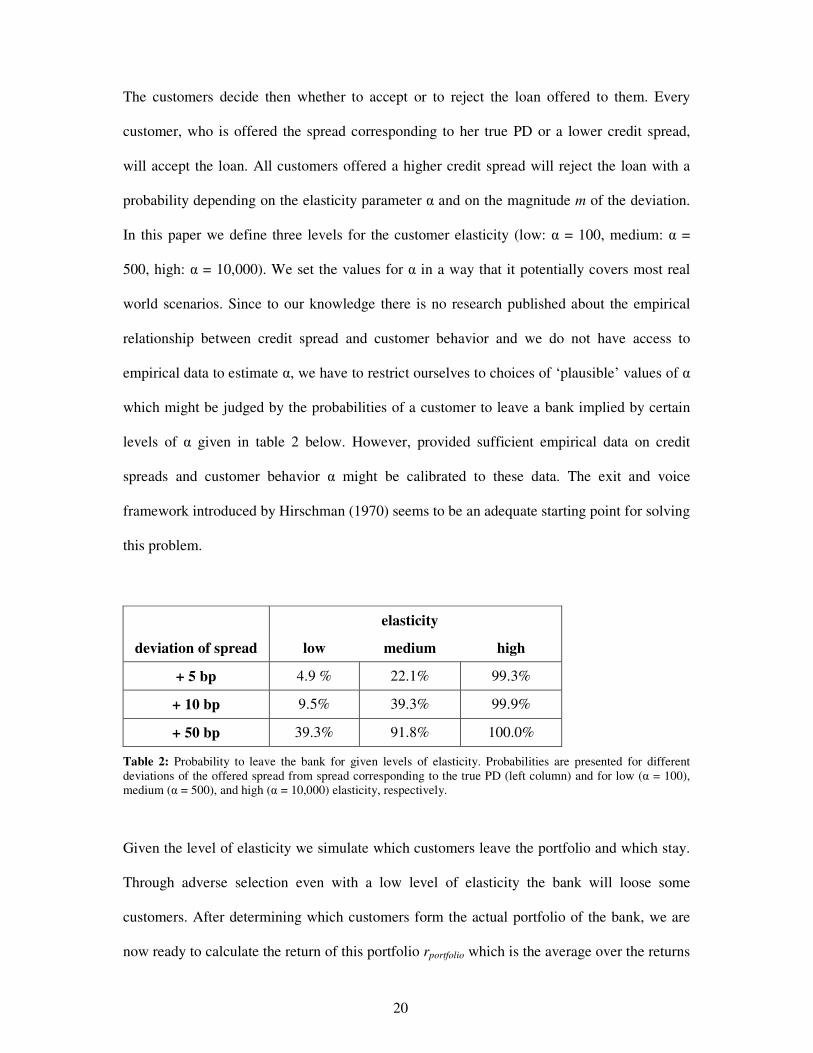
The customers decide then whether to accept or to reject the loan offered to them. Every

customer, who is offered the spread corresponding to her true PD or a lower credit spread,

will accept the loan. All customers offered a higher credit spread will reject the loan with a

probability depending on the elasticity parameter � and on the magnitude m of the deviation.

In this paper we define three levels for the customer elasticity (low: � = 100, medium: � =

500, high: � = 10,000). We set the values for � in a way that it potentially covers most real

world scenarios. Since to our knowledge there is no research published about the empirical

relationship between credit spread and customer behavior and we do not have access to

empirical data to estimate �, we have to restrict ourselves to choices of ‘plausible’ values of �

which might be judged by the probabilities of a customer to leave a bank implied by certain

levels of � given in table 2 below. However, provided sufficient empirical data on credit

spreads and customer behavior � might be calibrated to these data. The exit and voice

framework introduced by Hirschman (1970) seems to be an adequate starting point for solving

this problem.

elasticity

deviation of spread low medium high

+ 5 bp 4.9 % 22.1% 99.3%

+ 10 bp 9.5% 39.3% 99.9%

+ 50 bp 39.3% 91.8% 100.0%

Table 2: Probability to leave the bank for given levels of elasticity. Probabilities are presented for different deviations of the offered spread from spread corresponding to the true PD (left column) and for low (� = 100), medium (� = 500), and high (� = 10,000) elasticity, respectively.

Given the level of elasticity we simulate which customers leave the portfolio and which stay.

Through adverse selection even with a low level of elasticity the bank will loose some

customers. After determining which customers form the actual portfolio of the bank, we are

now ready to calculate the return of this portfolio rportfolio which is the average over the returns

21

on the individual loans ri (see equations 7 and 8). To calculate ri we simulate which customers

in the portfolio actually default using their individual true PDs. The return of the portfolio is

the result of one simulation path. For each combination of the parameters we run 100

simulations to estimate the average of the portfolio returns. These average returns are the

main results of our numerical analysis. We are able to examine the portfolio return effects for

different parameter constellations. The main task to compare rating systems with different

predictive power can now be achieved by simulating their returns in the proposed way.

4 Numerical results

In this section we quantify the effect of rating systems with different predictive power on the

portfolio return. Investing into a better rating system means to use more and better dispersed

rating cohorts and to reduce the measurement error in the estimation of the default

probabilities. In the first analysis we want to concentrate just on the effect of decreasing the

measurement error. To do this we define one base case:

Base Case: number of rating cohorts: 10

sizes of the rating cohorts: linearly increasing number of defaults (method 4)

number of customers: 10,000

LGD: medium (45%)

elasticity: medium (� = 500)

For this base case we quantify the effect on the portfolio return when improving the accuracy

of the PD estimation for the three different portfolios of different customer quality (see

section 3). In the first step the simulation approach of section 3 is used to estimate the

portfolio return for low accuracy (� = 2), medium accuracy (� = 0.5), high accuracy (� = 0.1),

22

and perfect accuracy (� = 0) given the parameter constellation of the base case. In the second

step the increase � of the portfolio return when using a rating system with medium, high, or

perfect accuracy level instead of a rating system with low accuracy level is calculated:

� medium = rportfolio, medium accuracy - rportfolio, low accuracy (9)

� high = rportfolio,high accuracy - rportfolio, low accuracy (10)

� perfect = rportfolio, perfect accuracy - rportfolio, low accuracy (11)

The increase � represents the potential gain in portfolio return for a bank when improving a

rating system with low accuracy to medium, high, or perfect accuracy. Table 3 shows the

increase � of the portfolio return when improving a rating system for the base case:

accuracy of PD estimation base case

medium high perfect

good portfolio 30.8 43.7 44.8

average portfolio 32.6 45.9 46.8

weak portfolio 39.0 56.4 58.7

Table 3: Increase in portfolio return (in bp) for the base case when improving the accuracy of the rating system from a low accuracy level (�=2) to a medium (�=0.5), high (�=0.1), or perfect (�=0) accuracy.

For realistic portfolios the return increases by 30 to 40 bp p.a. when the bank upgrades its

rating system from low to medium accuracy. Improving from medium to high accuracy

increases the portfolio return still by approximately 15 bp. Moving from high to perfect

accuracy results only in an approximate 1 bp improvement.

These results indicate that an improvement of the rating system has a very strong effect for

banks with low or medium accuracy systems. Avoiding the effect of adverse selection

improves the portfolio return significantly. The effect is also stronger for banks with rather

weak portfolios.

23

In the next step we present results of the portfolio return where the parameter values of our

base case are changed. We want to analyse if banks with certain characteristic in their

portfolio (e.g. highly collaterised loans) have more incentives to invest in their rating system.

In order to check for the influence of the degree of competitivity in the market environment

we change the elasticity parameter of the base case. One would expect that for banks with

more elastic customers, i.e. who leave the bank with higher probability if they are offered a

too high credit spread, the improvement of the rating system is more important. Table 4 and 5

show the increase � of the portfolio return when improving a rating system with low accuracy

to medium, high, or perfect accuracy in the case of high and low elasticity:

accuracy of PD estimation high elasticity

medium high perfect




Table 4: Increase in portfolio return (in bp) given high customer elasticity (�=10,000) when improving the accuracy of the rating system from a low accuracy level (�=2) to a medium (�=0.5), high (�=0.1), or perfect (�=0) accuracy.

accuracy of PD estimation low elasticity

medium high perfect




Table 5: Increase in portfolio return (in bp) for a low customer elasticity (�=100) when improving the accuracy of the rating system from a low accuracy level (�=2) to a medium (�=0.5), high (�=0.1), or perfect (�=0) accuracy.

24

The results clearly show that in loan markets with higher customer elasticity the improvement

is significantly stronger. In markets with oligopolistic structures and high market power for a

bank the adverse selection effect is not that important but still around 20 bp.

Next we analyse the effect of the LGD on the improvement potential of the rating system. We

compare portfolios with high LGD (75%) and low LGD (25%). We would expect that the

improvement of the rating system is more important for portfolios with high LGD. Table 6

and 7 show the increase � of the portfolio return when improving a rating system with low

accuracy to medium, high or perfect accuracy in the case of high and low LGD:

accuracy of PD estimation high LGD

medium high perfect




Table 6: Increase in portfolio return (in bp) for a high LGD (75%) when improving the accuracy of the rating system from a low accuracy level (�=2) to a medium (�=0.5), high (�=0.1), or perfect (�=0) accuracy.

accuracy of PD estimation low LGD

medium high perfect




Table 7: Increase in portfolio return (in bp) for a low LGD (25%) when improving the accuracy of the rating system from a low accuracy level (�=2) to a medium (�=0.5), high (�=0.1), or perfect (�=0) accuracy.

The results indicate that the LGD is very important for the size of the effect of improving

rating accuracy. Banks with low LGD, e.g. due to highly collaterised loans, do not depend

25

that much on the quality of their PD estimation. On the other side banks with completely

uncollaterised loans depend heavily on the accuracy of their PD estimation.

In the last analysis we compare the effect of rating accuracy for a different number of rating

cohorts. In the base case we used ten rating cohorts. Now we use five and infinitely many

ratings cohorts to analyse the effect.

accuracy of PD estimation five rating cohorts

medium high perfect




Table 8: Increase in portfolio return (in bp) for five rating cohorts when improving the accuracy of the rating system from a low accuracy level (�=2) to a medium (�=0.5), high (�=0.1), or perfect (�=0) accuracy.

accuracy of PD estimation infinitely many rating cohorts medium high perfect

Good portfolio 32.2 46.8 47.7


Weak portfolio 41.8 60.2 63.3

Table 9: Increase in portfolio return (in bp) for infinitely many rating cohorts when improving the accuracy of the rating system from a low accuracy level (�=2) to a medium (�=0.5), high (�=0.1), or perfect (�=0) accuracy.

As expected, the effect of rating accuracy is more important for banks that use more rating

cohorts. Banks that use a low number of rating cohorts have only a rough measure for the

PDs of the customers which are average default rates of coarse cohorts even if they can

measure individual PDs without error. Thus improving rating accuracy is not that important

for their situation.

26

5 Capital requirements

In this section we analyse the effect of improving the rating system on the regulatory capital

requirements of a bank. The Basel Committee on Banking Supervision previously has

released a series of consultative documents, accompanying working papers, and finally the

new capital adequacy framework commonly known as Basel II. One of the cornerstones of

this new Capital Framework ("Pillar 1") is a new risk-sensitive regulatory framework for a

bank's own calculation of regulatory capital for its credit portfolio. Banks which qualify

themselves in terms of data availability, statistical methods, risk management capabilities, and

a number of additional qualitative requirements will be allowed to adopt the Internal Rating

Based (IRB) approach to calculate their capital requirements. In the Foundation IRB (FIRB)

approach banks can use their own PD estimates of their customers. In the Advanced IRB

approach they can use own estimates of average loss rates and credit conversion factors

additionally.

We do not focus on institutional changes in regulatory capital related to differences in the

formulas for the risk weighted capital in the Modified Standardized Approach and the FIRB.

We concentrate rather on the economic value of improving a rating system given that a bank

has already qualified itself for the FIRB approach.

In the FIRB approach banks are allowed to use internal PD estimates to calculate the effect on

capital requirements for different rating systems using the proposed formulas suggested by the

Basel Committee. For expository purposes we concentrate on the formula for corporate

customers but the essence of our results will hold for other customer classes (retail, banks,

sovereigns) as well. The proposed capital requirement (CR) of a standard uncollateralized

27

corporate exposure expressed as a function of the customer's PD consists of two parts. The

first part represents the capital requirement for the unexpected loss (CR_UL):

( ))PD(b)5.2M(1)PD(b5.11

1

LGDPD)999.0(G)PD(R1

)PD(R)PD(G

)PD(R11

NLGD)PD(UL_CR

⋅−+⋅⋅−

⋅

⋅��

��

�⋅−��

�

��

�⋅

−+⋅

−⋅=

(12)

with

��

��

�

−−−⋅+

−−⋅= −

⋅−

−

⋅−

50

PD50

50

PD50

e1e1

124.0e1

e112.0)PD(R (13)

2))PDlog(05478.011852.0()PD(b ⋅−= (14)

where N(.) Standard normal cumulative distribution function

G(.) Standard normal inverse cumulative distribution function

LGD Loss-given-default; in the FIRB the LGD is set equal to 45% for standard

uncollateralized corporate exposures

PD For corporate exposures we have PD = max(PD*; 0.03%), where PD* denotes

the estimated PD of the customer

M Effective maturity; in the FIRB the effective maturity is set equal to 2.5 years.

The second part represents the capital requirement for the expected loss (CR_EL):

provisions eligible totalLGDPD)PD(EL_CR −⋅= (15)

28

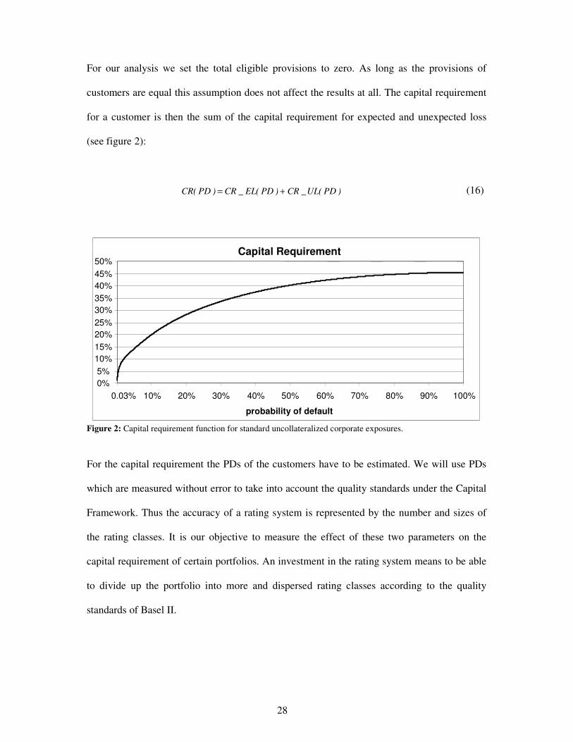
For our analysis we set the total eligible provisions to zero. As long as the provisions of

customers are equal this assumption does not affect the results at all. The capital requirement

for a customer is then the sum of the capital requirement for expected and unexpected loss

(see figure 2):

)PD(UL_CR)PD(EL_CR)PD(CR += (16)

Capital Requirement

0% 5% 10% 15% 20% 25% 30% 35% 40% 45% 50%

0.03% 10% 20% 30% 40% 50% 60% 70% 80% 90% 100%


Figure 2: Capital requirement function for standard uncollateralized corporate exposures.

For the capital requirement the PDs of the customers have to be estimated. We will use PDs

which are measured without error to take into account the quality standards under the Capital

Framework. Thus the accuracy of a rating system is represented by the number and sizes of

the rating classes. It is our objective to measure the effect of these two parameters on the

capital requirement of certain portfolios. An investment in the rating system means to be able

to divide up the portfolio into more and dispersed rating classes according to the quality

standards of Basel II.

29

Consider a rating class defined by an arbitrary PD interval. The capital requirement for this

rating class is obtained by

CR(E[PDi, i ∈ rating class]) (17)

where CR(.) denotes the capital requirment function and E[PDi, i ∈ rating class] denotes the

expected (or average) PD of rating class i. If the rating class i is divided into two non-empty

subclasses the capital requirement is given by

CR(E[PDj, j ∈ rating subclass 1]) + CR(E[PDk, k ∈ rating subclass 2]) (18)

The function to calculate the capital requirements out of the PDs, which is given in (12-16), is

strictly concave for PD values greater than the “floor” PD of 3 bp. As a consequence, it

follows from Jensen's inequality that

CR(E[PDi, i ∈ rating class]) > CR(E[PDj, j ∈ subclass 1]) + CR(E[PDk, k ∈ subclass 2])

(19)

Thus, having an iterative application of this argument in mind we conclude that the finer the

rating system the lower the regulatory capital requirement. In figure 3 we show the difference

in the capital requirements when we have two customers (A and B) and the PD is firstly

estimated for each customer and then the PD is estimated for the portfolio of the two

customers.

30

Capital Requirements

0% 5% 10% 15% 20% 25% 30% 35% 40% 45% 50%

0.03% 10% 20% 30% 40% 50% 60% 70% 80% 90% 100%


Customer B

Customer A

Capital requirements with separatePD estimation for A and B

Capital requirementswith PD estimation forthe portfolio of A and B

Figure 3: Consequences of Jensen's inequality on the calculation of the capital requirements.

From the theoretical point of view we can deduct that the structure of a rating system has a

potential impact on a financial institution's capital requirements. The main result based on

Jensen's inequality is that the finer the rating system, the lower the capital requirements.

However, we cannot deduct any indication about the potential size of these effects. To

provide such quantification we make more specific assumptions about the distribution of PDs

using the three different portfolios described in section 3.

Given the Beta density for all potential customers we can infer how many percent of the

customers in the portfolio have a PD inside the interval [x1, x2] and we can obtain the

expected PD for this group of customers analytically. This is all we need to know to calculate

the capital requirement for a set of rating cohorts where the corresponding cohort boundaries

are given by their minimal and the maximal PDs.

31

The expected value for the PD of a customer given that the customer has a PD between x1 and

x2 has the following functional form

[ ]),,(),,(

),,1(),,1(|

12

1221 xqpcdfxqpcdf

xqpcdfxqpcdfqp

pxPDxPDE

−+−+

⋅+

=≤≤ (20)

where cdf(.) denotes the cumulative density function of a Beta distribution with parameters p

and q. Provided this analytical relation we can avoid a simulation procedure compared to

section 4.

We calculate the capital requirement for the three portfolios under consideration using one,

two, five, ten, and infinitely many rating cohorts and using the four different methods to

construct credit score intervals (see appendix). Applying these methods of defining the sizes

of the rating classes the capital requirement for a different number of rating classes can be

compared. Tables 10 to 12 show the resulting capital requirements for the four methods over

the different PD distributions of our three portfolios:

good portfolio 1 cohort 2 cohorts 5 cohorts 10 cohorts � cohorts reduced capital requirements

using 10 instead of 5 cohorts

method 1 9.56% 9.55% 9.29% 8.84% 7.30% 45 bp

method 2 9.56% 7.91% 7.47% 7.36% 7.30% 11 bp

method 3 9.56% 8.94% 8.22% 7.87% 7.30% 35 bp

method 4 9.56% 8.63% 7.75% 7.48% 7.30% 27 bp

Table 10: Capital requirements for the good portfolio using one, two, five, ten, and infinitely many rating cohorts for different methods of defining the sizes of the rating cohorts.

32

average portfolio 1 cohort 2 cohorts 5 cohorts 10 cohorts � cohorts reduced capital requirements


method 1 9.37% 9.37% 9.25% 8.93% 8.00% 32 bp

method 2 9.37% 8.43% 8.11% 8.04% 8.00% 7 bp

method 3 9.37% 8.90% 8.46% 8.27% 8.00% 19 bp

method 4 9.37% 8.69% 8.21% 8.08% 8.00% 13 bp

Table 11: Capital requirements for the average portfolio using one, two, five, ten, and infinitely many rating cohorts for different methods of defining the sizes of the rating cohorts.

weak portfolio 1 cohort 2 cohorts 5 cohorts 10 cohorts � cohorts reduced capital requirements


method 1 9.99% 9.99% 9.95% 9.76% 9.25% 19 bp

method 2 9.99% 9.52% 9.33% 9.28% 9.25% 5 bp

method 3 9.99% 9.71% 9.48% 9.37% 9.25% 11 bp

method 4 9.99% 9.60% 9.36% 9.28% 9.25% 8 bp

Table 12: Capital requirements for the weak portfolio using one, two, five, ten, and infinitely many rating cohorts for different methods of defining the sizes of the rating cohorts.

Using more and better dispersed rating classes a bank can save a significant amount of

regulatory capital. Depending on the portfolio and on the method of defining the sizes of the

rating classes the capital requirements can be reduced by up to 45 bp when using ten instead

of five rating classes. On average a bank which increases the number of rating classes from

five to ten can expect a lower capital requirement of around 10 to 20 bp. Increasing the

number of rating classes from ten to infinity can still be important for certain methods of

defining the rating classes. However, for more sophisticated methods (e.g. method 2) the

effect is comparably small (around 3 bp). Analysing the results of the capital requirement for

the different methods of defining the sizes of rating classes we conclude that method 2 (equal

number of customers per rating class) and method 4 (linearly increasing number of expected

defaults per rating class) are the most promising concepts. The magnitude of the differences

between these two methods is rather small. Method 1 (equally spaced PD intervals) and

method 3 (equal number of expected defaults) consistently yielded higher regulatory capital

33

requirements than the others. We explain this outcome by the fact that method 1 and 3 yield

comparably broad cohorts for customers with low PDs. Since the relative frequency of low

PDs is high for all portfolios under consideration method 1 and 3 produce a rather crude

rating system in this setup which implies higher capital requirements due to the concaveity of

the Basel risk-weight function.

In order to compare the magnitude of the economic value of reduced capital requirements one

has to convert these figures into annual returns by multiplying the reduction in capital

requirement with the costs of capital, e.g. a reduction of 20 bp in regulatory capital multiplied

by 15% costs of capital translates into a 3 bp increase in the annual return. Compared to the

effect of adverse selection the potential of this effect seems to be much lower.

6 Conclusion

In this paper we develop a model to determine the potential economic value of improving a

credit rating system. We describe a credit rating system by the number and sizes of the rating

classes and the measurement error in the estimation of individual default probabilities. Our

model is aimed to advise banks when making an investment decision with respect to the

quality of their rating systems. All model parameters are designed to be empirically

observable or at least to be calibrated to empirically observable values.

In a first step we analyze the potential effect of adverse selection on the credit portfolio return

for rating systems with different accuracy. Our findings indicate that improving a rating

system with low accuracy to medium accuracy can increase the annual rate of return by 30 to

40 bp. This effect is even stronger for banks operating in markets with high customer

34

elasticity and high loss rates. Compared to the estimated implementation costs banks could

have a strong incentive to invest into their rating system.

Our analysis is restricted to a partial equilibrium framework. Including two or more

representative lenders with different rating systems and different implementation costs and

modelling the dynamic strategic competition between the lenders would potentially provide

more insight to the real-world decision problems banks currently are facing. The framework

presented in this paper thus describes the basic decision model that might be used as a starting

point in a more sophisticated dynamic setup where modelling the cost differentials of

implementing and maintaining rating systems among banks will play a crucial role.

In a second step we analyse the effects of the reduction of regulatory capital requirements

under the Basel FIRB approach. Improving the accuracy or rating systems gives the bank the

opportunity to make use of a finer grained rating system, i.e. to use a higher number of rating

classes. The concaveity of the regulatory capital formula implies that capital requirements are

lower for finer grained rating systems. Our results show that the potential of this effect on the

portfolio return is rather weak compared to the effect of adverse selection.

35

References

Accenture, Mercer Oliver Wyman, and SAP, 2004, Reality Check on Basel II, Special

Supplement to The Banker, July 2004, 152-161.

Basel Committee on Banking Supervision, 2004, International Convergence of Capital

Measurement and Capital Standards: a Revised Framework, Basel, June 2004, www.bis.org.

Broecker, T., 1990, Credit-Worthiness Tests and Interbank Competition, Econometrica 58/2,

429-452.

Duffie, D., Singleton, K., 1999, Modeling term structures of defaultable bonds, Review of

Financial Studies 12 (4), 197 - 226

Fudenberg, D., Tirole, J., 1985, Preemption and Rent Equalization in the Adoption of a New

Technology, Review of Economic Studies 52/3, 383-401.

Gross, T., Kolbeck, C., Nicolai, A., Rockenfelt, M., 2002, Deutsche Banken auf dem Weg zu

Basel II, Research Report, Boston Consulting Group and University of Witten/Herdecke.

Hirschman, A.O., 1970, Exit, Voice, and Loyalty. Responses to Decline in Firms,

Organizations, and States., Cambridge / Mass., Harvard University Press.

Jarrow, R., Lando, D., Turnbull, S., 1997, A Markov model for the term structure of credit

risk spreads, Review of Financial Studies 10 (2), 481 – 523.

36

Jordão, F., Stein, R., 2003, What is a more powerful model worth? Moody’s – KMV

Technical report #030124.

Krahnen, J.P., Weber, M., 2001, Generally accepted rating principles: A primer, Journal of

Banking & Finance, 25 (1), 3 – 23.

Lando, D., Skodeberg, T., 2002, Analyzing rating transitions and rating drift with continuous

observations, Journal of Banking & Finance, 26 (2/3), 423 – 444.

Renault, O., Scaillet, O., 2003, On the way to recovery: A nonparametric bias free estimation

of recovery rate densities, FAME Research Paper No. 83, HEC Geneve.

Schwaiger, W., 2003, Basle II: Quantitative impact study on small and medium-sized

enterprises in Austria, in: Chen et al. (Editors): The Role of International Institutions in

Globalisation: The Challenges of Reform, Edgar Elgar, pp. 166 – 180.

Treacy, W. F., Carey, M., 2000, Credit rating systems at large US banks, Journal of Banking

& Finance, 24 (1/2), 167 – 201.

37

Appendix

Concerning the sizes of the rating classes there is no natural best solution to define PD

boundaries. Once the borrowers have been sorted from lowest to highest according to

estimated PD, boundary PDs are chosen using one of four methods:

Method 1: The maximal PD for the worst customer is taken and divided by the numbers of

cohorts. The resulting value is the stepsize for setting the boundaries.

Example: The maximal PD in a portfolio is 50%. In the case of five cohorts this number

is divided by 5 resulting in a stepsize of 10%. So the PD intervals are:

0% - 10%, 10% - 20%, 20% - 30%, 30% - 40%, 40% - 50%.

Method 2: The boundaries are set such that every cohort has the same number of customers.

Example: For 5 cohorts 20% of the customers are in each cohort.

Method 3: The boundaries are set such that every cohort has the same number of defaults.

Example: For 5 cohorts 20% of the defaults are in each cohort.

Method 4: The boundaries are set such that the number of defaults increases linearly from the

best to the worst cohort. In this case we have the following relations:

38

iAi =⋅ ξ (21)

11

==

k

iiA (22)

with i index of the cohort

Ai percentage of all defaults in cohort i

k number of cohorts

which are solved for �:

)1(

2+⋅

=kk

ξ (23)

Once we know � we can use the first equation to calculate how many defaults are in each

cohort and with this the boundaries can be calculated.

Example: For five cohorts � is equal to:

6760,0151

)15(52 ==

+⋅=ξ

Consequently all defaults are distributed over the cohorts as follows:

cohort 1: 6.67% of all defaults are in this cohort


cohort 3: 20% of all defaults are in this cohort



Date post:	23-Feb-2022
Category:	Documents
Upload:	others
View:	4 times
Download:	0 times

Modelling the Economic Value of Credit Rating Systems

Documents