Page 1
MODELLING THE OPTIMUM INTERFACE BETWEEN OPEN PIT
AND UNDERGROUND MINING FOR GOLD MINES
Seth Opoku
A thesis submitted to the Faculty of Engineering and the Built Environment, University
of the Witwatersrand, Johannesburg, in fulfilment of the requirements for the degree of
Doctor of Philosophy.
Johannesburg 2013
Page 2
i
DECLARATION
I declare that this thesis is my own unaided work. Where use was made of the work of
others, it was duly acknowledged. It is being submitted for the Degree of Doctor of
Philosophy in the University of the Witwatersrand, Johannesburg. It has not been
submitted before in any form for any degree or examination at any other university.
Signed
……………………………..
(Seth Opoku)
This……………….day of……………..………2013
Page 3
ii
ABSTRACT
The open pit to underground transition problem involves the decision of when, how and
at what depth to transition from open pit (OP) to underground (UG). However, the
current criteria guiding the process of the OP – UG transition are not well defined and
documented as most mines rely on their project feasibility teams’ experiences. In
addition, the methodologies used to address this problem have been based on
deterministic approaches. The deterministic approaches cannot address the
practicalities that mining companies face during decision-making, such as uncertainties
in the geological models and optimisation parameters, thus rendering deterministic
solutions inadequate.
In order to address these shortcomings, this research reviewed the OP – UG transition
problem from a stochastic or probabilistic perspective. To address the uncertainties in
the geological models, simulated models were generated and used. In this study,
transition indicators used for the OP - UG transition were Net Present Value (NPV),
ratio of price to cost per ounce of gold, stripping ratio, processed ounces and average
grade at the run of mine pad. These indicators were used to compare four individual
case study mines; with AngloGold Ashanti’s Sunrise Dam Gold Mine in Australia, which
made the OP – UG transition in 2004 and hence develop an OP – UG transition model.
Sunrise Dam Gold Mine is a suitable mine for providing baseline values because it
recently made the OP-UG transition. Only four case study mines were used because it
took nine months to generate transition indicators for each case study mine.
A generic model was developed from the results of the four case studies to help mining
companies make the OP - UG transition decision. The model uses a set of transition
indicators that trigger the decision while recognising the uncertainties in the geological
models, future mineral price as well as cost and processing parameters. From the
generic model, mines can transition when the margin (gold price to cost per ounce
ratio) is greater than 2.0; grade is between 4 g/t and 9 g/t, stripping ratio between 3 and
15 m3/t and positive NPV depending on the type of deposit. With this model mines can
now transition when the critical conditions of the transition indicators (gold price to cost
per ounce, grade and stripping ratio) are achieved. The model also uses the set of
transition indicators to model the probabilistic nature of the OP-UG interface. The
derived generic model will help mining companies in their annual reviews to assess the
OP - UG interface and make decisions early enough with regard to transition timing.
Page 4
iii
PUBLISHED WORK
The publications listed below have emanated from this research work so far:
Opoku, S and Musingwini, C. (2012), Modelling geological uncertainty for open-
pit to underground transition in gold mines, in Proceedings of the 21st
International Symposium on Mine Planning and Equipment Selection (MPES
2012), 28th–30th November 2012, New Delhi, India.pp. 503-512.
Opoku, S and Musingwini, C. (2013), Stochastic modelling of open pit to
underground transition interface for gold mines, a paper accepted for
publication in the International Journal of Mining, Reclamation and
Environment.
Page 5
iv
ACKNOWLEDGEMENTS
I wish to thank God almighty for giving me life, knowledge and opportunity to author
this document. I am indebted to AngloGold Ashanti Limited for the permission given to
use some of their mines as case studies and software for this thesis. In addition, I
would like to particularly acknowledge the following individuals for their specific
contributions:
Professor Cuthbert Musingwini (University of Witwatersrand), my supervisor for
his contribution, support and guidance throughout the thesis;
My mentor, Mr. Alex Bals (Vice President AngloGold Ashanti), for his invaluable
support and advice;
Mr. Vaughan Chamberlain (Senior Vice President AngloGold Ashanti), Mr.
Richard Peattie (General Manager AngloGold Ashanti) and Mr. Tom Gell (Vice
President AngloGold Ashanti) for providing support and permission to use the
company’s geological models;
Mr. Silva Alessandro Henrique Medeiros, Mr. Isaac Nino (Ingeniero Senior
Projectos Avanzados), Aballay Soria Raúl (CVSA), Mr. Sissoko Adama
(Evaluation Manager Geita Gold Mine), Belinda Roux (Senior Information
Officer AngloGold Ashanti) and Abigail Maile for providing some of the
background research for the thesis;
Mr. Jason May (Senior Vice President AngloGold Ashanti), Mr. Jamie
Williamson, Mr. Mark Kent and Mr. Ouedraogo Didier all of AngloGold Ashanti
for assisting in creating the simulated models using Isatis;
Mr. Richard Thomas (Vice President AngloGold Ashanti), Mr. Michael Birkhead
(Senior Vice President AngloGold Ashanti), Mr. Desiderius Kamugisha and
Alistides Ndibalema (Senior Mining Engineers AngloGold Ashanti) for validation
and peer review of the macros and optimisation parameters. Mr. Lloyd
Flanagan (Hydro geologist Superintendent AngloGold Ashanti) for proofreading
the draft chapters.
Professor Roussos Dimitrakopoulos, Professor Raymond Suglo, Mr. R.M. Kear
and Mr. Paul Lindsay for their professional advice, discussions on the mining
industry, and for sharing their experiences; and
Finally, my greatest thanks go to my family especially my wife, Rev. Victoria
Opoku Achiamaa for the sacrifices, prayers and words of encouragement
during difficult times.
Page 6
v
Although the opportunity and permission to use some of the material contained in this
thesis is gratefully acknowledged, the opinions expressed are those of the author and
may not necessarily represent the policies of the companies mentioned. Any errors and
ambiguities in this thesis are entirely my own responsibility.
Page 7
vi
TABLE OF CONTENTS
DECLARATION ............................................................................................................ i
ABSTRACT ................................................................................................................. ii
PUBLISHED WORK ....................................................................................................iii
ACKNOWLEDGEMENTS ............................................................................................iv
TABLE OF CONTENTS ...............................................................................................vi
ABBREVIATIONS.................................................................................................... xviii
1.0 INTRODUCTION .................................................................................................. 1
1.1 Background information ...................................................................................... 4
1.1.1 Status of some open pit to underground transition mines ............................. 5
1.1.2 Related research and choice of gold mines as case studies ........................ 6
1.2 Research question .............................................................................................. 7
1.3 Statement of objectives of the thesis .................................................................. 8
1.4 Research methodology ....................................................................................... 8
1.5 Problem formulation ........................................................................................... 8
1.6 Thesis structure .................................................................................................. 9
2.0 REVIEW OF OPEN PIT TO UNDERGROUND TRANSITION .............................11
2.1 Previous research on open pit to underground transition ...................................12
2.1.1 Cost and stripping ratio ...............................................................................12
2.1.2 Transition depth and its determination ........................................................14
2.1.3 Geotechnical challenges .............................................................................17
2.1.4 Going underground .....................................................................................19
2.1.5 Evaluation of technical and economic criteria involved in changing from
surface to underground mining ............................................................................21
2.1.6 Underground mining: a challenge to established open pit operations ..........24
2.2 Using Whittle software to determine when to go underground ...........................24
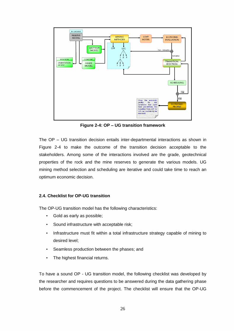
2.3. OP –UG transition framework ...........................................................................25
2.4. Checklist for OP-UG transition ..........................................................................26
2.4.1 Geology ......................................................................................................27
Page 8
vii
2.4.2 Operational .................................................................................................27
2.4.3 Geotechnical ...............................................................................................28
2.5 Chapter summary ..............................................................................................29
3.0 PROCESS FOR MODELLING OPEN PIT TO UNDERGROUND TRANSITION .30
3.1 Processes followed in the creation of OP-UG transition model ..........................30
3.1.1 Model preparation for simulation .................................................................31
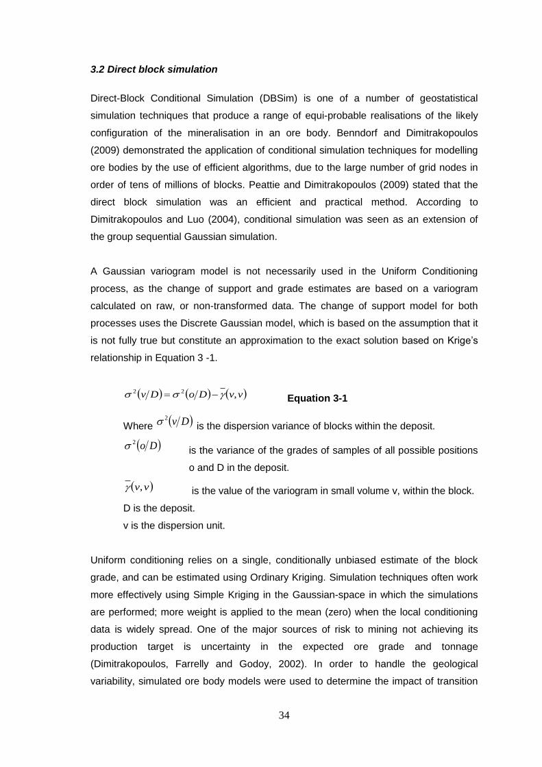
3.2 Direct block simulation .......................................................................................34
3.2.1 Quality control and simulation data coverage ..............................................36
3.3 Methodology for creating simulated models .......................................................36
3.3.1 Problems encountered in simulated models creation ..................................38
3.4 Preparation of simulated models for pit optimisation ..........................................39
3.5 Optimisation of open pit and underground mining ..............................................40
3.6 Mineable Reserve Optimiser processes ............................................................44
3.7 Scheduling using XPAC software ......................................................................44
3.8 The validity of software used for OP-UG transition ............................................46
3.9 Conceptual OP-UG transition model ..................................................................47
3.10 Guide for OP-UG transition for gold mines and how to incorporate geological
uncertainty in the transition ......................................................................................48
3.11 Chapter summary ............................................................................................49
4.0 DESCRIPTION OF CASE STUDIES: OPEN PIT - UNDERGROUND
TRANSITION ..............................................................................................................50
4.1 CASE STUDY 1: GEITA GOLD MINE ...............................................................50
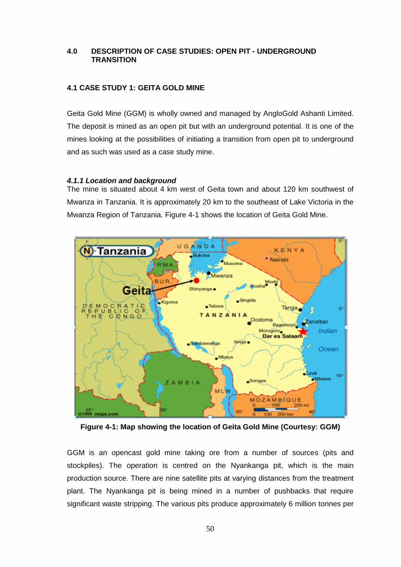
4.1.1 Location and background ............................................................................50
4.1.2 History of Geita Gold Mine ..........................................................................52
4.1.3 Geology and ore body properties ................................................................53
4.1.4 Transition plans ..........................................................................................56
4.2 CASE STUDY 2: CERRO VANGUARDIA SA MINE ..........................................57
4.2.1 Location and background ............................................................................58
4.2.2 History of CVSA Mine .................................................................................61
4.2.3 CVSA geology and transition plans .............................................................61
Page 9
viii
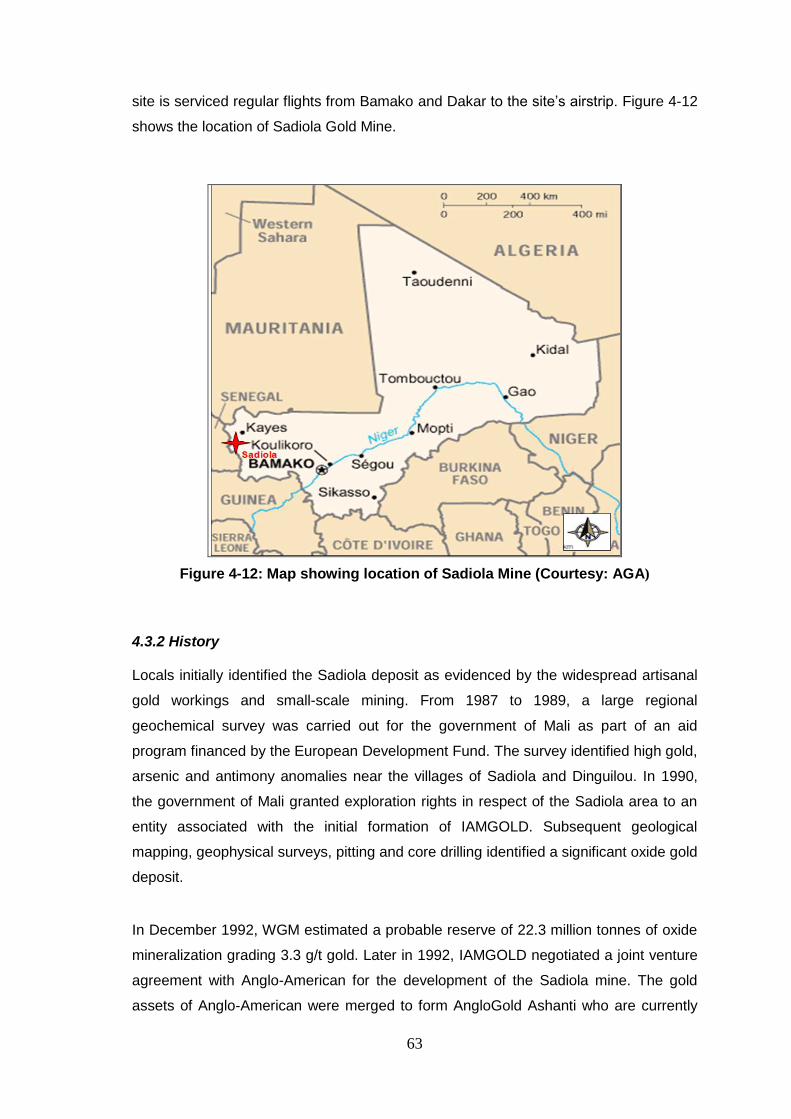
4.3 CASE STUDY 3: SADIOLA GOLD MINE...........................................................62
4.3.1 Location and background ............................................................................62
4.3.2 History ........................................................................................................63
4.3.3 Geology, current plans and production .......................................................64
4.3.4 Transition plans ..........................................................................................66
4.4 CASE STUDY 4: MORILA GOLD MINE ............................................................66
4.4.1 Location and background ............................................................................67
4.4.2 History ........................................................................................................68
4.4.3 Geology, current plans and production .......................................................68
4.4.4 Transition plans ..........................................................................................70
4.5 CHAPTER SUMMARY ......................................................................................72
5.0 BASELINE VALUES FOR MODEL USING SUNRISE DAM GOLD MINE AS
BENCHMARK .............................................................................................................73
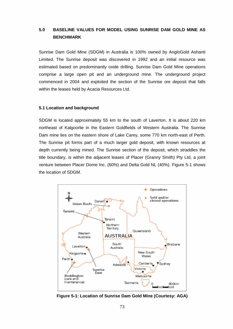
5.1 Location and background ..................................................................................73
5.2 History ...............................................................................................................74
5.3 The use of SDGM for benchmarking against mining industry ............................75
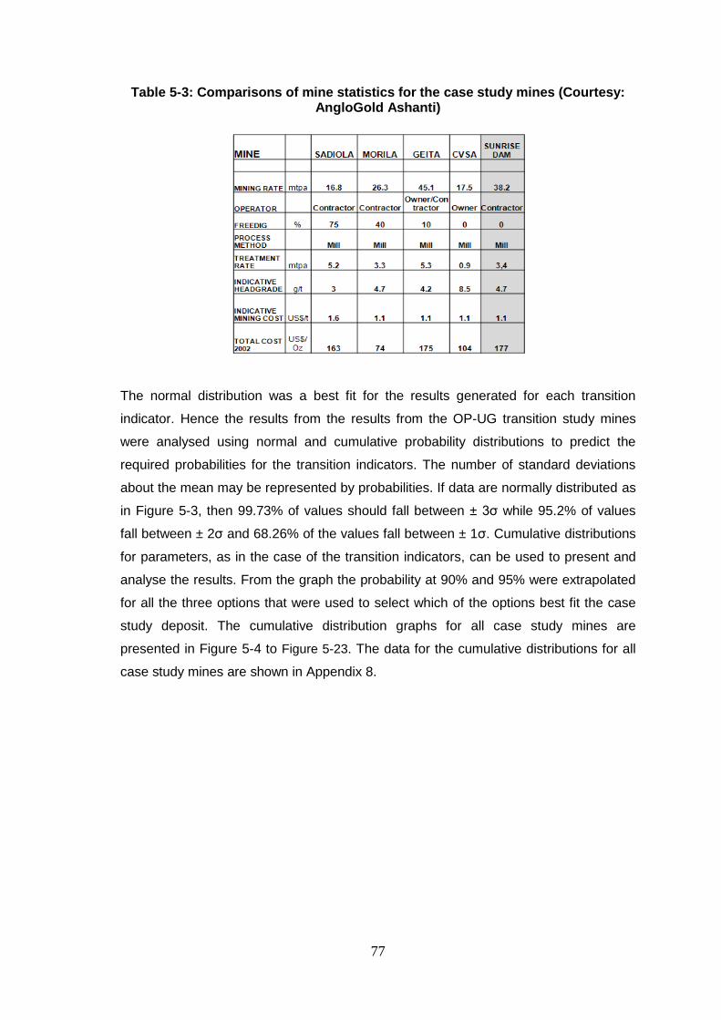
5.4 Analysis and interpretation of the results ...........................................................76
5.5 OP - UG transition model baseline results .........................................................91
5.6 Chapter summary ............................................................................................ 101
6.0 CONCLUSIONS AND RECOMMENDATIONS .................................................. 102
6.1 Conclusions ..................................................................................................... 102
6.2 Research contribution and limitations .............................................................. 102
6.3 Recommendations for future research ............................................................. 103
7.0 REFERENCES .................................................................................................. 104
APPENDICES ........................................................................................................... 109
Appendix 1: Fields in geological block models ....................................................... 109
Geita .................................................................................................................. 109
Sadiola .............................................................................................................. 109
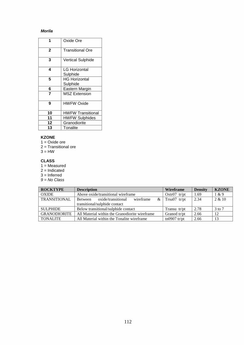
Morila ................................................................................................................ 112
Page 10
ix
Appendix 2: Model checking and preparation macros ............................................ 113
Macros for checking models before simulation .................................................. 113
Macro to prepare models after simulation .......................................................... 113
Macros for Whittle inputs preparation ................................................................ 117
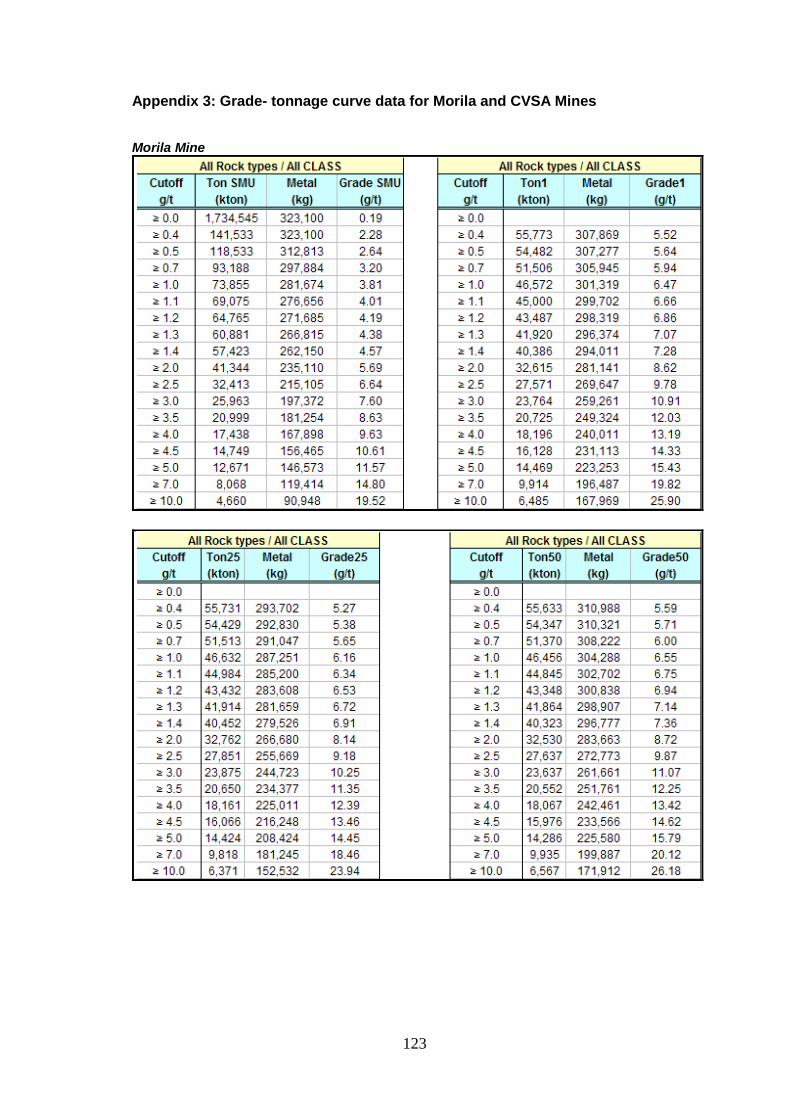
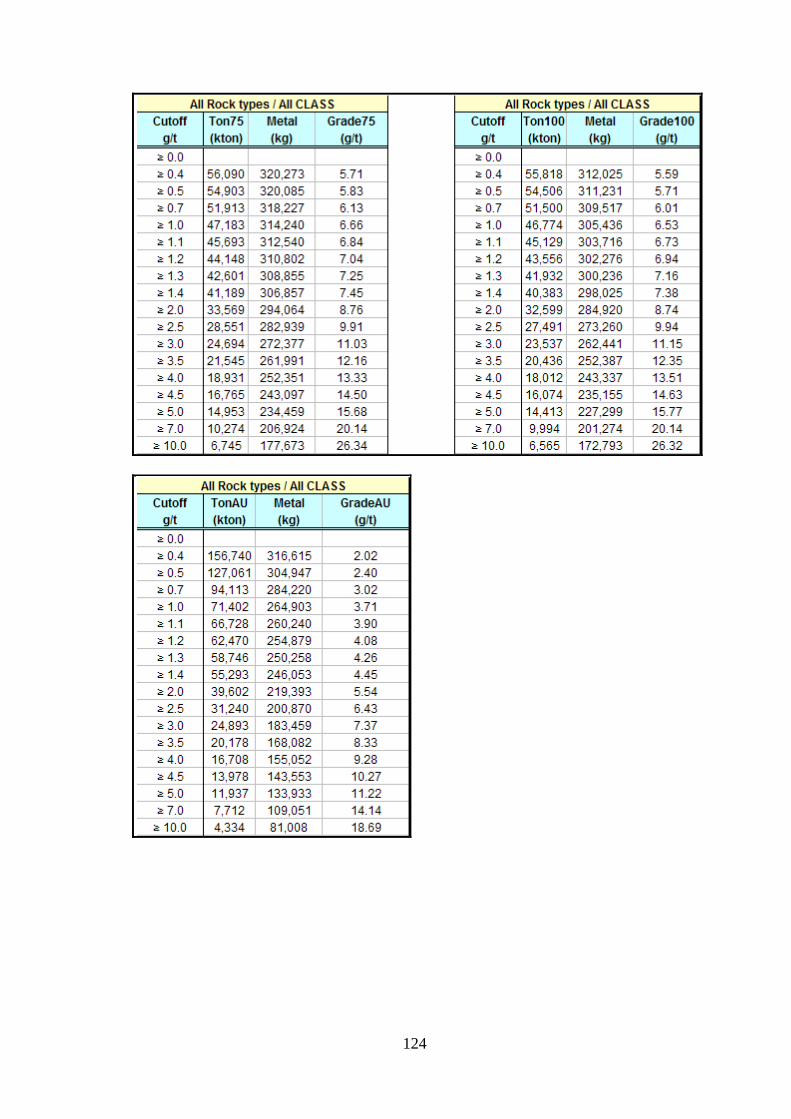
Appendix 3: Grade- tonnage curve data for Morila and CVSA Mines ..................... 123
Morila Mine ........................................................................................................ 123
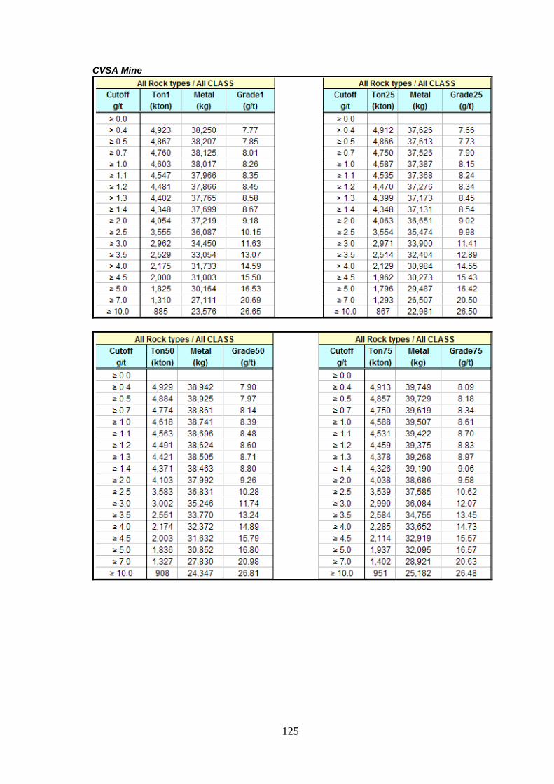
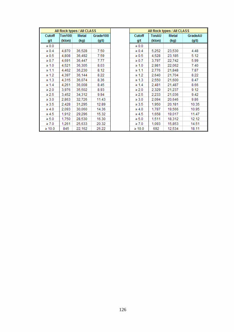
CVSA Mine ........................................................................................................ 125
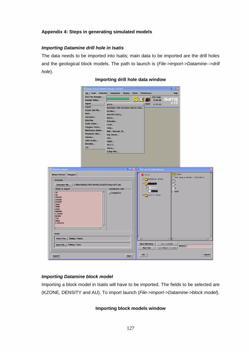
Appendix 4: Steps in generating simulated models ............................................... 127
Importing Datamine drill hole in Isatis ................................................................ 127
Importing Datamine block model ....................................................................... 127
Creating intervals for selection ........................................................................... 128
Creating Isatis grid ............................................................................................. 128
Migration of Datamine parameters to Isatis grid ................................................. 129
Creating selection with Isatis grid ...................................................................... 130
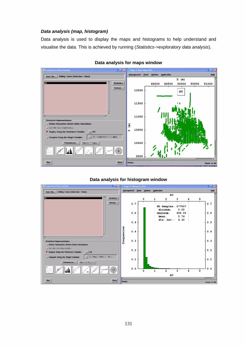
Data analysis (map, histogram) ......................................................................... 131
Exploratory data analysis-point anamorphosis ................................................... 132
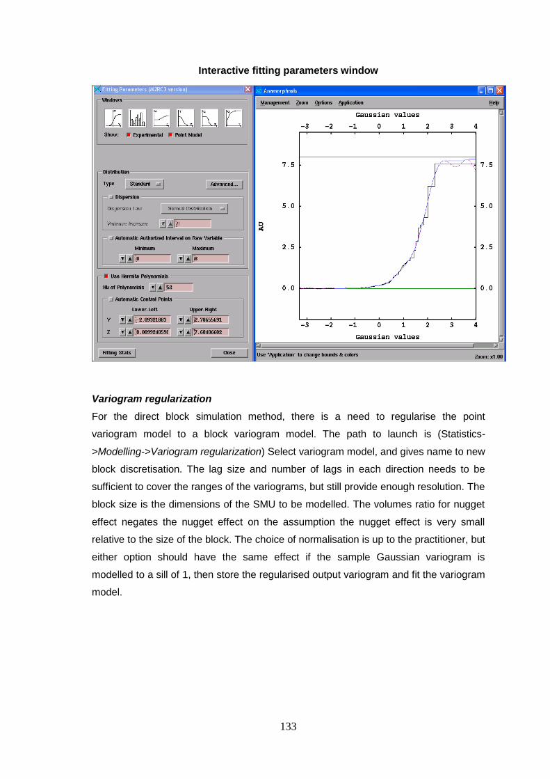
Variogram regularization .................................................................................... 133
Block variogram fitting ....................................................................................... 134
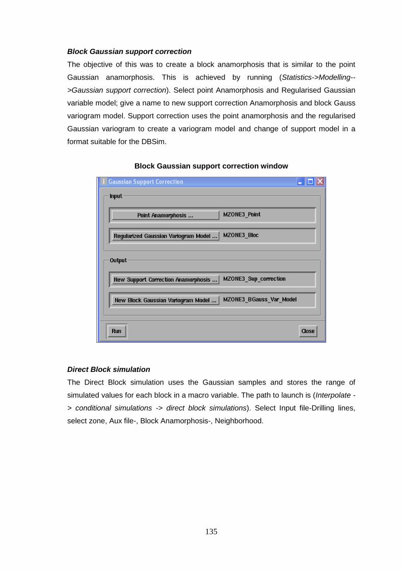
Block Gaussian support correction .................................................................... 135
Direct Block simulation ...................................................................................... 135
Exporting simulated model to Datamine format.................................................. 136
Appendix 5: MRO Datamine script and input parameters ...................................... 137
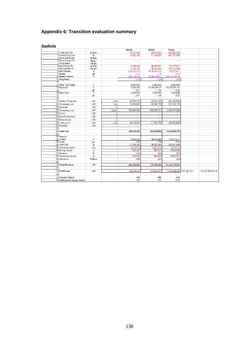
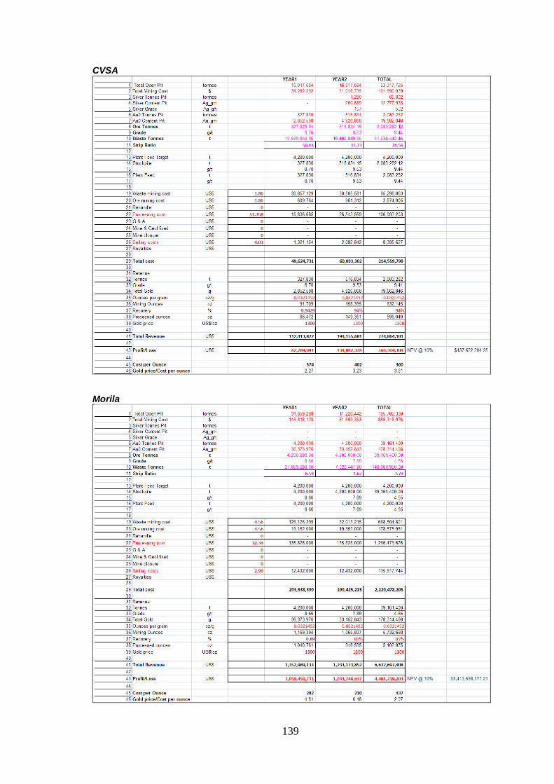
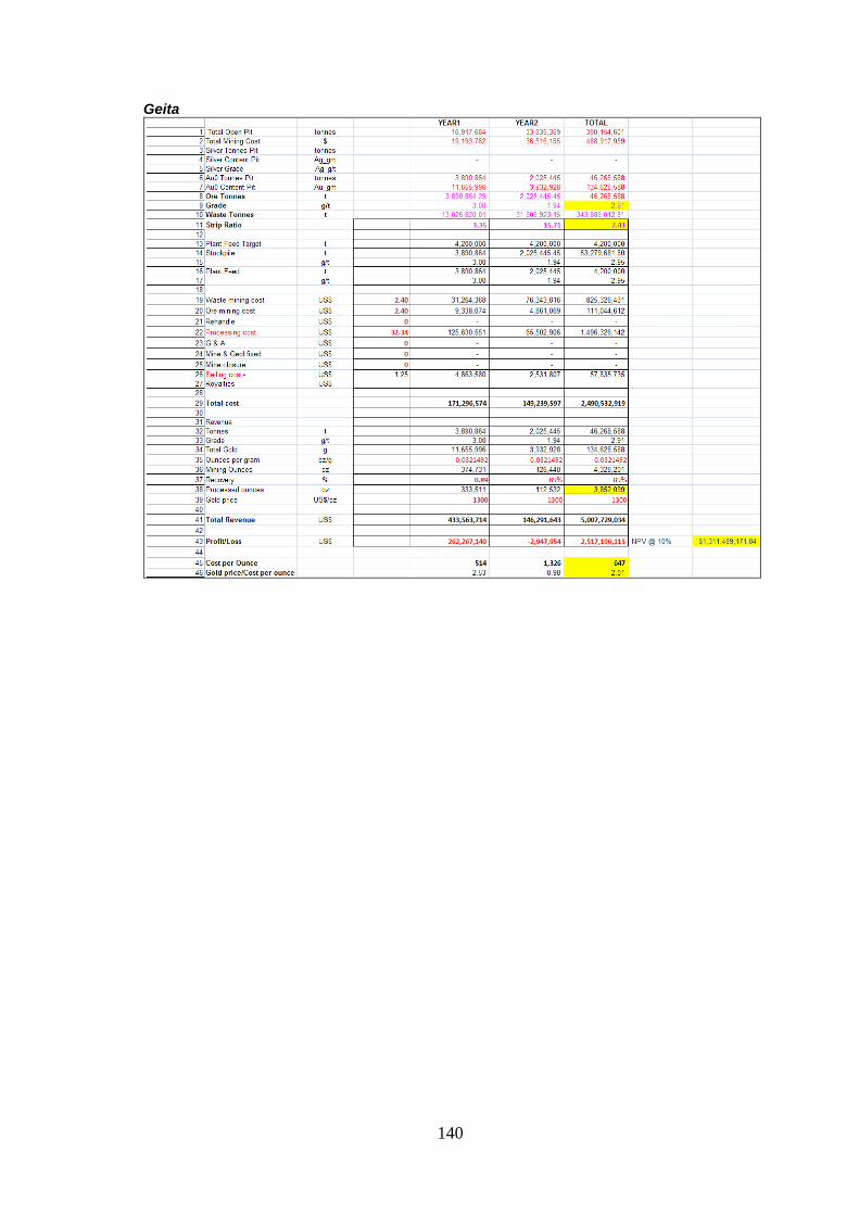
Appendix 6: Transition evaluation summary .......................................................... 138
Sadiola .............................................................................................................. 138
CVSA ................................................................................................................ 139
Morila ................................................................................................................ 139
Geita .................................................................................................................. 140
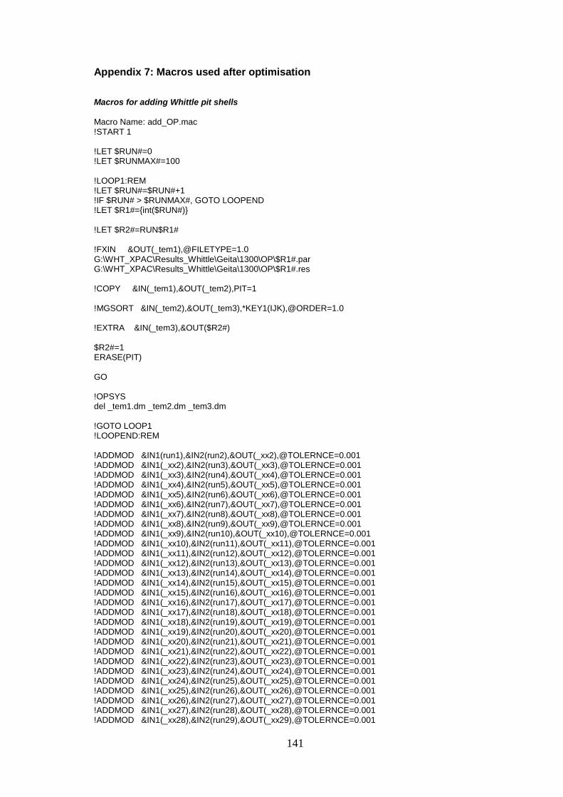
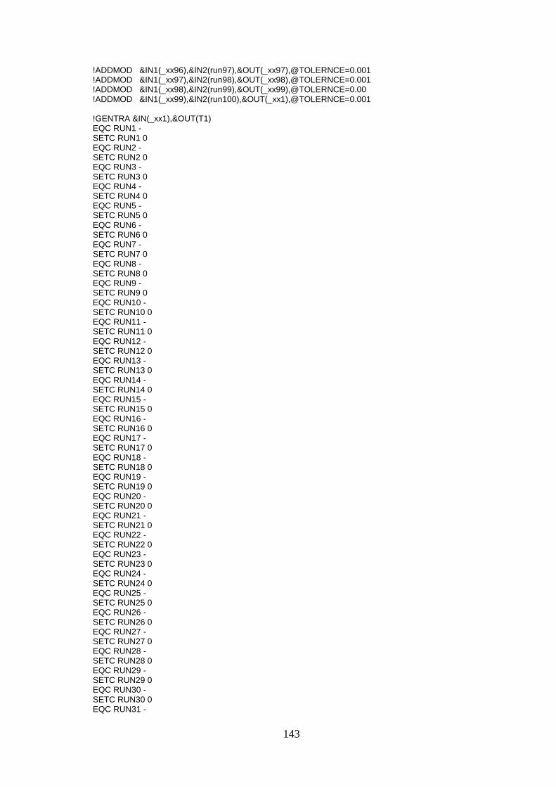
Appendix 7: Macros used after optimisation .......................................................... 141
Macros for adding Whittle pit shells ................................................................... 141
Page 11
x
Macros for converting block models to wireframes ............................................ 150
Macros for creating pushbacks .......................................................................... 152
Macros to create input models for evaluation (XPAC) ........................................ 152
XPAC preparation macros ................................................................................. 153
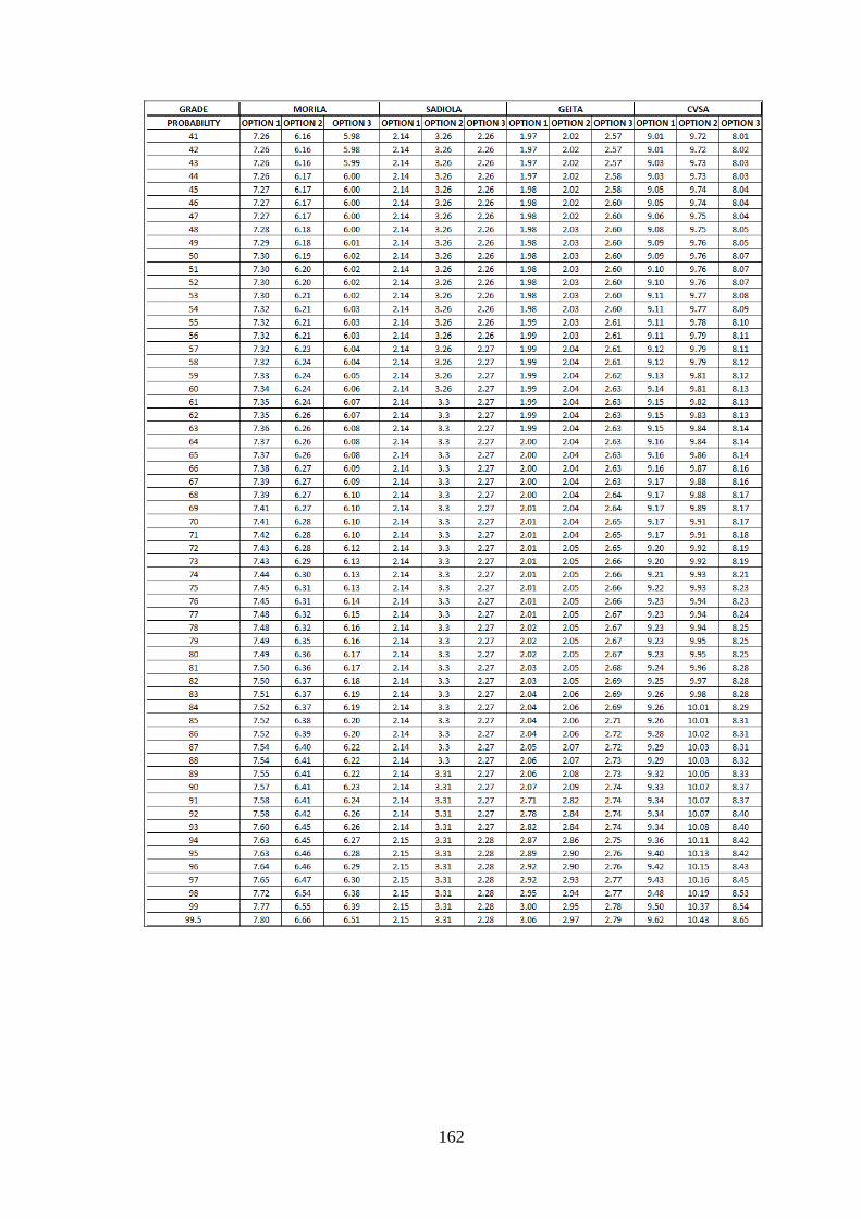
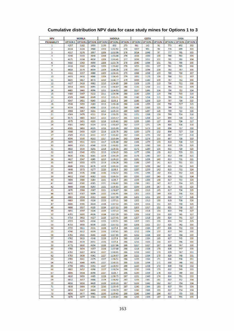
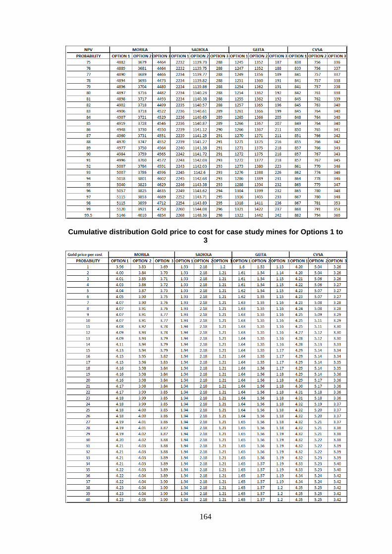
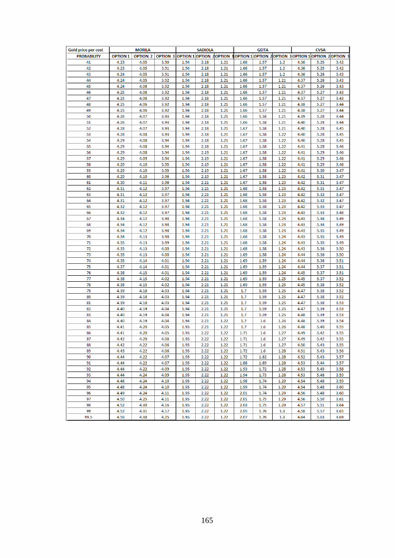
Appendix 8: Cumulative distribution data for Geita, Sadiola and Morila Mines ....... 160
Cumulative distribution processed ounces data for case study mines for Options 1
to 3 .................................................................................................................... 160
Cumulative distribution Grade data for case study mines for Options 1 to 3 ...... 161
Cumulative distribution NPV data for case study mines for Options 1 to 3 ......... 163
Cumulative distribution Gold price to cost for case study mines for Options 1 to 3
.......................................................................................................................... 164
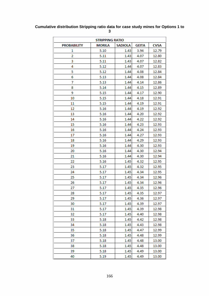
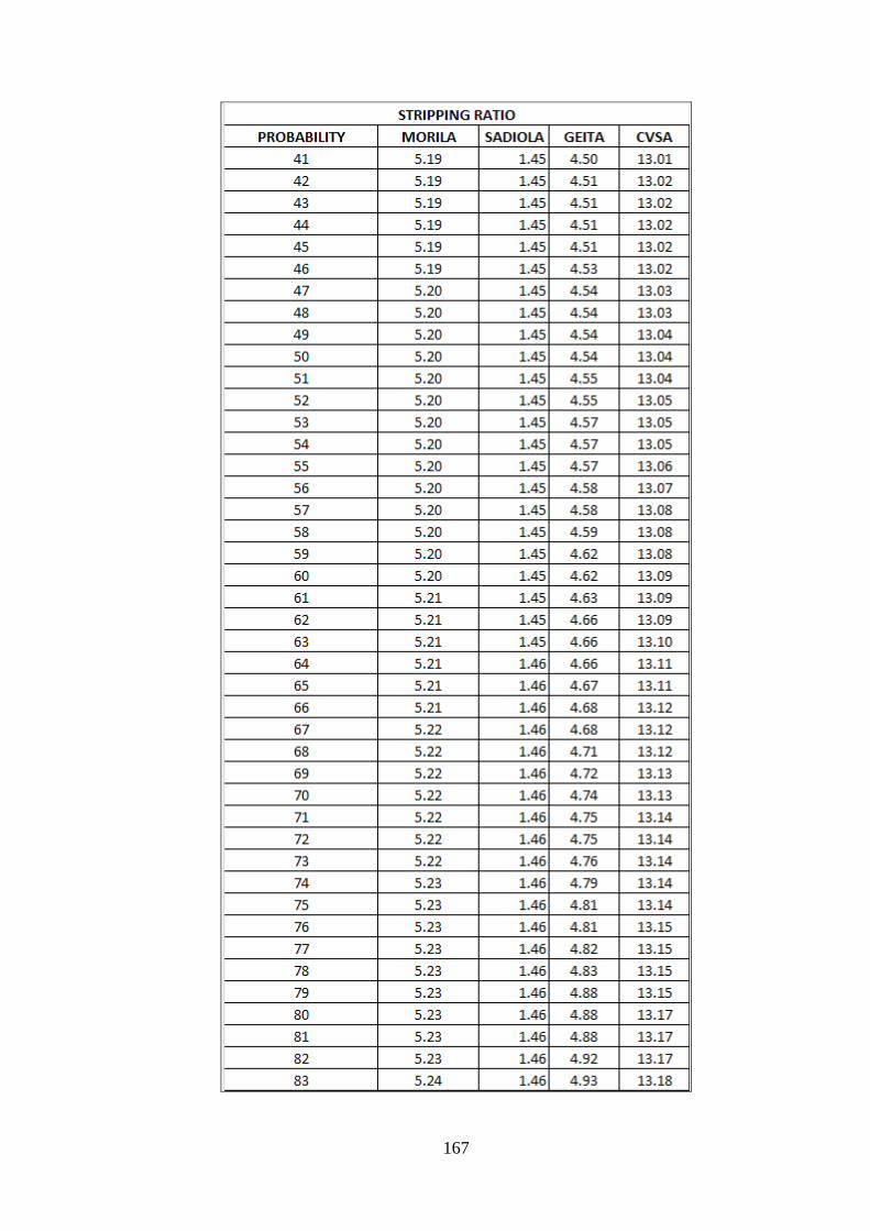
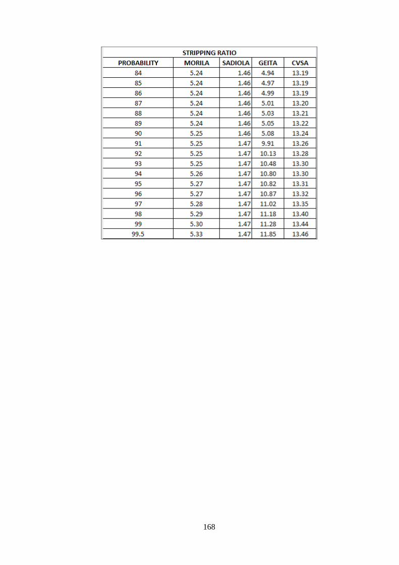
Cumulative distribution Stripping ratio data for case study mines for Options 1 to 3
.......................................................................................................................... 166
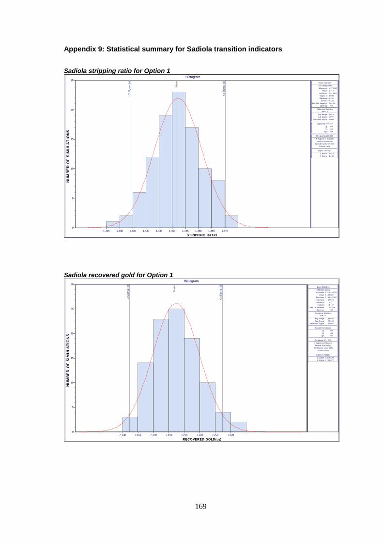
Appendix 9: Statistical summary for Sadiola transition indicators........................... 169
Sadiola stripping ratio for Option 1 ..................................................................... 169
Sadiola recovered gold for Option 1................................................................... 169
Sadiola recovered gold for Option 3................................................................... 170
Sadiola recovered grade for Option 1 ................................................................ 170
Sadiola recovered grade for Option 2 ................................................................ 171
Sadiola recovered grade for Option 2 Bi-modal option 1 .................................... 171
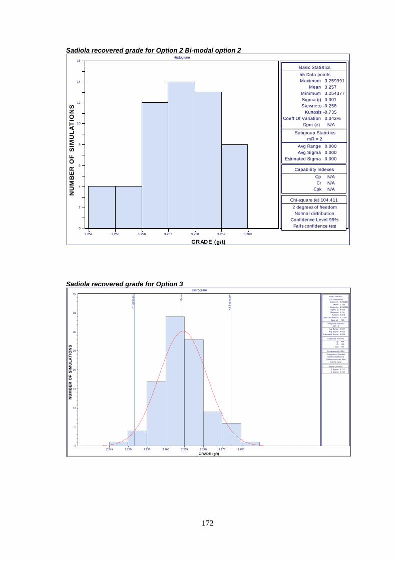
Sadiola recovered grade for Option 2 Bi-modal option 2 .................................... 172
Sadiola recovered grade for Option 3 ................................................................ 172
Sadiola NPV for Option 1 ................................................................................... 173
Sadiola NPV for Option 2 ................................................................................... 173
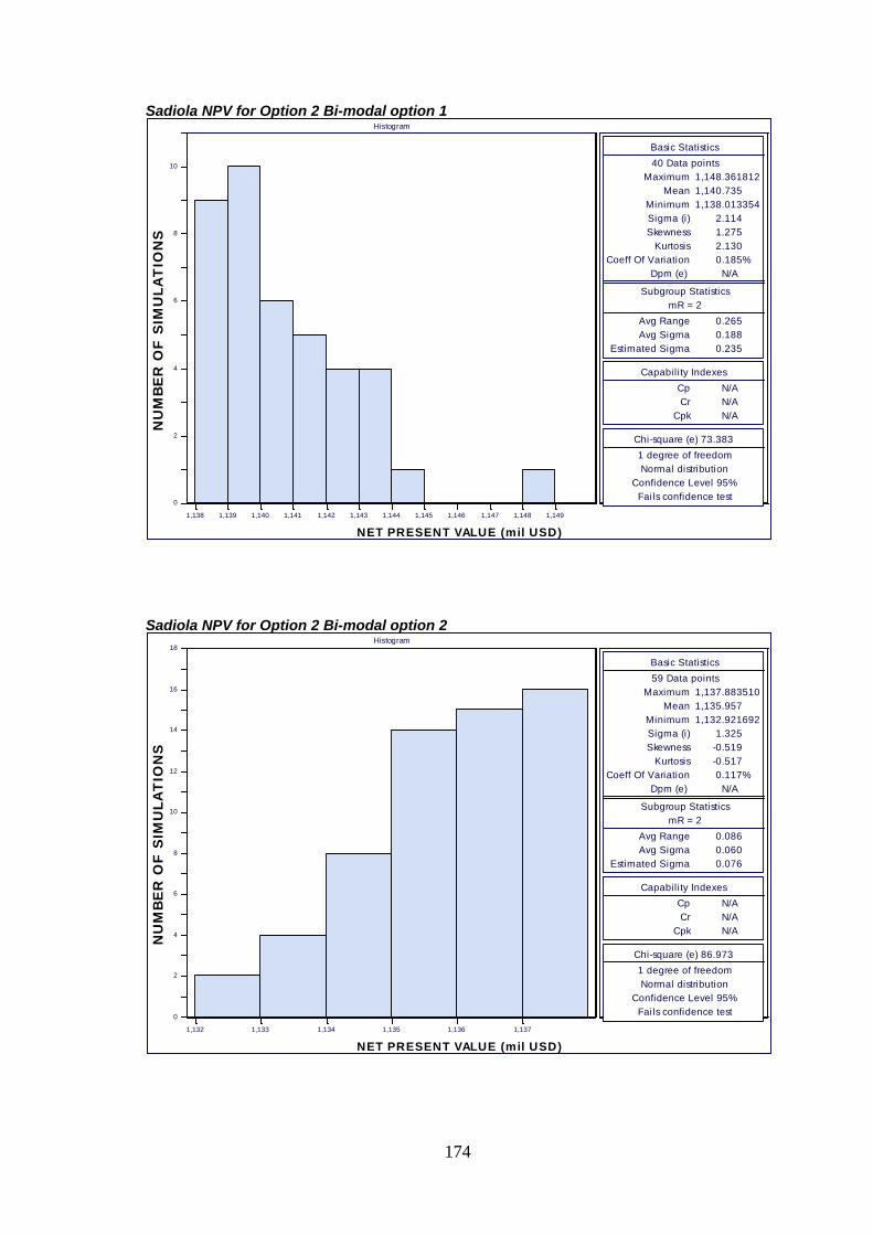
Sadiola NPV for Option 2 Bi-modal option 1 ...................................................... 174
Sadiola NPV for Option 2 Bi-modal option 2 ...................................................... 174
Sadiola NPV for Option 3 ................................................................................... 175
Sadiola gold price to cost per ounce for Option 1 ............................................... 175
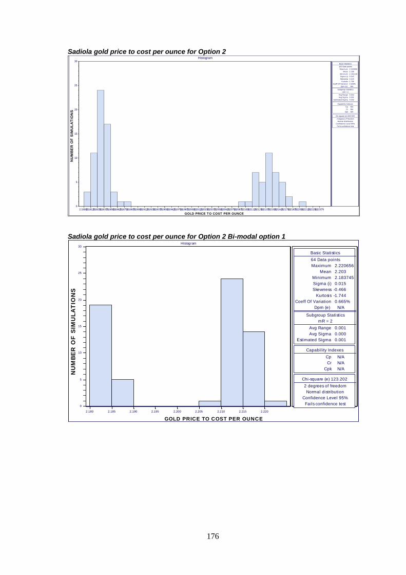
Sadiola gold price to cost per ounce for Option 2 ............................................... 176
Sadiola gold price to cost per ounce for Option 2 Bi-modal option 1 .................. 176
Page 12
xi
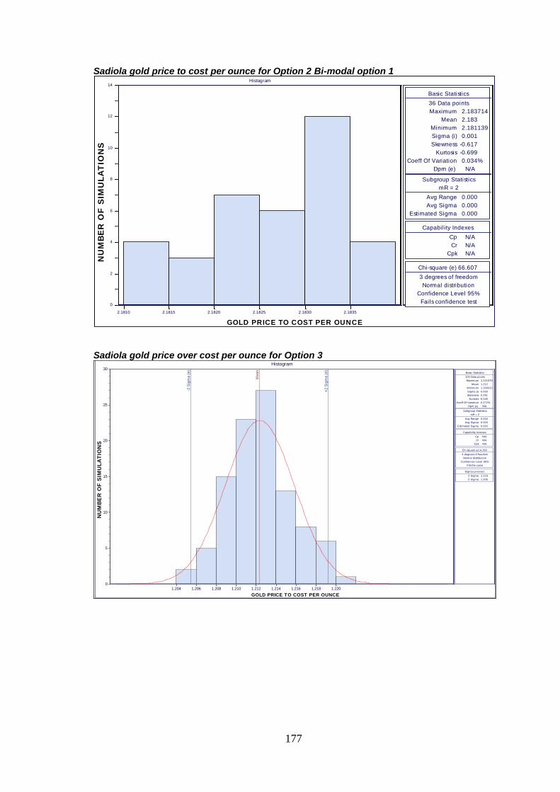
Sadiola gold price to cost per ounce for Option 2 Bi-modal option 1 .................. 177
Sadiola gold price over cost per ounce for Option 3 ........................................... 177
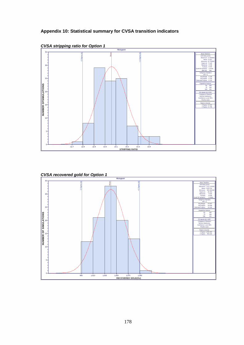
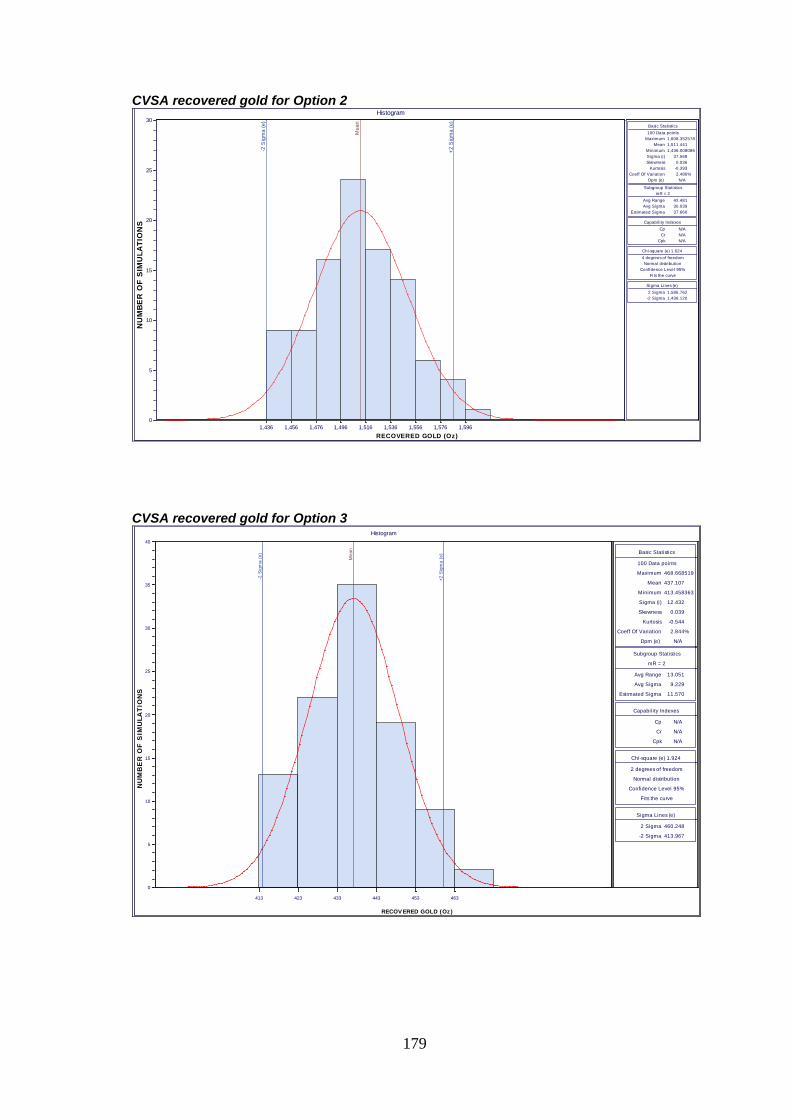
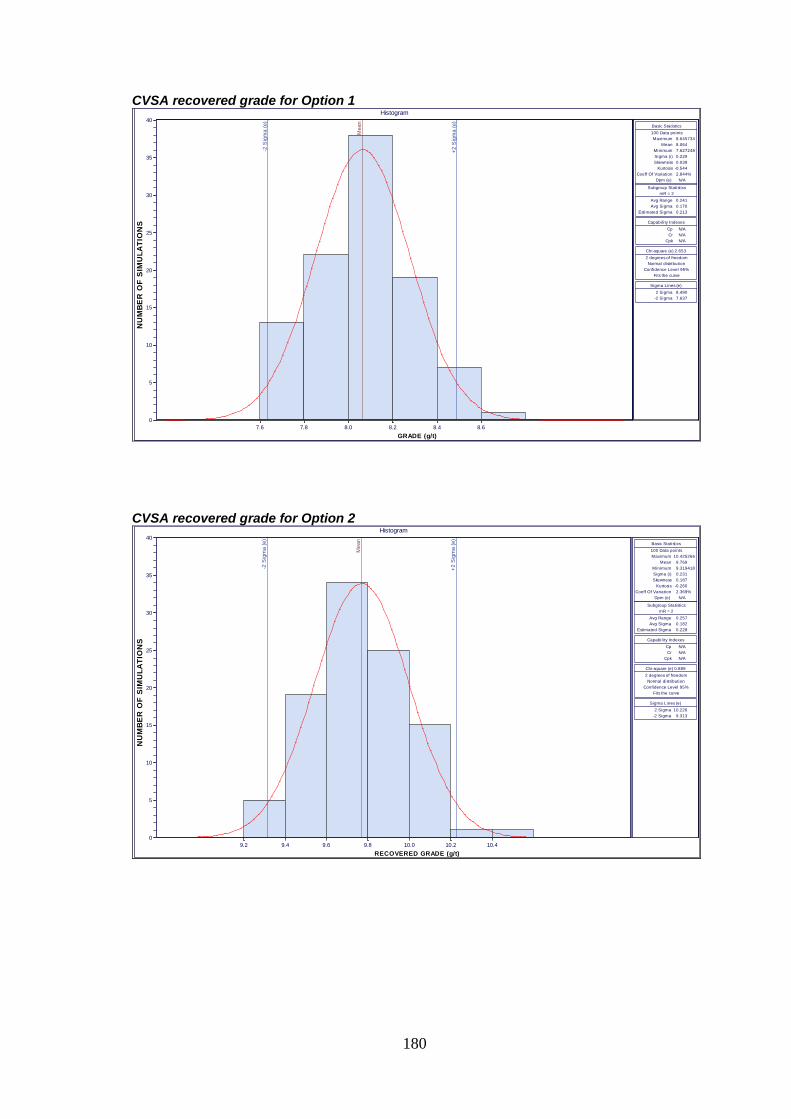
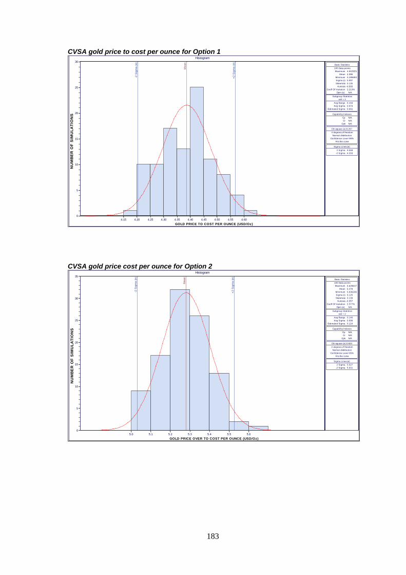
Appendix 10: Statistical summary for CVSA transition indicators ........................... 178
CVSA stripping ratio for Option 1 ....................................................................... 178
CVSA recovered gold for Option 1 ..................................................................... 178
CVSA recovered gold for Option 2 ..................................................................... 179
CVSA recovered gold for Option 3 ..................................................................... 179
CVSA recovered grade for Option 1 .................................................................. 180
CVSA recovered grade for Option 2 .................................................................. 180
CVSA recovered grade for Option 3 .................................................................. 181
CVSA NPV for Option 1 ..................................................................................... 181
CVSA NPV for Option 2 ..................................................................................... 182
CVSA NPV for Option 3 ..................................................................................... 182
CVSA gold price to cost per ounce for Option 1 ................................................. 183
CVSA gold price cost per ounce for Option 2 ..................................................... 183
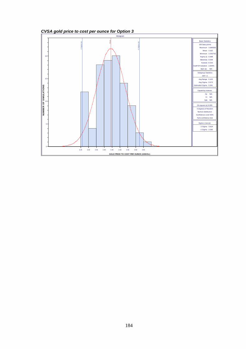
CVSA gold price to cost per ounce for Option 3 ................................................. 184
Appendix 11: Statistical summary for Geita transition indicators ............................ 185
Geita stripping ratio for Option 1 ........................................................................ 185
Geita stripping ratio for Option 1 Bi-modal option 1 ............................................ 185
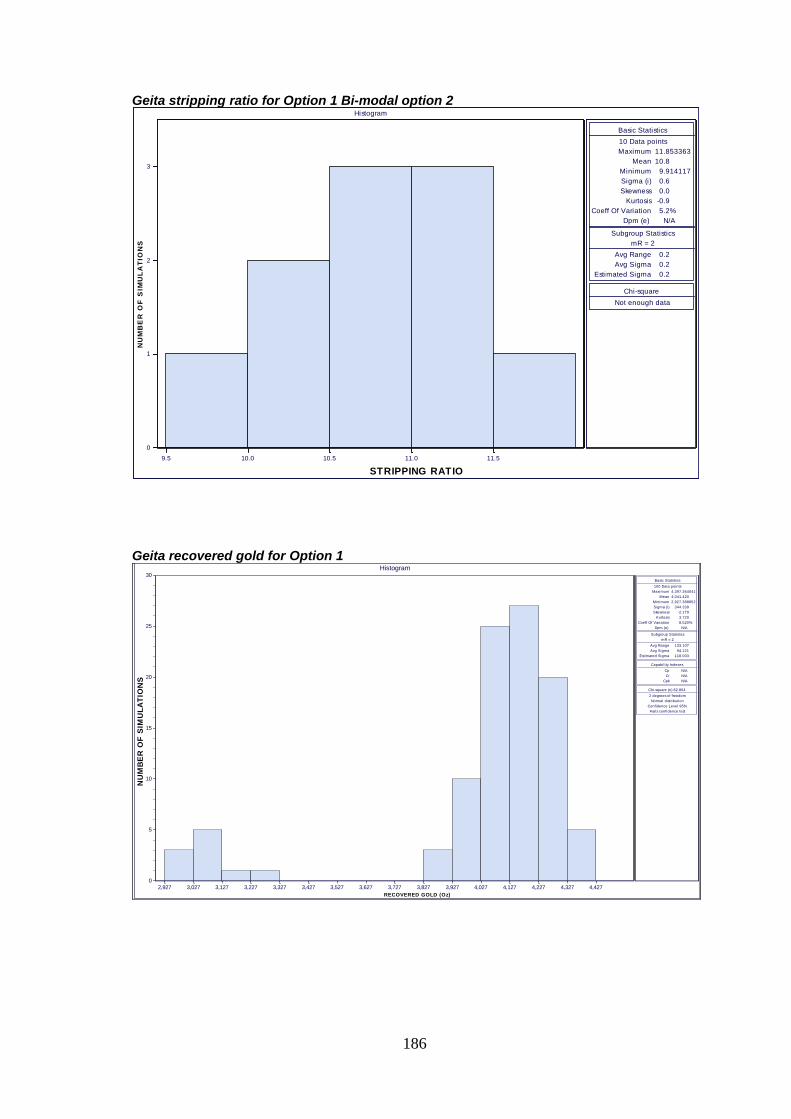
Geita stripping ratio for Option 1 Bi-modal option 2 ............................................ 186
Geita recovered gold for Option 1 ...................................................................... 186
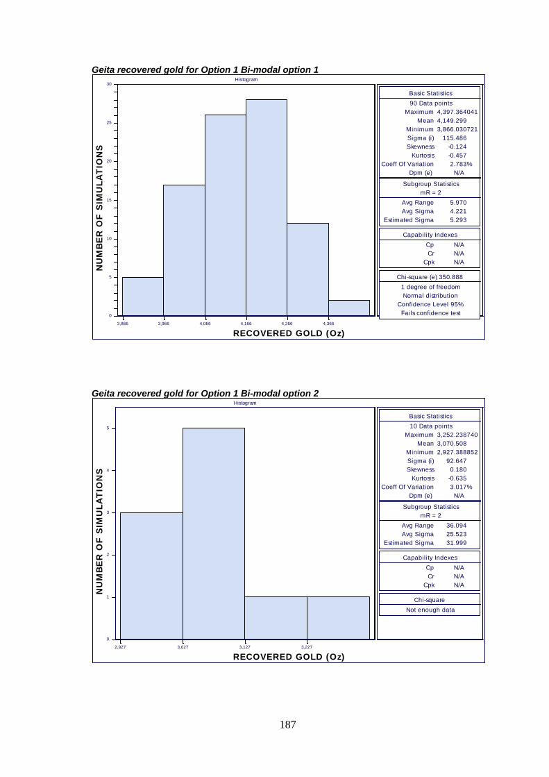
Geita recovered gold for Option 1 Bi-modal option 1 ......................................... 187
Geita recovered gold for Option 1 Bi-modal option 2 ......................................... 187
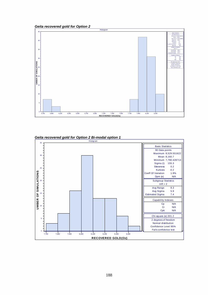
Geita recovered gold for Option 2 ...................................................................... 188
Geita recovered gold for Option 2 Bi-modal option 1 ......................................... 188
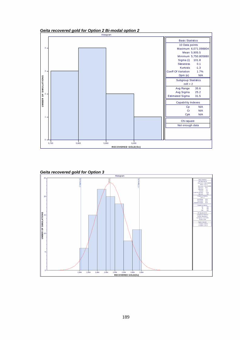
Geita recovered gold for Option 2 Bi-modal option 2 ......................................... 189
Geita recovered gold for Option 3 ...................................................................... 189
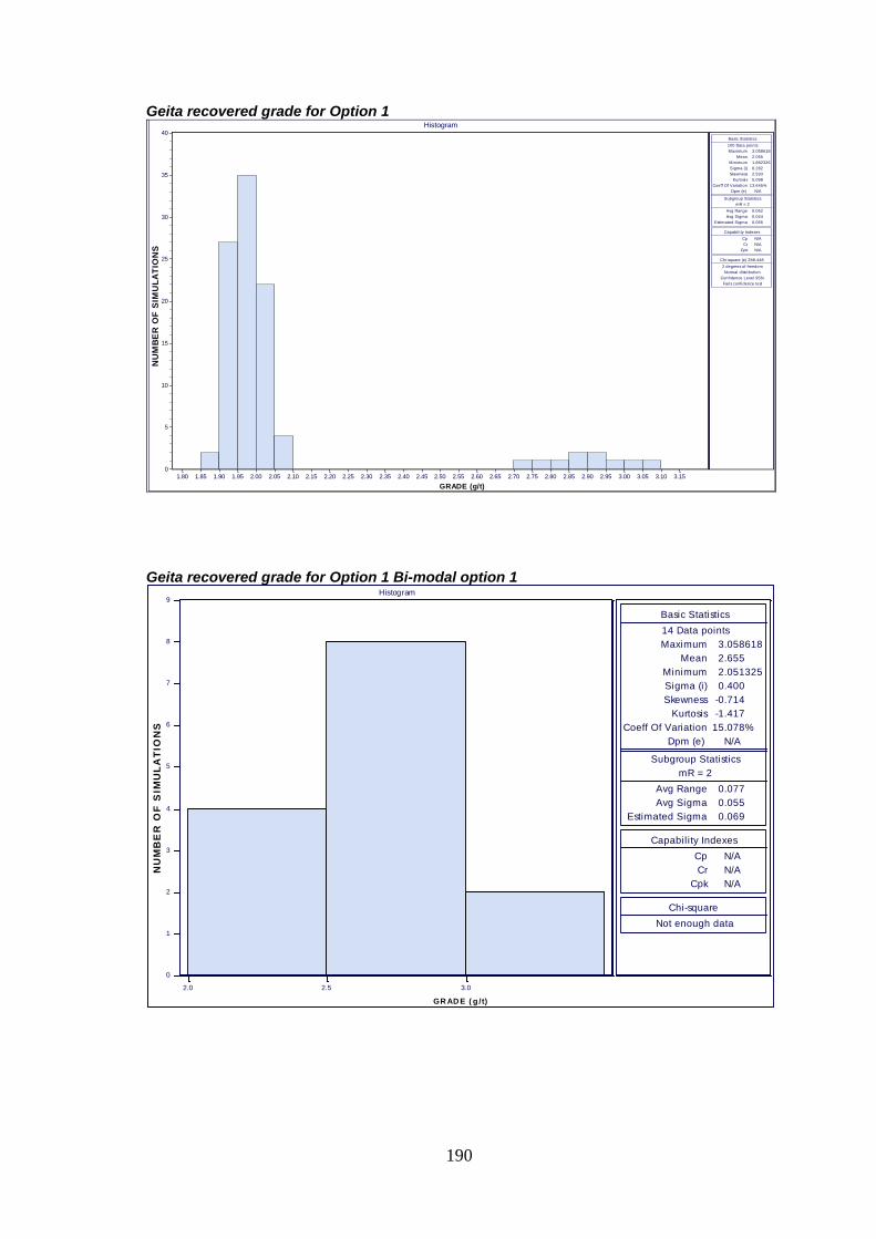
Geita recovered grade for Option 1.................................................................... 190
Geita recovered grade for Option 1 Bi-modal option 1 ....................................... 190
Page 13
xii
Geita recovered grade for Option 1 Bi-modal option 2 ....................................... 191
Geita recovered grade for Option 2.................................................................... 191
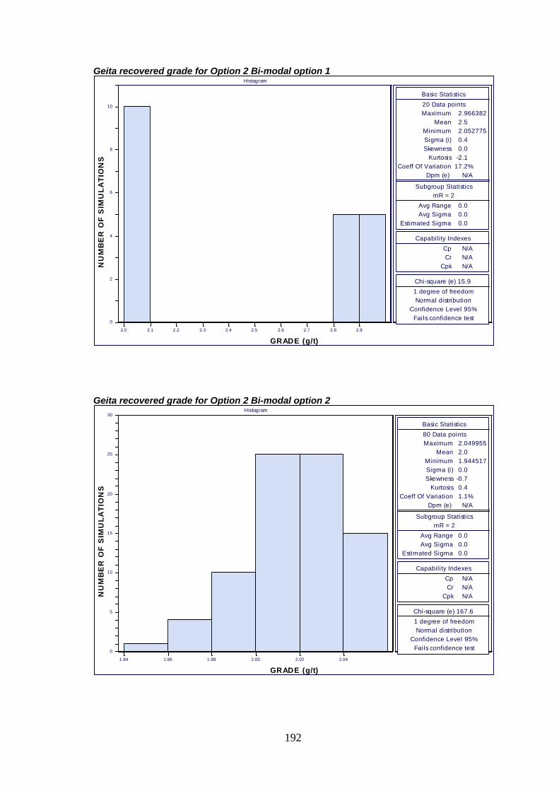
Geita recovered grade for Option 2 Bi-modal option 1 ....................................... 192
Geita recovered grade for Option 2 Bi-modal option 2 ....................................... 192
Geita recovered grade for Option 3.................................................................... 193
Geita NPV for Option 1 ...................................................................................... 193
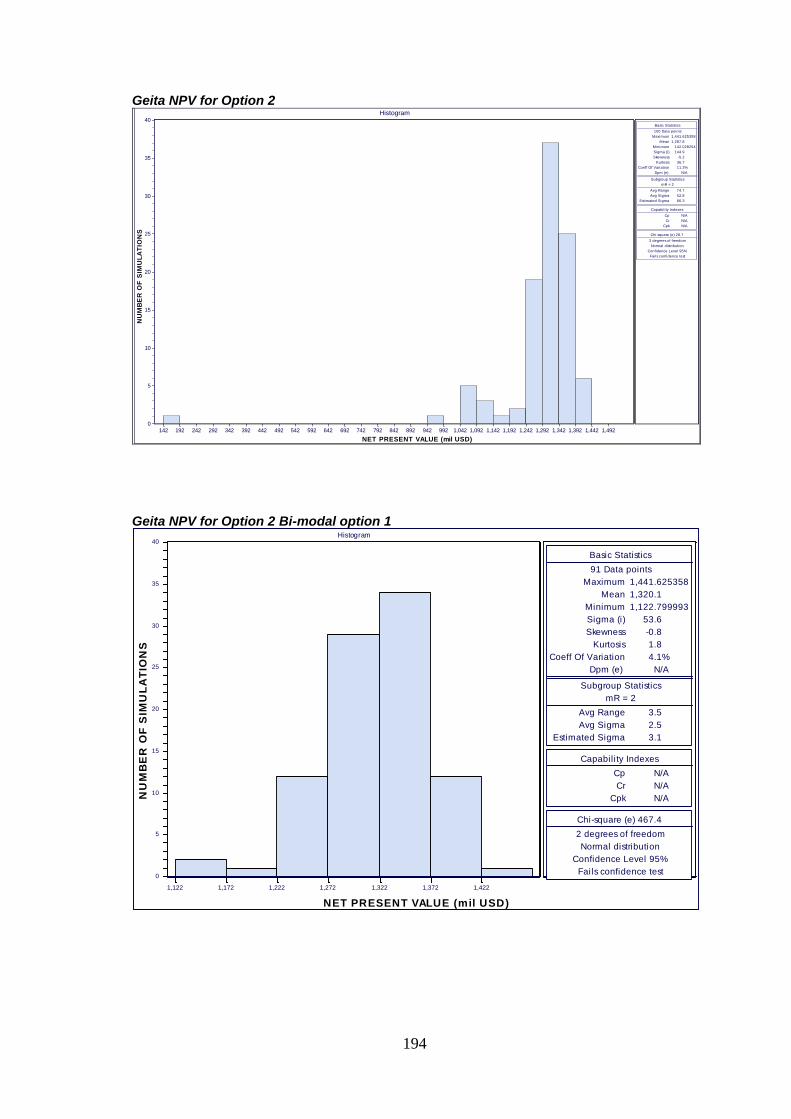
Geita NPV for Option 2 ...................................................................................... 194
Geita NPV for Option 2 Bi-modal option 1 .......................................................... 194
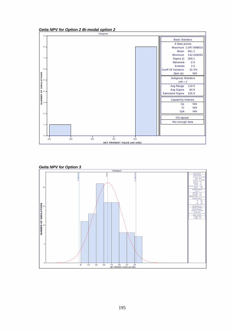
Geita NPV for Option 2 Bi-modal option 2 .......................................................... 195
Geita NPV for Option 3 ...................................................................................... 195
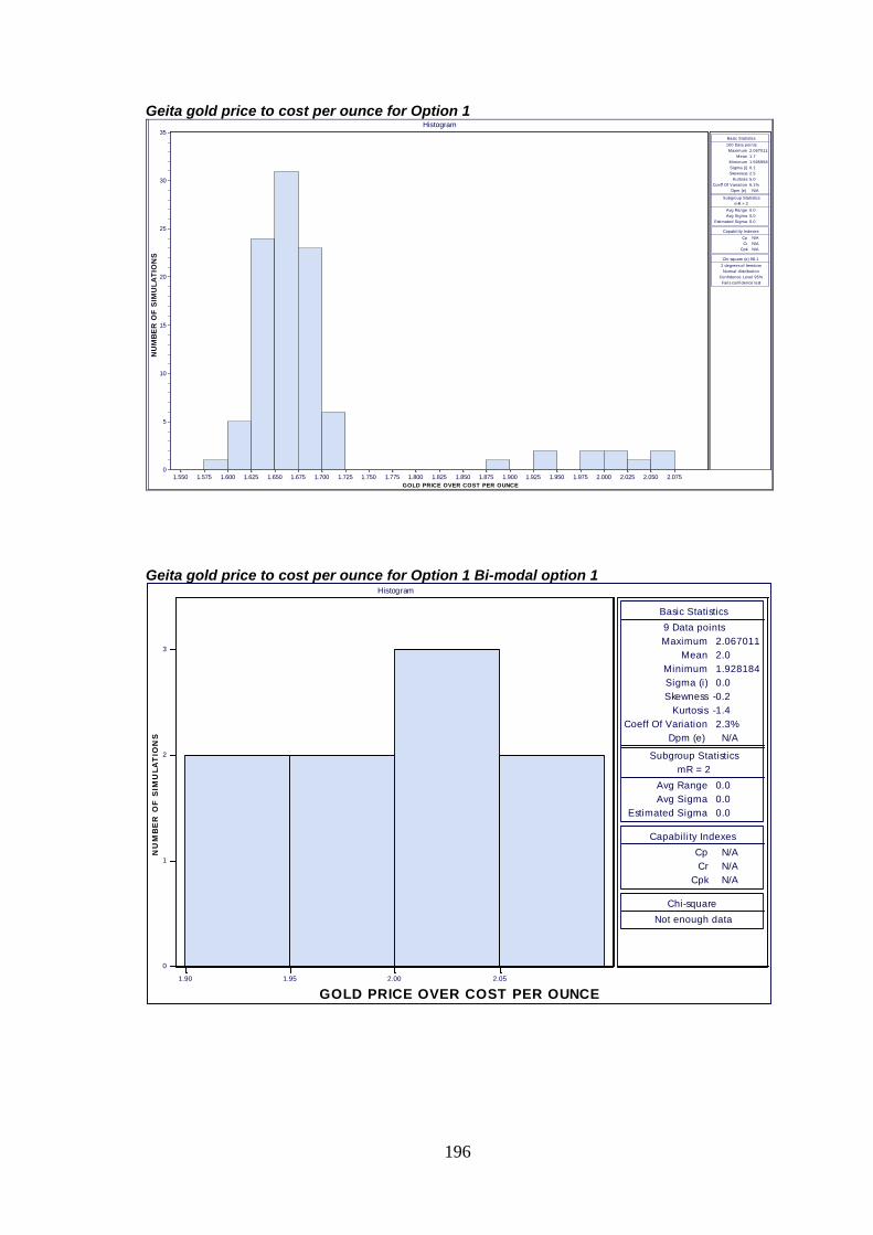
Geita gold price to cost per ounce for Option 1 .................................................. 196
Geita gold price to cost per ounce for Option 1 Bi-modal option 1 ..................... 196
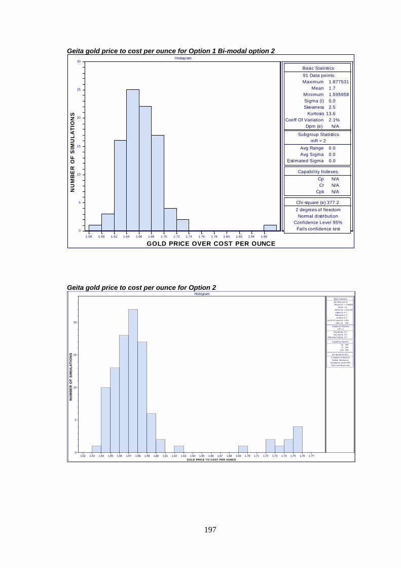
Geita gold price to cost per ounce for Option 1 Bi-modal option 2 ..................... 197
Geita gold price to cost per ounce for Option 2 .................................................. 197
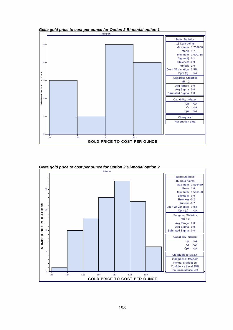
Geita gold price to cost per ounce for Option 2 Bi-modal option 1 ..................... 198
Geita gold price to cost per ounce for Option 2 Bi-modal option 2 ..................... 198
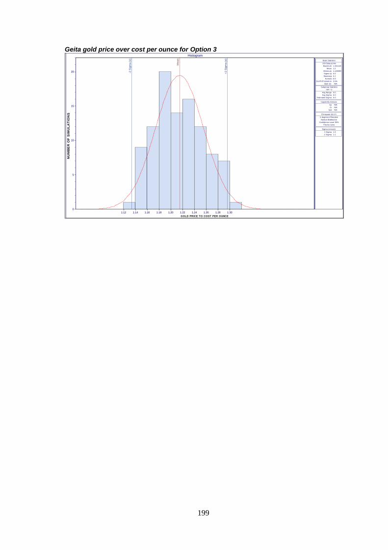
Geita gold price over cost per ounce for Option 3 .............................................. 199
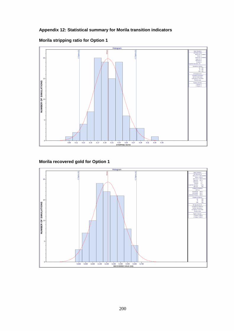
Appendix 12: Statistical summary for Morila transition indicators ........................... 200
Morila stripping ratio for Option 1 ....................................................................... 200
Morila recovered gold for Option 1 ..................................................................... 200
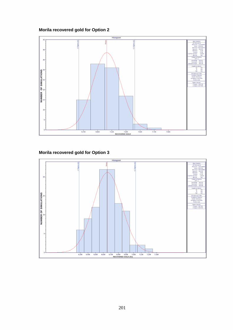
Morila recovered gold for Option 2 ..................................................................... 201
Morila recovered gold for Option 3 ..................................................................... 201
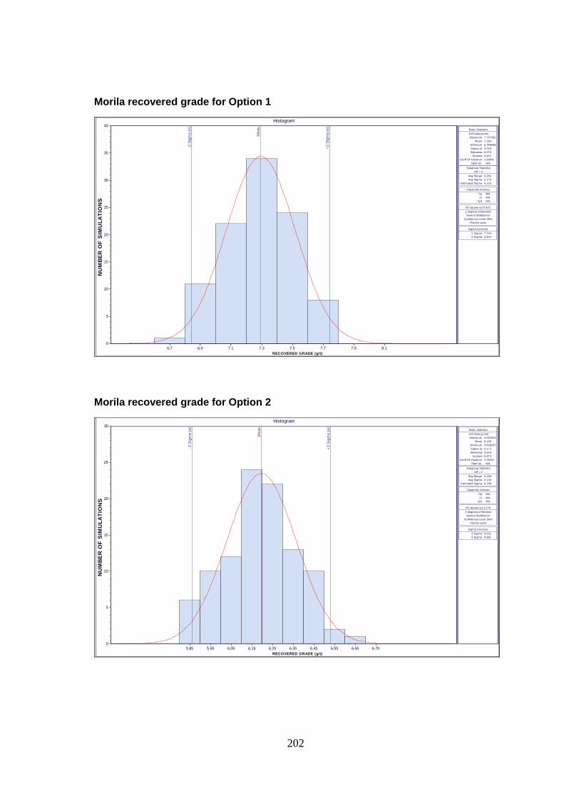
Morila recovered grade for Option 1 .................................................................. 202
Morila recovered grade for Option 2 .................................................................. 202
Morila recovered grade for Option 3 .................................................................. 203
Morila NPV for Option 1 ..................................................................................... 203
Morila NPV for Option 2 ..................................................................................... 204
Morila NPV for Option 3 ..................................................................................... 204
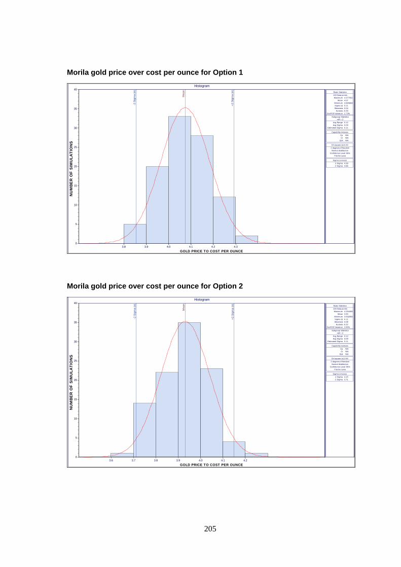
Morila gold price over cost per ounce for Option 1 ............................................. 205
Page 14
xiii
Morila gold price over cost per ounce for Option 2 ............................................. 205
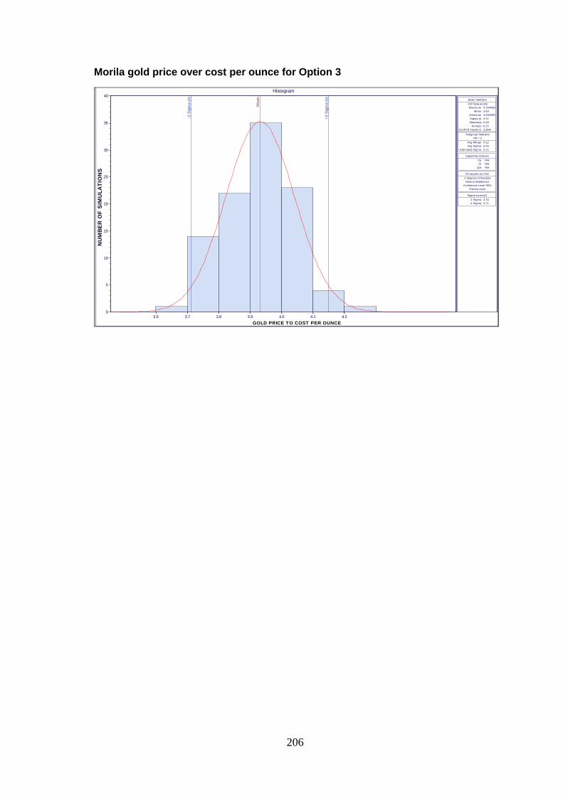
Morila gold price over cost per ounce for Option 3 ............................................. 206
Page 15
xiv
LIST OF FIGURES
FIGURE PAGE
Figure 1-1: 3D view of open pit to underground transition (Courtesy: AngloGold Ashanti
Limited) ........................................................................................................................ 1
Figure 1-2: Layout of thesis structure ..........................................................................10
Figure 2-1: Transition depth [Bakhtavar et al (2008)] ...................................................15
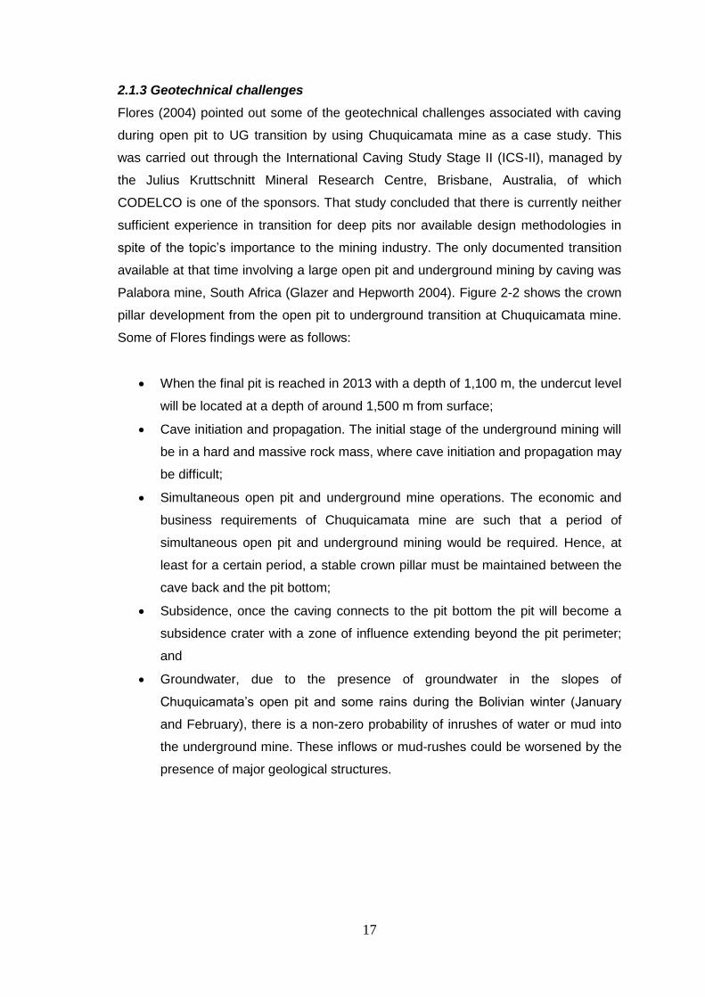
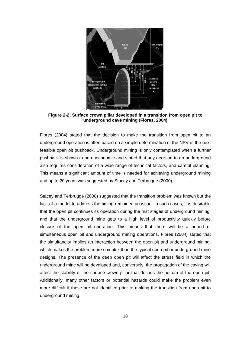
Figure 2-2: Surface crown pillar developed in a transition from open pit to underground
cave mining (Flores, 2004) ..........................................................................................18
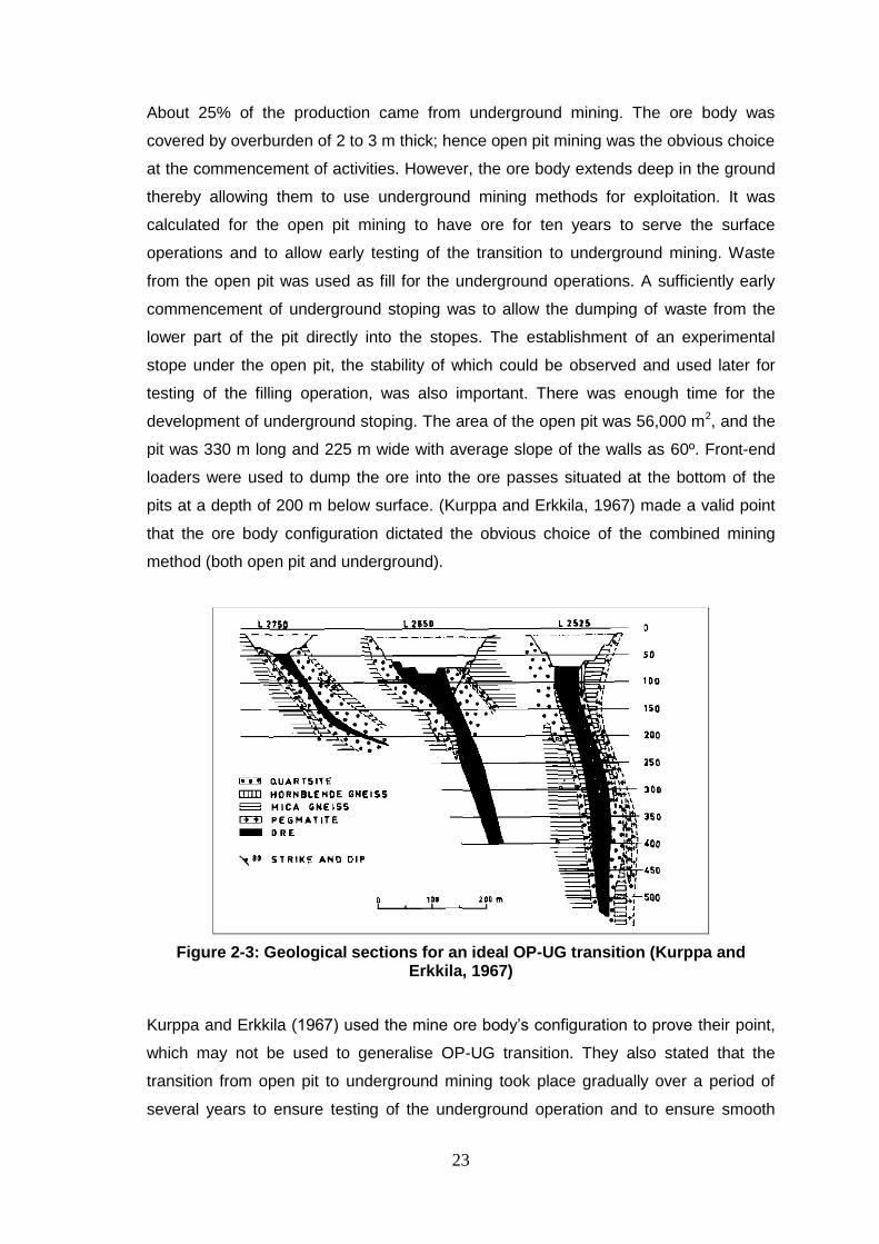
Figure 2-3: Geological sections for an ideal OP-UG transition (Kurppa and Erkkila,
1967) ...........................................................................................................................23
Figure 2-4: OP – UG transition framework ...................................................................26
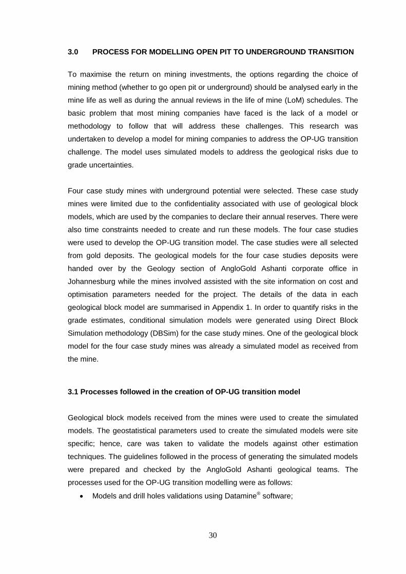
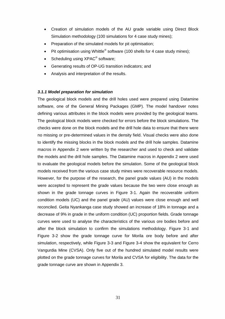
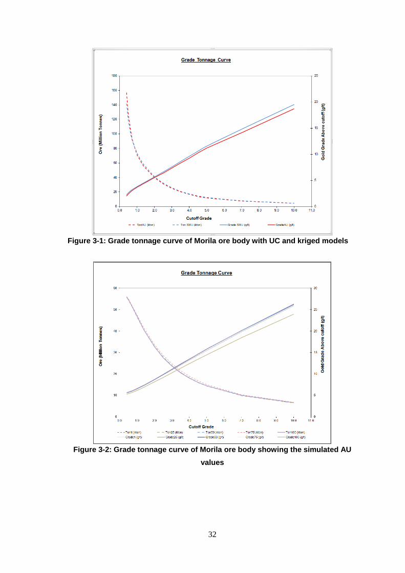
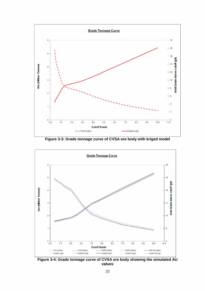
Figure 3-1: Grade tonnage curve of Morila ore body with UC and kriged models ........32
Figure 3-2: Grade tonnage curve of Morila ore body showing the simulated AU values
....................................................................................................................................32
Figure 3-3: Grade tonnage curve of CVSA ore body with kriged model .......................33
Figure 3-4: Grade tonnage curve of CVSA ore body showing the simulated AU values
....................................................................................................................................33
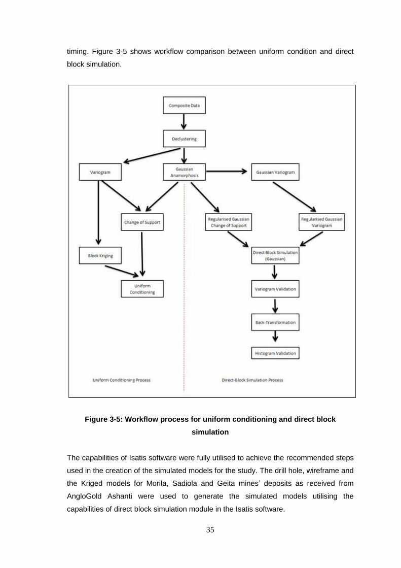
Figure 3-5: Workflow process for uniform conditioning and direct block simulation ......35
Figure 3-6: Gaussian point variogram window .............................................................37
Figure 3-7: Point variogram fitting window ...................................................................37
Figure 3-8 : Variogram validation window ....................................................................38
Figure 3-9: Workflow for creation of simulated models with the direct block simulation
method (Source: Geovariances) ..................................................................................38
Figure 3-10 : Flowchart of model preparation macros ..................................................40
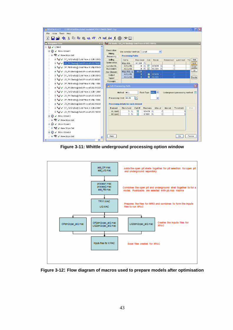
Figure 3-11: Whittle underground processing option window .......................................43
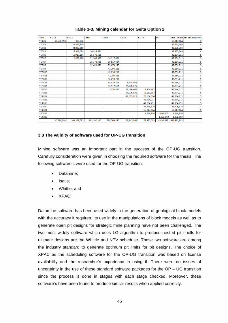
Figure 3-12: Flow diagram of macros used to prepare models after optimisation ........43
Figure 4-1: Map showing the location of Geita Gold Mine (Courtesy: GGM) ................50
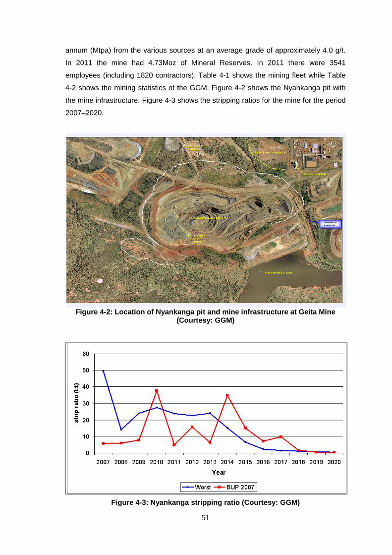
Figure 4-2: Location of Nyankanga pit and mine infrastructure at Geita Mine (Courtesy:
GGM) ..........................................................................................................................51
Figure 4-3: Nyankanga stripping ratio (Courtesy: GGM) ..............................................51
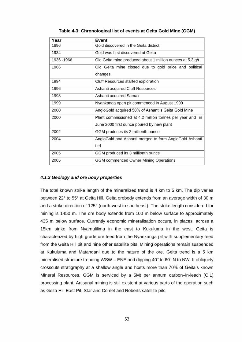
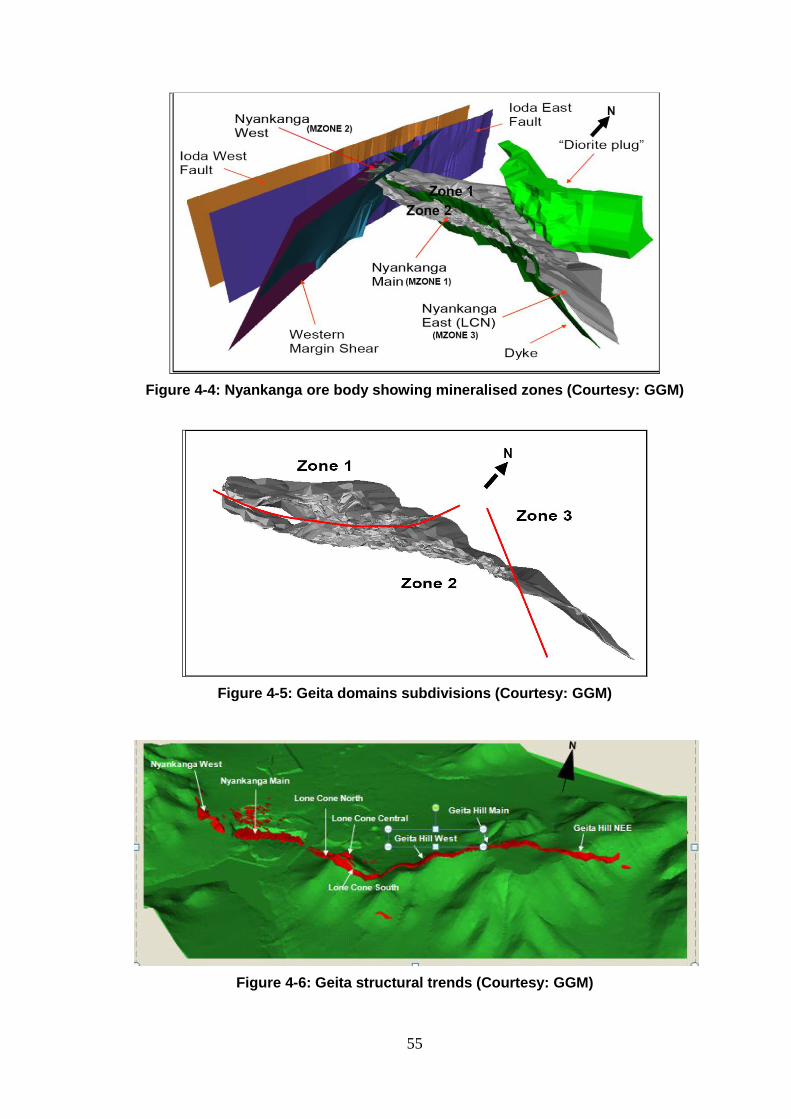
Figure 4-4: Nyankanga ore body showing mineralised zones (Courtesy: GGM) ..........55
Figure 4-5: Geita domains subdivisions (Courtesy: GGM) ...........................................55
Figure 4-6: Geita structural trends (Courtesy: GGM) ...................................................55
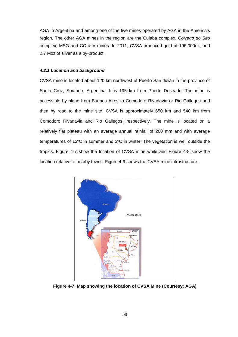
Figure 4-7: Map showing the location of CVSA Mine (Courtesy: AGA) ........................58
Figure 4-8: Location of CVSA Mine relative to nearby towns (www:argentina.gov.ar) ..59
Page 16
xv
Figure 4-9: Site plan of CVSA (Courtesy: AGA) ...........................................................59
Figure 4-10: Stripping ratio variation for CVSA ............................................................60
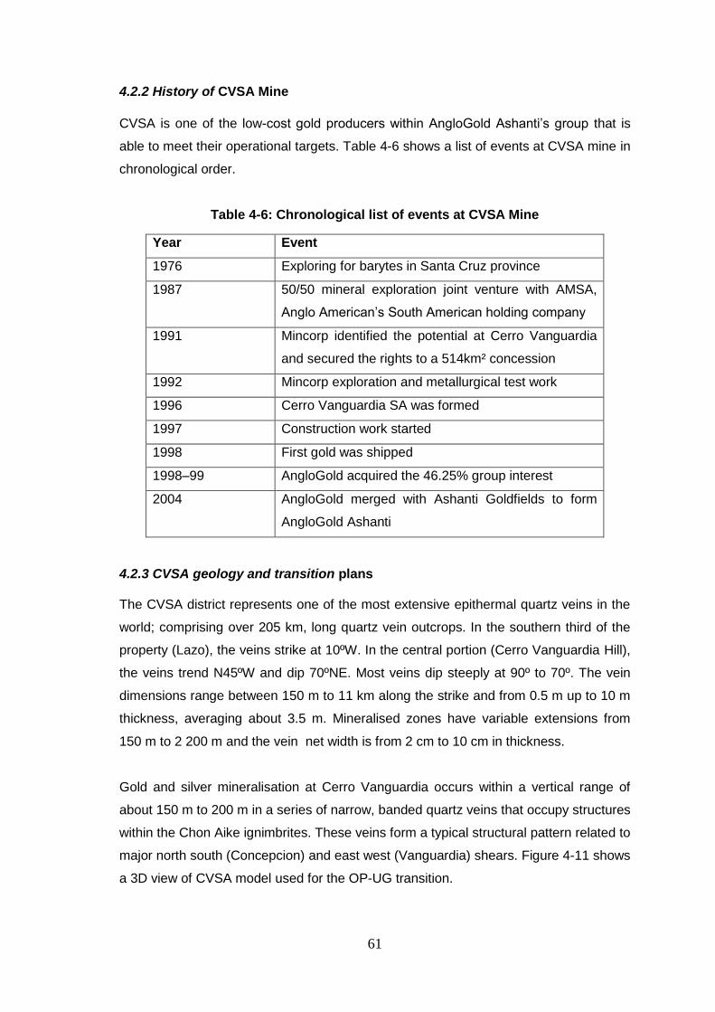
Figure 4-11: 3D view of CVSA model for the project (Courtesy: CVSA Mine) ..............62
Figure 4-12: Map showing location of Sadiola Mine (Courtesy: AGA) ..........................63
Figure 4-13: W-E section showing the various material types (Courtesy: AGA) ...........65
Figure 4-14: Map showing the location of Morila mine (Courtesy: AGA) ......................67
Figure 4-15: Section through Morila ore body (Courtesy: Morila Gold Mine) ................69
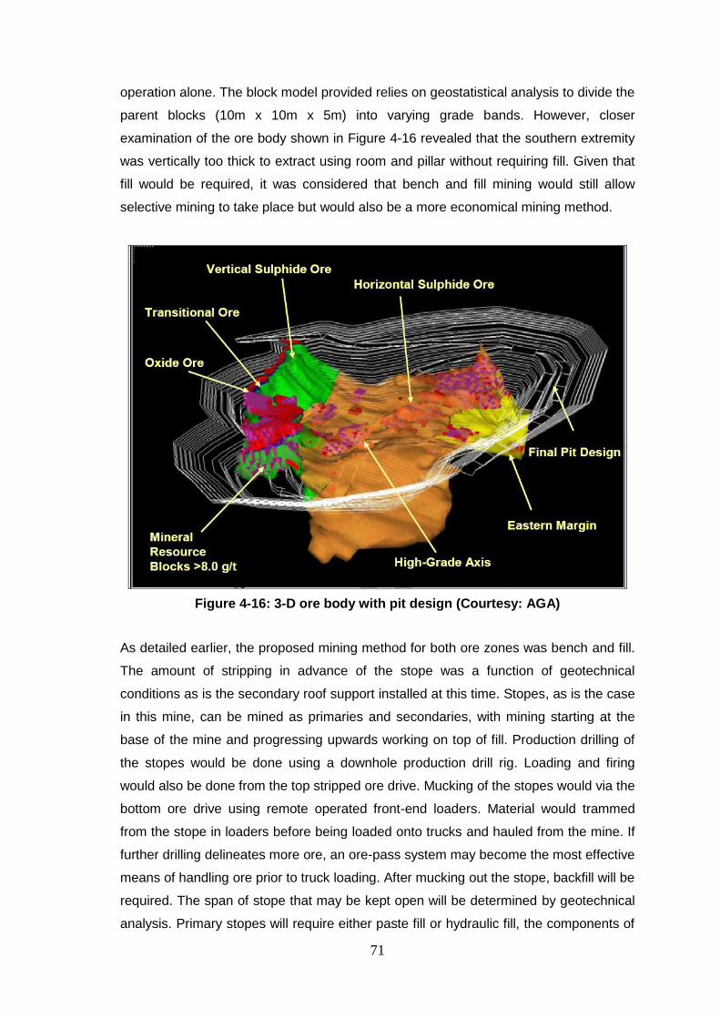
Figure 4-16: 3-D ore body with pit design (Courtesy: AGA) .........................................71
Figure 5-1: Location of Sunrise Dam Gold Mine (Courtesy: AGA) ...............................73
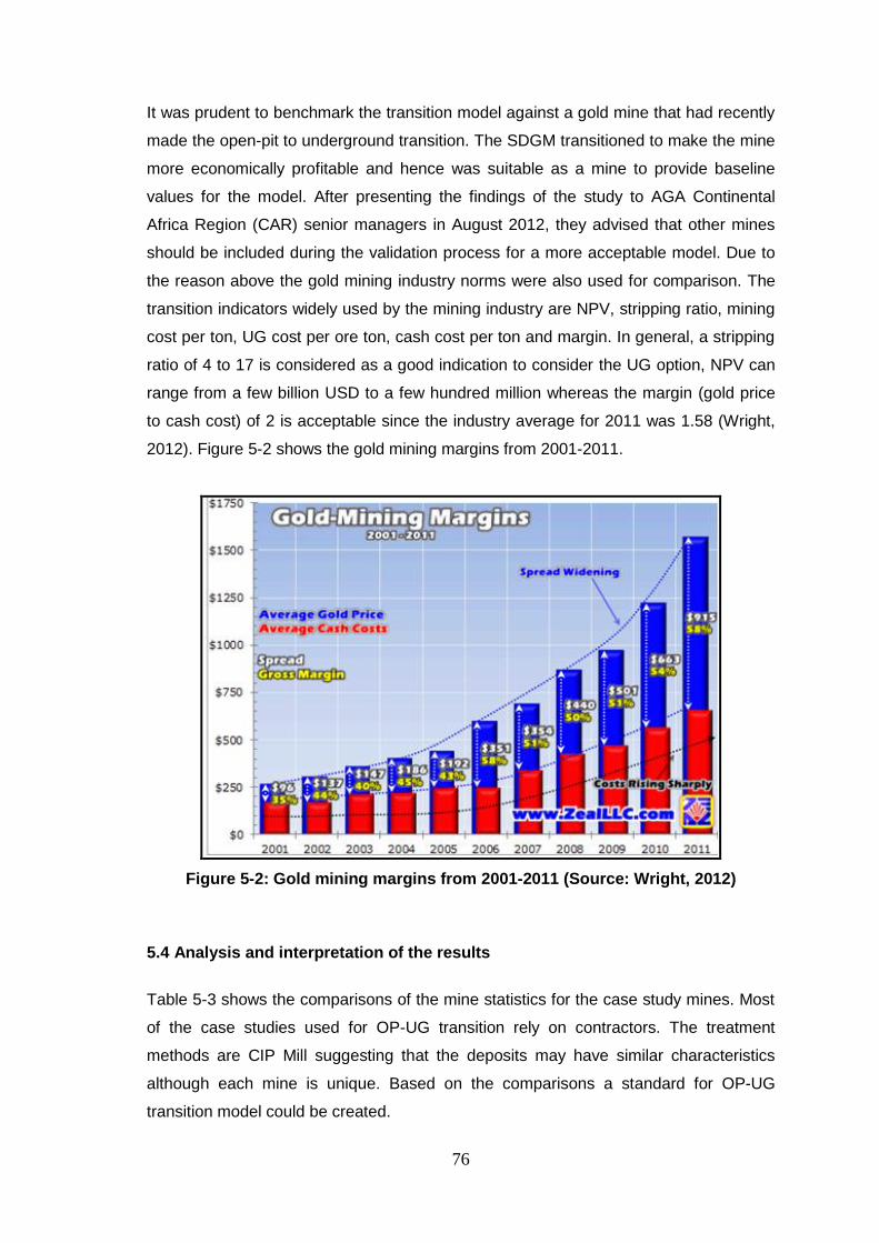
Figure 5-2: Gold mining margins from 2001-2011 (Source: Wright, 2012) ...................76
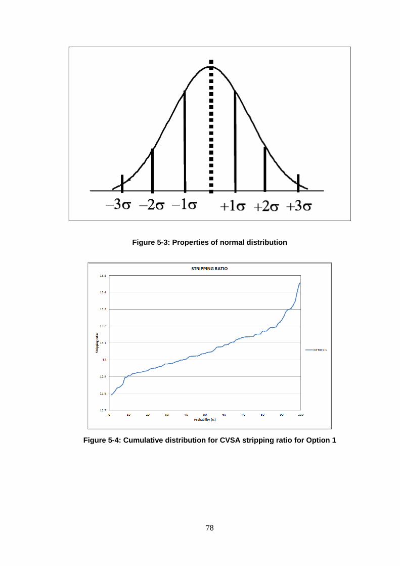
Figure 5-3: Properties of normal distribution ................................................................78
Figure 5-4: Cumulative distribution for CVSA stripping ratio for Option 1 .....................78
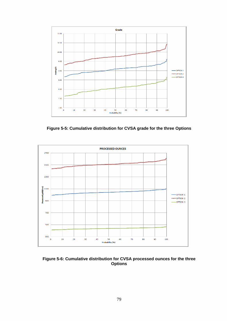
Figure 5-5: Cumulative distribution for CVSA grade for the three Options ...................79
Figure 5-6: Cumulative distribution for CVSA processed ounces for the three Options 79
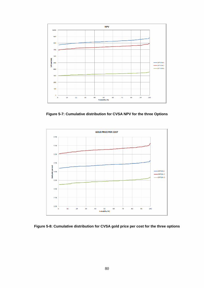
Figure 5-7: Cumulative distribution for CVSA NPV for the three Options .....................80
Figure 5-8: Cumulative distribution for CVSA gold price per cost for the three options 80
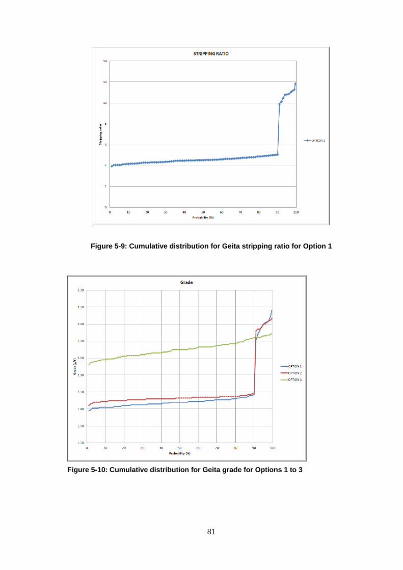
Figure 5-9: Cumulative distribution for Geita stripping ratio for Option 1 ......................81
Figure 5-10: Cumulative distribution for Geita grade for Options 1 to 3........................81
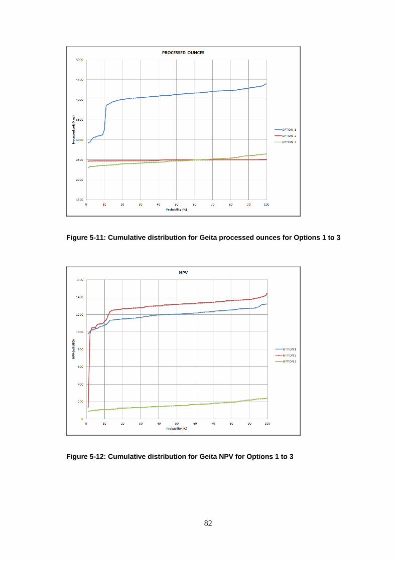
Figure 5-11: Cumulative distribution for Geita processed ounces for Options 1 to 3 ....82
Figure 5-12: Cumulative distribution for Geita NPV for Options 1 to 3 .........................82
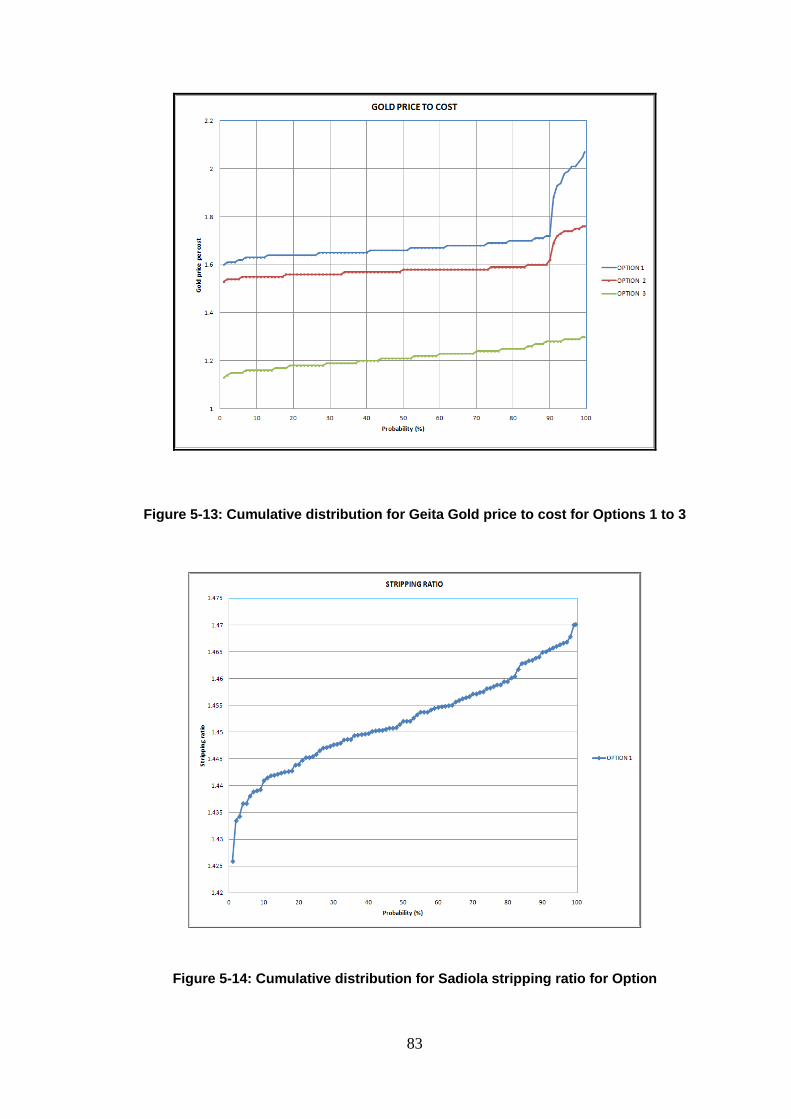
Figure 5-13: Cumulative distribution for Geita Gold price to cost for Options 1 to 3 .....83
Figure 5-14: Cumulative distribution for Sadiola stripping ratio for Option ....................83
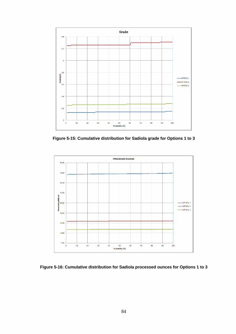
Figure 5-15: Cumulative distribution for Sadiola grade for Options 1 to 3 ....................84
Figure 5-16: Cumulative distribution for Sadiola processed ounces for Options 1 to 3 .84
Figure 5-17: Cumulative distribution for Sadiola NPV for Options 1 to 3 ......................85
Figure 5-18: Cumulative distribution for Sadiola gold price to cost for Options 1 to 3...85
Figure 5-19: Cumulative distribution for Morila stripping ratio for Option 1 ...................86
Figure 5-20: Cumulative distribution for Morila grade for Options 1 to 3 ......................86
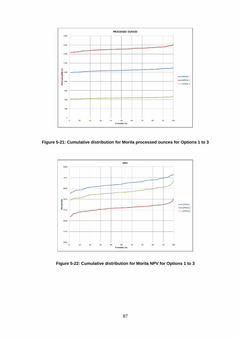
Figure 5-21: Cumulative distribution for Morila processed ounces for Options 1 to 3 ...87
Figure 5-22: Cumulative distribution for Morila NPV for Options 1 to 3 ........................87
Figure 5-23: Cumulative distribution for Morila gold price to cost for Options 1 to 3 .....88
Figure 5-24: Sectional view of CVSA showing pit outlines ...........................................89
Figure 5-25: Sadiola recovered gold for Option 2 with Bi-modal distribution ................89
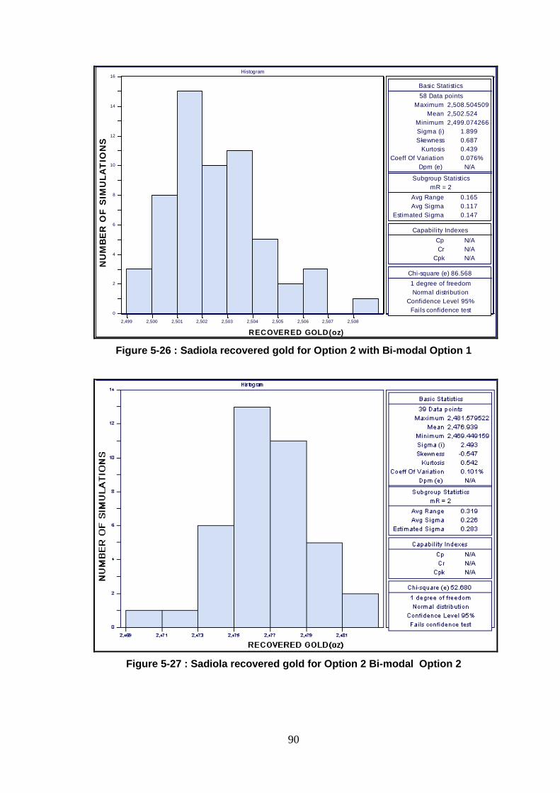
Figure 5-26 : Sadiola recovered gold for Option 2 with Bi-modal Option 1 ...................90
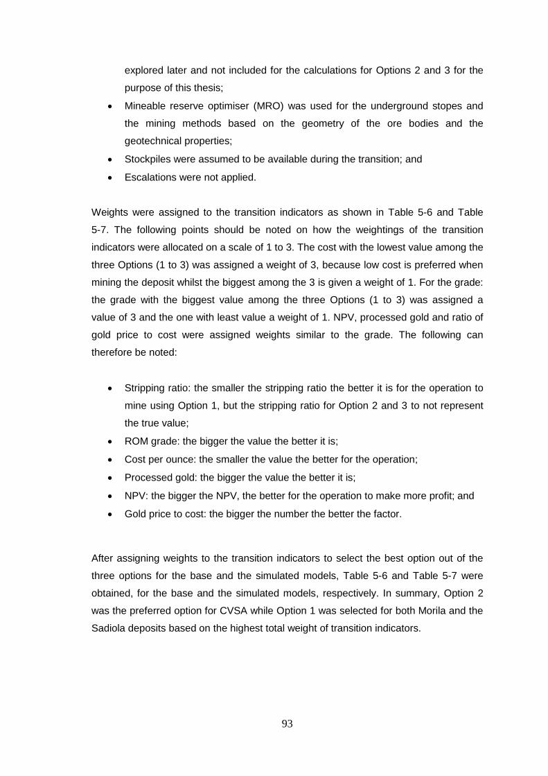
Figure 5-27 : Sadiola recovered gold for Option 2 Bi-modal Option 2 .........................90
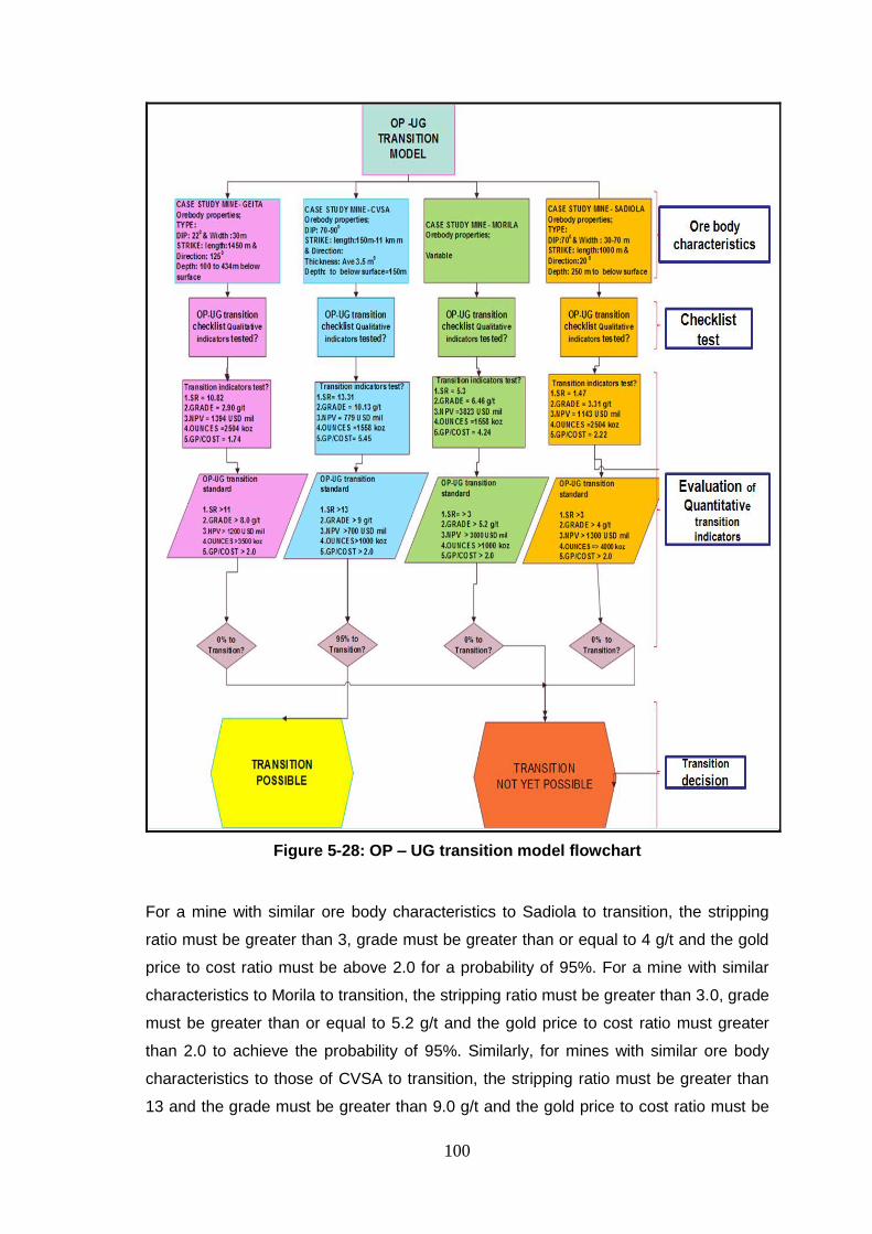
Figure 5-28: OP – UG transition model flowchart ...................................................... 100
Page 17
xvi
LIST OF TABLES
TABLE ................................................................................................................ PAGE
Table 1-1: Status of some open pit to underground transition mines ............................ 6
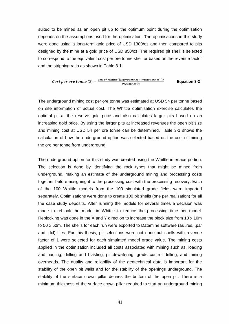
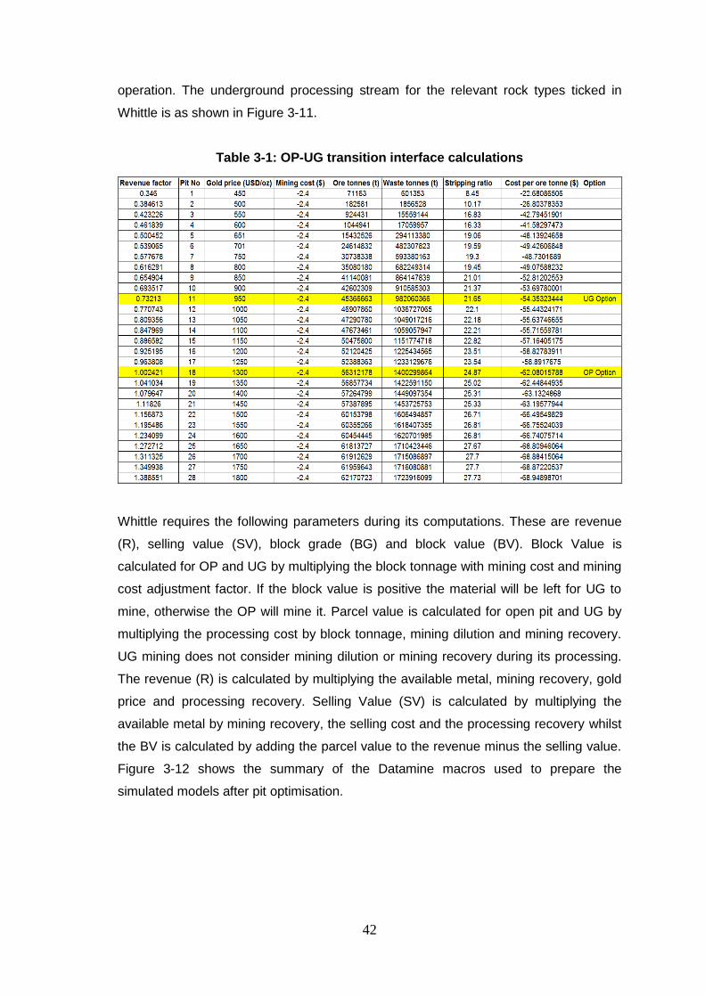
Table 3-1: OP-UG transition interface calculations ......................................................42
Table 3-2: Mining calendar for Geita Option 1 .............................................................45
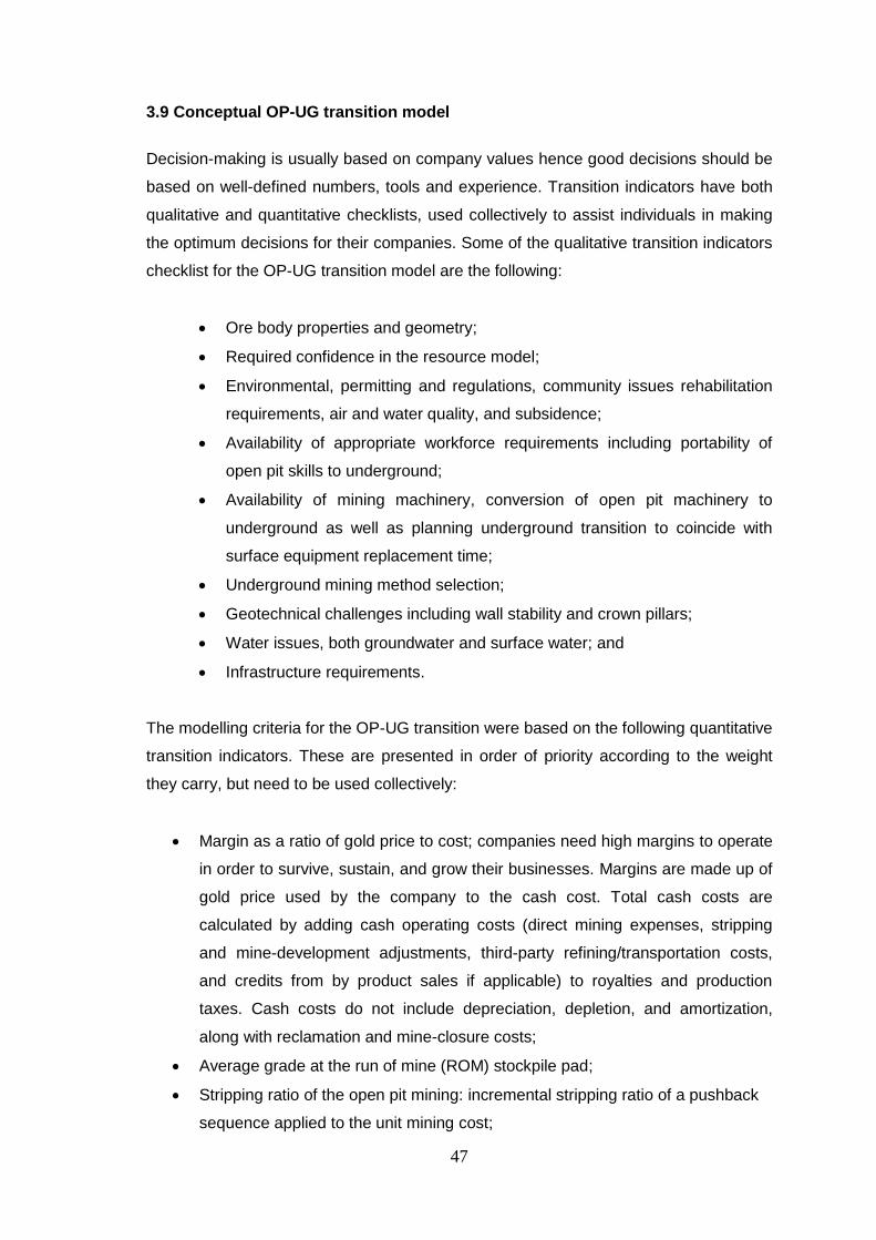
Table 3-3: Mining calendar for Geita Option 2 .............................................................46
Table 4-1: Open pit mining fleet for Geita Mine ...........................................................52
Table 4-2: Geita mining statistics .................................................................................52
Table 4-3: Chronological list of events at Geita Gold Mine (GGM) ...............................53
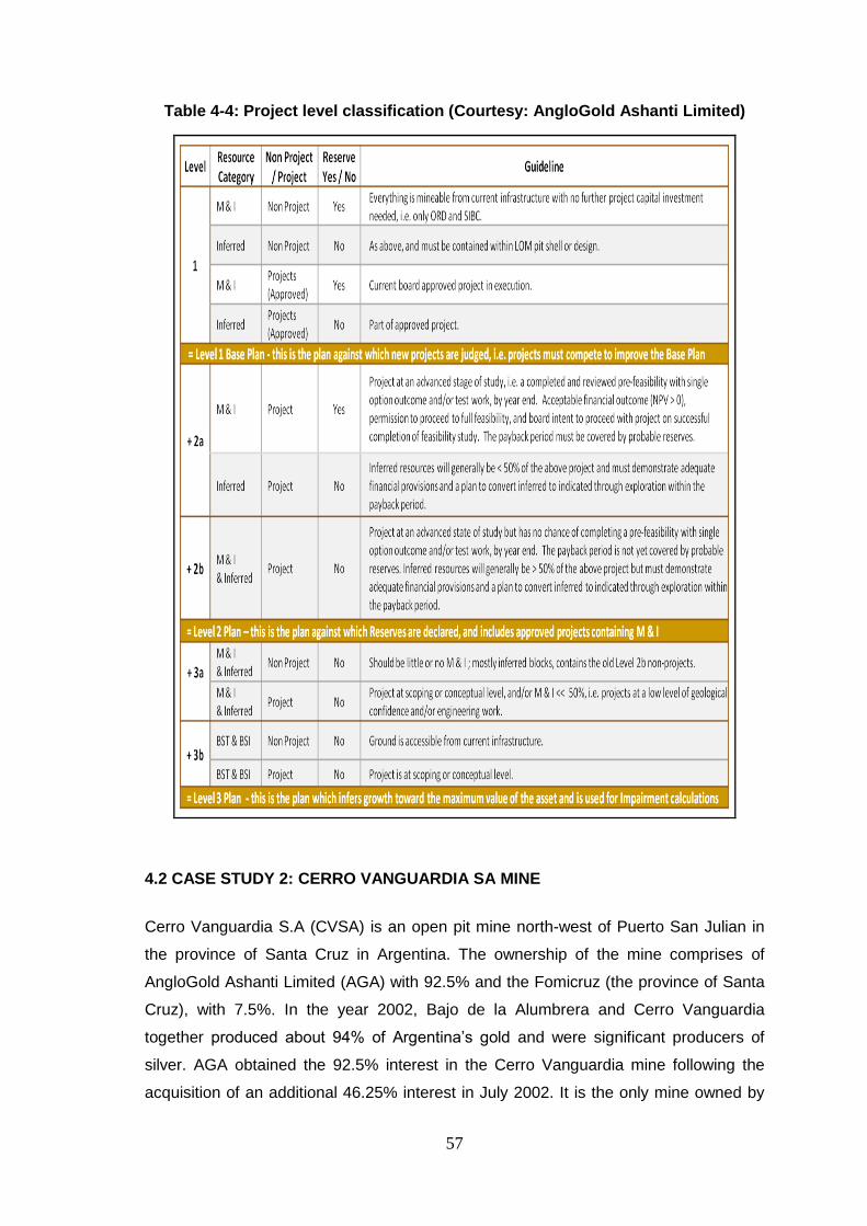
Table 4-4: Project level classification (Courtesy: AngloGold Ashanti Limited) ..............57
Table 4-5: CVSA mining fleet ......................................................................................60
Table 4-6: Chronological list of events at CVSA Mine ..................................................61
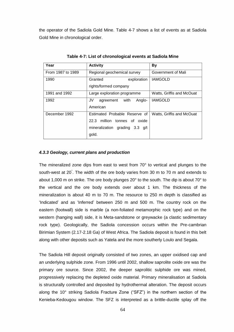
Table 4-7: List of chronological events at Sadiola Mine ...............................................64
Table 4-8: Sadiola mining fleet ....................................................................................66
Table 4-9: List of events at Morila Gold Mine...............................................................68
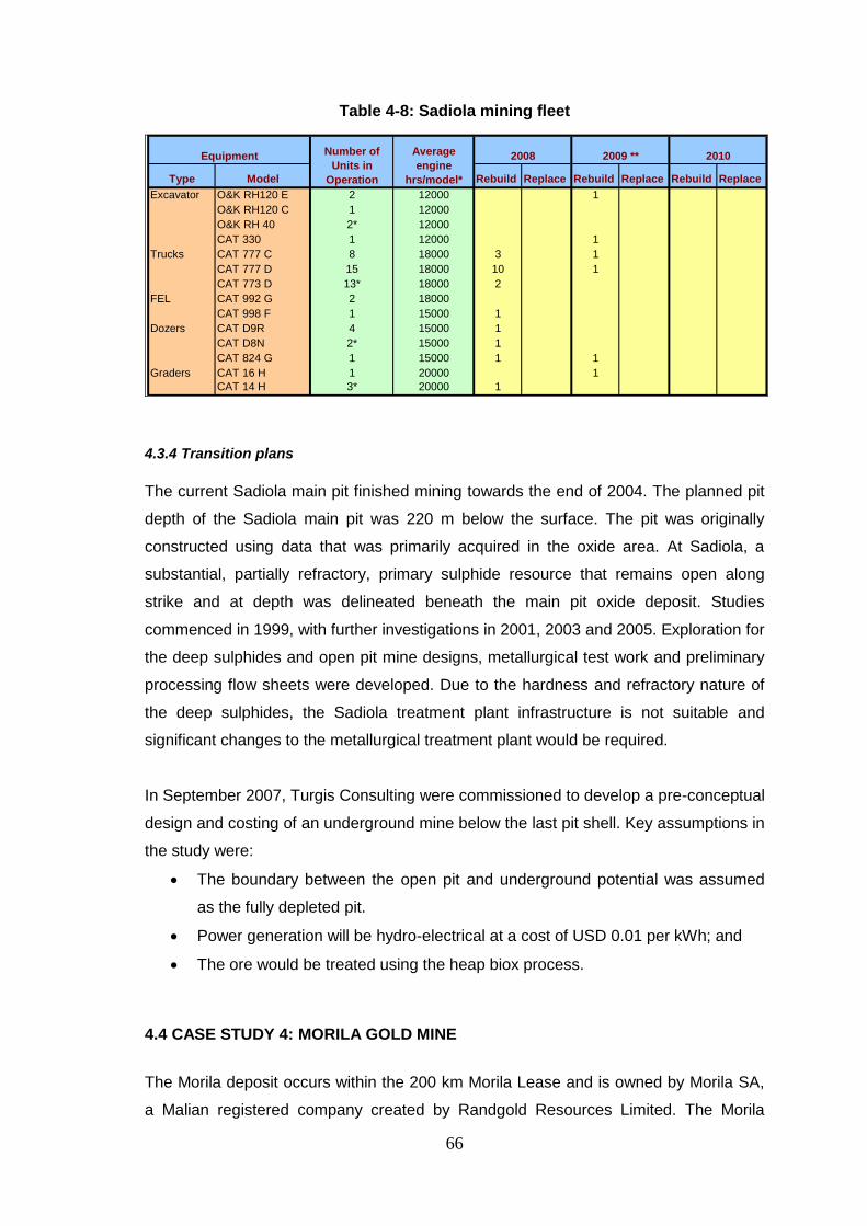
Table 4-10: Morila Mining fleet ....................................................................................70
Table 4-11: Summary of rock types in the resource model ..........................................70
Table 4-12: Mining production statistics .......................................................................70
Table 5-1: Chronological list of events at Sunrise Dam Gold Mine ..............................74
Table 5-2: SDGM 1996-2002 production summary......................................................75
Table 5-3: Comparisons of mine statistics for the case study mines (Courtesy:
AngloGold Ashanti) .....................................................................................................77
Table 5-4: Key transition indicators for base model .....................................................92
Table 5-5: Key transition indicators for simulated models ............................................92
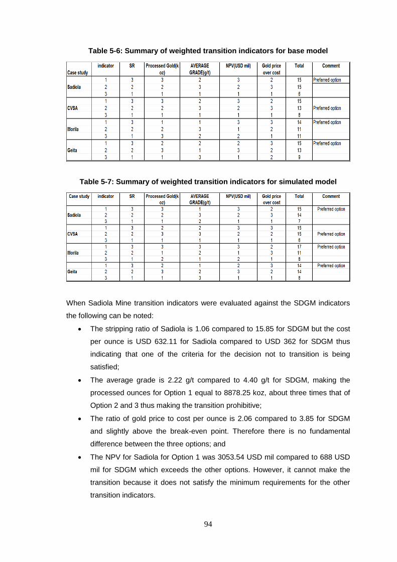
Table 5-6: Summary of weighted transition indicators for base model .........................94
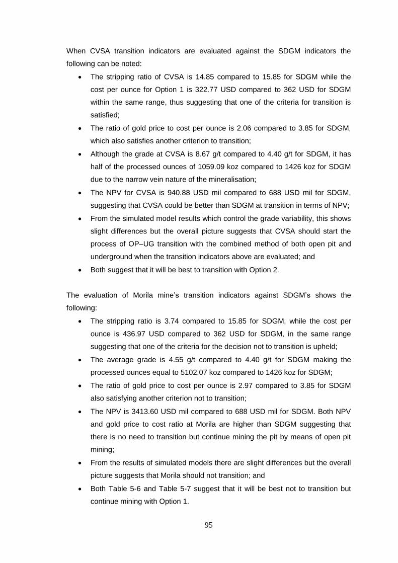
Table 5-7: Summary of weighted transition indicators for simulated model ..................94
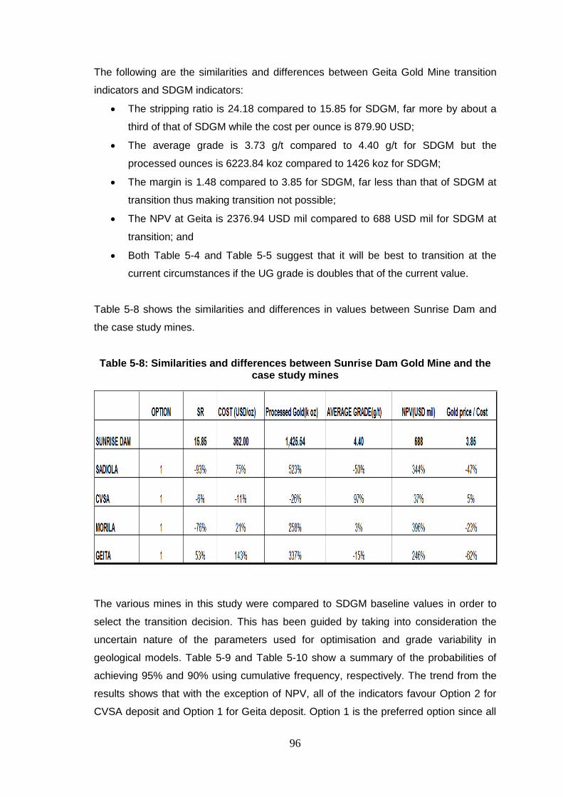
Table 5-8: Similarities and differences between Sunrise Dam Gold Mine and the case
study mines .................................................................................................................96
Table 5-9: Transition indicator values at 95% cumulative probability ...........................97
Table 5-10: Transition indicator values at 90% cumulative probability .........................97
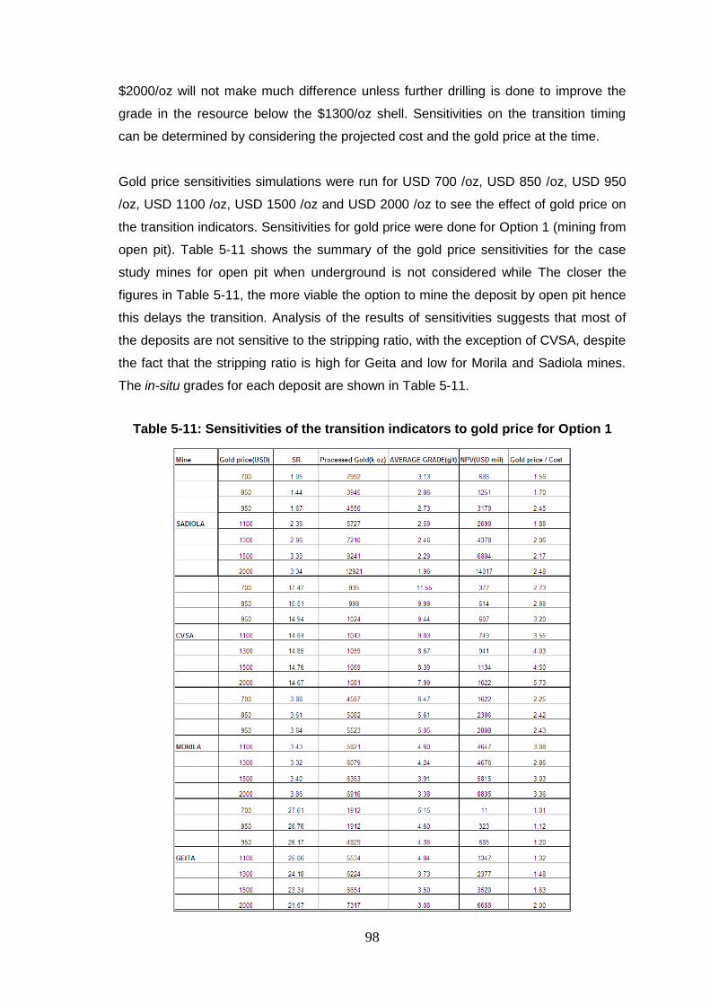
Table 5-11: Sensitivities of the transition indicators to gold price for Option 1..............98
Table 5-12: OP-UG transition indicators in relation to baseline values.........................99
Page 18
xvii
LIST OF UNIT SYMBOLS
Billion Years ............................................................................................................... Ga
Million Ounces ......................................................................................................... Moz
Million Tonnes .............................................................................................................Mt
Ounces ....................................................................................................................... oz
Thousand Ounces .................................................................................................... koz
US Dollar ................................................................................................................. USD
Australian Dollar ......................................................................................................... A$
Billion ..........................................................................................................................bn
Page 19
xviii
ABBREVIATIONS
AGA ...................................................................................... AngloGold Ashanti Limited
BCM .................................................................................................... Bank cubic metre
BIF ............................................................................................ Branded Iron Formation
BIFC .......................................................................................................... Chemical BIF
BIFS ..................................................................................................... Sedimentary BIF
BUP .................................................................................................. Business Planning
CAR ....................................................................................... Continental Africa Region
COV ............................................................................................. Coefficient of variation
DBSIM ....................................................................... Direct-block conditional simulation
EW ......................................................................................................... Equal Weighted
GMP ......................................................................................... General Mining Package
Htd ......................................................................................................... Transition depth
Htp .......................................................................................................... Transition point
IRR .............................................................................................. Internal Rate of Return
KPI ...................................................................................... Key Performance Indicators
LoM .............................................................................................................. Life of Mine
MCF ...................................................................................................... Mine Call Factor
MRO .................................................................................. Mineable Reserve Optimiser
NPU ............................................................................................. Near Pit Underground
NPV .................................................................................................. Net Present Value
NQ ........................................................................ Diamond drill core of 53mm diameter
OP - UG ................................................................................... Open pit to Underground
OP ..................................................................................................................... Open pit
ORD ...................................................................................... Ore Reserve Development
RUC ..................................................................................... Reverse Circulation Drilling
SD .................................................................................................... Standard Deviation
SGS ............................................................................. Sequential Gaussian Simulation
SIBC ........................................................................................ Stay in Business Capital
SMU ............................................................................................... Smallest Mining Unit
SR ............................................................................................................. Stripping ratio
TL ............................................................................................................ Transition level
UC ..................................................................................................Uniform Conditioning
UFS ................................................................................. Underground Feasibility Study
UG ............................................................................................................. Underground
Page 20
1
1.0 INTRODUCTION
Open pit mining is generally considered to be more advantageous as compared to
underground mining due to its mass production and minimum cost. If an ore body is
large and extends from surface to “great depth”, the part of the deposit close to the
surface is usually mined from an open pit to give early revenue while preparations are
being made for mining the deeper parts by underground means. Many surface mines
are increasingly becoming aware of the value gained by considering underground
options early in the open pit mining life. The choice of mining method and open-pit limit
for a specific mineral deposit depends on factors such as the geological conditions of
the ore body, stripping ratio, extraction depth and economic, community, social and
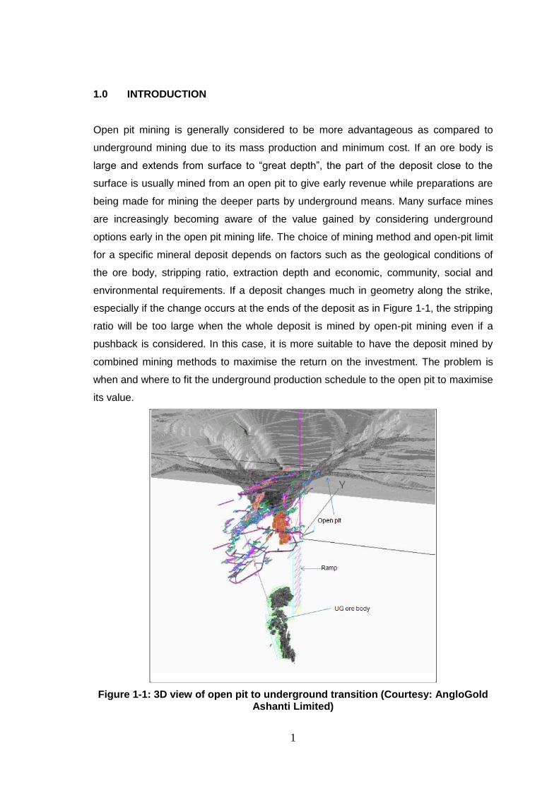
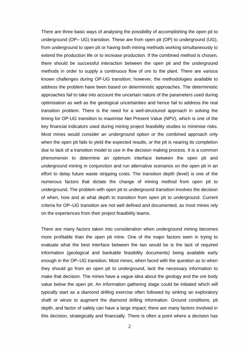
environmental requirements. If a deposit changes much in geometry along the strike,
especially if the change occurs at the ends of the deposit as in Figure 1-1, the stripping
ratio will be too large when the whole deposit is mined by open-pit mining even if a
pushback is considered. In this case, it is more suitable to have the deposit mined by
combined mining methods to maximise the return on the investment. The problem is
when and where to fit the underground production schedule to the open pit to maximise
its value.
Figure 1-1: 3D view of open pit to underground transition (Courtesy: AngloGold Ashanti Limited)
Page 21
2
There are three basic ways of analysing the possibility of accomplishing the open pit to
underground (OP– UG) transition. These are from open pit (OP) to underground (UG),
from underground to open pit or having both mining methods working simultaneously to
extend the production life or to increase production. If the combined method is chosen,
there should be successful interaction between the open pit and the underground
methods in order to supply a continuous flow of ore to the plant. There are various
known challenges during OP-UG transition; however, the methodologies available to
address the problem have been based on deterministic approaches. The deterministic
approaches fail to take into account the uncertain nature of the parameters used during
optimisation as well as the geological uncertainties and hence fail to address the real
transition problem. There is the need for a well-structured approach in solving the
timing for OP-UG transition to maximise Net Present Value (NPV), which is one of the
key financial indicators used during mining project feasibility studies to minimise risks.
Most mines would consider an underground option or the combined approach only
when the open pit fails to yield the expected results, or the pit is nearing its completion
due to lack of a transition model to use in the decision making process. It is a common
phenomenon to determine an optimum interface between the open pit and
underground mining in conjunction and run alternative scenarios on the open pit in an
effort to delay future waste stripping costs. The transition depth (level) is one of the
numerous factors that dictate the change of mining method from open pit to
underground. The problem with open pit to underground transition involves the decision
of when, how and at what depth to transition from open pit to underground. Current
criteria for OP–UG transition are not well defined and documented, as most mines rely
on the experiences from their project feasibility teams.
There are many factors taken into consideration when underground mining becomes
more profitable than the open pit mine. One of the major factors seen in trying to
evaluate what the best interface between the two would be is the lack of required
information (geological and bankable feasibility documents) being available early
enough in the OP–UG transition. Most mines, when faced with the question as to when
they should go from an open pit to underground, lack the necessary information to
make that decision. The mines have a vague idea about the geology and the ore body
value below the open pit. An information gathering stage could be initiated which will
typically start as a diamond drilling exercise often followed by sinking an exploratory
shaft or winze to augment the diamond drilling information. Ground conditions, pit
depth, and factor of safety can have a large impact; there are many factors involved in
this decision, strategically and financially. There is often a point where a decision has
Page 22
3
to be made whether to continue deepening the mine or changing to underground
methods. The question most mines face is why one has to evaluate an underground
mining method in an early stage of the open pit planning or during open pit production.
However, the reality is that the economic final pit is usually closer than one thinks.
Perhaps one of the most important decisions, in the initial stages of a project for a
transition from open pit to underground mining, is the definition of the most suitable
underground mining method based on the characteristics of the deposit and, at the
same time, the economic and business requirements of the mining company. Business
requires high production rates and low operational costs. In choosing between OP and
UG, the time to transition is critical to maximise the value of the resource. A well-
balanced schedule needs to be maintained during the transition period to maintain a
constant production profile.
There are opportunities to add value if the timing of the underground and open pit
mining fits appropriately into the company’s strategic plan. Proper planning during open
pit to underground transition is done with the aim of optimising mineral production and
rationalising waste stripping to manage the stripping ratio, and thereby reducing the
operating and capital costs. In addition, mining fleet rationalisation during the transition
is prepared to ensure the best fit-for-purpose and cost effective fleet to be utilised. In
making a choice between OP and UG, the time to transition is vital to maximise the
value of the resource and to keep the window of opportunity opened. Comprehensive
budgeting, anchored on good operating, capital cost estimates and proper scheduling
of the expenditures, and timely execution of plans in each department and section are
necessary in order to achieve a good transition. In mining, the capacity determines the
rate of extraction and hence exhaustion of the reserve. Thus, there is usually an
interaction between the capacity decision and the production decisions. An
underground mine requires large up-front capital in the form of shaft access,
development and equipment, and the cost can be in the order of billions of United
States Dollars (USD). Obtaining approval for this kind of money requires
comprehensive information to justify a big upfront spend of capital.
To deepen an open pit beyond its ultimate depth is expensive and time consuming
given that the stripping ratio will change as the pit deepens. Every mine and its deposit
are unique but there are common factors such as those encountered in diamond pipes.
The underground mine will normally be directly underneath the open pit whereas in
copper, gold and other deposits there might be enough space available to locate the
underground mine away from the open pit. Many factors affect the decision on whether
Page 23
4
to commence a mine as an open pit (OP), underground (UG) or transition from open pit
to underground (OP-UG) at a later stage. Some of the impacts include the cost of
stripping which may reduce cash flow from the operation and may not be strategically
desirable at the beginning of the project.
Vertical narrow vein ore bodies are more suitable to underground mining, whereas
open pits have high stripping ratios. On the other extreme, large porphyry ore bodies
can be mined at a very low cost by open pit if they are close to the surface. For
complex ore bodies (geology not well understood), open pit resource recovery can
make the open pit cheaper than underground mining as generally all rock within the pit
shell is mined. In an open pit, the ore can be separated through the grade control
process, but in an underground mining scenario, mining costs are higher and the goal
is to minimise waste mining – this means that smaller areas of ore that can be mined
by open pit may be left in an underground scenario, usually as pillars. In UG mining,
the mining is not done from top down (as in a pit) and would be more selective. If the
mine is mill constrained, there is an opportunity to “high grade” the mine at the
beginning of the mine life to allow higher cash flows. If resource recovery is not a
requirement then the cut-off grade is lifted in order to lift the head grade. An open pit
exposes the ore whereas in underground mining it is easier to limit access. When a pit
goes deeper the stripping ratio increases, mining costs escalate with depth, haulage
distances increase, wear and tear on the equipment (truck tyres) increases. The rock
conditions change as the pit gets deeper resulting in tighter blast patterns, which
increase blasting costs, more groundwater, and surface water needs to be pumped out,
profit margin begins to decline and the incremental value of the pit gets smaller
(www.gemcomsoftware.com).
1.1 Background information
Many open pit mines are planning or implementing the process of open pit to
underground transition and many of them have encountered problems during the
implementation stage of the transition processes after feasibility studies and have not
been able to follow their feasibility plans to the end. Some of these mines include
Palabora, Finsch and Venetia in South Africa; Bingham Canyon in the USA;
Chuquicamata and Mansa Mina in Chile; Grasberg in Indonesia; Kidd Creek Mine,
Doyon Gold Mine, and Dome Mine in Canada; Jwaneng Mine in Botswana; Telfer,
Argyle, Mount Keith and Sunrise Dam in Australia and Geita Mine in Tanzania. Some
OP-UG transition problems include instability in the areas closer to the underground
Page 24
5
operation, deteriorating haulage roads, increasing probability of slope failures and
unsafe working conditions and underground flooding due to the groundwater and/or
surface water inflow.
1.1.1 Status of some open pit to underground transition mines
A mine can be a surface (strip mine or an open pit mine) or an underground mine. The
mining method used depends on the depth, lateral extent and economic value of the
ore being mined. The deepest underground mine is in West Wits (about 3.5 km), a
South African gold mine, while an open-pit Bingham Canyon Mine is more than 4 km
wide and more than 1 km deep. The shape of a mineral deposit (small, irregular,
deeply buried, narrow, vein) mostly dictates the choice between open pit and
underground mining. In 1955, Butte mine in the USA began the transition from
underground to open pit. Butte mine is among few mines to transition from
underground to open pit. Palabora mine in South Africa had to transition from open pit
to underground using the block caving mining method when the pit reached 800 m
depth. Doyon Mine began the open pit mine in 1980 and commenced the underground
in 1985. Table 1-1 shows a status of some open pit to underground transition mines.
Page 25
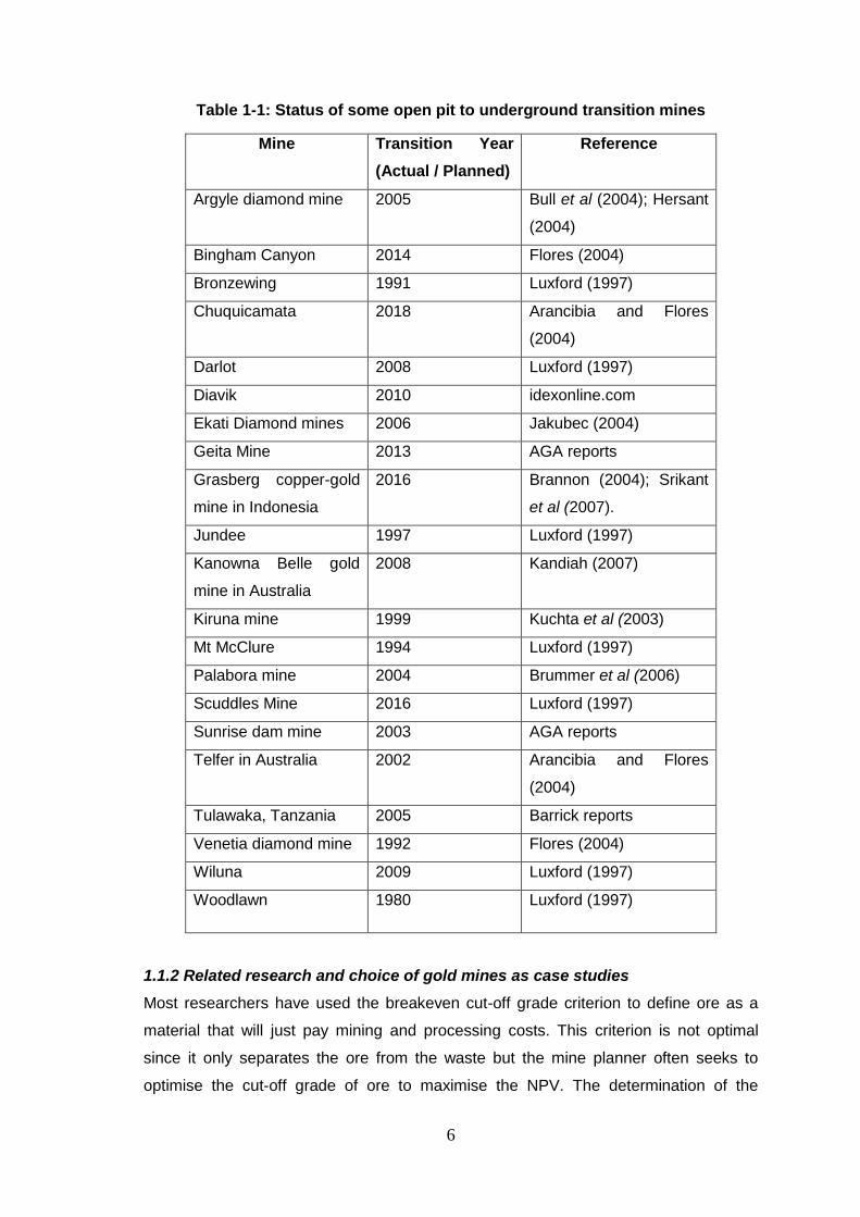
6
Table 1-1: Status of some open pit to underground transition mines
Mine Transition Year
(Actual / Planned)
Reference
Argyle diamond mine 2005 Bull et al (2004); Hersant
(2004)
Bingham Canyon 2014 Flores (2004)
Bronzewing 1991 Luxford (1997)
Chuquicamata 2018 Arancibia and Flores
(2004)
Darlot 2008 Luxford (1997)
Diavik 2010 idexonline.com
Ekati Diamond mines 2006 Jakubec (2004)
Geita Mine 2013 AGA reports
Grasberg copper-gold
mine in Indonesia
2016 Brannon (2004); Srikant
et al (2007).
Jundee 1997 Luxford (1997)
Kanowna Belle gold
mine in Australia
2008 Kandiah (2007)
Kiruna mine 1999 Kuchta et al (2003)
Mt McClure 1994 Luxford (1997)
Palabora mine 2004 Brummer et al (2006)
Scuddles Mine 2016 Luxford (1997)
Sunrise dam mine 2003 AGA reports
Telfer in Australia 2002 Arancibia and Flores
(2004)
Tulawaka, Tanzania 2005 Barrick reports
Venetia diamond mine 1992 Flores (2004)
Wiluna 2009 Luxford (1997)
Woodlawn 1980 Luxford (1997)
1.1.2 Related research and choice of gold mines as case studies
Most researchers have used the breakeven cut-off grade criterion to define ore as a
material that will just pay mining and processing costs. This criterion is not optimal
since it only separates the ore from the waste but the mine planner often seeks to
optimise the cut-off grade of ore to maximise the NPV. The determination of the
Page 26
7
optimum cut-off grade for a single metal deposit can be very complex even when price
and cost are assumed to be constant. This is because it involves the costs and
capacities of the several stages of the mining operations, the waste/ore ratios and
average grades of different increments of the ore body. If mineralisation extends
beyond a certain depth from the surface of a pit, the stripping ratio (SR) becomes too
high. It should then be converted to an UG mine. Optimisation of the transition problem
was, and still is, an important issue in mining.
This thesis modelled the open-pit to underground transition problem, which was
researched from a stochastic or probabilistic point of view by developing a model for
mining companies to transition decisively and smoothly. Sometimes, mining companies
are forced to simplify their operations, and tend to make simple statements of how
many tonnes of a certain grade they can produce (and market what they can sell).
Therefore, it is common in open pit gold mines to work with fixed stripping ratios, cut-off
grades, beneficiation rules and product specifications. The challenge is now for mining
organisations to see how quickly they can step up their management processes to see
exactly what their resources are actually capable of delivering.
Information gathering for OP-UG transition is a difficult task. The reserves for various
companies are generated from resource models. Most mining companies have a
confidentiality associated with them making it impossible to obtain geological models.
Data from gold mines in only one mining company (AngloGold Ashanti Limited), the
researcher’s employer, that have had to change their transition plans since there was
no model to follow to assess OP-UG transition, were used for the study. The time
involved in running a model to generate the transition indicators for each of the four
case study mines was about nine months. This time constraint limited this study to four
case study mines, although AngloGold Ashanti Limited, one of the world’s leading gold
mining companies, has 21 operations in 10 countries on four continents.
1.2 Research question
There are few methods available to mining companies in making the decision as to
when to transition from open pit to underground. The most common one is by
comparing the differences in the financial returns of a pushback, to mining the same by
underground means, using optimisation software such as Minemax (global optimiser
that seeks to maximise NPV). Most of the studies done on open pit to underground
transition were based on the transition depth (Htd). However, this is inadequate
Page 27
8
because as indicated earlier, there are other factors that are critical to the transition
decision. These factors change over time and make the transition depth dynamic or
uncertain hence the hesitation or delays by mines to make the transition. The question
is therefore:
“Is there a set of appropriate criteria or indicators that can be utilised to trigger
the transition decision from open pit to underground mining given the
uncertainties in the geological models, gold price as well as cost and
processing recoveries?”
1.3 Statement of objectives of the thesis
The main objectives of this research were to:
Identify appropriate transition indicators for open pit to underground transition;
Develop a stochastic model using transition indicators based on grade or
geological uncertainty for the open pit to underground transition. This model will
help reduce possible loss of the huge capital investment during OP-UG
transition and enhance surface and underground mine planning processes by
incorporating more flexibility in the planning process; and
Test the OP–UG transition model using baseline values.
1.4 Research methodology
The methods employed in this study included:
Collection, extraction, collation and validation of geotechnical data, mining data,
and geological models on the various mine sites;
Testing of OP – UG transition model using values of transition indicators for
Sunrise Dam Gold Mine as baseline values;
Analytical and statistical evaluation of the results; and
Comparing the OP – UG results against industry norms.
1.5 Problem formulation
Uncontrollable parameters in OP to UG transition include:
Gold price;
Ore body geometry, and
Page 28
9
Infrastructure (location of the mine).
Controllable parameters in OP to UG transition include:
Mining method;
Timing (window of opportunity);
Cost, plant recoveries, mine call factor (MCF);
Cut-off grade; and
Stripping ratio.
One way to determine OP-UG transition is to convert the open pit pre-stripping ratio of
cost per tonne and compare the value to the underground mining cost. This is the
standard financial analysis approach. This is different for each ore body. Transitioning
from open pit to underground may change the mine from a mill-constrained scenario to
a mining constrained one when mining underground only.
Most transition mines have faced one problem after the transition. Some of the factors
contributing to the transition problem are as follows:
The effect of change in the gold price and cost;
Ability to maintain the required plant throughput during and after
transition;
Geotechnical challenges and stability of the rock mass;
Lack of confidence in the geological resource model;
Environmental factors like subsidence, which sometimes favour open pit
rather than underground mining;
Lack of expertise to make the transition; and
Capital required to transition.
1.6 Thesis structure
The structure of the thesis is illustrated in Figure 1-2. There are six chapters. Chapter 1
introduces the thesis work which clearly states the research question, the problem
definition, objectives, methodologies applied to achieve the objectives, scope of work,
as well as the organisation of the report. Chapter 2 reviews the OP - UG transition
literature. The modelling process in solving the OP - UG transition problem and the
conceptual transition model are explained in Chapter 3. Chapters 4 discuss the four
case study mines in this particular order: Geita, Cerro Vangudia SA, Sadiola Gold Mine
Page 29
10
and Morila Gold Mine. Chapter 5 analyses the Sunrise Dam Gold Mine to provide
baseline values for the model and lastly, Chapter 6 has the conclusions and
recommendations based on the results of the study.
Figure 1-2: Layout of thesis structure
Page 30
11
2.0 REVIEW OF OPEN PIT TO UNDERGROUND TRANSITION
Open-pit mining is generally preferred by most mine planners and investors compared
to underground mining where an ore body is located close to the surface, large enough
and has little overburden. Underground mining options for extraction are considered at
a point in the mining life when economic conditions become impossible to continue
mining using open pit methods. At this point, comparisons are made between mining
the deposit by open pit or underground. The point at which the mining method is
changed from open pit to underground is often referred to as the transition point (Htp) or
transition depth (Htd). The transition point could occur anywhere from pre-feasibility
project stage to years after commencement of mining. The transition point at which an
underground mine becomes more economic than an open pit operation is not a single
evaluation but depends on many factors. It is therefore more reasonable to refer to a
transition point rather than transition depth.
For an outcropping ore body, it is best to be mined by open pit down to the point where
the cost of mining the last tonne is equal to the cost of mining that tonne from
underground. The last cut in the open pit is generally marginal while the first production
from underground is the most costly because it will take months to develop the
sequence of stoping required to meet full production capacity. One of the most
important decisions in the initial stages of a mining project is the choice of a suitable
mining method (open pit or underground) based on the characteristics of the deposit
and the economic and business requirements of the mining company. If the business
requires high production rates and low operational costs, then the method could
include an open pit mining or an underground caving mining method.
Factors that affect the ideal transition from OP to UG mining are cut-off grades, waste
stripping, portability of skills from surface mining experience to underground mining
environment, stockpile generation and reclamation, capital requirements, tailings
capacity, closure cost implications, as well as the decision of what depth and when to
make the transition. Currently, the criteria for making this transition are not well defined.
Some of the factors that can affect OP-UG transition can be listed as follows:
UG cost (sensitive to depth);
Time to transition is critical to maximise the value;
Mining cost (determines when to transition);
Page 31
12
Stripping ratio (required break even to transition);
Huge capital required for UG project;
Unit cost of surface mining (increases with depth due to amount of waste to be
removed);
Ore body configuration determines how to transition (size of the deposit and
final pit slope angle);
Types of material found below a certain depth and the availability of the
processing methods for treatment or modification on the existing plant
constrains UG transition;
Decisions as to how and when to act including the extraction and routing of
blocks of ore, the timing of decisions such as pushback or transitions;
The placement of shafts; the ratio of ore to waste in OP controls the transition
level; Open pit should mine ore bodies whose stripping ratio (SR) does not
exceed the break even stripping ratio;
Conversion of mining equipment from OP to UG mining;
High risk assessments in OP mining constrained pits to be mined below certain
depths and transition is therefore required earlier than anticipated; and
The depth at which free cash flow becomes negative.
2.1 Previous research on open pit to underground transition
The following section details work done by other authors in trying to address the OP-
UG transition decision. Among various parameters considered by the authors were
cost, stripping ratio, transition depth, geotechnical challenges and using Gemcom’s
Whittle 4X software as a tool to assess if going underground is feasible
(www.gemcomsoftware.com).
2.1.1 Cost and stripping ratio
Luxford (1997) briefly discussed some of the issues involved in making the transition
from open pit to underground mining. His aim was to flag the critical issues when
planning to make the transition from open pit to underground mining and to identify
critical aspects of mine development. Luxford (1997) discussed the OP-UG transition
issues, with emphasis on gold and copper deposits in Australia. He said that many
open cast mines were developed on shallow oxide reserves but have exhausted these
Page 32
13
reserves and these mines have made the transition to the deeper sulphide ore whilst
some of the operations have reached a point where decisions will soon have to be
made to transition from OP–UG mining. Luxford (1997) made the following points:
Mining companies use open pit-mining methods if the reserves are in the
shallow oxides because the oxide rocks are mostly soft and cannot support
underground mining;
Cost usually drives the decision to take an open pit mine underground. He
argued that as open pit stripping cost keeps rising, as the mine gets deeper,
there comes a time when underground mining cost will be less than the open pit
mining cost. At that point, which this research proposes as transition point (Htp),
a decision to choose between extending the open pit mine and going
underground is made after considering detailed analysis of all operational and
capital costs; and
Capital costs are often a factor in the choice between a major pushback and
going underground. It seems reasonable that cost is one of the many factors
that determine the OP-UG transition. Open pit mining should continue until the
underground mining cost becomes cheaper than the open pit mining cost
before the detailed cost analysis is made.
However, Luxford (1997) did not mention the mining method being used to exploit
the sulphide ore neither did he show how the open pit and underground cost could
be calculated in making the transition decision. Luxford’s views on the following are
still applicable:
Workforce recruitment;
Ore body geometry;
Ore handling;
Production rate;
Decline, conveyor or shaft;
Ventilation, and
Geomechanics.
Page 33
14
2.1.2 Transition depth and its determination
Hayes (1997) discussed the impact, which makes UG mining more economic than OP
mining and noted the importance of issues such as management competence and
system, geological setting, geotechnical characteristics, stripping ratio, productivity and
capital cost in making this decision. He included the following factors in determining the
transition depth as: the mineral resource, the mining method and the mining cost
factors.
Finch (2012) stated that the OP-UG transition problem manifests itself in two ways.
These are sequential and parallel mining. In the sequential mining, the UG mining is
directly beneath the open pit, whereas with the parallel mining there is an opportunity to
site the underground portion away from the open pit mining allowing for simultaneous
mining of both the OP and the UG. Finch (2012) argued that to determine the optimal
transition point the following issues need to be evaluated:
Availability of feed;
Feed grade;
Resource utilisation impact;
Stripping ratio;
Price;
Production rate; and
Mining cost.
Finch (2012) dwelled much on the transition point evaluation so that the point that
offers the higher values can be chosen. The point Finch (2012) made was valid
however, the transition point cannot be complete until a point in time is determined
since the factors involved in its determination change over time.
The model for determining the optimal transition depth from open pit to underground
mining by Bakhtavar et al (2008) stated that the most significant problem at that time
was the determination of optimal Transition Depth (Htd) from OP to UG mining.
Bakhtavar et al (2008) used a heuristic algorithm as a basic model based on Block
Economic Value of OP and UG. They derived their formulae based on the allowable
and overall stripping ratios. For this objective, an analytical procedure was produced.
The contemplated model is about deposits with outcrops or overburden and including
Page 34
15
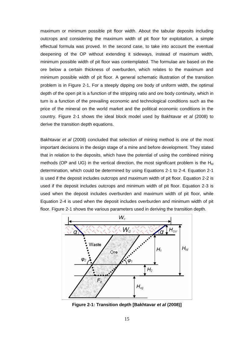
maximum or minimum possible pit floor width. About the tabular deposits including
outcrops and considering the maximum width of pit floor for exploitation, a simple
effectual formula was proved. In the second case, to take into account the eventual
deepening of the OP without extending it sideways, instead of maximum width,
minimum possible width of pit floor was contemplated. The formulae are based on the
ore below a certain thickness of overburden, which relates to the maximum and
minimum possible width of pit floor. A general schematic illustration of the transition
problem is in Figure 2-1. For a steeply dipping ore body of uniform width, the optimal
depth of the open pit is a function of the stripping ratio and ore body continuity, which in
turn is a function of the prevailing economic and technological conditions such as the
price of the mineral on the world market and the political economic conditions in the
country. Figure 2-1 shows the ideal block model used by Bakhtavar et al (2008) to
derive the transition depth equations.
Bakhtavar et al (2008) concluded that selection of mining method is one of the most
important decisions in the design stage of a mine and before development. They stated
that in relation to the deposits, which have the potential of using the combined mining
methods (OP and UG) in the vertical direction, the most significant problem is the Htd
determination, which could be determined by using Equations 2-1 to 2-4. Equation 2-1
is used if the deposit includes outcrops and maximum width of pit floor. Equation 2-2 is
used if the deposit includes outcrops and minimum width of pit floor. Equation 2-3 is
used when the deposit includes overburden and maximum width of pit floor, while
Equation 2-4 is used when the deposit includes overburden and minimum width of pit
floor. Figure 2-1 shows the various parameters used in deriving the transition depth.
Figure 2-1: Transition depth [Bakhtavar et al (2008)]
Page 35
16
AC
CRCRWH
w
opopugugd
td
Equation 2-1
AC
CFWCCRWH
w
wpdopugugd
td
Equation 2-2
ABC
AFWCABCRCRWH
w
pdwopopugugd
td
2
2 Equation 2-3
ABC
AWWCABCRCRWH
w
dcwopopugugd
td
2
2 Equation 2-4
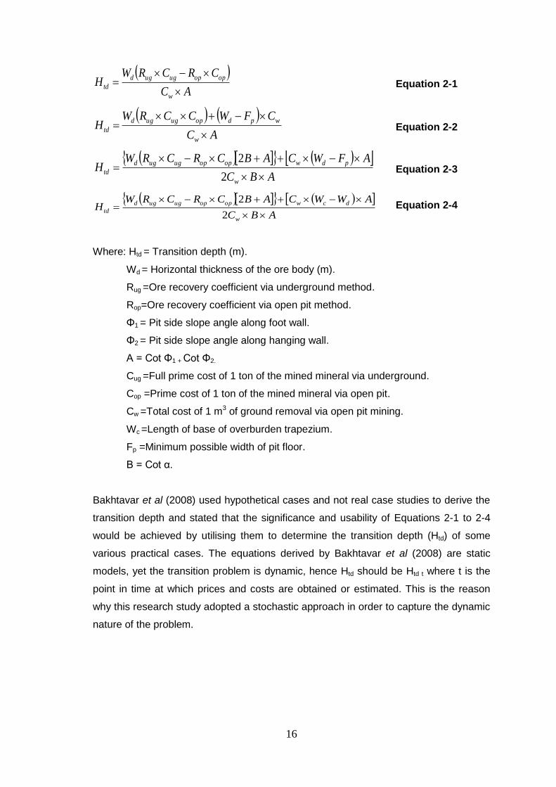
Where: Htd = Transition depth (m).
Wd = Horizontal thickness of the ore body (m).
Rug =Ore recovery coefficient via underground method.
Rop=Ore recovery coefficient via open pit method.
Φ1 = Pit side slope angle along foot wall.
Φ2 = Pit side slope angle along hanging wall.
A = Cot Φ1 + Cot Φ2.
Cug =Full prime cost of 1 ton of the mined mineral via underground.
Cop =Prime cost of 1 ton of the mined mineral via open pit.
Cw =Total cost of 1 m3 of ground removal via open pit mining.
Wc =Length of base of overburden trapezium.
Fp =Minimum possible width of pit floor.
B = Cot α.
Bakhtavar et al (2008) used hypothetical cases and not real case studies to derive the
transition depth and stated that the significance and usability of Equations 2-1 to 2-4
would be achieved by utilising them to determine the transition depth (Htd) of some
various practical cases. The equations derived by Bakhtavar et al (2008) are static
models, yet the transition problem is dynamic, hence Htd should be Htd t where t is the
point in time at which prices and costs are obtained or estimated. This is the reason
why this research study adopted a stochastic approach in order to capture the dynamic
nature of the problem.
Page 36
17
2.1.3 Geotechnical challenges
Flores (2004) pointed out some of the geotechnical challenges associated with caving
during open pit to UG transition by using Chuquicamata mine as a case study. This
was carried out through the International Caving Study Stage II (ICS-II), managed by
the Julius Kruttschnitt Mineral Research Centre, Brisbane, Australia, of which
CODELCO is one of the sponsors. That study concluded that there is currently neither
sufficient experience in transition for deep pits nor available design methodologies in
spite of the topic’s importance to the mining industry. The only documented transition
available at that time involving a large open pit and underground mining by caving was
Palabora mine, South Africa (Glazer and Hepworth 2004). Figure 2-2 shows the crown
pillar development from the open pit to underground transition at Chuquicamata mine.
Some of Flores findings were as follows:
When the final pit is reached in 2013 with a depth of 1,100 m, the undercut level
will be located at a depth of around 1,500 m from surface;
Cave initiation and propagation. The initial stage of the underground mining will
be in a hard and massive rock mass, where cave initiation and propagation may
be difficult;
Simultaneous open pit and underground mine operations. The economic and
business requirements of Chuquicamata mine are such that a period of
simultaneous open pit and underground mining would be required. Hence, at
least for a certain period, a stable crown pillar must be maintained between the
cave back and the pit bottom;
Subsidence, once the caving connects to the pit bottom the pit will become a
subsidence crater with a zone of influence extending beyond the pit perimeter;
and
Groundwater, due to the presence of groundwater in the slopes of
Chuquicamata’s open pit and some rains during the Bolivian winter (January
and February), there is a non-zero probability of inrushes of water or mud into
the underground mine. These inflows or mud-rushes could be worsened by the
presence of major geological structures.
Page 37
18
Figure 2-2: Surface crown pillar developed in a transition from open pit to underground cave mining (Flores, 2004)
Flores (2004) stated that the decision to make the transition from open pit to an
underground operation is often based on a simple determination of the NPV of the next
feasible open pit pushback. Underground mining is only contemplated when a further
pushback is shown to be uneconomic and stated that any decision to go underground
also requires consideration of a wide range of technical factors, and careful planning.
This means a significant amount of time is needed for achieving underground mining
and up to 20 years was suggested by Stacey and Terbrugge (2000).
Stacey and Terbrugge (2000) suggested that the transition problem was known but the
lack of a model to address the timing remained an issue. In such cases, it is desirable
that the open pit continues its operation during the first stages of underground mining,
and that the underground mine gets to a high level of productivity quickly before
closure of the open pit operation. This means that there will be a period of
simultaneous open pit and underground mining operations. Flores (2004) stated that
the simultaneity implies an interaction between the open pit and underground mining,
which makes the problem more complex than the typical open pit or underground mine
designs. The presence of the deep open pit will affect the stress field in which the
underground mine will be developed and, conversely, the propagation of the caving will
affect the stability of the surface crown pillar that defines the bottom of the open pit.
Additionally, many other factors or potential hazards could make the problem even
more difficult if these are not identified prior to making the transition from open pit to
underground mining.
Page 38
19
Stacey and Terbrugge (2000) highlighted that the following aspects must be
considered during the OP-UG transition:
The planning and implementation period for transition from OP-UG could take
as long as 20 years. In addition, they suggested that the planning must
commence at an early stage, which is indeed true requiring annual reviews of
the OP – UG transition decision;
An economically designed pit, should have slopes that are close to their stability
limits and little scope for extending the open pit mining to greater depths, other
than with a pushback;
Surface and underground infrastructure is often at risk due to deepening of pits,
underground mining below pits, and deepening of underground mining beyond
planned depths;
Introduces the risk of mud rushes from within the rock mass;
Air blasts occurs because of underground collapses in association with mud
rushes;
The presence of an abandoned pit above underground workings can lead to
greater risks of dilution and mud rushes; and
The choice of underground mining method has a major effect on the stability of
the surface.
Although Stacey and Terbrugge (2000) suggested transition timing up to 20 years they
did not provide any transition criteria to guide the OP-UG transition.
2.1.4 Going underground
Fuentes (2004), in his paper on going to an underground (UG) mining method, stated
that some open pit (OP) engineers have analysed underground mining methods,
mainly because they are anticipating the end of the economic life of those operations in
the near future. In comparing OP to UG mining methods, he said block caving was one
of the lowest cost underground mining methods, which can compete with some open
pits because of the high production rates, levels of mechanisation and the cost level
that can be achieved. He said underground mining presents more technical risks than
open pit methods with the possibility of events such as air blasts, rock bursts and hang-
ups. These risks could be quantified and managed in a rational, technical and
reasonable way. He described some key issues regarding block caving, some basic
information requirements, cost trends, potential production capacity, management
Page 39
20
issues and the expected evolution of some techniques that could improve or solve
some of the main technical constraints of the method.
Fuentes (2004) questioned why one has to analyse how many years in advance are
available to consider an underground mining configuration, or why one should have to
evaluate an underground mining method in an early stage of the open pit planning.
Moreover, he posed a question: “Is it a crazy idea to analyse UG mining 10 years in
advance of the final pit achievement?”(Fuentes (2004) in Massmin 2004: 633). Fuentes
explained that traditionally the decision-making process in the open pit planning does
not take into account the opportunity cost associated with the underground exploitation
of the remaining resources left by an open pit design. Standard methodology considers
sequential pushback evaluation and identifying the expansion that maximizes NPV of
the design. Usually, until this time a break-even analysis (OP versus UG) was carried
out using a primary approach for the underground exploitation with big uncertainties
within the UG project basis. Fuentes (2004) said OP-UG transition is anticipated when
the economic life of the open pit operation is nearing its end. Considering what Fuentes
(2004) reported, it is however more appropriate that transition indicators are to be used
during the Life Of Mine (LoM) schedules and their annual reviews so that the window of
opportunity is not closed for the underground project and to derive maximum
capabilities from the ore bodies.
Araneda et al (2004) stated that an option of a combined open pit and underground
caving operation was the best long-term option to capture value. Araneda et al (2004)
presented the overall process, the final plan and discussed some challenging issues. El
Teniente is one of the largest known deposits of porphyry copper in the world and one
of the five divisions of Codelco, a Chilean state-owned company. It is situated 80 km
south of Santiago and 44 km up in the Andes mountains and comprises of mining,
processing and smelting facilities. At El Teniente over 1,100 million tonnes of ore were
mined out during almost 100 years of mining. The open pit is now in operation in the
north-west side of the deposit, letting the east and south side proceed with
underground mining.
He said the challenging issues regarding the open pit may be grouped into three main
categories of information, interaction and planning. Interaction of personnel is certainly
one of the most challenging aspects of the plan, and first among underground
disciplines, but also between the open pit and underground operations. Sequencing of
underground mining with the open pit mining was treated initially under a heuristic
Page 40
21
approach, however the complexity of the problem, and the fine-tuning required, forced
the mine planners to treat it in a more detailed way. A four dimensional model was set
up based on the 3D subsidence angles defining active caving zones and its evolution in
time (fourth dimension). Although Araneda et al’s (2004) assertion on sublevel caving
was true, the decision was based on one case study mine; however, the OP–UG
transition decision should be based on several case study mines in order to have a
suitable model.
2.1.5 Evaluation of technical and economic criteria involved in changing from
surface to underground mining
Musendu (1995) tried to establish a general approach to determine the optimum level
at which to change from surface mining to underground operations by comparing the
theoretical to optimum factors that affect the transition depth. Musendu (1995) focused
on the transition level at which open pit mining switches over to underground mining
methods. Some of the variables he considered as affecting the sensitivity of transition
depths were:
Grade;
Dip of the deposit;
Size of the deposit;
Underground recovery;
Underground dilution;
Underground production rate;
Surface production rate;
Surface fixed cost;
Underground fixed cost;
Surface waste cost;
Surface ore cost;
Underground variable cost;
Price;
Discount rate;
Inflation rate;
Plant recovery;
Slope angle; and
Taxation rate.
Page 41
22
Musendu (1995) stated that transition indicators are sensitive to the following mining
parameters:
Mining recovery: favours open pit than underground due to mass production in
the open pit;
Price and grade: higher price and higher grade favour open pit mining than
underground mining;
Cost (OP and UG):the higher the OP cost the better for UG;
Surface and underground variable ore cost: lower OP cost than UG cost
favours OP;
Cost of stripping waste: the higher this cost the earlier the transition;
Production rate: higher production rate favours open pit mining than
underground mining except when using the caving mining method; and
Underground dilution: impacts on transition depth by reducing the grade to the
plant.
Musendu (1995) considered most variables involved in the OP – UG transition but like
Bakhtavar et al (2008) based the transition problem on transition level; hence TL which
should be TLt, where t is the point in time at which the parameters are obtained (or
estimated).
The Pyhasalmi Mine is located in central Finland. The copper deposit was discovered
in 1958 (Kurppa and Erkkila, 1967). The ore obtained from open pit and underground
mining was being crushed by the same underground crushing facilities. The ore body
extends from the surface down to at least 500 m, the length is 650 m long, the central
part is 75 m wide and dips at 50°, 70° and 90° in different sections of the ore body as
illustrated in Figure 2-3.
Kurppa and Erkkila (1967) in their paper on changing from open pit to underground
mining at Pyhasalmi stated that a unique feature of the mine was the simultaneous
mining of the open pit and underground mining as well as the long transition period.
The geometry is suited for simultaneous OP-UG mining as shown in Figure 2-3. The
vertical position of the ore body and the fact that it extends sufficiently deep, meant that
inclined raises allowed them to direct the ore into the underground crushing plant. The
heavy rubber-wheeled equipment employed in the open pit gave such good results that
similar equipment was also used underground according to Kurppa and Erkkila (1967).
Page 42
23
About 25% of the production came from underground mining. The ore body was
covered by overburden of 2 to 3 m thick; hence open pit mining was the obvious choice
at the commencement of activities. However, the ore body extends deep in the ground
thereby allowing them to use underground mining methods for exploitation. It was
calculated for the open pit mining to have ore for ten years to serve the surface
operations and to allow early testing of the transition to underground mining. Waste
from the open pit was used as fill for the underground operations. A sufficiently early
commencement of underground stoping was to allow the dumping of waste from the
lower part of the pit directly into the stopes. The establishment of an experimental
stope under the open pit, the stability of which could be observed and used later for
testing of the filling operation, was also important. There was enough time for the
development of underground stoping. The area of the open pit was 56,000 m2, and the
pit was 330 m long and 225 m wide with average slope of the walls as 60º. Front-end
loaders were used to dump the ore into the ore passes situated at the bottom of the
pits at a depth of 200 m below surface. (Kurppa and Erkkila, 1967) made a valid point
that the ore body configuration dictated the obvious choice of the combined mining
method (both open pit and underground).
Figure 2-3: Geological sections for an ideal OP-UG transition (Kurppa and Erkkila, 1967)
Kurppa and Erkkila (1967) used the mine ore body’s configuration to prove their point,
which may not be used to generalise OP-UG transition. They also stated that the
transition from open pit to underground mining took place gradually over a period of
several years to ensure testing of the underground operation and to ensure smooth
Page 43
24
production. The reasons for the gradual change over of the OP–UG transition at
Pyhasalmi were valid but the time required for the transition could not be determined.
2.1.6 Underground mining: a challenge to established open pit operations
Arnold (1996) used the Barrick Bullfrog mine located about eight kilometres from
Beatty, Nevada, as a case study to state the inherent problems in starting and
operating an underground mine from an open pit mine. He stated that the ultimate pit
bottom is generally within 100 to 300 metres (300 to 1,000 feet) from the surface.
Arnold (1996) noted that the critical path in open pit mining flows through the drilling, to
design obtained from floating cone algorithm, but with underground mining, the ore
body is generally much deeper, and drilling it out to accommodate a full-scale design is
impractical. He stated that time is needed to take the drill data from a geologic model to
a mining plan. It has to include as much rock mechanics, ventilation, access design,
and mining method work as practical. Arnold (1996) proposed that, time was required
to drill out the underground resource but did not provide a solution to the inherent
problems and the transition timing.
2.2 Using Whittle software to determine when to go underground
Luxford (1997) stated that the commercially available computer programmes such as
Whittle 4D can now be used to determine where to make the transition from open pit to
underground mining and stated the assumption that these programmes can determine
the optimum final pit floor to about ± 20m accuracy. In 1998, Whittle programming
(Four-X) developed an open pit and underground mining interface in the optimisation
software to assist in the determination of the underground option, but the software
cannot be used to determine the period of time to transition. However, management
can make limited decisions based on quantified operational scenarios in the open pit to
underground transition. Whittle Four-X can indicate the point at which it becomes more
economically viable to proceed to underground mining, a decision which is difficult to
make by traditional methods. Some of Whittle’s (2009) suggestions regarding Whittle
software were as follows:
• Whittle can be used to determine the most profitable option: open pit or
underground;
• Whittle can be used to indicate at which point it becomes more economical to
proceed to underground mining;
Page 44
25
• Whittle cannot be used to determine whether it is worth going underground or
not;
• Whittle cannot be used to determine how much money can be gained from the
underground mine; and
• It cannot be used to optimise the underground operation, schedule underground
material, or include underground material in its results.
The enterprise optimisation is among the latest developments in optimisation in the
mining industry. It seeks to include most value and assets in the enterprise portfolio
and periods together including planning and modelling with uncertainty thereby making
the impact of uncertainty measurable, managed or exploited. Whittle’s (2009) theory of
Enterprise Optimisation defined 10 value levers driving the decision as follows:
Resource
Pit optimisation;
Pit phasing;
Mine schedule;
Cut-off grade and blending;
Stockpile;
Plant calibration;
Product (mix and specifications);
Logistics; and
Market.
Whittle (2009) did not consider the underground portion and hence Whittle software
remains an indicative tool for the transition to underground mining. The application of
the enterprise optimisation methodology will provide answers and guidance to relevant
questions to be answered. The enterprise optimisation has been introduced to reduce
the uncertainty in the open pit planning but did not address the OP-UG transition
timing. The question is at what point should open pit mine stop for the underground
mining to commence.
2.3. OP –UG transition framework
Figure 2-4 shows the interaction between open pit and underground mining during the
transition.
Page 45
26
Figure 2-4: OP – UG transition framework
The OP – UG transition decision entails inter-departmental interactions as shown in
Figure 2-4 to make the outcome of the transition decision acceptable to the
stakeholders. Among some of the interactions involved are the grade, geotechnical
properties of the rock and the mine reserves to generate the various models. UG
mining method selection and scheduling are iterative and could take time to reach an
optimum economic decision.
2.4. Checklist for OP-UG transition
The OP-UG transition model has the following characteristics:
• Gold as early as possible;
• Sound infrastructure with acceptable risk;
• Infrastructure must fit within a total infrastructure strategy capable of mining to
desired level;
• Seamless production between the phases; and
• The highest financial returns.
To have a sound OP - UG transition model, the following checklist was developed by
the researcher and requires questions to be answered during the data gathering phase
before the commencement of the project. The checklist will ensure that the OP-UG
Page 46
27
transition decision is not based on an individual effort but on a team effort since the
questions will involve expert input from more than three disciplines.
2.4.1 Geology
1. Is there an underground potential for the ore body?
2. Does the ore body extend beyond the current open pit surface?
3. What is the grade and depth of the ore body, which extends beyond the
current open pit surface?
4. What are the thickness, dip and strike of the deposit?
5. To which resource classification has the ore body been drilled?
6. Is the ore body geometry suitable for underground mining (layout of ore
body, ore zone width and geometry)?
7. Which mining methods could be used possibly for the exploitation and
has dilution been taken into account?
8. What is the cut-off grade for the various mining methods?
9. What is the reserve, and how fast will it be mined?
10. What is the value generation potential for the total mine from UG by
analysing OP mining only, combination of OP and UG mining and UG
mining only?
11. What is the incremental value of various stripping ratios in the OP vs.
UG – should the pit finish early?
12. Should the UG mine selectively or do bulk mining to full ore body width
(as this depends on the type of ore body)?
13. Where does the high grade ore sit in relation to the ore body, can the
mine be high graded, what is the open pit reconciliation like?
2.4.2 Operational
1. Will the existing resources for the open pit (equipment and personnel)
be utilised for the underground mining?
2. Does the mine have enough time and spare resources to build a OP –
UG transition stockpile to see the mine through the teething period of
the transition?
3. Can the equipment available for the open pit mining be converted for the
underground?
4. Can the mine achieve a reasonably high and consistent profile for the
life of mine (LOM)?
Page 47
28
5. What is the LOM of the mine reserves for the current operation?
6. Is the capital cost required to transition low enough and affordable?
7. Does the country have the resources to sustain supplies such as fuel,
power and water?
8. Does the mine have available expertise within the region for the
transition?
9. What transition constraints does the mine have? – Minimum LoM of 5
years, does the country have laws that do not allow either type of
mining, what is the minimum cut-off grade required?
10. Has the mine factored in the time it takes for an underground mine to
get off the ground from concept to actually mining as this can take
several years?
11. Has the mine done the geometallurgical testing to assess the different
mineralogy between open pit and UG of ores containing predominantly
oxides vs. predominantly sulphides? (This may affect processing).
12. Does the mine have the location of shaft or decline starting positions?
2.4.3 Geotechnical
1. In terms of geotechnical considerations, one needs to know the
guidelines in terms of mining width, span, hydraulic radius, support
requirements. This can drive the mining method and ultimately the
costs. Are there any regional instability issues posed by underground
mining?
2. Do the ground conditions allow for the transition, bearing in mind the
potential of large structures that can cut off the access to the ore body?
3. Does the mine have a geotechnical database such as Rock Mass
Rating with enough confidence and how was it derived?
4. Is there a good database of Uniaxial Compressive Strength (UCS)
available?
5. Will the available geotechnical data or information be enough to be used
to derive or calculate the stable spans in the underground mining and
pillar strength?
6. Are the structural trends generally consistent along both the strike and
with depth?
Page 48
29
7. Will the groundwater inflows be relatively low and manageable at
reasonable cost, bearing in mind the water that was ponded in the
mined out pit?
8. Are there known major adverse faults?
9. Are the regional stresses and principal mining induced stresses
amenable by considering the weight of the unmined material on the
crown pillar?
10. Will the geothermal gradient (rock temperatures) expected to be unduly
high?
2.5 Chapter summary
This chapter described the previous work done by various authors to address the OP-
UG transition problem. The commercially available computer programmes such as
Whittle FourX® can now be used as an indicative tool to determine the transition from
open pit to underground mining, but given the assumptions involved in these
programmes they will probably determine the optimum final pit floor to ± 20m. Stacey
and Terbrugge (2000) suggested transition timing of up to 20 years for the planning
and implementation period for transition from OP-UG. These authors provided vital
points on open pit to underground transition but did not provide transition criteria to
guide the OP-UG transition. OP-UG transition model checklists were developed in the
form of questions to be answered during the data collection phase before the
commencement of the transition project. To address the uncertainties in the geological
models, simulated models will be used in subsequent chapters for the OP – UG
transition model. The next chapter will explain the modelling process adopted for the
OP-UG transition.
Page 49
30
3.0 PROCESS FOR MODELLING OPEN PIT TO UNDERGROUND TRANSITION
To maximise the return on mining investments, the options regarding the choice of
mining method (whether to go open pit or underground) should be analysed early in the
mine life as well as during the annual reviews in the life of mine (LoM) schedules. The
basic problem that most mining companies have faced is the lack of a model or
methodology to follow that will address these challenges. This research was
undertaken to develop a model for mining companies to address the OP-UG transition
challenge. The model uses simulated models to address the geological risks due to
grade uncertainties.
Four case study mines with underground potential were selected. These case study
mines were limited due to the confidentiality associated with use of geological block
models, which are used by the companies to declare their annual reserves. There were
also time constraints needed to create and run these models. The four case studies
were used to develop the OP-UG transition model. The case studies were all selected
from gold deposits. The geological models for the four case studies deposits were
handed over by the Geology section of AngloGold Ashanti corporate office in
Johannesburg while the mines involved assisted with the site information on cost and
optimisation parameters needed for the project. The details of the data in each
geological block model are summarised in Appendix 1. In order to quantify risks in the
grade estimates, conditional simulation models were generated using Direct Block
Simulation methodology (DBSim) for the case study mines. One of the geological block
model for the four case study mines was already a simulated model as received from
the mine.
3.1 Processes followed in the creation of OP-UG transition model
Geological block models received from the mines were used to create the simulated
models. The geostatistical parameters used to create the simulated models were site
specific; hence, care was taken to validate the models against other estimation
techniques. The guidelines followed in the process of generating the simulated models
were prepared and checked by the AngloGold Ashanti geological teams. The
processes used for the OP-UG transition modelling were as follows:
Models and drill holes validations using Datamine® software;
Page 50
31
Creation of simulation models of the AU grade variable using Direct Block
Simulation methodology (100 simulations for 4 case study mines);
Preparation of the simulated models for pit optimisation;
Pit optimisation using Whittle® software (100 shells for 4 case study mines);
Scheduling using XPAC® software;
Generating results of OP-UG transition indicators; and
Analysis and interpretation of the results.
3.1.1 Model preparation for simulation
The geological block models and the drill holes used were prepared using Datamine
software, one of the General Mining Packages (GMP). The model handover notes
defining various attributes in the block models were provided by the geological teams.
The geological block models were checked for errors before the block simulations. The
checks were done on the block models and the drill hole data to ensure that there were
no missing or pre-determined values in the density field. Visual checks were also done
to identify the missing blocks in the block models and the drill hole samples. Datamine
macros in Appendix 2 were written by the researcher and used to check and validate
the models and the drill hole samples. The Datamine macros in Appendix 2 were used
to evaluate the geological models before the simulation. Some of the geological block
models received from the various case study mines were recoverable resource models.
However, for the purpose of the research, the panel grade values (AU) in the models
were accepted to represent the grade values because the two were close enough as
shown in the grade tonnage curves in Figure 3-1. Again the recoverable uniform
condition models (UC) and the panel grade (AU) values were close enough and well
reconciled. Geita Nyankanga case study showed an increase of 18% in tonnage and a
decrease of 9% in grade in the uniform condition (UC) proportion fields. Grade tonnage
curves were used to analyse the characteristics of the various ore bodies before and
after the block simulation to confirm the simulations methodology. Figure 3-1 and
Figure 3-2 show the grade tonnage curve for Morila ore body before and after
simulation, respectively, while Figure 3-3 and Figure 3-4 show the equivalent for Cerro
Vangurdia Mine (CVSA). Only five out of the hundred simulated model results were
plotted on the grade tonnage curves for Morila and CVSA for eligibility. The data for the
grade tonnage curve are shown in Appendix 3.
Page 51
32
Figure 3-1: Grade tonnage curve of Morila ore body with UC and kriged models
Figure 3-2: Grade tonnage curve of Morila ore body showing the simulated AU
values
Page 52
33
Figure 3-3: Grade tonnage curve of CVSA ore body with kriged model
Figure 3-4: Grade tonnage curve of CVSA ore body showing the simulated AU
values
Page 53
34
3.2 Direct block simulation
Direct-Block Conditional Simulation (DBSim) is one of a number of geostatistical
simulation techniques that produce a range of equi-probable realisations of the likely
configuration of the mineralisation in an ore body. Benndorf and Dimitrakopoulos
(2009) demonstrated the application of conditional simulation techniques for modelling
ore bodies by the use of efficient algorithms, due to the large number of grid nodes in
order of tens of millions of blocks. Peattie and Dimitrakopoulos (2009) stated that the
direct block simulation was an efficient and practical method. According to
Dimitrakopoulos and Luo (2004), conditional simulation was seen as an extension of
the group sequential Gaussian simulation.
A Gaussian variogram model is not necessarily used in the Uniform Conditioning
process, as the change of support and grade estimates are based on a variogram
calculated on raw, or non-transformed data. The change of support model for both
processes uses the Discrete Gaussian model, which is based on the assumption that it
is not fully true but constitute an approximation to the exact solution based on Krige’s
relationship in Equation 3 -1.
vvDoDv ,22 Equation 3-1
Where Dv2 is the dispersion variance of blocks within the deposit.
Do2 is the variance of the grades of samples of all possible positions
o and D in the deposit.
vv, is the value of the variogram in small volume v, within the block.
D is the deposit.
v is the dispersion unit.
Uniform conditioning relies on a single, conditionally unbiased estimate of the block
grade, and can be estimated using Ordinary Kriging. Simulation techniques often work
more effectively using Simple Kriging in the Gaussian-space in which the simulations
are performed; more weight is applied to the mean (zero) when the local conditioning
data is widely spread. One of the major sources of risk to mining not achieving its
production target is uncertainty in the expected ore grade and tonnage
(Dimitrakopoulos, Farrelly and Godoy, 2002). In order to handle the geological
variability, simulated ore body models were used to determine the impact of transition
Page 54
35
timing. Figure 3-5 shows workflow comparison between uniform condition and direct
block simulation.
Figure 3-5: Workflow process for uniform conditioning and direct block
simulation
The capabilities of Isatis software were fully utilised to achieve the recommended steps
used in the creation of the simulated models for the study. The drill hole, wireframe and
the Kriged models for Morila, Sadiola and Geita mines’ deposits as received from
AngloGold Ashanti were used to generate the simulated models utilising the
capabilities of direct block simulation module in the Isatis software.
Page 55
36
3.2.1 Quality control and simulation data coverage
Simulation quality control was achieved by the use of histograms and experimental
variograms for all the simulated models for each case study deposit. Conditional
simulation tends to be data driven when the conditioning data are sparse, there is less
data charging of the simulations, and models are much more sensitive to the way
variogram parameters are used by each algorithm. As a result, a decision was taken
not to deplete the already mined-out information from the geological models prior to the
simulation. Simulated models were generated for Geita, Sadiola and Morila case
studies whilst the CVSA simulated models were done by the site geologist. Various
authors have used different numbers of realisations to model uncertainty.
Dimitrakopoulos, Farelly and Godoy (2002) considered that 50 realisations were
sufficient for their purposes while Goovaerts (1997) used 100 realisations. The 100
realisations used for this study produced more stable results than fewer realisations.
3.3 Methodology for creating simulated models
There are many methods available in the creation of simulated models for geological
risk quantification. The researcher used the Isatis version 11.01 software, which uses
the Direct-Block simulation method (DBSim) to produce the simulated models since a
licence was available to the researcher to use the software. The Direct-Block
Conditional Simulation uses a Gaussian variogram model, which is regularised to the
smallest mining unit (SMU) support. The regularization largely nullifies the nugget
effect as seen in the variograms calculated on composited data.
A variogram is the structural tool that helps to generate the simulated model. It is
necessary to fit a variogram model to the experimental point variogram. Variograms of
the simulated Gaussian values can be calculated to compare to the input block
Gaussian variogram. All three directions can be calculated at the same time, however,
when run from a journal file, one can only save (or print) a single direction as a graphic
file, therefore it is necessary to run in a loop for each direction. The input file is the
macro variable of the Gaussian simulated variables. The variograms are compared to
the input block Gaussian variogram model and stored as an output experimental
variogram file. Figure 3-6 shows Gaussian point variogram window, Figure 3-7 shows
the point variogram fitting window while Figure 3-8 shows the variogram validation
window. Summary steps followed in creating the simulated models for the case study
mines are summarised in Appendix 4. Figure 3-9 shows the workflow diagram for
Page 56
37
creation of the simulated models with the direct block simulation method using the
Isatis software.
Figure 3-6: Gaussian point variogram window
Figure 3-7: Point variogram fitting window
Page 57
38
Figure 3-8 : Variogram validation window
Figure 3-9: Workflow for creation of simulated models with the direct block
simulation method (Source: Geovariances)
3.3.1 Problems encountered in simulated models creation
Most mining companies are aware of the benefits and confidence that simulated
models will add to their mines’ resource models when used to quantify risk in mine
Page 58
39
planning. However, many mining companies lack the support and methodology fot its
implementaton. The mining industry needs to have a systematic approach with
stepwise methodologies to follow to remove the bottlenecks. Some key advice to help
gold companies intending to implement the use of simulated models is as follows:
Geological models created to use for simulated models creation must be
Kriged with recommended parameters suitable for simulated models;
Geological block models for simulations must be checked and well validated;
Models to be simulated must have a field defining the mineralisation
envelopes;
Simulated models of the AU grade can be created using different simulation
programs and software;
The use of models with sub-cells must be regularised before simulation to
reduce simulation running time;
Simulations are to be done for separate kriged zones (KZONES) for both ore
and waste and in batches;
The simulated results must be exported after the simulation with the density
and grade to the required General Mining Packages (GMP); and
Simulation results are different for each deposit and depends on parameters
used and the simulator.
3.4 Preparation of simulated models for pit optimisation
The simulated models were prepared for pit optimisation using the appropriate macros.
The Whittle input files for the four case study deposits (100 simulated models per
deposit) were all generated using the macros. The models were imported individually
into Whittle with summaries of the rock tonnes and ore tonnes from Whittle compared
to the results from Datamine. All assumptions were site specific. Figure 3-10 shows the
Datamine macros used to prepare the simulated models before optimisations.
Page 59
40
Figure 3-10 : Flowchart of model preparation macros
3.5 Optimisation of open pit and underground mining
An optimal strategic plan for an open pit mine maximizes NPV while meeting a wide
range of production, engineering and economic constraints. This is done to identify the
correct limits of the open pit when the underground mining is considered as an option
for all the case study deposits to have the highest value. The objective of the pit
optimisation is to maximise the cumulative value of ore that could be mined and
processed. The OP-UG transition model starts with pit optimisation to determine the
optimum limits and size of the pits to be mined. Optimisation in this study was done
using Whittle software which uses the Lerch-Grossman algorithm to progressively
construct a list of blocks that should be mined using a set of assumptions (mining cost,
processing cost and recoveries, metal prices, and slope angles). The final pit outline
includes blocks that are worth mining and excludes uneconomical blocks. Whittle
creates a series of nested shells by varying the revenue factors. A pit shell is selected
for design using a graph plotted with the cash flow and the revenue with the ore
tonnes. The ore tonnes and waste tonnes from the optimisation results are substituted
into Equation 3-2 to calculate the cost per ore tonne. To decide whether the pit is best
Page 60
41
suited to be mined as an open pit up to the optimum point during the optimisation
depends on the assumptions used for the optimisation. The optimisations in this study
were done using a long-term gold price of USD 1300/oz and then compared to pits
designed by the mine at a gold price of USD 850/oz. The required pit shell is selected
to correspond to the equivalent cost per ore tonne shell or based on the revenue factor
and the stripping ratio as shown in Table 3-1.
( ) ( ) ( )( )
( ) Equation 3-2
The underground mining cost per ore tonne was estimated at USD 54 per tonne based
on site information of actual cost. The Whittle optimisation exercise calculates the
optimal pit at the reserve gold price and also calculates larger pits based on an
increasing gold price. By using the larger pits at increased revenues the open pit size
and mining cost at USD 54 per ore tonne can be determined. Table 3-1 shows the
calculation of how the underground option was selected based on the cost of mining
the ore per tonne from underground.
The underground option for this study was created using the Whittle interface portion.
The selection is done by identifying the rock types that might be mined from
underground, making an estimate of the underground mining and processing costs
together before assigning it to the processing cost with the processing recovery. Each
of the 100 Whittle models from the 100 simulated grade fields were imported
separately. Optimisations were done to create 100 pit shells (one per realisation) for all
the case study deposits. After running the models for several times a decision was
made to reblock the model in Whittle to reduce the processing time per model.
Reblocking was done in the X and Y direction to increase the block size from 10 x 10m
to 50 x 50m. The shells for each run were exported to Datamine software (as .res, .par
and .dxf) files. For this thesis, pit selections were not done but shells with revenue
factor of 1 were selected for each simulated model grade value. The mining costs
applied in the optimisation included all costs associated with mining such as, loading
and hauling; drilling and blasting; pit dewatering; grade control drilling; and mining
overheads. The quality and reliability of the geotechnical data is important for the
stability of the open pit walls and for the stability of the openings underground. The
stability of the surface crown pillar defines the bottom of the open pit. There is a
minimum thickness of the surface crown pillar required to start an underground mining
Page 61
42
operation. The underground processing stream for the relevant rock types ticked in
Whittle is as shown in Figure 3-11.
Table 3-1: OP-UG transition interface calculations
Whittle requires the following parameters during its computations. These are revenue
(R), selling value (SV), block grade (BG) and block value (BV). Block Value is
calculated for OP and UG by multiplying the block tonnage with mining cost and mining
cost adjustment factor. If the block value is positive the material will be left for UG to
mine, otherwise the OP will mine it. Parcel value is calculated for open pit and UG by
multiplying the processing cost by block tonnage, mining dilution and mining recovery.
UG mining does not consider mining dilution or mining recovery during its processing.
The revenue (R) is calculated by multiplying the available metal, mining recovery, gold
price and processing recovery. Selling Value (SV) is calculated by multiplying the
available metal by mining recovery, the selling cost and the processing recovery whilst
the BV is calculated by adding the parcel value to the revenue minus the selling value.
Figure 3-12 shows the summary of the Datamine macros used to prepare the
simulated models after pit optimisation.
Page 62
43
Figure 3-11: Whittle underground processing option window
Figure 3-12: Flow diagram of macros used to prepare models after optimisation
Page 63
44
3.6 Mineable Reserve Optimiser processes
To create a mineable stope for the underground. Datamine’s MRO script was used to
generate a diluted mineable model for the underground stopes. This process assesses
whether resource model blocks meet a series of criteria including minimum stope
width, cut-off grade, and head grade. The raw resource model as supplied from mines
contained known mineralisation grades and block sizes that best modelled the
mineralization. However, this model in its raw form was considered unsuitable for
underground mining purposes, as it was unlikely that the largest block size in the model
would be able to be mined without considerable dilution. Dilution was applied using
Datamine’s MRO, which agglomerates groups of blocks into larger blocks, determining
the new block grades based upon the original block grades plus the included waste
material (both internal and external waste). Appendix 5 shows MRO Datamine script
input parameters windows.
UG mining method selection plays important part in OP-UG transition. A suitable
underground mining method capable of displacing an open pit mining to fill the gold
gap created for the plant feed is always a concern during OP-UG transition. The criteria
used to select the underground mining methods for the OP-UG transition were the
properties of the deposit: ore strength; rock strength; shape; size; depth and dip. The
primary geological factors vital in selecting mining methods for given deposits are the
dip (inclination to the horizontal) and thickness of the deposit. By inclination, a deposit
may be classified as being flat, inclined or steep. Factors affecting selection of mining
method are the size of ore body, continuity of ore body, attitude of ore body, depth of
ore body and rock hardness. A 40 m crown pillar assumed between the open pit and
underground mining based on geotechnical assessments for all the case study mines.
3.7 Scheduling using XPAC software Scheduling is a critically important part of mining ventures as it deals with the efficient
management of cash flows. It allocates available resources to activities over time
based on the company’s strategic objectives. Scheduling was done to determine the
practicalities of the mining sequence, plant feed and required equipment as well as
their replacement times. Scheduling was carried out using XPAC® scheduler software.
The choice of XPAC as the scheduling software for the OP-UG transition was based on
license availability and the researcher’s experience in using it. The scheduling strategy
Page 64
45
for the OP-UG transition considered the ore treatment rate, maximum vertical mining
rate, commencement of mining block and development of the main starter pits and
stockpiling of ore over life of mine. Appendix 6 shows some of the results from XPAC.
XPAC has four main components to create the schedule. These are:
Main database;
Calendar;
Scenarios generation; and
Results.
The Datamine macros in Appendix 7 were used to prepare the models for scheduling.
Table 3-2 and Table 3-3 show samples of the mining calendars for Geita used for
scheduling the mining options. Option 1 shows mining the ore body from open pit only,
Option 2 represents mining the ore body from both open pit and underground and
Option 3 shows mining the entire deposit from underground.
Table 3-2: Mining calendar for Geita Option 1
Page 65
46
Table 3-3: Mining calendar for Geita Option 2
3.8 The validity of software used for OP-UG transition
Mining software was an important part in the success of the OP-UG transition.
Carefully consideration were given in choosing the required software for the thesis. The
following software’s were used for the OP-UG transition:
Datamine;
Isatis;
Whittle; and
XPAC.
Datamine software has been used widely in the generation of geological block models
with the accuracy it requires. Its use in the manipulations of block models as well as to
generate open pit designs for strategic mine planning have not been challenged. The
two most widely software which uses LG algorithm to produce nested pit shells for
ultimate designs are the Whittle and NPV scheduler. These two software are among
the industry standard to generate optimum pit limits for pit designs. The choice of
XPAC as the scheduling software for the OP-UG transition was based on license
availability and the researcher’s experience in using it. There were no issues of
uncertainty in the use of these standard software packages for the OP – UG transition
since the process is done in stages with each stage checked. Moreover, these
software’s have been found to produce similar results when applied correctly.
Page 66
47
3.9 Conceptual OP-UG transition model
Decision-making is usually based on company values hence good decisions should be
based on well-defined numbers, tools and experience. Transition indicators have both
qualitative and quantitative checklists, used collectively to assist individuals in making
the optimum decisions for their companies. Some of the qualitative transition indicators
checklist for the OP-UG transition model are the following:
Ore body properties and geometry;
Required confidence in the resource model;
Environmental, permitting and regulations, community issues rehabilitation
requirements, air and water quality, and subsidence;
Availability of appropriate workforce requirements including portability of
open pit skills to underground;
Availability of mining machinery, conversion of open pit machinery to
underground as well as planning underground transition to coincide with
surface equipment replacement time;
Underground mining method selection;
Geotechnical challenges including wall stability and crown pillars;
Water issues, both groundwater and surface water; and
Infrastructure requirements.
The modelling criteria for the OP-UG transition were based on the following quantitative
transition indicators. These are presented in order of priority according to the weight
they carry, but need to be used collectively:
Margin as a ratio of gold price to cost; companies need high margins to operate
in order to survive, sustain, and grow their businesses. Margins are made up of
gold price used by the company to the cash cost. Total cash costs are
calculated by adding cash operating costs (direct mining expenses, stripping
and mine-development adjustments, third-party refining/transportation costs,
and credits from by product sales if applicable) to royalties and production
taxes. Cash costs do not include depreciation, depletion, and amortization,
along with reclamation and mine-closure costs;
Average grade at the run of mine (ROM) stockpile pad;
Stripping ratio of the open pit mining: incremental stripping ratio of a pushback
sequence applied to the unit mining cost;
Page 67
48
Net Present Value (NPV): net present value of the open pit (the underground
and the pit combined or the underground alone). NPV financial returns using
each method such as by generating future cash flows for each option; and
Processed ounces.
The above Quantitative transition indicators formed the basis framework of the
conceptual model for OP – UG transition, which could then be populated with data from
the case study mines. However, the use of these transition indicators to make the OP-
UG transition decision must take into account the following considerations:
1. The type of deposit, since different ore bodies behave differently with indicators.
2. The transition indicators are collectively used in making the optimum decision.
3. The quantitative indicators to be used, as rules of thumb, are the margin, grade
and stripping ratio. This was followed by cost, NPV and the processed ounces,
in addition to the qualitative indicators.
4. Grade uncertainty was cated for by the use of simulated models, while other
uncertainties such as geotechnical issues were catered for by the use of
qualitative indicators. Gold price to cost ratio corrected the uncertainty in gold
price and cost.
3.10 Guide for OP-UG transition for gold mines and how to incorporate
geological uncertainty in the transition
The following processes were suggested as a guide for OP-UG transition for gold
mines to incorporate geological uncertainty in the transition:
1. Request and obtain geological block models or simulated models from the
resource geologist with the handover documents.
2. Create simulated models, if not already created by the Resource geologist,
with one of the known methods following laid down principles as outlined in
the steps for creating simulated models.
3. Prepare the simulated models for optimisation using the macros and the set
of assumptions and export the results and the shells with revenue factor of 1
for both OP and UG into Datamine.
4. Create mineable stopes for the underground and add the model to the open
pit simulated models.
Page 68
49
5. Using site data run a realistic mining schedule based on the mining
capacities and plant throughput.
6. Evaluate the materials separately in each option (Option 1- open pit alone,
Option 2- both open pit and underground and Option 3-underground alone)
7. Export the XPAC results for all the options into the Excel financial report
developed to calculate the transition indicators for the deposit using the
appropriate cost for the mine.
8. Draw the cumulative distribution and histogram graphs for analysis and
comparisons of the results.
3.11 Chapter summary
This chapter described the modelling processes adopted for the conceptual OP-UG
transition model. Each of the four case study mines was evaluated using the above
steps. The Qualitative transition indicators were used to initially characterise each case
study mine according to its geology as will be shown in the transition model in Chapter
5. After characterisation, the checklists were applied to each case study mine. Lastly,
the Quantitative transition indicators were generated for each mine and evaluated
against SDGM baseline values to inform the transition decision. These transition
indicators were stripping ratio, grade, gold price to cost ratio, NPV and processed
ounces. Chapter 4 describes the case study mines starting with Geita Gold Mine.
Page 69
50
4.0 DESCRIPTION OF CASE STUDIES: OPEN PIT - UNDERGROUND TRANSITION
4.1 CASE STUDY 1: GEITA GOLD MINE
Geita Gold Mine (GGM) is wholly owned and managed by AngloGold Ashanti Limited.
The deposit is mined as an open pit but with an underground potential. It is one of the
mines looking at the possibilities of initiating a transition from open pit to underground
and as such was used as a case study mine.
4.1.1 Location and background The mine is situated about 4 km west of Geita town and about 120 km southwest of
Mwanza in Tanzania. It is approximately 20 km to the southeast of Lake Victoria in the
Mwanza Region of Tanzania. Figure 4-1 shows the location of Geita Gold Mine.
Figure 4-1: Map showing the location of Geita Gold Mine (Courtesy: GGM)
GGM is an opencast gold mine taking ore from a number of sources (pits and
stockpiles). The operation is centred on the Nyankanga pit, which is the main
production source. There are nine satellite pits at varying distances from the treatment
plant. The Nyankanga pit is being mined in a number of pushbacks that require
significant waste stripping. The various pits produce approximately 6 million tonnes per
Page 70
51
annum (Mtpa) from the various sources at an average grade of approximately 4.0 g/t.
In 2011 the mine had 4.73Moz of Mineral Reserves. In 2011 there were 3541
employees (including 1820 contractors). Table 4-1 shows the mining fleet while Table
4-2 shows the mining statistics of the GGM. Figure 4-2 shows the Nyankanga pit with
the mine infrastructure. Figure 4-3 shows the stripping ratios for the mine for the period
2007–2020.
Figure 4-2: Location of Nyankanga pit and mine infrastructure at Geita Mine (Courtesy: GGM)
Figure 4-3: Nyankanga stripping ratio (Courtesy: GGM)
Page 71
52
Table 4-1: Open pit mining fleet for Geita Mine
Equipment Number Liebherr 994 Hydraulic Excavators 4
Komatsu 1800 Hydraulic Excavators 4
Caterpillar 5130 Hydraulic Excavator 1
Komatsu PC 1100 Hydraulic Excavators 3
Komatsu HD785 -240t dump trucks 36
Caterpillar 777 – 90t dump trucks 15
Tamrock 1100 Blast hole drill rigs 2
Atlas Copco RocL8 Blast hole rigs 13
Terex MT 4400 AC Drive 240t dump trucks 4
O&K RH 340 Hydraulic Excavator 1
Associated service units-dozers, graders and
water carts
1
Table 4-2: Geita mining statistics
Item Quantity or Description
Resource 12.2 Moz
Reserve
6.5 Moz
Average LOM Annual Production 650 Koz Average
Mill Capacities 6 Mtpa
Producing Pits Three increasing to five in 2008
Life of Mine 20 years from 2008
Projects in Resource 10 Ore Pits and planned
underground
4.1.2 History of Geita Gold Mine
Historical mining in the area has taken place for many years, from the 1930s through to
1960s and produced almost 1 Moz of gold. On-going small-scale mining continues to
this day. Table 4-3 shows the list of events at GGM in chronological order.
Page 72
53
Table 4-3: Chronological list of events at Geita Gold Mine (GGM)
Year Event 1896 Gold discovered in the Geita district
1934 Gold was first discovered at Geita
1936 -1966 Old Geita mine produced about 1 million ounces at 5.3 g/t
1966 Old Geita mine closed due to gold price and political
changes
1994 Cluff Resources started exploration
1996 Ashanti acquired Cluff Resources
1998 Ashanti acquired Samax
1999 Nyankanga open pit commenced in August 1999
2000 AngloGold acquired 50% of Ashanti’s Geita Gold Mine
2000 Plant commissioned at 4.2 million tonnes per year and in
June 2000 first ounce poured by new plant
2002 GGM produces its 2 millionth ounce
2004 AngloGold and Ashanti merged to form AngloGold Ashanti
Ltd
2005 GGM produced its 3 millionth ounce
2005 GGM commenced Owner Mining Operations
4.1.3 Geology and ore body properties
The total known strike length of the mineralized trend is 4 km to 5 km. The dip varies
between 22° to 55° at Geita Hill. Geita orebody extends from an average width of 30 m
and a strike direction of 125° (north-west to southeast). The strike length considered for
mining is 1450 m. The ore body extends from 100 m below surface to approximately
435 m below surface. Currently economic mineralisation occurs, in places, across a
15km strike from Nyamulilima in the east to Kukuluma in the west. Geita is
characterized by high grade ore feed from the Nyankanga pit with supplementary feed
from the Geita Hill pit and nine other satellite pits. Mining operations remain suspended
at Kukuluma and Matandani due to the nature of the ore. Geita trend is a 5 km
mineralised structure trending WSW – ENE and dipping 40o to 60o N to NW. It obliquely
crosscuts stratigraphy at a shallow angle and hosts more than 70% of Geita’s known
Mineral Resources. GGM is serviced by a 5Mt per annum carbon–in-leach (CIL)
processing plant. Artisanal mining is still existent at various parts of the operation such
as Geita Hill East Pit, Star and Comet and Roberts satellite pits.
Page 73
54
The geological model, which was used for this study, was completed in mid-June 2010
and handed over to the resource evaluation team for further evaluation and estimation.
The initial resource models for Nyankanga were estimated using original exploration
reverse circulation and diamond drilling. The Nyankanga deposit forms the southwest
limit of current known resources along the Geita trend and sub crops in low ground
below 10-15 m of barren, transported laterite cover. The main ore body ranges up to 50
m thick in the central part of the deposit and dips sub-parallel to stratigraphy. The strike
follows that of the stratigraphy and numerous steeper mineralised structures up to 10m
thick occur as imbricate splays in the hanging wall. Grade distribution within the ore
body is primarily controlled by lithology and structure. Areas of high grade generally
represent uniformly mineralised Banded Iron Formation (BIF) with grades up to 20 g/t
spread over a thickness of 10 m. In these areas, the ore body is wider but has a more
erratic gold distribution and a lower average grade.
The different estimation zones are also shown in Figure 4-4. The main Zone 1 (MZONE
1) comprises of a higher grade. As observed in the geological model the diorites are
generally lower grade while the BIF comprise of higher-grade lenses. For this reason,
the Branded Iron Formations were estimated separately from the diorite units and later
combined into a common block model that forms Zone 2 (MZONE 2). Exploration
drilling is ongoing with efforts currently directed at increasing confidence in the
Nyankanga ore body, and in the Nyankanga underground mining targets. The
estimation methodology has evolved since 2005 to embrace non-linear techniques.
Updates on resource models have shown that the current estimation method (Uniform
conditioning) is suitable for the ore bodies at Geita Gold Mine. Figure 4-5 shows
Nyankanga orebody domains subdivisions and Figure 4-6 shows the Geita structural
trends.
Page 74
55
Figure 4-4: Nyankanga ore body showing mineralised zones (Courtesy: GGM)
Figure 4-5: Geita domains subdivisions (Courtesy: GGM)
Figure 4-6: Geita structural trends (Courtesy: GGM)
Page 75
56
4.1.4 Transition plans The planned pit depth of the Nyankanga pit is 380 m below the surface. The
Nyankanga pit and its pushbacks remain the backbone of the mine. The pit has ore of
the higher grade areas in the mine. The ore supply from this pit flows constantly to
avoid an ounce gap in the mine’s life. In addition to the open pit there is an opportunity
for underground mining where ore bodies extend below the existing open pits shells,
particularly at Nyankanga, Geita Hill, Ridge 8 (Nyamulilima area), Kukuluma and
Matandani pits. It is planned in future, to mine these deposits by underground means
on completion of the open pits, if economical. In 2000 to 2001 after exploration work
drilled the deeper portion of the Nyankanga deposit, studies were done to assess the
underground potential. The study focused only on the economic viability of the
underground potential.
In February 2004; AMC Consultants completed a study on Nyankanga underground
potential, which was included into the Geita Business plan 2005 as a level 3 plan.
Table 4-4 shows the project level classification as used in AngloGold Ashanti Limited.
In June 2007 Turgis Consulting completed the study at a pre-feasibility level for
underground potential below the Nyankanga, Ridge 8 and Geita Hill pits. In November
2007 Turgis Consulting completed the study for the underground potential at
Nyankanga, Geita Hill and Ridge 8 and this was included in Business plan 2008 at
level 3(a). The conceptual study showed less upside potential mostly due to lower
recoveries, cost escalation and higher plant costs. Additional upside “pre-resource”
underground potential from Nyankanga, Geita Hill, Kukuluma and Matandani was
included into the 2009 business plan at level (3b). Potential trade-offs for Nyankanga
underground were considered, designed and evaluated. Such trade off studies
included examining alternative mining methods, rock handling declines versus vertical
hoisting and belts or incline rails out of the pit. In addition, there was a need to
investigate the possibility of mining more selectively to improve grades.
Page 76
57
Table 4-4: Project level classification (Courtesy: AngloGold Ashanti Limited)
4.2 CASE STUDY 2: CERRO VANGUARDIA SA MINE
Cerro Vanguardia S.A (CVSA) is an open pit mine north-west of Puerto San Julian in
the province of Santa Cruz in Argentina. The ownership of the mine comprises of
AngloGold Ashanti Limited (AGA) with 92.5% and the Fomicruz (the province of Santa
Cruz), with 7.5%. In the year 2002, Bajo de la Alumbrera and Cerro Vanguardia
together produced about 94% of Argentina’s gold and were significant producers of
silver. AGA obtained the 92.5% interest in the Cerro Vanguardia mine following the
acquisition of an additional 46.25% interest in July 2002. It is the only mine owned by
Page 77
58
AGA in Argentina and among one of the five mines operated by AGA in the America’s
region. The other AGA mines in the region are the Cuiaba complex, Corrego do Sito
complex, MSG and CC & V mines. In 2011, CVSA produced gold of 196,000oz, and
2.7 Moz of silver as a by-product.
4.2.1 Location and background
CVSA mine is located about 120 km northwest of Puerto San Juliàn in the province of
Santa Cruz, Southern Argentina. It is 195 km from Puerto Deseado. The mine is
accessible by plane from Buenos Aires to Comodoro Rivadavia or Rio Gallegos and
then by road to the mine site. CVSA is approximately 650 km and 540 km from
Comodoro Rivadavia and Rio Gallegos, respectively. The mine is located on a
relatively flat plateau with an average annual rainfall of 200 mm and with average
temperatures of 13ºC in summer and 3ºC in winter. The vegetation is well outside the
tropics. Figure 4-7 show the location of CVSA mine while and Figure 4-8 show the
location relative to nearby towns. Figure 4-9 shows the CVSA mine infrastructure.
Figure 4-7: Map showing the location of CVSA Mine (Courtesy: AGA)
Page 78
59
Figure 4-8: Location of CVSA Mine relative to nearby towns
(www:argentina.gov.ar)
Figure 4-9: Site plan of CVSA (Courtesy: AGA)
Page 79
60
The planned pit depth of the pit (Loma del Murto) is 96 m below surface. CVSA mine
employs 1065 permanent employees with a further 579 people working for contractors
as at 2011. CVSA consists of multiple small open pits. The plant processed a total
tonnage of about 950,000 tonnes per year although it has a maximum capacity of
1,000,000 tonnes per year. In the geological block models used for production
planning, tonnages are estimated taking into account in situ humidity and dilution was
considered at 1 m (0.5 m each side of the ore body). Due to the nature of the ore body,
the pits are designed with a ramp of 12 m increasing to 16 m. Bigger berms are left at
every 300 to 400 m to allow for crossing of trucks. All pits have a ramp gradient of 10%.
The mine started generating simulated model for geological risk quantification in 2004.
CVSA processing unit has a mill, heap leach and underground mine producing about
220 000 ounces per year. Table 4-5 shows the mining fleet for CVSA while Figure 4-10
shows the LOM stripping ratio for CVSA for the years 2009 to 2018.
Table 4-5: CVSA mining fleet
Figure 4-10: Stripping ratio variation for CVSA
Page 80
61
4.2.2 History of CVSA Mine
CVSA is one of the low-cost gold producers within AngloGold Ashanti’s group that is
able to meet their operational targets. Table 4-6 shows a list of events at CVSA mine in
chronological order.
Table 4-6: Chronological list of events at CVSA Mine
Year Event
1976 Exploring for barytes in Santa Cruz province
1987 50/50 mineral exploration joint venture with AMSA,
Anglo American’s South American holding company
1991 Mincorp identified the potential at Cerro Vanguardia
and secured the rights to a 514km² concession
1992 Mincorp exploration and metallurgical test work
1996 Cerro Vanguardia SA was formed
1997 Construction work started
1998 First gold was shipped
1998–99 AngloGold acquired the 46.25% group interest
2004 AngloGold merged with Ashanti Goldfields to form
AngloGold Ashanti
4.2.3 CVSA geology and transition plans The CVSA district represents one of the most extensive epithermal quartz veins in the
world; comprising over 205 km, long quartz vein outcrops. In the southern third of the
property (Lazo), the veins strike at 10ºW. In the central portion (Cerro Vanguardia Hill),
the veins trend N45ºW and dip 70ºNE. Most veins dip steeply at 90º to 70º. The vein
dimensions range between 150 m to 11 km along the strike and from 0.5 m up to 10 m
thickness, averaging about 3.5 m. Mineralised zones have variable extensions from
150 m to 2 200 m and the vein net width is from 2 cm to 10 cm in thickness.
Gold and silver mineralisation at Cerro Vanguardia occurs within a vertical range of
about 150 m to 200 m in a series of narrow, banded quartz veins that occupy structures
within the Chon Aike ignimbrites. These veins form a typical structural pattern related to
major north south (Concepcion) and east west (Vanguardia) shears. Figure 4-11 shows
a 3D view of CVSA model used for the OP-UG transition.
Page 81
62
Figure 4-11: 3D view of CVSA model for the project (Courtesy: CVSA Mine)
4.3 CASE STUDY 3: SADIOLA GOLD MINE
Sadiola Gold Mine (SGM) is mined by the Société d’Exploitation des Mines d’Or de
Sadiola S.A. (SEMOS), the operating company formed through a joint venture between
AngloGold Ashanti Limited (AGA, 41%), IAMGOLD (41%) and the Malian Government
(18%). Mining activities take place in five open pits (the Sadiola Main Pit, FE3 pits, FE4
pits, Tambali and Sekokoto). The Main Pit deposit comprises of the oxide portion and
the deep sulphides constitute the unweathered material below the pit. Mining of the
oxide portion of the main pit finished in 2004 and the unmined deep sulphides were
used for the research study.
4.3.1 Location and background The Sadiola deposit is located in the north-west of Mali, about 77 km to the south of the
regional capital of Kayes. The Republic of Mali is a nation bordering Algeria in the
north, Niger in the east, Burkina Faso and the Côte d'Ivoire in the south, Guinea in the
southwest and Senegal and Mauritania in the west. The country has a population of
almost 12 million people. A regional gravel road to Kayes can be used to access the
mine site. Kayes is serviced by rail, road and air from Bamako and from Dakar, the
capital of Senegal. The climate of the region can be described as a tropical climate with
temperatures ranging from 27°C in December, up to 33°C in May. Annual rainfall
averages 750 mm with the majority of this falling between April and October. The mine
Page 82
63
site is serviced regular flights from Bamako and Dakar to the site’s airstrip. Figure 4-12
shows the location of Sadiola Gold Mine.
Figure 4-12: Map showing location of Sadiola Mine (Courtesy: AGA)
4.3.2 History
Locals initially identified the Sadiola deposit as evidenced by the widespread artisanal
gold workings and small-scale mining. From 1987 to 1989, a large regional
geochemical survey was carried out for the government of Mali as part of an aid
program financed by the European Development Fund. The survey identified high gold,
arsenic and antimony anomalies near the villages of Sadiola and Dinguilou. In 1990,
the government of Mali granted exploration rights in respect of the Sadiola area to an
entity associated with the initial formation of IAMGOLD. Subsequent geological
mapping, geophysical surveys, pitting and core drilling identified a significant oxide gold
deposit.
In December 1992, WGM estimated a probable reserve of 22.3 million tonnes of oxide
mineralization grading 3.3 g/t gold. Later in 1992, IAMGOLD negotiated a joint venture
agreement with Anglo-American for the development of the Sadiola mine. The gold
assets of Anglo-American were merged to form AngloGold Ashanti who are currently
Page 83
64
the operator of the Sadiola Gold Mine. Table 4-7 shows a list of events as at Sadiola
Gold Mine in chronological order.
Table 4-7: List of chronological events at Sadiola Mine
Year Activity By
From 1987 to 1989 Regional geochemical survey Government of Mali
1990 Granted exploration
rights/formed company
IAMGOLD
1991 and 1992 Large exploration programme Watts, Griffis and McOuat
1992 JV agreement with Anglo-
American
IAMGOLD
December 1992 Estimated Probable Reserve of
22.3 million tonnes of oxide
mineralization grading 3.3 g/t
gold.
Watts, Griffis and McOuat
4.3.3 Geology, current plans and production
The mineralized zone dips from east to west from 70° to vertical and plunges to the
south-west at 20°. The width of the ore body varies from 30 m to 70 m and extends to
about 1,000 m on strike. The ore body plunges 20° to the south. The dip is about 70° to
the vertical and the ore body extends over about 1 km. The thickness of the
mineralization is about 40 m to 70 m. The resource to 250 m depth is classified as
‘Indicated’ and as ‘Inferred’ between 250 m and 500 m. The country rock on the
eastern (footwall) side is marble (a non-foliated metamorphic rock type) and on the
western (hanging wall) side, it is Meta-sandstone or greywacke (a clastic sedimentary
rock type). Geologically, the Sadiola concession occurs within the Pre-cambrian
Birimian System (2.17-2.18 Ga) of West Africa. The Sadiola deposit is found in this belt
along with other deposits such as Yatela and the more southerly Loulo and Segala.
The Sadiola Hill deposit originally consisted of two zones, an upper oxidised cap and
an underlying sulphide zone. From 1996 until 2002, shallow saprolite oxide ore was the
primary ore source. Since 2002, the deeper saprolitic sulphide ore was mined,
progressively replacing the depleted oxide material. Primary mineralisation at Sadiola
is structurally controlled and deposited by hydrothermal alteration. The deposit occurs
along the 10° striking Sadiola Fracture Zone (“SFZ”) in the northern section of the
Kenieba-Kedougou window. The SFZ is interpreted as a brittle-ductile splay off the
Page 84
65
Senegal-Mali Shear Zone at a sinistral releasing bend. The SFZ follows the steeply
west dipping contact between lithologies of the Kofi Formation and in particular, meta-
greywacke to the west and impure meta-carbonate to the east. The SFZ and its wall
rocks are intruded by discontinuous diorite dykes, which may contain a weak mineral
foliation and rarely intense ductile deformation. A summary of the domains are
presented below, followed by an explanation on how these domains were derived. A
zone code (KZONE) was assigned to each domain. A W-E section illustrating the major
lithologies in the area is presented in Figure 4-13.
Figure 4-13: W-E section showing the various material types (Courtesy: AGA)
The wireframe envelopes were used to select the samples for estimation. Samples
within the wireframes were classified as mineralised and all samples outside of the
wireframes were classified as un-mineralised (waste). Appropriate domain codes were
assigned to the samples, which are summarised below. Table 4-8 shows the mining
fleet in Sadiola.
Page 85
66
Table 4-8: Sadiola mining fleet
4.3.4 Transition plans
The current Sadiola main pit finished mining towards the end of 2004. The planned pit
depth of the Sadiola main pit was 220 m below the surface. The pit was originally
constructed using data that was primarily acquired in the oxide area. At Sadiola, a
substantial, partially refractory, primary sulphide resource that remains open along
strike and at depth was delineated beneath the main pit oxide deposit. Studies
commenced in 1999, with further investigations in 2001, 2003 and 2005. Exploration for
the deep sulphides and open pit mine designs, metallurgical test work and preliminary
processing flow sheets were developed. Due to the hardness and refractory nature of
the deep sulphides, the Sadiola treatment plant infrastructure is not suitable and
significant changes to the metallurgical treatment plant would be required.
In September 2007, Turgis Consulting were commissioned to develop a pre-conceptual
design and costing of an underground mine below the last pit shell. Key assumptions in
the study were:
The boundary between the open pit and underground potential was assumed
as the fully depleted pit.
Power generation will be hydro-electrical at a cost of USD 0.01 per kWh; and
The ore would be treated using the heap biox process.
4.4 CASE STUDY 4: MORILA GOLD MINE
The Morila deposit occurs within the 200 km Morila Lease and is owned by Morila SA,
a Malian registered company created by Randgold Resources Limited. The Morila
Type Model Rebuild Replace Rebuild Replace Rebuild Replace
Excavator O&K RH120 E 2 12000 1
O&K RH120 C 1 12000
O&K RH 40 2* 12000
CAT 330 1 12000 1
Trucks CAT 777 C 8 18000 3 1
CAT 777 D 15 18000 10 1
CAT 773 D 13* 18000 2
FEL CAT 992 G 2 18000
CAT 998 F 1 15000 1
Dozers CAT D9R 4 15000 1
CAT D8N 2* 15000 1
CAT 824 G 1 15000 1 1
Graders CAT 16 H 1 20000 1
CAT 14 H 3* 20000 1
Equipment 2008 2009 ** 2010Number of
Units in
Operation
Average
engine
hrs/model*
Page 86
67
shareholding comprises AngloGold, Randgold Resources and the Malian Government
with 40%, 40% and 20% respectively.
4.4.1 Location and background Morila Gold Mine is located in the Sikasso region in southern Mali, approximately 280
km by road south-east of the capital city, Bamako. Figure 4-14 shows the location of
Morila Mine in Mali.
Figure 4-14: Map showing the location of Morila mine (Courtesy: AGA)
The planned pit depth for the Moria was 252 m below the surface. The mining at Morila
was outsourced to Somadex, a French contract mining company that was wholly
owned by DTP Terrassement. The mining contractor manages both the drill and blast
and load and hauls operations at Morila, with the short and long term planning, survey
and mineral resource management functions being undertaken by Morila S.A. The
annual mining capacity was estimated at 9.7 million BCM (25.4 million tonnes). The
final pit will have a length of 1,190 m, a width of 820 m with the pit floor 196 m below
the surface. The life of mine pit surface area equates to 66.6 hectares and on average
6.4 million cubic metres per annum (17.2 million tonnes) will have been mined over the
LoM. The life of mine stripping ratio was approximately 3.7:1. Run-of-Mine (ROM) ore
was transported directly from the open pit in 90 tonne payload, CAT 777D haul trucks.
Page 87
68
This material was either stockpiled on the ROM pad or directly tipped into the primary
crusher. The Nordberg-54/75 primary crusher reduces the ore down to less than
approximately 300 millimetres in a single stage, open circuit. Production started on the
4th of October 2000 with first gold being poured on the 18th of the same month.
4.4.2 History
Exploration was conducted in the area since the early 1950’s by French, Belgian,
Russian and Malian companies. Focused systematic regional exploration of the area
began in the mid 1980’s. Soil anomalies were followed up in the early 1990’s by BHP
Billiton through limited diamond drilling which intersected ore grade mineralisation.
Exploration in the Morila area was discontinued when BHP made a strategic decision
to disinvest from Mali. Subsequent acquisition of the permit by Randgold in the late
1990s resulted in renewed exploration activity. Randgold Resources Limited (RRL)
acquired the Morila permit when they acquired BHP Minerals in Mali in October 1996.
In June 2000, successful joint venture negotiations between Randgold Resources and
AngloGold resulted in the acquisition of a 40% portion, including operational
management of Morila by AngloGold. Table 4-9 shows a list of events, which took
place at Morila Gold Mine.
Table 4-9: List of events at Morila Gold Mine
Year or Date Activity By
1950 Exploration conducted French, Belgian, Russian
and Malian companies
1980 Regional exploration
1990 Acquisition of the permit Randgold
1999 11 year life gold mine initiated Randgold
4th October 2000 Commissioning of the plant Randgold
16th October 2000 first gold was poured Randgold
20th May 2009 Open pit operations ceased Randgold
4.4.3 Geology, current plans and production
The Morila ore body is hosted within an interpreted metamorphosed impure arkose and
feldspathic arenite (formerly recorded as metagreywacke), a metamorphic rock
dominated by quartz, plagioclase, biotite and alkali feldspar. X-ray diffraction and
petrology studies indicated a near uniformity of gangue (silicate) mineralogy throughout
Page 88
69
the sequence, extending several hundred metres beyond the proposed final pit depth.
The south-eastern portion of the Morila pit incorporates a portion of intrusive tonalite,
which is also uniform in composition, consisting of plagioclase, quartz and biotite with
minor chlorite and amphibole (Weedon, 2004). According to Reynolds (1999), “the gold
mineralization is hydrothermal in origin and is contained within altered meta-sediments
close to the contact with intrusive tonalite. Alteration is commonly silica-feldspar
alteration as well as minor argillic alteration. The visible sulphide mineralization
consists of arsenopyrite, pyrrhotite, pyrite and trace chalcopyrite. Coarse visible gold is
a common occurrence”. Figure 4-15 shows a section through the Morila ore body.
Figure 4-15: Section through Morila ore body (Courtesy: Morila Gold Mine)
The contractor’s primary loading fleet consists of a CAT 5130 shovel, two Liebherr 994
shovels, a Liebherr 994 excavator, a list of mining fleet currently in Morila is given in
Table 4-10. The mined ore was processed through a conventional semi-autogenous,
including a recycle crusher and carbon-in-leach (CIL) circuit together with a gravity gold
recovery step with final residue reporting to a tailings storage facility. Table 4-11 shows
the summary of the different rock types in the resource model. Table 4-12 shows the
mining production statistics for Morila mine.
Page 89
70
Table 4-10: Morila Mining fleet
Name Type Number Excavators Liebherr 994 1
Utility Excavator Cat 385 1
Front End Loader Cat 990 1
Haul Trucks Cat 777and775 3
Graders Cat 16G 1
Water Tankers Cat 773 1
Track Dozers Cat D10 1
Table 4-11: Summary of rock types in the resource model
ROCKTYPE Description Density KZONE
Oxide Above oxide/transitional wireframe 1.69 1 and 9
Transitional Between oxide/transitional wireframe and
transitional/sulphide contact
2.34 2 and
10
Sulphide Below transitional/sulphide contact 2.78 3 to 7
Granodiorite All Material within the Granodiorite wireframe 2.66 12
Tonalite All Material within the Tonalite wireframe 2.66 13
Table 4-12: Mining production statistics
4.4.4 Transition plans
To establish that underground potential exists at Morila within the pit vicinity, a short
scoping exercise was completed by creating an inventory model by only considering
resources in life of mine pit shell. All other mineral resources were assumed to be
mined. An external cut-off grade of 2.0 g/t was applied to the resources, which lie
below the pit shell (pit5_may07tr/pt The results from the study show there are potential
resources within the areas defined in the order of 1.5 Mt at a grade of 5.04 g/t
producing 250 000 oz of gold at the cut-off grade of 2.0 g/t. The main concern was that
the amount of material left below the pit was insufficient to support an underground
Page 90
71
operation alone. The block model provided relies on geostatistical analysis to divide the
parent blocks (10m x 10m x 5m) into varying grade bands. However, closer
examination of the ore body shown in Figure 4-16 revealed that the southern extremity
was vertically too thick to extract using room and pillar without requiring fill. Given that
fill would be required, it was considered that bench and fill mining would still allow
selective mining to take place but would also be a more economical mining method.
Figure 4-16: 3-D ore body with pit design (Courtesy: AGA)
As detailed earlier, the proposed mining method for both ore zones was bench and fill.
The amount of stripping in advance of the stope was a function of geotechnical
conditions as is the secondary roof support installed at this time. Stopes, as is the case
in this mine, can be mined as primaries and secondaries, with mining starting at the
base of the mine and progressing upwards working on top of fill. Production drilling of
the stopes would be done using a downhole production drill rig. Loading and firing
would also be done from the top stripped ore drive. Mucking of the stopes would via the
bottom ore drive using remote operated front-end loaders. Material would trammed
from the stope in loaders before being loaded onto trucks and hauled from the mine. If
further drilling delineates more ore, an ore-pass system may become the most effective
means of handling ore prior to truck loading. After mucking out the stope, backfill will be
required. The span of stope that may be kept open will be determined by geotechnical
analysis. Primary stopes will require either paste fill or hydraulic fill, the components of
Page 91
72
which can be sourced from the processing plant. Secondary stopes will be recovered
with fill on two sides.
In March 2007, GijimaAST were commissioned to compile a pre-conceptual design,
scheduling and costing for Near Pit Underground (NPU) potential at Morila. This
culminated in a report dated 16 April 2007 and a brief presentation at the April 2007
Morila Limited Board Meeting, where it was agreed that no further drilling for Near Pit
Underground (NPU) potential should be done. The average plant feed grade in the
study was calculated to be 3.58 g/t at a gold price of $600/ oz and a grade of 3.7 g/t
would be required to break even. The transition plan ended with a decision not to start
an underground project since the material left below the pit is not enough to support an
underground operation.
4.5 CHAPTER SUMMARY
The chapter has described the location, history and geology of the case study mines,
namely Geita, CVSA, Sadiola and Morila. It also explained the transition decisions
previously considered for each case study mine. The next chapter discusses Sunrise
Dam Gold Mine located in Australia, which was used as a benchmark for the transition
decision.
Page 92
73
5.0 BASELINE VALUES FOR MODEL USING SUNRISE DAM GOLD MINE AS
BENCHMARK
Sunrise Dam Gold Mine (SDGM) in Australia is 100% owned by AngloGold Ashanti
Limited. The Sunrise deposit was discovered in 1992 and an initial resource was
estimated based on predominantly oxide drilling. Sunrise Dam Gold Mine operations
comprise a large open pit and an underground mine. The underground project
commenced in 2004 and exploited the section of the Sunrise ore deposit that falls
within the leases held by Acacia Resources Ltd.
5.1 Location and background
SDGM is located approximately 55 km to the south of Laverton. It is about 220 km
northeast of Kalgoorlie in the Eastern Goldfields of Western Australia. The Sunrise
Dam mine lies on the eastern shore of Lake Carey, some 770 km north-east of Perth.
The Sunrise pit forms part of a much larger gold deposit, with known resources at
depth currently being mined. The Sunrise section of the deposit, which straddles the
title boundary, is within the adjacent leases of Placer (Granny Smith) Pty Ltd, a joint
venture between Placer Dome Inc. (60%) and Delta Gold NL (40%). Figure 5-1 shows
the location of SDGM.
Figure 5-1: Location of Sunrise Dam Gold Mine (Courtesy: AGA)
Page 93
74
The pits of the two operations overlap with Acacia pit mining mainly oxide ore, while the
Placer (Granny Smith) operation is currently in primary ore. Acacia pit also operates
the Cleo pit adjacent to the combined Sunrise pit. Mining development commenced in
1994 and ore production in the following year. The scoping study for the underground
was completed in 2003 and underground development commenced in 2004. The
underground project involved the development of two declines. Resource modelling
was performed using two different types of estimation, conventional geostatistical
estimation by ordinary kriging and conditional simulation performed for three of the
geologic domains in the underground resource. Drilling at Sunrise Dam indicated that
the sub-vertical high-grade zones that were a feature of open pit mining continued at
depth. The transition enabled the underground potential for the ore body to be fully
explored.
5.2 History
The ore body at Sunrise Dam is structurally and lithologically controlled within gently
dipping high-strain shear zones. Host rocks include andesitic volcanic rocks,
volcanogenic sediments and magnetic shales. The mine comprises a large open-pit
operation and an underground project. Contractors carry out mining and ore is treated
in a conventional gravity and leach process plant. Table 5-1 shows a chronological list
of events at Sunrise Dam Gold Mine.
Table 5-1: Chronological list of events at Sunrise Dam Gold Mine
Year Event
1988 Gold deposit discovered
1993 Discovery of Cleo main mineralised zone
1995 Gold mining operations started
1996 Feasibility completed
1997 First gold was poured
1999 AngloGold acquired the mine
2002 AngloGold acquired the Sunrise Lease
2004 Underground operations commenced
2006 Conversion of its diesel power generators to liquefied
natural gas
2009 Mine produced 94,000 ounces of gold
Page 94
75
5.3 The use of SDGM for benchmarking against mining industry
The underground mining in Sunrise Dam Gold Mine commenced in 2004. A contractor,
BARMINCO, was used to undertake the UG mining with full complement of
supervision, operation and maintenance staff on-site, and production equipment fleet.
The mineable ore bodies in the SDGM underground occur in two primary geometries;
low to moderately dipping veins and steeply dipping veins and fault structures. In the
low-moderate dip ores, the limited ore thickness and projected production grades
dictate partial extraction using two variations of room and pillar mining. The steeper ore
bodies together with other factors favoured sublevel open stoping with backfill.
Maintenance of the pit bottom dewatering necessitated the construction of a sump at
the pit bottom. Production sequencing allowed the deposit to be mined vertically
upward. This sequence was interrupted in specific locations because the crown pillar
had to be recovered in the future. Recovery was delayed until the final periods of the
LOM. Muck haulage over the LOM was by 50 tonne capacity haul trucks provided by
the mining contractor due to the scattered character of the ore within the mine making
the existing development not suitable for conveyor transportation.
For this purpose, Sunrise Dam Gold Mine (SDGM), which made the OP-UG transition
in 2004, was used as the baseline mine. Analysis of SDGM with the transition
indicators information was based on some key historical operating data from 1996 to
2002 production (beginning of the transition studies) as indicated in Table 5-2. The
same transition indicators including the gold price were used for the other case study
mines.
Table 5-2: SDGM 1996-2002 production summary
Page 95
76
It was prudent to benchmark the transition model against a gold mine that had recently
made the open-pit to underground transition. The SDGM transitioned to make the mine
more economically profitable and hence was suitable as a mine to provide baseline
values for the model. After presenting the findings of the study to AGA Continental
Africa Region (CAR) senior managers in August 2012, they advised that other mines
should be included during the validation process for a more acceptable model. Due to
the reason above the gold mining industry norms were also used for comparison. The
transition indicators widely used by the mining industry are NPV, stripping ratio, mining
cost per ton, UG cost per ore ton, cash cost per ton and margin. In general, a stripping
ratio of 4 to 17 is considered as a good indication to consider the UG option, NPV can
range from a few billion USD to a few hundred million whereas the margin (gold price
to cash cost) of 2 is acceptable since the industry average for 2011 was 1.58 (Wright,
2012). Figure 5-2 shows the gold mining margins from 2001-2011.
Figure 5-2: Gold mining margins from 2001-2011 (Source: Wright, 2012)
5.4 Analysis and interpretation of the results
Table 5-3 shows the comparisons of the mine statistics for the case study mines. Most
of the case studies used for OP-UG transition rely on contractors. The treatment
methods are CIP Mill suggesting that the deposits may have similar characteristics
although each mine is unique. Based on the comparisons a standard for OP-UG
transition model could be created.
Page 96
77
Table 5-3: Comparisons of mine statistics for the case study mines (Courtesy: AngloGold Ashanti)
The normal distribution was a best fit for the results generated for each transition
indicator. Hence the results from the results from the OP-UG transition study mines
were analysed using normal and cumulative probability distributions to predict the
required probabilities for the transition indicators. The number of standard deviations
about the mean may be represented by probabilities. If data are normally distributed as
in Figure 5-3, then 99.73% of values should fall between ± 3σ while 95.2% of values
fall between ± 2σ and 68.26% of the values fall between ± 1σ. Cumulative distributions
for parameters, as in the case of the transition indicators, can be used to present and
analyse the results. From the graph the probability at 90% and 95% were extrapolated
for all the three options that were used to select which of the options best fit the case
study deposit. The cumulative distribution graphs for all case study mines are
presented in Figure 5-4 to Figure 5-23. The data for the cumulative distributions for all
case study mines are shown in Appendix 8.
Page 97
78
Figure 5-3: Properties of normal distribution
Figure 5-4: Cumulative distribution for CVSA stripping ratio for Option 1
Page 98
79
Figure 5-5: Cumulative distribution for CVSA grade for the three Options
Figure 5-6: Cumulative distribution for CVSA processed ounces for the three Options
Page 99
80
Figure 5-7: Cumulative distribution for CVSA NPV for the three Options
Figure 5-8: Cumulative distribution for CVSA gold price per cost for the three options
Page 100
81
Figure 5-9: Cumulative distribution for Geita stripping ratio for Option 1
Figure 5-10: Cumulative distribution for Geita grade for Options 1 to 3
Page 101
82
Figure 5-11: Cumulative distribution for Geita processed ounces for Options 1 to 3
Figure 5-12: Cumulative distribution for Geita NPV for Options 1 to 3
Page 102
83
Figure 5-13: Cumulative distribution for Geita Gold price to cost for Options 1 to 3
Figure 5-14: Cumulative distribution for Sadiola stripping ratio for Option
Page 103
84
Figure 5-15: Cumulative distribution for Sadiola grade for Options 1 to 3
Figure 5-16: Cumulative distribution for Sadiola processed ounces for Options 1 to 3
Page 104
85
Figure 5-17: Cumulative distribution for Sadiola NPV for Options 1 to 3
Figure 5-18: Cumulative distribution for Sadiola gold price to cost for Options 1 to 3
Page 105
86
Figure 5-19: Cumulative distribution for Morila stripping ratio for Option 1
Figure 5-20: Cumulative distribution for Morila grade for Options 1 to 3
Page 106
87
Figure 5-21: Cumulative distribution for Morila processed ounces for Options 1 to 3
Figure 5-22: Cumulative distribution for Morila NPV for Options 1 to 3
Page 107
88
Figure 5-23: Cumulative distribution for Morila gold price to cost for Options 1 to 3
The CVSA case study mine simulated model after optimisation as shown in Figure 5-24
was used to explain how the OP-UG decision should be treated using the results from
the simulation to maximise value. The figure shows the pit design done with a gold
price of USD 850/oz. The pit designs are shown in Figure 5-24 as well as the pit shells
from the optimisation are shown in blue. The pit has been divided into 3 sections for
analysis purposes since each section behaved differently namely PIT 1, PIT 2 and PIT
3. From Figure 5-24, PIT 1 can be mine from both OP and UG while Pit 2 and 3 can be
mined only from OP for better value. Each line in blue represents each realisation,
hence the thickness of the shells shows the variability of the grade in the model.
Page 108
89
Figure 5-24: Sectional view of CVSA showing pit outlines
The normal distribution curves for 4 different results for Sadiola for Option 2 produced a
bi-modal distribution while Geita showed 8 bi-modal distributions for Options 1 and 2.
Figure 5-25 shows the Sadiola recovered gold for Option 2 with a bi-modal distribution.
Bi-modal distributions occur with some of the case studies because the data used to
produce the simulated models were not adequate and sparse, thus forming non-
homogeneous distributions. The data were separated to Options 1 and 2 as shown in
Figure 5-26 and Figure 5-27. The other results for the bi-modal distributions are shown
together with the other histogram results in Appendices 9 to 12.
Figure 5-25: Sadiola recovered gold for Option 2 with Bi-modal distribution
NU
MB
ER
OF
SIM
UL
AT
ION
S
RECOVERED GOLD(oz)
Histogram
2,469.0 2,471.5 2,474.0 2,476.5 2,479.0 2,481.5 2,484.0 2,486.5 2,489.0 2,491.5 2,494.0 2,496.5 2,499.0 2,501.5 2,504.0 2,506.5 2,509.0 2,511.5
0
5
10
15
20
25
30 Basic Statistics
100 Data points
.5045092,508Maximum
.2952,492Mean
.4491592,469Minimum
.64012Sigma (i)
.414-0Skewness
.703-1Kurtosis
.507%0Coeff Of Variation
N/ADpm (e)
Subgroup Statistics
mR = 2
.8332Avg Range
.0032Avg Sigma
.5122Estimated Sigma
Capability Indexes
N/ACp
N/ACr
N/ACpk
Chi-square (e) 213.581
1 degree of freedom
Normal distribution
Confidence Level 95%
Fails confidence test
Page 109
90
Figure 5-26 : Sadiola recovered gold for Option 2 with Bi-modal Option 1
Figure 5-27 : Sadiola recovered gold for Option 2 Bi-modal Option 2
NU
MB
ER
OF
SIM
UL
AT
ION
S
RECOVERED GOLD(oz)
Histogram
2,499 2,500 2,501 2,502 2,503 2,504 2,505 2,506 2,507 2,508
0
2
4
6
8
10
12
14
16
Basic Statistics
58 Data points
.5045092,508Maximum
.5242,502Mean
.0742662,499Minimum
.8991Sigma (i)
.6870Skewness
.4390Kurtosis
.076%0Coeff Of Variation
N/ADpm (e)
Subgroup Statistics
mR = 2
.1650Avg Range
.1170Avg Sigma
.1470Estimated Sigma
Capability Indexes
N/ACp
N/ACr
N/ACpk
Chi-square (e) 86.568
1 degree of freedom
Normal distribution
Confidence Level 95%
Fails confidence test
Page 110
91
5.5 OP - UG transition model baseline results
The OP-UG transition indicators for SDGM were derived by recognising the following:
Underground mining operation in SDGM was developed to supplement the
open pit not to replace it;
UG mining operations were to continue production after the end of the open pit
operations;
The UG was planned to start production in 2007;
Two years were utilised for the transition studies (conceptual, pre-feasibility and
feasibility). The transition or lead-time was 3-4 years which was sufficient for the
development of the underground mine comprising decline development and
underground drilling. The underground transition model in this thesis therefore
assumes the minimum time to transition as 3-4 years;
The initial programme for the pit operations ceased in mid-2008;
Deep drilling and structural studies led to exploration potential below the Cleo
open pit at Sunrise Dam; and
Underground cut-off grade was 3 g/t with approximately 4-5 million reserve
ounces.
The results of the transition indicators for SDGM are included in Table 5-4 and Table
5-5. Stripping ratio has null entries for Option 2 and 3 because these options include
underground mining. Table 5-5 compares the summary of the transition indicators with
the base model for the various case study mines against SDGM transition indicators.
The differences, similarities and patterns between the various transition indicators and
processes were compared against each other and with Sunrise Dam Gold Mine. The
three options for the four case study mines were as follows:
Option 1 looks at mining the entire deposit by open pit alone;
Option 2 considers mining part of the deposit by open pit to the transition point
and the rest by underground mining methods; and
Option 3 considers mining the entire deposit within Option 1 by underground
mining methods. The part of the deposit below the Option 1 pit when drilled was
considered to be an upside for the underground mining part.
Page 111
92
Table 5-4: Key transition indicators for base model
Table 5-5: Key transition indicators for simulated models
From Table 5-4 and Table 5-5 the following points can be noted:
Only the underground portion within Option 1 was considered for scheduling
with the remaining underground potential below the pit shell as an upside to be
Page 112
93
explored later and not included for the calculations for Options 2 and 3 for the
purpose of this thesis;
Mineable reserve optimiser (MRO) was used for the underground stopes and
the mining methods based on the geometry of the ore bodies and the
geotechnical properties;
Stockpiles were assumed to be available during the transition; and
Escalations were not applied.
Weights were assigned to the transition indicators as shown in Table 5-6 and Table
5-7. The following points should be noted on how the weightings of the transition
indicators were allocated on a scale of 1 to 3. The cost with the lowest value among the
three Options (1 to 3) was assigned a weight of 3, because low cost is preferred when
mining the deposit whilst the biggest among the 3 is given a weight of 1. For the grade:
the grade with the biggest value among the three Options (1 to 3) was assigned a
value of 3 and the one with least value a weight of 1. NPV, processed gold and ratio of
gold price to cost were assigned weights similar to the grade. The following can
therefore be noted:
Stripping ratio: the smaller the stripping ratio the better it is for the operation to
mine using Option 1, but the stripping ratio for Option 2 and 3 to not represent
the true value;
ROM grade: the bigger the value the better it is;
Cost per ounce: the smaller the value the better for the operation;
Processed gold: the bigger the value the better it is;
NPV: the bigger the NPV, the better for the operation to make more profit; and
Gold price to cost: the bigger the number the better the factor.
After assigning weights to the transition indicators to select the best option out of the
three options for the base and the simulated models, Table 5-6 and Table 5-7 were
obtained, for the base and the simulated models, respectively. In summary, Option 2
was the preferred option for CVSA while Option 1 was selected for both Morila and the
Sadiola deposits based on the highest total weight of transition indicators.
Page 113
94
Table 5-6: Summary of weighted transition indicators for base model
Table 5-7: Summary of weighted transition indicators for simulated model
When Sadiola Mine transition indicators were evaluated against the SDGM indicators
the following can be noted:
The stripping ratio of Sadiola is 1.06 compared to 15.85 for SDGM but the cost
per ounce is USD 632.11 for Sadiola compared to USD 362 for SDGM thus
indicating that one of the criteria for the decision not to transition is being
satisfied;
The average grade is 2.22 g/t compared to 4.40 g/t for SDGM, making the
processed ounces for Option 1 equal to 8878.25 koz, about three times that of
Option 2 and 3 thus making the transition prohibitive;
The ratio of gold price to cost per ounce is 2.06 compared to 3.85 for SDGM
and slightly above the break-even point. Therefore there is no fundamental
difference between the three options; and
The NPV for Sadiola for Option 1 was 3053.54 USD mil compared to 688 USD
mil for SDGM which exceeds the other options. However, it cannot make the
transition because it does not satisfy the minimum requirements for the other
transition indicators.
Page 114
95
When CVSA transition indicators are evaluated against the SDGM indicators the
following can be noted:
The stripping ratio of CVSA is 14.85 compared to 15.85 for SDGM while the
cost per ounce for Option 1 is 322.77 USD compared to 362 USD for SDGM
within the same range, thus suggesting that one of the criteria for transition is
satisfied;
The ratio of gold price to cost per ounce is 2.06 compared to 3.85 for SDGM,
which also satisfies another criterion to transition;
Although the grade at CVSA is 8.67 g/t compared to 4.40 g/t for SDGM, it has
half of the processed ounces of 1059.09 koz compared to 1426 koz for SDGM
due to the narrow vein nature of the mineralisation;
The NPV for CVSA is 940.88 USD mil compared to 688 USD mil for SDGM,
suggesting that CVSA could be better than SDGM at transition in terms of NPV;
From the simulated model results which control the grade variability, this shows
slight differences but the overall picture suggests that CVSA should start the
process of OP–UG transition with the combined method of both open pit and
underground when the transition indicators above are evaluated; and
Both suggest that it will be best to transition with Option 2.
The evaluation of Morila mine’s transition indicators against SDGM’s shows the
following:
The stripping ratio is 3.74 compared to 15.85 for SDGM, while the cost per
ounce is 436.97 USD compared to 362 USD for SDGM, in the same range
suggesting that one of the criteria for the decision not to transition is upheld;
The average grade is 4.55 g/t compared to 4.40 g/t for SDGM making the
processed ounces equal to 5102.07 koz compared to 1426 koz for SDGM;
The ratio of gold price to cost per ounce is 2.97 compared to 3.85 for SDGM
also satisfying another criterion not to transition;
The NPV is 3413.60 USD mil compared to 688 USD mil for SDGM. Both NPV
and gold price to cost ratio at Morila are higher than SDGM suggesting that
there is no need to transition but continue mining the pit by means of open pit
mining;
From the results of simulated models there are slight differences but the overall
picture suggests that Morila should not transition; and
Both Table 5-6 and Table 5-7 suggest that it will be best not to transition but
continue mining with Option 1.
Page 115
96
The following are the similarities and differences between Geita Gold Mine transition
indicators and SDGM indicators:
The stripping ratio is 24.18 compared to 15.85 for SDGM, far more by about a
third of that of SDGM while the cost per ounce is 879.90 USD;
The average grade is 3.73 g/t compared to 4.40 g/t for SDGM but the
processed ounces is 6223.84 koz compared to 1426 koz for SDGM;
The margin is 1.48 compared to 3.85 for SDGM, far less than that of SDGM at
transition thus making transition not possible;
The NPV at Geita is 2376.94 USD mil compared to 688 USD mil for SDGM at
transition; and
Both Table 5-4 and Table 5-5 suggest that it will be best to transition at the
current circumstances if the UG grade is doubles that of the current value.
Table 5-8 shows the similarities and differences in values between Sunrise Dam and
the case study mines.
Table 5-8: Similarities and differences between Sunrise Dam Gold Mine and the case study mines
The various mines in this study were compared to SDGM baseline values in order to
select the transition decision. This has been guided by taking into consideration the
uncertain nature of the parameters used for optimisation and grade variability in
geological models. Table 5-9 and Table 5-10 show a summary of the probabilities of
achieving 95% and 90% using cumulative frequency, respectively. The trend from the
results shows that with the exception of NPV, all of the indicators favour Option 2 for
CVSA deposit and Option 1 for Geita deposit. Option 1 is the preferred option since all
Page 116
97
the indicators favour it with the exception of processed ounces. Option 1 will be the
preferred option for Sadiola Mine. Table 5-4 and Table 5-5 are comparable to the
probability tables for achieving 95% and 90% as shown in Table 5-9 and Table 5-10
respectively, which were used to create the transition model flowchart.
Table 5-9: Transition indicator values at 95% cumulative probability
Table 5-10: Transition indicator values at 90% cumulative probability
Table 5-11 shows the sensitivities of the transition indicators to gold price. Sensitivities
of the Geita deposit gold price indicate that an increase in gold price from $1300 /oz to
Page 117
98
$2000/oz will not make much difference unless further drilling is done to improve the
grade in the resource below the $1300/oz shell. Sensitivities on the transition timing
can be determined by considering the projected cost and the gold price at the time.
Gold price sensitivities simulations were run for USD 700 /oz, USD 850 /oz, USD 950
/oz, USD 1100 /oz, USD 1500 /oz and USD 2000 /oz to see the effect of gold price on
the transition indicators. Sensitivities for gold price were done for Option 1 (mining from
open pit). Table 5-11 shows the summary of the gold price sensitivities for the case
study mines for open pit when underground is not considered while The closer the
figures in Table 5-11, the more viable the option to mine the deposit by open pit hence
this delays the transition. Analysis of the results of sensitivities suggests that most of
the deposits are not sensitive to the stripping ratio, with the exception of CVSA, despite
the fact that the stripping ratio is high for Geita and low for Morila and Sadiola mines.
The in-situ grades for each deposit are shown in Table 5-11.
Table 5-11: Sensitivities of the transition indicators to gold price for Option 1
Page 118
99
Table 5-12 shows that with the exception of CVSA mine, the other case study mines
are not ready to transition under the current circumstances. The information in Table
5-12 together with the Qualitative indicators discussed earlier on, were used to
construct the transition model flowchart illustrated by Figure 5-28.
Table 5-12: OP-UG transition indicators in relation to baseline values
Page 119
100
Figure 5-28: OP – UG transition model flowchart
For a mine with similar ore body characteristics to Sadiola to transition, the stripping
ratio must be greater than 3, grade must be greater than or equal to 4 g/t and the gold
price to cost ratio must be above 2.0 for a probability of 95%. For a mine with similar
characteristics to Morila to transition, the stripping ratio must be greater than 3.0, grade
must be greater than or equal to 5.2 g/t and the gold price to cost ratio must greater
than 2.0 to achieve the probability of 95%. Similarly, for mines with similar ore body
characteristics to those of CVSA to transition, the stripping ratio must be greater than
13 and the grade must be greater than 9.0 g/t and the gold price to cost ratio must be
Page 120
101
at least 2.0 to achieve a probability of 95%. For a mine with similar ore body
characteristics to Geita to transition, the stripping ratio must be greater than 11, grade
must be greater than or equal to 8.0 g/t and the gold price to cost ratio must be at least
2.0.
5.6 Chapter summary
This chapter has demonstrated how the conceptual model proposed in Chapter 3 was
developed into the transition model by using a gold mine that had recently made the
open-pit to underground transition as a baseline. The mine used for this purpose was
Sunrise Dam Gold Mine. The challenge now is for mine planners in the mining industry
to start using simulated geological models to incorporate uncertainty into pit designs to
better quantify geological risk, as demonstrated by various authors and supported in
this thesis. The next chapter will conclude and recommend on the OP-UG transition
model.
Page 121
102
6.0 CONCLUSIONS AND RECOMMENDATIONS
6.1 Conclusions
The preliminary findings of this research study were presented to AngloGold Ashanti
Continental Africa Region (CAR) senior managers in August 2012 and the feedback
obtained was used to further refine the modelling work done. The transition indicators
for the four case study deposits indicate that at the probability of 95%, the only mine to
transition from OP-UG is the CVSA mine under the prevailing circumstances. The
CVSA deposit has all the transition indicators favouring Option 2 than the other options
except NPV. The transition indicators in Geita at a probability of 95% favour Option 1.
Sadiola deposit at a probability of 95% has values for processed ounces and NPV in
favour of Option 1 than Options 2 and 3. Morila deposit at a probability of 95% favours
Option 1 for all the transition indicators with the exception of processed ounces.
Some of the observations from the research study include the following:
Drilling ore bodies to the required level of confidence is key for OP-UG
transition timing; there is a need to do adequate pre-drilling to define the
geology and for exact location of geological structures;
The mine evaluation geologist should consider building simulation models for
open pit portions of OP-UG transition and a separate Kriged model for the
underground portion of the OP-UG transition;
Underground cost should be determined to the required level of accuracy in
order for the OP-UG transition decision to be evaluated because the pit to be
mined before transition depends on the underground cost;
Simulated model aid in quantifying the grade variability in the model;
It is always better to mine the pit shell when the underground option is
considered as a pushback first, followed by the open pit shell with less risk
when using simulated models for the OP-UG transition;
The relationship between grade and cost per ounce is not linear; and
The transition indicators should be used collectively during OP-UG transition
decision-making and not in isolation.
6.2 Research contribution and limitations
The research contributions are as follows:
Page 122
103
The OP – UG transition decision should be treated as a decision to determine
the transition point (Htp) rather than transition depth (Htd);
A model to guide OP - UG transition decision for gold mines was
conceptualised and then developed using actual mine data. Gold mines can
use the model and assume 3-4 years as the minimum time to transition
provided all transition indicators are met;
The annual LoM reviews of open pit mines should include assessing the OP-
UG interface; and
The LoM reviews should consider the use of simulated models for generating
OP-UG transition indicators to reduce the effect of geological uncertainties in
their life of mine plans.
This research assumed that:
The model is limited to gold mines only. However, the concept that was
developed can be applied to other commodities to derive appropriate models;
and
Separate geological Kriged block models could not be obtained from the mines
hence the same block models were used for both open pit and underground.
However, reconciliation between the SMU and the kriged models were done to
determine the difference between them.
6.3 Recommendations for future research
Following on from discussions arising from the research findings, the possible future
areas of research should extend the concept of transition indicators to deposits other
than gold, preferably with different software, to produce models for other minerals for
the open pit to underground transition decision.
Page 123
104
7.0 REFERENCES
AGA reports: Available online on http://www.anglogold.co.za. Accessed on 2nd August,
2011.
Arancibia E., and Flores G., (2004): Design for underground mining at Chuquicamata
Ore body-Scoping Engineering Stage, Proceedings of MassMin Conference, Santiago,
Chile, pp603-609.
Araneda, O. O, Yanez, P. U. and Vergara P. L, (2004). Combined open pit –
underground operation at El Teniente: facing a new challenge, Proceedings MassMin
2004, Santiago, (Ed: A Karzulovic and M Alfaro), pp. 629-632.
Arnold, T. D. (1996), Underground mining a challenge to established open pit
operations. Presented at the SME Annual Meeting Phoenix, Arizona. March 11-14,
1996.pp 1-6.
Bakhtavar, E., Shahriar, K. and Oraee, K. (2008). A model for determining optimal
transition depth over from open-pit to underground mining. Proceedings 5th
International Conference on Mass Mining, 9-11June, Luleå, Sweden, pp393-400.
Barrick reports (http://www.barrick.com/default.aspx).Barrick reports available online on
http://www.barrick.com/ Accessed on 20th September, 2011.
Benndorf, J. and Dimitrakopoulos, R.,(2009), New Efficient Methods for Conditional
Simulation of Large Orebodies, in Orebody Modelling and Strategic Mine Planning,
Spectrum Series Volume 14 (ed:R Dimitrakopoulos), pp 61-66 (The Australasian
Institute of Mining and Metallurgy: Melbourne).
Brannon C., Casten T., and Johnson M. (2004): Design of the Grasberg block cave
mine,” in: Proceedings of MassMin Conference, Santiago, Chile (2004).
Brummer R. K., Moss A., and Casten T.(2006): The transition from open pit to
underground mining: An unusual slope failure mechanism at Palabora, in: Proceedings
of International Symposium on Stability of Rock Slopes in Open Pit Mining and Civil
Engineering, The South African Institute of Mining and Metallurgy (2006).
Page 124
105
Bull G., MacSporran G., and C. Baird C. (2004): The alternate design considered for
the Argyle underground mine, in: Proceedings of MassMin Conference, Santiago, Chile
(2004).
Dimitrakopoulos, R and Luo, X, 2004. Generalized sequential Gaussian simulation on
group size n and screen – effect approximations for large field simulations,
Mathematical Geology, 36(5):567-591.
Dimitrakopoulos, R., Farrelly, C. and Godoy, M.C. (2002): Moving forward from
traditional optimisation: Grade uncertainty and risk effects in open pit mine design.
Transactions of the IMM, Section A Mining Industry, Vol. 111, p. A82-A89. Available
online at
http://cosmo.mcgill.ca/research/pdf/strat/STRAT_[2002]DIM_FARRELLY_Moving_forw
ard_from_traditional_optimisation.pdf. Accessed on 13th May, 2011.
Finch, A. (2012): Open pit to underground in: International Mining, January 2012. pp88-
90.Available online at
http://www.infomine.com/library/publications/docs/InternationalMining/Finch2012.pdf.
Accessed on 14th April, 2012.
Flores, G., Karzulovic, A and Brown, E T, (2004), Current practices and trends in cave
mining. Proceedings MassMin 2004, Santiago, (Ed: A Karzulovic and M Alfaro).
Flores, G. (2004). Geotechnical challenges of the transition from open pit to
underground mining at Chuquicamata Mine, Proceedings MassMin 2004, Santiago,
(Ed: Karzulovic, A. and Alfaro, M.), pp 591-601.
Fuentes, S.,(2004). Going to an underground (UG) mining method, Proceedings
MassMin 2004, Santiago, (Eds: Karzulovic A. and Alfaro M.), pp633-635.
GEOVARIANCES (2008) Isatis Technical References, 148 p. Géovariances,
Fontainebleau.
GLAZER, S. and HEPWORTH, N. (2004): Seismic monitoring of block cave crown
pillar -Palabora Mining Company, RSA. MassMin 2004: Proud to be Miners, A
Karzulovic and M Alfaro (eds), Chilean Engineering Institute, Santiago, Chile, 2004,
pp565-569.
Page 125
106
Godoy, M. (2003) A new minimum risk, strategic open pit mine planning and long-term
production-scheduling framework, PhD thesis (unpublished), 256 p, W H Bryan Mining
Geology Research Centre, The University of Queensland, Brisbane.
Goovaerts, P. (1997). Geostatistics for Natural Resources Evaluation, Oxford
University Press: New York, p483.
Hayes, P. (1997). Transition from open cut to underground coal mining, Proceedings of
the International conference on Mine Project Development, Sydney, Australia, 24- 26
November 1997, (Ed: Barnes, E.), The Australasian Institute of Mining and Metallurgy,
pp 73-78.
Hersant D., (2004): Mine design of the Argyle underground project, Proceedings of
Massmin Conference, Santiago, Chile, pp610-615.
idexonline.com
Jakubec J., Long L., Nowicki T., Dyck D. (2004): Underground geotechnical and
geological investigations at Ekati Mine-Koala North: case study, Journal of LITHOS,
Vol 76, pp347-357.
Kandiah A., (2007): Information about a Western Australian Gold Mine-Kanowana
Belle, Available online at http://www.quazen.com/Reference/Education/Kanowna-Belle-
Gold-Mine.20342. Accessed on 25th May 2010.
Kuchta M., Newman A., Topal E., (2003): Production scheduling at LKAB’s Kiruna Mine
using mixed integer programming, Mining Engineering, April, pp35-40.
Kurppa R., Erkkilä, E. (1967), Changing from open pit to underground mining at
Pyhasalmi.
Lane, K. F. (1988). The Economic Definition of Ore: Cut-Off Grades in Theory and
Practice (Mining Journal Books Ltd: London).
Luxford, J. (1997). Surface to Underground-making the transition, Proceedings of the
International Conference on Mine Project Development, Sydney, Australia, 24-26
November 1997, (Ed: Barnes, E.), The Australasian Institute of Mining and Metallurgy,
pp79-87.
Page 126
107
Musendu, F., (1995). Evaluation of technical and economic criteria involved in
changing from surface to underground mining, MSc Dissertation, University of
Witwatersrand.
Musingwini C. (2009). Techno-economic optimisation of level and raise spacing range
in planning a Bushveld Complex platinum reef conventional breast mining layout. PhD
Thesis, University of Witwatersrand, Available online at
http://wiredspace.wits.ac.za/handle/10539/8291. Accessed on 10th November 2011.
Musingwini C., Minnitt R. C. A. and Woodhall M. (2007). Technical operating flexibility
in the analysis of mine layouts and schedules, in The Journal of Southern African
Institute of Mining and Metallurgy, Vol. 107, No.2, pp129-136. Available online at
http://www.saimm.co.za/Journal/v107n02p129.pdf. Accessed on 10th November 2011.
Peattie, R. and Dimitrakopoulos, R. (2009). Forecasting recoverable ore reserves and
their uncertainty at Morila Gold Deposit, Mali – An efficient simulation approach and
future grade control drilling, Proceedings Orebody Modelling and Strategic Mine
Planning, Perth, WA, 16 - 18 March 2009, pp193-200.
Reynolds, A. J. (1999), Feasibility report on the Morila project, available online at
www.randgoldresources.com/.../annual-report-2011-morila-gold-min. Accessed
on 4th February, 2012.
Robins, S. P.,(2006), The quantification of grade uncertainty ,and associated risk, and
the influence on pit optimisation for the sadiola deep sulphide pre feasibility project,
MSc thesis submitted to University of the Witwatersrand, Johannesburg, pp5-75.
Srikant A., Brannon C., Flint D. C., and Casten T.(2007): “Geotechnical
characterization and design for the transition from the Grasberg open pit to the
Grasberg block cave mine,” in: Proceedings of Rock Mechanics Conference,
Taylor&Francis Group, London (2007).
Stacey, T. R. and Terbrugge, P. J. (2000), Open pit to underground – transition and
interaction. Proceedings MassMin 2000, Brisbane, (Ed: G Chitombo), 97-104.
Australasian Institute of Mining and Metallurgy: Melbourne.
Page 127
108
Weedon, P., (2004). Company internal document Whittle, J., (1999), A decade of
mining optimization – the craft of turning algorithms into packages, in Proceedings
APCOM ’99.
Whittle, J., (2009). Enterprise Optimisation, available online at
www.whittleconsulting.com.au/.../Enterprise%20Optimisation.pdf, Accessed
13th March 2012.
Wright S.,(2012), Reviewing gold mining margins. August, 2012. Available online
http://www.resourceinvestor.com/author/scott-wright. Accessed 15th August 2012.
Page 128
109
APPENDICES
Appendix 1: Fields in geological block models
Geita CLASS 0 = Unclassified 2 = Indicated 3 = Inferred MZONE 0 = Waste 1 = Nyankanga Main 2 = Nyankanga West 3 = Nyankanga Extension (into Lone Cone North) 4 = Dyke OXIDE 0 = Sulphide 1 = Transition 2 = Oxide RTYPE 1 = BIF (>80%) 2 = Felsic (>80%) 12 = Mixed BIF & Felsics 3 = Quartz or Feldspar Porphyry Dyke 4 = Dioritic Intrusive 5 = Laterite or Regolith BIFS_IND = BIFS Proportion BIFC_IND = BIFC Proportion FELSPROP = Felsic Proportion AU = Grade at 0.0 g/t COG DENSITY = Density KZONE 1 = ZONE 1 ORE 2 = ZONE 2 ORE 3 = LONE CONE SIDE 3 ORE 4 = BLOCK 1 ORE 5 = NY WEST ORE 6 = DYKE 7 = ZONE 1 WASTE 8 = MAIN ZONE WASTE 9 = LONE CONE SIDE + BLOCK1 WASTE
Sadiola
BLOCK MODEL GEOMETRY FIELD NAME DESCRIPTION
IJK Block index
XC X centroid of block
YC Y centroid of block
ZC Z centroid of block
XINC Block size in X direction
YINC Block size in Y direction
ZINC Block size in Z direction
Page 129
110
XMORIG Block model origin (minimum X)
YMORIG Block model origin (minimum Y)
ZMORIG Block model origin (minimum Z)
NX Number of cells in X direction
NY Number of cells in Y direction
NZ Number of cells in Z direction
KZONE
Estimation domains KZONE CODE
Waste 10
FW 100
HW 200
NE trend 300
SZ North 410
SZ South – low 421
SZ South – high 422
AU
Kriged grade field
PXXX
SMU proportion above cut-off grade where XXX is the cut-off grade.
For example P050 is the proportion above a cut-off grade of 0.5 g/t.
GXXX
SMU grade above cut-off where XXX is the cut-off grade.
For example G050 is the grade above a cut-off of 0.5 g/t.
CLASS
Classification field CLASS CODE
Measured 1
Indicated 2
Inferred 3
Blue Sky Tangible 4
Blue Sky Intangible 5
ROCKTYPE
Material type field ROCKTYPE CODE
Laterite & Clay 1
Oxide Saprolite 2
Siliceous Saprolite 3
Sulphidic Saprolite 4
Hard Sulphide 5
Blast Oxide 6
Blast Sulphide 7
LITH
Lithology field LITH CODE
Dolerite 1
Meta-greywacke 2
Meta-limestone 3
ROCKCODE Combination of KZONE, LITH & ROCKTYPE fields Rock Group Rock Name Rock Code
SOFTOXID DIWSTSOX Diorite Waste Soft Oxide 2100
SOFTOXID DIHGSOX Diorite High Grade Soft Oxide 2112
Page 130
111
SOFTOXID DILGSOX Diorite Low grade Soft Oxide 2113
SOFTSULF DIWSTSSU Diorite Waste Soft Sulphide 2200
SOFTSULF DIHGSSUL Diorite High Grade Soft Sulphide 2212
SOFTSULF DILGSSUL Diorite Low grade Soft Sulphide 2213
HARDOXID DIWSTHOX Diorite Waste Hard Oxide 2300
HARDOXID DIHGHOX Diorite High Grade Hard Oxide 2312
HARDOXID DILGHOX Diorite Low grade Hard Oxide 2313
HARDSULF DIWSTHSU Diorite Waste Hard Sulphide 2400
HARDSULF DIHGHSUL Diorite High Grade Hard Sulphide 2412
HARDSULF DILGHSUL Diorite Low grade Hard Sulphide 2413
SOFTOXID CMWSTSOX Marble Waste Soft Oxide 3100
SOFTOXID CMHGSOX Marble High Grade Soft Oxide 3112
SOFTOXID CMLGSOX Marble Low grade Soft Oxide 3113
SOFTSULF CMWSTSSU Marble Waste Soft Sulphide 3200
SOFTSULF CMHGSSUL Marble High Grade Soft Sulphide 3212
SOFTSULF CMLGSSUL Marble Low grade Soft Sulphide 3213
HARDOXID CMWSTHOX Marble Waste Hard Oxide 3300
HARDOXID CMHGHOX Marble High Grade Hard Oxide 3312
HARDOXID CMLGHOX Marble Low grade Hard Oxide 3313
HARDSULF CMWSTHSU Marble Waste Hard Sulphide 3400
HARDSULF CMHGHSU Marble High Grade Hard Sulphide 3412
HARDSULF CMLGHSU Marble Low grade Hard Sulphide 3413
SOFTOXID GWASTSOX Greywacke Waste Soft Oxide 4100
SOFTOXID GWKHGSOX Greywacke High Grade Soft Oxide 4112
SOFTOXID GWKLGSOX Greywacke Low grade Soft Oxide 4113
SOFTSULF GWASTSSU Greywacke Waste Soft Sulphide 4200
SOFTSULF GWKHGSSU Greywacke High Grade Soft Sulphide 4212
SOFTSULF GWKLGSSU Greywacke Low grade Soft Sulphide 4213
HARDOXID GWASTHOX Greywacke Waste Hard Oxide 4300
HARDOXID GWKHGHOX Greywacke High Grade Hard Oxide 4312
HARDOXID GWKLGHOX Greywacke Low grade Hard Oxide 4313
HARDSULF GWASTHSU Greywacke Waste Hard Sulphide 4400
HARDSULF GWKHGHSU Greywacke High Grade Hard Sulphide 4412
HARDSULF GWKLGHSU Greywacke Low grade Hard Sulphide 4413
Dumps 8
Air 500
DENSITY :Density field
NUMSAM:Number of samples used during estimation
ESTVAR:Estimation variance
KVFLAG:Flag that denotes for which blocks (from the waste/hanging wall/ne trend
domains), grades were reset to absent because the kriging variance in a particular block
was poor (higher than 0.185) & poorly informed by data.
Page 131
112
Morila
1
Oxide Ore
2
Transitional Ore
3
Vertical Sulphide
4 LG Horizontal Sulphide
5 HG Horizontal Sulphide
6 Eastern Margin
7
MSZ Extension
9
HWFW Oxide
10 HWFW Transitional
11 HWFW Sulphides
12 Granodiorite
13 Tonalite
KZONE 1 = Oxide ore 2 = Transitional ore 3 = HW CLASS 1 = Measured 2 = Indicated 3 = Inferred 9 = No Class
ROCKTYPE Description Wireframe Density KZONE
OXIDE Above oxide/transitional wireframe Oxtr07 tr/pt 1.69 1 & 9
TRANSITIONAL Between oxide/transitional wireframe &
transitional/sulphide contact
Trsu07 tr/pt 2.34 2 & 10
SULPHIDE Below transitional/sulphide contact Transu tr/pt 2.78 3 to 7
GRANODIORITE All Material within the Granodiorite wireframe Granod tr/pt 2.66 12
TONALITE All Material within the Tonalite wireframe tn0907 tr/pt 2.66 13
Page 132
113
Appendix 2: Model checking and preparation macros
Macros for checking models before simulation
Macro name: model_check.mac !START 1 !COPY &IN(ny11moda),&OUT(_XX2),AU>0.82<+ !PITMOD &WIRETR(bp2010_c9tr),&WIREPT(bp2010_c9pt), &MODELIN(_xx2),&MODELOU(XX2),&RESULTS(XX2),*F1(AU),*F2(KZONE),*F3(DENSITY),*DENSITY(DENSITY),@DENSITY=1.0,@XSUBCELL=1.0,@YSUBCELL=1.0,@RESOL=0.0 !PITMOD&WIRETR(bp2010_c9tr),&WIREPT(bp2010_c9pt), &MODELIN(ny0312md),&MODELOU(_XX),&RESULTS(XX),*F1(AU), *F2(DENSITY),*DENSITY(DENSITY),@DENSITY=1.0,@XSUBCELL=1.0, @YSUBCELL=1.0,@RESOL=0.0 !END
Macro to prepare models after simulation
Macro name: model_prep.mac !START 1 !SELCOP&IN(ge_30),&OUT(ausm1),*F1(IJK),*F2(XC),*F3(YC),*F4(ZC),F5(XINC),*F6(YINC),*F7(ZINC),*F8(XMORIG),*F9(YMORIG),*F10(ZMORIG),*F11(NX),*F12(NY),*F13(NZ),*F14(AU_Simu1),*F15(AU_Simu2),*F16(AU_Simu3),*F17(AU_Simu4),*F18(AU_Simu5),*F19(AU_Simu6),*F20(AU_Simu7),*F21(AU_Simu8),*F22(AU_Simu9),*F23(AU_Si10),@KEEPALL=0.0 !EXTRA &IN(ausm1),&OUT(_ausm1),@APPROX=0.0 '1'=AU_Simu1 '2'=AU_Simu2 '3'=AU_Simu3 '4'=AU_Simu4 '5'=AU_Simu5 '6'=AU_Simu6 '7'=AU_Simu7 '8'=AU_Simu8 '9'=AU_Simu9 '10'=AU_Si10 erase(AU_Simu1) erase(AU_Simu2) erase(AU_Simu3) erase(AU_Simu4) erase(AU_Simu5) erase(AU_Simu6) erase(AU_Simu7) erase(AU_Simu8) erase(AU_Simu9) erase(AU_Si10) GO !SELCOP&IN(Ge_30),&OUT(ausm2),*F1(IJK),*F2(XC),*F3(YC),*F4(ZC),*F5(XINC),*F6(YINC),*F7(ZINC),*F8(XMORIG),*F9(YMORIG),*F10(ZMORIG),*F11(NX),*F12(NY),*F13(NZ), *F14(AU_Si11),*F15(AU_Si12),*F16(AU_Si13),*F17(AU_Si14),*F18(AU_Si15),*F19(AU_Si16),*F20(AU_Si17),*F21(AU_Si18),*F22(AU_Si19),*F23(AU_Si20),@KEEPALL=0.0 !EXTRA &IN(ausm2),&OUT(_ausm2),@APPROX=0.0 '11'=AU_Si11 '12'=AU_Si12 '13'=AU_Si13 '14'=AU_Si14 '15'=AU_Si15 '16'=AU_Si16
Page 133
114
'17'=AU_Si17 '18'=AU_Si18 '19'=AU_Si19 '20'=AU_Si20 erase(AU_Si11) erase(AU_Si12) erase(AU_Si13) erase(AU_Si14) erase(AU_Si15) erase(AU_Si16) erase(AU_Si17) erase(AU_Si18) erase(AU_Si19) erase(AU_Si20) GO !SELCOP&IN(Ge_30),&OUT(ausm3),*F1(IJK),*F2(XC),*F3(YC),*F4(ZC),*F5(XINC),*F6(YINC),*F7(ZINC),*F8(XMORIG),*F9(YMORIG),*F10(ZMORIG),*F11(NX),*F12(NY),*F13(NZ),*F14(AU_Si21),*F15(AU_Si22),*F16(AU_Si23),*F17(AU_Si24),*F18(AU_Si25),*F19(AU_Si26),*F20(AU_Si27),*F21(AU_Si28), *F22(AU_Si29),*F23(AU_Si30),@KEEPALL=0.0 !EXTRA &IN(ausm3),&OUT(_ausm3),@APPROX=0.0 '21'=AU_Si21 '22'=AU_Si22 '23'=AU_Si23 '24'=AU_Si24 '25'=AU_Si25 '26'=AU_Si26 '27'=AU_Si27 '28'=AU_Si28 '29'=AU_Si29 '30'=AU_Si30 erase(AU_Si21) erase(AU_Si22) erase(AU_Si23) erase(AU_Si24) erase(AU_Si25) erase(AU_Si26) erase(AU_Si27) erase(AU_Si28) erase(AU_Si29) erase(AU_Si30) GO !SELCOP &IN(Ge_60),&OUT(ausm4),*F1(IJK),*F2(XC),*F3(YC), *F4(ZC),*F5(XINC),*F6(YINC),*F7(ZINC),*F8(XMORIG), *F9(YMORIG),*F10(ZMORIG),*F11(NX),*F12(NY),*F13(NZ),*F14(AU_Si31),*F15(AU_Si32),*F16(AU_Si33),*F17(AU_Si34),*F18(AU_Si35),*F19(AU_Si36),*F20(AU_Si37),*F21(AU_Si38),*F22(AU_Si39),*F23(AU_Si40),@KEEPALL=0.0 !EXTRA &IN(ausm4),&OUT(_ausm4),@APPROX=0.0 '31'=AU_Si31 '32'=AU_Si32 '33'=AU_Si33 '34'=AU_Si34 '35'=AU_Si35 '36'=AU_Si36 '37'=AU_Si37 '38'=AU_Si38 '39'=AU_Si39 '40'=AU_Si40 erase(AU_Si31) erase(AU_Si32) erase(AU_Si33) erase(AU_Si34) erase(AU_Si35) erase(AU_Si36)
Page 134
115
erase(AU_Si37) erase(AU_Si38) erase(AU_Si39) erase(AU_Si40) GO !SELCOP&IN(Ge_60),&OUT(ausm5),*F1(IJK),*F2(XC),*F3(YC),*F4(ZC),*F5(XINC),*F6(YINC),*F7(ZINC),*F8(XMORIG),*F9(YMORIG),*F10(ZMORIG),*F11(NX),*F12(NY),*F13(NZ), *F14(AU_Si41),*F15(AU_Si42),*F16(AU_Si43),*F17(AU_Si44),*F18(AU_Si45),*F19(AU_Si46),*F20(AU_Si47),*F21(AU_Si48),*F22(AU_Si49),*F23(AU_Si50),@KEEPALL=0.0 !EXTRA &IN(ausm5),&OUT(_ausm5),@APPROX=0.0 '41'=AU_Si41 '42'=AU_Si42 '43'=AU_Si43 '44'=AU_Si44 '45'=AU_Si45 '46'=AU_Si46 '47'=AU_Si47 '48'=AU_Si48 '49'=AU_Si49 '50'=AU_Si50 erase(AU_Si41) erase(AU_Si42) erase(AU_Si43) erase(AU_Si44) erase(AU_Si45) erase(AU_Si46) erase(AU_Si47) erase(AU_Si48) erase(AU_Si49) erase(AU_Si50) GO !SELCOP&IN(Ge_60),&OUT(ausm6),*F1(IJK),*F2(XC),*F3(YC),*F4(ZC),*F5(XINC),*F6(YINC),*F7(ZINC),*F8(XMORIG),*F9(YMORIG),*F10(ZMORIG),*F11(NX),*F12(NY),*F13(NZ),*F14(AU_Si51),*F15(AU_Si52),*F16(AU_Si53),*F17(AU_Si54),*F18(AU_Si55),*F19(AU_Si56),*F20(AU_Si57),*F21(AU_Si58),*F22(AU_Si59),*F23(AU_Si60),@KEEPALL=0.0 !EXTRA &IN(ausm6),&OUT(_ausm6),@APPROX=0.0 '51'=AU_Si51 '52'=AU_Si52 '53'=AU_Si53 '54'=AU_Si54 '55'=AU_Si55 '56'=AU_Si56 '57'=AU_Si57 '58'=AU_Si58 '59'=AU_Si59 '60'=AU_Si60 erase(AU_Si51) erase(AU_Si52) erase(AU_Si53) erase(AU_Si54) erase(AU_Si55) erase(AU_Si56) erase(AU_Si57) erase(AU_Si58) erase(AU_Si59) erase(AU_Si60) GO !SELCOP&IN(Ge_100),&OUT(ausm7),*F1(IJK),*F2(XC),*F3(YC),*F4(ZC),*F5(XINC),*F6(YINC),*F7(ZINC),*F8(XMORIG),*F9(YMORIG),*F10(ZMORIG),*F11(NX),*F12(NY),*F13(NZ),*F14(AU_Si61),*F15(AU_Si62),*F16(AU_Si63),*F17(AU_Si64),*F18(AU_Si65),*F19(AU_Si66),*F20(AU_Si67),*F21(AU_Si68), *F22(AU_Si69),*F23(AU_Si70),@KEEPALL=0.0 !EXTRA &IN(ausm7),&OUT(_ausm7),@APPROX=0.0 '61'=AU_Si61
Page 135
116
'62'=AU_Si62 '63'=AU_Si63 '64'=AU_Si64 '65'=AU_Si65 '66'=AU_Si66 '67'=AU_Si67 '68'=AU_Si68 '69'=AU_Si69 '70'=AU_Si70 erase(AU_Si61) erase(AU_Si62) erase(AU_Si63) erase(AU_Si64) erase(AU_Si65) erase(AU_Si66) erase(AU_Si67) erase(AU_Si68) erase(AU_Si69) erase(AU_Si70) GO !SELCOP&IN(Ge_100),&OUT(ausm8),*F1(IJK),*F2(XC),*F3(YC),*F4(ZC),*F5(XINC),*F6(YINC),*F7(ZINC),*F8(XMORIG),*F9(YMORIG),*F10(ZMORIG),*F11(NX),*F12(NY),*F13(NZ),*F14(AU_Si71),*F15(AU_Si72),*F16(AU_Si73),*F17(AU_Si74),*F18(AU_Si75),*F19(AU_Si76),*F20(AU_Si77),*F21(AU_Si78),*F22(AU_Si79),*F23(AU_Si80),@KEEPALL=0.0 !EXTRA &IN(ausm8),&OUT(_ausm8),@APPROX=0.0 '71'=AU_Si71 '72'=AU_Si72 '73'=AU_Si73 '74'=AU_Si74 '75'=AU_Si75 '76'=AU_Si76 '77'=AU_Si77 '78'=AU_Si78 '79'=AU_Si79 '80'=AU_Si80 erase(AU_Si71) erase(AU_Si72) erase(AU_Si73) erase(AU_Si74) erase(AU_Si75) erase(AU_Si76) erase(AU_Si77) erase(AU_Si78) erase(AU_Si79) erase(AU_Si80) GO !SELCOP&IN(Ge_100),&OUT(ausm9),*F1(IJK),*F2(XC),*F3(YC),*F4(ZC),*F5(XINC),*F6(YINC),*F7(ZINC),*F8(XMORIG),*F9(YMORIG),*F10(ZMORIG),*F11(NX),*F12(NY),*F13(NZ),*F14(AU_Si81),*F15(AU_Si82),*F16(AU_Si83),*F17(AU_Si84),*F18(AU_Si85),*F19(AU_Si86),*F20(AU_Si87),*F21(AU_Si88),*F22(AU_Si89),*F23(AU_Si90),@KEEPALL=0.0 !EXTRA &IN(ausm9),&OUT(_ausm9),@APPROX=0.0 '81'=AU_Si81 '82'=AU_Si82 '83'=AU_Si83 '84'=AU_Si84 '85'=AU_Si85 '86'=AU_Si86 '87'=AU_Si87 '88'=AU_Si88 '89'=AU_Si89 '90'=AU_Si90 erase(AU_Si81) erase(AU_Si82)
Page 136
117
erase(AU_Si83) erase(AU_Si84) erase(AU_Si85) erase(AU_Si86) erase(AU_Si87) erase(AU_Si88) erase(AU_Si89) erase(AU_Si90) GO !SELCOP&IN(Ge_100),&OUT(ausm10),*F1(IJK),*F2(XC),*F3(YC),*F4(ZC),*F5(XINC),*F6(YINC),*F7(ZINC),*F8(XMORIG),*F9(YMORIG),*F10(ZMORIG),*F11(NX),*F12(NY),*F13(NZ),*F14(AU_Si91),*F15(AU_Si92),*F16(AU_Si93),*F17(AU_Si94),*F18(AU_Si95),*F19(AU_Si96),*F20(AU_Si97),*F21(AU_Si98),*F22(AU_Si99),*F23(AU_S100),@KEEPALL=0.0 !EXTRA &IN(ausm10),&OUT(_ausm10),@APPROX=0.0 '91'=AU_Si91 '92'=AU_Si92 '93'=AU_Si93 '94'=AU_Si94 '95'=AU_Si95 '96'=AU_Si96 '97'=AU_Si97 '98'=AU_Si98 '99'=AU_Si99 '100'=AU_S100 erase(AU_Si91) erase(AU_Si92) erase(AU_Si93) erase(AU_Si94) erase(AU_Si95) erase(AU_Si96) erase(AU_Si97) erase(AU_Si98) erase(AU_Si99) erase(AU_S100) GO !END
Macros for Whittle inputs preparation Macro Name:Model_prep_wht.mac !START 1 !echo **Note the Simulated model has no subcell ( XINC,YINC & ZINC are implicit)** !echo **The simulated model block Size is 10X10x3 not best of optimisation****** !echo **A prot is created every thing the same except the ZINC & NZ ****** !echo **The new proto is 10X10x3 best of optimisation****** !PROTOM &OUT(prot),@ROTMOD=0.0 n n 49060 9300 650 10 10 10 420 272 70 !echo ** Each Simulated Model is regulirized to the new proto****** !REGMOD &IN1(prot),&IN2(_ausm1),&OUT(ausim1a),*F1(1),*F2(2),
Page 137
118
*F3(3),*F4(4),*F5(5),*F6(6),*F7(7),*F8(8),*F9(9),*F10(10) !REGMOD &IN1(prot),&IN2(_ausm2),&OUT(ausim2a),*F1(11),*F2(12), *F3(13),*F4(14),*F5(15),*F6(16),*F7(17),*F8(18),*F9(19), *F10(20) !REGMOD &IN1(prot),&IN2(_ausm3),&OUT(ausim3a),*F1(21),*F2(22), *F3(23),*F4(24),*F5(25),*F6(26),*F7(27),*F8(28),*F7(29),*F8(30) !REGMOD &IN1(prot),&IN2(_ausm4),&OUT(ausim4a),*F1(31),*F2(32), *F3(33),*F4(34),*F5(35),*F6(36),*F7(37),*F8(38),*F9(39), *F10(40) !REGMOD &IN1(prot),&IN2(_ausm5),&OUT(ausim5a),*F1(41),*F2(42), *F3(43),*F4(44),*F5(45),*F6(46),*F7(47),*F8(48),*F9(49), *F10(50) !REGMOD &IN1(prot),&IN2(_ausm6),&OUT(ausim6a),*F1(51),*F2(52), *F3(53),*F4(54),*F5(55),*F6(56),*F7(57),*F8(58),*F9(59), *F10(60) !REGMOD &IN1(prot),&IN2(_ausm7),&OUT(ausim7a),*F1(61),*F2(62), *F3(63),*F4(64),*F5(65),*F6(66),*F7(67),*F8(68),*F9(69), *F10(70) !REGMOD &IN1(prot),&IN2(_ausm8),&OUT(ausim8a),*F1(71),*F2(72), *F3(73),*F4(74),*F5(75),*F6(76),*F7(77),*F8(78),*F9(79), *F10(80) !REGMOD &IN1(prot),&IN2(_ausm9),&OUT(ausim9a),*F1(81),*F2(82), *F3(83),*F4(84),*F5(85),*F6(86),*F7(87),*F8(88),*F9(89), *F10(90) !REGMOD &IN1(prot),&IN2(_ausm10),&OUT(ausim10a),*F1(91),*F2(92), *F3(93),*F4(94),*F5(95),*F6(96),*F7(97),*F8(98),*F9(99), *F10(100) !echo ** all 10x10x10 Simulated Models are combine to on efile Ausim****** !ADDMOD &IN1(ausim1a),&IN2(ausim2a),&OUT(tmp1),@TOLERNCE=0.001 !DELETE &IN(ausim1a),@CONFIRM=0.0 !DELETE &IN(ausim2a),@CONFIRM=0.0 !ADDMOD &IN1(tmp1),&IN2(ausim3a),&OUT(tmp2),@TOLERNCE=0.001 !ADDMOD &IN1(tmp2),&IN2(ausim4a),&OUT(tmp1),@TOLERNCE=0.001 !DELETE &IN(ausim3a),@CONFIRM=0.0 !DELETE &IN(ausim4a),@CONFIRM=0.0 !ADDMOD &IN1(tmp1),&IN2(ausim5a),&OUT(tmp2),@TOLERNCE=0.001 !ADDMOD &IN1(tmp2),&IN2(ausim6a),&OUT(tmp1),@TOLERNCE=0.001 !DELETE &IN(ausim5a),@CONFIRM=0.0 !DELETE &IN(ausim6a),@CONFIRM=0.0 !ADDMOD &IN1(tmp1),&IN2(ausim7a),&OUT(tmp2),@TOLERNCE=0.001 !ADDMOD &IN1(tmp2),&IN2(ausim8a),&OUT(tmp1),@TOLERNCE=0.001 !DELETE &IN(ausim7a),@CONFIRM=0.0 !DELETE &IN(ausim8a),@CONFIRM=0.0 !ADDMOD &IN1(tmp1),&IN2(ausim9a),&OUT(tmp2),@TOLERNCE=0.001 !ADDMOD &IN1(tmp2),&IN2(ausim10a),&OUT(ausim),@TOLERNCE=0.001 !DELETE &IN(ausim9a),@CONFIRM=0.0 !DELETE &IN(ausim10a),@CONFIRM=0.0
Page 138
119
!DELETE &IN(tmp1),@CONFIRM=0.0 !DELETE &IN(tmp2),@CONFIRM=0.0 !echo ** Important files from the ny0312md are selected ****** !INPFIL &OUT(Field) FIELDNAM A 8 Y $ Y IJK XC YC ZC XINC YINC ZINC DENSITY AU OXIDE MZONE KZONE XMORIG YMORIG ZMORIG NX NY NZ ! !SELCOPY &IN(ny0312md),&OUT(tem1),&FIELDLST(Field),*F1(IJK), @KEEPALL=1.0 !echo **Assigning MCAF ** !echo ** Note: for this study we assume the model is not mined such as no depletion & waste dump addition ** !echo **Note MCAF are calculated based on Cutback field for other blocks from Geita Script such as WST=1 ** !EXTRA &IN(tem1),&OUT(_1) if (ZC>=1310) O_MINS = -0.0575*ZC + 86.199 W_MINS = -0.000320*RAIS(ZC,2) + 0.893161*ZC - 604.0337 elseif (ZC<1310 & ZC>=1270) O_MINS = -0.0575*ZC + 86.199 W_MINS = 0.0095*ZC + 0.6765 else O_MINS = -0.0575*ZC + 86.199 W_MINS = -0.0824*ZC + 115.17 end if(W_MINS<2) W_MINS=2 END if(O_MINS<2) O_MINS=2 END GO !EXTRA &IN(_1),&OUT(_2) BCM=XINC*YINC*ZINC if(OXIDE==2) TOTO_MINS=(4.94+O_MINS+1.5)*(1+5/100) TOTW_MINS=(4.48+W_MINS+1.5)*(1+5/100) TOTB_MINS=(3.5+W_MINS+1.8)*(1+5/100) TRO_REQD= (4.94+O_MINS+1.5)/4.94
Page 139
120
TRW_REQD= (4.48+W_MINS+1.5)/4.48 TRB_REQD= (3.5+W_MINS+1.8)/3.5 TRO_BCMH= (54/1/TOTO_MINS)*130/DENSITY TRW_BCMH= (54/1/TOTW_MINS)*130/DENSITY TRB_BCMH= (54/1/TOTB_MINS)*190/DENSITY elseif(OXIDE==1) TOTO_MINS=(5.16+O_MINS+1.5)*(1+5/100) TOTW_MINS=(4.73+W_MINS+1.5)*(1+5/100) TOTB_MINS=(3.83+W_MINS+1.8)*(1+5/100) TRO_REQD= (5.16+O_MINS+1.5)/5.16 TRW_REQD= (4.73+W_MINS+1.5)/4.73 TRB_REQD= (3.83+W_MINS+1.8)/3.83 TRO_BCMH= (54/1/TOTO_MINS)*130/DENSITY TRW_BCMH= (54/1/TOTW_MINS)*130/DENSITY TRB_BCMH= (54/1/TOTB_MINS)*190/DENSITY else TOTO_MINS=(5.9+O_MINS+1.5)*(1+5/100) TOTW_MINS=(5.26+W_MINS+1.5)*(1+5/100) TOTB_MINS=(3.95+W_MINS+1.8)*(1+5/100) TRO_REQD= (5.9+O_MINS+1.5)/5.9 TRW_REQD= (5.26+W_MINS+1.5)/5.26 TRB_REQD= (3.95+W_MINS+1.8)/3.95 TRO_BCMH= (54/1/TOTO_MINS)*130/DENSITY TRW_BCMH= (54/1/TOTW_MINS)*130/DENSITY TRB_BCMH= (54/1/TOTB_MINS)*190/DENSITY end TRKO_BCM=176.47/TRO_BCMH TRKW_BCM=176.47/TRW_BCMH TRKB_BCM=239.56/TRB_BCMH GO !EXTRA &IN(_2),&OUT(tem2) TEMP=0.6+0.17+0.76+0.08+0.32 if(OXIDE==2) COSTO_BCM=TRKO_BCM+0.62+TEMP+0.61 COSTW_BCM=TRKW_BCM+0.65+TEMP+0.61 T_LOAD=0.65 end if(OXIDE==1) COSTO_BCM=TRKO_BCM+0.69+TEMP+0.8 COSTW_BCM=TRKW_BCM+0.71+TEMP+0.8 T_LOAD=0.71 end if(OXIDE==0) COSTO_BCM=TRKO_BCM+0.83+TEMP+1.78+0 COSTW_BCM=TRKW_BCM+0.82+TEMP+1.12+0 end MCAF=COSTW_BCM/DENSITY ORE_INC=(COSTO_BCM/DENSITY)-MCAF GO !DELETE &IN(_1),@CONFIRM=0.0 !DELETE &IN(_2),@CONFIRM=0.0 !echo **PCAF ** !EXTRA &IN(tem2),&OUT(tem3) PCAF=1 TEMP=9.54+0+2.33+0.76 if(OXIDE==2) PCAF=(15.57+TEMP+ORE_INC)/(15.57+TEMP) elseif(OXIDE==1) PCAF=(14.91+TEMP+ORE_INC)/(14.91+TEMP)
Page 140
121
else PCAF=(16.15+TEMP+ORE_INC)/(16.15+TEMP) end GO !echo **The Resource model is regulirized to the new proto with AU ,OXIDE , DENSITY, MCAF & PCAF****** !REGMOD &IN1(prot),&IN2(tem3),&OUT(t2),*F1(AU),*F2(OXIDE), *F3(DENSITY),*F4(PCAF),*F5(MCAF),*F6(MZONE) !DELETE &IN(tem1),@CONFIRM=0.0 !DELETE &IN(tem2),@CONFIRM=0.0 !DELETE &IN(tem3),@CONFIRM=0.0 !echo **Assigning Whittle Rock NAMES, GTZONE ** !echo **Calculating Whittle Block tonnage (TON), & Pacel tonnage (RTON) ** !SELEXY &IN(t2),&PERIM(gzonest),&OUT(t3),*X(XC),*Y(YC), *ATTRIB1(GZONE),@OUTSIDE=0.0 !EXTRA &IN(t3),&OUT(t4) IF(OXIDE <0.5) OXIDE=0 END IF(OXIDE >=0.5 & OXIDE <1.5) OXIDE=1 END IF(OXIDE>=1.5 ) OXIDE=2 END TYPE;a4 = "SUL" IF(OXIDE==2) TYPE="OXI" END IF(OXIDE==1) TYPE="TRA" END IF(OXIDE==0) TYPE="SUL" END IF(MZONE==0) TYPE="WST" END TON=XINC*YINC*ZINC*DENSITY RTON=TON IF(OXIDE==2 & GZONE==1) GTZONE=1 END IF(OXIDE==1 & GZONE==1) GTZONE=2 END IF(OXIDE==0 & GZONE==1) GTZONE=3 END IF(OXIDE==2 & GZONE==2) GTZONE=4 END IF(OXIDE==1 & GZONE==2) GTZONE=5 END IF(OXIDE==0 & GZONE==2) GTZONE=6 END IF(OXIDE<=1140 & GZONE==3) GTZONE=7 END IF(OXIDE<=1150 & GZONE==3) GTZONE=8 END IF(OXIDE<=950 & GZONE==3) GTZONE=9 END GO echo **The ausim Simulated model & the regulirized Resource model are combined*** !ADDMOD &IN1(ausim),&IN2(t4),&OUT(t5),@TOLERNCE=0.001 echo **copy blocks within the Resource Model*** !COPY &IN(t5),&OUT(_mod1),DENSITY>0.1 !DELETE &IN(t2),@CONFIRM=0.0 !DELETE &IN(t3),@CONFIRM=0.0 !DELETE &IN(t4),@CONFIRM=0.0 !DELETE &IN(t5),@CONFIRM=0.0 !echo **Generating Wittle Model & parameter files for all Simulations ** !field $EXIST#=_mod1,$recs#=0,$AU1#=1 !LET $AU1#=17 !LET $AUMAX#=100 !LOOP1:REM
Page 141
122
!LET $AU1#=$AU1#+1 !IF $AU1# > $AUMAX#, GOTO LOOPEND !LET $AU#={int($AU1#)} !INPFIL &OUT(Field) FIELDNAM A 8 Y $ Y IJK XC YC ZC XINC YINC ZINC RTON MCAF PCAF TON $AU# TYPE GTZONE XMORIG YMORIG ZMORIG NX NY NZ ! !SELCOPY &IN(_mod1),&OUT(_mod2),&FIELDLST(Field),*F1(IJK), @KEEPALL=1.0 !EXTRA &IN(_mod2),&OUT(_mod3),@APPROX=0.0 AU=$AU# AUMET=TON*AU IF (AUMET==absent()) AUMET=0 END GO !FXOUT &IN(_mod3),@TOLTON=0.5,@FORMAT=0.0,@ELEMENT=1.0, @ZONEFLD=1.0 $AU#.par $AU#.mod B 999 0.0 n RTON MCAF PCAF GTZONE TON AUMET TYPE Y !GOTO LOOP1 !LOOPEND:REM !RETURN !END
Page 142
123
Appendix 3: Grade- tonnage curve data for Morila and CVSA Mines
Morila Mine
Page 146
127
Appendix 4: Steps in generating simulated models
Importing Datamine drill hole in Isatis
The data needs to be imported into Isatis; main data to be imported are the drill holes
and the geological block models. The path to launch is (File->import->Datamine-->drill
hole).
Importing drill hole data window
Importing Datamine block model
Importing a block model in Isatis will have to be imported. The fields to be selected are
(KZONE, DENSITY and AU). To import launch (File->import->Datamine->block model).
Importing block models window
Page 147
128
Creating intervals for selection
After importing the drill holes and the block model, one needs to create a selection of
the blocks and drill hole samples in each Kriged zone (KZONE), which will be used for
the data analysis and the simulation. This is achieved by launching (File-> selection->
intervals).
Intervals selection window
Creating Isatis grid
If the Datamine block model contains sub cells, there is a need to create a Isatis 3-D
grid but if there are no sub cells in the model, the Datamine block model will be used
Page 148
129
for the simulation. The difference between the Datamine to Isatis origins is half of the
parent cell, which offset to account for the different origin setups. The path to launch is
(File-> create grid file).
Creating a new grid in Isatis window
Migration of Datamine parameters to Isatis grid
The way to copy the Density and the KZONE parameters or fields from the drill hole
data file to Isatis grid file is done with the migration of Datamine parameters to Isatis
grid file. There is a need to have the Density and KZONE fields in the Isatis grid in
order to do the simulations and to calculate the tonnages. The path is (Tools->migrate-
point-grid).
Page 149
130
Migrating Datamine parameters to Isatis grid window
Creating selection with Isatis grid
There is the need to make a selection in the Isatis grid, for each KZONE, which will be
used for the simulation and the block analysis. To create the selection, the path to
launch is (File-> selection-> intervals).
Creation selection with Isatis grid window
Page 150
131
Data analysis (map, histogram)
Data analysis is used to display the maps and histograms to help understand and
visualise the data. This is achieved by running (Statistics->exploratory data analysis).
Data analysis for maps window
Data analysis for histogram window
Page 151
132
Exploratory data analysis-point anamorphosis
Exploratory data analysis is used to transform the raw gold (AU) values to a Gaussian
distribution, because the simulation is based on the Gaussian model. To transform, run
(Statistics-->Gaussian anamorphosis modelling). Save the transformed (Gaussian)
value and the anamorphosis and check that the “Dispersion” is checked “OFF” in the
“Interactive Fitting” panel.
Gaussian anamorphosis parameters window
Page 152
133
Interactive fitting parameters window
Variogram regularization
For the direct block simulation method, there is a need to regularise the point
variogram model to a block variogram model. The path to launch is (Statistics-
>Modelling->Variogram regularization) Select variogram model, and gives name to new
block discretisation. The lag size and number of lags in each direction needs to be
sufficient to cover the ranges of the variograms, but still provide enough resolution. The
block size is the dimensions of the SMU to be modelled. The volumes ratio for nugget
effect negates the nugget effect on the assumption the nugget effect is very small
relative to the size of the block. The choice of normalisation is up to the practitioner, but
either option should have the same effect if the sample Gaussian variogram is
modelled to a sill of 1, then store the regularised output variogram and fit the variogram
model.
Page 153
134
Variogram regularization window
Block variogram fitting
As with the point experimental variogram, the block variogram also needs to be fitted.
The path is (Statistics -> variogram fitting), select the regularized variogram, and give a
name to the variogram model.
Block variogram fitting window
Page 154
135
Block Gaussian support correction
The objective of this was to create a block anamorphosis that is similar to the point
Gaussian anamorphosis. This is achieved by running (Statistics->Modelling--
>Gaussian support correction). Select point Anamorphosis and Regularised Gaussian
variable model; give a name to new support correction Anamorphosis and block Gauss
variogram model. Support correction uses the point anamorphosis and the regularised
Gaussian variogram to create a variogram model and change of support model in a
format suitable for the DBSim.
Block Gaussian support correction window
Direct Block simulation
The Direct Block simulation uses the Gaussian samples and stores the range of
simulated values for each block in a macro variable. The path to launch is (Interpolate -
> conditional simulations -> direct block simulations). Select Input file-Drilling lines,
select zone, Aux file-, Block Anamorphosis-, Neighborhood.
Page 155
136
Direct block simulation neighborhood definition window
Exporting simulated model to Datamine format
The final simulated model is then exported to Datamine. The path to launch is (File ->
export ->Datamine).
Exporting simulated models into Datamine window
Page 156
137
Appendix 5: MRO Datamine script and input parameters
MRO key Input parameters
Page 157
138
Appendix 6: Transition evaluation summary
Sadiola
Page 160
141
Appendix 7: Macros used after optimisation
Macros for adding Whittle pit shells
Macro Name: add_OP.mac !START 1 !LET $RUN#=0 !LET $RUNMAX#=100 !LOOP1:REM !LET $RUN#=$RUN#+1 !IF $RUN# > $RUNMAX#, GOTO LOOPEND !LET $R1#={int($RUN#)} !LET $R2#=RUN$R1# !FXIN &OUT(_tem1),@FILETYPE=1.0 G:\WHT_XPAC\Results_Whittle\Geita\1300\OP\$R1#.par G:\WHT_XPAC\Results_Whittle\Geita\1300\OP\$R1#.res !COPY &IN(_tem1),&OUT(_tem2),PIT=1 !MGSORT &IN(_tem2),&OUT(_tem3),*KEY1(IJK),@ORDER=1.0 !EXTRA &IN(_tem3),&OUT($R2#) $R2#=1 ERASE(PIT) GO !OPSYS del _tem1.dm _tem2.dm _tem3.dm !GOTO LOOP1 !LOOPEND:REM !ADDMOD &IN1(run1),&IN2(run2),&OUT(_xx2),@TOLERNCE=0.001 !ADDMOD &IN1(_xx2),&IN2(run3),&OUT(_xx3),@TOLERNCE=0.001 !ADDMOD &IN1(_xx3),&IN2(run4),&OUT(_xx4),@TOLERNCE=0.001 !ADDMOD &IN1(_xx4),&IN2(run5),&OUT(_xx5),@TOLERNCE=0.001 !ADDMOD &IN1(_xx5),&IN2(run6),&OUT(_xx6),@TOLERNCE=0.001 !ADDMOD &IN1(_xx6),&IN2(run7),&OUT(_xx7),@TOLERNCE=0.001 !ADDMOD &IN1(_xx7),&IN2(run8),&OUT(_xx8),@TOLERNCE=0.001 !ADDMOD &IN1(_xx8),&IN2(run9),&OUT(_xx9),@TOLERNCE=0.001 !ADDMOD &IN1(_xx9),&IN2(run10),&OUT(_xx10),@TOLERNCE=0.001 !ADDMOD &IN1(_xx10),&IN2(run11),&OUT(_xx11),@TOLERNCE=0.001 !ADDMOD &IN1(_xx11),&IN2(run12),&OUT(_xx12),@TOLERNCE=0.001 !ADDMOD &IN1(_xx12),&IN2(run13),&OUT(_xx13),@TOLERNCE=0.001 !ADDMOD &IN1(_xx13),&IN2(run14),&OUT(_xx14),@TOLERNCE=0.001 !ADDMOD &IN1(_xx14),&IN2(run15),&OUT(_xx15),@TOLERNCE=0.001 !ADDMOD &IN1(_xx15),&IN2(run16),&OUT(_xx16),@TOLERNCE=0.001 !ADDMOD &IN1(_xx16),&IN2(run17),&OUT(_xx17),@TOLERNCE=0.001 !ADDMOD &IN1(_xx17),&IN2(run18),&OUT(_xx18),@TOLERNCE=0.001 !ADDMOD &IN1(_xx18),&IN2(run19),&OUT(_xx19),@TOLERNCE=0.001 !ADDMOD &IN1(_xx19),&IN2(run20),&OUT(_xx20),@TOLERNCE=0.001 !ADDMOD &IN1(_xx20),&IN2(run21),&OUT(_xx21),@TOLERNCE=0.001 !ADDMOD &IN1(_xx21),&IN2(run22),&OUT(_xx22),@TOLERNCE=0.001 !ADDMOD &IN1(_xx22),&IN2(run23),&OUT(_xx23),@TOLERNCE=0.001 !ADDMOD &IN1(_xx23),&IN2(run24),&OUT(_xx24),@TOLERNCE=0.001 !ADDMOD &IN1(_xx24),&IN2(run25),&OUT(_xx25),@TOLERNCE=0.001 !ADDMOD &IN1(_xx25),&IN2(run26),&OUT(_xx26),@TOLERNCE=0.001 !ADDMOD &IN1(_xx26),&IN2(run27),&OUT(_xx27),@TOLERNCE=0.001 !ADDMOD &IN1(_xx27),&IN2(run28),&OUT(_xx28),@TOLERNCE=0.001 !ADDMOD &IN1(_xx28),&IN2(run29),&OUT(_xx29),@TOLERNCE=0.001
Page 161
142
!ADDMOD &IN1(_xx29),&IN2(run30),&OUT(_xx30),@TOLERNCE=0.001 !ADDMOD &IN1(_xx30),&IN2(run31),&OUT(_xx31),@TOLERNCE=0.001 !ADDMOD &IN1(_xx31),&IN2(run32),&OUT(_xx32),@TOLERNCE=0.001 !ADDMOD &IN1(_xx32),&IN2(run33),&OUT(_xx33),@TOLERNCE=0.001 !ADDMOD &IN1(_xx33),&IN2(run34),&OUT(_xx34),@TOLERNCE=0.001 !ADDMOD &IN1(_xx34),&IN2(run35),&OUT(_xx35),@TOLERNCE=0.001 !ADDMOD &IN1(_xx35),&IN2(run36),&OUT(_xx36),@TOLERNCE=0.001 !ADDMOD &IN1(_xx36),&IN2(run37),&OUT(_xx37),@TOLERNCE=0.001 !ADDMOD &IN1(_xx37),&IN2(run38),&OUT(_xx38),@TOLERNCE=0.001 !ADDMOD &IN1(_xx38),&IN2(run39),&OUT(_xx39),@TOLERNCE=0.001 !ADDMOD &IN1(_xx39),&IN2(run40),&OUT(_xx40),@TOLERNCE=0.001 !ADDMOD &IN1(_xx40),&IN2(run41),&OUT(_xx41),@TOLERNCE=0.001 !ADDMOD &IN1(_xx41),&IN2(run42),&OUT(_xx42),@TOLERNCE=0.001 !ADDMOD &IN1(_xx42),&IN2(run43),&OUT(_xx43),@TOLERNCE=0.001 !ADDMOD &IN1(_xx43),&IN2(run44),&OUT(_xx44),@TOLERNCE=0.001 !ADDMOD &IN1(_xx44),&IN2(run45),&OUT(_xx45),@TOLERNCE=0.001 !ADDMOD &IN1(_xx45),&IN2(run46),&OUT(_xx46),@TOLERNCE=0.001 !ADDMOD &IN1(_xx46),&IN2(run47),&OUT(_xx47),@TOLERNCE=0.001 !ADDMOD &IN1(_xx47),&IN2(run48),&OUT(_xx48),@TOLERNCE=0.001 !ADDMOD &IN1(_xx48),&IN2(run49),&OUT(_xx49),@TOLERNCE=0.001 !ADDMOD &IN1(_xx49),&IN2(run50),&OUT(_xx50),@TOLERNCE=0.001 !ADDMOD &IN1(_xx50),&IN2(run51),&OUT(_xx51),@TOLERNCE=0.001 !ADDMOD &IN1(_xx51),&IN2(run52),&OUT(_xx52),@TOLERNCE=0.001 !ADDMOD &IN1(_xx52),&IN2(run53),&OUT(_xx53),@TOLERNCE=0.001 !ADDMOD &IN1(_xx53),&IN2(run54),&OUT(_xx54),@TOLERNCE=0.001 !ADDMOD &IN1(_xx54),&IN2(run55),&OUT(_xx55),@TOLERNCE=0.001 !ADDMOD &IN1(_xx55),&IN2(run56),&OUT(_xx56),@TOLERNCE=0.001 !ADDMOD &IN1(_xx56),&IN2(run57),&OUT(_xx57),@TOLERNCE=0.001 !ADDMOD &IN1(_xx57),&IN2(run58),&OUT(_xx58),@TOLERNCE=0.001 !ADDMOD &IN1(_xx58),&IN2(run59),&OUT(_xx59),@TOLERNCE=0.001 !ADDMOD &IN1(_xx59),&IN2(run60),&OUT(_xx60),@TOLERNCE=0.001 !ADDMOD &IN1(_xx60),&IN2(run61),&OUT(_xx61),@TOLERNCE=0.001 !ADDMOD &IN1(_xx61),&IN2(run62),&OUT(_xx62),@TOLERNCE=0.001 !ADDMOD &IN1(_xx62),&IN2(run63),&OUT(_xx63),@TOLERNCE=0.001 !ADDMOD &IN1(_xx63),&IN2(run64),&OUT(_xx64),@TOLERNCE=0.001 !ADDMOD &IN1(_xx64),&IN2(run65),&OUT(_xx65),@TOLERNCE=0.001 !ADDMOD &IN1(_xx65),&IN2(run66),&OUT(_xx66),@TOLERNCE=0.001 !ADDMOD &IN1(_xx66),&IN2(run67),&OUT(_xx67),@TOLERNCE=0.001 !ADDMOD &IN1(_xx67),&IN2(run68),&OUT(_xx68),@TOLERNCE=0.001 !ADDMOD &IN1(_xx68),&IN2(run69),&OUT(_xx69),@TOLERNCE=0.001 !ADDMOD &IN1(_xx69),&IN2(run70),&OUT(_xx70),@TOLERNCE=0.001 !ADDMOD &IN1(_xx70),&IN2(run71),&OUT(_xx71),@TOLERNCE=0.001 !ADDMOD &IN1(_xx71),&IN2(run72),&OUT(_xx72),@TOLERNCE=0.001 !ADDMOD &IN1(_xx72),&IN2(run73),&OUT(_xx73),@TOLERNCE=0.001 !ADDMOD &IN1(_xx73),&IN2(run74),&OUT(_xx74),@TOLERNCE=0.001 !ADDMOD &IN1(_xx74),&IN2(run75),&OUT(_xx75),@TOLERNCE=0.001 !ADDMOD &IN1(_xx75),&IN2(run76),&OUT(_xx76),@TOLERNCE=0.001 !ADDMOD &IN1(_xx76),&IN2(run77),&OUT(_xx77),@TOLERNCE=0.001 !ADDMOD &IN1(_xx77),&IN2(run78),&OUT(_xx78),@TOLERNCE=0.001 !ADDMOD &IN1(_xx78),&IN2(run79),&OUT(_xx79),@TOLERNCE=0.001 !ADDMOD &IN1(_xx79),&IN2(run80),&OUT(_xx80),@TOLERNCE=0.001 !ADDMOD &IN1(_xx80),&IN2(run81),&OUT(_xx81),@TOLERNCE=0.001 !ADDMOD &IN1(_xx81),&IN2(run82),&OUT(_xx82),@TOLERNCE=0.001 !ADDMOD &IN1(_xx82),&IN2(run83),&OUT(_xx83),@TOLERNCE=0.001 !ADDMOD &IN1(_xx83),&IN2(run84),&OUT(_xx84),@TOLERNCE=0.001 !ADDMOD &IN1(_xx84),&IN2(run85),&OUT(_xx85),@TOLERNCE=0.001 !ADDMOD &IN1(_xx85),&IN2(run86),&OUT(_xx86),@TOLERNCE=0.001 !ADDMOD &IN1(_xx86),&IN2(run87),&OUT(_xx87),@TOLERNCE=0.001 !ADDMOD &IN1(_xx87),&IN2(run88),&OUT(_xx88),@TOLERNCE=0.001 !ADDMOD &IN1(_xx88),&IN2(run89),&OUT(_xx89),@TOLERNCE=0.001 !ADDMOD &IN1(_xx89),&IN2(run90),&OUT(_xx90),@TOLERNCE=0.001 !ADDMOD &IN1(_xx90),&IN2(run91),&OUT(_xx91),@TOLERNCE=0.001 !ADDMOD &IN1(_xx91),&IN2(run92),&OUT(_xx92),@TOLERNCE=0.001 !ADDMOD &IN1(_xx92),&IN2(run93),&OUT(_xx93),@TOLERNCE=0.001 !ADDMOD &IN1(_xx93),&IN2(run94),&OUT(_xx94),@TOLERNCE=0.001 !ADDMOD &IN1(_xx94),&IN2(run95),&OUT(_xx95),@TOLERNCE=0.001 !ADDMOD &IN1(_xx95),&IN2(run96),&OUT(_xx96),@TOLERNCE=0.001
Page 162
143
!ADDMOD &IN1(_xx96),&IN2(run97),&OUT(_xx97),@TOLERNCE=0.001 !ADDMOD &IN1(_xx97),&IN2(run98),&OUT(_xx98),@TOLERNCE=0.001 !ADDMOD &IN1(_xx98),&IN2(run99),&OUT(_xx99),@TOLERNCE=0.00 !ADDMOD &IN1(_xx99),&IN2(run100),&OUT(_xx1),@TOLERNCE=0.001 !GENTRA &IN(_xx1),&OUT(T1) EQC RUN1 - SETC RUN1 0 EQC RUN2 - SETC RUN2 0 EQC RUN3 - SETC RUN3 0 EQC RUN4 - SETC RUN4 0 EQC RUN5 - SETC RUN5 0 EQC RUN6 - SETC RUN6 0 EQC RUN7 - SETC RUN7 0 EQC RUN8 - SETC RUN8 0 EQC RUN9 - SETC RUN9 0 EQC RUN10 - SETC RUN10 0 EQC RUN11 - SETC RUN11 0 EQC RUN12 - SETC RUN12 0 EQC RUN13 - SETC RUN13 0 EQC RUN14 - SETC RUN14 0 EQC RUN15 - SETC RUN15 0 EQC RUN16 - SETC RUN16 0 EQC RUN17 - SETC RUN17 0 EQC RUN18 - SETC RUN18 0 EQC RUN19 - SETC RUN19 0 EQC RUN20 - SETC RUN20 0 EQC RUN21 - SETC RUN21 0 EQC RUN22 - SETC RUN22 0 EQC RUN23 - SETC RUN23 0 EQC RUN24 - SETC RUN24 0 EQC RUN25 - SETC RUN25 0 EQC RUN26 - SETC RUN26 0 EQC RUN27 - SETC RUN27 0 EQC RUN28 - SETC RUN28 0 EQC RUN29 - SETC RUN29 0 EQC RUN30 - SETC RUN30 0 EQC RUN31 -
Page 163
144
SETC RUN31 0 EQC RUN32 - SETC RUN32 0 EQC RUN33 - SETC RUN33 0 EQC RUN34 - SETC RUN34 0 EQC RUN35 - SETC RUN35 0 EQC RUN36 - SETC RUN36 0 EQC RUN37 - SETC RUN37 0 EQC RUN38 - SETC RUN38 0 EQC RUN39 - SETC RUN39 0 EQC RUN40 - SETC RUN40 0 EQC RUN41 - SETC RUN41 0 EQC RUN42 - SETC RUN42 0 EQC RUN43 - SETC RUN43 0 EQC RUN44 - SETC RUN44 0 EQC RUN45 - SETC RUN45 0 EQC RUN46 - SETC RUN46 0 EQC RUN47 - SETC RUN47 0 EQC RUN48 - SETC RUN48 0 EQC RUN49 - SETC RUN49 0 EQC RUN50 - SETC RUN50 0 EQC RUN51 - SETC RUN51 0 EQC RUN52 - SETC RUN52 0 EQC RUN53 - SETC RUN53 0 EQC RUN54 - SETC RUN54 0 EQC RUN55 - SETC RUN55 0 EQC RUN56 - SETC RUN56 0 EQC RUN57 - SETC RUN57 0 EQC RUN58 - SETC RUN58 0 EQC RUN59 - SETC RUN59 0 EQC RUN60 - SETC RUN60 0 EQC RUN61 - SETC RUN61 0 EQC RUN62 - SETC RUN62 0 EQC RUN63 - SETC RUN63 0 EQC RUN64 - SETC RUN64 0
Page 164
145
EQC RUN65 - SETC RUN65 0 EQC RUN66 - SETC RUN66 0 EQC RUN67 - SETC RUN67 0 EQC RUN68 - SETC RUN68 0 EQC RUN69 - SETC RUN69 0 EQC RUN70 - SETC RUN70 0 EQC RUN71 - SETC RUN71 0 EQC RUN72 - SETC RUN72 0 EQC RUN73 - SETC RUN73 0 EQC RUN74 - SETC RUN74 0 EQC RUN75 - SETC RUN75 0 EQC RUN76 - SETC RUN76 0 EQC RUN77 - SETC RUN77 0 EQC RUN78 - SETC RUN78 0 EQC RUN79 - SETC RUN79 0 EQC RUN80 - SETC RUN80 0 EQC RUN81 - SETC RUN81 0 EQC RUN82 - SETC RUN82 0 EQC RUN83 - SETC RUN83 0 EQC RUN84 - SETC RUN84 0 EQC RUN85 - SETC RUN85 0 EQC RUN86 - SETC RUN86 0 EQC RUN87 - SETC RUN87 0 EQC RUN88 - SETC RUN88 0 EQC RUN89 - SETC RUN89 0 EQC RUN90 - SETC RUN90 0 EQC RUN91 - SETC RUN91 0 EQC RUN92 - SETC RUN92 0 EQC RUN93 - SETC RUN93 0 EQC RUN94 - SETC RUN94 0 EQC RUN95 - SETC RUN95 0 EQC RUN96 - SETC RUN96 0 EQC RUN97 - SETC RUN97 0 EQC RUN98 -
Page 165
146
SETC RUN98 0 EQC RUN99 - SETC RUN99 0 EQC RUN100 - SETC RUN100 0 END Y !GENTRA &IN(T1),&OUT(OPMOD) ADD T1 RUN1 RUN2 ADD T2 T1 RUN3 ADD T1 T2 RUN4 ADD T2 T1 RUN5 ADD T1 T2 RUN6 ADD T2 T1 RUN7 ADD T1 T2 RUN8 ADD T2 T1 RUN9 ADD T1 T2 RUN10 ADD T2 T1 RUN11 ADD T1 T2 RUN12 ADD T2 T1 RUN13 ADD T1 T2 RUN14 ADD T2 T1 RUN15 ADD T1 T2 RUN16 ADD T2 T1 RUN17 ADD T1 T2 RUN18 ADD T2 T1 RUN19 ADD T1 T2 RUN20 ADD T2 T1 RUN21 ADD T1 T2 RUN22 ADD T2 T1 RUN23 ADD T1 T2 RUN24 ADD T2 T1 RUN25 ADD T1 T2 RUN26 ADD T2 T1 RUN27 ADD T1 T2 RUN28 ADD T2 T1 RUN29 ADD T1 T2 RUN30 ADD T2 T1 RUN31 ADD T1 T2 RUN32 ADD T2 T1 RUN33 ADD T1 T2 RUN34 ADD T2 T1 RUN35 ADD T1 T2 RUN36 ADD T2 T1 RUN37 ADD T1 T2 RUN38 ADD T2 T1 RUN39 ADD T1 T2 RUN40 ADD T2 T1 RUN41 ADD T1 T2 RUN42 ADD T2 T1 RUN43 ADD T1 T2 RUN44 ADD T2 T1 RUN45 ADD T1 T2 RUN46 ADD T2 T1 RUN47 ADD T1 T2 RUN48 ADD T2 T1 RUN49 ADD T1 T2 RUN50 ADD T2 T1 RUN51 ADD T1 T2 RUN52 ADD T2 T1 RUN53 ADD T1 T2 RUN54 ADD T2 T1 RUN55 ADD T1 T2 RUN56 ADD T2 T1 RUN57 ADD T1 T2 RUN58 ADD T2 T1 RUN59
Page 166
147
ADD T1 T2 RUN60 ADD T2 T1 RUN61 ADD T1 T2 RUN62 ADD T2 T1 RUN63 ADD T1 T2 RUN64 ADD T2 T1 RUN65 ADD T1 T2 RUN66 ADD T2 T1 RUN67 ADD T1 T2 RUN68 ADD T2 T1 RUN69 ADD T1 T2 RUN70 ADD T2 T1 RUN71 ADD T1 T2 RUN72 ADD T2 T1 RUN73 ADD T1 T2 RUN74 ADD T2 T1 RUN75 ADD T1 T2 RUN76 ADD T2 T1 RUN77 ADD T1 T2 RUN78 ADD T2 T1 RUN79 ADD T1 T2 RUN80 ADD T2 T1 RUN81 ADD T1 T2 RUN82 ADD T2 T1 RUN83 ADD T1 T2 RUN84 ADD T2 T1 RUN85 ADD T1 T2 RUN86 ADD T2 T1 RUN87 ADD T1 T2 RUN88 ADD T2 T1 RUN89 ADD T1 T2 RUN90 ADD T2 T1 RUN91 ADD T1 T2 RUN92 ADD T2 T1 RUN93 ADD T1 T2 RUN94 ADD T2 T1 RUN95 ADD T1 T2 RUN96 ADD T2 T1 RUN97 ADD T1 T2 RUN98 ADD T2 T1 RUN99 ADD T1 T2 RUN100 DIVC PB T1 100 ERA T2; END Y !DELETE &IN(_xx1),@Confirm=0.0 !DELETE &IN(_xx2),@Confirm=0.0 !DELETE &IN(_xx3),@Confirm=0.0 !DELETE &IN(_xx4),@Confirm=0.0 !DELETE &IN(_xx5),@Confirm=0.0 !DELETE &IN(_xx6),@Confirm=0.0 !DELETE &IN(_xx7),@Confirm=0.0 !DELETE &IN(_xx8),@Confirm=0.0 !DELETE &IN(_xx9),@Confirm=0.0 !DELETE &IN(_xx10),@Confirm=0.0 !DELETE &IN(_xx11),@Confirm=0.0 !DELETE &IN(_xx12),@Confirm=0.0 !DELETE &IN(_xx13),@Confirm=0.0 !DELETE &IN(_xx14),@Confirm=0.0 !DELETE &IN(_xx15),@Confirm=0.0 !DELETE &IN(_xx16),@Confirm=0.0 !DELETE &IN(_xx17),@Confirm=0.0 !DELETE &IN(_xx18),@Confirm=0.0 !DELETE &IN(_xx18),@Confirm=0.0 !DELETE &IN(_xx20),@Confirm=0.0 !DELETE &IN(_xx21),@Confirm=0.0
Page 167
148
!DELETE &IN(_xx22),@Confirm=0.0 !DELETE &IN(_xx23),@Confirm=0.0 !DELETE &IN(_xx24),@Confirm=0.0 !DELETE &IN(_xx25),@Confirm=0.0 !DELETE &IN(_xx26),@Confirm=0.0 !DELETE &IN(_xx27),@Confirm=0.0 !DELETE &IN(_xx28),@Confirm=0.0 !DELETE &IN(_xx29),@Confirm=0.0 !DELETE &IN(_xx30),@Confirm=0.0 !DELETE &IN(_xx31),@Confirm=0.0 !DELETE &IN(_xx32),@Confirm=0.0 !DELETE &IN(_xx33),@Confirm=0.0 !DELETE &IN(_xx34),@Confirm=0.0 !DELETE &IN(_xx35),@Confirm=0.0 !DELETE &IN(_xx36),@Confirm=0.0 !DELETE &IN(_xx37),@Confirm=0.0 !DELETE &IN(_xx38),@Confirm=0.0 !DELETE &IN(_xx39),@Confirm=0.0 !DELETE &IN(_xx40),@Confirm=0.0 !DELETE &IN(_xx41),@Confirm=0.0 !DELETE &IN(_xx42),@Confirm=0.0 !DELETE &IN(_xx43),@Confirm=0.0 !DELETE &IN(_xx44),@Confirm=0.0 !DELETE &IN(_xx45),@Confirm=0.0 !DELETE &IN(_xx46),@Confirm=0.0 !DELETE &IN(_xx47),@Confirm=0.0 !DELETE &IN(_xx48),@Confirm=0.0 !DELETE &IN(_xx49),@Confirm=0.0 !DELETE &IN(_xx50),@Confirm=0.0 !DELETE &IN(_xx51),@Confirm=0.0 !DELETE &IN(_xx52),@Confirm=0.0 !DELETE &IN(_xx53),@Confirm=0.0 !DELETE &IN(_xx54),@Confirm=0.0 !DELETE &IN(_xx55),@Confirm=0.0 !DELETE &IN(_xx56),@Confirm=0.0 !DELETE &IN(_xx57),@Confirm=0.0 !DELETE &IN(_xx58),@Confirm=0.0 !DELETE &IN(_xx59),@Confirm=0.0 !DELETE &IN(_xx60),@Confirm=0.0 !DELETE &IN(_xx61),@Confirm=0.0 !DELETE &IN(_xx62),@Confirm=0.0 !DELETE &IN(_xx63),@Confirm=0.0 !DELETE &IN(_xx64),@Confirm=0.0 !DELETE &IN(_xx65),@Confirm=0.0 !DELETE &IN(_xx66),@Confirm=0.0 !DELETE &IN(_xx67),@Confirm=0.0 !DELETE &IN(_xx68),@Confirm=0.0 !DELETE &IN(_xx69),@Confirm=0.0 !DELETE &IN(_xx70),@Confirm=0.0 !DELETE &IN(_xx71),@Confirm=0.0 !DELETE &IN(_xx72),@Confirm=0.0 !DELETE &IN(_xx73),@Confirm=0.0 !DELETE &IN(_xx74),@Confirm=0.0 !DELETE &IN(_xx75),@Confirm=0.0 !DELETE &IN(_xx76),@Confirm=0.0 !DELETE &IN(_xx77),@Confirm=0.0 !DELETE &IN(_xx78),@Confirm=0.0 !DELETE &IN(_xx79),@Confirm=0.0 !DELETE &IN(_xx80),@Confirm=0.0 !DELETE &IN(_xx81),@Confirm=0.0 !DELETE &IN(_xx82),@Confirm=0.0 !DELETE &IN(_xx83),@Confirm=0.0 !DELETE &IN(_xx84),@Confirm=0.0 !DELETE &IN(_xx85),@Confirm=0.0 !DELETE &IN(_xx86),@Confirm=0.0 !DELETE &IN(_xx87),@Confirm=0.0 !DELETE &IN(_xx88),@Confirm=0.0
Page 168
149
!DELETE &IN(_xx89),@Confirm=0.0 !DELETE &IN(_xx90),@Confirm=0.0 !DELETE &IN(_xx91),@Confirm=0.0 !DELETE &IN(_xx92),@Confirm=0.0 !DELETE &IN(_xx93),@Confirm=0.0 !DELETE &IN(_xx94),@Confirm=0.0 !DELETE &IN(_xx95),@Confirm=0.0 !DELETE &IN(_xx96),@Confirm=0.0 !DELETE &IN(_xx97),@Confirm=0.0 !DELETE &IN(_xx98),@Confirm=0.0 !DELETE &IN(_xx99),@Confirm=0.0 !DELETE &IN(RUN1),@Confirm=0.0 !DELETE &IN(RUN2),@Confirm=0.0 !DELETE &IN(RUN3),@Confirm=0.0 !DELETE &IN(RUN4),@Confirm=0.0 !DELETE &IN(RUN5),@Confirm=0.0 !DELETE &IN(RUN6),@Confirm=0.0 !DELETE &IN(RUN7),@Confirm=0.0 !DELETE &IN(RUN8),@Confirm=0.0 !DELETE &IN(RUN9),@Confirm=0.0 !DELETE &IN(RUN10),@Confirm=0.0 !DELETE &IN(RUN11),@Confirm=0.0 !DELETE &IN(RUN12),@Confirm=0.0 !DELETE &IN(RUN13),@Confirm=0.0 !DELETE &IN(RUN14),@Confirm=0.0 !DELETE &IN(RUN15),@Confirm=0.0 !DELETE &IN(RUN16),@Confirm=0.0 !DELETE &IN(RUN17),@Confirm=0.0 !DELETE &IN(RUN18),@Confirm=0.0 !DELETE &IN(RUN19),@Confirm=0.0 !DELETE &IN(RUN20),@Confirm=0.0 !DELETE &IN(RUN21),@Confirm=0.0 !DELETE &IN(RUN22),@Confirm=0.0 !DELETE &IN(RUN23),@Confirm=0.0 !DELETE &IN(RUN24),@Confirm=0.0 !DELETE &IN(RUN25),@Confirm=0.0 !DELETE &IN(RUN26),@Confirm=0.0 !DELETE &IN(RUN27),@Confirm=0.0 !DELETE &IN(RUN28),@Confirm=0.0 !DELETE &IN(RUN29),@Confirm=0.0 !DELETE &IN(RUN30),@Confirm=0.0 !DELETE &IN(RUN31),@Confirm=0.0 !DELETE &IN(RUN32),@Confirm=0.0 !DELETE &IN(RUN33),@Confirm=0.0 !DELETE &IN(RUN34),@Confirm=0.0 !DELETE &IN(RUN35),@Confirm=0.0 !DELETE &IN(RUN36),@Confirm=0.0 !DELETE &IN(RUN37),@Confirm=0.0 !DELETE &IN(RUN38),@Confirm=0.0 !DELETE &IN(RUN39),@Confirm=0.0 !DELETE &IN(RUN40),@Confirm=0.0 !DELETE &IN(RUN41),@Confirm=0.0 !DELETE &IN(RUN42),@Confirm=0.0 !DELETE &IN(RUN43),@Confirm=0.0 !DELETE &IN(RUN44),@Confirm=0.0 !DELETE &IN(RUN45),@Confirm=0.0 !DELETE &IN(RUN46),@Confirm=0.0 !DELETE &IN(RUN47),@Confirm=0.0 !DELETE &IN(RUN48),@Confirm=0.0 !DELETE &IN(RUN49),@Confirm=0.0 !DELETE &IN(RUN50),@Confirm=0.0 !DELETE &IN(RUN51),@Confirm=0.0 !DELETE &IN(RUN52),@Confirm=0.0 !DELETE &IN(RUN53),@Confirm=0.0 !DELETE &IN(RUN54),@Confirm=0.0 !DELETE &IN(RUN55),@Confirm=0.0
Page 169
150
!DELETE &IN(RUN56),@Confirm=0.0 !DELETE &IN(RUN57),@Confirm=0.0 !DELETE &IN(RUN58),@Confirm=0.0 !DELETE &IN(RUN59),@Confirm=0.0 !DELETE &IN(RUN60),@Confirm=0.0 !DELETE &IN(RUN61),@Confirm=0.0 !DELETE &IN(RUN62),@Confirm=0.0 !DELETE &IN(RUN63),@Confirm=0.0 !DELETE &IN(RUN64),@Confirm=0.0 !DELETE &IN(RUN65),@Confirm=0.0 !DELETE &IN(RUN66),@Confirm=0.0 !DELETE &IN(RUN67),@Confirm=0.0 !DELETE &IN(RUN68),@Confirm=0.0 !DELETE &IN(RUN69),@Confirm=0.0 !DELETE &IN(RUN70),@Confirm=0.0 !DELETE &IN(RUN71),@Confirm=0.0 !DELETE &IN(RUN72),@Confirm=0.0 !DELETE &IN(RUN73),@Confirm=0.0 !DELETE &IN(RUN74),@Confirm=0.0 !DELETE &IN(RUN75),@Confirm=0.0 !DELETE &IN(RUN76),@Confirm=0.0 !DELETE &IN(RUN77),@Confirm=0.0 !DELETE &IN(RUN78),@Confirm=0.0 !DELETE &IN(RUN79),@Confirm=0.0 !DELETE &IN(RUN80),@Confirm=0.0 !DELETE &IN(RUN81),@Confirm=0.0 !DELETE &IN(RUN82),@Confirm=0.0 !DELETE &IN(RUN83),@Confirm=0.0 !DELETE &IN(RUN84),@Confirm=0.0 !DELETE &IN(RUN85),@Confirm=0.0 !DELETE &IN(RUN86),@Confirm=0.0 !DELETE &IN(RUN87),@Confirm=0.0 !DELETE &IN(RUN88),@Confirm=0.0 !DELETE &IN(RUN89),@Confirm=0.0 !DELETE &IN(RUN90),@Confirm=0.0 !DELETE &IN(RUN91),@Confirm=0.0 !DELETE &IN(RUN92),@Confirm=0.0 !DELETE &IN(RUN93),@Confirm=0.0 !DELETE &IN(RUN94),@Confirm=0.0 !DELETE &IN(RUN95),@Confirm=0.0 !DELETE &IN(RUN96),@Confirm=0.0 !DELETE &IN(RUN97),@Confirm=0.0 !DELETE &IN(RUN98),@Confirm=0.0 !DELETE &IN(RUN99),@Confirm=0.0 !DELETE &IN(RUN100),@Confirm=0.0 !END
Macros for converting block models to wireframes
Macro Name: BM2WF3.mac !START B000 Lerchs Grossmann plots ------------------------------------------------------------ Use the regularised blocks from the LG pit where exist & fill in rest of surface from the original model ------------------------------------------------------------- ------------------------------------------------------------- DEFINE INPUT MODEL, lg model & output points file NUMBER (run no.) ORIGINS & EXTENT OF LG MODEL MUST BE THOSE OF THE INPUT MODEL. --------------------------------------------------------------------- Just get LG model values !PROMPT
Page 170
151
0 0 1 Enter the name of the LG Model ............. : '$MODEL#',A,8 0 !COPY &IN($MODEL#),&OUT(TEMP) !field $exist#=$MODEL#,$recs#=0,$LGNX=NX,$LGNY=NY,$LGNZ=NZ,$ZMORIG=ZMORIG !field $exist#=$MODEL#,$recs#=0,$LGXINC=XINC,$LGYINC=YINC,$LGZINC=ZINC !field $exist#=$MODEL#,$recs#=0,$XMORIG=XMORIG,$YMORIG=YMORIG !let $ZRANGE=$LGNZ*$LGZINC !let $ZRANGE=$ZRANGE select points at the base of the regular LG model !PROTOM &OUT(TPROT) N Y $XMORIG $YMORIG $ZMORIG $LGXINC $LGYINC $ZRANGE $LGNX $LGNY 1 !EDIT &IN(TEMP) V ZINC $ZRANGE V NZ 1 E !IJKGEN &PROTO(TPROT),&IN(TEMP),&OUT(TEMP),*X(XC),*Y(YC), *Z(ZC),@PSMODEL=0 !SORT &IN(TEMP),&OUT(TEMP1),*KEY1(IJK),*KEY2(ZC),IJK>-1 !VALIDA &IN(TEMP1),&OUT(TEMP2) TEST IJK .NE.IJK LAST #!GENTRA &IN(TEMP2),&OUT(TEMP3A) DIVC HALFZINC ZINC 2 SUB Z ZC HALFZINC THIS X XC THIS Y YC END OK # !GENTRA &IN(TEMP2),&OUT(TEMP3A) DIVC HALFZINC ZINC 2 THIS Z ZC THIS X XC THIS Y YC END OK # !SURTRI &WIREPT(zone1pt),&WIRETR(zone1tr), &POINTIN(temp3a),*XPT(X),*YPT(Y),*ZPT(Z),@COG=0, @SURFACE=1.0,@SYSTEM=3.0,@ERRTRACE=1,@MAXLINK=80 !END
Page 171
152
Macros for creating pushbacks
Macro Name: add_pb.mac !START 1 !FXIN &OUT(_temp1),@FILETYPE=1.0 G:\WHT_XPAC\Geita\GEITA DATAMINE\2012 Geita\pb.par G:\WHT_XPAC\Geita\GEITA DATAMINE\2012 Geita\pb.res !MGSORT &IN(_temp1),&OUT(_temp2),*KEY1(IJK),@ORDER=1.0 !EXTRA &IN(_temp2),&OUT(PITX1) IF (PIT<=6) PIT=6 end IF (PIT<=13 & PIT>6) PIT=13 end IF (PIT<=15 & PIT>13) PIT=15 end IF (PIT<=22 & PIT>15) PIT=22 end IF (PIT<=28 & PIT>22) PIT=28 end IF (PIT<=36 & PIT>28) PIT=36 end GO !END
Macros to create input models for evaluation (XPAC) Macro Name: pp.mac !START 1 !SELWF&IN(ausimm1),&WIRETR(ugtr),&WIREPT(ugpt),&OUT(_ss1),*X(XC),*Y(YC),*Z(ZC),@SELECT=1.0,@EXCLUDE=0.0,@TOLERANC=0.001 !SELWF &IN(ausimm1),&WIRETR(optr),&WIREPT(oppt),&OUT(_ss2),*X(XC),*Y(YC),*Z(ZC),@SELECT=1.0,@EXCLUDE=0.0, @TOLERANC=0.001 !SELWF&IN(ausimm1),&WIRETR(ugtr),&WIREPT(ugpt),&OUT(_ss1m),*X(XC),*Y(YC),*Z(ZC),@SELECT=1.0,@EXCLUDE=0.0,@TOLERANC=0.001 !SELWF&IN(ausimm1),&WIRETR(optr),&WIREPT(oppt),&OUT(_ss2m),*X(XC),*Y(YC),*Z(ZC),@SELECT=1.0,@EXCLUDE=0.0,@TOLERANC=0.001 !SELWF&IN(ausimm1),&WIRETR(ugtr),&WIREPT(ugpt),&OUT(_s2),*X(XC),*Y(YC),*Z(ZC),@SELECT=2.0,@EXCLUDE=0.0, @TOLERANC=0.001 !SELWF&IN(ausimm1),&WIRETR(optr),&WIREPT(oppt),&OUT(_ss3m),*X(XC),*Y(YC),*Z(ZC),@SELECT=1.0,@EXCLUDE=0.0,@TOLERANC=0.001 !SELWF&IN(ausimm1),&WIRETR(ugtr),&WIREPT(ugpt),OUT(_ss4m),*X(XC),*Y(YC),*Z(ZC),@SELECT=2.0,@EXCLUDE=0.0, @TOLERANC=0.001 !PROTOM &OUT(prot),@ROTMOD=0.0 n n 49060 9300 650 10 10 10
Page 172
153
420 272 70 !REGMOD &IN1(prot),&IN2(ugenv),&OUT(ugenv1),*F1(ENVNUM),*F2(DENSITY),*F2(AU) !ADDMOD &IN1(ugenv1),&IN2(_ss2m),&OUT(_xx2),@TOLERNCE=0.001 !COPY &IN(_xx2),&OUT(_ss4m),ENVNUM=1.0 !SELWF&IN(_ss4m),&WIRETR(ugtr),&WIREPT(ugpt),&OUT(_ss3m),*X(XC),*Y(YC),*Z(ZC),@SELECT=2.0,@EXCLUDE=0.0,@TOLERANC=0.001 !END
XPAC preparation macros Macro Name: OPdm2XPAC_ss_all2.mac !start 1 !let $folder = 'G:\WHT_XPAC\Geita\GEITA DATAMINE\XPAC' !let $IN# = '_ss2m' !let $Option = 'OP' !let $Op# = 1 !let $PITOFF = 0.90 !rem Reduce X& Y coordinate digits for XPAC !let $EAST = 0 !let $NORTH = 0 !let $LEVEL= 0 !field $EXIST#=$IN#,$recs#=0,$XORIG#=XMORIG,$YORIG#=YMORIG,$ZORIG#=ZMORIG !field $EXIST#=$IN#,$recs#=0,$NX#=NX,$NY#=NY,$NZ#=NZ !field $EXIST#=$IN#,$recs#=0,$XINC#=XINC,$YINC#=YINC,$ZINC#=ZINC !rem - slice models 10m BENCH !let $SXINC#=10 !let $SYINC#=10 !let $SZINC#=10 !let $01#={int($NX#/($SXINC#/$XINC#))+1} !let $02#={int($NY#/($SYINC#/$YINC#))+1} !let $03#={int($NZ#/($SZINC#/$ZINC#))+1} !PROTOM &OUT(TPROT) N Y $XORIG# $YORIG# $ZORIG# $SXINC# $SYINC# $SZINC# $01# $02# $03# !LET $Pa = 1 !LET $Pb = 2 !LET $Pc = 3 !LET $Pd = 4 !LET $Pe = 5 !LET $Pf = 6 !LET $Pg = 7
Page 173
154
!LET $Ph = 8 !LET $Pi = 9 !LET $Pj = 10 !LET $RUN = 'run1' !LET $RETURN#=S1 !GOTO SUB1 ****** S1 ********** !S1:REM !LET $Pa =11 !LET $Pb =12 !LET $Pc =13 !LET $Pd =14 !LET $Pe =15 !LET $Pf =16 !LET $Pg =17 !LET $Ph =18 !LET $Pi =19 !LET $Pj =20 !LET $RUN = 'run2' !LET $RETURN#=S2 !GOTO SUB1 ****** S2 ********** !S2:REM !LET $Pa =21 !LET $Pb =22 !LET $Pc =23 !LET $Pd =24 !LET $Pe =25 !LET $Pf =26 !LET $Pg =27 !LET $Ph =28 !LET $Pi =29 !LET $Pj =30 !LET $RUN = 'run3' !LET $RETURN#=S3 !GOTO SUB1 ****** S3 ********** !S3:REM !LET $Pa =31 !LET $Pb =32 !LET $Pc =33 !LET $Pd =34 !LET $Pe =35 !LET $Pf =36 !LET $Pg =37 !LET $Ph =38 !LET $Pi =39 !LET $Pj =40 !LET $RUN = 'run4' !LET $RETURN#=S4 !GOTO SUB1 ****** S4 ********** !S4:REM !LET $Pa =41 !LET $Pb =42 !LET $Pc =43 !LET $Pd =44 !LET $Pe =45 !LET $Pf =46 !LET $Pg =47 !LET $Ph =48 !LET $Pi =49
Page 174
155
!LET $Pj =50 !LET $RUN = 'run5' !LET $RETURN#=S5 !GOTO SUB1 ****** S5 ********** !S5:REM !LET $Pa =51 !LET $Pb =52 !LET $Pc =53 !LET $Pd =54 !LET $Pe =55 !LET $Pf =56 !LET $Pg =57 !LET $Ph =58 !LET $Pi =59 !LET $Pj =60 !LET $RUN = 'run6' !LET $RETURN#=S6 !GOTO SUB1 ****** S6 ********** !S6:REM !LET $Pa =61 !LET $Pb =62 !LET $Pc =63 !LET $Pd =64 !LET $Pe =65 !LET $Pf =66 !LET $Pg =67 !LET $Ph =68 !LET $Pi =69 !LET $Pj =70 !LET $RUN = 'run7' !LET $RETURN#=S7 !GOTO SUB1 ****** S7 ********** !S7:REM !LET $Pa =71 !LET $Pb =72 !LET $Pc =73 !LET $Pd =74 !LET $Pe =75 !LET $Pf =76 !LET $Pg =77 !LET $Ph =78 !LET $Pi =79 !LET $Pj =80 !LET $RUN = 'run8' !LET $RETURN#=S8 !GOTO SUB1 ****** S8 ********** !S8:REM !LET $Pa =81 !LET $Pb =82 !LET $Pc =83 !LET $Pd =84 !LET $Pe =85 !LET $Pf =86 !LET $Pg =87 !LET $Ph =88
Page 175
156
!LET $Pi =89 !LET $Pj =90 !LET $RUN = 'run9' !LET $RETURN#=S9 !GOTO SUB1 ****** S9 ********** !S9:REM !LET $Pa =91 !LET $Pb =92 !LET $Pc =93 !LET $Pd =94 !LET $Pe =95 !LET $Pf =96 !LET $Pg =97 !LET $Ph =98 !LET $Pi =99 !LET $Pj =100 !LET $RUN = 'run10' !LET $RETURN#=FINISH !GOTO SUB1 !SUB1:REM !INPFIL &OUT(_field) FIELDNAM A 8 Y $ Y IJK DENSITY PIT AU $Pa $Pb $Pc $Pd $Pe $Pf $Pg $Ph $Pi $Pj XC YC ZC XMORIG YMORIG ZMORIG NX NY NZ XINC YINC ZINC ! !SELCOPY &IN($IN#),&OUT(T1),&FIELDLST(_field),*F1(IJK), @KEEPALL=1.0 !COPY &IN(T1),&OUT(T4),PIT>0.1<+ !EXTRA &IN(T4),&OUT(T5)
Page 176
157
AU$Pa = $Pa AU$Pb = $Pb AU$Pc = $Pc AU$Pd = $Pd AU$Pe = $Pe AU$Pf = $Pf AU$Pg = $Pg AU$Ph = $Ph AU$Pi = $Pi AU$Pj = $Pj IF(AU==ABSENT() or AU<0) AU=0 end IF(AU$Pa==ABSENT() or AU$Pa<0) AU$Pa=0 end IF(AU$Pb==ABSENT() or AU$Pb<0) AU$Pb=0 end IF(AU$Pc==ABSENT() or AU$Pc<0) AU$Pc=0 end IF(AU$Pd==ABSENT() or AU$Pd<0) AU$Pd=0 end IF(AU$Pe==ABSENT() or AU$Pe<0) AU$Pe=0 end IF(AU$Pf==ABSENT() or AU$Pf<0) AU$Pf=0 end IF(AU$Pg==ABSENT() or AU$Pg<0) AU$Pg=0 end IF(AU$Ph==ABSENT() or AU$Ph<0) AU$Ph=0 end IF(AU$Pi==ABSENT() or AU$Pi<0) AU$Pi=0 end IF(AU$Pj==ABSENT() or AU$Pj<0) AU$Pj=0 end erase($Pa,$Pb,$Pc,$Pd,$Pe) erase($Pf,$Pg,$Ph,$Pi,$Pj) GO !EXTRA &IN(T5),&OUT(T6) VOLUME=XINC*YINC*ZINC TONNES=VOLUME*DENSITY AG=0 AGT=0 AGM=0 ORE=0 MET=0 ORE$Pa=0 MET$Pa=0 ORE$Pb=0 MET$Pb=0 ORE$Pc=0 MET$Pc=0 ORE$Pd=0 MET$Pd=0 ORE$Pe=0 MET$Pe=0 ORE$Pf=0 MET$Pf=0 ORE$Pg=0 MET$Pg=0 ORE$Ph=0 MET$Ph=0 ORE$Pi=0 MET$Pi=0 ORE$Pj=0 MET$Pj=0 TON=VOLUME*DENSITY if(AU>=$PITOFF) ORE=TONNES MET=ORE*AU END if(AU$Pa>=$PITOFF) ORE$Pa=TONNES MET$Pa=ORE$Pa*AU$Pa END if(AU$Pb>=$PITOFF) ORE$Pb=TONNES MET$Pb=ORE$Pb*AU$Pb END if(AU$Pc>=$PITOFF) ORE$Pc=TONNES MET$Pc=ORE$Pc*AU$Pc END if(AU$Pd>=$PITOFF) ORE$Pd=TONNES MET$Pd=ORE$Pd*AU$Pd END if(AU$Pe>=$PITOFF) ORE$Pe=TONNES MET$Pe=ORE$Pe*AU$Pe END if(AU$Pf>=$PITOFF) ORE$Pf=TONNES MET$Pf=ORE$Pf*AU$Pf END if(AU$Pg>=$PITOFF) ORE$Pg=TONNES MET$Pg=ORE$Pg*AU$Pg END if(AU$Ph>=$PITOFF) ORE$Ph=TONNES MET$Ph=ORE$Ph*AU$Ph END if(AU$Pi>=$PITOFF) ORE$Pi=TONNES MET$Pi=ORE$Pi*AU$Pi END if(AU$Pj>=$PITOFF) ORE$Pj=TONNES MET$Pj=ORE$Pj*AU$Pj END IX=INT(IJK/(NY*NZ)) N=IJK-IX*NY*NZ IY=INT(N/NZ) IZ=N-IY*NZ BENCH=ZMORIG+(IZ*$SZINC#)-$LEVEL XC=XMORIG+(IX*$SXINC#)+(0.5*$SXINC#)-$EAST YC=YMORIG+(IY*$SYINC#)+(0.5*$SYINC#)-$NORTH erase(IX,N,IY,IZ) erase(AU$Pa,AU$Pb,AU$Pc,AU$Pd,AU$Pe) erase(AU$Pf,AU$Pg,AU$Ph,AU$Pi,AU$Pj)
Page 177
158
erase(IJK,XINC,YINC,ZINC,AU,DENSITY,VOLUME) erase(XMORIG,YMORIG,ZMORIG,NX,NY,NZ,AG,ZC) GO !MGSORT &IN(T6),&OUT(T7),*KEY1(PIT),*KEY2(BENCH),*KEY3(XC),*KEY4(YC), @ORDER=1.0 !ACCMLT &IN(T7),&OUT($RUN),*KEY1(PIT),*KEY2(BENCH),*KEY3(XC),*KEY4(YC), @ALLRECS=0.0,@UNSORTED=0.0 !GOTO $RETURN# !FINISH:REM finish !JOIN&IN1(RUN1),&IN2(RUN2),&OUT(T8),*KEY1(PIT),*KEY2(BENCH),*KEY3(XC), *KEY4(YC),@SUBSETR=0.0,@SUBSETF=0.0,@CARTJOIN=0.0 !JOIN&IN1(RUN3),&IN2(RUN4),&OUT(T8a),*KEY1(PIT),*KEY2(BENCH),*KEY3(XC),*KEY4(YC),@SUBSETR=0.0,@SUBSETF=0.0,@CARTJOIN=0.0 !JOIN&IN1(RUN5),&IN2(RUN6),&OUT(T8b),*KEY1(PIT),*KEY2(BENCH),*KEY3(XC),*KEY4(YC),@SUBSETR=0.0,@SUBSETF=0.0,@CARTJOIN=0.0 !JOIN&IN1(RUN7),&IN2(RUN8),&OUT(T8c),*KEY1(PIT),*KEY2(BENCH),*KEY3(XC),*KEY4(YC),@SUBSETR=0.0,@SUBSETF=0.0,@CARTJOIN=0.0 !JOIN&IN1(RUN9),&IN2(RUN10),&OUT(T8d),*KEY1(PIT),*KEY2(BENCH),*KEY3(XC),*KEY4(YC),@SUBSETR=0.0,@SUBSETF=0.0,@CARTJOIN=0.0 !JOIN&IN1(T8c),&IN2(T8d),&OUT(T8da),*KEY1(PIT),*KEY2(BENCH),*KEY3(XC),*KEY4(YC),@SUBSETR=0.0,@SUBSETF=0.0,@CARTJOIN=0.0 !JOIN &IN1(T8),&IN2(T8a),&OUT(T9a),*KEY1(PIT),*KEY2(BENCH),*KEY3(XC), *KEY4(YC),@SUBSETR=0.0,@SUBSETF=0.0,@CARTJOIN=0.0 !JOIN&IN1(T9a),&IN2(T8b),&OUT(T9c),*KEY1(PIT),*KEY2(BENCH),*KEY3(XC),*KEY4(YC),@SUBSETR=0.0,@SUBSETF=0.0,@CARTJOIN=0.0 !EXTRA &IN(T9c),&OUT(T11) OP=$Op# GO !EXTRA &IN(T8da),&OUT(T10) OP=$Op# GO !MGSORT&IN(T11),&OUT(T12),*KEY1(OP),*KEY2(PIT),*KEY3(BENCH),*KEY4(XC),*KEY5(YC),@ORDER=2.0 !MGSORT&IN(T10),&OUT(T13),*KEY1(OP),*KEY2(PIT),*KEY3(BENCH),*KEY4(XC),*KEY5(YC),@ORDER=2.0 !OUTPUT &IN(T12),@CSV=1.0,@NODD=0.0 $folder\XPAC_$Option_1-60.csv !OUTPUT &IN(T13),@CSV=1.0,@NODD=0.0 $folder\XPAC_$Option_60-100.csv !OPSYS del T1.dm T2.dm T3.dm T4.dm T6.dm T5.dm del RUN1.dm RUN2.dm RUN3.dm RUN4.dm del T7.dm T8.dm T9.dm T10.dm T11.dm del T8a.dm T8b.dm T8c.dm T8d.dm del T9a.dm T9b.dm T9c.dm T13.dm del TPROT.dm _field.dm T12.dm
Page 178
159
del RUN5.dm RUN6.dm RUN7.dm RUN8.dm del RUN9.dm RUN10.dm !END
Page 179
160
Appendix 8: Cumulative distribution data for Geita, Sadiola and Morila Mines
Cumulative distribution processed ounces data for case study mines for Options
1 to 3
Page 180
161
Cumulative distribution Grade data for case study mines for Options 1 to 3
Page 182
163
Cumulative distribution NPV data for case study mines for Options 1 to 3
Page 183
164
Cumulative distribution Gold price to cost for case study mines for Options 1 to
3
Page 185
166
Cumulative distribution Stripping ratio data for case study mines for Options 1 to 3
Page 188
169
Appendix 9: Statistical summary for Sadiola transition indicators
Sadiola stripping ratio for Option 1
Sadiola recovered gold for Option 1
NU
MB
ER
OF
SIM
UL
AT
ION
S
STRIPPING RATIO
Histogram
1.425 1.430 1.435 1.440 1.445 1.450 1.455 1.460 1.465 1.470
0
5
10
15
20
25
Mean
+2 S
igm
a (
e)
-2 S
igm
a (
e)
Basic Statistics
100 Data points
.4701781Maximum
.4521Mean
.4259021Minimum
.0090Sigma (i)
.165-0Skewness
.334-0Kurtosis
.620%0Coeff Of Variation
N/ADpm (e)
Subgroup Statistics
mR = 2
.0100Avg Range
.0070Avg Sigma
.0090Estimated Sigma
Capability Indexes
N/ACp
N/ACr
N/ACpk
Chi-square (e) 1.080
4 degrees of freedom
Normal distribution
Confidence Level 95%
Fits the curve
Sigma Lines (e)
.47012 Sigma
.4341-2 Sigma
NU
MB
ER
OF
SIM
UL
AT
ION
S
RECOVERED GOLD(oz)
Histogram
7,130 7,150 7,170 7,190 7,210 7,230 7,250 7,270
0
5
10
15
20
25
30
Mean
+2 S
igm
a (
e)
-2 S
igm
a (
e)
Basic Statistics
100 Data points
.4437217,275Maximum
.0877,199Mean
.4276677,130Minimum
.56830Sigma (i)
.2110Skewness
.442-0Kurtosis
.425%0Coeff Of Variation
N/ADpm (e)
Subgroup Statistics
mR = 2
.84833Avg Range
.93423Avg Sigma
.00730Estimated Sigma
Capability Indexes
N/ACp
N/ACr
N/ACpk
Chi-square (e) 1.726
3 degrees of freedom
Normal distribution
Confidence Level 95%
Fits the curve
Sigma Lines (e)
.1027,2592 Sigma
.0727,139-2 Sigma
Page 189
170
Sadiola recovered gold for Option 3
Sadiola recovered grade for Option 1
NU
MB
ER
OF
SIM
UL
AT
ION
S
RECOVERED GOLD (Oz)
Histogram
1,661 1,663 1,665 1,667 1,669 1,671 1,673 1,675 1,677 1,679 1,681 1,683 1,685
0
2
4
6
8
10
12
14
16
18
20
Mean
+2 S
igm
a (
e)
-2 S
igm
a (
e)
Basic Statistics
100 Data points
.7927401,685Maximum
.0481,673Mean
.9671591,661Minimum
.5554Sigma (i)
.2910Skewness
.045-0Kurtosis
.272%0Coeff Of Variation
N/ADpm (e)
Subgroup Statistics
mR = 2
.3665Avg Range
.7943Avg Sigma
.7574Estimated Sigma
Capability Indexes
N/ACp
N/ACr
N/ACpk
Chi-square (e) 6.001
5 degrees of freedom
Normal distribution
Confidence Level 95%
Fits the curve
Sigma Lines (e)
.5621,6822 Sigma
.5341,663-2 Sigma
NU
MB
ER
OF
SIM
UL
AT
ION
S
RECOVERED GRADE(g/t)
Histogram
7,130 7,150 7,170 7,190 7,210 7,230 7,250 7,270
0
5
10
15
20
25
30
Mean
+2 S
igm
a (
e)
-2 S
igm
a (
e)
Basic Statistics
100 Data points
.4437217,275Maximum
.0877,199Mean
.4276677,130Minimum
.56830Sigma (i)
.2110Skewness
.442-0Kurtosis
.425%0Coeff Of Variation
N/ADpm (e)
Subgroup Statistics
mR = 2
.84833Avg Range
.93423Avg Sigma
.00730Estimated Sigma
Capability Indexes
N/ACp
N/ACr
N/ACpk
Chi-square (e) 1.726
3 degrees of freedom
Normal distribution
Confidence Level 95%
Fits the curve
Sigma Lines (e)
.1027,2592 Sigma
.0727,139-2 Sigma
Page 190
171
Sadiola recovered grade for Option 2
Sadiola recovered grade for Option 2 Bi-modal option 1
NU
MB
ER
OF
SIM
UL
AT
ION
S
GRADE (g/t)
Histogram
3.25 3.26 3.27 3.28 3.29 3.30 3.31
0
10
20
30
40
50
60 Basic Statistics
100 Data points
.3124953Maximum
.2763Mean
.2543773Minimum
.0230Sigma (i)
.4150Skewness
.796-1Kurtosis
.694%0Coeff Of Variation
N/ADpm (e)
Subgroup Statistics
mR = 2
.0030Avg Range
.0020Avg Sigma
.0030Estimated Sigma
Capability Indexes
N/ACp
N/ACr
N/ACpk
Chi-square (e) 515.222
2 degrees of freedom
Normal distribution
Confidence Level 95%
Fails confidence test
NU
MB
ER
OF
SIM
UL
AT
ION
S
GOLD PRICE TO COST PER OUNCE
Histogram
2.1810 2.1815 2.1820 2.1825 2.1830 2.1835
0
2
4
6
8
10
12
14
Basic Statistics
36 Data points
.1837142Maximum
.1832Mean
.1811392Minimum
.0010Sigma (i)
.617-0Skewness
.699-0Kurtosis
.034%0Coeff Of Variation
N/ADpm (e)
Subgroup Statistics
mR = 2
.0000Avg Range
.0000Avg Sigma
.0000Estimated Sigma
Capability Indexes
N/ACp
N/ACr
N/ACpk
Chi-square (e) 66.607
3 degrees of freedom
Normal distribution
Confidence Level 95%
Fails confidence test
Page 191
172
Sadiola recovered grade for Option 2 Bi-modal option 2
Sadiola recovered grade for Option 3
NU
MB
ER
OF
SIM
UL
AT
ION
S
GRADE (g/t)
Histogram
3.254 3.255 3.256 3.257 3.258 3.259 3.260
0
2
4
6
8
10
12
14
16
Basic Statistics
55 Data points
.2599913Maximum
.2573Mean
.2543773Minimum
.0010Sigma (i)
.258-0Skewness
.735-0Kurtosis
.043%0Coeff Of Variation
N/ADpm (e)
Subgroup Statistics
mR = 2
.0000Avg Range
.0000Avg Sigma
.0000Estimated Sigma
Capability Indexes
N/ACp
N/ACr
N/ACpk
Chi-square (e) 104.411
2 degrees of freedom
Normal distribution
Confidence Level 95%
Fails confidence test
NU
MB
ER
OF
SIM
UL
AT
ION
S
GRADE (g/t)
Histogram
2.245 2.250 2.255 2.260 2.265 2.270 2.275 2.280
0
5
10
15
20
25
30
35
40
Mean
+2 S
igm
a (
e)
-2 S
igm
a (
e)
Basic Statistics
100 Data points
.2818342Maximum
.2652Mean
.2495842Minimum
.0060Sigma (i)
.2910Skewness
.045-0Kurtosis
.272%0Coeff Of Variation
N/ADpm (e)
Subgroup Statistics
mR = 2
.0070Avg Range
.0050Avg Sigma
.0060Estimated Sigma
Capability Indexes
N/ACp
N/ACr
N/ACpk
Chi-square (e) 4.244
3 degrees of freedom
Normal distribution
Confidence Level 95%
Fits the curve
Sigma Lines (e)
.27722 Sigma
.2522-2 Sigma
Page 192
173
Sadiola NPV for Option 1
Sadiola NPV for Option 2
NU
MB
ER
OF
SIM
UL
AT
ION
S
NET PRESENT VALUE (mil USD)
Histogram
2,199 2,209 2,219 2,229 2,239 2,249 2,259 2,269
0
5
10
15
20
25
30
35
40
Mean
+2 S
igm
a (
e)
-2 S
igm
a (
e)
Basic Statistics
100 Data points
.3993132,268Maximum
.9862,224Mean
.0738642,199Minimum
.61012Sigma (i)
.7370Skewness
.7230Kurtosis
.567%0Coeff Of Variation
N/ADpm (e)
Subgroup Statistics
mR = 2
.81813Avg Range
.7719Avg Sigma
.25012Estimated Sigma
Capability Indexes
N/ACp
N/ACr
N/ACpk
Chi-square (e) 3.962
2 degrees of freedom
Normal distribution
Confidence Level 95%
Fits the curve
Sigma Lines (e)
.4852,2492 Sigma
.4872,200-2 Sigma
NU
MB
ER
OF
SIM
UL
AT
ION
S
NET PRESENT VALUE (mil USD)
Histogram
892 902 912 922 932 942 952 962 972 982 992 1,002 1,012 1,022 1,032 1,042 1,052 1,062 1,072 1,082 1,092 1,102 1,112 1,122 1,132 1,142
0
10
20
30
40
50
60
70
80
90
100 Basic Statistics
100 Data points
.3618121,148Maximum
.4291,135Mean
.003311892Minimum
.75624Sigma (i)
.501-9Skewness
.48290Kurtosis
.180%2Coeff Of Variation
N/ADpm (e)
Subgroup Statistics
mR = 2
.7544Avg Range
.3623Avg Sigma
.2154Estimated Sigma
Capability Indexes
N/ACp
N/ACr
N/ACpk
Chi-square (e) 30.816
1 degree of freedom
Normal distribution
Confidence Level 95%
Fails confidence test
Page 193
174
Sadiola NPV for Option 2 Bi-modal option 1
Sadiola NPV for Option 2 Bi-modal option 2
NU
MB
ER
OF
SIM
UL
AT
ION
S
NET PRESENT VALUE (mil USD)
Histogram
1,138 1,139 1,140 1,141 1,142 1,143 1,144 1,145 1,146 1,147 1,148 1,149
0
2
4
6
8
10
Basic Statistics
40 Data points
.3618121,148Maximum
.7351,140Mean
.0133541,138Minimum
.1142Sigma (i)
.2751Skewness
.1302Kurtosis
.185%0Coeff Of Variation
N/ADpm (e)
Subgroup Statistics
mR = 2
.2650Avg Range
.1880Avg Sigma
.2350Estimated Sigma
Capability Indexes
N/ACp
N/ACr
N/ACpk
Chi-square (e) 73.383
1 degree of freedom
Normal distribution
Confidence Level 95%
Fails confidence test
NU
MB
ER
OF
SIM
UL
AT
ION
S
NET PRESENT VALUE (mil USD)
Histogram
1,132 1,133 1,134 1,135 1,136 1,137
0
2
4
6
8
10
12
14
16
18
Basic Statistics
59 Data points
.8835101,137Maximum
.9571,135Mean
.9216921,132Minimum
.3251Sigma (i)
.519-0Skewness
.517-0Kurtosis
.117%0Coeff Of Variation
N/ADpm (e)
Subgroup Statistics
mR = 2
.0860Avg Range
.0600Avg Sigma
.0760Estimated Sigma
Capability Indexes
N/ACp
N/ACr
N/ACpk
Chi-square (e) 86.973
1 degree of freedom
Normal distribution
Confidence Level 95%
Fails confidence test
Page 194
175
Sadiola NPV for Option 3
Sadiola gold price to cost per ounce for Option 1
NU
MB
ER
OF
SIM
UL
AT
ION
S
NET PRESENT VALUE (mil USD)
Histogram
273 275 277 279 281 283 285 287 289 291 293 295 297
0
5
10
15
20
Mean
+2 S
igm
a (
e)
-2 S
igm
a (
e)
Basic Statistics
100 Data points
.910573297Maximum
.956284Mean
.412768273Minimum
.7854Sigma (i)
.2750Skewness
.071-0Kurtosis
.679%1Coeff Of Variation
N/ADpm (e)
Subgroup Statistics
mR = 2
.6735Avg Range
.0124Avg Sigma
.0295Estimated Sigma
Capability Indexes
N/ACp
N/ACr
N/ACpk
Chi-square (e) 7.252
7 degrees of freedom
Normal distribution
Confidence Level 95%
Fits the curve
Sigma Lines (e)
.0152952 Sigma
.897274-2 Sigma
NU
MB
ER
OF
SIM
UL
AT
ION
S
GOLD PRICE TO COST PER OUNCE
Histogram
1.928 1.930 1.932 1.934 1.936 1.938 1.940 1.942 1.944 1.946 1.948 1.950 1.952
0
2
4
6
8
10
12
14
16
18
20
Mean
+2 S
igm
a (
e)
-2 S
igm
a (
e)
Basic Statistics
100 Data points
.9530051Maximum
.9401Mean
.9293841Minimum
.0050Sigma (i)
.2200Skewness
.122-0Kurtosis
.239%0Coeff Of Variation
N/ADpm (e)
Subgroup Statistics
mR = 2
.0050Avg Range
.0040Avg Sigma
.0050Estimated Sigma
Capability Indexes
N/ACp
N/ACr
N/ACpk
Chi-square (e) 8.335
6 degrees of freedom
Normal distribution
Confidence Level 95%
Fits the curve
Sigma Lines (e)
.95012 Sigma
.9311-2 Sigma
Page 195
176
Sadiola gold price to cost per ounce for Option 2
Sadiola gold price to cost per ounce for Option 2 Bi-modal option 1
NU
MB
ER
OF
SIM
UL
AT
ION
S
GOLD PRICE TO COST PER OUNCE
Histogram
2.180002.181252.182502.183752.185002.186252.187502.188752.190002.191252.192502.193752.195002.196252.197502.198752.200002.201252.202502.203752.205002.206252.207502.208752.210002.211252.212502.213752.215002.216252.217502.218752.220002.221252.222502.22375
0
5
10
15
20
25
30 Basic Statistics
100 Data points
.2206562Maximum
.1962Mean
.1811392Minimum
.0150Sigma (i)
.4150Skewness
.795-1Kurtosis
.699%0Coeff Of Variation
N/ADpm (e)
Subgroup Statistics
mR = 2
.0020Avg Range
.0010Avg Sigma
.0020Estimated Sigma
Capability Indexes
N/ACp
N/ACr
N/ACpk
Chi-square (e) 458.559
3 degrees of freedom
Normal distribution
Confidence Level 95%
Fails confidence test
NU
MB
ER
OF
SIM
UL
AT
ION
S
GOLD PRICE TO COST PER OUNCE
Histogram
2.180 2.185 2.190 2.195 2.200 2.205 2.210 2.215 2.220
0
5
10
15
20
25
30
Basic Statistics
64 Data points
.2206562Maximum
.2032Mean
.1837452Minimum
.0150Sigma (i)
.466-0Skewness
.744-1Kurtosis
.665%0Coeff Of Variation
N/ADpm (e)
Subgroup Statistics
mR = 2
.0010Avg Range
.0000Avg Sigma
.0010Estimated Sigma
Capability Indexes
N/ACp
N/ACr
N/ACpk
Chi-square (e) 123.202
2 degrees of freedom
Normal distribution
Confidence Level 95%
Fails confidence test
Page 196
177
Sadiola gold price to cost per ounce for Option 2 Bi-modal option 1
Sadiola gold price over cost per ounce for Option 3
NU
MB
ER
OF
SIM
UL
AT
ION
S
GOLD PRICE TO COST PER OUNCE
Histogram
2.1810 2.1815 2.1820 2.1825 2.1830 2.1835
0
2
4
6
8
10
12
14
Basic Statistics
36 Data points
.1837142Maximum
.1832Mean
.1811392Minimum
.0010Sigma (i)
.617-0Skewness
.699-0Kurtosis
.034%0Coeff Of Variation
N/ADpm (e)
Subgroup Statistics
mR = 2
.0000Avg Range
.0000Avg Sigma
.0000Estimated Sigma
Capability Indexes
N/ACp
N/ACr
N/ACpk
Chi-square (e) 66.607
3 degrees of freedom
Normal distribution
Confidence Level 95%
Fails confidence test
NU
MB
ER
OF
SIM
UL
AT
ION
S
GOLD PRICE TO COST PER OUNCE
Histogram
1.204 1.206 1.208 1.210 1.212 1.214 1.216 1.218 1.220
0
5
10
15
20
25
30
Mean
+2 S
igm
a (
e)
-2 S
igm
a (
e)
Basic Statistics
100 Data points
.2215791Maximum
.2121Mean
.2043151Minimum
.0030Sigma (i)
.2910Skewness
.045-0Kurtosis
.272%0Coeff Of Variation
N/ADpm (e)
Subgroup Statistics
mR = 2
.0040Avg Range
.0030Avg Sigma
.0030Estimated Sigma
Capability Indexes
N/ACp
N/ACr
N/ACpk
Chi-square (e) 4.160
4 degrees of freedom
Normal distribution
Confidence Level 95%
Fits the curve
Sigma Lines (e)
.21912 Sigma
.2051-2 Sigma
Page 197
178
Appendix 10: Statistical summary for CVSA transition indicators
CVSA stripping ratio for Option 1
CVSA recovered gold for Option 1
NU
MB
ER
OF
SIM
UL
AT
ION
S
STRIPPING RATIO
Histogram
12.7 12.8 12.9 13.0 13.1 13.2 13.3 13.4
0
5
10
15
20
25
30
35
Mean
+2 S
igm
a (
e)
-2 S
igm
a (
e)
Basic Statistics
100 Data points
.45680913Maximum
.06113Mean
.79268312Minimum
.1400Sigma (i)
.5380Skewness
.0750Kurtosis
.074%1Coeff Of Variation
N/ADpm (e)
Subgroup Statistics
mR = 2
.1490Avg Range
.1050Avg Sigma
.1320Estimated Sigma
Capability Indexes
N/ACp
N/ACr
N/ACpk
Chi-square (e) 4.618
2 degrees of freedom
Normal distribution
Confidence Level 95%
Fits the curve
Sigma Lines (e)
.325132 Sigma
.79612-2 Sigma
NU
MB
ER
OF
SIM
UL
AT
ION
S
RECOVERED GOLD(Oz)
Histogram
993 1,013 1,033 1,053 1,073 1,093
0
5
10
15
20
25
30
35
Mean
+2 S
igm
a (
e)
-2 S
igm
a (
e)
Basic Statistics
100 Data points
.2755501,101Maximum
.2441,043Mean
.462442993Minimum
.30425Sigma (i)
.0460Skewness
.639-0Kurtosis
.426%2Coeff Of Variation
Subgroup Statistics
mR = 2
.64727Avg Range
.54919Avg Sigma
.50924Estimated Sigma
Capability Indexes
N/ACp
N/ACr
N/ACpk
Chi-square (e) 1.485
2 degrees of freedom
Normal distribution
Confidence Level 95%
Fits the curve
Sigma Lines (e)
.2631,0922 Sigma
.225994-2 Sigma
Page 198
179
CVSA recovered gold for Option 2
CVSA recovered gold for Option 3
NU
MB
ER
OF
SIM
UL
AT
ION
S
RECOVERED GOLD (Oz)
Histogram
1,436 1,456 1,476 1,496 1,516 1,536 1,556 1,576 1,596
0
5
10
15
20
25
30
Mean
+2 S
igm
a (
e)
-2 S
igm
a (
e)
Basic Statistics
100 Data points
.3525781,608Maximum
.4411,511Mean
.0080861,436Minimum
.56837Sigma (i)
.0360Skewness
.393-0Kurtosis
.486%2Coeff Of Variation
N/ADpm (e)
Subgroup Statistics
mR = 2
.48142Avg Range
.03930Avg Sigma
.66037Estimated Sigma
Capability Indexes
N/ACp
N/ACr
N/ACpk
Chi-square (e) 1.624
4 degrees of freedom
Normal distribution
Confidence Level 95%
Fits the curve
Sigma Lines (e)
.7621,5862 Sigma
.1201,436-2 Sigma
NU
MB
ER
OF
SIM
UL
AT
ION
S
RECOV ERED GOLD (Oz )
Histogram
413 423 433 443 453 463
0
5
10
15
20
25
30
35
40
Mean
+2 S
igm
a (
e)
-2 S
igm
a (
e) Basic Statistics
100 Data points
.668519468Maximum
.107437Mean
.458363413Minimum
.43212Sigma (i)
.0390Skewness
.544-0Kurtosis
.844%2Coeff Of Variation
N/ADpm (e)
Subgroup Statistics
mR = 2
.05113Avg Range
.2299Avg Sigma
.57011Estimated Sigma
Capability Indexes
N/ACp
N/ACr
N/ACpk
Chi-square (e) 1.924
2 degrees of freedom
Normal distribution
Confidence Level 95%
Fits the curve
Sigma Lines (e)
.2484602 Sigma
.967413-2 Sigma
Page 199
180
CVSA recovered grade for Option 1
CVSA recovered grade for Option 2
NU
MB
ER
OF
SIM
UL
AT
ION
S
GRADE (g/t)
Histogram
7.6 7.8 8.0 8.2 8.4 8.6
0
5
10
15
20
25
30
35
40
Mean
+2 S
igm
a (
e)
-2 S
igm
a (
e)
Basic Statistics
100 Data points
.6457348Maximum
.0648Mean
.6272487Minimum
.2290Sigma (i)
.0390Skewness
.544-0Kurtosis
.844%2Coeff Of Variation
N/ADpm (e)
Subgroup Statistics
mR = 2
.2410Avg Range
.1700Avg Sigma
.2130Estimated Sigma
Capability Indexes
N/ACp
N/ACr
N/ACpk
Chi-square (e) 2.653
2 degrees of freedom
Normal distribution
Confidence Level 95%
Fits the curve
Sigma Lines (e)
.49082 Sigma
.6377-2 Sigma
NU
MB
ER
OF
SIM
UL
AT
ION
S
RECOVERED GRADE (g/t)
Histogram
9.2 9.4 9.6 9.8 10.0 10.2 10.4
0
5
10
15
20
25
30
35
40
Mean
+2 S
igm
a (
e)
-2 S
igm
a (
e)
Basic Statistics
100 Data points
.42526610Maximum
.7699Mean
.3194189Minimum
.2310Sigma (i)
.1870Skewness
.260-0Kurtosis
.369%2Coeff Of Variation
N/ADpm (e)
Subgroup Statistics
mR = 2
.2570Avg Range
.1820Avg Sigma
.2280Estimated Sigma
Capability Indexes
N/ACp
N/ACr
N/ACpk
Chi-square (e) 0.889
2 degrees of freedom
Normal distribution
Confidence Level 95%
Fits the curve
Sigma Lines (e)
.226102 Sigma
.3139-2 Sigma
Page 200
181
CVSA recovered grade for Option 3
CVSA NPV for Option 1
NU
MB
ER
OF
SIM
UL
AT
ION
S
GRADE (g/t)
Histogram
7.6 7.8 8.0 8.2 8.4 8.6
0
5
10
15
20
25
30
35
40
Mean
+2 S
igm
a (
e)
-2 S
igm
a (
e)
Basic Statistics
100 Data points
.6457348Maximum
.0648Mean
.6272487Minimum
.2290Sigma (i)
.0390Skewness
.544-0Kurtosis
.844%2Coeff Of Variation
N/ADpm (e)
Subgroup Statistics
mR = 2
.2410Avg Range
.1700Avg Sigma
.2130Estimated Sigma
Capability Indexes
N/ACp
N/ACr
N/ACpk
Chi-square (e) 2.653
2 degrees of freedom
Normal distribution
Confidence Level 95%
Fits the curve
Sigma Lines (e)
.49082 Sigma
.6377-2 Sigma
NU
MB
ER
OF
SIM
UL
AT
ION
S
NET PRESENT VALUE (mil USD)
Histogram
772 792 812 832 852 872
0
5
10
15
20
25
30
35
40
Mean
+2 S
igm
a (
e)
-2 S
igm
a (
e)
Basic Statistics
100 Data points
.789113881Maximum
.631822Mean
.522131772Minimum
.84624Sigma (i)
.0290Skewness
.627-0Kurtosis
.020%3Coeff Of Variation
N/ADpm (e)
Subgroup Statistics
mR = 2
.61526Avg Range
.82018Avg Sigma
.59523Estimated Sigma
Capability Indexes
N/ACp
N/ACr
N/ACpk
Chi-square (e) 1.912
2 degrees of freedom
Normal distribution
Confidence Level 95%
Fits the curve
Sigma Lines (e)
.8218692 Sigma
.442775-2 Sigma
Page 201
182
CVSA NPV for Option 2
CVSA NPV for Option 3
NU
MB
ER
OF
SIM
UL
AT
ION
S
NET PRESENT VALUE (mil USD)
Histogram
692 712 732 752 772 792
0
5
10
15
20
25
30
35
40
Mean
+2 S
igm
a (
e)
-2 S
igm
a (
e)
Basic Statistics
100 Data points
.644210793Maximum
.822740Mean
.409557692Minimum
.09122Sigma (i)
.0800Skewness
.526-0Kurtosis
.982%2Coeff Of Variation
N/ADpm (e)
Subgroup Statistics
mR = 2
.19424Avg Range
.10817Avg Sigma
.44921Estimated Sigma
Capability Indexes
N/ACp
N/ACr
N/ACpk
Chi-square (e) 1.567
2 degrees of freedom
Normal distribution
Confidence Level 95%
Fits the curve
Sigma Lines (e)
.7197832 Sigma
.925697-2 Sigma
NU
MB
ER
OF
SIM
UL
AT
ION
S
NET PRESENT VALUE(mil USD)
Histogram
302 312 322 332 342 352
0
5
10
15
20
25
30
35
Mean
+2 S
igm
a (
e)
-2 S
igm
a (
e)
Basic Statistics
100 Data points
.501768359Maximum
.240327Mean
.345313302Minimum
.89312Sigma (i)
.0010Skewness
.579-0Kurtosis
.940%3Coeff Of Variation
N/ADpm (e)
Subgroup Statistics
mR = 2
.46413Avg Range
.5209Avg Sigma
.93611Estimated Sigma
Capability Indexes
N/ACp
N/ACr
N/ACpk
Chi-square (e) 1.943
2 degrees of freedom
Normal distribution
Confidence Level 95%
Fits the curve
Sigma Lines (e)
.1123512 Sigma
.368303-2 Sigma
Page 202
183
CVSA gold price to cost per ounce for Option 1
CVSA gold price cost per ounce for Option 2
NU
MB
ER
OF
SIM
UL
AT
ION
S
GOLD PRICE TO COST PER OUNCE (USD/Oz)
Histogram
4.15 4.20 4.25 4.30 4.35 4.40 4.45 4.50 4.55 4.60
0
5
10
15
20
25
30
Mean
+2 S
igm
a (
e)
-2 S
igm
a (
e)
Basic Statistics
100 Data points
.6428254Maximum
.3864Mean
.1956944Minimum
.0970Sigma (i)
.1350Skewness
.555-0Kurtosis
.213%2Coeff Of Variation
N/ADpm (e)
Subgroup Statistics
mR = 2
.1030Avg Range
.0730Avg Sigma
.0910Estimated Sigma
Capability Indexes
N/ACp
N/ACr
N/ACpk
Chi-square (e) 8.267
4 degrees of freedom
Normal distribution
Confidence Level 95%
Fits the curve
Sigma Lines (e)
.56942 Sigma
.2034-2 Sigma
NU
MB
ER
OF
SIM
UL
AT
ION
S
GOLD PRICE OVER TO COST PER OUNCE (USD/Oz)
Histogram
5.0 5.1 5.2 5.3 5.4 5.5 5.6
0
5
10
15
20
25
30
35
Mean
+2 S
igm
a (
e)
-2 S
igm
a (
e)
Basic Statistics
100 Data points
.6298175Maximum
.2795Mean
.0362365Minimum
.1250Sigma (i)
.1390Skewness
.357-0Kurtosis
.377%2Coeff Of Variation
N/ADpm (e)
Subgroup Statistics
mR = 2
.1400Avg Range
.0990Avg Sigma
.1240Estimated Sigma
Capability Indexes
N/ACp
N/ACr
N/ACpk
Chi-square (e) 0.604
2 degrees of freedom
Normal distribution
Confidence Level 95%
Fits the curve
Sigma Lines (e)
.52752 Sigma
.0315-2 Sigma
Page 203
184
CVSA gold price to cost per ounce for Option 3
NU
MB
ER
OF
SIM
UL
AT
ION
S
GOLD PRICE TO COST PER OUNCE (USD/Oz)
Histogram
3.25 3.30 3.35 3.40 3.45 3.50 3.55 3.60 3.65
0
5
10
15
20
Mean
+2 S
igm
a (
e)
-2 S
igm
a (
e) Basic Statistics
100 Data points
.6905003Maximum
.4423Mean
.2557523Minimum
.0980Sigma (i)
.0390Skewness
.544-0Kurtosis
.844%2Coeff Of Variation
N/ADpm (e)
Subgroup Statistics
mR = 2
.1030Avg Range
.0730Avg Sigma
.0910Estimated Sigma
Capability Indexes
N/ACp
N/ACr
N/ACpk
Chi-square (e) 9.955
4 degrees of freedom
Normal distribution
Confidence Level 95%
Fails confidence test
Sigma Lines (e)
.62432 Sigma
.2603-2 Sigma
Page 204
185
Appendix 11: Statistical summary for Geita transition indicators
Geita stripping ratio for Option 1
Geita stripping ratio for Option 1 Bi-modal option 1
NU
MB
ER
OF
SIM
UL
AT
ION
S
STRIPPING RATIO
Histogram
3.00 3.25 3.50 3.75 4.00 4.25 4.50 4.75 5.00 5.25 5.50 5.75 6.00 6.25 6.50 6.75 7.00 7.25 7.50 7.75 8.00 8.25 8.50 8.75 9.00 9.25 9.50 9.75 10.0010.2510.5010.7511.0011.2511.5011.75
0
5
10
15
20
25
30
35 Basic Statistics
100 Data points
.85336311Maximum
.25Mean
.9401453Minimum
.91Sigma (i)
.62Skewness
.05Kurtosis
.4%37Coeff Of Variation
N/ADpm (e)
Subgroup Statistics
mR = 2
.40Avg Range
.30Avg Sigma
.40Estimated Sigma
Chi-square (e) 305.0
2 degrees of freedom
Normal distribution
Confidence Level 95%
Fails confidence test
NU
MB
ER
OF
SIM
UL
AT
ION
S
STRIPPING RATIO
Histogram
9.5 10.0 10.5 11.0 11.5
0
1
2
3
Basic Statistics
10 Data points
.85336311Maximum
.810Mean
.9141179Minimum
.60Sigma (i)
.00Skewness
.9-0Kurtosis
.2%5Coeff Of Variation
N/ADpm (e)
Subgroup Statistics
mR = 2
.20Avg Range
.20Avg Sigma
.20Estimated Sigma
Chi-square
Not enough data
Page 205
186
Geita stripping ratio for Option 1 Bi-modal option 2
Geita recovered gold for Option 1
NU
MB
ER
OF
SIM
UL
AT
ION
S
STRIPPING RATIO
Histogram
9.5 10.0 10.5 11.0 11.5
0
1
2
3
Basic Statistics
10 Data points
.85336311Maximum
.810Mean
.9141179Minimum
.60Sigma (i)
.00Skewness
.9-0Kurtosis
.2%5Coeff Of Variation
N/ADpm (e)
Subgroup Statistics
mR = 2
.20Avg Range
.20Avg Sigma
.20Estimated Sigma
Chi-square
Not enough data
NU
MB
ER
OF
SIM
UL
AT
ION
S
RECOVERED GOLD (Oz)
Histogram
2,927 3,027 3,127 3,227 3,327 3,427 3,527 3,627 3,727 3,827 3,927 4,027 4,127 4,227 4,327 4,427
0
5
10
15
20
25
30 Basic Statistics
100 Data points
.3640414,397Maximum
.4204,041Mean
.3888522,927Minimum
.339344Sigma (i)
.179-2Skewness
.7203Kurtosis
.520%8Coeff Of Variation
N/ADpm (e)
Subgroup Statistics
mR = 2
.107133Avg Range
.12194Avg Sigma
.003118Estimated Sigma
Capability Indexes
N/ACp
N/ACr
N/ACpk
Chi-square (e) 82.864
2 degrees of freedom
Normal distribution
Confidence Level 95%
Fails confidence test
Page 206
187
Geita recovered gold for Option 1 Bi-modal option 1
Geita recovered gold for Option 1 Bi-modal option 2
NU
MB
ER
OF
SIM
UL
AT
ION
S
RECOVERED GOLD (Oz)
Histogram
3,866 3,966 4,066 4,166 4,266 4,366
0
5
10
15
20
25
30
Basic Statistics
90 Data points
.3640414,397Maximum
.2994,149Mean
.0307213,866Minimum
.486115Sigma (i)
.124-0Skewness
.457-0Kurtosis
.783%2Coeff Of Variation
N/ADpm (e)
Subgroup Statistics
mR = 2
.9705Avg Range
.2214Avg Sigma
.2935Estimated Sigma
Capability Indexes
N/ACp
N/ACr
N/ACpk
Chi-square (e) 350.888
1 degree of freedom
Normal distribution
Confidence Level 95%
Fails confidence test
NU
MB
ER
OF
SIM
UL
AT
ION
S
RECOVERED GOLD (Oz)
Histogram
2,927 3,027 3,127 3,227
0
1
2
3
4
5
Basic Statistics
10 Data points
.2387403,252Maximum
.5083,070Mean
.3888522,927Minimum
.64792Sigma (i)
.1800Skewness
.635-0Kurtosis
.017%3Coeff Of Variation
N/ADpm (e)
Subgroup Statistics
mR = 2
.09436Avg Range
.52325Avg Sigma
.99931Estimated Sigma
Capability Indexes
N/ACp
N/ACr
N/ACpk
Chi-square
Not enough data
Page 207
188
Geita recovered gold for Option 2
Geita recovered gold for Option 2 Bi-modal option 1
UM
BE
R O
F S
IMU
LA
TIO
NS
RECOVERED GOLD(Oz)
Histogram
5,750 5,950 6,150 6,350 6,550 6,750 6,950 7,150 7,350 7,550 7,750 7,950 8,150 8,350
0
5
10
15
20
25
30
35
40
45 Basic Statistics
100 Data points
.5516228,529Maximum
.27,935Mean
.8058805,750Minimum
.4696Sigma (i)
.4-2Skewness
.44Kurtosis
.8%8Coeff Of Variation
N/ADpm (e)
Subgroup Statistics
mR = 2
.4189Avg Range
.9133Avg Sigma
.9167Estimated Sigma
Capability Indexes
N/ACp
N/ACr
N/ACpk
Chi-square (e) 124.5
1 degree of freedom
Normal distribution
Confidence Level 95%
Fails confidence test
UM
BE
R O
F S
IMU
LA
TIO
NS
RECOVERED GOLD(Oz)
Histogram
7,790 7,890 7,990 8,090 8,190 8,290 8,390 8,490
0
5
10
15
20
25
30
35
Basic Statistics
90 Data points
.5516228,529Maximum
.78,160Mean
.4287137,790Minimum
.3155Sigma (i)
.20Skewness
.2-0Kurtosis
.9%1Coeff Of Variation
N/ADpm (e)
Subgroup Statistics
mR = 2
.38Avg Range
.95Avg Sigma
.47Estimated Sigma
Capability Indexes
N/ACp
N/ACr
N/ACpk
Chi-square (e) 301.2
2 degrees of freedom
Normal distribution
Confidence Level 95%
Fails confidence test
Page 208
189
Geita recovered gold for Option 2 Bi-modal option 2
Geita recovered gold for Option 3
UM
BE
R O
F S
IMU
LA
TIO
NS
R EC OVER ED GOLD ( Oz)
Histogram
5,750 5,850 5,950 6,050
0
1
2
3
4
Basic Statistics
10 Data points
.0988046,071Maximum
.55,905Mean
.8058805,750Minimum
.8101Sigma (i)
.10Skewness
.3-1Kurtosis
.7%1Coeff Of Variation
N/ADpm (e)
Subgroup Statistics
mR = 2
.635Avg Range
.225Avg Sigma
.531Estimated Sigma
Capability Indexes
N/ACp
N/ACr
N/ACpk
Chi-square
Not enough data
UM
BE
R O
F S
IMU
LA
TIO
NS
RECOVERED GOLD(Oz)
Histogram
2,304 2,354 2,404 2,454 2,504 2,554 2,604 2,654
0
5
10
15
20
25
Mean
+2 S
igm
a (
e)
-2 S
igm
a (
e)
Basic Statistics
100 Data points
.9082842,652Maximum
.12,477Mean
.8103982,304Minimum
.585Sigma (i)
.20Skewness
.8-0Kurtosis
.5%3Coeff Of Variation
N/ADpm (e)
Subgroup Statistics
mR = 2
.493Avg Range
.066Avg Sigma
.882Estimated Sigma
Capability Indexes
N/ACp
N/ACr
N/ACpk
Chi-square (e) 6.3
4 degrees of freedom
Normal distribution
Confidence Level 95%
Fits the curve
Sigma Lines (e)
.62,6422 Sigma
.52,311-2 Sigma
Page 209
190
Geita recovered grade for Option 1
Geita recovered grade for Option 1 Bi-modal option 1
NU
MB
ER
OF
SIM
UL
AT
ION
S
GRADE (g/t)
Histogram
1.80 1.85 1.90 1.95 2.00 2.05 2.10 2.15 2.20 2.25 2.30 2.35 2.40 2.45 2.50 2.55 2.60 2.65 2.70 2.75 2.80 2.85 2.90 2.95 3.00 3.05 3.10 3.15
0
5
10
15
20
25
30
35
40 Basic Statistics
100 Data points
.0586183Maximum
.0652Mean
.8823261Minimum
.2820Sigma (i)
.5932Skewness
.0985Kurtosis
.645%13Coeff Of Variation
N/ADpm (e)
Subgroup Statistics
mR = 2
.0620Avg Range
.0440Avg Sigma
.0550Estimated Sigma
Capability Indexes
N/ACp
N/ACr
N/ACpk
Chi-square (e) 288.448
2 degrees of freedom
Normal distribution
Confidence Level 95%
Fails confidence test
NU
MB
ER
OF
SIM
UL
AT
ION
S
GR AD E ( g /t)
Histogram
2.0 2.5 3.0
0
1
2
3
4
5
6
7
8
9
Basic Statistics
14 Data points
.0586183Maximum
.6552Mean
.0513252Minimum
.4000Sigma (i)
.714-0Skewness
.417-1Kurtosis
.078%15Coeff Of Variation
N/ADpm (e)
Subgroup Statistics
mR = 2
.0770Avg Range
.0550Avg Sigma
.0690Estimated Sigma
Capability Indexes
N/ACp
N/ACr
N/ACpk
Chi-square
Not enough data
Page 210
191
Geita recovered grade for Option 1 Bi-modal option 2
Geita recovered grade for Option 2
NU
MB
ER
OF
SIM
UL
AT
ION
S
GRADE (g/t)
Histogram
1.88 1.90 1.92 1.94 1.96 1.98 2.00 2.02 2.04
0
2
4
6
8
10
12
14
16
18
Basic Statistics
86 Data points
.0417432Maximum
.9691Mean
.8823261Minimum
.0380Sigma (i)
.046-0Skewness
.812-0Kurtosis
.904%1Coeff Of Variation
N/ADpm (e)
Subgroup Statistics
mR = 2
.0020Avg Range
.0010Avg Sigma
.0020Estimated Sigma
Capability Indexes
N/ACp
N/ACr
N/ACpk
Chi-square (e) 231.759
2 degrees of freedom
Normal distribution
Confidence Level 95%
Fails confidence test
NU
MB
ER
OF
SIM
UL
AT
ION
S
GRADE (g/t)
Histogram
1.8001.8251.8501.8751.9001.9251.9501.9752.0002.0252.0502.0752.1002.1252.1502.1752.2002.2252.2502.2752.3002.3252.3502.3752.4002.4252.4502.4752.5002.5252.5502.5752.6002.6252.6502.6752.7002.7252.7502.7752.8002.8252.8502.8752.9002.9252.9502.975
0
5
10
15
20
25
30
35 Basic Statistics
100 Data points
.9663822Maximum
.12Mean
.9445171Minimum
.30Sigma (i)
.62Skewness
.05Kurtosis
.5%12Coeff Of Variation
N/ADpm (e)
Subgroup Statistics
mR = 2
.00Avg Range
.00Avg Sigma
.00Estimated Sigma
Capability Indexes
N/ACp
N/ACr
N/ACpk
Chi-square (e) 436.6
2 degrees of freedom
Normal distribution
Confidence Level 95%
Fails confidence test
Page 211
192
Geita recovered grade for Option 2 Bi-modal option 1
Geita recovered grade for Option 2 Bi-modal option 2
NU
MB
ER
OF
SIM
UL
AT
ION
S
GRADE (g/t)
Histogram
2.0 2.1 2.2 2.3 2.4 2.5 2.6 2.7 2.8 2.9
0
2
4
6
8
10
Basic Statistics
20 Data points
.9663822Maximum
.52Mean
.0527752Minimum
.40Sigma (i)
.00Skewness
.1-2Kurtosis
.2%17Coeff Of Variation
N/ADpm (e)
Subgroup Statistics
mR = 2
.00Avg Range
.00Avg Sigma
.00Estimated Sigma
Capability Indexes
N/ACp
N/ACr
N/ACpk
Chi-square (e) 15.9
1 degree of freedom
Normal distribution
Confidence Level 95%
Fails confidence test
NU
MB
ER
OF
SIM
UL
AT
ION
S
GRADE (g/t)
Histogram
1.94 1.96 1.98 2.00 2.02 2.04
0
5
10
15
20
25
30
Basic Statistics
80 Data points
.0499552Maximum
.02Mean
.9445171Minimum
.00Sigma (i)
.7-0Skewness
.40Kurtosis
.1%1Coeff Of Variation
N/ADpm (e)
Subgroup Statistics
mR = 2
.00Avg Range
.00Avg Sigma
.00Estimated Sigma
Capability Indexes
N/ACp
N/ACr
N/ACpk
Chi-square (e) 167.6
1 degree of freedom
Normal distribution
Confidence Level 95%
Fails confidence test
Page 212
193
Geita recovered grade for Option 3
Geita NPV for Option 1
NU
MB
ER
OF
SIM
UL
AT
ION
S
GRADE (g/t)
Histogram
2.40 2.45 2.50 2.55 2.60 2.65 2.70 2.75
0
5
10
15
20
Mean
+2 S
igm
a (
e)
-2 S
igm
a (
e)
Basic Statistics
100 Data points
.7861282Maximum
.6012Mean
.4205502Minimum
.0900Sigma (i)
.2100Skewness
.833-0Kurtosis
.453%3Coeff Of Variation
N/ADpm (e)
Subgroup Statistics
mR = 2
.0980Avg Range
.0690Avg Sigma
.0870Estimated Sigma
Capability Indexes
N/ACp
N/ACr
N/ACpk
Chi-square (e) 2.190
3 degrees of freedom
Normal distribution
Confidence Level 95%
Fits the curve
Sigma Lines (e)
.77522 Sigma
.4282-2 Sigma
NU
MB
ER
OF
SIM
UL
AT
ION
S
NET PRESENT VALUE (mil USD)
Histogram
981 1,031 1,081 1,131 1,181 1,231 1,281
0
5
10
15
20
25
30
35
40
45
Mean
+2 S
igm
a (
e)
-2 S
igm
a (
e)
Basic Statistics
100 Data points
.4992951,322Maximum
.81,196Mean
.432234981Minimum
.771Sigma (i)
.8-0Skewness
.60Kurtosis
.0%6Coeff Of Variation
N/ADpm (e)
Subgroup Statistics
mR = 2
.456Avg Range
.939Avg Sigma
.050Estimated Sigma
Capability Indexes
N/ACp
N/ACr
N/ACpk
Chi-square (e) 4.9
1 degree of freedom
Normal distribution
Confidence Level 95%
Fails confidence test
Sigma Lines (e)
.91,2962 Sigma
.81,096-2 Sigma
Page 213
194
Geita NPV for Option 2
Geita NPV for Option 2 Bi-modal option 1
NU
MB
ER
OF
SIM
UL
AT
ION
S
NET PRESENT VALUE (mil USD)
Histogram
142 192 242 292 342 392 442 492 542 592 642 692 742 792 842 892 942 992 1,042 1,092 1,142 1,192 1,242 1,292 1,342 1,392 1,442 1,492
0
5
10
15
20
25
30
35
40 Basic Statistics
100 Data points
.6253581,441Maximum
.81,287Mean
.028254142Minimum
.9144Sigma (i)
.2-5Skewness
.736Kurtosis
.3%11Coeff Of Variation
N/ADpm (e)
Subgroup Statistics
mR = 2
.774Avg Range
.852Avg Sigma
.366Estimated Sigma
Capability Indexes
N/ACp
N/ACr
N/ACpk
Chi-square (e) 28.7
3 degrees of freedom
Normal distribution
Confidence Level 95%
Fails confidence test
NU
MB
ER
OF
SIM
UL
AT
ION
S
NET PRESENT VALUE (mil USD)
Histogram
1,122 1,172 1,222 1,272 1,322 1,372 1,422
0
5
10
15
20
25
30
35
40
Basic Statistics
91 Data points
.6253581,441Maximum
.11,320Mean
.7999931,122Minimum
.653Sigma (i)
.8-0Skewness
.81Kurtosis
.1%4Coeff Of Variation
N/ADpm (e)
Subgroup Statistics
mR = 2
.53Avg Range
.52Avg Sigma
.13Estimated Sigma
Capability Indexes
N/ACp
N/ACr
N/ACpk
Chi-square (e) 467.4
2 degrees of freedom
Normal distribution
Confidence Level 95%
Fails confidence test
Page 214
195
Geita NPV for Option 2 Bi-modal option 2
Geita NPV for Option 3
NU
MB
ER
OF
SIM
UL
AT
ION
S
N ET PR ESEN T VALU E ( mil U SD )
Histogram
142 342 542 742 942
0
1
2
3
4
5
6
7
8
9
Basic Statistics
9 Data points
.6988101,097Maximum
.2961Mean
.028254142Minimum
.1309Sigma (i)
.0-2Skewness
.52Kurtosis
.2%32Coeff Of Variation
N/ADpm (e)
Subgroup Statistics
mR = 2
.5119Avg Range
.584Avg Sigma
.9105Estimated Sigma
Capability Indexes
N/ACp
N/ACr
N/ACpk
Chi-square
Not enough data
NU
MB
ER
OF
SIM
UL
AT
ION
S
NET PRESENT VALUE (mil USD)
Histogram
90 110 130 150 170 190 210 230
0
5
10
15
20
Mean
+2 S
igm
a (
e)
-2 S
igm
a (
e)
Basic Statistics
100 Data points
.411695242Maximum
.9159Mean
.78584790Minimum
.139Sigma (i)
.30Skewness
.8-0Kurtosis
.5%24Coeff Of Variation
N/ADpm (e)
Subgroup Statistics
mR = 2
.941Avg Range
.629Avg Sigma
.137Estimated Sigma
Capability Indexes
N/ACp
N/ACr
N/ACpk
Chi-square (e) 8.1
4 degrees of freedom
Normal distribution
Confidence Level 95%
Fits the curve
Sigma Lines (e)
.22342 Sigma
.785-2 Sigma
Page 215
196
Geita gold price to cost per ounce for Option 1
Geita gold price to cost per ounce for Option 1 Bi-modal option 1
NU
MB
ER
OF
SIM
UL
AT
ION
S
GOLD PRICE OVER COST PER OUNCE
Histogram
1.550 1.575 1.600 1.625 1.650 1.675 1.700 1.725 1.750 1.775 1.800 1.825 1.850 1.875 1.900 1.925 1.950 1.975 2.000 2.025 2.050 2.075
0
5
10
15
20
25
30
35 Basic Statistics
100 Data points
.0670112Maximum
.71Mean
.5959581Minimum
.10Sigma (i)
.52Skewness
.05Kurtosis
.1%6Coeff Of Variation
N/ADpm (e)
Subgroup Statistics
mR = 2
.00Avg Range
.00Avg Sigma
.00Estimated Sigma
Capability Indexes
N/ACp
N/ACr
N/ACpk
Chi-square (e) 98.1
2 degrees of freedom
Normal distribution
Confidence Level 95%
Fails confidence test
NU
MB
ER
OF
SIM
UL
AT
ION
S
GOLD PRICE OVER COST PER OUNCE
Histogram
1.90 1.95 2.00 2.05
0
1
2
3
Basic Statistics
9 Data points
.0670112Maximum
.02Mean
.9281841Minimum
.00Sigma (i)
.2-0Skewness
.4-1Kurtosis
.3%2Coeff Of Variation
N/ADpm (e)
Subgroup Statistics
mR = 2
.00Avg Range
.00Avg Sigma
.00Estimated Sigma
Capability Indexes
N/ACp
N/ACr
N/ACpk
Chi-square
Not enough data
Page 216
197
Geita gold price to cost per ounce for Option 1 Bi-modal option 2
Geita gold price to cost per ounce for Option 2
NU
MB
ER
OF
SIM
UL
AT
ION
S
GOLD PRICE OVER COST PER OUNCE
Histogram
1.58 1.60 1.62 1.64 1.66 1.68 1.70 1.72 1.74 1.76 1.78 1.80 1.82 1.84 1.86
0
5
10
15
20
25
30
Basic Statistics
91 Data points
.8775311Maximum
.71Mean
.5959581Minimum
.00Sigma (i)
.52Skewness
.613Kurtosis
.1%2Coeff Of Variation
N/ADpm (e)
Subgroup Statistics
mR = 2
.00Avg Range
.00Avg Sigma
.00Estimated Sigma
Capability Indexes
N/ACp
N/ACr
N/ACpk
Chi-square (e) 377.2
2 degrees of freedom
Normal distribution
Confidence Level 95%
Fails confidence test
NU
MB
ER
OF
SIM
UL
AT
ION
S
GOLD PRICE TO COST PER OUNCE
Histogram
1.52 1.53 1.54 1.55 1.56 1.57 1.58 1.59 1.60 1.61 1.62 1.63 1.64 1.65 1.66 1.67 1.68 1.69 1.70 1.71 1.72 1.73 1.74 1.75 1.76 1.77
0
5
10
15
20
Basic Statistics
100 Data points
.7598581Maximum
.61Mean
.5311501Minimum
.10Sigma (i)
.32Skewness
.14Kurtosis
.4%3Coeff Of Variation
N/ADpm (e)
Subgroup Statistics
mR = 2
.00Avg Range
.00Avg Sigma
.00Estimated Sigma
Capability Indexes
N/ACp
N/ACr
N/ACpk
Chi-square (e) 92.1
3 degrees of freedom
Normal distribution
Confidence Level 95%
Fails confidence test
Page 217
198
Geita gold price to cost per ounce for Option 2 Bi-modal option 1
Geita gold price to cost per ounce for Option 2 Bi-modal option 2
NU
MB
ER
OF
SIM
UL
AT
ION
S
GOLD PRICE TO COST PER OUNCE
Histogram
1.60 1.65 1.70 1.75
0
1
2
3
4
5
Basic Statistics
13 Data points
.7598581Maximum
.71Mean
.6007151Minimum
.10Sigma (i)
.9-0Skewness
.0-1Kurtosis
.5%3Coeff Of Variation
N/ADpm (e)
Subgroup Statistics
mR = 2
.00Avg Range
.00Avg Sigma
.00Estimated Sigma
Capability Indexes
N/ACp
N/ACr
N/ACpk
Chi-square
Not enough data
NU
MB
ER
OF
SIM
UL
AT
ION
S
GOLD PRICE TO COST PER OUNCE
Histogram
1.53 1.54 1.55 1.56 1.57 1.58 1.59
0
5
10
15
20
Basic Statistics
87 Data points
.5984391Maximum
.61Mean
.5311501Minimum
.00Sigma (i)
.2-0Skewness
.7-0Kurtosis
.0%1Coeff Of Variation
N/ADpm (e)
Subgroup Statistics
mR = 2
.00Avg Range
.00Avg Sigma
.00Estimated Sigma
Capability Indexes
N/ACp
N/ACr
N/ACpk
Chi-square (e) 383.4
2 degrees of freedom
Normal distribution
Confidence Level 95%
Fails confidence test
Page 218
199
Geita gold price over cost per ounce for Option 3
NU
MB
ER
OF
SIM
UL
AT
ION
S
GOLD PRICE TO COST PER OUNCE
Histogram
1.12 1.14 1.16 1.18 1.20 1.22 1.24 1.26 1.28 1.30
0
5
10
15
20
Mean
+2 S
igm
a (
e)
-2 S
igm
a (
e)
Basic Statistics
100 Data points
.3011241Maximum
.21Mean
.1303991Minimum
.00Sigma (i)
.20Skewness
.8-0Kurtosis
.5%3Coeff Of Variation
N/ADpm (e)
Subgroup Statistics
mR = 2
.00Avg Range
.00Avg Sigma
.00Estimated Sigma
Capability Indexes
N/ACp
N/ACr
N/ACpk
Chi-square (e) 4.3
5 degrees of freedom
Normal distribution
Confidence Level 95%
Fits the curve
Sigma Lines (e)
.312 Sigma
.11-2 Sigma
Page 219
200
Appendix 12: Statistical summary for Morila transition indicators
Morila stripping ratio for Option 1
Morila recovered gold for Option 1
NU
MB
ER
OF
SIM
UL
AT
ION
S
STRIPPING RATIO
Histogram
5.09 5.11 5.13 5.15 5.17 5.19 5.21 5.23 5.25 5.27 5.29 5.31 5.33 5.35
0
5
10
15
20
Mean
+2 S
igm
a (
e)
-2 S
igm
a (
e)
Basic Statistics
100 Data points
.3288375Maximum
5Mean
.0992555Minimum
0Sigma (i)
0Skewness
0Kurtosis
Coeff Of Variation 1%
Capability Indexes
N/ACp
N/ACr
N/ACpk
Chi-square (e) 5
5 degrees of freedom
Normal distribution
Confidence Level 95%
Fits the curve
Sigma Lines (e)
52 Sigma
5-2 Sigma
NU
MB
ER
OF
SIM
UL
AT
ION
S
RECOVERED GOLD (OZ)
Histogram
5,838 5,938 6,038 6,138 6,238 6,338 6,438 6,538 6,638 6,738
0
5
10
15
20
Mean
+2 S
igm
a (
e)
-2 S
igm
a (
e)
Basic Statistics
100 Data points
.6430946,662Maximum
.96,254Mean
.5715415,788Minimum
.4197Sigma (i)
.1-0Skewness
.7-0Kurtosis
.2%3Coeff Of Variation
N/ADpm (e)
Subgroup Statistics
mR = 2
.6230Avg Range
.1163Avg Sigma
.5204Estimated Sigma
Capability Indexes
N/ACp
N/ACr
N/ACpk
Chi-square (e) 1.9
5 degrees of freedom
Normal distribution
Confidence Level 95%
Fits the curve
Sigma Lines (e)
.86,6632 Sigma
.05,846-2 Sigma
Page 220
201
Morila recovered gold for Option 2
Morila recovered gold for Option 3
NU
MB
ER
O
F S
IMU
LA
TIO
NS
RECOVERED GOLD
Histogram
6,715 6,915 7,115 7,315 7,515 7,715 7,915
0
5
10
15
20
25
30
35
40
45
Mean
+2 S
igm
a (
e)
-2 S
igm
a (
e)
Basic Statistics
100 Data points
.6003427,716Maximum
.8627,043Mean
.4507276,615Minimum
.605204Sigma (i)
.2990Skewness
.2680Kurtosis
.905%2Coeff Of Variation
N/ADpm (e)
Subgroup Statistics
mR = 2
.511223Avg Range
.046158Avg Sigma
.148198Estimated Sigma
Capability Indexes
N/ACp
N/ACr
N/ACpk
Chi-square (e) 1.524
1 degree of freedom
Normal distribution
Confidence Level 95%
Fits the curve
Sigma Lines (e)
.1587,4402 Sigma
.5666,647-2 Sigma
NU
MB
ER
OF
SIM
UL
AT
ION
S
RECOVERED GOLD (Oz)
Histogram
6,339 6,439 6,539 6,639 6,739 6,839 6,939 7,039 7,139 7,239 7,339
0
5
10
15
20
Mean
+2 S
igm
a (
e)
-2 S
igm
a (
e)
Basic Statistics
100 Data points
.5998397,245Maximum
.4526,695Mean
.3859826,289Minimum
.052191Sigma (i)
.0820Skewness
.218-0Kurtosis
.853%2Coeff Of Variation
N/ADpm (e)
Subgroup Statistics
mR = 2
.920209Avg Range
.436148Avg Sigma
.099186Estimated Sigma
Capability Indexes
N/ACp
N/ACr
N/ACpk
Chi-square (e) 2.009
4 degrees of freedom
Normal distribution
Confidence Level 95%
Fits the curve
Sigma Lines (e)
.6517,0672 Sigma
.2546,323-2 Sigma
Page 221
202
Morila recovered grade for Option 1
Morila recovered grade for Option 2
NU
MB
ER
OF
SIM
UL
AT
ION
S
RECOVERED GRADE (g/t)
Histogram
6.7 6.9 7.1 7.3 7.5 7.7 7.9 8.1
0
5
10
15
20
25
30
35
40
Mean
+2 S
igm
a (
e)
-2 S
igm
a (
e)
Basic Statistics
100 Data points
.7973927Maximum
.2947Mean
.7890986Minimum
.2180Sigma (i)
.076-0Skewness
.452-0Kurtosis
.990%2Coeff Of Variation
N/ADpm (e)
Subgroup Statistics
mR = 2
.2540Avg Range
.1790Avg Sigma
.2250Estimated Sigma
Capability Indexes
N/ACp
N/ACr
N/ACpk
Chi-square (e) 0.923
2 degrees of freedom
Normal distribution
Confidence Level 95%
Fits the curve
Sigma Lines (e)
.74472 Sigma
.8446-2 Sigma
NU
MB
ER
OF
SIM
UL
AT
ION
S
RECOVERED GRADE (g/t)
Histogram
5.85 5.95 6.05 6.15 6.25 6.35 6.45 6.55 6.65 6.75
0
5
10
15
20
25
30
Mean
+2 S
igm
a (
e)
-2 S
igm
a (
e)
Basic Statistics
100 Data points
.6619246Maximum
.1966Mean
.8381575Minimum
.1720Sigma (i)
.0160Skewness
.374-0Kurtosis
.782%2Coeff Of Variation
N/ADpm (e)
Subgroup Statistics
mR = 2
.1890Avg Range
.1340Avg Sigma
.1680Estimated Sigma
Capability Indexes
N/ACp
N/ACr
N/ACpk
Chi-square (e) 3.178
3 degrees of freedom
Normal distribution
Confidence Level 95%
Fits the curve
Sigma Lines (e)
.53162 Sigma
.8615-2 Sigma
Page 222
203
Morila recovered grade for Option 3
Morila NPV for Option 1
NU
MB
ER
OF
SIM
UL
AT
ION
S
RECOVERED GRADE(g/t)
Histogram
6,289 6,389 6,489 6,589 6,689 6,789 6,889 6,989 7,089 7,189
0
5
10
15
20
Mean
+2 S
igm
a (
e)
-2 S
igm
a (
e)
Basic Statistics
100 Data points
.5998397,245Maximum
.4526,695Mean
.3859826,289Minimum
.052191Sigma (i)
.0820Skewness
.218-0Kurtosis
.853%2Coeff Of Variation
N/ADpm (e)
Subgroup Statistics
mR = 2
.920209Avg Range
.436148Avg Sigma
.099186Estimated Sigma
Capability Indexes
N/ACp
N/ACr
N/ACpk
Chi-square (e) 2.009
4 degrees of freedom
Normal distribution
Confidence Level 95%
Fits the curve
Sigma Lines (e)
.6517,0672 Sigma
.2546,323-2 Sigma
NU
MB
ER
OF
SIM
UL
AT
ION
S
NET PRESENT VALUE (mil USD)
Histogram
4,307 4,407 4,507 4,607 4,707 4,807 4,907 5,007 5,107 5,207
0
5
10
15
20
Mean
+2 S
igm
a (
e)
-2 S
igm
a (
e)
Basic Statistics
100 Data points
.2024655,146Maximum
.6954,720Mean
.0195774,257Minimum
.880200Sigma (i)
.020-0Skewness
.608-0Kurtosis
.255%4Coeff Of Variation
N/ADpm (e)
Subgroup Statistics
mR = 2
.496236Avg Range
.228167Avg Sigma
.660209Estimated Sigma
Capability Indexes
N/ACp
N/ACr
N/ACpk
Chi-square (e) 7.259
5 degrees of freedom
Normal distribution
Confidence Level 95%
Fits the curve
Sigma Lines (e)
.0145,1402 Sigma
.3754,301-2 Sigma
Page 223
204
Morila NPV for Option 2
Morila NPV for Option 3
NU
MB
ER
OF
SIM
UL
AT
ION
S
NET PRESENT VALUE(mil USD)
Histogram
3,181 3,281 3,381 3,481 3,581 3,681 3,781 3,881 3,981
0
5
10
15
20
25
30
35
40
Mean
+2 S
igm
a (
e)
-2 S
igm
a (
e)
Basic Statistics
100 Data points
.4248794,010Maximum
.143,595Mean
.8258123,181Minimum
.85145Sigma (i)
.16-0Skewness
.430Kurtosis
.06%4Coeff Of Variation
N/ADpm (e)
Subgroup Statistics
mR = 2
.71159Avg Range
.93112Avg Sigma
.59141Estimated Sigma
Capability Indexes
N/ACp
N/ACr
N/ACpk
Chi-square (e) 4.47
3 degrees of freedom
Normal distribution
Confidence Level 95%
Fits the curve
Sigma Lines (e)
.313,8782 Sigma
.963,311-2 Sigma
NU
MB
ER
OF
SIM
UL
AT
ION
S
NET PRESENT VALUE(mil USD)
Histogram
3,958 4,058 4,158 4,258 4,358 4,458 4,558 4,658 4,758 4,858
0
5
10
15
20
25
30
Mean
+2 S
igm
a (
e)
-2 S
igm
a (
e)
Basic Statistics
100 Data points
.9103784,853Maximum
.384,337Mean
.6335673,958Minimum
.03182Sigma (i)
.190Skewness
.21-0Kurtosis
.20%4Coeff Of Variation
N/ADpm (e)
Subgroup Statistics
mR = 2
.88206Avg Range
.28146Avg Sigma
.40183Estimated Sigma
Capability Indexes
N/ACp
N/ACr
N/ACpk
Chi-square (e) 5.85
4 degrees of freedom
Normal distribution
Confidence Level 95%
Fits the curve
Sigma Lines (e)
.184,7042 Sigma
.583,970-2 Sigma
Page 224
205
Morila gold price over cost per ounce for Option 1
Morila gold price over cost per ounce for Option 2
NU
MB
ER
OF
SIM
UL
AT
ION
S
GOLD PRICE TO COST PER OUNCE
Histogram
3.8 3.9 4.0 4.1 4.2 4.3
0
5
10
15
20
25
30
35
40
Mean
+2 S
igm
a (
e)
-2 S
igm
a (
e)
Basic Statistics
100 Data points
.3775924Maximum
.074Mean
.8342693Minimum
.110Sigma (i)
.040Skewness
.33-0Kurtosis
.73%2Coeff Of Variation
Subgroup Statistics
mR = 2
.120Avg Range
.090Avg Sigma
.110Estimated Sigma
Capability Indexes
N/ACp
N/ACr
N/ACpk
Chi-square (e) 0.33
2 degrees of freedom
Normal distribution
Confidence Level 95%
Fits the curve
Sigma Lines (e)
.2942 Sigma
.863-2 Sigma
NU
MB
ER
OF
SIM
UL
AT
ION
S
GOLD PRICE TO COST PER OUNCE
Histogram
3.6 3.7 3.8 3.9 4.0 4.1 4.2
0
5
10
15
20
25
30
35
40
Mean
+2 S
igm
a (
e)
-2 S
igm
a (
e)
Basic Statistics
100 Data points
.2544684Maximum
.933Mean
.6929993Minimum
.110Sigma (i)
.080Skewness
.22-0Kurtosis
.85%2Coeff Of Variation
Subgroup Statistics
mR = 2
.120Avg Range
.090Avg Sigma
.110Estimated Sigma
Capability Indexes
N/ACp
N/ACr
N/ACpk
Chi-square (e) 2.66
2 degrees of freedom
Normal distribution
Confidence Level 95%
Fits the curve
Sigma Lines (e)
.1542 Sigma
.713-2 Sigma
Page 225
206
Morila gold price over cost per ounce for Option 3
NU
MB
ER
OF
SIM
UL
AT
ION
S
GOLD PRICE TO COST PER OUNCE
Histogram
3.6 3.7 3.8 3.9 4.0 4.1 4.2
0
5
10
15
20
25
30
35
40
Mean
+2 S
igm
a (
e)
-2 S
igm
a (
e)
Basic Statistics
100 Data points
.2544684Maximum
.933Mean
.6929993Minimum
.110Sigma (i)
.080Skewness
.22-0Kurtosis
.85%2Coeff Of Variation
Subgroup Statistics
mR = 2
.120Avg Range
.090Avg Sigma
.110Estimated Sigma
Capability Indexes
N/ACp
N/ACr
N/ACpk
Chi-square (e) 2.66
2 degrees of freedom
Normal distribution
Confidence Level 95%
Fits the curve
Sigma Lines (e)
.1542 Sigma
.713-2 Sigma