46
Models for Dynamic Systems and Systems Similarity Dr. Nhut Ho ME584 Chap2 1
| Date post: | 24-Jun-2018 |
| Category: |
Documents |
| Upload: | phungnguyet |
| View: | 228 times |
| Download: | 0 times |
Models for Dynamic Systems
and Systems Similarity
Dr. Nhut Ho
ME584
Chap2 1
Agenda
• Formulation of Models for Engineering
Systems
• Review of Solution of Differential
Equations
• Engineering Systems Similarity
• Simulation with Matlab
• Active learning: Pair-share questions,
Concept questions
Chap2 2
Formulation of Models for
Engineering Systems
Chap2 3
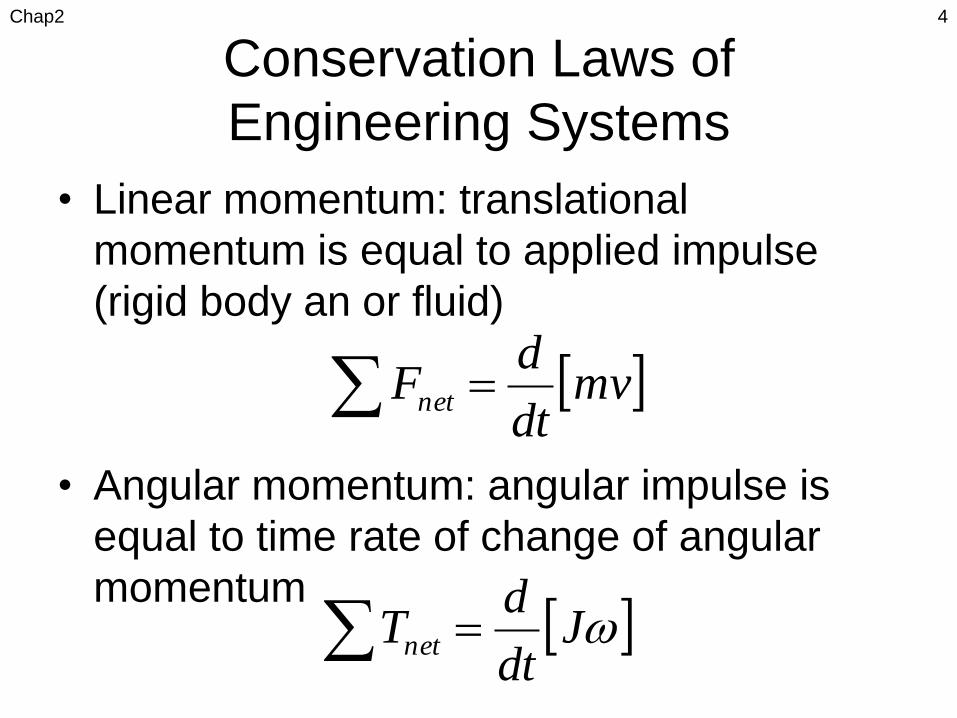
Conservation Laws of
Engineering Systems
• Linear momentum: translational
momentum is equal to applied impulse
(rigid body an or fluid)
• Angular momentum: angular impulse is
equal to time rate of change of angular
momentum
Chap2 4
mvdt
dFnet
Jdt
dTnet
Conservation Laws of
Engineering Systems
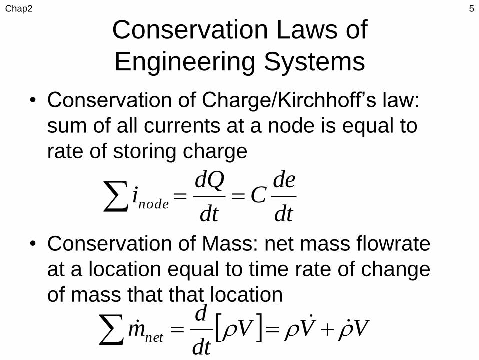
• Conservation of Charge/Kirchhoff’s law:
sum of all currents at a node is equal to
rate of storing charge
• Conservation of Mass: net mass flowrate
at a location equal to time rate of change
of mass that that location
Chap2 5
dt
deC
dt
dQinode
VVVdt
dmnet
Conservation Laws of
Engineering Systems
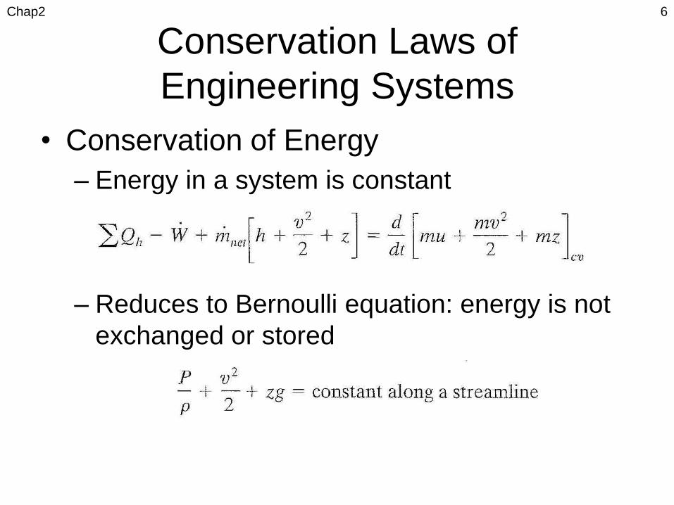
• Conservation of Energy
– Energy in a system is constant
– Reduces to Bernoulli equation: energy is not
exchanged or stored
Chap2 6

Review of Solution of
Differential Equations
Chap2 7
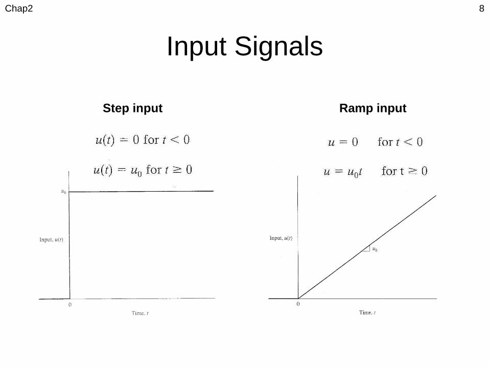
Input Signals
Chap2 8
Step input Ramp input
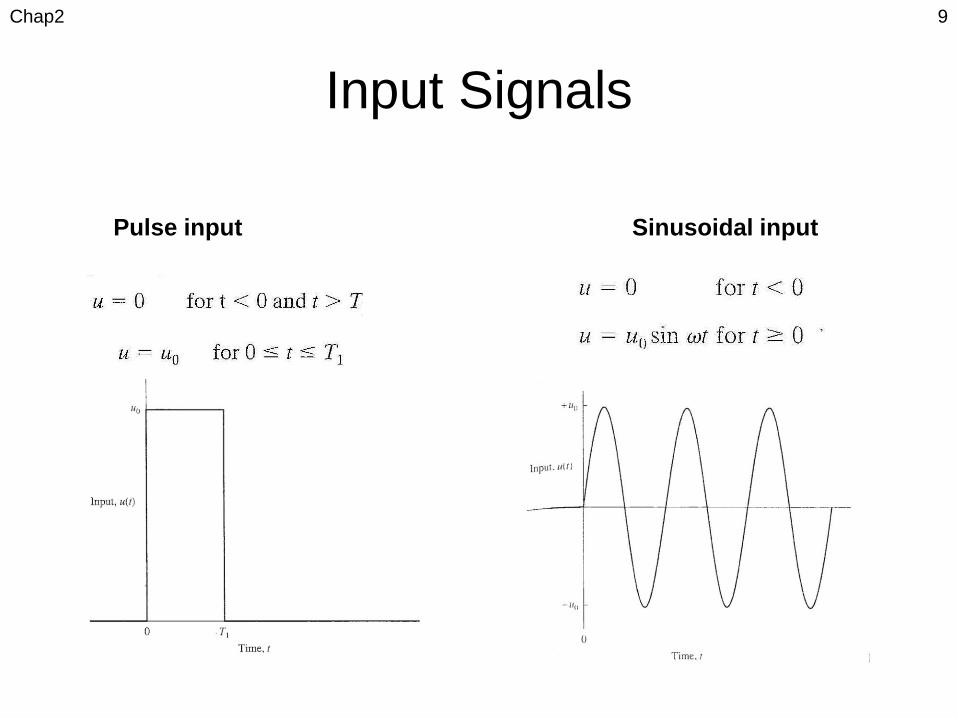
Input Signals
Chap2 9
Pulse input Sinusoidal input

Classical Differential EquationsChap2 10
)(]1[,,
.00
:1
1
01
001
tGuxDa
a
dt
dD
a
bGLet
aandaifstableisSystem
ubxadt
dxaOrder
oo
o
st
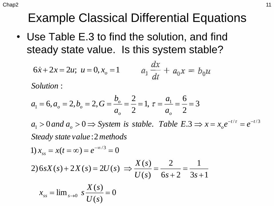
Example Classical Differential Equations
• Use Table E.3 to find the solution, and find
steady state value. Is this system stable?
Chap2 11
1,0;226 oxuuxx
0)(
)(lim
13
1
26
2
)(
)()(2)(2)(6)2
0)()1
2:
3..00
32
6,1
2
2,2,2,6
:
0
3/
3//
1
11
sU
sXsx
sssU
sXsUsXssX
etxx
methodsvaluestateSteady
eexxETablestableisSystemaanda
a
a
a
bGbaa
Solution
sss
ss
tt
oo
oo
ooo
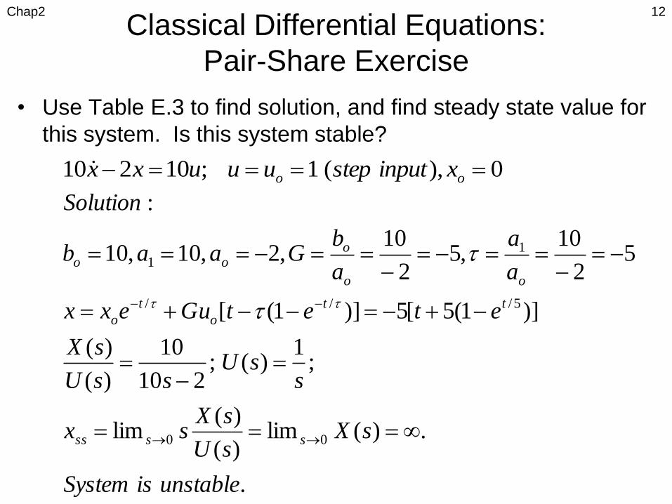
Classical Differential Equations:
Pair-Share Exercise
• Use Table E.3 to find solution, and find steady state value for
this system. Is this system stable?
Chap2 12
.
.)(lim)(
)(lim
;1
)(;210
10
)(
)(
)]1(5[5)]1([
52
10,5
2
10,2,10,10
:
00
5///
11
unstableisSystem
sXsU
sXsx
ssU
ssU
sX
etetGuexx
a
a
a
bGaab
Solution
ssss
tt
o
t
o
oo
ooo
0),(1;10210 oo xinputstepuuuxx
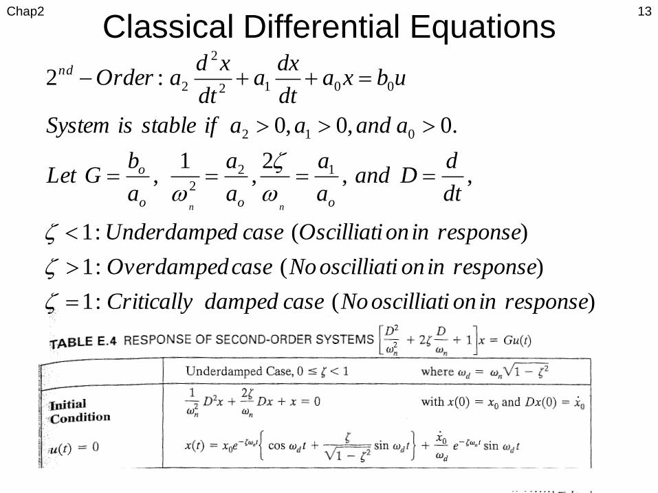
Classical Differential EquationsChap2 13
)(:1
)(:1
)(:1
,,2
,1
,
.0,0,0
:2
12
2
012
0012
2
2
responseinonoscilliatiNocasedampedCritically
responseinonoscilliatiNocaseOverdamped
responseinonOscilliaticasedUnderdampe
dt
dDand
a
a
a
a
a
bGLet
aandaaifstableisSystem
ubxadt
dxa
dt
xdaOrder
ooo
o
nd
nn
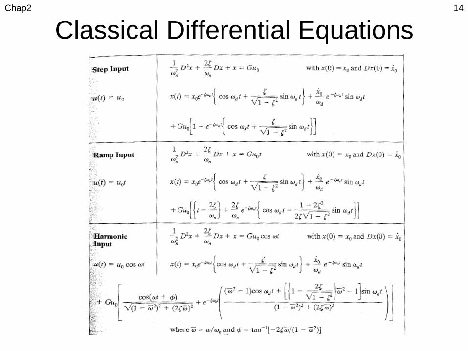
Chap2 14
Classical Differential Equations
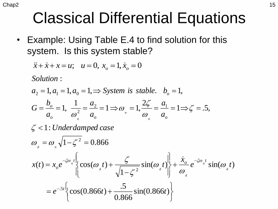
Classical Differential Equations
• Example: Using Table E.4 to find solution for this
system. Is this system stable?
Chap2 15
)866.0sin(866.0
5.)866.0cos(
)sin()sin(1
)cos()(
866.01
:1
,5.12
,111
,1
,1.,1,1,1
:
5.
2
2
12
2
012
tte
tex
ttextx
casedUnderdampe
a
a
a
a
a
bG
bstableisSystemaaa
Solution
t
tot
o
ooo
o
o
d
n
d
dd
n
nd
n
n
n
0,1,0; oo xxuuxxx

State Space Description
• State variables describe present configuration of
a system and can be used to determine future
response, given inputs and dynamic equations
• Number of state variables
– Should be as small as possible, but a minimum
number of state variables must be selected as
components of the state vector (sufficient to describe
completely the state of the system)
– Usually equal to order of system’s differential
equation or number of energy-storage elements
• Choice of state variables is not unique
Chap2 16
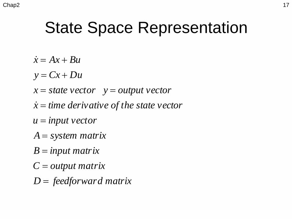
State Space Representation
Chap2 17
d matrixfeedforwarD
rixoutput matC
ixinput matrB
rixsystem matA
orinput vectu
ectorhe state vative of ttime derivx
toroutput vecor ystate vectx
DuCxy
BuAxx
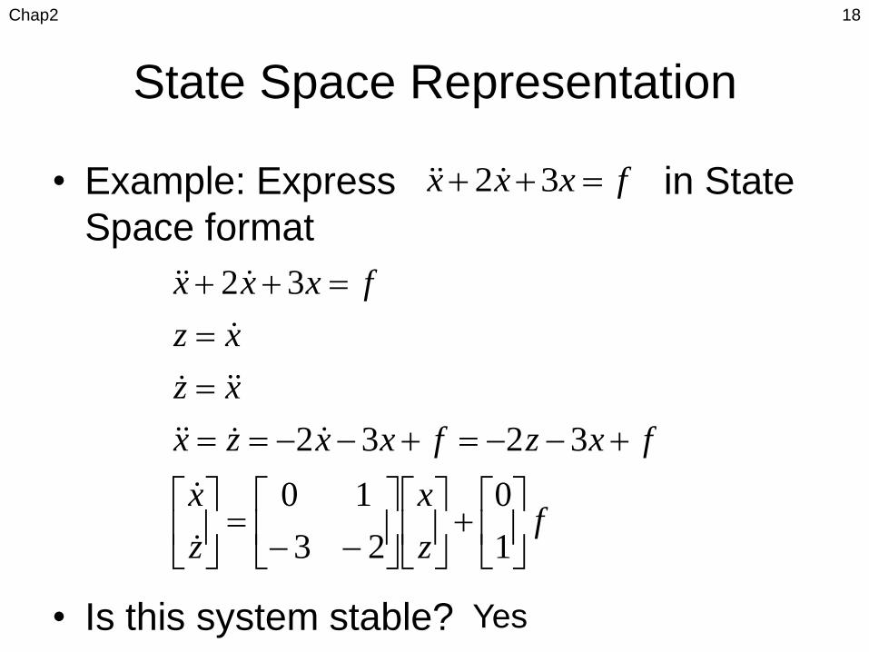
State Space Representation
• Example: Express in State
Space format
• Is this system stable?
Chap2 18
fz
x
z
x
fxzfxxzx
xz
xz
fxxx
1
0
23
10
3232
32
fxxx 32
Yes
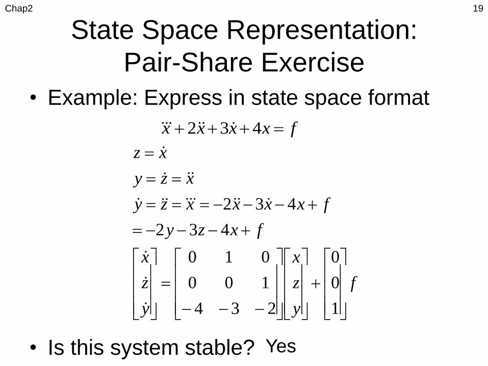
State Space Representation:
Pair-Share Exercise
• Example: Express in state space format
• Is this system stable?
Chap2 19
f
y
z
x
y
z
x
fxzy
fxxxxzy
xzy
xz
1
0
0
234
100
010
432
432
fxxxx 432
Yes
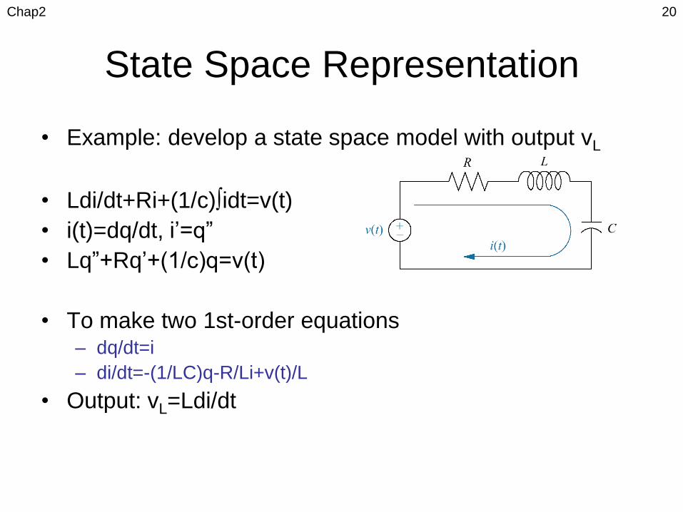
State Space Representation
• Example: develop a state space model with output vL
• Ldi/dt+Ri+(1/c)∫idt=v(t)
• i(t)=dq/dt, i’=q”
• Lq”+Rq’+(1/c)q=v(t)
• To make two 1st-order equations– dq/dt=i
– di/dt=-(1/LC)q-R/Li+v(t)/L
• Output: vL=Ldi/dt
Chap2 20
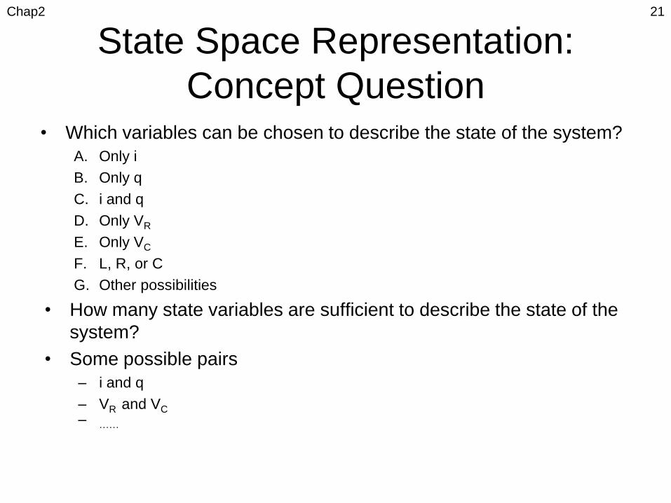
State Space Representation:
Concept Question• Which variables can be chosen to describe the state of the system?
A. Only i
B. Only q
C. i and q
D. Only VR
E. Only VC
F. L, R, or C
G. Other possibilities
• How many state variables are sufficient to describe the state of the
system?
• Some possible pairs
– i and q
– VR and VC
– ……
Chap2 21
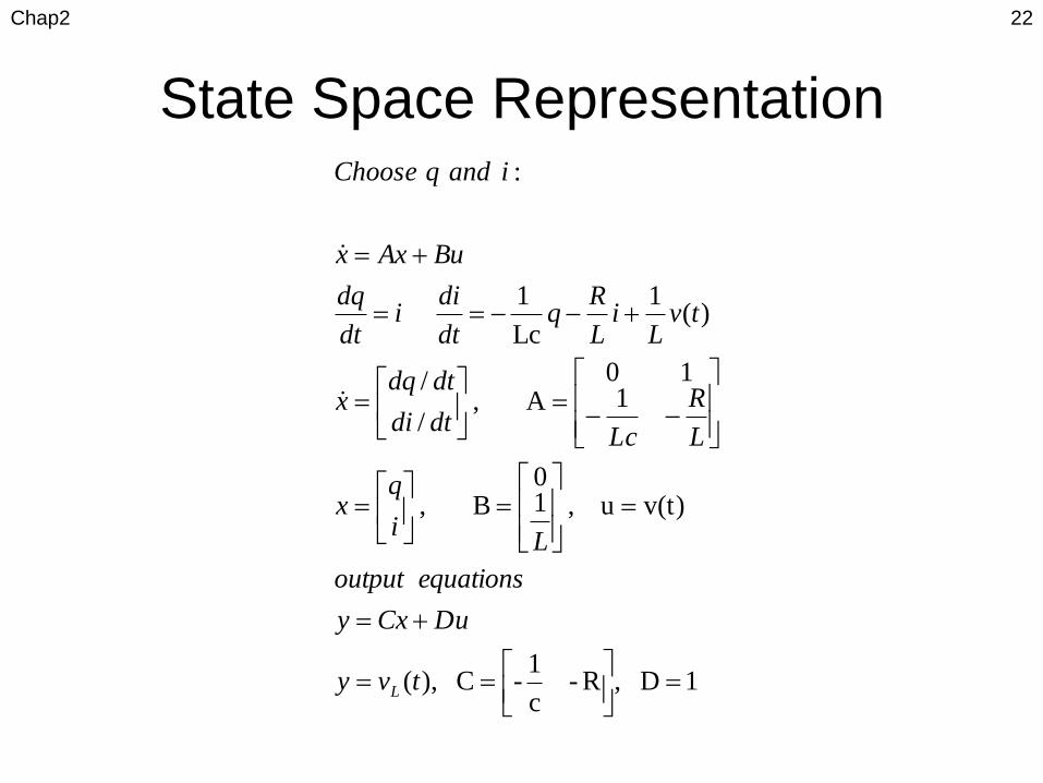
State Space Representation
Chap2 22
1D ,R-c
1-C ),(
v(t)u , 10
B ,
110
A , /
/
)(1
Lc
1
:
tvy
DuCxy
equationsoutput
Li
qx
L
R
Lcdtdi
dtdqx
tvL
iL
Rq
dt
dii
dt
dq
BuAxx
iandqChoose
L
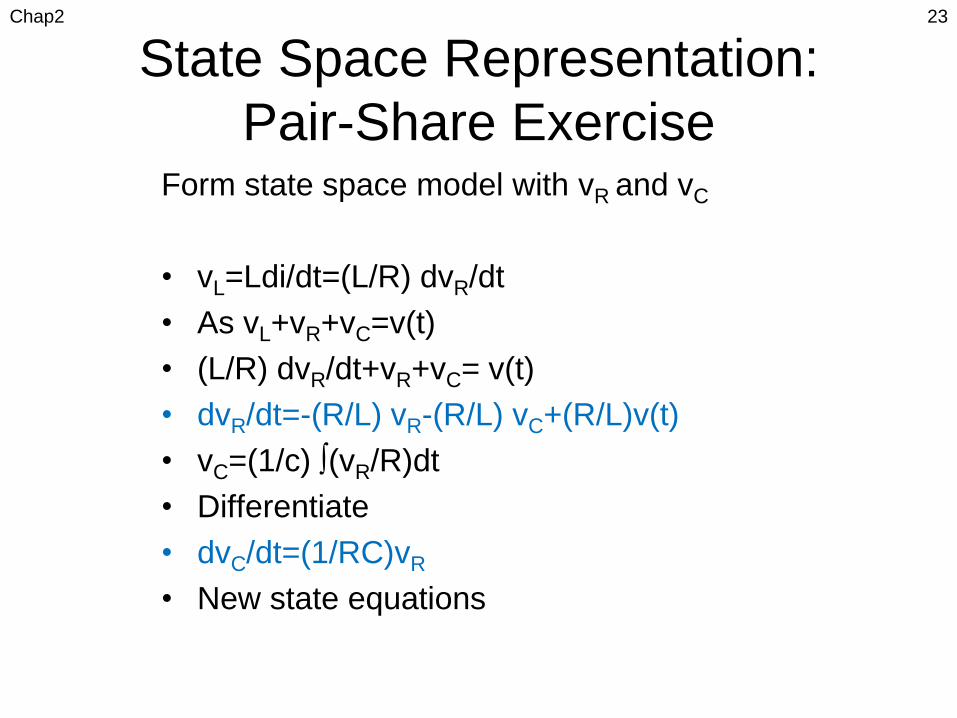
State Space Representation:
Pair-Share Exercise
Chap2 23
Form state space model with vR and vC
• vL=Ldi/dt=(L/R) dvR/dt
• As vL+vR+vC=v(t)
• (L/R) dvR/dt+vR+vC= v(t)
• dvR/dt=-(R/L) vR-(R/L) vC+(R/L)v(t)
• vC=(1/c) ∫(vR/R)dt
• Differentiate
• dvC/dt=(1/RC)vR
• New state equations
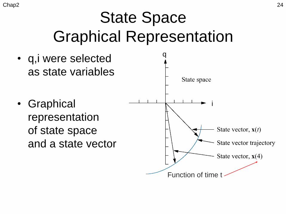
State Space
Graphical Representation
• q,i were selected
as state variables
• Graphical
representation
of state space
and a state vector
Chap2 24
Function of time t
q
i
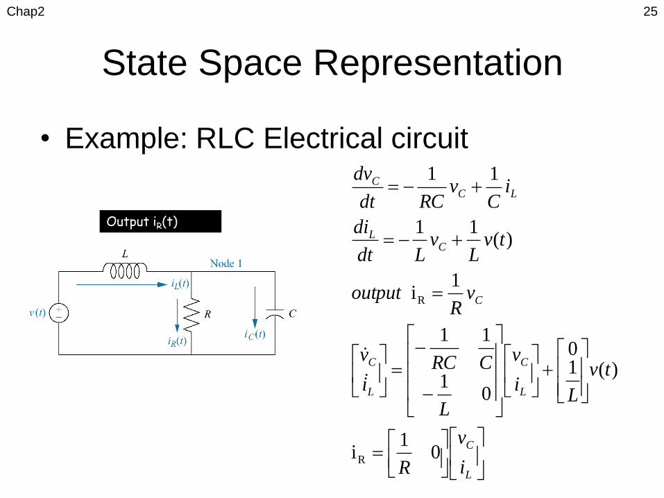
State Space Representation
• Example: RLC Electrical circuit
Chap2 25
L
C
L
C
L
C
C
CL
LCC
i
v
R
tv
Li
v
L
CRCi
v
vR
output
tvL
vLdt
di
iC
vRCdt
dv
01
i
)(10
01
11
1i
)(11
11
R
R
Output iR(t)
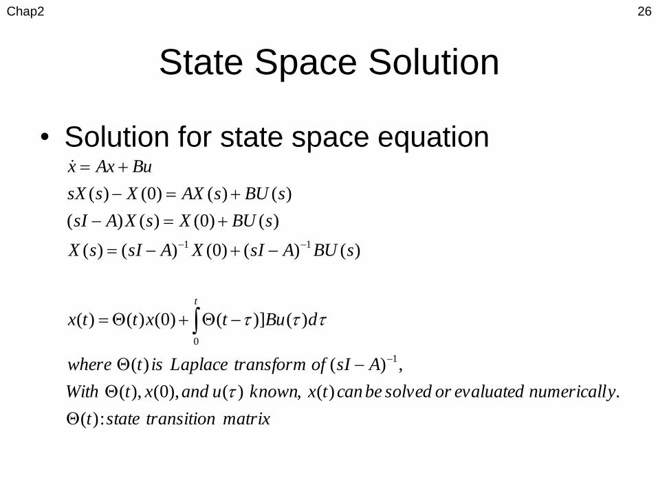
State Space Solution
• Solution for state space equation
Chap2 26
:)(
.)(,)(),0(),(
,)()(
)()]()0()()(
)()()0()()(
)()0()()(
)()()0()(
1
0
11
matrixtransitionstatet
ynumericallevaluatedorsolvedbecantxknownuandxtWith
AsIoftransformLaplaceistwhere
dButxttx
sBUAsIXAsIsX
sBUXsXAsI
sBUsAXXssX
BuAxx
t

State Space Solution
• Example
Chap2 27
tt
tt
tttt
tttt
ee
eexttx
eeee
eeeet
transformLaplaceinverseTake
ss
s
ss
ssss
s
s
s
sssAsI
uandxxx
2
2
22
22
1
1
22
2)0()()(
)2()22(
)()2()(
,
)2)(1()2)(1(
2
)2)(1(
1
)2)(1(
3
2
13
)2)(1(
1
32
10
10
01)(
.00
1)0(,
32
10
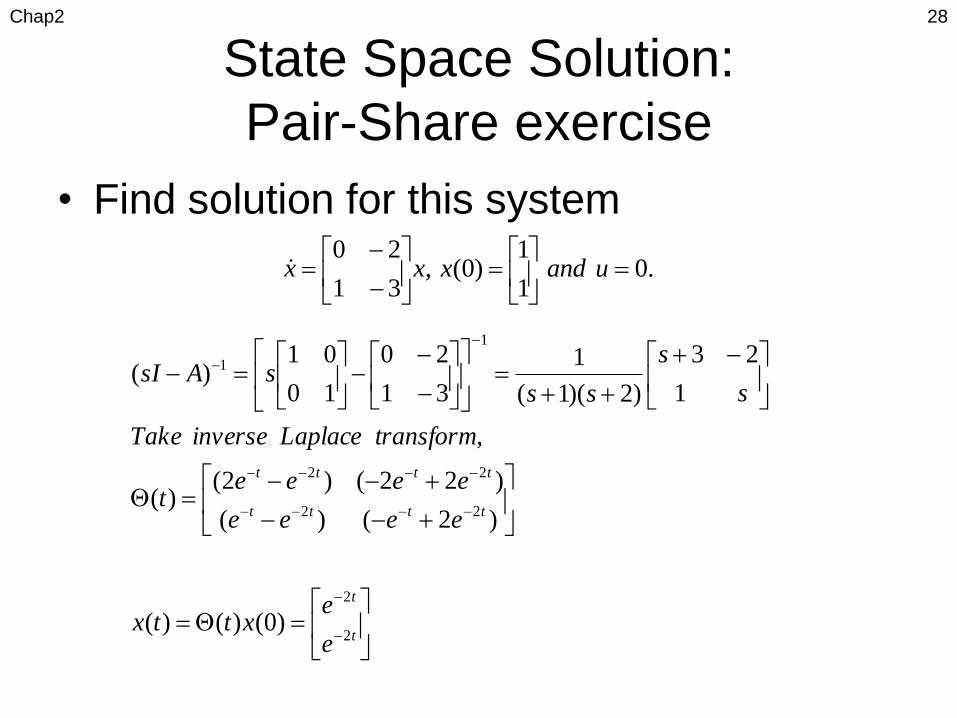
State Space Solution:
Pair-Share exercise
• Find solution for this system
Chap2 28
.01
1)0(,
31
20
uandxxx
t
t
tttt
tttt
e
exttx
eeee
eeeet
transformLaplaceinverseTake
s
s
sssAsI
2
2
22
22
1
1
)0()()(
)2()(
)22()2()(
,
1
23
)2)(1(
1
31
20
10
01)(
Engineering Systems
Similarity
Chap2 29
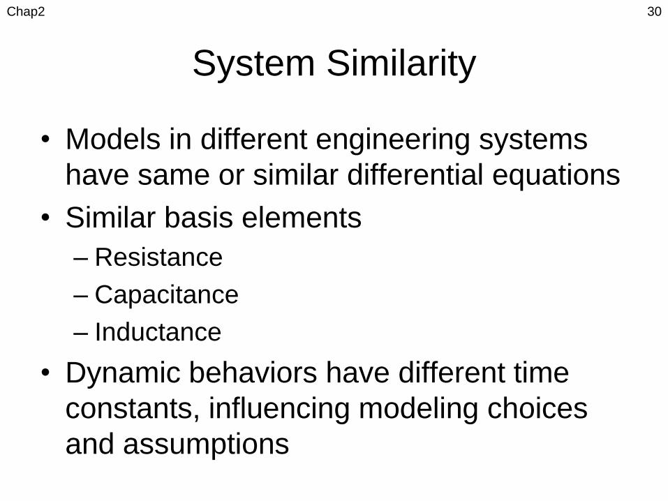
System Similarity
• Models in different engineering systems
have same or similar differential equations
• Similar basis elements
– Resistance
– Capacitance
– Inductance
• Dynamic behaviors have different time
constants, influencing modeling choices
and assumptions
Chap2 30
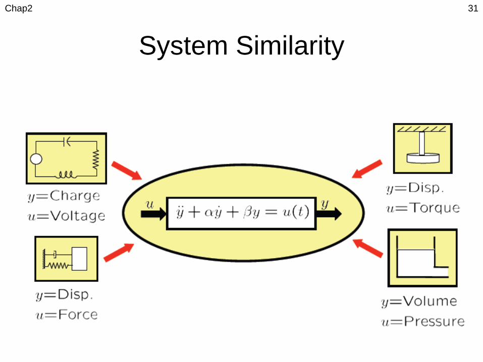
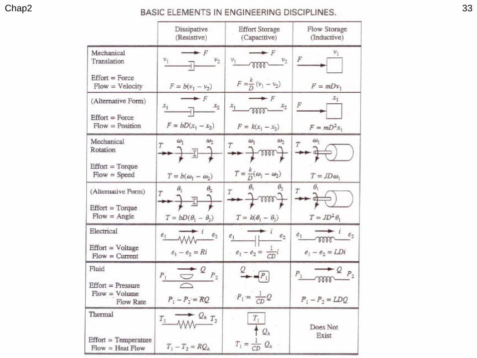
System Similarity
Chap2 31
Effort and Flow Variables
• Variables used for differential equations are
either effort or flow variables
– Effort variables: express effort placed on a
component, e.g., force, voltage
– Flow variables: express flow or time rate of change of
a system variable, e.g., velocity, current
• Impedance: is any transfer function between a
flow variable as input and effort variable as
output
– Effort = impedance x flow
– Impedance can be static (resistance) or dynamic
(capacitance/inductance)
Chap2 32
Chap2 33
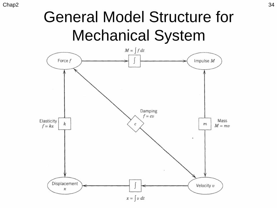
General Model Structure for
Mechanical System
Chap2 34

General Model Structure for
Electrical System
Chap2 35
Simulation with Matlab
Chap2 36
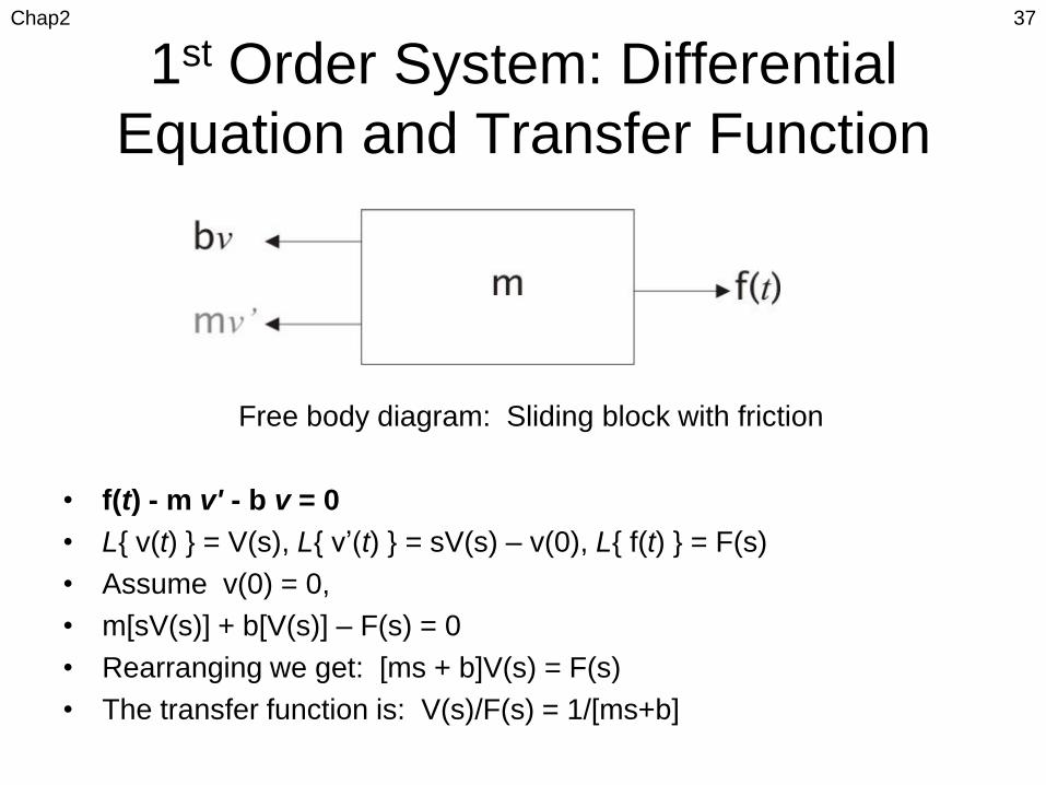
1st Order System: Differential
Equation and Transfer Function
Free body diagram: Sliding block with friction
• f(t) - m v' - b v = 0
• L{ v(t) } = V(s), L{ v’(t) } = sV(s) – v(0), L{ f(t) } = F(s)
• Assume v(0) = 0,
• m[sV(s)] + b[V(s)] – F(s) = 0
• Rearranging we get: [ms + b]V(s) = F(s)
• The transfer function is: V(s)/F(s) = 1/[ms+b]
Chap2 37
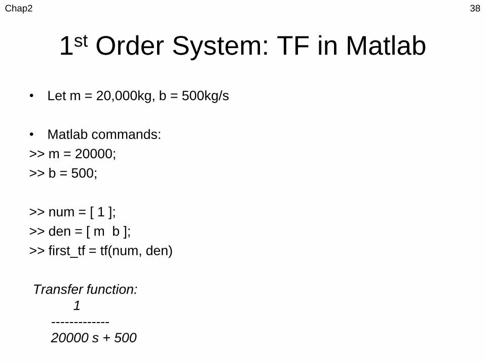
1st Order System: TF in Matlab
• Let m = 20,000kg, b = 500kg/s
• Matlab commands:
>> m = 20000;
>> b = 500;
>> num = [ 1 ];
>> den = [ m b ];
>> first_tf = tf(num, den)
Transfer function:
1
-------------
20000 s + 500
Chap2 38
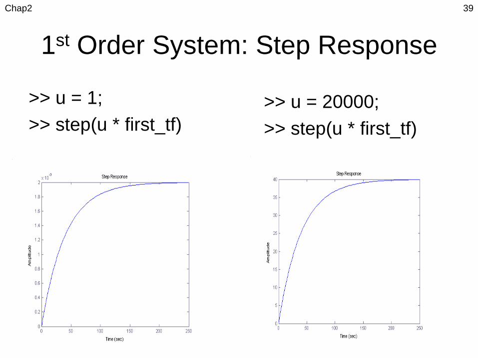
1st Order System: Step Response
>> u = 1;
>> step(u * first_tf)
Chap2 39
>> u = 20000;
>> step(u * first_tf)
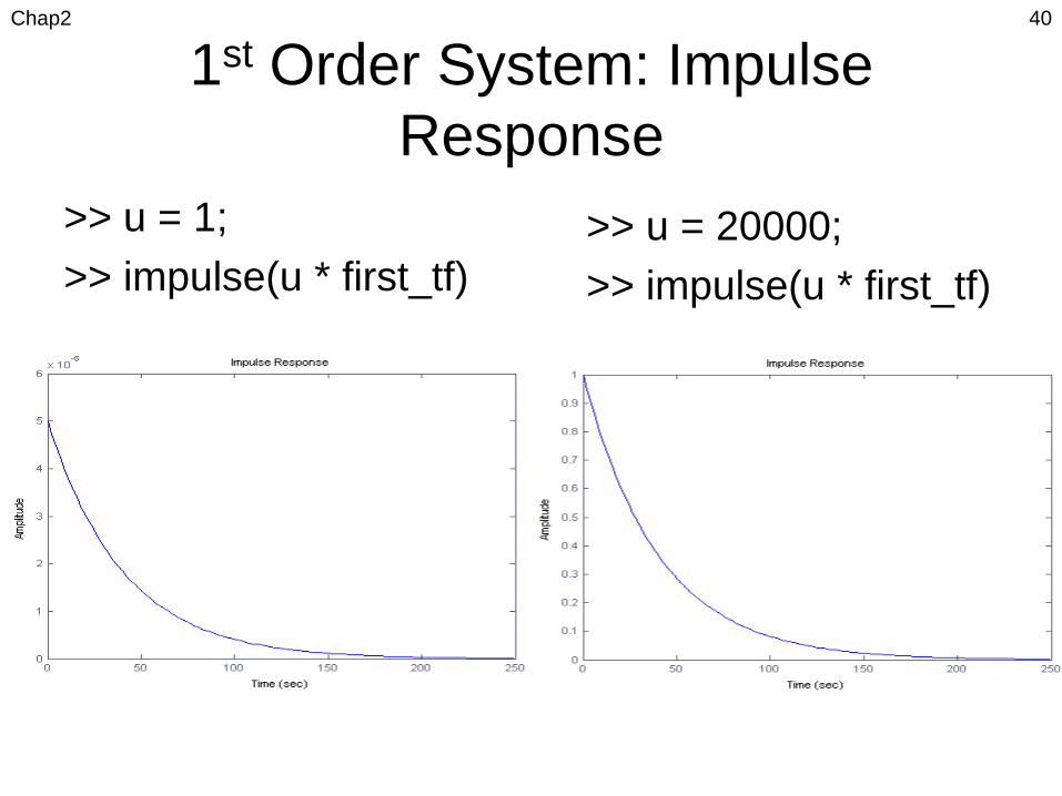
1st Order System: Impulse
Response
>> u = 1;
>> impulse(u * first_tf)
Chap2 40
>> u = 20000;
>> impulse(u * first_tf)
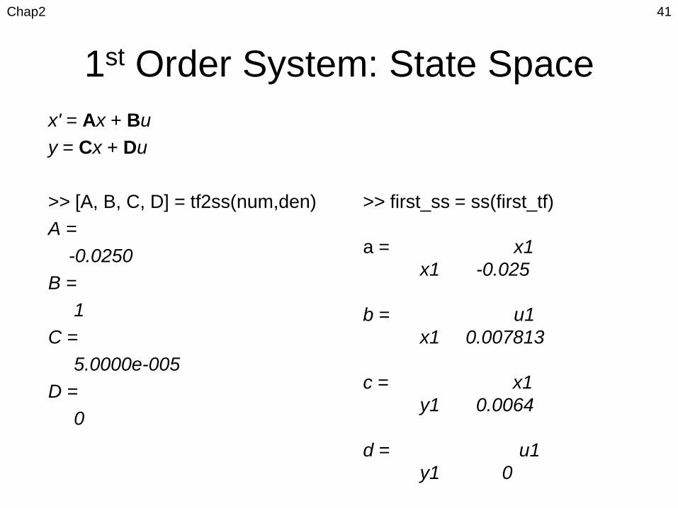
1st Order System: State Space
x' = Ax + Bu
y = Cx + Du
>> [A, B, C, D] = tf2ss(num,den)
A =
-0.0250
B =
1
C =
5.0000e-005
D =
0
Chap2 41
>> first_ss = ss(first_tf)
a = x1
x1 -0.025
b = u1
x1 0.007813
c = x1
y1 0.0064
d = u1
y1 0
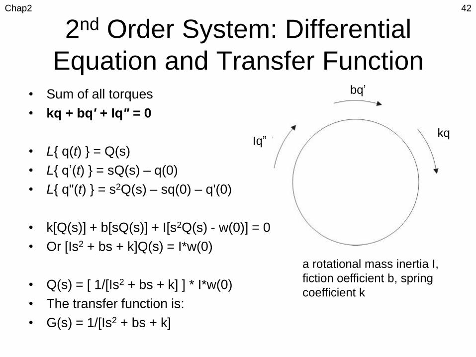
2nd Order System: Differential
Equation and Transfer Function• Sum of all torques
• kq + bq' + Iq" = 0
• L{ q(t) } = Q(s)
• L{ q’(t) } = sQ(s) – q(0)
• L{ q"(t) } = s2Q(s) – sq(0) – q'(0)
• k[Q(s)] + b[sQ(s)] + I[s2Q(s) - w(0)] = 0
• Or [Is2 + bs + k]Q(s) = I*w(0)
• Q(s) = [ 1/[Is2 + bs + k] ] * I*w(0)
• The transfer function is:
• G(s) = 1/[Is2 + bs + k]
Chap2 42
bq’
kqIq”
a rotational mass inertia I,
fiction oefficient b, spring
coefficient k
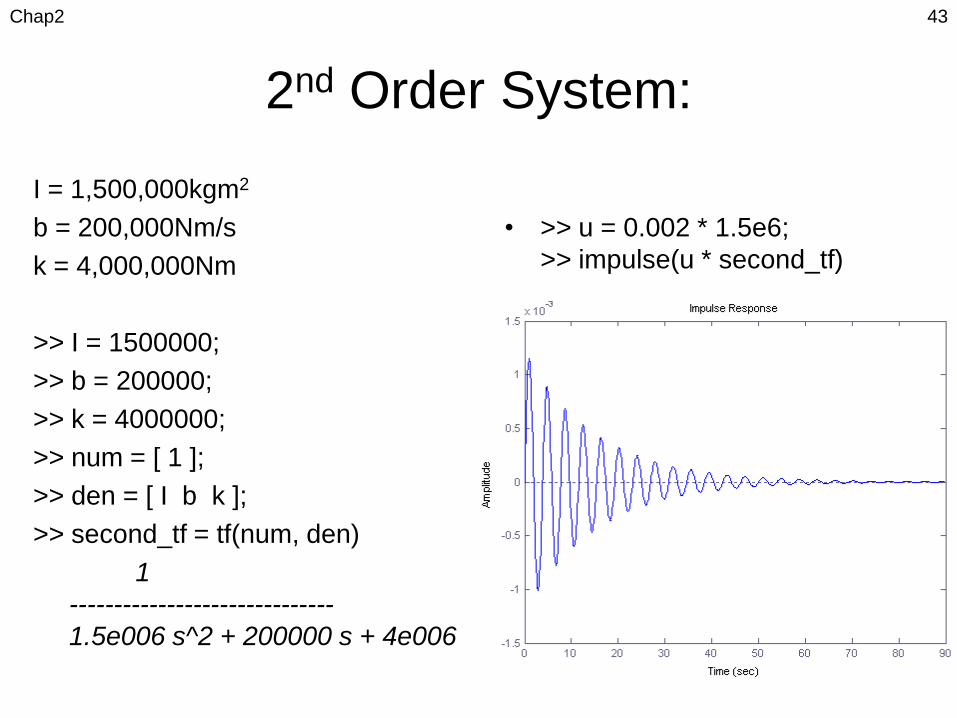
2nd Order System:
I = 1,500,000kgm2
b = 200,000Nm/s
k = 4,000,000Nm
>> I = 1500000;
>> b = 200000;
>> k = 4000000;
>> num = [ 1 ];
>> den = [ I b k ];
>> second_tf = tf(num, den)
1
------------------------------
1.5e006 s^2 + 200000 s + 4e006
Chap2 43
• >> u = 0.002 * 1.5e6;
>> impulse(u * second_tf)
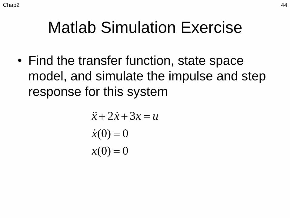
Matlab Simulation Exercise
• Find the transfer function, state space
model, and simulate the impulse and step
response for this system
Chap2 44
0)0(
0)0(
32
x
x
uxxx
Homework 2: chapter 2
• 2.14
• 2.15
• 2.24
• 2.25
Chap2 45
References
• Woods, R. L., and Lawrence, K., Modeling
and Simulation of Dynamic Systems,
Prentice Hall, 1997.
• Palm, W. J., Modeling, Analysis, and
Control of Dynamic Systems
• http://www.me.cmu.edu/ctms/index.html
Chap2 46


