45
Moderated Multiple Regression Class 22
| Date post: | 30-Dec-2015 |
| Category: |
Documents |
| Upload: | patricia-nash |
| View: | 216 times |
| Download: | 1 times |
Moderated Multiple Regression
Class 22

STATS TAKE HOME EXERCISE IS DUE THURSDAY DEC. 12
Regression Models
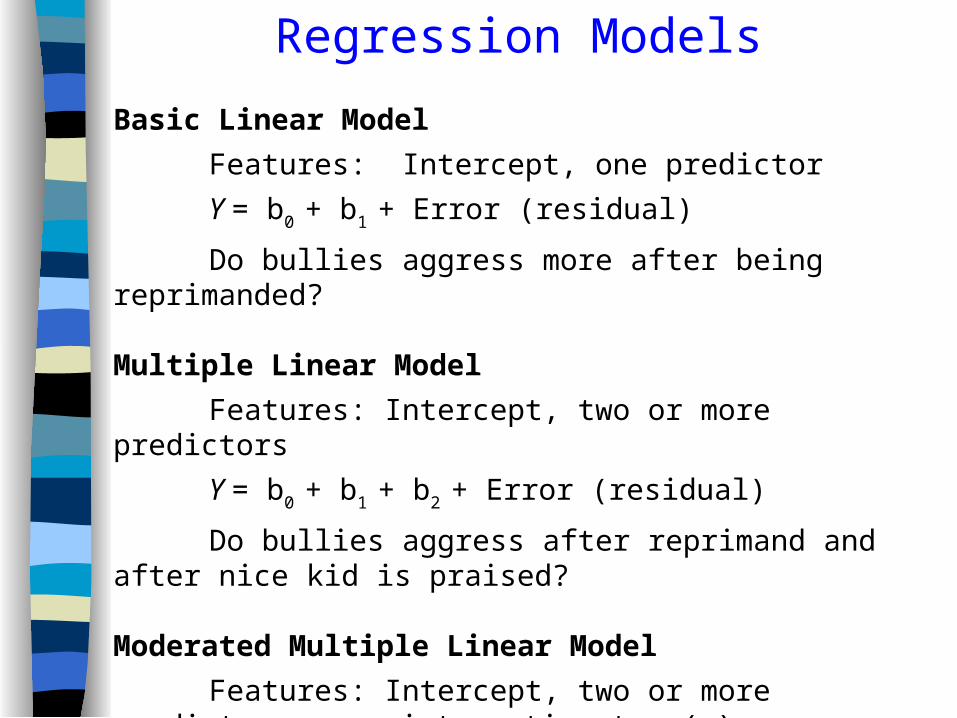
Basic Linear Model
Features: Intercept, one predictor
Y = b0 + b1 + Error (residual)
Do bullies aggress more after being reprimanded?
Multiple Linear Model
Features: Intercept, two or more predictors
Y = b0 + b1 + b2 + Error (residual)
Do bullies aggress after reprimand and after nice kid is praised?
Moderated Multiple Linear Model
Features: Intercept, two or more predictors, interaction term(s)
Y = b0 + b1 + b2 + b1b2 + Error (residual)
Aggress after reprimand, nice kid praised, and (reprimnd * praise)
THE KENT AND HERMAN DIALOGUE
A Moderated Multiple Regression Drama
With A Satisfactory Conclusion
Appropriate for All Audiences
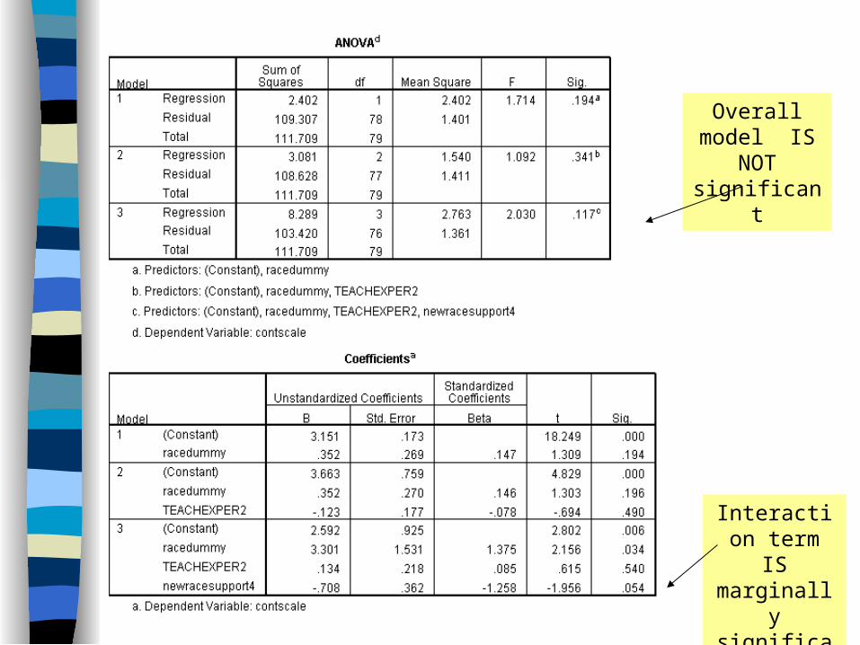
Overall model IS NOT
significant
Interaction term IS marginally
significant

Dear Dr. Aguinis, I am using your text in my graduate methods course. It is very clear and straightforward, which both my students and I appreciate.
A question came up that I thought you might be able to answer. If an MMR model produces a significant interaction, but the ANOVA F is not itself significant, is the significant interaction still a valid result? My impression is that the F of the overall model (as indicated by the ANOVA F and/or by the R-sqr. change) must be significant.
Thank you for your response, Kent Harber
Act 1, Scene 1: Kent contacts Herman regarding this vexing conundrum.
Kent, I believe you are referring to a test of a targeted interaction effect without looking at the overall (omnibus) effect. Please see pp. 134-135 of the book. Let me know if this does not answer your question and I will be delighted to follow up with you. Thanks for your kind words about my book! All the best, --Herman.
Act 1, scene 2: Herman replies!

Herman, thanks for getting back to me on this. Based on those pages of your text, it appears that the answer to my question is as follows:
If the omnibus F is itself not significant, then a significant interaction term within this non-significant model will itself not be interpretable.
Sadly (for some rather appealing interaction effects) this makes sense.
Again, very good of you to get back to me on this question. Best regards, Kent
Act 1, scene 3: Are simple effects doomed???
Kent, Before I give you an answer and to make sure I understand the question. What do you mean precisely by "the ANOVA F test"? Regards, --Herman.
Act 1, scene 4: Herman sustains the dramatic tension.

Kent, Thanks for the clarification.
Now, I understand your question perfectly.
An article by Bedeian and Mossholder (1994), J. of Management, addresses this question directly. The full citation is on page 177 of my book.
All the best, --Herman.
Act 1, scene 4: Herman drops the Big Clue

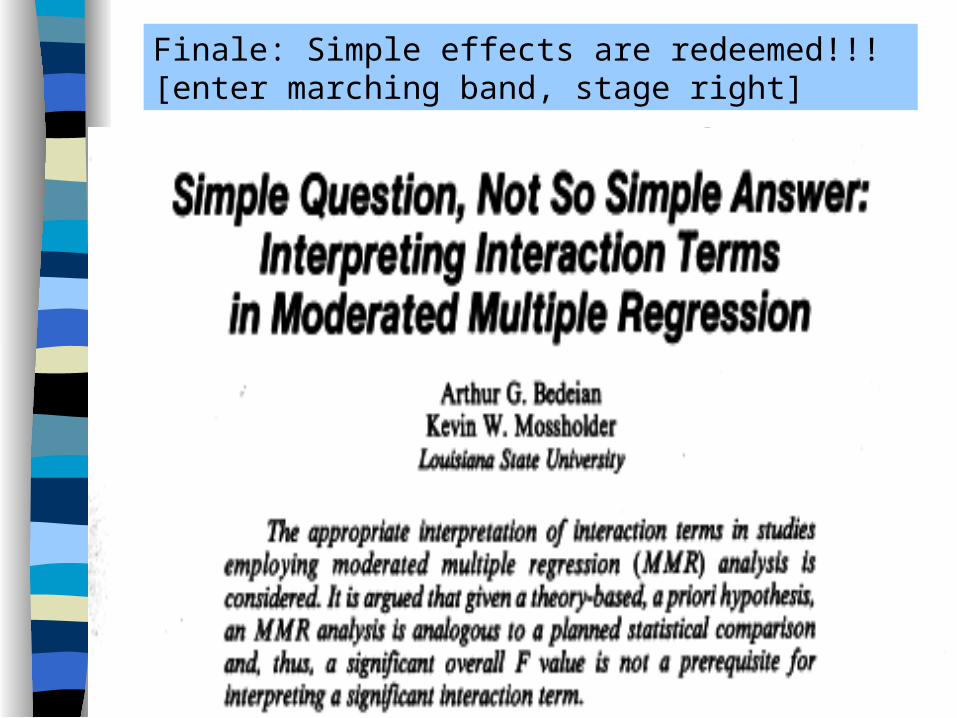
Finale: Simple effects are redeemed!!! [enter marching band, stage right]
Does Self Esteem Moderate the Use of Emotion as Information?
Harber, 2004, Personality and Social Psychology Bulletin, 31, 276-288
People use their emotions as information, especially when objective info. is lacking. Emotions are therefore persuasive messages from the self to the self. Are all people equally persuaded by their own emotions? Perhaps feeling good about oneself will affect whether to "believe" one's one emotions. Therefore, self-esteem should determine how much emotions affect judgment. Thus, when self-esteem is high, emotions should influence judgment more, and when self-esteem is low, emotions should influence judgments less.
Method: Studies 1 & 2
1. Collect self-esteem scores several weeks before experiment.
2. Subjects listen to series of 12 disturbing baby cries.
3. Subjects rate how much the baby is conveying distress through his cries, for each cry.
4. After rating all 12 cries, subjects indicate how upsetting it was for them to listen to the cries.
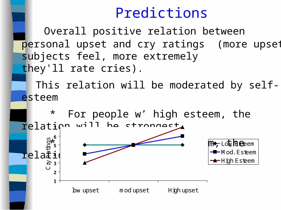
Predictions Overall positive relation between personal upset and cry
ratings (more upset subjects feel, more extremely they'll rate cries).
This relation will be moderated by self-esteem
* For people w’ high esteem, the relation will be strongest
* For people w’ low esteem, the relation will be weakest.
1
2
3
4
5
6
7
low upset mod upset High upset
Cry
Ra
ting
s
Low EsteemMod. EsteemHigh Esteem
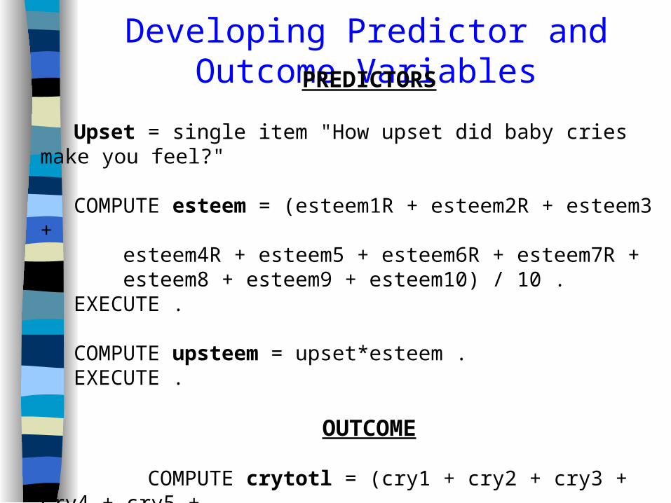
Developing Predictor and Outcome VariablesPREDICTORS
Upset = single item "How upset did baby cries make you feel?" COMPUTE esteem = (esteem1R + esteem2R + esteem3 + esteem4R + esteem5 + esteem6R + esteem7R + esteem8 + esteem9 + esteem10) / 10 .EXECUTE . COMPUTE upsteem = upset*esteem .EXECUTE .
OUTCOME
COMPUTE crytotl = (cry1 + cry2 + cry3 + cry4 + cry5 + cry6 + cry7 + cry8 + cry9 + cry10 + cry11 + cry12) / 12 . EXECUTE .
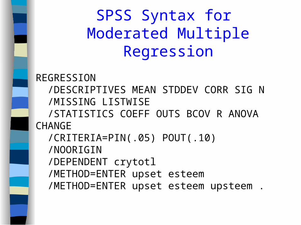
SPSS Syntax for Moderated Multiple Regression
REGRESSION /DESCRIPTIVES MEAN STDDEV CORR SIG N /MISSING LISTWISE /STATISTICS COEFF OUTS BCOV R ANOVA CHANGE /CRITERIA=PIN(.05) POUT(.10) /NOORIGIN /DEPENDENT crytotl /METHOD=ENTER upset esteem /METHOD=ENTER upset esteem upsteem .

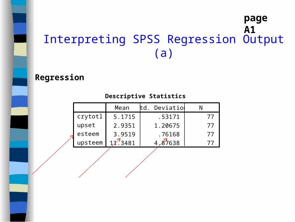
Interpreting SPSS Regression Output (a)
Regression
Descriptive Statistics
5.1715 .53171 77
2.9351 1.20675 77
3.9519 .76168 77
11.3481 4.87638 77
crytotl
upset
esteem
upsteem
Mean Std. Deviation N
page A1
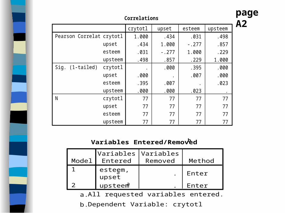
Correlations
1.000 .434 .031 .498
.434 1.000 -.277 .857
.031 -.277 1.000 .229
.498 .857 .229 1.000
. .000 .395 .000
.000 . .007 .000
.395 .007 . .023
.000 .000 .023 .
77 77 77 77
77 77 77 77
77 77 77 77
77 77 77 77
crytotl
upset
esteem
upsteem
crytotl
upset
esteem
upsteem
crytotl
upset
esteem
upsteem
Pearson Correlation
Sig. (1-tailed)
N
crytotl upset esteem upsteem
Variables Entered/Removedb
esteem,upset
a . Enter
upsteema . Enter
Model1
2
VariablesEntered
VariablesRemoved Method
All requested variables entered.a.
Dependent Variable: crytotlb.
page A2
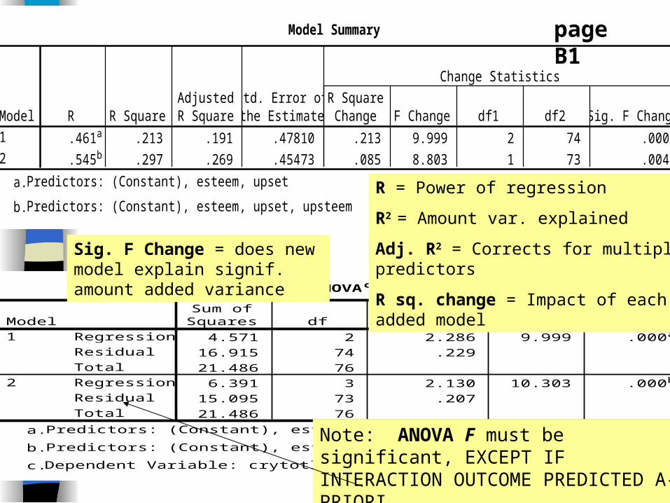
Model Summary
.461a .213 .191 .47810 .213 9.999 2 74 .000
.545b .297 .269 .45473 .085 8.803 1 73 .004
Model1
2
R R SquareAdjustedR Square
Std. Error ofthe Estimate
R SquareChange F Change df1 df2 Sig. F Change
Change Statistics
Predictors: (Constant), esteem, upseta.
Predictors: (Constant), esteem, upset, upsteemb.
page B1
ANOVAc
4.571 2 2.286 9.999 .000a
16.915 74 .229
21.486 76
6.391 3 2.130 10.303 .000b
15.095 73 .207
21.486 76
Regression
Residual
Total
Regression
Residual
Total
Model1
2
Sum ofSquares df Mean Square F Sig.
Predictors: (Constant), esteem, upseta.
Predictors: (Constant), esteem, upset, upsteemb.
Dependent Variable: crytotlc.
Note: ANOVA F must be significant, EXCEPT IF INTERACTION OUTCOME PREDICTED A-PRIORI
“Residual” = random error, NOT interaction
R = Power of regression
R2 = Amount var. explained
Adj. R2 = Corrects for multiple predictors
R sq. change = Impact of each added model
Sig. F Change = does new model explain signif. amount added variance
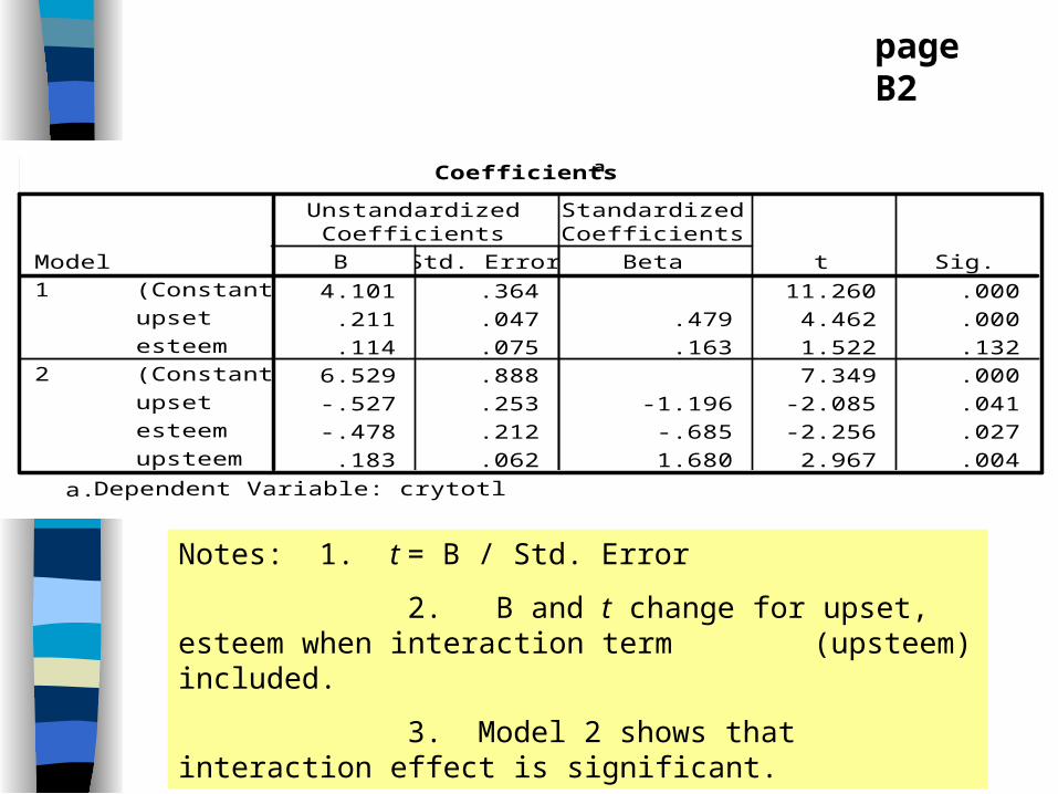
Coefficientsa
4.101 .364 11.260 .000
.211 .047 .479 4.462 .000
.114 .075 .163 1.522 .132
6.529 .888 7.349 .000
-.527 .253 -1.196 -2.085 .041
-.478 .212 -.685 -2.256 .027
.183 .062 1.680 2.967 .004
(Constant)
upset
esteem
(Constant)
upset
esteem
upsteem
Model1
2
B Std. Error
UnstandardizedCoefficients
Beta
StandardizedCoefficients
t Sig.
Dependent Variable: crytotla.
page B2
Notes: 1. t = B / Std. Error
2. B and t change for upset, esteem when interaction term (upsteem) included.
3. Model 2 shows that interaction effect is significant.
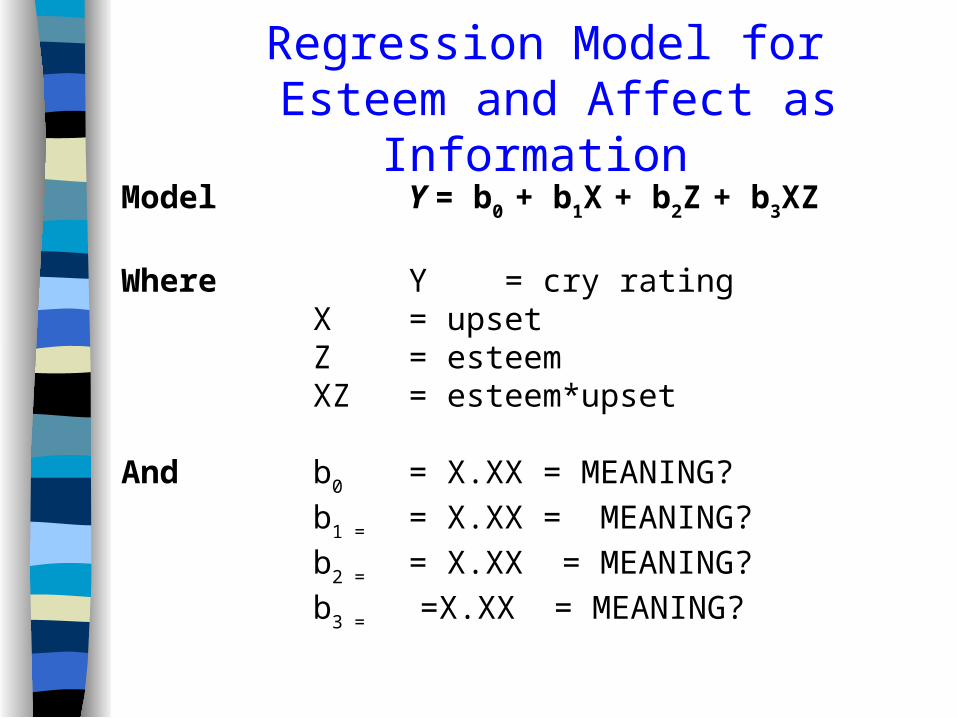
Regression Model for Esteem and Affect as Information
Model Y = b0 + b1X + b2Z + b3XZ Where Y = cry rating
X = upsetZ = esteemXZ = esteem*upset
And b0 = X.XX = MEANING?
b1 = = X.XX = MEANING?b2 = = X.XX = MEANING?b3 = =X.XX = MEANING?

Regression Model for Esteem and Affect as Information
Model: Y = b0 + b1X + b2Z + b3XZ Where Y = cry rating
X = upsetZ = esteemXZ = esteem*upset
And b0 = 6.53 = intercept (average score when
upset, esteem, upsetXexteem = 0)b1 = -0.57 = slope (influence) of upsetb2 = -0.48 = slope (influence) of esteemb3 = 0.18 = slope (influence) of upset X
esteem interaction
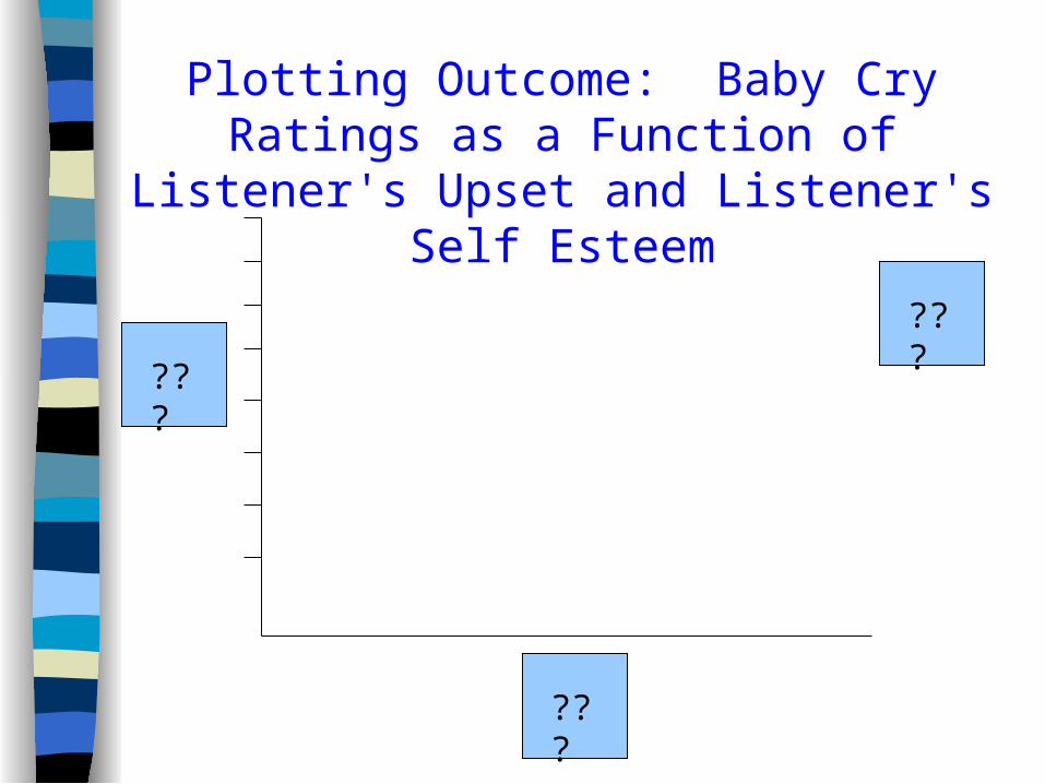
Plotting Outcome: Baby Cry Ratings as a Function of Listener's Upset and Listener's Self Esteem
???
???
???
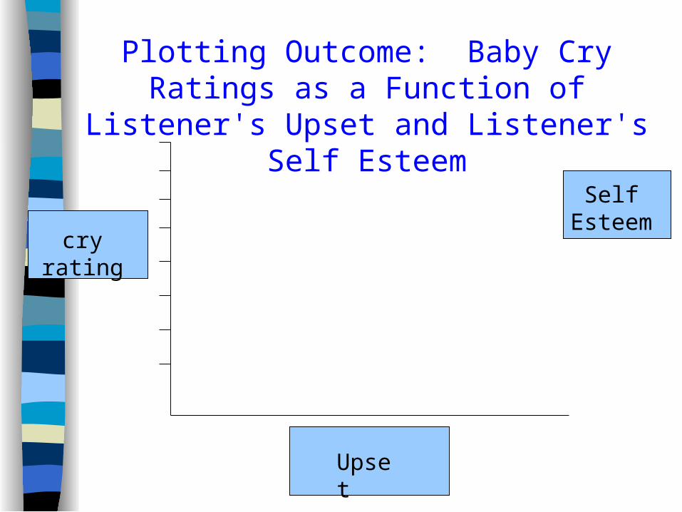
Plotting Outcome: Baby Cry Ratings as a Function of Listener's Upset and Listener's Self Esteem
cry rating
Upset
Self Esteem

Plotting Interactions with Two Continuous Variables
Y = b0 + b1X + b2Z + b3XZ
equals
Y = (b1 + b3Z)X + (b2Z + b0)
Y = (b1 + b3Z)X is simple slope of Y on X at Z.
Means "the effect X has on Y, conditioned by the interactive contribution of Z." Thus, when Z is one value, the X slope takes one shape, when Z is another value, the X slope takes other shape.
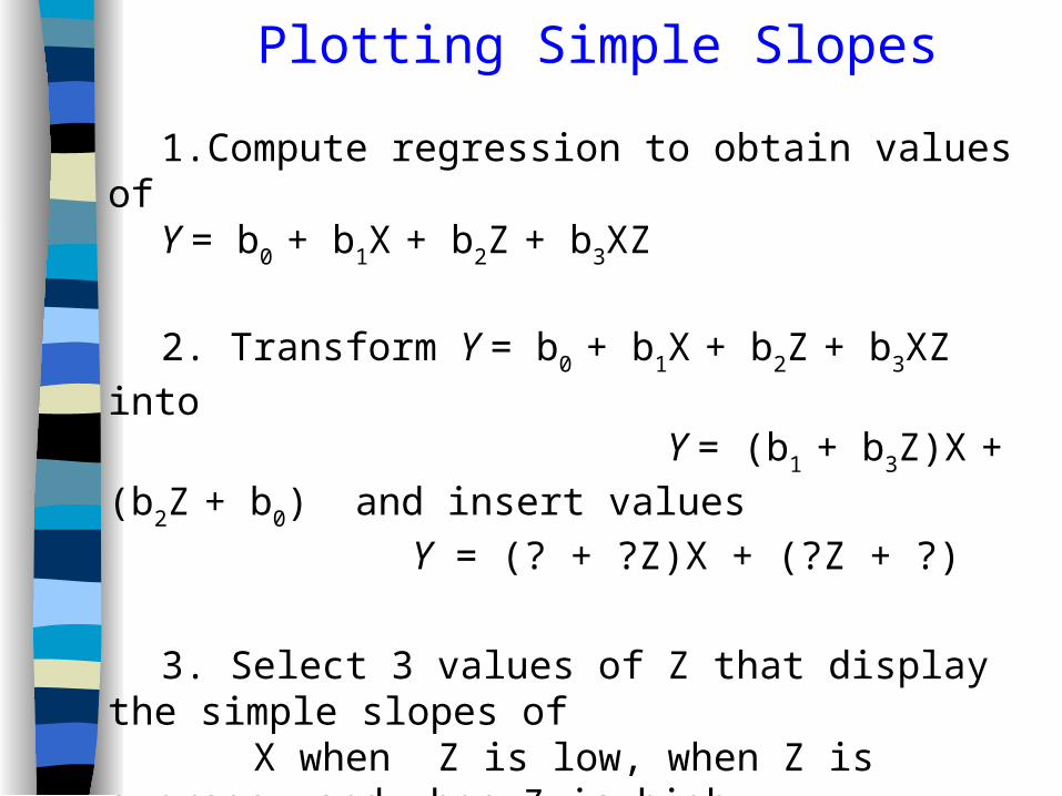
Plotting Simple Slopes
1.Compute regression to obtain values of Y = b0 + b1X + b2Z + b3XZ
2. Transform Y = b0 + b1X + b2Z + b3XZ into Y = (b1 + b3Z)X + (b2Z + b0) and insert values
Y = (? + ?Z)X + (?Z + ?)
3. Select 3 values of Z that display the simple slopes of X when Z is low, when Z is average, and when Z is high.
Standard practice: Z at one SD above the mean = ZH
Z at the mean = ZM
Z at one SD below the mean = ZL
Interpreting SPSS Regression Output (a)
Regression
Descriptive Statistics
5.1715 .53171 77
2.9351 1.20675 77
3.9519 .76168 77
11.3481 4.87638 77
crytotl
upset
esteem
upsteem
Mean Std. Deviation N
page A1
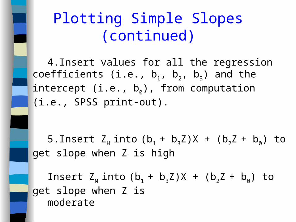
4.Insert values for all the regression coefficients (i.e., b1, b2, b3) and the intercept (i.e., b0), from computation (i.e., SPSS print-out).
5.Insert ZH into (b1 + b3Z)X + (b2Z + b0) to get slope when Z is high
Insert ZM into (b1 + b3Z)X + (b2Z + b0) to get slope when Z ismoderate
Insert ZL into (b1 + b3Z)X + (b2Z + b0) to get slope when Z is low
Plotting Simple Slopes(continued)

Example of Plotting Baby Cry Study, Part IY (cry rating) = b0 (rating when all predictors = zero)
+ b1X (effect of upset) + b2Z (effect of esteem) + b3XZ (effect of upset X esteem interaction).
Y = 6.53 + -.53X -.48Z + .18XZ.
Y = (b1 + b3Z)X + (b2Z + b0) [conversion for simple slopes] Y = (-.53 + .18Z)X + (-.48Z + 6.53)
Compute ZH, ZM, ZL via “Frequencies" for esteem, 3.95 = mean, .76 = SD
ZH, = (3.95 + .76) = 4.71 ZM = (3.95 + 0) = 3.95
ZL = (3.95 - .76) = 3.19
Slope at ZH = (-.53 + .18 * 4.71)X + ([-.48 * 4.71] + 6.53) = .32X + 4.27
Slope at ZM = (-.53 + .18 * 3.95)X + ([-.48 * 3.95] + 6.53) = .18X + 4.64
Slope at ZL = (-.53 + .18 * 3.19)X + ([-.48 * 3.19] + 6.53) = .04X + 4.99

Example of Plotting, Baby Cry Study, Part II1. Compute mean and SD of main predictor ("X") i.e., Upset
Upset mean = 2.94, SD = 1.21
2. Select values on the X axis displaying main predictor, e.g. upset at:
Low upset = 1 SD below mean` = 2.94 – 1.21 = 1.73Medium upset = mean = 2.94 – 0.00 = 2.94High upset = 1SD above mean = 2.94 + 1.21 = 4.15
3. Plug these values into ZH, ZM, ZL simple slope equations
Simple Slope
Formula Low Upset(X = 1.73)
Medium Upset(X = 2.94)
High Upset(X = 4.15)
ZH .32X + 4.28 4.83 5.22 5.61
ZM .18X + 4.64 4.95 5.17 5.38
ZL .04X + 4.99 5.06 5.11 5.16
4. Plot values into graph

Graph Displaying Simple Slopes
4.6
5
5.4
5.8
Mild Upset Mod. Upset Extreme Upset
Participants' Level of Upset
Baby
Cry
Rat
ings
High EsteemMed. EsteemLow Esteem

Are the Simple Slopes Significant? Question: Do the slopes of each of the simple effects lines (ZH, ZM, ZL) significantly differ from zero? Procedure to test, using as an example ZH (the slope when esteem is high): 1. Transform Z to Zcvh (CV = conditional value) by subtracting ZH from Z.
Zcvh = Z - ZH = Z – 4.71 Conduct this transformation in SPSS as: COMPUTE esthigh = esteem - 4.71.
2. Create new interaction term specific to Zcvh, i.e., (X* Zcvh)
COMPUTE upesthi = upset*esthigh . 3. Run regression, using same X as before, but substituting
Zcvh for Z, and X* Zcvh for XZ
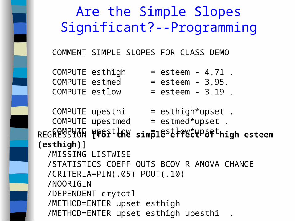
Are the Simple Slopes Significant?--Programming COMMENT SIMPLE SLOPES FOR CLASS DEMO COMPUTE esthigh = esteem - 4.71 . COMPUTE estmed = esteem - 3.95. COMPUTE estlow = esteem - 3.19 . COMPUTE upesthi = esthigh*upset . COMPUTE upestmed = estmed*upset . COMPUTE upestlow = estlow*upset .
REGRESSION [for the simple effect of high esteem (esthigh)] /MISSING LISTWISE /STATISTICS COEFF OUTS BCOV R ANOVA CHANGE /CRITERIA=PIN(.05) POUT(.10) /NOORIGIN /DEPENDENT crytotl /METHOD=ENTER upset esthigh /METHOD=ENTER upset esthigh upesthi .
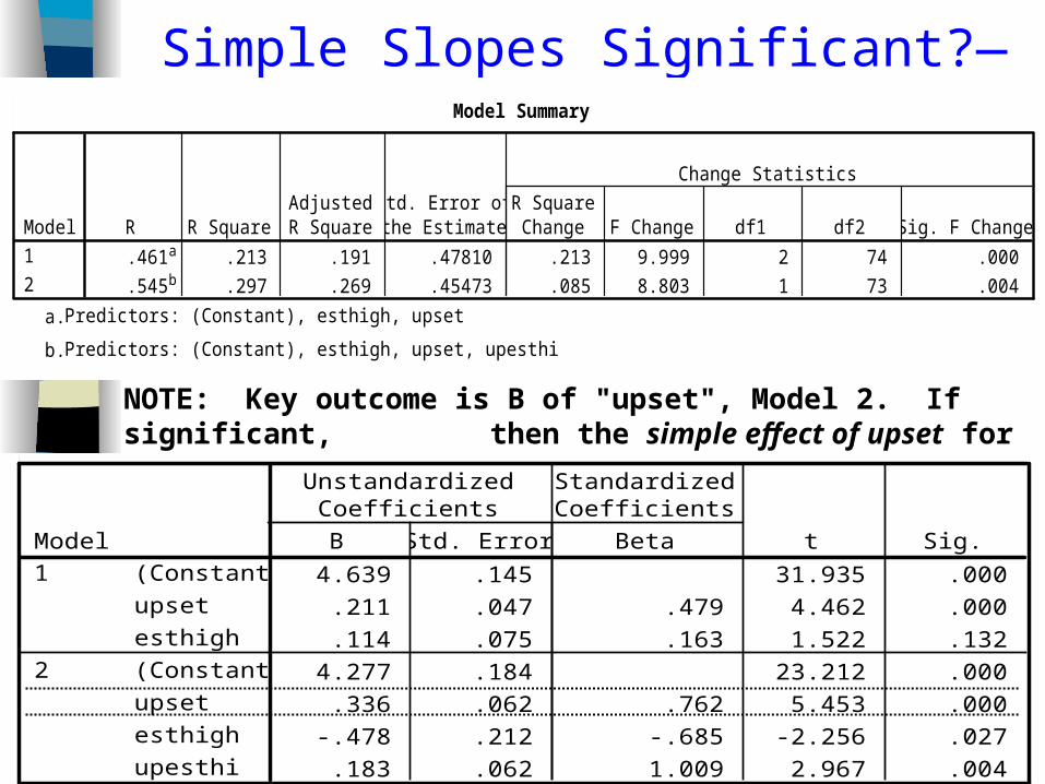
Simple Slopes Significant?—Results
Regression Model Summary
.461a .213 .191 .47810 .213 9.999 2 74 .000
.545b .297 .269 .45473 .085 8.803 1 73 .004
Model1
2
R R SquareAdjustedR Square
Std. Error ofthe Estimate
R SquareChange F Change df1 df2 Sig. F Change
Change Statistics
Predictors: (Constant), esthigh, upseta.
Predictors: (Constant), esthigh, upset, upesthib.
NOTE: Key outcome is B of "upset", Model 2. If significant, then the simple effect of upset for the high esteem slope is signif.Coefficientsa
4.639 .145 31.935 .000
.211 .047 .479 4.462 .000
.114 .075 .163 1.522 .132
4.277 .184 23.212 .000
.336 .062 .762 5.453 .000
-.478 .212 -.685 -2.256 .027
.183 .062 1.009 2.967 .004
(Constant)
upset
esthigh
(Constant)
upset
esthigh
upesthi
Model1
2
B Std. Error
UnstandardizedCoefficients
Beta
StandardizedCoefficients
t Sig.
Dependent Variable: crytotla.
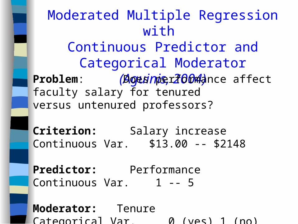
Moderated Multiple Regression with Continuous Predictor and Categorical Moderator
(Aguinis, 2004)
Problem: Does performance affect faculty salary for tenured versus untenured professors? Criterion: Salary increase Continuous Var. $13.00 -- $2148 Predictor: Performance Continuous Var. 1 -- 5 Moderator: Tenure Categorical Var. 0 (yes) 1 (no)
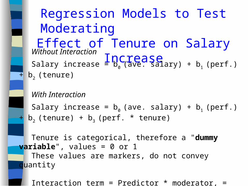
Regression Models to Test Moderating Effect of Tenure on Salary Increase
Without Interaction
Salary increase = b0 (ave. salary) + b1 (perf.) + b2 (tenure) With Interaction
Salary increase = b0 (ave. salary) + b1 (perf.) + b2 (tenure) + b3 (perf. * tenure) Tenure is categorical, therefore a "dummy variable", values = 0 or 1 These values are markers, do not convey quantity Interaction term = Predictor * moderator, = perf. * tenure. That simple. Conduct regression, plotting, simple slopes analyses same as when predictor and moderator are both continuous variables.

Centering Data
Centering data is done to standardize it. Aiken and West recommend doing it in all cases.
* Makes zero score meaningful* Has other benefits
Aguinas recommends doing it in some cases.* Sometimes uncentered scores are meaningful
Procedure
upset M = 2.94, SD = 1.19; esteem M = 3.94, SD = 0.75
COMPUTE upcntr = upset – 2.94.COMPUTE estcntr = esteem = 3.94
upcntr M = 0, SD = 1.19; esteem M = 0, SD = 0.75 Centering may affect the slopes of predictor and moderator, BUTit does not affect the interaction term.

THE KENT AND HERMAN DIALOGUE
A Moderated Multiple Regression Drama
With A Satisfactory Conclusion
Appropriate for All Audiences

Overall model IS NOT
significant
Interaction term IS marginally
significant
Dear Dr. Aguinis, I am using your text in my graduate methods course. It is very clear and straightforward, which both my students and I appreciate.
A question came up that I thought you might be able to answer. If an MMR model produces a significant interaction, but the ANOVA F is not itself significant, is the significant interaction still a valid result? My impression is that the F of the overall model (as indicated by the ANOVA F and/or by the R-sqr. change) must be significant.
Thank you for your response, Kent Harber
Act 1, Scene 1: Kent contacts Herman regarding this vexing conundrum.

Kent, I believe you are referring to a test of a targeted interaction effect without looking at the overall (omnibus) effect. Please see pp. 134-135 of the book. Let me know if this does not answer your question and I will be delighted to follow up with you. Thanks for your kind words about my book! All the best, --Herman.
Act 1, scene 2: Herman replies!
Herman, thanks for getting back to me on this. Based on those pages of your text, it appears that the answer to my question is as follows:
If the omnibus F is itself not significant, then a significant interaction term within this non-significant model will itself not be interpretable.
Sadly (for some rather appealing interaction effects) this makes sense.
Again, very good of you to get back to me on this question. Best regards, Kent
Act 1, scene 3: Are simple effects doomed???

Kent, Before I give you an answer and to make sure I understand the question. What do you mean precisely by "the ANOVA F test"? Regards, --Herman.
Act 1, scene 4: Herman sustains the dramatic tension.
Kent, Thanks for the clarification.
Now, I understand your question perfectly.
An article by Bedeian and Mossholder (1994), J. of Management, addresses this question directly. The full citation is on page 177 of my book.
All the best, --Herman.
Act 1, scene 4: Herman drops the Big Clue
Finale: Simple effects are redeemed!!! [enter marching band, stage right]


![Arthritis Research UK Epidemiology Unit University of ...personalpages.manchester.ac.uk/staff/mark.lunt/stats/11_Stata_2/...Other Graph Types twoway lfit[ci] Linear regression fit](https://static.documents.pub/doc/80x56/5aafdfdb7f8b9a22118dc053/arthritis-research-uk-epidemiology-unit-university-of-graph-types-twoway-lfitci.jpg)

