347
MODERN ALGEBRA WITH APPLICATIONS

MODERN ALGEBRAWITH APPLICATIONS
PURE AND APPLIED MATHEMATICS
A Wiley-Interscience Series of Texts, Monograph, and Tracts
Founded by RICHARD COURANTEditors: MYRON B. ALLEN III, DAVID A. COX, PETER LAXEditors Emeriti: PETER HILTON, HARRY HOCHSTADT, JOHN TOLAND
A complete list of the titles in this series appears at the end of this volume.

MODERN ALGEBRAWITH APPLICATIONS
Second Edition
WILLIAM J. GILBERTUniversity of WaterlooDepartment of Pure MathematicsWaterloo, Ontario, Canada
W. KEITH NICHOLSONUniversity of CalgaryDepartment of Mathematics and StatisticsCalgary, Alberta, Canada
A JOHN WILEY & SONS, INC., PUBLICATION

Cover: Still image from the applet KaleidoHedron, Copyright 2000 by Greg Egan, from hiswebsite http://www.netspace.net.au/∼gregegan/. The pattern has the symmetry of the icosahedralgroup.
Copyright 2004 by John Wiley & Sons, Inc. All rights reserved.
Published by John Wiley & Sons, Inc., Hoboken, New Jersey.Published simultaneously in Canada.
No part of this publication may be reproduced, stored in a retrieval system, or transmitted in anyform or by any means, electronic, mechanical, photocopying, recording, scanning, or otherwise,except as permitted under Section 107 or 108 of the 1976 United States Copyright Act, withouteither the prior written permission of the Publisher, or authorization through payment of theappropriate per-copy fee to the Copyright Clearance Center, Inc., 222 Rosewood Drive, Danvers,MA 01923, 978-750-8400, fax 978-750-4470, or on the web at www.copyright.com. Requests tothe Publisher for permission should be addressed to the Permissions Department, John Wiley &Sons, Inc., 111 River Street, Hoboken, NJ 07030, (201) 748-6011, fax (201) 748-6008, e-mail:[email protected].
Limit of Liability/Disclaimer of Warranty: While the publisher and author have used their bestefforts in preparing this book, they make no representations or warranties with respect to theaccuracy or completeness of the contents of this book and specifically disclaim any impliedwarranties of merchantability or fitness for a particular purpose. No warranty may be created orextended by sales representatives or written sales materials. The advice and strategies containedherein may not be suitable for your situation. You should consult with a professional whereappropriate. Neither the publisher nor author shall be liable for any loss of profit or any othercommercial damages, including but not limited to special, incidental, consequential, or otherdamages.
For general information on our other products and services please contact our Customer CareDepartment within the U.S. at 877-762-2974, outside the U.S. at 317-572-3993 orfax 317-572-4002.
Wiley also publishes its books in a variety of electronic formats. Some content that appears inprint, however, may not be available in electronic format.
Library of Congress Cataloging-in-Publication Data:
Gilbert, William J., 1941–Modern algebra with applications / William J. Gilbert, W. Keith Nicholson.—2nd ed.
p. cm.—(Pure and applied mathematics)Includes bibliographical references and index.ISBN 0-471-41451-4 (cloth)1. Algebra, Abstract. I. Nicholson, W. Keith. II. Title. III. Pure and applied
mathematics (John Wiley & Sons : Unnumbered)
QA162.G53 2003512—dc21
2003049734
Printed in the United States of America.
10 9 8 7 6 5 4 3 2 1

CONTENTS
Preface to the First Edition ix
Preface to the Second Edition xiii
List of Symbols xv
1 Introduction 1
Classical Algebra, 1Modern Algebra, 2Binary Operations, 2Algebraic Structures, 4Extending Number Systems, 5
2 Boolean Algebras 7
Algebra of Sets, 7Number of Elements in a Set, 11Boolean Algebras, 13Propositional Logic, 16Switching Circuits, 19Divisors, 21Posets and Lattices, 23Normal Forms and Simplification of Circuits, 26Transistor Gates, 36Representation Theorem, 39Exercises, 41
3 Groups 47
Groups and Symmetries, 48Subgroups, 54
v

vi CONTENTS
Cyclic Groups and Dihedral Groups, 56Morphisms, 60Permutation Groups, 63Even and Odd Permutations, 67Cayley’s Representation Theorem, 71Exercises, 71
4 Quotient Groups 76
Equivalence Relations, 76Cosets and Lagrange’s Theorem, 78Normal Subgroups and Quotient Groups, 82Morphism Theorem, 86Direct Products, 91Groups of Low Order, 94Action of a Group on a Set, 96Exercises, 99
5 Symmetry Groups in Three Dimensions 104
Translations and the Euclidean Group, 104Matrix Groups, 107Finite Groups in Two Dimensions, 109Proper Rotations of Regular Solids, 111Finite Rotation Groups in Three Dimensions, 116Crystallographic Groups, 120Exercises, 121
6 Polya–Burnside Method of Enumeration 124
Burnside’s Theorem, 124Necklace Problems, 126Coloring Polyhedra, 128Counting Switching Circuits, 130Exercises, 134
7 Monoids and Machines 137
Monoids and Semigroups, 137Finite-State Machines, 142Quotient Monoids and the Monoid of a Machine, 144Exercises, 149
8 Rings and Fields 155
Rings, 155Integral Domains and Fields, 159Subrings and Morphisms of Rings, 161

CONTENTS vii
New Rings from Old, 164Field of Fractions, 170Convolution Fractions, 172Exercises, 176
9 Polynomial and Euclidean Rings 180
Euclidean Rings, 180Euclidean Algorithm, 184Unique Factorization, 187Factoring Real and Complex Polynomials, 190Factoring Rational and Integral Polynomials, 192Factoring Polynomials over Finite Fields, 195Linear Congruences and the Chinese Remainder Theorem, 197Exercises, 201
10 Quotient Rings 204
Ideals and Quotient Rings, 204Computations in Quotient Rings, 207Morphism Theorem, 209Quotient Polynomial Rings That Are Fields, 210Exercises, 214
11 Field Extensions 218
Field Extensions, 218Algebraic Numbers, 221Galois Fields, 225Primitive Elements, 228Exercises, 232
12 Latin Squares 236
Latin Squares, 236Orthogonal Latin Squares, 238Finite Geometries, 242Magic Squares, 245Exercises, 249
13 Geometrical Constructions 251
Constructible Numbers, 251Duplicating a Cube, 256Trisecting an Angle, 257Squaring the Circle, 259Constructing Regular Polygons, 259

viii CONTENTS
Nonconstructible Number of Degree 4, 260Exercises, 262
14 Error-Correcting Codes 264
The Coding Problem, 266Simple Codes, 267Polynomial Representation, 270Matrix Representation, 276Error Correcting and Decoding, 280BCH Codes, 284Exercises, 288
Appendix 1: Proofs 293
Appendix 2: Integers 296
Bibliography and References 306
Answers to Odd-Numbered Exercises 309
Index 323

PREFACE TO THEFIRST EDITION
Until recently the applications of modern algebra were mainly confined to otherbranches of mathematics. However, the importance of modern algebra and dis-crete structures to many areas of science and technology is now growing rapidly.It is being used extensively in computing science, physics, chemistry, and datacommunication as well as in new areas of mathematics such as combinatorics.We believe that the fundamentals of these applications can now be taught at thejunior level. This book therefore constitutes a one-year course in modern algebrafor those students who have been exposed to some linear algebra. It containsthe essentials of a first course in modern algebra together with a wide variety ofapplications.
Modern algebra is usually taught from the point of view of its intrinsic inter-est, and students are told that applications will appear in later courses. Manystudents lose interest when they do not see the relevance of the subject and oftenbecome skeptical of the perennial explanation that the material will be used later.However, we believe that by providing interesting and nontrivial applications aswe proceed, the student will better appreciate and understand the subject.
We cover all the group, ring, and field theory that is usually contained in astandard modern algebra course; the exact sections containing this material areindicated in the table of contents. We stop short of the Sylow theorems and Galoistheory. These topics could only be touched on in a first course, and we feel thatmore time should be spent on them if they are to be appreciated.
In Chapter 2 we discuss boolean algebras and their application to switchingcircuits. These provide a good example of algebraic structures whose elementsare nonnumerical. However, many instructors may prefer to postpone or omit thischapter and start with the group theory in Chapters 3 and 4. Groups are viewedas describing symmetries in nature and in mathematics. In keeping with this view,the rotation groups of the regular solids are investigated in Chapter 5. This mate-rial provides a good starting point for students interested in applying group theoryto physics and chemistry. Chapter 6 introduces the Polya–Burnside method ofenumerating equivalence classes of sets of symmetries and provides a very prac-tical application of group theory to combinatorics. Monoids are becoming more
ix

x PREFACE TO THE FIRST EDITION
important algebraic structures today; these are discussed in Chapter 7 and areapplied to finite-state machines.
The ring and field theory is covered in Chapters 8–11. This theory is motivatedby the desire to extend the familiar number systems to obtain the Galois fields andto discover the structure of various subfields of the real and complex numbers.Groups are used in Chapter 12 to construct latin squares, whereas Galois fields areused to construct orthogonal latin squares. These can be used to design statisticalexperiments. We also indicate the close relationship between orthogonal latinsquares and finite geometries. In Chapter 13 field extensions are used to showthat some famous geometrical constructions, such as the trisection of an angleand the squaring of the circle, are impossible to perform using only a straightedgeand compass. Finally, Chapter 14 gives an introduction to coding theory usingpolynomial and matrix techniques.
We do not give exhaustive treatments of any of the applications. We only go sofar as to give the flavor without becoming too involved in technical complications.
Introduction
GroupsBooleanAlgebras
Pólya–BurnsideMethod of
Enumeration
SymmetryGroups in Three
Dimensions
QuotientGroups
Monoidsand
Machines
Ringsand
Fields
Polynomialand Euclidean
Rings
QuotientRings
FieldExtensions
LatinSquares
GeometricalConstructions
Error-CorrectingCodes
1
2 3
4
56
7
8
9
10
11
12 13
14
Figure P.1. Structure of the chapters.
PREFACE TO THE FIRST EDITION xi
The interested reader may delve further into any topic by consulting the booksin the bibliography.
It is important to realize that the study of these applications is not the onlyreason for learning modern algebra. These examples illustrate the varied uses towhich algebra has been put in the past, and it is extremely likely that many moredifferent applications will be found in the future.
One cannot understand mathematics without doing numerous examples. Thereare a total of over 600 exercises of varying difficulty, at the ends of chapters.Answers to the odd-numbered exercises are given at the back of the book.
Figure P.1 illustrates the interdependence of the chapters. A solid line indicatesa necessary prerequisite for the whole chapter, and a dashed line indicates aprerequisite for one section of the chapter. Since the book contains more thansufficient material for a two-term course, various sections or chapters may beomitted. The choice of topics will depend on the interests of the students and theinstructor. However, to preserve the essence of the book, the instructor should becareful not to devote most of the course to the theory, but should leave sufficienttime for the applications to be appreciated.
I would like to thank all my students and colleagues at the University ofWaterloo, especially Harry Davis, D. Z. Djokovic, Denis Higgs, and Keith Rowe,who offered helpful suggestions during the various stages of the manuscript. I amvery grateful to Michael Boyle, Ian McGee, Juris Steprans, and Jack Weinerfor their help in preparing and proofreading the preliminary versions and thefinal draft. Finally, I would like to thank Sue Cooper, Annemarie DeBrusk, LoisGraham, and Denise Stack for their excellent typing of the different drafts, andNadia Bahar for tracing all the figures.
Waterloo, Ontario, Canada WILLIAM J. GILBERT
April 1976

PREFACE TO THESECOND EDITION
In addition to improvements in exposition, the second edition contains the fol-lowing new items:
ž New shorter proof of the parity theorem using the action of the symmetricgroup on the discriminant polynomial
ž New proof that linear isometries are linear, and more detail about theirrelation to orthogonal matrices
ž Appendix on methods of proof for beginning students, including the def-inition of an implication, proof by contradiction, converses, and logicalequivalence
ž Appendix on basic number theory covering induction, greatest common divi-sors, least common multiples, and the prime factorization theorem
ž New material on the order of an element and cyclic groupsž More detail about the lattice of divisors of an integerž New historical notes on Fermat’s last theorem, the classification theorem
for finite simple groups, finite affine planes, and morež More detail on set theory and composition of functionsž 26 new exercises, 46 counting partsž Updated symbols and notationž Updated bibliography
February 2003 WILLIAM J. GILBERT
W. KEITH NICHOLSON
xiii

LIST OF SYMBOLS
A Algebraic numbers, 233An Alternating group on n elements, 70C Complex numbers, 4C∗ Nonzero complex numbers, 48Cn Cyclic group of order n, 58C[0, ∞) Continuous real valued functions on [0,∞), 173Dn Dihedral group of order 2n, 58Dn Divisors of n, 22d(u, v) Hamming distance between u and v, 269deg Degree of a polynomial, 166e Identity element of a group or monoid, 48, 137eG Identity element in the group G, 61E(n) Euclidean group in n dimensions, 104F Field, 4, 160Fn Switching functions of n variables, 28Fixg Set of elements fixed under the action of g, 125FM(A) Free monoid on A, 140gcd(a, b) Greatest common divisor of a and b, 184, 299GF(n) Galois field of order n, 227GL(n, F ) General linear group of dimension n over F , 107H Quaternions, 177I Identity matrix, 4Ik k × k identity matrix, 277Imf Image of f , 87Kerf Kernel of f , 86lcm(a, b) Least common multiple of a and b, 184, 303L(Rn, Rn) Linear transformations from Rn to Rn, 163Mn(R) n × n matrices with entries from R, 4, 166N Nonnegative integers, 55NAND NOT-AND, 28, 36NOR NOT-OR, 28, 36O(n) Orthogonal group of dimension n, 105Orb x Orbit of x, 97
xv

xvi LIST OF SYMBOLS
P Positive integers, 3P (X) Power set of X, 8Q Rational numbers, 6Q∗ Nonzero rational numbers, 48Q Quaternion group, 73R Real numbers, 2R∗ Nonzero real numbers, 48R+ Positive real numbers, 5S(X) Symmetric group of X, 50Sn Symmetric group on n elements, 63SO(n) Special orthogonal group of dimension n, 108Stab x Stabilizer of x, 97SU(n) Special unitary group of dimension n, 108T(n) Translations in n dimensions, 104U(n) Unitary group of dimension n, 108Z Integers, 5Zn Integers modulo n, 5, 78Z∗
n Integers modulo n coprime to n, 102δ(x) Dirac delta function, or remainder in general
division algorithm, 172, 181� Null sequence, 140∅ Empty set, 7φ(n) Euler φ-function, 102� General binary operation or concatenation, 2, 140* Convolution, 168, 173Ž Composition, 49� Symmetric difference, 9, 29− Difference, 9∧ Meet, 14∨ Join, 14⊆ Inclusion, 7� Less than or equal, 23⇒ Implies, 17, 293⇔ If and only if, 18, 295∼= Isomorphic, 60, 172≡ mod n Congruent modulo n, 77≡ mod H Congruent modulo H , 79|X| Number of elements in X, 12, 56|G : H | Index of H in G, 80R∗ Invertible elements in the ring R, 188a′ Complement of a in a boolean algebra, 14, 28a−1 Inverse of a, 3, 48A Complement of the set A, 8∩ Intersection of sets, 8∪ Union of sets, 8

LIST OF SYMBOLS xvii
∈ Membership in a set, 7A–B Set difference, 9||v|| Length of v in Rn, 105v · w Inner product in Rn, 105V T Transpose of the matrix V , 104� End of a proof or example, 9(a) Ideal generated by a, 204(a1a2 . . . an) n-cycle, 64(
1 2 . . . n
a1a2 . . . an
)Permutation, 63(
n
r
)Binomial coefficient n!/r!(n − r)!, 129
F(a) Smallest field containing F and a, 220F(a1, . . . , an) Smallest field containing F and a1, . . . , an, 220(n, k)-code Code of length n with messages of length k, 266(X, �) Group or monoid, 5, 48, 137(R, +, ·) Ring, 156(K, ∧, ∨, ′) Boolean algebra, 14[x] Equivalence class containing x, 77[x]n Congruence class modulo n containing x, 100R[x] Polynomials in x with coefficients from R, 167R[[x]] Formal power series in x with coefficients from R, 169R[x1, . . . , xn] Polynomials in x1, . . . , xn with coefficients from R, 168[K : F ] Degree of K over F , 219XY Set of functions from Y to X, 138RN Sequences of elements from R, 168〈ai〉 Sequence whose ith term is ai , 168G × H Direct product of G and H , 91S × S Direct product of sets, 2S/E Quotient set, 77G/H Quotient group or set of right cosets, 83R/I Quotient ring, 206a|b a divides b, 21, 184, 299l//m l is parallel to m, 242Ha Right coset of H containing a, 79aH Left coset of H containing a, 82I + r Coset of I containing r , 205

1INTRODUCTION
Algebra can be defined as the manipulation of symbols. Its history falls into twodistinct parts, with the dividing date being approximately 1800. The algebra donebefore the nineteenth century is called classical algebra, whereas most of thatdone later is called modern algebra or abstract algebra.
CLASSICAL ALGEBRA
The technique of introducing a symbol, such as x, to represent an unknownnumber in solving problems was known to the ancient Greeks. This symbol couldbe manipulated just like the arithmetic symbols until a solution was obtained.Classical algebra can be characterized by the fact that each symbol alwaysstood for a number. This number could be integral, real, or complex. However,in the seventeenth and eighteenth centuries, mathematicians were not quite surewhether the square root of −1 was a number. It was not until the nineteenthcentury and the beginning of modern algebra that a satisfactory explanation ofthe complex numbers was given.
The main goal of classical algebra was to use algebraic manipulation to solvepolynomial equations. Classical algebra succeeded in producing algorithms forsolving all polynomial equations in one variable of degree at most four. However,it was shown by Niels Henrik Abel (1802–1829), by modern algebraic methods,that it was not always possible to solve a polynomial equation of degree fiveor higher in terms of nth roots. Classical algebra also developed methods fordealing with linear equations containing several variables, but little was knownabout the solution of nonlinear equations.
Classical algebra provided a powerful tool for tackling many scientific prob-lems, and it is still extremely important today. Perhaps the most useful math-ematical tool in science, engineering, and the social sciences is the method ofsolution of a system of linear equations together with all its allied linear algebra.
Modern Algebra with Applications, Second Edition, by William J. Gilbert and W. Keith NicholsonISBN 0-471-41451-4 Copyright 2004 John Wiley & Sons, Inc.
1

2 1 INTRODUCTION
MODERN ALGEBRA
In the nineteenth century it was gradually realized that mathematical symbols didnot necessarily have to stand for numbers; in fact, it was not necessary that theystand for anything at all! From this realization emerged what is now known asmodern algebra or abstract algebra.
For example, the symbols could be interpreted as symmetries of an object, asthe position of a switch, as an instruction to a machine, or as a way to designa statistical experiment. The symbols could be manipulated using some of theusual rules for numbers. For example, the polynomial 3x2 + 2x − 1 could beadded to and multiplied by other polynomials without ever having to interpretthe symbol x as a number.
Modern algebra has two basic uses. The first is to describe patterns or sym-metries that occur in nature and in mathematics. For example, it can describethe different crystal formations in which certain chemical substances are foundand can be used to show the similarity between the logic of switching circuitsand the algebra of subsets of a set. The second basic use of modern algebra isto extend the common number systems naturally to other useful systems.
BINARY OPERATIONS
The symbols that are to be manipulated are elements of some set, and the manipu-lation is done by performing certain operations on elements of that set. Examplesof such operations are addition and multiplication on the set of real numbers.
As shown in Figure 1.1, we can visualize an operation as a “black box” withvarious inputs coming from a set S and one output, which combines the inputsin some specified way. If the black box has two inputs, the operation combinestwo elements of the set to form a third. Such an operation is called a binaryoperation. If there is only one input, the operation is called unary. An exampleof a unary operation is finding the reciprocal of a nonzero real number.
If S is a set, the direct product S × S consists of all ordered pairs (a, b)
with a, b ∈ S. Here the term ordered means that (a, b) = (a1, b1) if and only ifa = a1 and b = b1. For example, if we denote the set of all real numbers by R,then R × R is the euclidean plane.
Using this terminology, a binary operation, �, on a set S is really just aparticular function from S × S to S. We denote the image of the pair (a, b)
a
ba ∗ b c c ′
Binary operation Unary operation
Figure 1.1

BINARY OPERATIONS 3
under this function by a � b. In other words, the binary operation � assigns toany two elements a and b of S the element a � b of S. We often refer to anoperation � as being closed to emphasize that each element a � b belongs tothe set S and not to a possibly larger set. Many symbols are used for binaryoperations; the most common are +, ·, −, Ž , ÷, ∪, ∩, ∧, and ∨.
A unary operation on S is just a function from S to S. The image of c undera unary operation is usually denoted by a symbol such as c′, c, c−1, or (−c).
Let P = {1, 2, 3, . . .} be the set of positive integers. Addition and multipli-cation are both binary operations on P, because, if x, y ∈ P, then x + y andx · y ∈ P. However, subtraction is not a binary operation on P because, forinstance, 1 − 2 /∈ P. Other natural binary operations on P are exponentiation andthe greatest common divisor, since for any two positive integers x and y, xy andgcd(x, y) are well-defined elements of P.
Addition, multiplication, and subtraction are all binary operations on R becausex + y, x · y, and x − y are real numbers for every pair of real numbers x and y.The symbol − stands for a binary operation when used in an expression such asx − y, but it stands for the unary operation of taking the negative when used inthe expression −x. Division is not a binary operation on R because division byzero is undefined. However, division is a binary operation on R − {0}, the set ofnonzero real numbers.
A binary operation on a finite set can often be presented conveniently bymeans of a table. For example, consider the set T = {a, b, c}, containing threeelements. A binary operation � on T is defined by Table 1.1. In this table, x � y
is the element in row x and column y. For example, b � c = b and c � b = a.One important binary operation is the composition of symmetries of a given
figure or object. Consider a square lying in a plane. The set S of symmetriesof this square is the set of mappings of the square to itself that preserve dis-tances. Figure 1.2 illustrates the composition of two such symmetries to form athird symmetry.
Most of the binary operations we use have one or more of the followingspecial properties. Let � be a binary operation on a set S. This operation is calledassociative if a � (b � c) = (a � b) � c for all a, b, c ∈ S. The operation � is calledcommutative if a � b = b � a for all a, b ∈ S. The element e ∈ S is said to bean identity for � if a � e = e � a = a for all a ∈ S.
If � is a binary operation on S that has an identity e, then b is called theinverse of a with respect to � if a � b = b � a = e. We usually denote the
TABLE 1.1. Binary Operationon {a , b, c}� a b c
a b a a
b c a b
c c a b

4 1 INTRODUCTION
12
3 4
41
2 3
14
3 2
Square in itsoriginal position
Rotationthrough p/2
Flip aboutthe vertical
axis
Flip about a diagonal axis
Figure 1.2. Composition of symmetries of a square.
inverse of a by a−1; however, if the operation is addition, the inverse is denotedby −a.
If � and Ž are two binary operations on S, then Ž is said to be distributive over� if a Ž (b � c) = (a Ž b) � (a Ž c) and (b � c) Ž a = (b Ž a) � (c Ž a) for all a, b, c ∈S.
Addition and multiplication are both associative and commutative operationson the set R of real numbers. The identity for addition is 0, whereas the mul-tiplicative identity is 1. Every real number, a, has an inverse under addition,namely, its negative, −a. Every nonzero real number a has a multiplicativeinverse, a−1. Furthermore, multiplication is distributive over addition becausea · (b + c) = (a · b) + (a · c) and (b + c) · a = (b · a) + (c · a); however, addi-tion is not distributive over multiplication because a + (b · c) �= (a + b) · (a + c)
in general.Denote the set of n × n real matrices by Mn(R). Matrix multiplication is an
associative operation on Mn(R), but it is not commutative (unless n = 1). Thematrix I , whose (i, j)th entry is 1 if i = j and 0 otherwise, is the multiplicativeidentity. Matrices with multiplicative inverses are called nonsingular.
ALGEBRAIC STRUCTURES
A set, together with one or more operations on the set, is called an algebraicstructure. The set is called the underlying set of the structure. Modern algebrais the study of these structures; in later chapters, we examine various types ofalgebraic structures. For example, a field is an algebraic structure consisting ofa set F together with two binary operations, usually denoted by + and ·, thatsatisfy certain conditions. We denote such a structure by (F, +, ·).
In order to understand a particular structure, we usually begin by examining itssubstructures. The underlying set of a substructure is a subset of the underlyingset of the structure, and the operations in both structures are the same. Forexample, the set of complex numbers, C, contains the set of real numbers, R, asa subset. The operations of addition and multiplication on C restrict to the sameoperations on R, and therefore (R, +, ·) is a substructure of (C, +, ·).

EXTENDING NUMBER SYSTEMS 5
Two algebraic structures of a particular type may be compared by means ofstructure-preserving functions called morphisms. This concept of morphism isone of the fundamental notions of modern algebra. We encounter it among everyalgebraic structure we consider.
More precisely, let (S, �) and (T , Ž ) be two algebraic structures consisting ofthe sets S and T , together with the binary operations � on S and Ž on T . Then afunction f : S → T is said to be a morphism from (S, �) to (T , Ž ) if for everyx, y ∈ S,
f (x � y) = f (x) Ž f (y).
If the structures contain more than one operation, the morphism must preserveall these operations. Furthermore, if the structures have identities, these must bepreserved, too.
As an example of a morphism, consider the set of all integers, Z, under theoperation of addition and the set of positive real numbers, R+, under multiplica-tion. The function f : Z → R+ defined by f (x) = ex is a morphism from (Z, +)
to (R+, ·). Multiplication of the exponentials ex and ey corresponds to additionof their exponents x and y.
A vector space is an algebraic structure whose underlying set is a set ofvectors. Its operations consist of the binary operation of addition and, for eachscalar λ, a unary operation of multiplication by λ. A function f : S → T , betweenvector spaces, is a morphism if f (x + y) = f (x) + f (y) and f (λx) = λf (x) forall vectors x and y in the domain S and all scalars λ. Such a vector spacemorphism is usually called a linear transformation.
A morphism preserves some, but not necessarily all, of the properties of thedomain structure. However, if a morphism between two structures is a bijectivefunction (that is, one-to-one and onto), it is called an isomorphism, and thestructures are called isomorphic. Isomorphic structures have identical properties,and they are indistinguishable from an algebraic point of view. For example, twovector spaces of the same finite dimension over a field F are isomorphic.
One important method of constructing new algebraic structures from old onesis by means of equivalence relations. If (S, �) is a structure consisting of the setS with the binary operation � on it, the equivalence relation ∼ on S is said to becompatible with � if, whenever a ∼ b and c ∼ d , it follows that a � c ∼ b � d .Such a compatible equivalence relation allows us to construct a new structurecalled the quotient structure, whose underlying set is the set of equivalenceclasses. For example, the quotient structure of the integers, (Z,+, ·), under thecongruence relation modulo n, is the set of integers modulo n, (Zn, +, ·) (seeAppendix 2).
EXTENDING NUMBER SYSTEMS
In the words of Leopold Kronecker (1823–1891), “God created the natural num-bers; everything else was man’s handiwork.” Starting with the set of natural

6 1 INTRODUCTION
numbers under addition and multiplication, we show how this can be extendedto other algebraic systems that satisfy properties not held by the natural numbers.The integers (Z,+, ·) is the smallest system containing the natural numbers, inwhich addition has an identity (the zero) and every element has an inverse underaddition (its negative). The integers have an identity under multiplication (theelement 1), but 1 and −1 are the only elements with multiplicative inverses. Astandard construction will produce the field of fractions of the integers, which isthe rational number system (Q, +, ·), and we show that this is the smallest fieldcontaining (Z, +, ·). We can now divide by nonzero elements in Q and solveevery linear equation of the form ax = b (a �= 0). However, not all quadraticequations have solutions in Q; for example, x2 − 2 = 0 has no rational solution.
The next step is to extend the rationals to the real number system (R, +, ·).The construction of the real numbers requires the use of nonalgebraic conceptssuch as Dedekind cuts or Cauchy sequences, and we will not pursue this, beingcontent to assume that they have been constructed. Even though many polynomialequations have real solutions, there are some, such as x2 + 1 = 0, that do not.We show how to extend the real number system by adjoining a root of x2 + 1to obtain the complex number system (C, +, ·). The complex number systemis really the end of the line, because Carl Friedrich Gauss (1777–1855), in hisdoctoral thesis, proved that any nonconstant polynomial with real or complexcoefficients has a root in the complex numbers. This result is now known as thefundamental theorem of algebra.
However, the classical number system can be generalized in a different way.We can look for fields that are not subfields of (C, +, ·). An example of such afield is the system of integers modulo a prime p, (Zp, +, ·). All the usual oper-ations of addition, subtraction, multiplication, and division by nonzero elementscan be performed in Zp. We show that these fields can be extended and thatfor each prime p and positive integer n, there is a field (GF(pn), +, ·) with pn
elements. These finite fields are called Galois fields after the French mathemati-cian Evariste Galois. We use Galois fields in the construction of orthogonal latinsquares and in coding theory.

2BOOLEAN ALGEBRAS
A boolean algebra is a good example of a type of algebraic structure in which thesymbols usually represent nonnumerical objects. This algebra is modeled afterthe algebra of subsets of a set under the binary operations of union and inter-section and the unary operation of complementation. However, boolean algebrahas important applications to switching circuits, where each symbol represents aparticular electrical circuit or switch. The origin of boolean algebra dates backto 1847, when the English mathematician George Boole (1815–1864) publisheda slim volume entitled The Mathematical Analysis of Logic, which showed howalgebraic symbols could be applied to logic. The manipulation of logical propo-sitions by means of boolean algebra is now called the propositional calculus.
At the end of this chapter, we show that any finite boolean algebra is equivalentto the algebra of subsets of a set; in other words, there is a boolean algebraisomorphism between the two algebras.
ALGEBRA OF SETS
In this section, we develop some properties of the basic operations on sets. A setis often referred to informally as a collection of objects called the elements ofthe set. This is not a proper definition—collection is just another word for set.What is clear is that there are sets, and there is a notion of being an element(or member) of a set. These fundamental ideas are the primitive concepts ofset theory and are left undefined.∗ The fact that a is an element of a set X isdenoted a ∈ X. If every element of X is also an element of Y , we write X ⊆ Y
(equivalently, Y ⊇ X) and say that X is contained in Y , or that X is a subsetof Y . If X and Y have the same elements, we say that X and Y are equal setsand write X = Y . Hence X = Y if and only if both X ⊆ Y and Y ⊆ X. The setwith no elements is called the empty set and is denoted as Ø.
∗ Certain basic properties of sets must also be assumed (called the axioms of the theory), but it isnot our intention to go into this here.
Modern Algebra with Applications, Second Edition, by William J. Gilbert and W. Keith NicholsonISBN 0-471-41451-4 Copyright 2004 John Wiley & Sons, Inc.
7

8 2 BOOLEAN ALGEBRAS
Let X be any set. The set of all subsets of X is called the powerset of X and is denoted by P (X). Hence P (X) = {A|A ⊆ X}. Thus ifX = {a, b}, then P (X) = {Ø, {a}, {b}, X}. If X = {1, 2, 3}, then P (X) ={Ø, {1}, {2}, {3}, {1, 2}, {1, 3}, {2, 3}, X}.
If A and B are subsets of a set X, their intersection A ∩ B is defined to bethe set of elements common to A and B, and their union A ∪ B is the set ofelements in A or B (or both). More formally,
A ∩ B = {x|x ∈ A and x ∈ B} and A ∪ B = {x|x ∈ A or x ∈ B}.
The complement of A in X is A = {x|x ∈ X and x /∈ A} and is the set ofelements in X that are not in A. The shaded areas of the Venn diagrams inFigure 2.1 illustrate these operations.
Union and intersection are both binary operations on the power set P (X),whereas complementation is a unary operation on P (X). For example, withX = {a, b}, the tables for the structures (P (X), ∩), (P (X), ∪) and (P (X), −)
are given in Table 2.1, where we write A for {a} and B for {b}.
Proposition 2.1. The following are some of the more important relations involv-ing the operations ∩, ∪, and −, holding for all A,B,C ∈ P (X).
(i) A ∩ (B ∩ C) = (A ∩ B) ∩ C. (ii) A ∪ (B ∪ C) = (A ∪ B) ∪ C.(iii) A ∩ B = B ∩ A. (iv) A ∪ B = B ∪ A.(v) A ∩ (B ∪ C)
= (A ∩ B) ∪ (A ∩ C).(vi) A ∪ (B ∩ C)
= (A ∪ B) ∩ (A ∪ C).(vii) A ∩ X = A. (viii) A ∪ Ø = A.(ix) A ∩ A = Ø. (x) A ∪ A = X.(xi) A ∩ Ø = Ø. (xii) A ∪ X = X.
(xiii) A ∩ (A ∪ B) = A. (xiv) A ∪ (A ∩ B) = A.
A BX X
A BX
A
A ∩ B A ∪ B A–
Figure 2.1. Venn diagrams.
TABLE 2.1. Intersection, Union, and Complements in P ({a , b})∩ Ø A B X ∪ Ø A B X Subset Complement
Ø Ø Ø Ø Ø Ø Ø A B X Ø X
A Ø A Ø A A A A X X A B
B Ø Ø B B B B X B X B A
X Ø A B X X X X X X X Ø

ALGEBRA OF SETS 9
(xv) A ∩ A = A. (xvi) A ∪ A = A.(xvii) (A ∩ B) = A ∪ B. (xviii) (A ∪ B) = A ∩ B.(xix) X = Ø. (xx) Ø = X.
(xxi) A = A.
Proof. We shall prove relations (v) and (x) and leave the proofs of the othersto the reader.
(v) A ∩ (B ∪ C) = {x|x ∈ A and x ∈ B ∪ C}= {x|x ∈ A and (x ∈ B or x ∈ C)}= {x|(x ∈ A and x ∈ B) or (x ∈ A and x ∈ C)}= {x|x ∈ A ∩ B or x ∈ A ∩ C}= (A ∩ B) ∪ (A ∩ C).
The Venn diagrams in Figure 2.2 illustrate this result.
(x) A ∪ A = {x|x ∈ A or x ∈ A}= {x|x ∈ A or (x ∈ X and x /∈ A)}= {x|(x ∈ X and x ∈ A) or (x ∈ X and x /∈ A)}, since A ⊆ X
= {x|x ∈ X and (x ∈ A or x /∈ A)}= {x|x ∈ X}, since it is always true that x ∈ A or x /∈ A
= X. �
Relations (i)–(iv), (vii), and (viii) show that ∩ and ∪ are associative andcommutative operations on P (X) with identities X and Ø, respectively. Theonly element with an inverse under ∩ is its identity X, and the only element withan inverse under ∪ is its identity Ø.
Note the duality between ∩ and ∪. If these operations are interchanged in anyrelation, the resulting relation is also true.
Another operation on P (X) is the difference of two subsets. It is defined by
A − B = {x|x ∈ A and x /∈ B} = A ∩ B.
Since this operation is neither associative nor commutative, we introduce anotheroperation A�B, called the symmetric difference, illustrated in Figure 2.3,
A B
C
A ∩ (B ∪ C) (A ∩ B) ∪ (A ∩ C)
A B
C
Figure 2.2. Venn diagrams illustrating a distributive law.
10 2 BOOLEAN ALGEBRAS
XA B
A − B A ∆ B
XA B
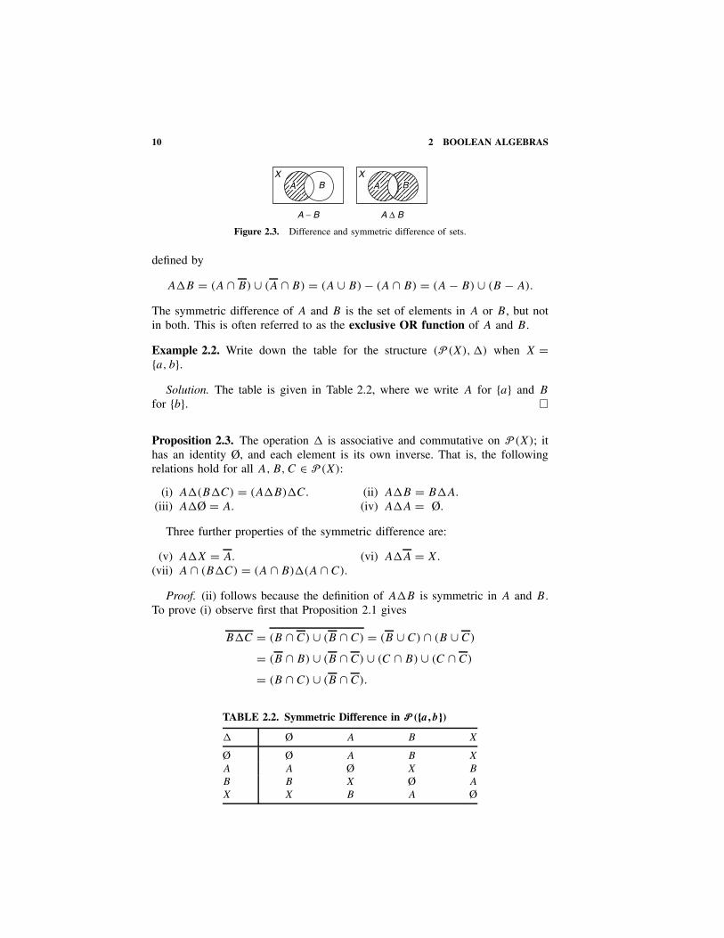
Figure 2.3. Difference and symmetric difference of sets.
defined by
A�B = (A ∩ B) ∪ (A ∩ B) = (A ∪ B) − (A ∩ B) = (A − B) ∪ (B − A).
The symmetric difference of A and B is the set of elements in A or B, but notin both. This is often referred to as the exclusive OR function of A and B.
Example 2.2. Write down the table for the structure (P (X), �) when X ={a, b}.
Solution. The table is given in Table 2.2, where we write A for {a} and B
for {b}. �
Proposition 2.3. The operation � is associative and commutative on P (X); ithas an identity Ø, and each element is its own inverse. That is, the followingrelations hold for all A,B,C ∈ P (X):
(i) A�(B�C) = (A�B)�C. (ii) A�B = B�A.(iii) A�Ø = A. (iv) A�A = Ø.
Three further properties of the symmetric difference are:
(v) A�X = A. (vi) A�A = X.(vii) A ∩ (B�C) = (A ∩ B)�(A ∩ C).
Proof. (ii) follows because the definition of A�B is symmetric in A and B.To prove (i) observe first that Proposition 2.1 gives
B�C = (B ∩ C) ∪ (B ∩ C) = (B ∪ C) ∩ (B ∪ C)
= (B ∩ B) ∪ (B ∩ C) ∪ (C ∩ B) ∪ (C ∩ C)
= (B ∩ C) ∪ (B ∩ C).
TABLE 2.2. Symmetric Difference in P ({a , b})� Ø A B X
Ø Ø A B X
A A Ø X B
B B X Ø A
X X B A Ø

NUMBER OF ELEMENTS IN A SET 11
A ∆ (B ∆ C) = (A ∆ B) ∆ C A ∩ (B ∆ C) = (A ∩ B) ∆ (A ∩ C)
A B
C
A B
C
Figure 2.4. Venn diagrams.
A ∪ (B ∆ C)
A B
C
(A ∪ B) ∆ (A ∪ C)
A B
C
Figure 2.5. Venn diagrams of unequal expressions.
Hence
A�(B�C) = {A ∩ (B�C)} ∪ {A ∩ (B�C)}= {A ∩ [(B ∩ C) ∪ (B ∩ C)]} ∪ {A ∩ [(B ∩ C) ∪ (B ∩ C)]}= (A ∩ B ∩ C) ∪ (A ∩ B ∩ C) ∪ (A ∩ B ∩ C) ∪ (A ∩ B ∩ C)).
This expression is symmetric in A, B, and C, so (ii) gives
A�(B�C) = C�(A�B) = (A�B)�C.
We leave the proof of the other parts to the reader. Parts (i) and (vii) areillustrated in Figure 2.4. �
Relation (vii) of Proposition 2.3 is a distributive law and states that ∩ isdistributive over �. It is natural to ask whether ∪ is distributive over �.
Example 2.4. Is it true that A ∪ (B�C) = (A ∪ B)�(A ∪ C) for all A,B,C ∈P (X)?
Solution. The Venn diagrams for each side of the equation are given inFigure 2.5. If the shaded areas are not the same, we will be able to find acounter example. We see from the diagrams that the result will be false ifA is nonempty. If A = X and B = C = Ø, then A ∪ (B�C) = A, whereas(A ∪ B)�(A ∪ C) = Ø; thus union is not distributive over symmetric difference.
�
NUMBER OF ELEMENTS IN A SET
If a set X contains two or three elements, we have seen that P (X) contains 22
or 23 elements, respectively. This suggests the following general result on thenumber of subsets of a finite set.

12 2 BOOLEAN ALGEBRAS
Theorem 2.5. If X is a finite set with n elements, then P (X) contains 2n
elements.
Proof. Each of the n elements of X is either in a given subset A or not in A.Hence, in choosing a subset of X, we have two choices for each element, andthese choices are independent. Therefore, the number of choices is 2n, and thisis the number of subsets of X.
If n = 0, then X = Ø and P (X) = {Ø}, which contains one element. �
Denote the number of elements of a set X by |X|. If A and B are finitedisjoint sets (that is, A ∩ B = Ø), then
|A ∪ B| = |A| + |B|.
Proposition 2.6. For any two finite sets A and B,
|A ∪ B| = |A| + |B| − |A ∩ B|.
Proof. We can express A ∪ B as the disjoint union of A and B − A; also,B can be expressed as the disjoint union of B − A and A ∩ B as shown inFigure 2.6. Hence |A ∪ B| = |A| + |B − A| and |B| = |B − A| + |A ∩ B|. It fol-lows that |A ∪ B| = |A| + |B| − |A ∩ B|. �
Proposition 2.7. For any three finite sets A, B, and C,
|A ∪ B ∪ C| = |A| + |B| + |C| − |A ∩ B| − |A ∩ C|− |B ∩ C| + |A ∩ B ∩ C|.
Proof. Write A ∪ B ∪ C as (A ∪ B) ∪ C. Then, by Proposition 2.6,
|A ∪ B ∪ C| = |A ∪ B| + |C| − |(A ∪ B) ∩ C|= |A| + |B| − |A ∩ B| + |C| − |(A ∩ C) ∪ (B ∩ C)|= |A| + |B| + |C| − |A ∩ B| − |A ∩ C| − |B ∩ C|
+ |(A ∩ C) ∩ (B ∩ C)|.
The result follows because (A ∩ C) ∩ (B ∩ C) = A ∩ B ∩ C. �
A B − A B − AA ∩ B
Figure 2.6

BOOLEAN ALGEBRAS 13
W
BC520 60
120
1020
110
200
Figure 2.7. Different classes of commuters.
Example 2.8. A survey of 1000 commuters reported that 850 sometimes used acar, 200 a bicycle, and 350 walked, whereas 130 used a car and a bicycle, 220used a car and walked, 30 used a bicycle and walked, and 20 used all three. Arethese figures consistent?
Solution. Let C, B, and W be the sets of commuters who sometimes used acar, a bicycle, and walked, respectively. Then
|C ∪ B ∪ W | = |C| + |B| + |W | − |C ∩ B| − |C ∩ W |− |B ∩ W | + |C ∩ B ∩ W |
= 850 + 200 + 350 − 130 − 220 − 30 + 20
= 1040.
Since this number is greater than 1000, the figures must be inconsistent. Thebreakdown of the reported figures into their various classes is illustrated inFigure 2.7. The sum of all these numbers is 1040. �
Example 2.9. If 47% of the people in a community voted in a local election and75% voted in a federal election, what is the least percentage that voted in both?
Solution. Let L and F be the sets of people who voted in the local and federalelections, respectively. If n is the total number of voters in the community, then|L| + |F | − |L ∩ F | = |L ∪ F | � n. It follows that
|L ∩ F | � |L| + |F | − n =(
47
100+ 75
100− 1
)n = 22
100n.
Hence at least 22% voted in both elections. �
BOOLEAN ALGEBRAS
We now give the definition of an abstract boolean algebra in terms of a setwith two binary operations and one unary operation on it. We show that variousalgebraic structures, such as the algebra of sets, the logic of propositions, and
14 2 BOOLEAN ALGEBRAS
the algebra of switching circuits are all boolean algebras. It then follows thatany general result derived from the axioms will hold in all our examples ofboolean algebras.
It should be noted that this axiom system is only one of many equivalent waysof defining a boolean algebra. Another common way is to define a boolean algebraas a lattice satisfying certain properties (see the section “Posets and Lattices”).
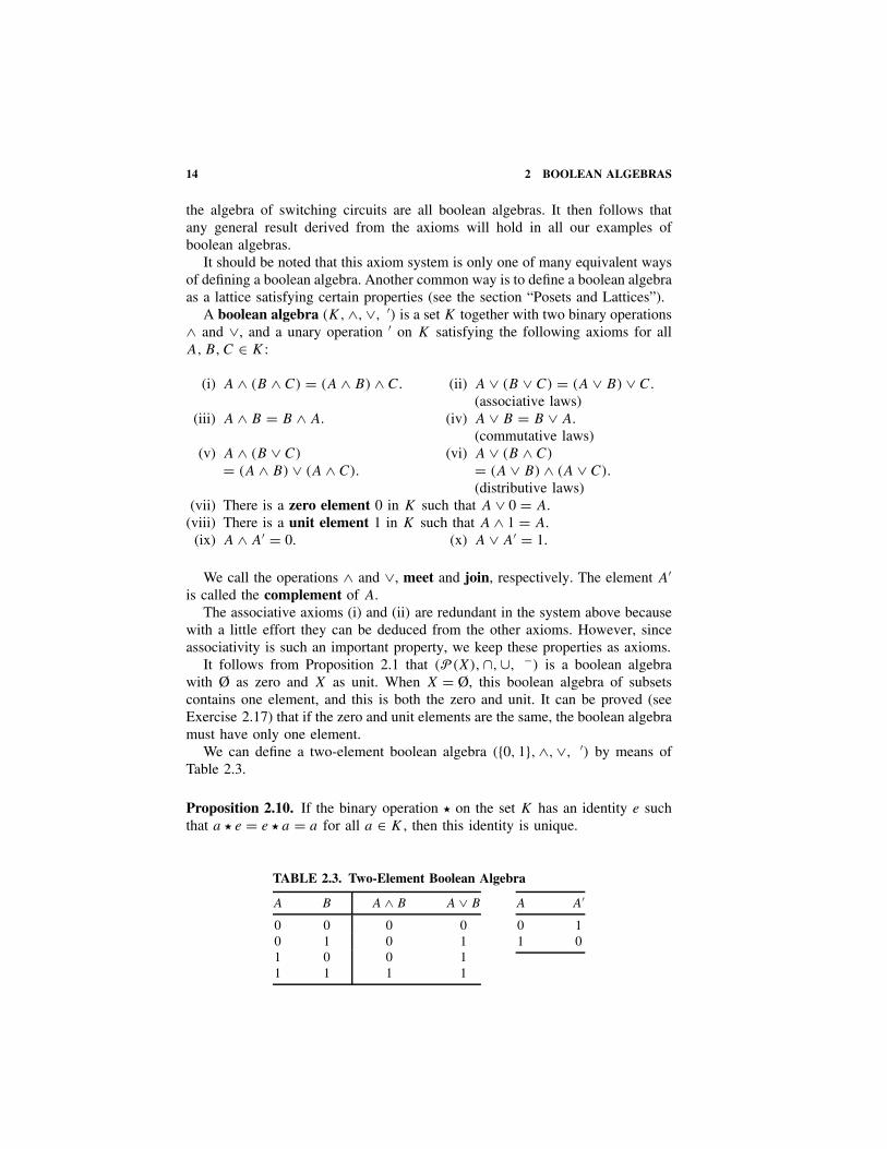
A boolean algebra (K, ∧, ∨, ′) is a set K together with two binary operations∧ and ∨, and a unary operation ′ on K satisfying the following axioms for allA, B,C ∈ K :
(i) A ∧ (B ∧ C) = (A ∧ B) ∧ C. (ii) A ∨ (B ∨ C) = (A ∨ B) ∨ C.(associative laws)
(iii) A ∧ B = B ∧ A. (iv) A ∨ B = B ∨ A.(commutative laws)
(v) A ∧ (B ∨ C)
= (A ∧ B) ∨ (A ∧ C).(vi) A ∨ (B ∧ C)
= (A ∨ B) ∧ (A ∨ C).(distributive laws)
(vii) There is a zero element 0 in K such that A ∨ 0 = A.(viii) There is a unit element 1 in K such that A ∧ 1 = A.
(ix) A ∧ A′ = 0. (x) A ∨ A′ = 1.
We call the operations ∧ and ∨, meet and join, respectively. The element A′is called the complement of A.
The associative axioms (i) and (ii) are redundant in the system above becausewith a little effort they can be deduced from the other axioms. However, sinceassociativity is such an important property, we keep these properties as axioms.
It follows from Proposition 2.1 that (P (X), ∩, ∪, −) is a boolean algebrawith Ø as zero and X as unit. When X = Ø, this boolean algebra of subsetscontains one element, and this is both the zero and unit. It can be proved (seeExercise 2.17) that if the zero and unit elements are the same, the boolean algebramust have only one element.
We can define a two-element boolean algebra ({0, 1}, ∧,∨, ′) by means ofTable 2.3.
Proposition 2.10. If the binary operation � on the set K has an identity e suchthat a � e = e � a = a for all a ∈ K , then this identity is unique.
TABLE 2.3. Two-Element Boolean Algebra
A B A ∧ B A ∨ B
0 0 0 00 1 0 11 0 0 11 1 1 1
A A′
0 11 0

BOOLEAN ALGEBRAS 15
Proof. Suppose that e and e′ are both identities. Then e = e � e′, since e′ isan identity, and e � e′ = e′ since e is an identity. Hence e = e′, so the identitymust be unique. �
Corollary 2.11. The zero and unit elements in a boolean algebra are unique.
Proof. This follows directly from the proposition above, because the zeroand unit elements are the identities for the join and meet operations, respec-tively. �
Proposition 2.12. The complement of an element in a boolean algebra is unique;that is, for each A ∈ K there is only one element A′ ∈ K satisfying axioms (ix)and (x): A ∧ A′ = 0 and A ∨ A′ = 1.
Proof. Suppose that B and C are both complements of A, so that A ∧ B =0, A ∨ B = 1, A ∧ C = 0, and A ∨ C = 1. Then
B = B ∨ 0 = B ∨ (A ∧ C) = (B ∨ A) ∧ (B ∨ C)
= (A ∨ B) ∧ (B ∨ C) = 1 ∧ (B ∨ C) = B ∨ C.
Similarly, C = C ∨ B and so B = B ∨ C = C ∨ B = C. �
If we interchange ∧ and ∨ and interchange 0 and 1 in the system of axiomsfor a boolean algebra, we obtain the same system. Therefore, if any propositionis derivable from the axioms, so is the proposition obtained by interchanging∧ and ∨ and interchanging 0 and 1. This is called the duality principle. Forexample, in the following proposition, there are four pairs of dual statements. Ifone member of each pair can be proved, the other will follow directly from theduality principle.
If (K, ∧, ∨, ′) is a boolean algebra with 0 as zero and 1 as unit, then (K, ∨, ∧, ′)is also a boolean algebra with 1 as zero and 0 as unit.
Proposition 2.13. If A, B, and C are elements of a boolean algebra (K, ∧, ∨, ′),the following relations hold:
(i) A ∧ 0 = 0. (ii) A ∨ 1 = 1.(iii) A ∧ (A ∨ B) = A. (iv) A ∨ (A ∧ B) = A.
(absorption laws)(v) A ∧ A = A. (vi) A ∨ A = A. (idempotent laws)
(vii) (A ∧ B)′ = A′ ∨ B ′. (viii) (A ∨ B)′ = A′ ∧ B ′.(De Morgan’s laws)
(ix) (A′)′ = A.
Proof. Note first that relations (ii), (iv), (vi), and (viii) are the duals of relations(i), (iii), (v), and (vii), so we prove the last four, and relation (ix). We use theaxioms for a boolean algebra several times.

16 2 BOOLEAN ALGEBRAS
(i) A ∧ 0 = A ∧ (A ∧ A′) = (A ∧ A) ∧ A′ = A ∧ A′ = 0.
(iii) A ∧ (A ∨ B) = (A ∨ 0) ∧ (A ∨ B) = A ∨ (0 ∧ B) = A ∨ 0 = A.
(v) A = A ∧ 1 = A ∧ (A ∨ A′) = (A ∧ A) ∨ (A ∧ A′)= (A ∧ A) ∨ 0 = A ∧ A.
Relations (vii) follows from Proposition 2.12 if we can show that A′ ∨ B ′ isa complement of A ∧ B [then it is the complement (A ∧ B)′]. Now using part(i) of this proposition,
(A ∧ B) ∧ (A′ ∨ B ′) = [(A ∧ B) ∧ A′] ∨ [(A ∧ B) ∧ B ′]
= [(A ∧ A′) ∧ B] ∨ [A ∧ (B ∧ B ′)]
= [0 ∧ B] ∨ [A ∧ 0]
= 0 ∨ 0
= 0.
Similarly, part (ii) gives
(A ∧ B) ∨ (A′ ∨ B ′) = [A ∨ (A′ ∨ B ′)] ∧ [B ∨ (A′ ∨ B ′)]
= [(A ∨ A′) ∨ B ′] ∧ [(B ∨ B ′) ∨ A′]
= [1 ∨ B ′] ∧ [1 ∨ A′]
= 1 ∧ 1
= 1.
To prove relation (ix), by definition we have A′ ∧ A = 0 and A′ ∨ A = 1.Therefore, A is a complement of A′, and since the complement is unique,A = (A′)′. �
PROPOSITIONAL LOGIC
We now show briefly how boolean algebra can be applied to the logic of propo-sitions. Consider two sentences “A” and “B”, which may either be true or false.For example, “A” could be “This apple is red,” and “B” could be “This pearis green.” We can combine these to form other sentences, such as “A and B,”which would be “This apple is red, and this pear is green.” We could also formthe sentence “not A,” which would be “This apple is not red.” Let us now com-pare the truth or falsity of the derived sentences with the truth or falsity of theoriginal ones. We illustrate the relationship by means of a diagram called a truthtable. Table 2.4 shows the truth tables for the expressions “A and B,” “A or B,”and “not A.” In these tables, T stands for “true” and F stands for “false.” For

PROPOSITIONAL LOGIC 17
TABLE 2.4. Truth Tables
A B A and B A or B
F F F FF T F TT F F TT T T T
A Not A
F TT F
example, if the statement “A” is true while “B” is false, the statement “A andB” will be false, and the statement “A or B” will be true.
We can have two seemingly different sentences with the same meaning; forexample, “This apple is not red or this pear is not green” has the same meaningas “It is not true that this apple is red and that this pear is green.” If twosentences, P and Q, have the same meaning, we say that P and Q are logicallyequivalent, and we write P = Q. The example above concerning apples andpears implies that
(not A) or (not B) = not (A and B).
This equation corresponds to De Morgan’s law in a boolean algebra.It appears that a set of sentences behaves like a boolean algebra. To be more
precise, let us consider a set of sentences that are closed under the operations of“and,” “or,” and “not.” Let K be the set, each element of which consists of allthe sentences that are logically equivalent to a particular sentence. Then it canbe verified that (K , and, or, not) is indeed a boolean algebra. The zero elementis called a contradiction, that is, a statement that is always false, such as “Thisapple is red and this apple is not red.” The unit element is called a tautology, thatis, a statement that is always true, such as “This apple is red or this apple is notred.” This allows us to manipulate logical propositions using formulas derivedfrom the axioms of a boolean algebra.
An important method of combining two statements, A and B, in a sentence isby a conditional, such as “If A, then B,” or equivalently, “A implies B,” whichwe shall write as “A ⇒ B.” How does the truth or falsity of such a conditionaldepend on that of A and B? Consider the following sentences:
1. If x > 4, then x2 > 16.2. If x > 4, then x2 = 2.3. If 2 = 3, then 0.2 = 0.3.4. If 2 = 3, then the moon is made of green cheese.
Clearly, if A is true, then B must also be true for the sentence “A ⇒ B”to be true. However, if A is not true, then the sentence “If A, then B” hasno standard meaning in everyday language. Let us take “A ⇒ B” to mean thatwe cannot have A true and B not true. This implies that the truth value of the

18 2 BOOLEAN ALGEBRAS
TABLE 2.5. Truth tables for Conditional andBiconditional Statements
A B A ⇒ B A ⇐ B A ⇔ B
F F T T TF T T F FT F F T FT T T T T
statement “A ⇒ B” is the same as that of “not (A and not B).” Let us write∧, ∨, and ′ for “and,” “or,” and “not,” respectively. Then “A ⇒ B” is equivalentto (A ∧ B ′)′ = A′ ∨ B. Thus “A ⇒ B” is true if A is false or if B is true.Using this definition, statements 1, 3, and 4 are all true, whereas statement 2is false.
We can combine two conditional statements to form a biconditional statementof the form “A if and only if B” or “A ⇔ B.” This has the same truth value as“(A ⇒ B) and (B ⇒ A)” or, equivalently, (A ∧ B) ∨ (A′ ∧ B ′). Another wayof expressing this biconditional is to say that “A is a necessary and sufficientcondition for B.” It is seen from Table 2.5 that the statement “A ⇔ B” is true ifeither A and B are both true or A and B are both false.
Example 2.14. Apply this propositional calculus to determine whether a certainpolitician’s arguments are consistent. In one speech he states that if taxes areraised, the rate of inflation will drop if and only if the value of the dollar doesnot fall. On television, he says that if the rate of inflation decreases or the valueof the dollar does not fall, taxes will not be raised. In a speech abroad, he statesthat either taxes must be raised or the value of the dollar will fall and the rate ofinflation will decrease. His conclusion is that taxes will be raised, but the rate ofinflation will decrease, and the value of the dollar will not fall.
Solution. We write
A to mean “Taxes will be raised,”B to mean “The rate of inflation will decrease,”C to mean “The value of the dollar will not fall.”
The politician’s three statements can be written symbolically as
(i) A ⇒ (B ⇔ C).(ii) (B ∨ C) ⇒ A′.
(iii) A ∨ (C′ ∧ B).
His conclusion is (iv) A ∧ B ∧ C.The truth values of the first two statements are equivalent to those of the
following:
SWITCHING CIRCUITS 19
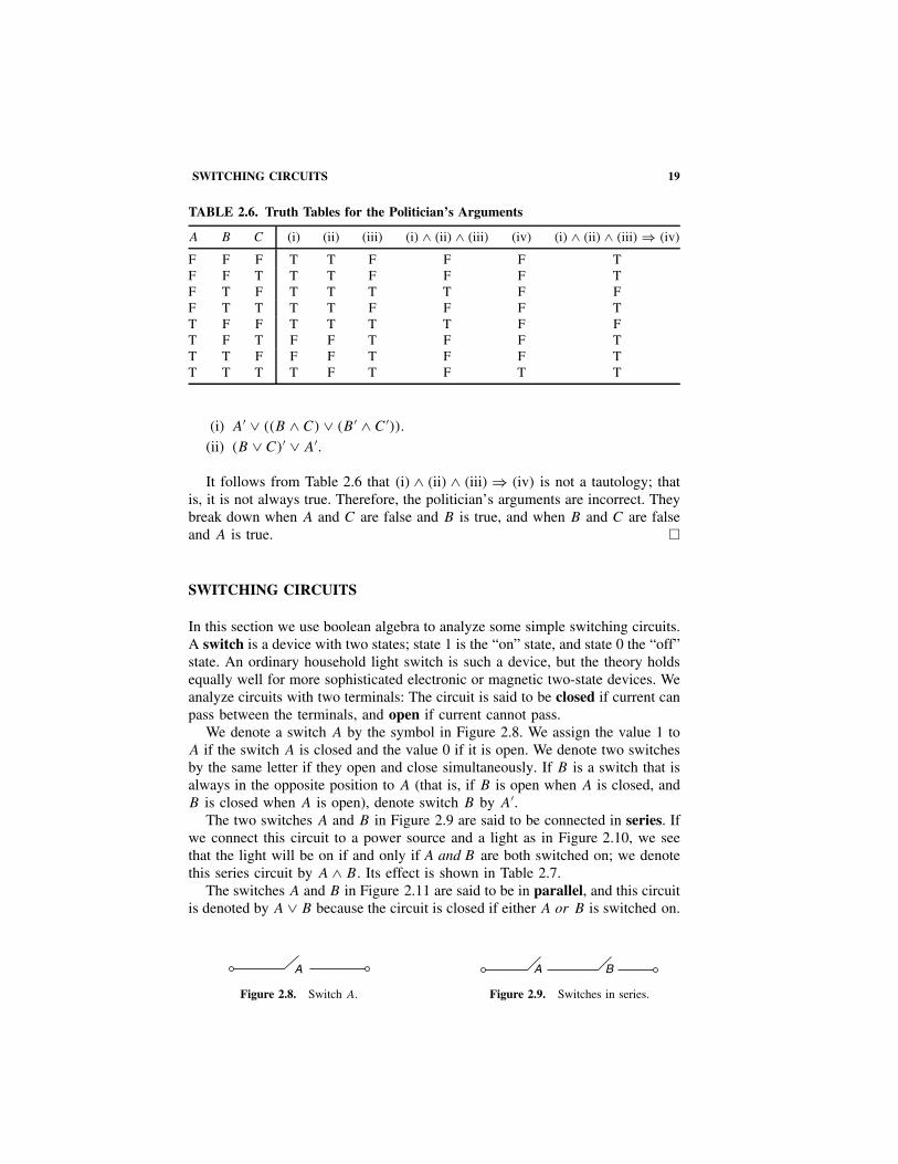
TABLE 2.6. Truth Tables for the Politician’s Arguments
A B C (i) (ii) (iii) (i) ∧ (ii) ∧ (iii) (iv) (i) ∧ (ii) ∧ (iii) ⇒ (iv)
F F F T T F F F TF F T T T F F F TF T F T T T T F FF T T T T F F F TT F F T T T T F FT F T F F T F F TT T F F F T F F TT T T T F T F T T
(i) A′ ∨ ((B ∧ C) ∨ (B ′ ∧ C′)).(ii) (B ∨ C)′ ∨ A′.
It follows from Table 2.6 that (i) ∧ (ii) ∧ (iii) ⇒ (iv) is not a tautology; thatis, it is not always true. Therefore, the politician’s arguments are incorrect. Theybreak down when A and C are false and B is true, and when B and C are falseand A is true. �
SWITCHING CIRCUITS
In this section we use boolean algebra to analyze some simple switching circuits.A switch is a device with two states; state 1 is the “on” state, and state 0 the “off”state. An ordinary household light switch is such a device, but the theory holdsequally well for more sophisticated electronic or magnetic two-state devices. Weanalyze circuits with two terminals: The circuit is said to be closed if current canpass between the terminals, and open if current cannot pass.
We denote a switch A by the symbol in Figure 2.8. We assign the value 1 toA if the switch A is closed and the value 0 if it is open. We denote two switchesby the same letter if they open and close simultaneously. If B is a switch that isalways in the opposite position to A (that is, if B is open when A is closed, andB is closed when A is open), denote switch B by A′.
The two switches A and B in Figure 2.9 are said to be connected in series. Ifwe connect this circuit to a power source and a light as in Figure 2.10, we seethat the light will be on if and only if A and B are both switched on; we denotethis series circuit by A ∧ B. Its effect is shown in Table 2.7.
The switches A and B in Figure 2.11 are said to be in parallel, and this circuitis denoted by A ∨ B because the circuit is closed if either A or B is switched on.
A
Figure 2.8. Switch A.
A B
Figure 2.9. Switches in series.

20 2 BOOLEAN ALGEBRAS
A B
Power source Light
Figure 2.10. Series circuit.
A
B
Figure 2.11. Switches in parallel.
TABLE 2.7. Effect of the Series Circuit
Switch A Switch B Circuit A ∧ B Light
0 (off) 0 (off) 0 (open) off0 (off) 1 (on) 0 (open) off1 (on) 0 (off) 0 (open) off1 (on) 1 (on) 1 (closed) on
A
A ′
B ′
B
Figure 2.12. Series-parallel circuit.
The reader should be aware that many books on switching theory use thenotation + and · instead of ∨ and ∧, respectively.
Series and parallel circuits can be combined to form circuits like the one inFigure 2.12. This circuit would be denoted by (A ∨ (B ∧ A′)) ∧ B ′. Such circuitsare called series-parallel switching circuits.
In actual practice, the wiring diagram may not look at all like Figure 2.12,because we would want switches A and A′ together and B and B ′ together.Figure 2.13 illustrates one particular form that the wiring diagram could take.
Two circuits C1 and C2 involving the switches A, B, . . . are said to be equiv-alent if the positions of the switches A, B, . . ., which allow current to pass,
Switch A
Switch B
Figure 2.13. Wiring diagram of the circuit.
DIVISORS 21
A
B
C
A B
A C
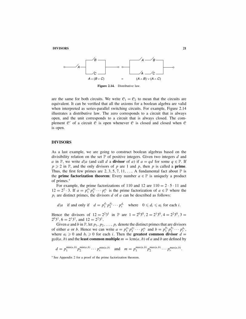
A ∧ (B ∨ C) (A ∧ B) ∨ (A ∧ C)=
Figure 2.14. Distributive law.
are the same for both circuits. We write C1 = C2 to mean that the circuits areequivalent. It can be verified that all the axioms for a boolean algebra are validwhen interpreted as series-parallel switching circuits. For example, Figure 2.14illustrates a distributive law. The zero corresponds to a circuit that is alwaysopen, and the unit corresponds to a circuit that is always closed. The com-plement C ′ of a circuit C is open whenever C is closed and closed when Cis open.
DIVISORS
As a last example, we are going to construct boolean algebras based on thedivisibility relation on the set P of positive integers. Given two integers d anda in P, we write d|a (and call d a divisor of a) if a = qd for some q ∈ P. Ifp � 2 in P, and the only divisors of p are 1 and p, then p is called a prime.Thus, the first few primes are 2, 3, 5, 7, 11, . . .. A fundamental fact about P isthe prime factorization theorem: Every number a ∈ P is uniquely a productof primes.∗
For example, the prime factorizations of 110 and 12 are 110 = 2 · 5 · 11 and12 = 22 · 3. If a = p
a11 p
a22 · · · par
r is the prime factorization of a ∈ P where thepi are distinct primes, the divisors d of a can be described as follows:
d|a if and only if d = pd11 p
d22 · · · pdr
r where 0 � di � ai for each i.
Hence the divisors of 12 = 2231 in P are 1 = 2030, 2 = 2130, 4 = 2230, 3 =2031, 6 = 2131, and 12 = 2231.
Given a and b in P, let p1, p2, . . . , pr denote the distinct primes that are divisorsof either a or b. Hence we can write a = p
a11 p
a22 · · · par
r and b = pb11 p
b22 · · · pbr
r ,where ai � 0 and bi � 0 for each i. Then the greatest common divisor d =gcd(a, b) and the least common multiple m = lcm(a, b) of a and b are defined by
d = pmin(a,b)
1 pmin(a,b)
2 · · ·pmin(a,b)r and m = p
max(a,b)
1 pmax(a,b)
2 · · · pmax(a,b)r .
∗ See Appendix 2 for a proof of the prime factorization theorem.

22 2 BOOLEAN ALGEBRAS
It follows that d is the unique integer in P that is a divisor of both a and b, andis a multiple of every such common divisor (hence the name). Similarly, m isthe unique integer in P that is a multiple of both a and b, and is a divisor ofevery such common multiple. For example, gcd(2, 3) = 1 and gcd(12, 28) = 4,while lcm(2, 3) = 6 and lcm(12, 28) = 84.
With this background, we can describe some new examples of boolean alge-bras. Given n ∈ P, let
Dn = {d ∈ P|d divides n}.
It is clear that gcd and lcm are commutative binary operations on Dn, and it iseasy to verify that the zero is 1 and the unit is n. To prove the distributive laws,let a, b, and c be elements of Dn, and write
a = pa11 p
a22 · · ·par
r , b = pb11 p
b22 · · · pbr
r , and c = pc11 p
c22 · · ·pcr
r ,
where p1, p2, . . . , pr are the distinct primes dividing at least one of a, b, and c,and where ai � 0, bi � 0, and ci � 0 for each i. Then the first distributive lawstates that
gcd(a, lcm(b, c)) = lcm(gcd(a, b), gcd(a, c)).
If we write out the prime factorization of each side in terms of the primes pi , thisholds if and only if for each i, the powers of pi are equal on both sides, that is,
min(ai, max(bi, ci)) = max(min(ai, bi), min(ai, ci)).
To verify this, observe first that we may assume that bi � ci (bi and ci can beinterchanged without changing either side), and then check the three cases ai �bi, bi � ai � ci , and ci � ai separately. Hence the first distributive law holds; theother distributive law and the associative laws are verified similarly. Thus (Dn,gcd, lcm) satisfies all the axioms for a boolean algebra except for the existenceof a complement.
But complements need not exist in general: For example, 6 has no comple-ment in D18 = {1, 2, 3, 6, 9, 18}. Indeed, if 6 has a complement 6′ in D18, thengcd(6, 6′) = 1, so we must have 6′ = 1. But then lcm(6, 6′) = 6 and this is notthe unit of D18. Hence 6 has no complement, so D18 is not a boolean alge-bra. However, all is not lost. The problem in D18 is that the prime factorization18 = 2 · 32 has a repeated prime factor. An integer n ∈ P is called square-freeif it is a product of distinct primes with none repeated (for example, every primeis square-free, as are 6 = 2 · 3, 10 = 2 · 5, 30 = 2 · 3 · 5, etc.) If n is square-free,it is routine to verify that the complement of d ∈ Dn is d ′ = n/d , and we have
Example 2.15. If n ∈ P is square-free, then (Dn, gcd, lcm, ′) is a boolean alge-bra where d ′ = n/d for each d ∈ Dn.
The interpretations of the various boolean algebra terms are given in Table 2.8.

POSETS AND LATTICES 23
TABLE 2.8. Dictionary of Boolean Algebra Terms
BooleanAlgebra P(X)
SwitchingCircuits
PropositionalLogic Dn
∧ ∩ Series And gcd∨ ∪ Parallel Or lcm′ − Opposite Not a′ = n/a
0 Ø Open Contradiction 11 X Closed Tautology n
= = Equivalent circuit Logically equivalent =
POSETS AND LATTICES
Boolean algebras were derived from the algebra of sets, and there is one importantrelation between sets that we have neglected to generalize to boolean algebras,namely, the inclusion relation. This relation can be defined in terms of the unionoperation by
A ⊆ B if and only if A ∩ B = A.
We can define a corresponding relation � on any boolean algebra (K,∧, ∨, ′)using the meet operation:
A � B if and only if A ∧ B = A.
If the boolean algebra is the algebra of subsets of X, this relation is the usualinclusion relation.
Proposition 2.16. A ∧ B = A if and only if A ∨ B = B. Hence either of thethese conditions will define the relation �.
Proof. If A ∧ B = A, then it follows from the absorption law that A ∨ B =(A ∧ B) ∨ B = B. Similarly, if A ∨ B = B, it follows that A ∧ B = A. �
Proposition 2.17. If A, B, and C are elements of a boolean algebra, K , thefollowing properties of the relation � hold.
(i) A � A. (reflexivity)(ii) If A � B and B � A, then A = B. (antisymmetry)
(iii) If A � B and B � C, then A � C. (transitivity)
Proof
(i) A ∧ A = A is an idempotent law.(ii) If A ∧ B = A and B ∧ A = B, then A = A ∧ B = B ∧ A = B.
(iii) If A ∧ B = A and B ∧ C = B, then A ∧ C = (A ∧ B) ∧ C
= A ∧ (B ∧ C) = A ∧ B = A. �

24 2 BOOLEAN ALGEBRAS
TABLE 2.9. Partial Order Relation in Various Boolean Algebras
BooleanAlgebra
Algebra ofSubsets
Series-ParallelSwitchingCircuits
PropositionalLogic
Divisors of aSquare-Free
Integer
A ∧ B = A A ∩ B = A A ∧ B = A (A and B) = A gcd(a, b) = a
A � B A ⊆ B A ⇒ B A ⇒ B a|bA is less than
or equal to B
A is a subsetof B
If A is closed,then B isclosed
A implies B a divides b
A relation satisfying the three properties in Proposition 2.17 is called a partialorder relation, and a set with a partial order on it is called a partially orderedset or poset for short. The interpretation of the partial order in various booleanalgebras is given in Table 2.9.
A partial order on a finite set K can be displayed conveniently in a posetdiagram in which the elements of K are represented by small circles. Lines aredrawn connecting these elements so that there is a path from A to B that is alwaysdirected upward if and only if A � B. Figure 2.15 illustrates the poset diagramof the boolean algebra of subsets (P ({a, b}, )∩, ∪, −). Figure 2.16 illustratesthe boolean algebra D110 = {1, 2, 5, 11, 10, 22, 55, 110} of positive divisors of110 = 2 · 5 · 11. The partial order relation is divisibility, so that there is an upwardpath from a to b if and only if a divides b.
The following proposition shows that � has properties similar to those of theinclusion relation in sets.
Proposition 2.18. If A, B, C are elements of a boolean algebra (K, ∧,∨, ′),then the following relations hold:
(i) A ∧ B � A.(ii) A � A ∨ B.
(iii) A � C and B � C implies that A ∨ B � C.
{a, b}
{a} {b}
f
Figure 2.15. Poset diagram of P ({a, b}).
110
22 55
115
1
2
10
Figure 2.16. Poset diagram of D110.

POSETS AND LATTICES 25
(iv) A � B if and only if A ∧ B ′ = 0.
(v) 0 � A and A � 1 for all A.
Proof
(i) (A ∧ B) ∧ A = (A ∧ A) ∧ B = A ∧ B so A ∧ B � A.
(ii) A ∧ (A ∨ B) = A, so A � A ∨ B.
(iii) (A ∨ B) ∧ C = (A ∧ C) ∨ (B ∧ C) = A ∨ B.
(iv) If A � B, then A ∧ B = A and A ∧ B ′ = A ∧ B ∧ B ′ = A ∧ 0 = 0. Onthe other hand, if A ∧ B ′ = 0, then A � B because
A = A ∧ 1 = A ∧ (B ∨ B ′) = (A ∧ B) ∨ (A ∧ B ′)
= (A ∧ B) ∨ 0 = A ∧ B.
(v) 0 ∧ A = 0 and A ∧ 1 = A. �
Not all posets are derived from boolean algebras. A boolean algebra is anextremely special kind of poset. We now determine conditions which ensure thata poset is indeed a boolean algebra. Given a partial order � on a set K , we haveto find two binary operations that correspond to the meet and join.
An element d is said to be the greatest lower bound of the elements a andb in a partially ordered set if d � a, d � b, and x is another element, for whichx � a, x � b, then x � d . We denote the greatest lower bound of a and b bya ∧ b. Similarly, we can define the least upper bound and denote it by ∨. Itfollows from the antisymmetry of the partial order relation that each pair ofelements a and b can have at most one greatest lower bound and at most oneleast upper bound.
A lattice is a partially ordered set in which every two elements have a greatestlower bound and a least upper bound. Thus Dn is a lattice for every integer n ∈ P,so by the discussion preceding Example 2.15, D18 is a lattice that is not a booleanalgebra (see Figure 2.17).
We can now give an alternative definition of a boolean algebra in terms of alattice: A boolean algebra is a lattice that has universal bounds (that is, elements0 and 1 such that 0 � a and a � 1 for all elements a) and is distributive andcomplemented (that is, the distributive laws for ∧ and ∨ hold, and complementsexist). It can be verified that this definition is equivalent to our original one.
In Figure 2.18, the elements c and d have a least upper bound b but no greatestlower bound.
We note in passing that the discussion preceding Example 2.15 shows that foreach n ∈ P, the poset Dn is a lattice in which the distributive laws hold, but it isnot a boolean algebra unless n is square-free. For further reading on lattices inapplied algebra, consult, Davey and Priestley [16] or Lidl and Pilz [10].

26 2 BOOLEAN ALGEBRAS
1
2
6
3
9
18
Figure 2.17. Lattice that is not a boolean algebra.
c
a b
d
e
Figure 2.18. Poset that is not a lattice.
NORMAL FORMS AND SIMPLIFICATION OF CIRCUITS
If we have a complicated switching circuit represented by a boolean expression,such as
(A ∧ (B ∨ C′)′) ∨ ((B ∧ C′) ∨ A′),
we would like to know if we can build a simpler circuit that would perform thesame function. In other words, we would like to reduce this boolean expressionto a simpler form. In actual practice, it is usually desirable to reduce the circuit tothe one that is cheapest to build, and the form this takes will depend on the stateof the technology at the time; however, for our purposes we take the simplestform to mean the one with the fewest switches. It is difficult to find the simplestform for circuits with many switches, and there is no one method that will lead tothat form. However, we do have methods for determining whether two booleanexpressions are equivalent. We can reduce the expressions to a certain normalform, and the expressions will be the same if and only if their normal forms arethe same. We shall look at one such form, called the disjunctive normal form.
In the boolean algebra of subsets of a set, every subset can be expressed asa union of singleton sets, and this union is unique to within the ordering of theterms. We shall obtain a corresponding result for arbitrary finite boolean algebras.The elements that play the role of singleton sets are called atoms. Here an atomin a boolean algebra (K, ∧,∨, ′) is a nonzero element B for which
B ∧ Y = B or B ∧ Y = 0 for each Y ∈ K.
NORMAL FORMS AND SIMPLIFICATION OF CIRCUITS 27
Thus B is an atom if Y � B implies that Y = 0 or Y = B. This implies that theatoms are the elements immediately above the zero element in the poset diagram.In the case of the algebra of divisors of a square-free integer, the atoms are theprimes, because the definition of b being prime is that y|b implies that y = 1 ory = b.
We now give a more precise description of the algebra of switching circuits.The atoms of the algebra and the disjunctive normal form of an expression willbecome clear from this description.
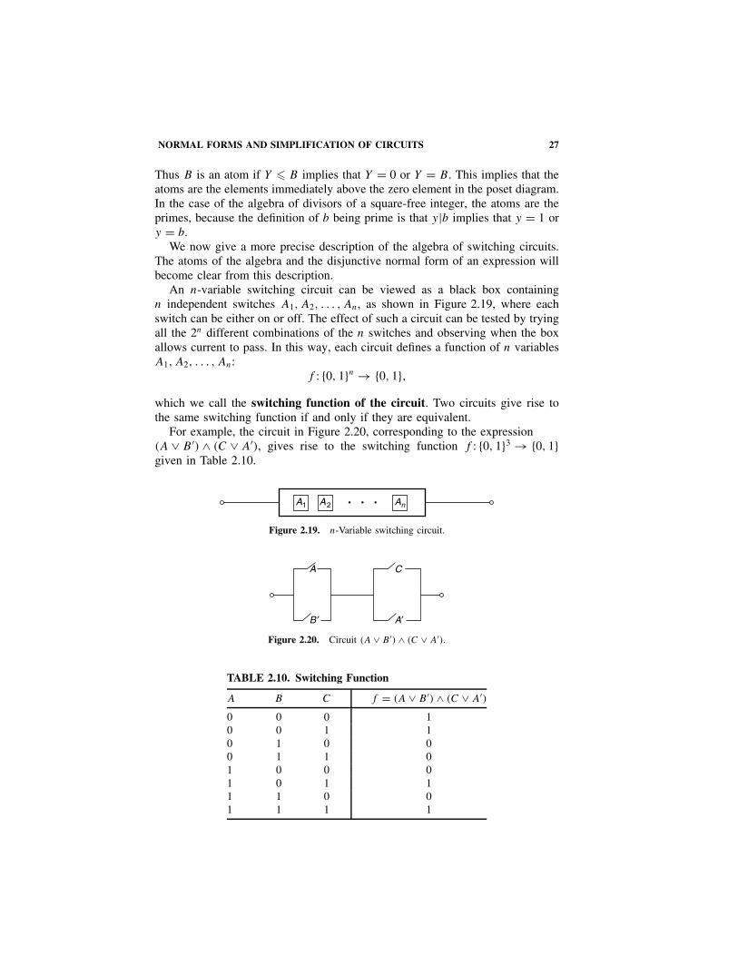
An n-variable switching circuit can be viewed as a black box containingn independent switches A1, A2, . . . , An, as shown in Figure 2.19, where eachswitch can be either on or off. The effect of such a circuit can be tested by tryingall the 2n different combinations of the n switches and observing when the boxallows current to pass. In this way, each circuit defines a function of n variablesA1, A2, . . . , An:
f : {0, 1}n → {0, 1},which we call the switching function of the circuit. Two circuits give rise tothe same switching function if and only if they are equivalent.
For example, the circuit in Figure 2.20, corresponding to the expression(A ∨ B ′) ∧ (C ∨ A′), gives rise to the switching function f : {0, 1}3 → {0, 1}given in Table 2.10.
A1 A2 An• • •
Figure 2.19. n-Variable switching circuit.
A C
A′B ′
Figure 2.20. Circuit (A ∨ B ′) ∧ (C ∨ A′).
TABLE 2.10. Switching Function
A B C f = (A ∨ B ′) ∧ (C ∨ A′)
0 0 0 10 0 1 10 1 0 00 1 1 01 0 0 01 0 1 11 1 0 01 1 1 1

28 2 BOOLEAN ALGEBRAS
Denote the set of all n-variable switching functions from {0, 1}n to {0, 1} byFn. Each of the 2n elements in the domain of such a function can be mapped toeither of the two elements in the codomain. Therefore, the number of differentn-variable switching functions, and hence the number of different circuits withn switches, is 22n
.Let f and g be the switching functions of two circuits of the n-variables
A1, A2, . . . , An. When these circuits are connected in series or in parallel, theygive rise to the switching functions f ∧ g or f ∨ g, respectively, where
(f ∧ g)(A1, . . . , An) = f (A1, . . . , An) ∧ g(A1, . . . , An)
and(f ∨ g)(A1, . . . , An) = f (A1, . . . , An) ∨ g(A1, . . . , An).
The switching function of the opposite circuit to that defining f is f ′, where
f ′(A1, . . . , An) = (f (A1, . . . , An))′.
Theorem 2.19. The set of n-variable switching functions forms a boolean alge-bra (Fn, ∧, ∨, ′) that contains 22n
elements.
Proof. It can be verified that (Fn, ∧,∨,′ ) satisfies all the axioms of a booleanalgebra. The zero element is the function whose image is always 0, and the unitelement is the function whose image is always 1. �
The boolean algebra of switching functions of two variables contains 16 ele-ments, which are displayed in Table 2.11. For example, f6(A, B) = 0 if A = B,and 1 if A �= B. This function is the exclusive OR function or a modulo 2 adder.It is also the symmetric difference function, where the symmetric difference ofA and B in a boolean algebra is defined by
A�B = (A ∧ B ′) ∨ (A′ ∧ B).
The operations NAND and NOR stand for “not and” and “not or,” respectively;these are discussed further in the section “Transistor Gates.”
As an example of the operations in the boolean algebra F2, we calculate themeet and join of f10 and f7, and the complement of f10 in Table 2.12. Wesee that f10 ∧ f7 = f2, f10 ∨ f7 = f15 and f ′
10 = f5. These correspond to therelations B ′ ∧ (A ∨ B) = A ∧ B ′, B ′ ∨ (A ∨ B) = 1, and (B ′)′ = B.
In the boolean algebra Fn, f � g if and only if f ∧ g = f , which happens ifg(A1, . . . , An) = 1 whenever f (A1, . . . , An) = 1. The atoms of Fn are thereforethe functions whose image contains precisely one nonzero element. Fn contains2n atoms, and the expressions that realize these atoms are of the formA
α11 ∧ A
α22 ∧ · · · ∧ Aαn
n , where each Aαi
i = Ai or A′i .

NORMAL FORMS AND SIMPLIFICATION OF CIRCUITS 29
TABLE 2.11. Two-Variable Switching Functions
A 0 0 1 1 Expressions in A and B
B 0 1 0 1 Representing the Function
f0 0 0 0 0 0f1 0 0 0 1 A ∧ B
f2 0 0 1 0 A ∧ B ′ or A �⇒ B
f3 0 0 1 1 A
f4 0 1 0 0 A′ ∧ B or A �⇐ B
f5 0 1 0 1 B
f6 0 1 1 0 A�B or Exclusive OR(A, B)f7 0 1 1 1 A ∨ B
f8 1 0 0 0 A′ ∧ B ′ or NOR(A, B)f9 1 0 0 1 A�B ′ or A ⇔ B
f10 1 0 1 0 B ′f11 1 0 1 1 A ∨ B ′ or A ⇐ B
f12 1 1 0 0 A′f13 1 1 0 1 A′ ∨ B or A ⇒ B
f14 1 1 1 0 A′ ∨ B ′ or NAND(A,B)f15 1 1 1 1 1
TABLE 2.12. Some Operations in F 2
A B f10 f7 f10 ∧ f7 f10 ∨ f7 f ′10
0 0 1 0 0 1 00 1 0 1 0 1 11 0 1 1 1 1 01 1 0 1 0 1 1
The 16 elements of F2 are illustrated in Figure 2.21, and the four atoms aref1, f2, f4, and f8, which are defined in Table 2.11.
To show that every element of a finite boolean algebra can be written as ajoin of atoms, we need three preliminary lemmas.
Lemma 2.20. If A, B1, . . . , Br are atoms in a boolean algebra, thenA � (B1 ∨ · · · ∨ Br) if and only if A = Bi , for some i with 1 � i � r .
Proof. If A � (B1 ∨ · · · ∨ Br), then A ∧ (B1 ∨ · · · ∨ Br) = A; thus (A ∧ B1) ∨· · · ∨ (A ∧ Br) = A. Since each Bi is an atom, A ∧ Bi = Bi or 0. Not all theelements A ∧ Bi can be 0, for this would imply that A = 0. Hence there is some i,with 1 � i � r , for which A ∧ Bi = Bi . But A is also an atom, so A = A ∧ Bi =Bi .
The implication the other way is straightforward �
Lemma 2.21. If Z is a nonzero element of a finite boolean algebra, there existsan atom B with B � Z.

30 2 BOOLEAN ALGEBRAS
f15
f11 f13f7
f3
f1
f5 f9 f6
f2
f0
f4
f10
f14
f12
f8
Figure 2.21. Poset diagram of the boolean algebra of two-variable switching functions.
Proof. If Z is an atom, take B = Z. If not, then it follows from the definitionof atoms that there exists a nonzero element Z1, different from Z, with Z1 � Z.If Z1 is not an atom, we continue in this way to obtain a sequence of distinctnonzero elements · · · � Z3 � Z2 � Z1 � Z, which, because the algebra is finite,must terminate in an atom B. �
Lemma 2.22. If B1, . . . , Bn are all the atoms of a finite boolean algebra, thenY = 0 if and only if Y ∧ Bi = 0 for all i such that 1 � i � n.
Proof. Suppose that Y ∧ Bi = 0 for each i. If Y is nonzero, it follows from theprevious lemma that there is an atom Bj with Bj � Y . Hence Bj = Y ∧ Bj = 0,which is a contradiction, so Y = 0. The converse implication is trivial. �
Theorem 2.23. Disjunctive Normal Form. Each element X of a finite booleanalgebra can be written as a join of atoms
X = Bα ∨ Bβ ∨ · · · ∨ Bω.
Moreover, this expression is unique up to the order of the atoms.
Proof. Let Bα,Bβ, . . . , Bω be all the atoms less than or equal to X in thepartial order. It follows from Proposition 2.18(iii) that the join Y = Bα ∨ Bβ ∨· · · ∨ Bω � X.
We will show that X ∧ Y ′ = 0, which, by Proposition 2.18(iv), is equivalentto X � Y . We have
X ∧ Y ′ = X ∧ B ′α ∧ · · · ∧ B ′
ω.
If B is an atom in the join Y , say B = Bα, it follows that X ∧ Y ′ ∧ B = 0,since B ′
α ∧ Bα = 0. If B is an atom that is not in Y , then X ∧ Y ′ ∧ B = 0 also,
NORMAL FORMS AND SIMPLIFICATION OF CIRCUITS 31
because X ∧ B = 0. Therefore, by Lemma 2.22, X ∧ Y ′ = 0, which is equivalentto X � Y . The antisymmetry of the partial order relation implies that X = Y .
To show uniqueness, suppose that X can be written as the join of two setsof atoms
X = Bα ∨ · · · ∨ Bω = Ba ∨ · · · ∨ Bz.
Now Bα � X; thus, by Lemma 2.20, Bα is equal to one of the atoms on theright-hand side, Ba, . . . , Bz. Repeating this argument, we see that the two sets ofatoms are the same, except possibly for their order. �
In the boolean algebra of n-variable switching functions, the atoms are realizedby expressions of the form A
α11 ∧ A
α22 ∧ · · · ∧ An
αn , where the αi’s are 0 or 1 andAi
αi = Ai , if αi = 1, whereas Aiαi = A′
i , if αi = 0. The expression Aα11 ∧ A
α22 ∧
· · · ∧ Anαn is included in the disjunctive normal form of the function f if and
only if f (α1, α2, . . . , αn) = 1. Hence there is one atom in the disjunctive normalform for each time the element 1 occurs in the image of the switching function.
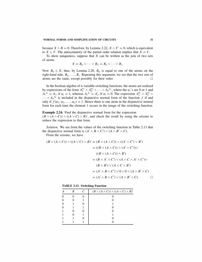
Example 2.24. Find the disjunctive normal form for the expression(B ∨ (A ∧ C)) ∧ ((A ∨ C) ∧ B)′, and check the result by using the axioms toreduce the expression to that form.
Solution. We see from the values of the switching function in Table 2.13 thatthe disjunctive normal form is (A′ ∧ B ∧ C′) ∨ (A ∧ B ′ ∧ C).
From the axioms, we have
(B ∨ (A ∧ C)) ∧ ((A ∨ C) ∧ B)′ = (B ∨ (A ∧ C)) ∧ ((A′ ∧ C′) ∨ B ′)
= ((B ∨ (A ∧ C)) ∧ (A′ ∧ C′))∨((B ∨ (A ∧ C)) ∧ B ′)
= (B ∧ A′ ∧ C′) ∨ (A ∧ C ∧ A′ ∧ C′)∨(B ∧ B ′) ∨ (A ∧ C ∧ B ′)
= (A′ ∧ B ∧ C′) ∨ 0 ∨ 0 ∨ (A ∧ B ′ ∧ C)
= (A′ ∧ B ∧ C′) ∨ (A ∧ B ′ ∧ C). �
TABLE 2.13. Switching Function
A B C (B ∨ (A ∧ C)) ∧ ((A ∨ C) ∧ B)′
0 0 0 00 0 1 00 1 0 10 1 1 01 0 0 01 0 1 11 1 0 01 1 1 0

32 2 BOOLEAN ALGEBRAS
TABLE 2.14. Switching Function
A B (A ∨ B) ∧ B ′ (A ∨ B) ∧ (A ∧ B)′ (A ∧ B)′ ∧ (A ∧ B ′)
0 0 0 0 00 1 0 1 01 0 1 1 11 1 0 0 0
Example 2.25. Determine whether any of the three expressions(A ∨ B) ∧ B ′, (A ∨ B) ∧ (A ∧ B)′, and (A ∧ B)′ ∧ (A ∧ B ′) equivalent.
Solution. We see from Table 2.14 that (A ∨ B) ∧ B ′ = (A ∧ B)′ ∧ (A ∧ B ′)and that these are both equal to A ∧ B ′. �
The atoms in the boolean algebra F2 are realized by the expressionsA′ ∧ B ′, A′ ∧ B,A ∧ B ′, and A ∧ B. These atoms partition the Venn diagramin Figure 2.22 into four disjoint regions. The disjunctive normal form for anyboolean expression involving the variables A and B can be calculated by shadingthe region of the Venn diagram corresponding to the expression and then takingthe join of the atoms in the shaded region. Figure 2.23 illustrates the eight regionsof the corresponding Venn diagram for three variables.
A
A ∧ B ′ A ∧ B A′ ∧ B
A′ ∧ B ′
B
Figure 2.22. Venn diagram for F2.
A ∧ B ′ ∧ C ′ A′ ∧ B ∧ C ′A ∧ B ∧ C ′
A ∧ B ∧ C
A′ ∧ B ′ ∧ C
A′ ∧ B ′ ∧ C ′
A ∧ B ′ ∧ C A′ ∧ B ∧ C
A B
C
Figure 2.23. Venn diagram for F3.

NORMAL FORMS AND SIMPLIFICATION OF CIRCUITS 33
By looking at the shaded region of a Venn diagram corresponding to a booleanexpression, it is often possible to see how to simplify the expression. Furthermore,the disjunctive normal form provides a method of proving hypotheses derivedfrom these Venn diagrams.
However, Venn diagrams become too complicated and impractical for func-tions of more than four variables. For other general methods of simplifyingcircuits, consult a book on boolean algebras such as Mendelson [21].
Example 2.26. Find the disjunctive normal form and simplify the circuit inFigure 2.24.
Solution. This circuit is represented by the boolean expression
f = A ∨ ((B ′ ∨ C) ∧ (A ∨ B ∨ C)).
The boolean function f : {0, 1}3 → {0, 1} that this expression defines is given inTable 2.15. It follows that the disjunctive normal form is
(A′ ∧ B ′ ∧ C) ∨ (A′ ∧ B ∧ C) ∨ (A ∧ B ′ ∧ C′) ∨ (A ∧ B ′ ∧ C)
∨ (A ∧ B ∧ C′) ∨ (A ∧ B ∧ C),
which is certainly not simpler than the original. However, by looking at the Venndiagram in Figure 2.25, we see that this expression is equivalent to just A ∨ C;thus a simpler equivalent circuit is given in Figure 2.25. �
A
A
B
C
B ′
C
Figure 2.24. Series-parallel circuit.
TABLE 2.15. SwitchingFunction
A B C f
0 0 0 00 0 1 10 1 0 00 1 1 11 0 0 11 0 1 11 1 0 11 1 1 1

34 2 BOOLEAN ALGEBRAS
AA
C
B
C
Figure 2.25. Venn diagram and simplified circuit.
In building a computer, one of the most important pieces of equipment neededis a circuit that will add two numbers in binary form. Consider the problem ofadding the numbers 15 and 5. Their binary forms are 1111 and 101, respectively.The binary and decimal additions are shown below. In general, if we add thenumber . . . a2a1a0 to . . . b2b1b0, we have to carry the digits . . . c2c1 to obtain thesum . . . s2s1s0.
1111 15 . . . a2a1a0
101 5 . . . b2b1b0
1111 ← carry digits → 1 . . . c2c1
10100 20 . . . s2s1s0
binary addition decimal addition
Let us first design a circuit to add a0 and b0 to obtain s0 and the carry digitc1. This is called a half adder. The digits s0 and c1 are functions of a0 and b0
which are given by Table 2.16. For example, in binary arithmetic, 1 + 1 = 10,which means that if a0 = 1 and b0 = 1, s0 = 0, and we have to carry c1 = 1.
We see from Table 2.16 that c1 = a0 ∧ b0 and s0 = (a′0 ∧ b0) ∨ (a0 ∧ b′
0).These circuits are shown in Figure 2.26.
TABLE 2.16. SwitchingFunctions for the HalfAdder
a0 b0 c1 s0
0 0 0 00 1 0 11 0 0 11 1 1 0
a ′0 b0
b0 c1
s0
a0
a0
b ′0
Figure 2.26. Circuits for the half adder.

NORMAL FORMS AND SIMPLIFICATION OF CIRCUITS 35
TABLE 2.17. Switching Functionsfor a Full Adder
ai bi ci ci+1 si
0 0 0 0 00 0 1 0 10 1 0 0 10 1 1 1 01 0 0 0 11 0 1 1 01 1 0 1 0
1 1 1 1 1
ai bi
ci +1 shaded
si shaded
ci
ai bi
ci
Figure 2.27. Venn diagrams for a full adder.
a ′ib ′i
c ′i
c ′i
ci
ci
si
ci +1ci
ci
ai
ai
bi
b ′i
bi
bi
bi
Figure 2.28. Circuits for a full adder.
A circuit that adds ai, bi , and the carry digit, ci , to obtain si , with ci+1 tocarry, is called a full adder. The functions ci+1 and si are defined by Table 2.17,and their Venn diagrams are given in Figure 2.27. Notice that si = ai�bi�ci .
Suitable expressions for a full adder are as follows. The corresponding circuitsare shown in Figure 2.28.

36 2 BOOLEAN ALGEBRAS
si = (a′i ∧ b′
i ∧ ci) ∨ (a′i ∧ bi ∧ c′
i ) ∨ (ai ∧ b′i ∧ c′
i ) ∨ (ai ∧ bi ∧ ci)
= (a′i ∧ ((b′
i ∧ ci) ∨ (bi ∧ c′i ))) ∨ (ai ∧ ((b′
i ∧ c′i ) ∨ (bi ∧ ci))).
ci+1 = (ai ∧ bi) ∨ (ai ∧ ci) ∨ (bi ∧ ci)
= (ai ∧ (bi ∨ ci)) ∨ (bi ∧ ci).
Using one half adder and (n − 1) full adders, we can design a circuit that willadd two numbers that in binary form have n or fewer digits (that is, numbersless than 2n).
TRANSISTOR GATES
The switches we have been dealing with so far have been simple two-statedevices. Transistor technology, however, allows us to construct basic switcheswith multiple inputs. These are called transistor gates. Transistor gates can beused to implement the logical operations AND, OR, NOT, and modulo 2 addi-tion (that is, exclusive OR). Gates for the composite operations NOT-AND andNOT-OR are also easily built from transistors; these are called NAND and NORgates, respectively. Figure 2.29 illustrates the symbols and outputs for these gateswhen there are two inputs. However, any number of inputs is possible. Note thatthe inversion operation is indicated by a small circle.
Transistor gates can be combined in series and in parallel to form more com-plex circuits. Any circuit with n inputs and one output defines an n-variableswitching function. The set of all such n-variable functions again forms theboolean algebra (Fn, ∧, ∨, ′).
It follows from the disjunctive normal form that any boolean function canbe constructed from AND, OR, and NOT gates. What is not so obvious is thatany boolean function can be constructed solely from NOR gates (or solely fromNAND gates). This is of interest because with certain types of transistors, it iseasier to build NOR gates (and NAND gates) than it is to build the basic opera-tions. Figure 2.30 illustrates how two-input NOR gates can be used to constructtwo-input AND and OR gates as well as a NOT gate.
a
b
a
a a ′
b
a
b
AND
OR
NOT
a ∧ b
a ∨ b
a
b
a
b
NAND
NOR
(a ∧ b)′ = a ′ ∨ b ′
(a ∨ b)′ = a ′ ∧ b ′
Exclusive OR(a, b) =(a ∧ b ′) ∨ (a ′ ∧ b)
Figure 2.29. Transistor gates.
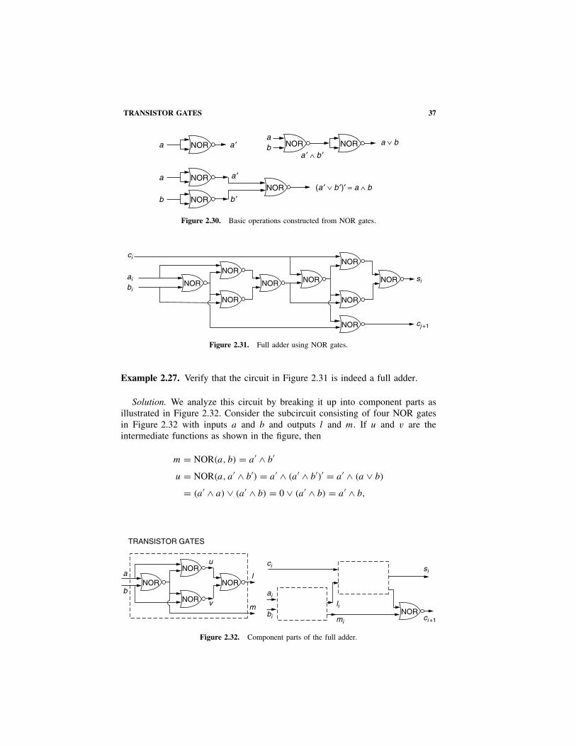
TRANSISTOR GATES 37
aaba ′NOR NORNOR
a a ′NOR(a ′ ∨ b ′)′ = a ∧ b
a ′ ∧ b ′a ∨ b
NOR
b b ′NOR
Figure 2.30. Basic operations constructed from NOR gates.
NOR
NOR
NOR
NOR
NOR
NOR NOR NOR NOR
ci
si
cj +1
ai
bi
Figure 2.31. Full adder using NOR gates.
Example 2.27. Verify that the circuit in Figure 2.31 is indeed a full adder.
Solution. We analyze this circuit by breaking it up into component parts asillustrated in Figure 2.32. Consider the subcircuit consisting of four NOR gatesin Figure 2.32 with inputs a and b and outputs l and m. If u and v are theintermediate functions as shown in the figure, then
m = NOR(a, b) = a′ ∧ b′
u = NOR(a, a′ ∧ b′) = a′ ∧ (a′ ∧ b′)′ = a′ ∧ (a ∨ b)
= (a′ ∧ a) ∨ (a′ ∧ b) = 0 ∨ (a′ ∧ b) = a′ ∧ b,
NOR
NOR
TRANSISTOR GATES
NOR NOR
NOR
a
b
u ci
ai
li
mi
si
ci +1bi
v
l
m
Figure 2.32. Component parts of the full adder.
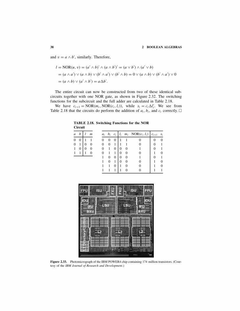
38 2 BOOLEAN ALGEBRAS
and v = a ∧ b′, similarly. Therefore,
l = NOR(u, v) = (a′ ∧ b)′ ∧ (a ∧ b′)′ = (a ∨ b′) ∧ (a′ ∨ b)
= (a ∧ a′) ∨ (a ∧ b) ∨ (b′ ∧ a′) ∨ (b′ ∧ b) = 0 ∨ (a ∧ b) ∨ (b′ ∧ a′) ∨ 0
= (a ∧ b) ∨ (a′ ∧ b′) = a�b′.
The entire circuit can now be constructed from two of these identical sub-circuits together with one NOR gate, as shown in Figure 2.32. The switchingfunctions for the subcircuit and the full adder are calculated in Table 2.18.
We have ci+1 = NOR(mi, NOR(ci, li)), while si = ci�l′i . We see fromTable 2.18 that the circuits do perform the addition of ai, bi , and ci correctly. �
TABLE 2.18. Switching Functions for the NORCircuit
a b l m
0 0 1 10 1 0 01 0 0 01 1 1 0
ai bi ci li mi NOR(ci , li ) ci+1 si
0 0 0 1 1 0 0 00 0 1 1 1 0 0 10 1 0 0 0 1 0 10 1 1 0 0 0 1 01 0 0 0 0 1 0 11 0 1 0 0 0 1 01 1 0 1 0 0 1 01 1 1 1 0 0 1 1
Figure 2.33. Photomicrograph of the IBM POWER4 chip containing 174 million transistors. (Cour-tesy of the IBM Journal of Research and Development.)

REPRESENTATION THEOREM 39
Instead of using many individual transistors, circuits are now made on a singlesemiconductor “chip,” such as the one in Figure 2.33. This chip may containmillions of gates and several layers of semiconductor. Simplification of a circuitmay not mean the reduction of the circuit to the smallest number of gates. Itcould mean simplification to standard modules, or the reduction of the numbersof layers in the chip. In the design of high-speed computers, it is important toreduce the time a circuit will take to perform a given set of operations.
REPRESENTATION THEOREM
A boolean algebra is a generalization of the notion of the algebra of sets. How-ever, we now show that every finite boolean algebra is in fact essentially thesame as the algebra of subsets of some finite set. To be more precise aboutwhat we mean by algebras being essentially the same, we introduce the notionof morphism and isomorphism of boolean algebras. A morphism between twoboolean algebras is a function between their elements that preserves the twobinary operations and the unary operation.
More precisely, if (K, ∧, ∨, ′) and (L, ∩, ∪, −) are two boolean algebras,the function f : K → L is called a boolean algebra morphism if the followingconditions hold for all A,B ∈ K :
(i) f (A ∧ B) = f (A) ∩ f (B).
(ii) f (A ∨ B) = f (A) ∪ f (B).
(iii) f (A′) = f (A).
A boolean algebra isomorphism is a bijective boolean algebra morphism.Isomorphic boolean algebras have identical properties. For example, their poset
diagrams are the same, except for the labeling of the elements. Furthermore, theatoms of one algebra must correspond to the atoms in the isomorphic algebra.
If we wish to find an isomorphism between any boolean algebra, K , and analgebra of sets, the atoms of K must correspond to the singleton elements of thealgebra of sets. This suggests that we try to define an isomorphism from K tothe algebra P (A) of subsets of the set A of atoms of K . The following theoremshows that if K is finite, we can set up such an isomorphism.
Theorem 2.28. Representation Theorem for Finite Boolean Algebras. Let A
be the set of atoms of the finite boolean algebra (K, ∧,∨, ′). Then there is aboolean algebra isomorphism between (K, ∧, ∨, ′) and the algebra of subsets(P (A), ∩, ∪, −).
Proof. We already have a natural correspondence between the atoms of K
and the atoms of P (A). We use the disjunctive normal form (Theorem 2.23) toextend this correspondence to all the elements of K .

40 2 BOOLEAN ALGEBRAS
By the disjunctive normal form, any element of K can be written as a join ofatoms of K , say Bα ∨ · · · ∨ Bω. Define the function f : K → P (A) by
f (Bα ∨ · · · ∨ Bω) = {Bα} ∪ · · · ∪ {Bω}.
The uniqueness of the normal form implies that each element of K has a uniqueimage in P (A) and that f is a bijection.
We still have to show that f is a morphism of boolean algebras. If X andY are two elements of K , the atoms in the normal forms of X ∨ Y and X ∧ Y
are, respectively, the atoms in the forms of X or Y and the atoms common tothe forms of X and Y . Therefore, f (X ∨ Y ) = f (X) ∪ f (Y ), and f (X ∧ Y ) =f (X) ∩ f (Y ). An atom B is in the normal form for X′ if and only if B � X′,which, by Proposition 2.18(iv), happens if and only if B ∧ X = 0. Therefore, theatoms in X′ are all the atoms that are not in X and f (X′) = f (X). This provesthat f is a boolean algebra isomorphism. �
COROLLARY 2.29. If (K, ∧,∨, ′) is a finite boolean algebra, then K has 2n
elements, where n is the number of atoms in K .
Proof. This follows from Theorem 2.5. �
Consider the representation theorem (Theorem 2.28) applied to the booleanalgebra D110, which consists of the divisors of 110. The atoms of this algebraare the prime divisors 2, 5, and 11. Theorem 2.28 defines a boolean algebraisomorphism to the algebra of subsets of {2, 5, 11}. This isomorphism, f , mapsa number onto the subset consisting of its prime divisors; for example, f (11) ={11} and f (10) = {2, 5}.
Example 2.30. Do the divisors of 12 form a boolean algebra under gcd and lcm?
Solution. The set of divisors of 12 is {1, 2, 3, 4, 6, 12}. Since the number ofelements is not a power of 2, it cannot form a boolean algebra. �
Example 2.31. Do the divisors of 24 form a boolean algebra under gcd and lcm?
Solution. There are 8 = 23 divisors of 24, namely 1, 2, 3, 4, 6, 8, 12, and24. However, the poset diagram in Figure 2.34 shows that 2 and 3 are the onlyatoms. Hence, by Corollary 2.29, it cannot be a boolean algebra because it doesnot have 22 = 4 elements. �
An infinite boolean algebra is not necessarily isomorphic to the algebra of allsubsets of a set, but is isomorphic to the algebra of some subsets of a set. Thisresult is known as Stone’s representation theorem, and a proof can be found inMendelson [21, Sec. 5.7].
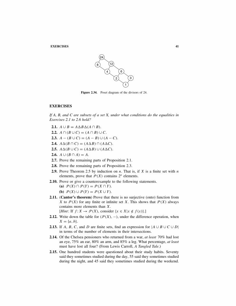
EXERCISES 41
1
3
6
2
4
12
24
8
Figure 2.34. Poset diagram of the divisors of 24.
EXERCISES
If A, B, and C are subsets of a set X, under what conditions do the equalities inExercises 2.1 to 2.6 hold?
2.1. A ∪ B = A�B�(A ∩ B).
2.2. A ∩ (B ∪ C) = (A ∩ B) ∪ C.
2.3. A − (B ∪ C) = (A − B) ∪ (A − C).
2.4. A�(B ∩ C) = (A�B) ∩ (A�C).
2.5. A�(B ∪ C) = (A�B) ∪ (A�C).
2.6. A ∪ (B ∩ A) = A.
2.7. Prove the remaining parts of Proposition 2.1.
2.8. Prove the remaining parts of Proposition 2.3.
2.9. Prove Theorem 2.5 by induction on n. That is, if X is a finite set with n
elements, prove that P (X) contains 2n elements.
2.10. Prove or give a counterexample to the following statements.(a) P (X) ∩ P (Y ) = P (X ∩ Y ).
(b) P (X) ∪ P (Y ) = P (X ∪ Y ).
2.11. (Cantor’s theorem) Prove that there is no surjective (onto) function fromX to P (X) for any finite or infinite set X. This shows that P (X) alwayscontains more elements than X.[Hint : If f : X → P (X), consider {x ∈ X|x /∈ f (x)}.]
2.12. Write down the table for (P (X), −), under the difference operation, whenX = {a, b}.
2.13. If A, B, C, and D are finite sets, find an expression for |A ∪ B ∪ C ∪ D|in terms of the number of elements in their intersections.
2.14. Of the Chelsea pensioners who returned from a war, at least 70% had lostan eye, 75% an ear, 80% an arm, and 85% a leg. What percentage, at leastmust have lost all four? (From Lewis Carroll, A Tangled Tale.)
2.15. One hundred students were questioned about their study habits. Seventysaid they sometimes studied during the day, 55 said they sometimes studiedduring the night, and 45 said they sometimes studied during the weekend.
42 2 BOOLEAN ALGEBRAS
Also, 36 studied during the day and night, 24 during the day and at week-ends, 17 during the night and at weekends, and 3 during the day, night,and weekends. How many did not study at all?
2.16. Prove that the associative laws in defined in the section “Boolean Algebras”follow from the other axioms of a boolean algebra.
2.17. If the zero element is the same as the unit element in a boolean algebra,prove that the algebra has only one element. Is this algebra isomorphic tothe algebra of subsets of some set?
2.18. Draw the poset diagram for F1, the boolean algebra of switching functionsof one variable.
If A, B, and C are elements of a boolean algebra (K, ∧, ∨, ′) and � is the relatedpartial order, prove the assertions in Exercises 2.19 to 2.24 from the axioms andPropositions 2.13, 2.17, and 2.18.
2.19. 0′ = 1.2.20. A ∧ (A′ ∨ B) = A ∧ B.2.21. (A ∧ B) ∨ (B ∧ C) ∨ (C ∧ A) = (A ∨ B) ∧ (B ∨ C) ∧ (C ∨ A).2.22. A � B ∧ C implies that A � B and A � C.2.23. (A ∧ B ′) ∨ C = (B ∧ C) ∨ (B ′ ∧ (A ∨ C)).2.24. A � B if and only if B ′ � A′.2.25. Write down the truth tables for the following propositions. Which of these
propositions are equivalent?(a) A ⇒ B. (b) B ′ ⇒ A′.(c) (A ∧ B) ⇔ B. (d) (A ∨ B) ⇔ A.
2.26. Is the proposition [(A′ ⇒ B) ∧ (B ⇔ C)′] equivalent to [B ∨ (A ∧ C)] or[(C ⇒ B) ∨ (B ⇒ (A ∧ C))]?
2.27. Which of the following are tautologies, and which are contradictions?(a) (A ∧ B) ⇔ (A ⇒ B ′). (b) A ⇒ (B ⇒ A).(c) (A ∧ B ′) ⇔ (A ⇒ B)′. (d) (A ⇒ B) ⇒
((B ⇒ C) ⇒ (A ⇒ C)).2.28. Harry broke the window if and only if he ran away and John was lying.
John said that either Harry broke the window or Harry did not run away.If Harry ran away, then he did not break the window. What conclusionscan you come to?
Draw circuits to realize the expressions in Exercises 2.29 and 2.30.
2.29. (A ∧ (B ∨ C′ ∨ D)) ∨ B ′.2.30. (A ∧ B ′ ∧ C′) ∨ (A′ ∧ B ∧ C) ∨ (A ∧ B ∧ C).2.31. Simplify the following expression and then draw a circuit for it.
((A ∧ B) ∨ C′) ∧ (B ′ ∨ (C ∧ A′)) ∨ (A′ ∧ B ′ ∧ C′).

EXERCISES 43
Give a boolean expression for each of the circuits in Exercises 2.32 to 2.36, findtheir disjunctive normal forms, and then try to simplify the circuits.
2.32.A
AA′
2.33.A
B A′
2.34.A B
C A′
B ′ C
A′ C ′
2.35.A
B B
A′ B ′
A′
2.36.A
C B ′B
B C
A′
A′C ′
2.37. By looking at all the possible paths through the bridge circuit in Figure 2.35,show that it corresponds to the boolean expression
(A ∧ D) ∨ (B ∧ E) ∨ (A ∧ C ∧ E) ∨ (B ∧ C ∧ D).
A
B
CD
E
Figure 2.35
2.38. Find a series-parallel circuit that is equivalent to the bridge circuit inFigure 2.36 and simplify your circuit.
A
BC
CB
A′
Figure 2.36
2.39. A hall light is controlled by two switches, one upstairs and one downstairs.Design a circuit so that the light can be switched on or off from the upstairsor the downstairs.

44 2 BOOLEAN ALGEBRAS
2.40. A large room has three separate entrances, and there is a light switch byeach entrance. Design a circuit that will allow the lights to be turned onor off by throwing any one switch.
2.41. A voting machine for three people contains three YES–NO switches andallows current to pass if and only if there is a majority of YES votes.Design and simplify such a machine.
2.42. Design and simplify a voting machine for five people.2.43. Design a circuit for a light that is controlled by two independent switches
A and B and a master switch C. C must always be able to turn the lighton. When C is off, the light should be able to be turned on and off usingA or B.
2.44. A committee consists of a chairman A, and three other members, B, C,and D. If B, C, and D, are not unanimous in their voting, the chairmandecides the vote. Design a voting machine for this committee and simplifyit as much as possible.
2.45. Verify that the Venn diagram in Figure 2.37 illustrates the 16 atoms for aboolean expression in four variables. Then use the diagram to simplify thecircuit in Figure 2.37.
A
B
C DA
C
B ′
A′
A
D
B
A′
Figure 2.37
2.46. Design four series-parallel circuits to multiply two numbers in binary formthat have at most two digits each.
2.47. Design a circuit that will turn an orange light on if exactly one of the fourswitches A, B, C, and D is on and a green light when all four are on.
2.48. Five switches are set to correspond to a number in binary form that has atmost five digits. Design and simplify a circuit that will switch a light onif and only if the binary number is a perfect square.
2.49. In Chapter 11 we construct a finite field F = {0, 1, α, β} whose multipli-cation table is given in Table 2.19. Writing 00 for 0, 01 for 1, 10 for α,and 11 for β, design and simplify circuits to perform this multiplication.
2.50. A swimming pool has four relay switches that open when the water tem-perature is above the maximum allowable, when the water temperature isbelow the minimum, when the water level is too high, and when the level

EXERCISES 45
TABLE 2.19. Multiplication ina Four-Element Field
· 0 1 α β
0 0 0 0 01 0 1 α β
α 0 α β 1β 0 β 1 α
is too low. These relays are used to control the valves that add cold water,that let water out, and that heat the water in the pool. Design and simplifya circuit that will perform the following tasks. If the temperature is correctbut the level too high, it is to let water out. If the temperature is correct butthe level too low, it is to let in cold water and heat the water. If the pool istoo warm, add cold water and, if the level is also too high, let water out atthe same time. If the pool is too cold but the level correct, heat the water;if the level is too low, heat the water and add cold water, and, if the levelis too high, just let out the water.
2.51. In a dual fashion to the disjunctive normal form, every boolean expressionin n-variables can be written in its conjunctive normal form. What are theconjunctive normal forms for A�B and A ∧ B ′?
Draw poset diagrams for the sets given in Exercises 2.52 to 2.57 with divisi-bility as the partial order and determine whether the systems are lattices orboolean algebras.
2.52. {1, 2, 3, 4, 5, 6}. 2.53. {2, 4, 6, 12}.2.54. D54 2.55. {1, 2, 4, 8}.2.56. D42 2.57. {1, 2, 3, 5, 6, 10, 30, 60}.2.58. Prove that (Dn, |) is a poset for each n � 2, and prove the distributive laws.2.59. Let n = p1p2 · · ·pr , where the pi are distinct primes. Describe the atoms
in the boolean algebra (Dn, gcd, lcm, ′).2.60. Prove that an element A �= 0 in a boolean algebra is an atom if and only
if for each B in the algebra, either A � B or A � B ′.2.61. Suppose that A and B are elements of a boolean algebra. If an element X
in the algebra exists such that A ∧ X = B ∧ X and A ∨ X = B ∨ X, showthat A = B. [Hint : A = A ∧ (A ∨ X).]
2.62. Let K = {x ∈ R|0 � x � 1} and let x ∧ y and x ∨ y be the smaller andlarger of x and y, respectively. Show that it is not possible to define acomplement ′ on K so that (K, ∧, ∨, ′) is a boolean algebra. However,if we define x ′ = 1 − x, which of the properties defined in the section“Boolean Algebras” and in Proposition 2.13 remain true? This is the kindof algebraic model that would be required to deal with transistor switchinggates under transient conditions. The voltage or current varies continuouslybetween the levels 0 and 1, while an AND gate performs the operationx ∧ y, an OR gate performs x ∨ y, and a NOT gate produces x ′.

46 2 BOOLEAN ALGEBRAS
2.63. If f is a boolean algebra morphism from K to L, prove that f (0K) = 0L
and f (1K) = 1L, where 0K, 0L, 1K , and 1L are the respective zero andunit elements.
2.64. Write down the tables for the NOR and NAND operations on the setP ({a, b, c}).
2.65. Can every switching circuit be built out of AND and NOT gates?2.66. (a) Design a half adder using five NOR gates.
(b) Design a half adder using five NAND gates.2.67. Analyze the effect of the circuit in Figure 2.38.
NAND
NOR
a
b
cd
Figure 2.38
2.68. Design a NOR circuit that will produce a parity check symbol for fourbinary input digits; that is, the circuit must produce a 0 if the inputs containan even number of 1’s, and it must produce 1 otherwise.
2.69. One of the basic types of components of a digital computer is a flip-flop.This is a device that can be in one of two states (corresponding to outputs0 and 1) and it will remain in a particular state Q until an input changesthe state to the next state Q∗. One important use of a flip-flop is to storea binary digit. An RS flip-flop is a circuit with two inputs, R and S, andone output, Q, corresponding to the state of the flip-flop. An input R = 1resets the next state Q∗ to 0, and an input S = 1 sets the next state to 1. Ifboth R and S are 0, the next state is the same as the previous state Q. Itis assumed that R and S cannot both be 1 simultaneously. Verify that theNOR circuit in Figure 2.39 is indeed an RS flip-flop. To eliminate spuriouseffects due to the time it takes a transistor to operate, this circuit shouldbe controlled by a “clock.” The output Q should be read only when theclock “ticks,” whereas the inputs are free to change between ticks.
NOR
NOR
S
R Q
Figure 2.39. RS flip-flop.
2.70. A JK flip-flop is similar to an RS flip-flop except that both inputs areallowed to be 1 simultaneously, and in this case the state Q changes to itsopposite state. Design a JK flip-flop using NOR and NAND gates.

3GROUPS
Symmetries and permutations in nature and in mathematics can be describedconveniently by an algebraic object called a group. In Chapter 5, we use grouptheory to determine all the symmetries that can occur in two- or three-dimensionalspace. This can be used, for example, to classify all the forms that chemicalcrystals can take. If we have a large class of objects, some of which are equiva-lent under permutations or symmetries, we show, in Chapter 6, how groups canbe used to count the nonequivalent objects. For example, we count the num-ber of different switching functions of n variables if we allow permutations ofthe inputs.
Historically, the basic ideas of group theory arose with the investigation ofpermutations of finite sets in the theory of equations. One of the aims of mathe-maticians at the beginning of the nineteenth century was to find methods forsolving polynomial equations of degree 5 and higher. Algorithms, involvingthe elementary arithmetical operations and the extraction of roots, were alreadyknown for solving all polynomial equations of degree less than 5; the formulasfor solving quadratic equations had been known since Babylonian times, andcubic and quartic equations had been solved by various Italian mathematiciansin the sixteenth century. However, in 1829, using the rudiments of group theory,the Norwegian Niels Abel (1802–1829) showed that some equations of the fifthdegree could not be solved by any such algorithm. Just before he was mortallywounded in a duel, at the age of 20, the brilliant mathematician Evariste Galois(1811–1832) developed an entire theory that connected the solvability of anequation with the permutation group of its roots. This theory, now called Galoistheory, is beyond the scope of this book, but interested students should look atStewart [35] after reading Chapter 11.
It was not until the 1880s that the abstract definition of a group that weuse today began to emerge. However, Cayley’s theorem, proved at the end ofthis chapter, shows that every abstract group can be considered as a group ofpermutations. It was soon discovered that this concept of a group was so universalthat it cropped up in many different branches of mathematics and science.
Modern Algebra with Applications, Second Edition, by William J. Gilbert and W. Keith NicholsonISBN 0-471-41451-4 Copyright 2004 John Wiley & Sons, Inc.
47

48 3 GROUPS
GROUPS AND SYMMETRIES
A group (G, ·) is a set G together with a binary operation · satisfying thefollowing axioms.
(i) G is closed under the operation ·; that is, a · b ∈ G for all a, b ∈ G.
(ii) The operation · is associative; that is, (a · b) · c = a · (b · c) for alla, b, c ∈ G.
(iii) There is an identity element e ∈ G such that e · a = a · e = a for alla ∈ G.
(iv) Each element a ∈ G has an inverse element a−1 ∈ G such that a−1 · a =a · a−1 = e.
The closure axiom is already implied by the definition of a binary operation;however, it is included because it is often overlooked otherwise.
If the operation is commutative, that is, if a · b = b · a for all a, b ∈ G,the group is called commutative or abelian, in honor of the mathematicianNiels Abel.
Let G be the set of complex numbers {1,−1, i, −i} and let · be the standardmultiplication of complex numbers. Then (G, ·) is an abelian group. The productof any two of these elements is an element of G; thus G is closed under theoperation. Multiplication is associative and commutative in G because multipli-cation of complex numbers is always associative and commutative. The identityelement is 1, and the inverse of each element a is the element 1/a. Hence1−1 = 1, (−1)−1 = −1, i−1 = −i, and (−i)−1 = i. The multiplication of any twoelements of G can be represented by Table 3.1.
The set of all rational numbers, Q, forms an abelian group (Q, +) under addi-tion. The identity is 0, and the inverse of each element is its negative. Similarly,(Z, +), (R, +), and (C, +) are all abelian groups under addition.
If Q∗, R∗, and C∗ denote the set of nonzero rational, real, and complexnumbers, respectively, (Q∗, ·), (R∗, ·), and (C∗, ·) are all abelian groups undermultiplication.
For any set X, (P (X), �) is an abelian group. The group axioms followfrom Proposition 2.3; the empty set, Ø, is the identity, and each element is itsown inverse.
TABLE 3.1. Group{1, −1, i , −i }· 1 −1 i −i
1 1 −1 i −i
−1 −1 1 −i i
i i −i −1 1−i −i i 1 −1

GROUPS AND SYMMETRIES 49
Every group must have at least one element, namely, its identity, e. A groupwith only this one element is called trivial. A trivial group takes the form ({e}, ·),where e · e = e.
Many important groups consist of functions. Given functions f : X → Y andg: Y → Z, their composite g Ž f : X → Z is defined by
(g Ž f )(x) = g(f (x)) for all x ∈ X.
Composition is associative; that is, if h: Z → W , then h Ž (g Ž f ) = (h Ž g) Ž f .Indeed,
(h Ž (g Ž f ))(x) = h(g(f (x))) = ((h Ž g) Ž f )(x)
for all x ∈ X, as is readily verified. In particular, if X is a set, then Ž is anassociative binary operation on the set of all functions f : X → X. Moreover,this operation has an identity: The identity function 1X: X → X is defined by
1X(x) = x for all x ∈ X.
Then 1X Ž f = f = f Ž 1X for all f : X → X. Hence, we say that a functionf ′: X → X is an inverse of f : X → X if
f ′ Ž f = 1X and f Ž f ′ = 1X;
equivalently if f ′(f (x)) = x and f (f ′(x)) = x for all x ∈ X. This inverse isunique when it exists. For if f ′′ is another inverse of f , then
f ′ = f ′ Ž 1X = f ′ Ž (f Ž f ′′) = (f ′ Ž f ) Ž f ′′ = 1X Ž f ′′ = f ′′.
When it exists (see Theorem 3.3) the inverse of f is denoted f −1.
Example 3.1. A translation of the plane R2 in the direction of the vector (a, b)
is a function f : R2 → R2 defined by f (x, y) = (x + a, y + b). The compositionof this translation with a translation g in the direction of (c, d) is the functionf Ž g: R2 → R2, where
f Ž g(x, y) = f (g(x, y)) = f (x + c, y + d) = (x + c + a, y + d + b).
This is a translation in the direction of (c + a, d + b). It can easily be verifiedthat the set of all translations in R2 forms an abelian group, (T(2), Ž ), undercomposition. The identity is the identity transformation 1R2 : R2 → R2, and theinverse of the translation in the direction (a, b) is the translation in the oppositedirection (−a, −b).
A function f : X → Y is called injective or one-to-one if f (x1) = f (x2)
implies that x1 = x2. In other words, an injective function never takes two dif-ferent points to the same point. The function f : X → Y is called surjective or
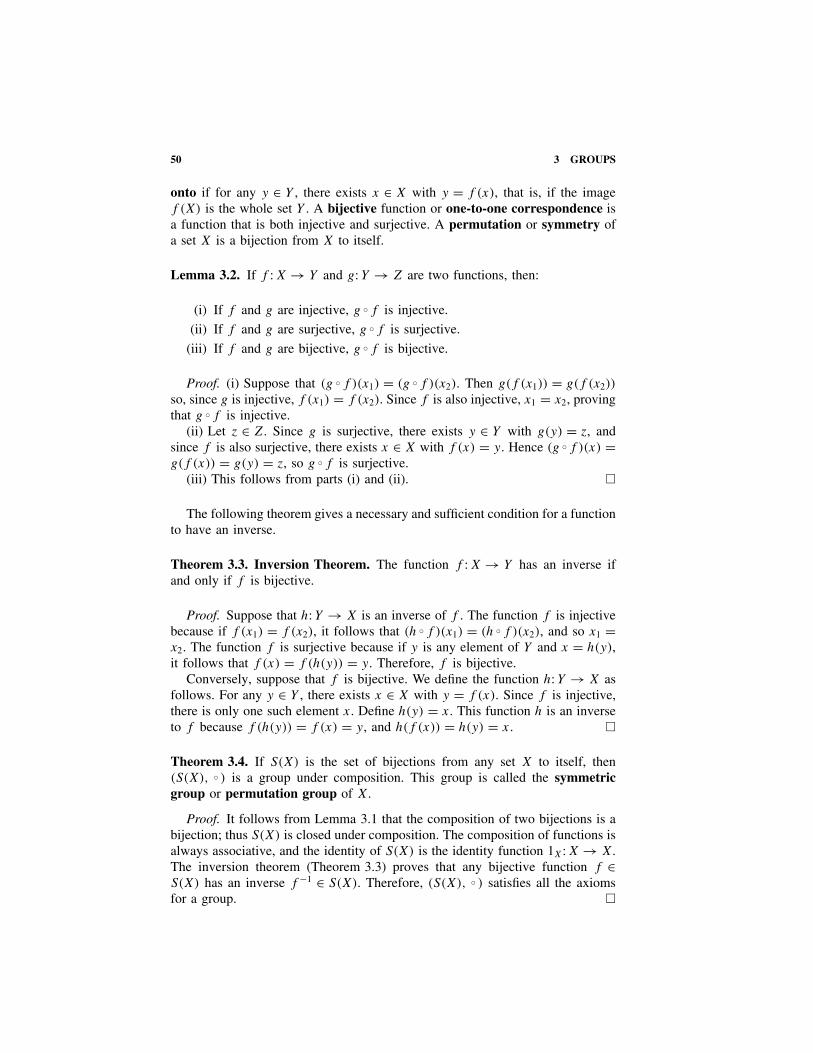
50 3 GROUPS
onto if for any y ∈ Y , there exists x ∈ X with y = f (x), that is, if the imagef (X) is the whole set Y . A bijective function or one-to-one correspondence isa function that is both injective and surjective. A permutation or symmetry ofa set X is a bijection from X to itself.
Lemma 3.2. If f : X → Y and g: Y → Z are two functions, then:
(i) If f and g are injective, g Ž f is injective.
(ii) If f and g are surjective, g Ž f is surjective.
(iii) If f and g are bijective, g Ž f is bijective.
Proof. (i) Suppose that (g Ž f )(x1) = (g Ž f )(x2). Then g(f (x1)) = g(f (x2))
so, since g is injective, f (x1) = f (x2). Since f is also injective, x1 = x2, provingthat g Ž f is injective.
(ii) Let z ∈ Z. Since g is surjective, there exists y ∈ Y with g(y) = z, andsince f is also surjective, there exists x ∈ X with f (x) = y. Hence (g Ž f )(x) =g(f (x)) = g(y) = z, so g Ž f is surjective.
(iii) This follows from parts (i) and (ii). �
The following theorem gives a necessary and sufficient condition for a functionto have an inverse.
Theorem 3.3. Inversion Theorem. The function f : X → Y has an inverse ifand only if f is bijective.
Proof. Suppose that h: Y → X is an inverse of f . The function f is injectivebecause if f (x1) = f (x2), it follows that (h Ž f )(x1) = (h Ž f )(x2), and so x1 =x2. The function f is surjective because if y is any element of Y and x = h(y),it follows that f (x) = f (h(y)) = y. Therefore, f is bijective.
Conversely, suppose that f is bijective. We define the function h: Y → X asfollows. For any y ∈ Y , there exists x ∈ X with y = f (x). Since f is injective,there is only one such element x. Define h(y) = x. This function h is an inverseto f because f (h(y)) = f (x) = y, and h(f (x)) = h(y) = x. �
Theorem 3.4. If S(X) is the set of bijections from any set X to itself, then(S(X), Ž ) is a group under composition. This group is called the symmetricgroup or permutation group of X.
Proof. It follows from Lemma 3.1 that the composition of two bijections is abijection; thus S(X) is closed under composition. The composition of functions isalways associative, and the identity of S(X) is the identity function 1X: X → X.The inversion theorem (Theorem 3.3) proves that any bijective function f ∈S(X) has an inverse f −1 ∈ S(X). Therefore, (S(X), Ž ) satisfies all the axiomsfor a group. �

GROUPS AND SYMMETRIES 51
TABLE 3.2. SymmetryGroup of {a , b}Ž 1X f
1X 1X f
f f 1X
For example, if X = {a, b} is a two-element set, the only bijections from X toitself are the identity 1X and the symmetryf : X → X, defined byf (a) = b, f (b) =a, that interchanges the two elements. The use of the term symmetry to describe thebijection f agrees with one of our everyday uses of the word. In the phrase “theboolean expression (a ∧ b) ∨ (a′ ∧ b′) is symmetrical in a and b” we mean that theexpression is unchanged when we interchange a and b. The symmetric group ofX, S(X) = {1X, f } and its group table is given in Table 3.2. The composition f Ž f
interchanges the two elements a and b twice; thus it is the identity.Since the composition of functions is not generally commutative, S(X) is not
usually an abelian group. Consider the elements f and g in the permutationgroup of {1, 2, 3}, where f (1) = 2, f (2) = 3, f (3) = 1 and g(1) = 1, g(2) =3, g(3) = 2. Then f Ž g(1) = 2, f Ž g(2) = 1, f Ž g(3) = 3, while g Ž f (1) = 3,g Ž f (2) = 2, g Ž f (3) = 1; hence f Ž g �= g Ž f , and S({1, 2, 3}) is not abelian.
A nonsingular linear transformation of the plane is a bijective function of theform f : R2 → R2, where f (x, y) = (a11x + a12y, a21x + a22y) with the deter-minant a11a22 − a12a21 �= 0. It can be verified that the composition of two suchlinear transformations is again of the same type. The set of all nonsingular lineartransformations, L, forms a non-abelian group (L, Ž ).
Besides talking about the symmetries of a distinct set of elements, we oftenrefer, in everyday language, to a geometric object or figure as being symmetrical.We now make this notion more mathematically precise.
If F is a figure in the plane or in space, a symmetry of the figure F orisometry of F is a bijection f : F → F which preserves distances; that is, forall points p, q ∈ F , the distance from f (p) to f (q) must be the same as thedistance from p to q.
One can visualize this operation by imagining F to be a solid object thatcan be picked up and turned in some manner so that it assumes a configurationidentical to the one it had in its original position. For example, the design onthe left of Figure 3.1 has two symmetries: the identity and a half turn about avertical axis, called an axis of symmetry. The design in the center of Figure 3.1
Figure 3.1. Symmetrical designs.

52 3 GROUPS
has three symmetries: the identity and rotations of one-third and two-thirds of arevolution about its center.
However, both the one-third rotation and interchanging two vertices are sym-metries of the equilateral triangle on the right in Figure 3.1, but there is a subtledifference: The rotation can be performed as a physical motion within the planeof the triangle (and so is called a proper symmetry or a proper rotation),while the reflection can only be accomplished as a physical motion by movingthe triangle outside its plane (an improper symmetry or an improper rotation).
The set of all symmetries of a geometric figure forms a group under compo-sition because the composition and inverse of two distance-preserving functionsis distance preserving.
Example 3.5. Write down the table for the group of symmetries of a rectanglewith unequal sides.
Solution. Label the corners of the rectangle 1, 2, 3, and 4 as in Figure 3.2.Any symmetry of the rectangle will send corner points to corner points and sowill permute the corners among themselves. Denote the (improper) symmetryobtained by reflecting the rectangle in the horizontal axis through the center,by a; then a(1) = 4, a(2) = 3, a(3) = 2, and a(4) = 1. This symmetry can alsobe considered as a rotation of the rectangle through half a revolution about thishorizontal axis. There is a similar symmetry, b, about the vertical axis throughthe center. A third (proper) symmetry, c, is obtained by rotating the rectangle inits plane through half a revolution about its center. Finally, the identity map, e,is a symmetry. These are the only symmetries because it can be verified that anyother bijection between the corners will not preserve distances.
The group of symmetries of the rectangle is ({e, a, b, c}, Ž ), and its table, asshown in Table 3.3, can be calculated as follows. The symmetries a, b, and c
are all half turns, so a Ž a, b Ž b, and c Ž c are full turns and are therefore equal tothe identity. The function a Ž b acts on the corner points by a Ž b(1) = a(b(1)) =a(2) = 3, a Ž b(2) = 4, a Ž b(3) = 1, and a Ž b(4) = 2. Therefore, a Ž b = c. Theother products can be calculated similarly. �
This group of symmetries of a rectangle is sometimes called the Klein 4-group, after the German geometer Felix Klein (1849–1925).
We have seen that the group operation can be denoted by various symbols, themost common being multiplication, composition, and addition. It is conventional
b
ac
1 2
4 3
Figure 3.2. Symmetries of a rectangle.

GROUPS AND SYMMETRIES 53
TABLE 3.3. Symmetry Group ofa Rectangle
Ž e a b c
e e a b c
a a e c b
b b c e a
c c b a e
to use addition only for abelian groups. Furthermore, the identity under additionis usually denoted by 0 and the inverse of a by −a. Hence expressions of theform a · b−1 and an = a · · · a, in multiplicative notation, would be written asa − b and na = a + · · · + a, respectively, in additive notation.
In propositions and theorems concerning groups in general, it is conventionalto use multiplicative notation and also to omit the dot in writing a product;therefore, a · b is just written as ab.
Whenever the operation in a group is clearly understood, we denote the groupjust by its underlying set. Therefore, the groups (Z, +), (Q, +), (R, +), and(C, +) are usually denoted just by Z, Q, R, and C, respectively. This shouldcause no confusion because Z, Q, R, and C are not groups under multiplication(since the element 0 has no multiplicative inverse). The symmetric group of X isdenoted just by S(X), the operation of composition being understood. Moreover,if we refer to a group G without explicitly defining the group or the operation,it can be assumed that the operation in G is multiplication.
We now prove two propositions that will enable us to manipulate the elementsof a group more easily. Recall from Proposition 2.10 that the identity of anybinary operation is unique. We first show that the inverse of any element of agroup is unique.
Proposition 3.6. Let � be an associative binary operation on a set S that hasidentity e. Then, if an element a has an inverse, this inverse is unique.
Proof. Suppose that b and c are both inverses of a; thus a � b = b � a = e,and a � c = c � a = e. Now, since e is the identity and � is associative,
b = b � e = b � (a � c) = (b � a) � c = e � c = c.
Hence the inverse of a is unique. �
Note that if ab = e in a group G with identity e, then a−1 = b and b−1 = a.Indeed, b has an inverse b−1 in G, so b−1 = eb−1 = (ab)b−1 = ae = a. Simi-larly, a−1 = b.
Proposition 3.7. If a, b, and c are elements of a group G, then
(i) (a−1)−1 = a.(ii) (ab)−1 = b−1a−1.
(iii) ab = ac or ba = ca implies that b = c. (cancellation law)

54 3 GROUPS
Proof. (i) The inverse of a−1 is an element b such that a−1b = ba−1 = e. Buta is such an element, and by Proposition 3.6 we know that the inverse is unique.Hence (a−1)−1 = a.
(ii) Using associativity, we have
(ab)(b−1a−1) = a((bb−1)a−1) = a(ea−1) = aa−1 = e.
Hence b−1a−1 is the unique inverse of ab.(iii) Suppose that ab = ac. Then a−1(ab) = a−1(ac), so (a−1a)b = (a−1a)c.
That is, eb = ec and b = c. Similarly, ba = ca implies that b = c. �
Notice in part (ii) that the order of multiplication is reversed. This shouldbe familiar from the particular case of the group of invertible n × n matricesunder multiplication. A more everyday example is the operation of putting onsocks and shoes. To reverse the procedure, the shoes are taken off first and thenthe socks.
If a is an element in any group G, we write a1 = a, a2 = aa, a3 = aaa, andso on, just as for numbers. Hence, if k � 1, we define ak to be the product of a
with itself k times. Similarly, we define a−k = (a−1)k for k � 1. Finally, we seta0 to be the identity, again as for numbers. Thus we have defined ak for everyk ∈ Z, and it is a routine verification that the laws of exponents hold:
akam = ak+m, (ak)m = ak+m for all a ∈ G and all k,m ∈ Z.
Moreover:
If ab = ba in G, then (ab)k = akbk for all k ∈ Z.
However, this need not hold if ab �= ba: For example, if a =[
0 −11 0
]and
b =[
1 −11 0
]in the group of invertible 2 × 2 matrices, then (ab)2 �= a2b2.
SUBGROUPS
It often happens that some subset of a group will also form a group under thesame operation. Such a group is called a subgroup. For example, (R, +) is asubgroup of (C, +), and the group of translations of R2 in Example 3.1 is asubgroup of the group of all isometries of R2.
If (G, ·) is a group and H is a nonempty subset of G, then (H, ·) is called asubgroup of (G, ·) if the following conditions hold:
(i) a · b ∈ H for all a, b ∈ H . (closure)(ii) a−1 ∈ H for all a ∈ H . (existence of inverses)

SUBGROUPS 55
Proposition 3.8. If H is a subgroup of (G, ·), then (H, ·) is also a group.
Proof. If H is a subgroup of (G, ·), we show that (H, ·) satisfies all the groupaxioms. The definition above implies that H is closed under the operation; that is,· is a binary operation on H . If a, b, c ∈ H , then (a · b) · c = a · (b · c) in (G, ·)and hence also in (H, ·). Since H is nonempty, it contains at least one element,say h. Now h−1 ∈ H and h · h−1, which is the identity, is in H . The definitionof subgroup implies that (H, ·) contains inverses. Therefore, (H, ·) satisfies allthe axioms of a group. �
Conditions (i) and (ii) are equivalent to the single condition:
(iii) a · b−1 ∈ H for all a, b ∈ H .
However, when H is finite, the following result shows that it is sufficient just tocheck condition (i).
Proposition 3.9. If H is a nonempty finite subset of a group G and ab ∈ H forall a, b ∈ H , then H is a subgroup of G.
Proof. We have to show that for each element a ∈ H , its inverse is alsoin H . All the elements, a, a2 = aa, a3 = aaa, . . . belong to H so, since H isfinite, these cannot all be distinct. Therefore, ai = aj for some 1 � i < j . ByProposition 3.7(iii), we can cancel ai from each side to obtain e = aj−1, wherej − i > 0. Therefore, e ∈ H and this equation can be written as e = a(aj−i−1) =(aj−i−1)a. Hence a−1 = aj−i−1, which belongs to H , since j − i − 1 � 0. �
In the group ({1, −1, i, −i}, ·), the subset {1,−1} forms a subgroup becausethis subset is closed under multiplication. In the group of translations of the plane(Example 3.1), the set of translations in the horizontal direction forms a subgroupbecause compositions and inverses of horizontal translations are still horizontaltranslations.
The group Z is a subgroup of Q, Q is a subgroup of R, and R is a subgroupof C. (Remember that addition is the operation in all these groups.)
However, the set N = {0, 1, 2, . . .} of nonnegative integers is a subset of Z butnot a subgroup, because the inverse of 1, namely, −1, is not in N. This exampleshows that Proposition 3.9 is false if we drop the condition that H be finite.
The relation of being a subgroup is transitive. In fact, for any group G, theinclusion relation between the subgroups of G is a partial order relation.
Example 3.10. Draw the poset diagram of the subgroups of the group of sym-metries of a rectangle.
Solution. By looking at the table of this group in Table 3.3, we see that Ž isa binary operation on {e, a}; thus {e, a} is a subgroup. Also, {e, b} and {e, c} aresubgroups. If a subgroup contains a and b, it must contain a Ž b = c, so it is the

56 3 GROUPS
{e, a, b, c}
{e, c}{e, a} {e, b}
{e}
Figure 3.3. Subgroups of the group of symmetries of a rectangle.
whole group. Similarly, subgroups containing a and c or b and c must be thewhole group. The poset diagram of subgroups is given in Figure 3.3. �
CYCLIC GROUPS AND DIHEDRAL GROUPS
The number of elements in a group G is written |G| and is called the order ofthe group. G is called a finite group if |G| is finite, and G is called an infinitegroup otherwise.
An important class of groups consists of those for which every element can bewritten as a power (positive or negative) of some fixed element. More precisely,a group (G, ·) is called cyclic if there exists an element g ∈ G such that G ={gn|n ∈ Z}. The element g is called a generator of the cyclic group.
Every cyclic group is abelian because gr · gs = gr+s = gs · gr .The group ({1, −1, i, −i}, ·) is a cyclic group of order 4 generated by i because
i0 = 1, i1 = i, i2 = −1, i3 = −i, i4 = 1, i5 = i, and so on. Hence the group canbe written as ({1, i, i2, i3}, ·).
In additive notation, the group (G, +) is cyclic if G = {ng|n ∈ Z} for someg ∈ G. The group (Z, +) is an infinite cyclic group with generator 1 (or −1).
The order of an element g in a group (G, ·) is the least positive integer r
such that gr = e. If no such r exists, the order of the element is said to be infinite.Note the difference between the order of an element and the order of a group.
We are going to find connections between these two orders and later proveLagrange’s theorem, which implies that in a finite group, the order of everyelement divides the order of the group.
For example, in ({1, −1, i, −i}, ·), the identity 1 has order 1, −1 has order 2because (−1)2 = 1, whereas i and −i both have order 4. The group has order 4.
Let Q∗ = Q − {0} be the set of nonzero rational numbers. Then (Q∗, ·) is agroup under multiplication. The order of the identity element 1 is 1, and theorder of −1 is 2. The order of every other element is infinite, because the onlysolutions to qr = 1 with q ∈ Q∗, r � 1 are q = ±1. The group has infinite order.However, it is not cyclic, because there is no rational number r such that everynonzero rational can be written as rn for some n ∈ Z.
The next two results show how the division algorithm for integers (see Appen-dix 2) is used in group theory.
Proposition 3.11. Let a be an element of order r in a group G. Then for k ∈Z, gk = e if and only if r divides k.

CYCLIC GROUPS AND DIHEDRAL GROUPS 57
Proof. If k = rm, m ∈ Z, then ak = (ar)m = em = e. Conversely, if ak = e,write k = qr + s, where q and s are in Z and 0 � s < r . Then as = ak−qr =ak(ar)−q = e · e−q = e. Since 0 � s < r and r is the smallest positive integersuch that ar = e, it follows that s = 0. But then k = qr , as required. �
Proposition 3.12. Every subgroup of a cyclic group is cyclic.
Proof. Suppose that G is cyclic with generator g and that H ⊆ G is a sub-group. If H = {e}, it is cyclic with generator e. Otherwise, let gk ∈ H withk �= 0. Since g−k = (gk)−1 is in H , we have gm ∈ H for some m > 0, and wechoose m to be the smallest such positive integer. Write h = gm; we claim thath generates H . Certainly, hk ∈ H for every k ∈ Z because h ∈ H ; we mustshow that every element a in H is a power of h. Since a ∈ G we have a =gs, s ∈ Z. By the division algorithm, write s = qm + r , where 0 � r < m. Thenar = gs−qm = gs(gm)−q = a · h−q ∈ H , so r = 0 by the choice of m. Hencea = gs = gqm = (gm)q = hq , as we wanted. �
For any element g in a group (G, ·) we can look at all the powers of thiselement, namely, {gr |r ∈ Z}. This may not be the whole group, but it will bea subgroup.
Proposition 3.13. If g is any element of order k in a group (G, ·), then H ={gr |r ∈ Z} is a subgroup of order k in (G, ·). This is called the cyclic subgroupgenerated by g.
Proof. We first check that H is a subgroup of (G, ·). This follows from thefact that gr · gs = gr+s ∈ H and (gr)−1 = g−r ∈ H for all r , s ∈ Z.
If the order of the element g is infinite, we show that the elements gr areall distinct. Suppose that gr = gs , where r > s. Then gr−s = e with r − s > 0,which contradicts the fact that g has infinite order. In this case, |H | is infinite.
If the order of the element g is k, which is finite, we show that H = {g0 =e, g1, g2, . . . , gk−1}. Suppose that gr = gs , where 0 � s < r � k − 1. Multiplyboth sides by g−s so that gr−s = e with 0 < r − s < k. This contradicts the factthat k is the order of g. Hence the elements g0, g1, g2, . . . , gk−1 are all distinct.For any other element, gt , we can write t = qk + r , where 0 � r < k by thedivision algorithm. Hence
gt = gqk+r = (gk)q(gr) = (eq)(gr) = gr .
Hence H = {g0, g1, g2, . . . , gk−1} and |H | = k. �
For example, in (Z, +), the subgroup generated by 3 is {. . . ,−3, 0, 3, 6, 9, . . .},an infinite subgroup that we write as 3Z = {3r|r ∈ Z}.
Theorem 3.14. If the finite group G is of order n and has an element g of ordern, then G is a cyclic group generated by g.

58 3 GROUPS
Proof. From the previous proposition we know that H , the subgroup of G
generated by g, has order n. Therefore, H is a subset of the finite set G withthe same number of elements. Hence G = H and G is a cyclic group gener-ated by g. �
Example 3.15. Show that the Klein 4-group of symmetries of a rectangle, descri-bed in Example 3.5, is not cyclic.
Solution. In the Klein 4-group, the identity has order 1, whereas all the otherelements have order 2. As it has no element of order 4, it cannot be cyclic. �
All the elements of the Klein 4-group can be written in terms of a and b. Wetherefore say that this group can be generated by the two elements a and b.
Example 3.16. Show that the group of proper rotations of a regular n-gon in theplane is a cyclic group of order n generated by a rotation of 2π/n radians. Thisgroup is denoted by Cn.
Solution. This is the group of those symmetries of the regular n-gon that canbe performed in the plane, that is, without turning the n-gon over.
Label the vertices 1 through n as in Figure 3.4. Under any symmetry, thecenter must be fixed, and the vertex 1 can be taken to any of the n vertices. Theimage of 1 determines the rotation; hence the group is of order n.
Let g be the counterclockwise rotation of the n-gon through 2π/n. Theng has order n, and by Theorem 3.14, the group is cyclic of order n. HenceCn = {e, g, g2, . . . , gn−1}. �
Let us now consider the group of all symmetries (both proper and improperrotations) of the regular n-gon. We call this group the dihedral group and denoteit by Dn.
Example 3.17. Show that the dihedral group, Dn, is of order 2n and is not cyclic.
Solution. Label the vertices 1 to n in a counterclockwise direction aroundthe n-gon. Let g be a counterclockwise rotation through 2π/n, and let h be theimproper rotation of the n-gon about an axis through the center and vertex 1, asindicated in Figure 3.5. The element g generates the group Cn, which is a cyclicsubgroup of Dn. The element h has order 2 and generates a subgroup {e, h}.
32
1
n
n − 1
g
g2
Figure 3.4. Elements of Cn.
32
1
n
n − 1
gh
Figure 3.5. Elements of Dn.
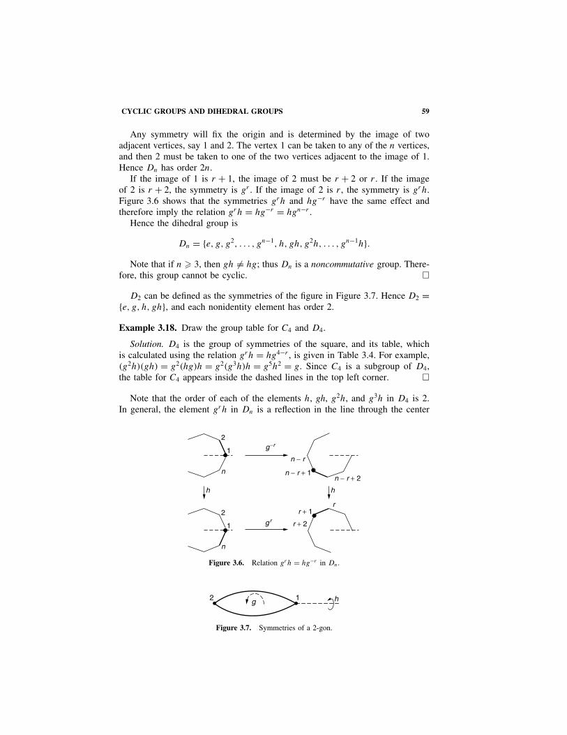
CYCLIC GROUPS AND DIHEDRAL GROUPS 59
Any symmetry will fix the origin and is determined by the image of twoadjacent vertices, say 1 and 2. The vertex 1 can be taken to any of the n vertices,and then 2 must be taken to one of the two vertices adjacent to the image of 1.Hence Dn has order 2n.
If the image of 1 is r + 1, the image of 2 must be r + 2 or r . If the imageof 2 is r + 2, the symmetry is gr . If the image of 2 is r , the symmetry is grh.Figure 3.6 shows that the symmetries grh and hg−r have the same effect andtherefore imply the relation grh = hg−r = hgn−r .
Hence the dihedral group is
Dn = {e, g, g2, . . . , gn−1, h, gh, g2h, . . . , gn−1h}.Note that if n � 3, then gh �= hg; thus Dn is a noncommutative group. There-
fore, this group cannot be cyclic. �
D2 can be defined as the symmetries of the figure in Figure 3.7. Hence D2 ={e, g, h, gh}, and each nonidentity element has order 2.
Example 3.18. Draw the group table for C4 and D4.
Solution. D4 is the group of symmetries of the square, and its table, whichis calculated using the relation grh = hg4−r , is given in Table 3.4. For example,(g2h)(gh) = g2(hg)h = g2(g3h)h = g5h2 = g. Since C4 is a subgroup of D4,the table for C4 appears inside the dashed lines in the top left corner. �
Note that the order of each of the elements h, gh, g2h, and g3h in D4 is 2.In general, the element grh in Dn is a reflection in the line through the center
h h
2
n
1
2
n
1
g−r
g r
n − r
n − r + 1n − r + 2
r + 2
r + 1r
Figure 3.6. Relation grh = hg−r in Dn.
h12 g
Figure 3.7. Symmetries of a 2-gon.

60 3 GROUPS
TABLE 3.4. Group D4
• e g g2 g3 h gh g2h g 3h
e e g g2 g3 h gh g2h g 3hg g g2 g3 e gh g2h g 3h hg2 g2 g3 e g g2h g 3h h ghg3 g3 e g g2 g3h h gh g2hh h g 3h g 2h gh e g3 g2 ggh gh h g 3h g 2h g e g3 g2
g2h g2h gh h g 3h g 2 g e g3
g3h g3h g 2h gh h g 3 g2 g e
of the n-gon bisecting the angle between vertices 1 and r + 1. Therefore, grh
always has order 2.
MORPHISMS
Recall that a morphism between two algebraic structures is a function that pre-serves their operations. For instance, in Example 3.5, each element of the groupK of symmetries of the rectangle induces a permutation of the vertices 1, 2, 3,4. This defines a function f : K → S({1, 2, 3, 4}) with the property that the com-position of two symmetries of the rectangle corresponds to the composition ofpermutations of the set {1, 2, 3, 4}. Since this function preserves the operations,it is a morphism of groups.
Two groups are isomorphic if their structures are essentially the same. Forexample, the group tables of the cyclic group C4 and ({1, −1, i, −i}, ·) would beidentical if we replaced a rotation through nπ/2 by in. We would therefore saythat (C4, Ž ) and ({1, −1, i, −1}, ·) are isomorphic.
If (G, ·) and (H, ·) are two groups, the function f : G → H is called a groupmorphism if
f (a · b) = f (a) · f (b) for all a, b ∈ G.
If the groups have different operations, say they are (G, ·) and (H, �), the con-dition would be written as
f (a · b) = f (a) � f (b).
We often use the notation f : (G, ·) → (H, �) for such a morphism. Many authorsuse homomorphism instead of morphism but we prefer the simpler terminology.
A group isomorphism is a bijective group morphism. If there is an isomor-phism between the groups (G, ·) and (H, �), we say that (G, ·) and (H, �) areisomorphic and write (G, ·) ∼= (H, �).
If G and H are any two groups, the trivial function that maps every elementof G to the identity of H is always a morphism. If i: Z → Q is the inclusionmap, i is a group morphism from (Z, +) to (Q, +). In fact, if H is a subgroupof G, the inclusion map H → G is always a group morphism.

MORPHISMS 61
Let f : Z → {1, −1} be the function defined by f (n) = 1 if n is even, andf (n) = −1 if n is odd. Then it can be verified that f (m + n) = f (m) · f (n) forany m, n ∈ Z, so this defines a group morphism f : (Z, +) → ({1, −1}, ·).
Let GL(2, R) be the set of 2 × 2 invertible real matrices. The one-to-onecorrespondence between the set, L, of invertible linear transformations of theplane and the 2 × 2 coefficient matrices is an isomorphism between the groups(L, Ž ) and (GL(2, R), ·).
Isomorphic groups share exactly the same properties, and we sometimes iden-tify the groups via the isomorphism and give them the same name. If f : G → H
is an isomorphism between finite groups, the group table of H is the same asthat of G, when each element g ∈ G is replaced by f (g) ∈ H .
Besides preserving the operations of a group, the following result shows thatmorphisms also preserve the identity and inverses.
Proposition 3.19. Let f : G → H be a group morphism, and let eG and eH bethe identities of G and H , respectively. Then
(i) f (eG) = eH .(ii) f (a−1) = f (a)−1 for all a ∈ G.
Proof. (i) Since f is a morphism, f (eG)f (eG) = f (eG · eG) = f (eG) =f (eG)eH . Hence (i) follows by cancellation in H (Proposition 3.7).
(ii) f (a) · f (a−1) = f (a · a−1) = f (eG) = eH by (i). Hence f (a−1) is theunique inverse of f (a); that is f (a−1) = f (a)−1. �
Theorem 3.20. Cyclic groups of the same order are isomorphic.
Proof. Let G = {gr |r ∈ Z} and H = {hr |r ∈ Z} be cyclic groups. If G andH are infinite, then g has infinite order, so for r, s ∈ Z, gr = gs if and only ifr = s (see Proposition 3.13). Hence the function f : G → H defined by f (gr) =hr, r ∈ Z, is a bijection, and
f (grgs) = f (gr+s) = hr+s = hrhs = f (gr)f (gs)
for all r, s ∈ Z, so f is a group isomorphism.If |G| = n = |H |, then G = {e, g, g2, . . . , gn−1}, where these powers of
g are all distinct (see the proof of Proposition 3.13). Similarly, H ={e, h, h2, . . . , hn−1}. Then the function f : G → H defined by f (gr) = hr , isagain a bijection. To see that it is a morphism, suppose that 0 � r, s � n − 1,and let r + s = kn + l, where 0 � l � n − 1. Then
f (gr · gs) = f (gr+s) = f (gkn+l) = f ((gn)k · gl) = f (ek · gl) = f (gl) = hl
and
f (gr) · f (gs) = hr · hs = hr+s = hkn+l = (hn)k · hl = ek · hl = hl,
so f is an isomorphism. �

62 3 GROUPS
Hence every cyclic group is isomorphic to either (Z, +) or (Cn, ·) for some n.In the next chapter, we see that another important class of cyclic groups consistsof the integers modulo n, (Zn,+). Of course, the theorem above implies that(Zn,+) ∼= (Cn, ·).
Any morphism, f : G → H , from a cyclic group G to any group H is deter-mined just by the image of a generator. If g generates G and f (g) = h, it followsfrom the definition of a morphism that f (gr) = f (g)r = hr for all r ∈ Z.
Proposition 3.21. Corresponding elements under a group isomorphism have thesame order.
Proof. Let f : G → H be an isomorphism, and let f (g) = h. Suppose that g
and h have orders m and n, respectively, where m is finite. Then hm = f (g)m =f (gm) = f (e) = e. So n is also finite, and n � m, since n is the least positiveinteger with the property hn = e.
On the other hand, if n is finite then f (gn) = f (g)n = hn = e = f (e). Sincef is bijective, gn = e, and hence m is finite and m � n.
Therefore, either m and n are both finite and m = n, or m and n are bothinfinite. �
Example 3.22. Is D2 isomorphic to C4 or the Klein 4-group of symmetries ofa rectangle?
Solution. Compare the orders of the elements given in Table 3.5. By Propo-sition 3.21 we see that D2 cannot be isomorphic to C4 but could possibly beisomorphic to the Klein 4-group.
In the Klein 4-group we can write c = a Ž b and we can obtain a bijection, f ,from D2 to the Klein 4-group, by defining f (g) = a and f (h) = b. Table 3.6for the two groups show that this is an isomorphism. �
TABLE 3.5
D2 C4 Klein 4-Group
Element Order Element Order Element Order
e 1 e 1 e 1g 2 g 4 a 2h 2 g2 2 b 2gh 2 g3 4 c 2
TABLE 3.6. Isomorphic Groups
Group D2 Klein 4-Group
· e g h gh Ž e a b c
e e g h gh e e a b c
g g e gh h a a e c b
h h gh e g b b c e a
gh gh h g e c c b a e

PERMUTATION GROUPS 63
PERMUTATION GROUPS
A permutation of n elements is a bijective function from the set of the n elementsto itself. The permutation groups of two sets, with the same number of elements,are isomorphic. We denote the permutation group of X = {1, 2, 3, . . . , n} by(Sn, Ž ) and call it the symmetric group on n elements. Hence Sn
∼= S(Y ) forany n element set Y .
Proposition 3.23. |Sn| = n!
Proof. The order of Sn is the number of bijections from {1, 2, . . . , n} to itself.There are n possible choices for the image of 1 under a bijection. Once theimage of 1 has been chosen, there are n − 1 choices for the image of 2. Thenthere are n − 2 choices for the image of 3. Continuing in this way, we see that|Sn| = n(n − 1)(n − 2) · · · 2 · 1 = n! �
If π : {1, 2, . . . , n} → {1, 2, . . . , n} is a permutation, we denote it by(
1 2 · · · nπ(1) π(2) · · · π(n)
).
For example, the permutation of {1, 2, 3} that interchanges 1 and 3 is written(1 2 33 2 1
). We think of this as
1 2 3
↓ ↓ ↓3 2 1
.
We can write S2 ={(
1 21 2
),
(1 22 1
)}, which has two elements and
S3 ={(
1 2 31 2 3
),
(1 2 33 1 2
),
(1 2 32 3 1
),
(1 2 31 3 2
),
(1 2 32 1 3
),
(1 2 33 2 1
)},
which is of order 3! = 6.If π, ρ ∈ Sn are two permutations, their product π Ž ρ is the permutation obtai-
ned by applying ρ first and then π . This agrees with our notion of composition offunctions because (π Ž ρ)(x) = π(ρ(x)). (However, the reader should be awarethat some authors use the opposite convention in which π is applied first andthen ρ.)
Example 3.24. If π =(
1 2 33 1 2
)and ρ =
(1 2 33 2 1
)are two elements of
S3, calculate π Ž ρ and ρ Ž π .
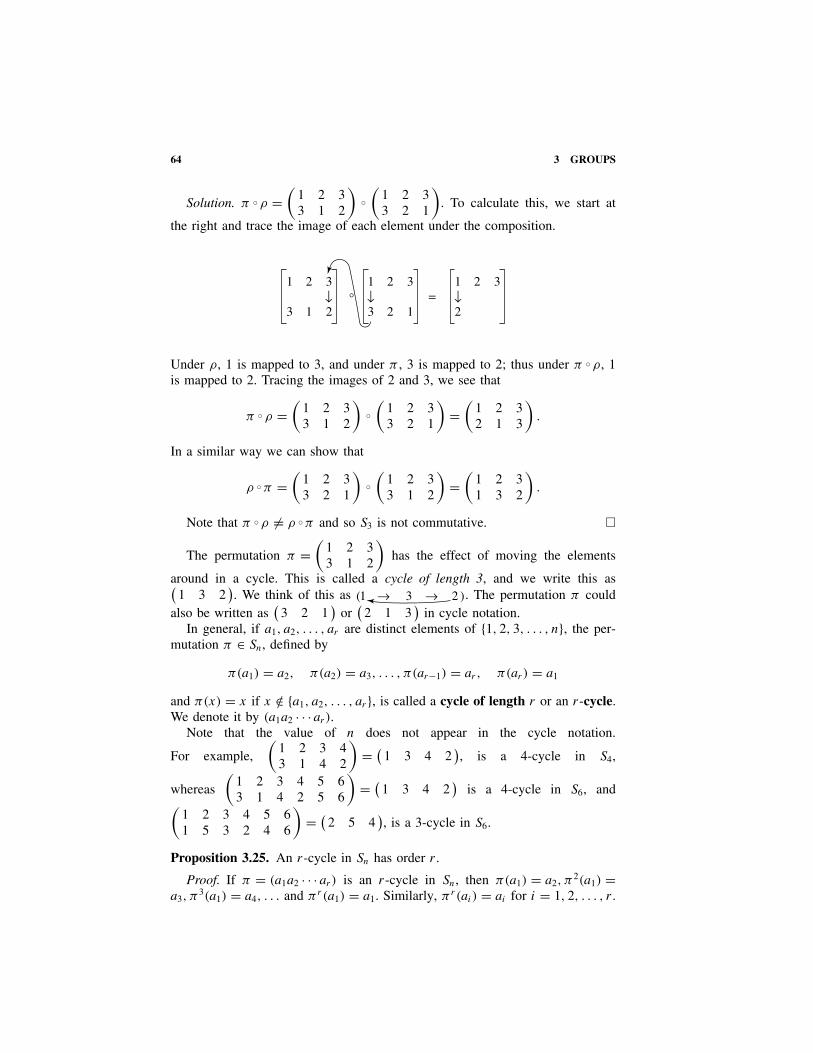
64 3 GROUPS
Solution. π Ž ρ =(
1 2 33 1 2
)Ž
(1 2 33 2 1
). To calculate this, we start at
the right and trace the image of each element under the composition.
1 2 3
3 1 2
1 2 3
3 2 1=
1 2 3
2↓ ↓ ↓°
Under ρ, 1 is mapped to 3, and under π , 3 is mapped to 2; thus under π Ž ρ, 1is mapped to 2. Tracing the images of 2 and 3, we see that
π Ž ρ =(
1 2 33 1 2
)Ž
(1 2 33 2 1
)=
(1 2 32 1 3
).
In a similar way we can show that
ρ Ž π =(
1 2 33 2 1
)Ž
(1 2 33 1 2
)=
(1 2 31 3 2
).
Note that π Ž ρ �= ρ Ž π and so S3 is not commutative. �
The permutation π =(
1 2 33 1 2
)has the effect of moving the elements
around in a cycle. This is called a cycle of length 3, and we write this as(1 3 2
). We think of this as 1 3 2( )→ → . The permutation π could
also be written as(
3 2 1)
or(
2 1 3)
in cycle notation.In general, if a1, a2, . . . , ar are distinct elements of {1, 2, 3, . . . , n}, the per-
mutation π ∈ Sn, defined by
π(a1) = a2, π(a2) = a3, . . . , π(ar−1) = ar, π(ar) = a1
and π(x) = x if x /∈ {a1, a2, . . . , ar}, is called a cycle of length r or an r-cycle.We denote it by (a1a2 · · · ar).
Note that the value of n does not appear in the cycle notation.
For example,
(1 2 3 43 1 4 2
)= (
1 3 4 2), is a 4-cycle in S4,
whereas
(1 2 3 4 5 63 1 4 2 5 6
)= (
1 3 4 2)
is a 4-cycle in S6, and(1 2 3 4 5 61 5 3 2 4 6
)= (
2 5 4), is a 3-cycle in S6.
Proposition 3.25. An r-cycle in Sn has order r .
Proof. If π = (a1a2 · · · ar) is an r-cycle in Sn, then π(a1) = a2, π2(a1) =
a3, π3(a1) = a4, . . . and πr(a1) = a1. Similarly, πr(ai) = ai for i = 1, 2, . . . , r .

PERMUTATION GROUPS 65
Since πr fixes all the other elements, it is the identity permutation. But noneof the permutations π, π2, . . . , πr−1 equal the identity permutation because theyall move the element a1. Hence the order of π is r . �
Example 3.26. Write down π = (1 3 4 2
), ρ = (
1 3), and σ =(
1 2)
Ž(
3 4)
as permutations in S4. Calculate π Ž ρ Ž σ .
Solution.
(1 3 4 2
) =(
1 2 3 43 1 4 2
),
(1 3
) =(
1 2 3 43 2 1 4
),
(1 2
)Ž
(3 4
) =(
1 2 3 42 1 4 3
).
We can either calculate a product of cycles from the permutation representationor we can use the cycle representation directly. Let us calculate π Ž ρ Ž σ fromtheir cycles. Remember that a cycle in S4 is a bijection from {1, 2, 3, 4} to itself,and a product of cycles is a composition of functions. In calculating such acomposition, we begin at the right and work our way left. Consider the effect ofπ Ž ρ Ž σ on each of the elements 1, 2, 3, and 4.
π Ž ρ Ž σ = (1 3 4 2
)Ž
(1 3
)Ž
(1 2
)Ž
(3 4
)1 ←−−−−−−− 2 ←− 2 ←− 1 ←− 1
4 ←−−−−−−− 3 ←− 1 ←− 2 ←− 2
2 ←−−−−−−− 4 ←− 4 ←− 4 ←− 3
3 ←−−−−−−− 1 ←− 3 ←− 3 ←− 4
For example, 2 is left unchanged by(
3 4); then 2 is sent to 1 under
(1 2
),
1 is sent to 3 under(
1 3), and finally, 3 is sent to 4 under
(1 3 4 2
).
Hence π Ž ρ Ž σ sends 2 to 4. The permutation π Ž ρ Ž σ also sends 4 to 3, 3 to 2,and fixes 1. Therefore, π Ž ρ Ž σ = (
2 4 3). �
Permutations that are not cycles can be split up into two or more cycles asfollows. If π is a permutation in Sn and a ∈ {1, 2, 3, . . . , n}, the orbit of a
under π consists of the distinct elements a, π(a), π2(a), π3(a), . . .. We can splita permutation up into its different orbits, and each orbit will give rise to a cycle.
Consider the permutation π =(
1 2 3 4 5 6 7 83 2 8 1 5 7 6 4
)∈ S8. Here
π(1) = 3, π2(1) = π(3) = 8, π3(1) = 4, and π4(1) = 1; thus the orbit of 1 is{1, 3, 8, 4}. This is also the orbit of 3, 4, and 8. This orbit gives rise to the cycle(
1 3 8 4). Since π leaves 2 and 5 fixed, their orbits are {2} and {5}. The
orbit of 6 and 7 is {6, 7}, which gives rise to the 2-cycle(
6 7). We can picture
the orbits and their corresponding cycles as in Figure 3.8.

66 3 GROUPS
2 6
7
5
1
8
34
Figure 3.8. Disjoint cycle decomposition.
It can be verified that π = (1 3 8 4
)Ž (2) Ž (5) Ž
(6 7
). Since no num-
ber is in two different cycles, these cycles are called disjoint. If a permutationis written as a product of disjoint cycles, it does not matter in which orderwe write the cycles. We could write π = (5) Ž
(6 7
)Ž (2) Ž
(1 3 8 4
).
When writing down a product of cycles, we often omit the 1-cycles and writeπ = (
1 3 8 4)
Ž(
6 7). The identity permutation is usually just written
as (1).
Proposition 3.27. Every permutation can be written as a product of disjointcycles.
Proof. Let π be a permutation and let γ1, . . . , γk be the cycles obtained asdescribed above from the orbits of π . Let a1 be any number in the domainof π , and let π(a1) = a2. If γi is the cycle containing a1, we can write γi =(a1a2 · · · ar); the other cycles will not contain any of the elements a1, a2, . . . , ar
and hence will leave them all fixed. Therefore, the product γ1 Ž γ2 Ž · · · Ž γk
will map a1 to a2, because the only cycle to move a1 or a2 is γi . Henceπ = γ1 Ž γ2 Ž · · · Ž γk , because they both have the same effect on all the numbersin the domain of π . �
Corollary 3.28. The order of a permutation is the least common multiple of thelengths of its disjoint cycles.
Proof. If π is written in terms of disjoint cycles as γ1 Ž γ2 Ž · · · Ž γk , the orderof the cycles can be changed because they are disjoint. Therefore, for any integerm, γ m = γ m
1Ž γ m
2Ž · · · Ž γ m
k . Because the cycles are disjoint, this is the identityif and only if γ m
i is the identity for each i. The least such integer is the leastcommon multiple of the orders of the cycles. �
Example 3.29. Find the order of the permutation
π =(
1 2 3 4 5 6 7 83 5 8 7 1 4 6 2
).
Solution. We can write this permutation in terms of disjoint cycles as
π = (1 3 8 2 5
)Ž
(4 7 6
).
Hence the order of π is lcm (5, 3) = 15. Of course, we could calculateπ2, π3, π4, . . . until we obtained the identity, but this would take muchlonger. �

EVEN AND ODD PERMUTATIONS 67
1
2 3
1
2 3
1
2 3
1
2 3
1
2 3
1
2 3
1 2 31 2 3
= (1) = e 1 2 32 3 1
= (1 2 3) = g
1 2 31 3 2
= (2 3) = h 1 2 32 1 3
= (1 2) = gh 1 2 33 2 1
= (1 3) = g2h
1 2 33 1 2
= (1 3 2) = g2
Figure 3.9. Symmetries of an equilateral triangle.
TABLE 3.7. Group S3
Ž (1) (123) (132) (23) (12) (13)
(1) (1) (123) (132) (23) (12) (13)(123) (123) (132) (1) (12) (13) (23)(132) (132) (1) (123) (13) (23) (12)(23) (23) (13) (12) (1) (132) (123)(12) (12) (23) (13) (123) (1) (132)(13) (13) (12) (23) (132) (123) (1)
Example 3.30. Show that D3 is isomorphic to S3 and write out the table for thelatter group.
Solution. D3 is the group of symmetries of an equilateral triangle, and anysymmetry induces a permutation of the vertices. This defines a function f : D3 →S3. If σ, τ ∈ D3, then f (σ Ž τ) is the induced permutation on the vertices, whichis the same as f (σ) Ž f (τ). Hence f is a morphism. Figure 3.9 illustrates the sixelements of D3 and their corresponding permutations. We shade the undersideof the triangle and mark the corner near vertex 1 to illustrate how the trianglemoves. To visualize this, imagine a triangular jigsaw puzzle piece and considerall possible ways of fitting this piece into a triangular hole. Any proper rotationwill leave the white side uppermost, whereas an improper rotation will leave theshaded side uppermost.
The six permutations are all distinct; thus f is a bijection and an isomorphismbetween D3 and S3. The group table for S3 is given in Table 3.7. �
EVEN AND ODD PERMUTATIONS
We are going to show that every permutation can be given a parity, even orodd. The definition derives from an action of each permutation σ in Sn on a

68 3 GROUPS
polynomial f (x1, x2, . . . , xn) in n variables by permuting the variables:
σf (x1, x2, . . . , xn) = f (xσ1, xσ2, . . . , xσn).
For example, if σ = (1 2 3
)in S4 and f (x1, x2, x3, x4) = 2x1x4 − 3x2
2 +x2x
33 , then σf = 2x2x4 − 3x2
3 + x3x31 .
Our use of this action involves a particular polynomial D = D(x1, x2, . . . , xn)
called the discriminant, defined to be the product of all terms (xi − xj ), wherei < j . More formally,
D =∏
0�i<j�n
(xi − xj ).
For example, if n = 3, then D = (x1 − x2)(x1 − x3)(x2 − x3). Given a permuta-tion σ ∈ Sn, we have
σD =∏
0�i<j�n
(xσi − xσj ).
Thus if n = 3 and σ = (12) ∈ S3, then σD = (x2 − x1)(x2 − x3)(x1 − x3) =−D. In fact, σD = ±D for every σ ∈ Sn, and we say that
σ is even if σD = D and σ is odd if σD = −D.
We are going to determine an easy method for deciding which is the case. A 2-cycle is called a transposition, and surprisingly, much of the discussion centersaround determining the parity of these transpositions. We are going to show thatevery transposition is odd.
Let D denote the discriminant in n variables x1, x2, . . . , xn, and define
Dk/m = the product of all terms in D involving xk, except (xk − xm)
Dk,m = the product of all terms in D involving neither xk nor xm.
For example, if n = 5, we have
D2/4 = (x1 − x2)(x2 − x3)(x2 − x5)
D4/2 = (x1 − x4)(x3 − x4)(x4 − x5)
D2,4 = (x1 − x3)(x1 − x5)(x3 − x5).
Then D factors as follows:
D = (xk − xm)Dk/mDm/kDk,m.
Now fix a transposition τ = (k m) in Sn, where k < m. Since τ interchanges k
and m, we see that
τDk/m = uDm/k where u = 1 or u = −1.
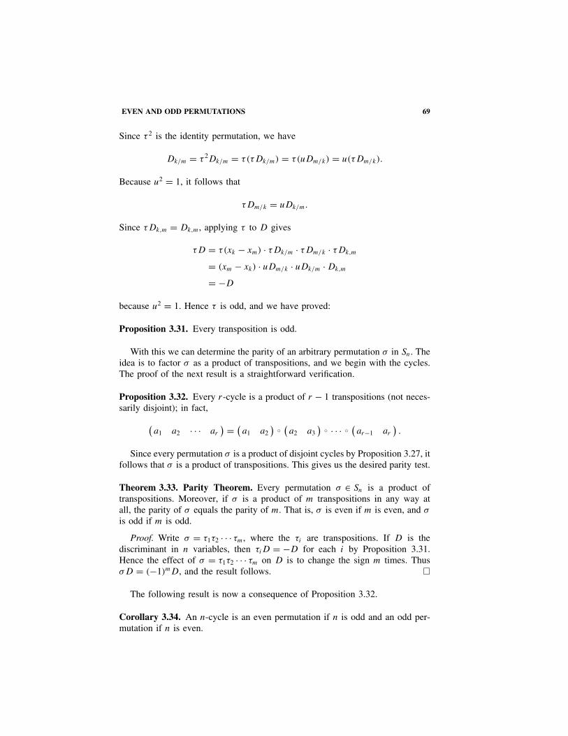
EVEN AND ODD PERMUTATIONS 69
Since τ 2 is the identity permutation, we have
Dk/m = τ 2Dk/m = τ(τDk/m) = τ(uDm/k) = u(τDm/k).
Because u2 = 1, it follows that
τDm/k = uDk/m.
Since τDk,m = Dk,m, applying τ to D gives
τD = τ(xk − xm) · τDk/m · τDm/k · τDk,m
= (xm − xk) · uDm/k · uDk/m · Dk,m
= −D
because u2 = 1. Hence τ is odd, and we have proved:
Proposition 3.31. Every transposition is odd.
With this we can determine the parity of an arbitrary permutation σ in Sn. Theidea is to factor σ as a product of transpositions, and we begin with the cycles.The proof of the next result is a straightforward verification.
Proposition 3.32. Every r-cycle is a product of r − 1 transpositions (not neces-sarily disjoint); in fact,
(a1 a2 · · · ar
) = (a1 a2
)Ž
(a2 a3
)Ž · · · Ž
(ar−1 ar
).
Since every permutation σ is a product of disjoint cycles by Proposition 3.27, itfollows that σ is a product of transpositions. This gives us the desired parity test.
Theorem 3.33. Parity Theorem. Every permutation σ ∈ Sn is a product oftranspositions. Moreover, if σ is a product of m transpositions in any way atall, the parity of σ equals the parity of m. That is, σ is even if m is even, and σ
is odd if m is odd.
Proof. Write σ = τ1τ2 · · · τm, where the τi are transpositions. If D is thediscriminant in n variables, then τiD = −D for each i by Proposition 3.31.Hence the effect of σ = τ1τ2 · · · τm on D is to change the sign m times. ThusσD = (−1)mD, and the result follows. �
The following result is now a consequence of Proposition 3.32.
Corollary 3.34. An n-cycle is an even permutation if n is odd and an odd per-mutation if n is even.

70 3 GROUPS
Example 3.35. Write the permutation
π =(
1 2 3 4 5 6 7 84 1 8 2 7 3 6 5
)
as a product of disjoint cycles and determine its order and parity.
Solution. As disjoint cycles π = (1 4 2
)Ž
(3 8 5 7 6
). Hence the
order of π is lcm (3, 5) = 15. The parity of the 3-cycle(
1 4 2)
is even, andthe parity of the 5-cycle
(3 8 5 7 6
)is even; therefore, the parity of π is
(even ) Ž (even ) = even. �
Denote the set of even permutations on n elements by An. It follows fromTheorem 3.33 that An is a subgroup of Sn, called the alternating group on n
elements. For example,
A4 =
(1 2) Ž (3 4),
(1), (1 3) Ž (2 4),(1 2 3), (1 2 4), (1 3 4), (2 3 4),
(1 4) Ž (2 3),(1 3 2), (1 4 2), (1 4 3), (2 4 3),
,
a group of 12 elements. In fact, we have
Theorem 3.36. |An| = 12n! for every n � 2.
Proof. Let On denote the set of odd permutations in Sn, so that Sn = An ∪ On
and An ∩ On = Ø. Hence n! = |Sn| = |An| + |On|, so it suffices to show that|An| = |On|. We do this by finding a bijection f : An → On. To this end, writeτ = (
1 2)
and define f by f (σ) = τ Ž σ for all σ in An (τ Ž σ is odd becauseσ is even and τ is odd). Then f is injective because f (σ) = f (σ1) implies thatτ Ž σ = τ Ž σ1, so σ = σ1 by cancellation in Sn. To see that f is surjective, letλ ∈ On. Then τ Ž λ ∈ An and f (τ Ž λ) = τ Ž (τ Ž λ) = λ because τ Ž τ = ε. Thusf is surjective, as required. �
Proposition 3.37. Every even permutation can be written as a product of 3-cycles(not necessarily disjoint).
Proof. By Theorem 3.33, an even permutation can be written as a product ofan even number of transpositions. We show that any product of two transpositionsis a product of 3-cycles. If these two transpositions are identical, their productis the identity. If the two transpositions have one element in common, say (ab)and (bc), their product (ab) Ž (bc) = (abc), a 3-cycle. If the two transpositionshave no elements in common, say (ab) and (cd ), we can write their product as
(ab) Ž (cd) = (ab) Ž (bc) Ž (bc) Ž (cd) = (abc) Ž (bcd),
a product of two 3-cycles. �

EXERCISES 71
Theorem 3.33 and Proposition 3.37 show, respectively, that Sn is generatedby the 2-cycles and An is generated by the 3-cycles.
CAYLEY’S REPRESENTATION THEOREM
At the beginning of the nineteenth century, groups appeared only in a veryconcrete form, such as symmetry groups or permutation groups. Arthur Cayley(1821–1895) was the first mathematician to deal with groups abstractly in termsof axioms, but he showed that any abstract group can be considered as a subgroupof a symmetric group. Hence, in some sense, if you know all about symmetrygroups and permutation groups, you know all about group theory. This result isanalogous to Stone’s representation theorem for boolean algebras, which provesthat any abstract boolean algebra can be considered as an algebra of subsets ofa set.
Theorem 3.38. Cayley’s Theorem. Every group (G, ·) is isomorphic to a sub-group of its symmetric group (S(G), Ž ).
Proof. For each element g ∈ G, define πg: G → G by πg(x) = g · x. We showthat πg is a bijection. It is surjective because, for any y ∈ G, πg(g
−1 · y) = g ·(g−1 · y) = y. It is injective because πg(x) = πg(y) implies that g · x = g · y,and so, by Proposition 3.7, x = y. Hence πg ∈ S(G).
Let H = {πg ∈ S(G)|g ∈ G}. We show that (H, Ž ) is a subgroup of (S(G), Ž )
isomorphic to (G, ·). In fact, we show that the function ψ : G → H by ψ(g) = πg
is a group isomorphism. This is clearly surjective. It is also injective becauseψ(g) = ψ(h) implies that πg = πh, and πg(e) = πh(e) implies that g = h.
It remains to show that ψ preserves the group operation. If g, h ∈G, πg·h(x) = (g · h)(x) = g · (h · x) = πg(h · x) = (πg Ž πh)(x) and πg·h = πg Žπh. Also, πh−1 Ž πh = πh−1·h = πe; thus (πh)
−1 = πh−1 ∈ H . Hence H is asubgroup of S(G), and ψ(g · h) = ψ(g) Ž ψ(h). �
Corollary 3.39. If G is a finite group of order n, then G is isomorphic to asubgroup of Sn.
Proof. This follows because S(G) is isomorphic to Sn. �
This is not of very much practical value, however, because Sn has order n!,which is much larger than the order of G, in general.
EXERCISES
Construct tables for the groups designated in Exercises 3.1 to 3.4.
3.1. C5. 3.2 D4.
3.3. (P (X), �), where X = {a, b, c}. 3.4 A4.

72 3 GROUPS
For Exercises 3.5 to 3.16, state which are groups and which are abelian groups.Give reasons for your answers.
3.5. (Mn(R), +). 3.6. ({1, 2, 3, 4, 6, 12}, gcd).
3.7. ({a + b√
2|a, b ∈ Q}, +). 3.8. ({a/b ∈ Q|a, b ∈ Z, b odd}, +).3.9. ({z ∈ C||z| = 1}, +). 3.10. ({z ∈ C||z| = 1}, ·).
3.11.({(
1 00 1
),
(−1 00 1
),
(1 00 −1
),
(−1 00 −1
)}, ·
).
3.12. (Mn(R) − {0}, ·), where 0 is the n × n zero matrix.3.13. ({1, ζ, ζ 2, ζ 3, . . . , ζ n−1}, ·), where ζ is a complex nth root of 1.3.14. ({e, a}, �), where e � e = e and e � a = a � e = a � a = a.3.15. (R∗, ∼), where R∗ = R − {0} and x ∼ y is xy if x > 0, and x/y if x < 0.3.16. (Z, �), where m � n is m + n if m is even, and m − n if m is odd.3.17. Prove that in any group (G, ·), (a1 · · · an)
−1 = a−1n · · · a−1
1 .3.18. If k is an integer (positive or negative), prove that (a−1ba)k = a−1bka in
any group (G, ·).3.19. If G is a group in which a2 = e, the identity for all a ∈ G, show that G
is abelian.3.20. Prove that G is abelian if and only if (ab)2 = a2b2 for all a, b ∈ G.3.21. If a is not the identity in a group and a4b = ba5, prove that ab �= ba.3.22. Prove that the order of the element g−1 is the same as the order of g.3.23. Prove that the order of the element ab is the same as the order of ba.3.24. Prove that every image of a cyclic group is cyclic.3.25. The gaussian integers comprise the set of complex numbers Z[i] =
{a + ib|a, b ∈ Z}. Is the group (Z[i], +) a cyclic group?
For Exercises 3.26 to 3.33, describe the symmetry groups of the figures.
3.26. 3.27. 3.28. 3.29.
3.30. 3.31. 3.32. 3.33.
For Exercises 3.34 and 3.35, describe the symmetry groups of the frieze patterns.These patterns are repeated indefinitely in both directions.
3.34. 3.35.
3.36. Prove that the relation of being a subgroup is a partial order on the set ofsubgroups of a group G.
3.37. Draw the poset diagram of the subgroups of C6.3.38. Draw the poset diagram of the subgroups of S3.

EXERCISES 73
3.39. If H and K are subgroups of a group G, prove that H ∩ K is also asubgroup of G. Is H ∪ K necessarily a subgroup of G?
3.40. If f : G → H and g: H → K are group morphisms, show that g Ž f : G →K is also a group morphism.
3.41. Find all the group morphisms from (Z, +) to (Q, +).3.42. Show that the set {f1, f2, f3, f4, f5, f6} of functions R − {0, 1} → R −
{0, 1} under composition is isomorphic to S3, where
f1(x) = x, f2(x) = 1 − x, f3(x) = 1
x, f4(x) = 1 − 1
x,
f5(x) = 1
1 − x, f6(x) = x
x − 1.
3.43. Is (Z, +) isomorphic to (Q∗, ·), where Q∗ = Q − {0}? Give reasons.3.44. Is (R, +) isomorphic to (R+, ·), where R+ = {x ∈ R|x > 0}? Give reasons.3.45. Find the orders of all the elements in A4.3.46. Is A4
∼= D6? Give reasons.3.47. Draw the table and find the order of all the elements in the group
({±1, ±i,±j, ±k}, ·), where i2 = j 2 = k2 = −1, ij = k = −ji, jk = i =−kj , and ki = j = −ik. This is called the quaternion group Q of order 8.
3.48. Let G be the group generated by the matrices
(0 1
−1 0
)and
(0 11 0
)
under matrix multiplication. Show that G is a non-abelian group of order8. Is it isomorphic to D4 or the quaternion group Q?
3.49. Show that Dk is isomorphic to the group generated by
(0 11 0
)
and
(ζ 00 ζ−1
)under matrix multiplication, where ζ = exp(2πi/k), a
complex kth root of unity.3.50. Construct the table for the group generated by g and h, where g and h
satisfy the relations g3 = h2 = e and gh = hg2.3.51. Prove that a group of even order always has at least one element of order 2.3.52. Find a subgroup of S7 of order 10.3.53. Find a subgroup of S5 of order 3.3.54. Find a subgroup of A4 isomorphic to the Klein 4-group.
Multiply out the permutations in Exercises 3.55 to 3.58.
3.55.(
1 2 3 42 4 3 1
)Ž
(1 2 3 44 3 2 1
).
3.56.(
1 2 3 4 5 64 5 2 6 3 1
)3
.
3.57.(
1 2 3 4 5)
Ž(
2 3 4).
3.58.(
3 6 2)
Ž(
1 5)
Ž(
4 2).

74 3 GROUPS
For Exercises 3.59 to 3.62, write the permutations as a product of disjoint cycles.Find the order of each permutation and state whether the permutation is evenor odd.
3.59.(
1 2 3 4 5 66 1 2 3 4 5
). 3.60.
(1 2 3 4 5 6 72 4 6 1 5 7 3
).
3.61.(
1 2 3 4 5 65 6 4 3 2 1
).
3.62.(
1 2 3 4 5 6 7 8 98 9 4 2 7 3 5 1 6
).
Find the permutations for Exercises 3.63 to 3.66.
3.63.(
1 2 3 4 55 1 2 3 4
)−1
. 3.64.(
1 2 3 4 5 62 1 6 5 3 4
)−1
.
3.65.(
1 2 3)−1
. 3.66.(
1 2 4 6 5 7)−2
.
For each polynomial in Exercises 3.67 to 3.69, find the permutations of thesubscripts that leave the value of the polynomial unchanged. These will formsubgroups of S4 , called the symmetry groups of the polynomials.
3.67. (x1 + x2)(x3 + x4). 3.68. (x1 − x2)(x3 − x4).
3.69. (x1 − x2)2 + (x2 − x3)
2 + (x3 − x4)2 + (x4 − x1)
2.3.70. Describe the group of proper rotations of the tetrahedron with vertices
(0, 0, 0), (1, 0, 0), (0, 1, 0), and (0, 0, 1) in R3.3.71. Write G = {1, −1}, a multiplicative subgroup of R+, and define
f : Sn → G by f (σ) ={
1 if σ is even−1 if σ is odd
. Prove that f is an onto
group morphism.3.72. If g and h are elements in a group G, show that g and h−1gh have the
same order.3.73. What is the number of generators of the cyclic group Cn?3.74. Express (123) Ž (456) as the power of a single cycle in S6. Can you gener-
alize this result?3.75. A perfect interlacing shuffle of a deck of 2n cards is the permutation(
1 2 3 · · · n n + 1 n + 2 · · · 2n
2 4 6 · · · 2n 1 3 · · · 2n − 1
). What is the least
number of perfect shuffles that have to be performed on a deck of 52cards before the cards are back in their original position? If there were 50cards, what would be the least number?
3.76. The center of a group G is the set Z(G) = {x ∈ G|xg = gx for all g ∈G}. Show that Z(G) is an abelian subgroup of G.
3.77. Find the center of D3.3.78. Find the center of D4.3.79. Prove that Sn is generated by the elements (12), (23), (34), . . . , (n − 1 n).
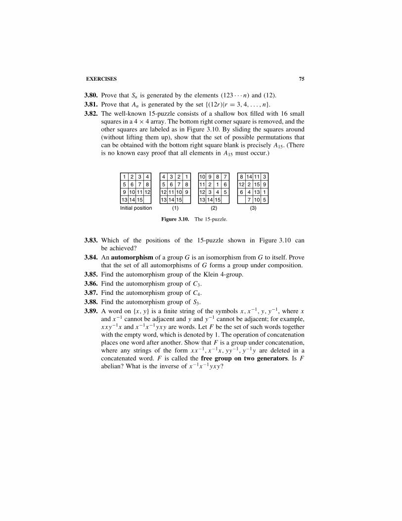
EXERCISES 75
3.80. Prove that Sn is generated by the elements (123 · · · n) and (12).3.81. Prove that An is generated by the set {(12r)|r = 3, 4, . . . , n}.3.82. The well-known 15-puzzle consists of a shallow box filled with 16 small
squares in a 4 × 4 array. The bottom right corner square is removed, and theother squares are labeled as in Figure 3.10. By sliding the squares around(without lifting them up), show that the set of possible permutations thatcan be obtained with the bottom right square blank is precisely A15. (Thereis no known easy proof that all elements in A15 must occur.)
1 2 3 4
5 6 7 8
9 10 11 12
13 14 15
Initial position
4 3 2 1
5 6 7 8
12 11 10 9
13 14 15
(1)
10 9 8 7
11 2 1 6
12 3 4 5
13 14 15
(2)
8 14 11 3
12 2 15 9
6 4 13 1
57 10
(3)
Figure 3.10. The 15-puzzle.
3.83. Which of the positions of the 15-puzzle shown in Figure 3.10 canbe achieved?
3.84. An automorphism of a group G is an isomorphism from G to itself. Provethat the set of all automorphisms of G forms a group under composition.
3.85. Find the automorphism group of the Klein 4-group.3.86. Find the automorphism group of C3.3.87. Find the automorphism group of C4.3.88. Find the automorphism group of S3.3.89. A word on {x, y} is a finite string of the symbols x, x−1, y, y−1, where x
and x−1 cannot be adjacent and y and y−1 cannot be adjacent; for example,xxy−1x and x−1x−1yxy are words. Let F be the set of such words togetherwith the empty word, which is denoted by 1. The operation of concatenationplaces one word after another. Show that F is a group under concatenation,where any strings of the form xx−1, x−1x, yy−1, y−1y are deleted in aconcatenated word. F is called the free group on two generators. Is F
abelian? What is the inverse of x−1x−1yxy?

4QUOTIENT GROUPS
Certain techniques are fundamental to the study of algebra. One such techniqueis the construction of the quotient set of an algebraic object by means of anequivalence relation on the underlying set. For example, if the object is thegroup of integers (Z, +), the congruence relation modulo n on Z will define thequotient group of integers modulo n.
This quotient construction can be applied to numerous algebraic structures,including groups, boolean algebras, and vector spaces.
In this chapter we introduce the concept of an equivalence relation and go onto apply this to groups. We obtain Lagrange’s theorem, which states that the orderof a subgroup divides the order of the group, and we also obtain the morphismtheorem for groups. We study the implications of these two theorems and classifythe groups of low order.
EQUIVALENCE RELATIONS
Relations are one of the basic building blocks of mathematics (as well as of therest of the world). A relation R from a set S to a set T is a subset of S × T .We say that a is related to b under R if the pair (a, b) belongs to the subset,and we write this as aRb. If (a, b) does not belong to the subset, we say that a
is not related to b, and write aR/
b. This definition even covers many relations ineveryday life, such as “is the father of,” “is richer than,” and “goes to the sameschool as” as well as mathematical relations such as “is equal to,” “is a memberof,” and “is similar to.” A relation R from S to T has the property that for anyelements a in S, and b in T , either aRb or aR
/b.
Any function f : S → T gives rise to a relation R from S to T by taking aRbto mean f (a) = b. The subset R of S × T is the graph of the function. However,relations are much more general than functions. One element can be related tomany elements or to no elements at all.
Modern Algebra with Applications, Second Edition, by William J. Gilbert and W. Keith NicholsonISBN 0-471-41451-4 Copyright 2004 John Wiley & Sons, Inc.
76

EQUIVALENCE RELATIONS 77
A relation from a set S to itself is called a relation on S. Any partial orderon a set, such as “�” on the real numbers, or “is a subset of” on a power setP (X), is a relation on that set. “Equals” is a relation on any set S and is definedby the subset {(a, a)|a ∈ S} of S × S. An equivalence relation is a relation thathas the most important properties of the “equals” relation.
A relation E on a set S is called an equivalence relation if the followingconditions hold.
(i) aEa for all a ∈ S. (reflexive condition)(ii) If aEb, then bEa. (symmetric condition)
(iii) If aEb and bEc, then aEc. (transitive condition)
If E is an equivalence relation on S and a ∈ S, then [a] = {x ∈ S|xEa} iscalled the equivalence class containing a. The set of all equivalence classes iscalled the quotient set of S by E and is denoted by S/E. Hence
S/E = {[a]|a ∈ S}.Proposition 4.1. If E is an equivalence relation on a set S, then
(i) If aEb, then [a] = [b].(ii) If aE
/b, then [a] ∩ [b] = Ø.
(iii) S is the disjoint union of all the distinct equivalence classes.
Proof. (i) If aEb, let x be any element of [a]. Then xEa and so xEb bytransitivity. Hence x ∈ [b] and [a] ⊆ [b]. The symmetry of E implies that bEa,and an argument similar to the above shows that [b] ⊆ [a]. This proves that[a] = [b].
(ii) Suppose that aE/
b. If there was an element x ∈ [a] ∩ [b], then xEa, xEb,so aEb by symmetry and transitivity. Hence [a] ∩ [b] = Ø.
(iii) Parts (i) and (ii) show that two equivalence classes are either the same ordisjoint. The reflexivity of E implies that each element a ∈ S is in the equivalenceclass [a]. Hence S is the disjoint union of all the equivalence classes. ��
A collection of nonempty subsets is said to partition a set S if the union ofthe subsets is S and any two subsets are disjoint. The previous proposition showsthat any equivalence relation partitions the set into its equivalence classes. Eachelement of the set belongs to one and only one equivalence class.
It can also be shown that every partition of a set gives rise to an equivalencerelation whose classes are precisely the subsets in the partition.
Example 4.2. Let n be a fixed positive integer and a and b any two integers.We say that a is congruent to b modulo n if n divides a − b. We denotethis by
a ≡ b mod n.

78 4 QUOTIENT GROUPS
Show that this congruence relation modulo n is an equivalence relation on Z. Theset of equivalence classes is called the set of integers modulo n and is denotedby Zn.
Solution. Write “n|m” for “n divides m,” which means that there is someinteger k such that m = nk. Hence a ≡ b mod n if and only if n|(a − b).
(i) For all a ∈ Z, n|(a − a), so a ≡ a mod n and the relation is reflexive.(ii) If a ≡ b mod n, then n|(a − b), so n| − (a − b). Hence n|(b − a) and
b ≡ a mod n.(iii) If a ≡ b mod n and b ≡ c mod n, then n|(a − b) and n|(b − c), so
n|(a − b) + (b − c). Therefore, n|(a − c) and a ≡ c mod n.
Hence congruence modulo n is an equivalence relation on Z. ��
In the congruence relation modulo 3, we have the following equivalence classes:
[0] = {. . . ,−3, 0, 3, 6, 9, . . .}[1] = {. . . ,−2, 1, 4, 7, 10, . . .}[2] = {. . . ,−1, 2, 5, 8, 11, . . .}[3] = {. . . , 0, 3, 6, 9, 12, . . .} = [0]
Any equivalence class must be one of [0], [1], or [2], so Z3 = {[0], [1], [2]}.In general, Zn = {[0], [1], [2], . . . , [n − 1]}, since any integer is congruent
modulo n to its remainder when divided by n.One set of equivalence classes that is introduced in elementary school is the
set of rational numbers. Students soon become used to the fact that 12 and 3
6represent the same rational number. We need to use the concept of equivalenceclass to define a rational number precisely. Define the relation E on Z × Z∗(where Z∗ = Z − {0}) by (a, b) E (c, d) if and only if ad = bc. This is anequivalence relation on Z × Z∗, and the equivalence classes are called rationalnumbers. We denote the equivalence class [(a, b)] by a
b. Therefore, since (1, 2)
E(3, 6), it follows that 12 = 3
6 .Two series-parallel circuits involving the switches A1, A2, . . . , An are said to
be equivalent if they both are open or both are closed for any position of the n
switches. This is an equivalence relation, and the equivalence classes are the 22n
distinct types of circuits controlled by n switches.Any permutation π on a set S induces an equivalence relation, ∼, on S where
a ∼ b if and only if b = πr(a), for some r ∈ Z. The equivalence classes are theorbits of π . In the decomposition of the permutation π into disjoint cycles, theelements in each cycle constitute one orbit.
COSETS AND LAGRANGE’S THEOREM
The congruence relation modulo n on Z can be defined by a ≡ b mod n if andonly if a − b ∈ nZ, where nZ is the subgroup of Z consisting of all multiples

COSETS AND LAGRANGE’S THEOREM 79
of n. We now generalize this notion and define congruence in any group moduloone of its subgroups. We are interested in the equivalence classes, which we callcosets.
Let (G, ·) be a group with subgroup H . For a, b ∈ G, we say that a iscongruent to b modulo H , and write a ≡ b mod H if and only if ab−1 ∈ H .
Proposition 4.3. The relation a ≡ b mod H is an equivalence relation on G. Theequivalence class containing a can be written in the form Ha = {ha|h ∈ H }, andit is called a right coset of H in G. The element a is called a representative ofthe coset Ha.
Proof. (i) For all a ∈ G, aa−1 = e ∈ H ; thus the relation is reflexive.(ii) If a ≡ b mod H , then ab−1 ∈ H ; thus ba−1 = (ab−1)−1 ∈ H . Hence b ≡
a mod H , and the relation is symmetric.(iii) If a ≡ b and b ≡ c mod H , then ab−1 and bc−1 ∈ H . Hence ac1 =
(ab−1)(bc−1) ∈ H and a ≡ c mod H . The relation is transitive. Hence ≡ is anequivalence relation. The equivalence class containing a is
{x ∈ G|x ≡ a mod H } = {x ∈ G|xa−1 = h ∈ H }= {x ∈ G|x = ha, where h ∈ H }= {ha|h ∈ H },
which we denote by Ha. ��
Example 4.4. Find the right cosets of A3 in S3.
Solution. One coset is the subgroup itself A3 = {(1), (123), (132)}. Take anyelement not in the subgroup, say (12). Then another coset is
A3(12) = {(12), (123) Ž (12), (132) Ž (12)} = {(12), (13), (23)}.Since the right cosets form a partition of S3 and the two cosets above contain allthe elements of S3, it follows that these are the only two cosets.
In fact, A3 = A3(123) = A3(132) and A3(12) = A3(13) = A3(23). ��
Example 4.5. Find the right cosets of H = {e, g4, g8} in C12 = {e, g, g2, . . . , g11}.Solution. H itself is one coset. Another is Hg = {g, g5, g9}. These two cosets
have not exhausted all the elements of C12, so pick an element, say g2, whichis not in H or Hg. A third coset is Hg2 = {g2, g6, g10} and a fourth is Hg3 ={g3, g7, g11}.
Since C12 = H ∪ Hg ∪ Hg2 ∪ Hg3, these are all the cosets. ��
As the examples above suggest, every coset contains the same number ofelements. We use this result to prove the famous theorem of Joseph Lagrange(1736–1813).

80 4 QUOTIENT GROUPS
Lemma 4.6. There is a bijection between any two right cosets of H in G.
Proof. Let Ha be a right coset of H in G. We produce a bijection betweenHa and H , from which it follows that there is a bijection between any tworight cosets.
Define ψ : H → Ha by ψ(h) = ha. Then ψ is clearly surjective. Now supposethat ψ(h1) = ψ(h2), so that h1a = h2a. Multiplying each side by a−1 on theright, we obtain h1 = h2. Hence ψ is a bijection. �
Theorem 4.7. Lagrange’s Theorem. If G is a finite group and H is a subgroupof G, then |H | divides |G|.
Proof. The right cosets of H in G form a partition of G, so G can be writtenas a disjoint union
G = Ha1 ∪ Ha2 ∪ · · · ∪ Hak for a finite set of elements a1, a2, . . . , ak ∈ G.
By Lemma 4.6, the number of elements in each coset is |H |. Hence, countingall the elements in the disjoint union above, we see that |G| = k|H |. Therefore,|H | divides |G|. �
If H is a subgroup of G, the number of distinct right cosets of H in G iscalled the index of H in G and is written |G : H |. The following is a directconsequence of the proof of Lagrange’s theorem.
Corollary 4.8. If G is a finite group with subgroup H , then
|G : H | = |G|/|H |.
Corollary 4.9. If a is an element of a finite group G, then the order of a dividesthe order of G.
Proof. Let H = {ar |r ∈ Z} be the cyclic subgroup generated by a. By Propo-sition 3.13, the order of the subgroup H is the same as the order of the elementa. Hence, by Lagrange’s theorem, the order of a divides the order of G. ��
Corollary 4.10. If a is an element of the finite group G, then a|G| = e.
Proof. If m is the order of a, then |G| = mk for some integer k. Hence a|G| =amk = (am)k = ek = e. ��
Corollary 4.11. If G is a group of prime order, then G is cyclic.
Proof. Let |G| = p, a prime number. By Corollary 4.9, every element hasorder 1 or p. But the only element of order 1 is the identity. Therefore, all the

COSETS AND LAGRANGE’S THEOREM 81
other elements have order p, and there is at least one because |G| � 2. Henceby Theorem 3.14, G is a cyclic group. ��
The converse of Lagrange’s theorem is false, as the following example shows.That is, if k is a divisor of the order of G, it does not necessarily follow that G
has a subgroup of order k.
Example 4.12. A4 is a group of order 12 having no subgroup of order 6.
Solution. A4 contains one identity element, eight 3-cycles of the form (abc),and three pairs of transpositions of the form (ab) Ž (cd), where a, b, c, andd are distinct elements of {1, 2, 3, 4}. If a subgroup contains a 3-cycle (abc),it must also contain its inverse (acb). If a subgroup of order 6 exists, it mustcontain the identity and a product of two transpositions, because the odd numberof nonidentity elements cannot be made up of 3-cycles and their inverses. Asubgroup of order 6 must also contain at least two 3-cycles because A4 onlycontains four elements that are not 3-cycles.
Without loss of generality, suppose that a subgroup of order 6 contains theelements (abc) and (ab) Ž (cd). Then it must also contain the elements (abc)−1 =(acb), (abc) Ž (ab) Ž (cd) = (acd), (ab) Ž (cd) Ž (abc) = (bdc), and (acd)−1 =(adc), which, together with the identity, gives more than six elements. Hence A4
contains no subgroup of order 6. ��
The next proposition strengthens Lagrange’s theorem in the case of finitecyclic groups. The following lemma, of interest in its own right, will be needed.
Lemma 4.13. Let g be an element of order n in a group, and let m � 1.
(i) If gcd(n, m) = d , then gm has order n/d.(ii) In particular, if m divides n, then gm has order n/m.
Proof. (i). We have (gm)n/d = (gn)m/d = em/d = e. If (gm)k = e, we must
show thatn
ddivides k. We have gmk = e, so n divides mk by Proposition 3.11.
Hencen
ddivides
m
dk. But
n
dand
m
dare relatively prime by Theorem 11,
Appendix 2, son
ddivides k (by the same theorem).
(ii). If m divides n, then gcd(n, m) = m, so (i) implies (ii). ��
Proposition 4.14. If G is a cyclic group of order n, and if k divides n, thenG has exactly one subgroup H of order k. In fact, if g generates G, then H isgenerated by gn/k.
Proof. Let H denote the subgroup generated by gn/k. Then |H | = k because
gn/k has order k by Lemma 4.13(
with m = n
k
). Now let K be any subgroup of
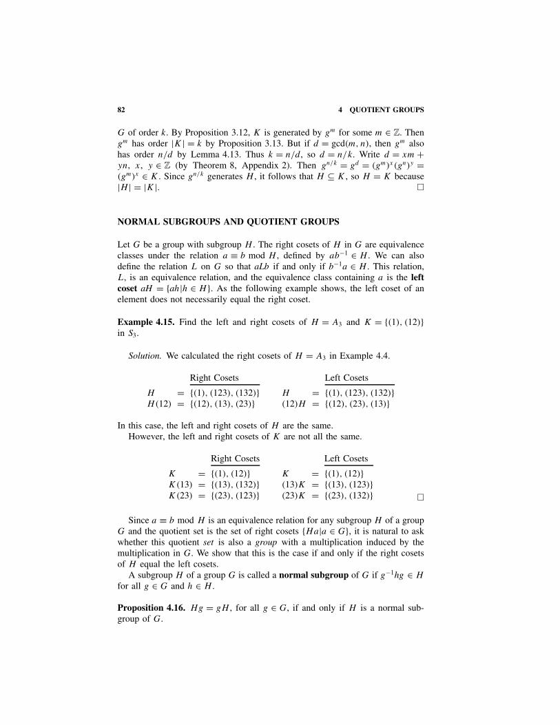
82 4 QUOTIENT GROUPS
G of order k. By Proposition 3.12, K is generated by gm for some m ∈ Z. Thengm has order |K| = k by Proposition 3.13. But if d = gcd(m, n), then gm alsohas order n/d by Lemma 4.13. Thus k = n/d , so d = n/k. Write d = xm +yn, x, y ∈ Z (by Theorem 8, Appendix 2). Then gn/k = gd = (gm)x(gn)y =(gm)x ∈ K . Since gn/k generates H , it follows that H ⊆ K , so H = K because|H | = |K|. �
NORMAL SUBGROUPS AND QUOTIENT GROUPS
Let G be a group with subgroup H . The right cosets of H in G are equivalenceclasses under the relation a ≡ b mod H , defined by ab−1 ∈ H . We can alsodefine the relation L on G so that aLb if and only if b−1a ∈ H . This relation,L, is an equivalence relation, and the equivalence class containing a is the leftcoset aH = {ah|h ∈ H }. As the following example shows, the left coset of anelement does not necessarily equal the right coset.
Example 4.15. Find the left and right cosets of H = A3 and K = {(1), (12)}in S3.
Solution. We calculated the right cosets of H = A3 in Example 4.4.
Right Cosets Left Cosets
H = {(1), (123), (132)} H = {(1), (123), (132)}H(12) = {(12), (13), (23)} (12)H = {(12), (23), (13)}
In this case, the left and right cosets of H are the same.However, the left and right cosets of K are not all the same.
Right Cosets Left Cosets
K = {(1), (12)} K = {(1), (12)}K(13) = {(13), (132)} (13)K = {(13), (123)}K(23) = {(23), (123)} (23)K = {(23), (132)} �
Since a ≡ b mod H is an equivalence relation for any subgroup H of a groupG and the quotient set is the set of right cosets {Ha|a ∈ G}, it is natural to askwhether this quotient set is also a group with a multiplication induced by themultiplication in G. We show that this is the case if and only if the right cosetsof H equal the left cosets.
A subgroup H of a group G is called a normal subgroup of G if g−1hg ∈ H
for all g ∈ G and h ∈ H .
Proposition 4.16. Hg = gH , for all g ∈ G, if and only if H is a normal sub-group of G.

NORMAL SUBGROUPS AND QUOTIENT GROUPS 83
Proof. Suppose that Hg = gH . Then, for any element h ∈ H, hg ∈ Hg =gH . Hence hg = gh1 for some h1 ∈ H and g−1hg = g−1gh1 = h1 ∈ H . There-fore, H is a normal subgroup.
Conversely, if H is normal, let hg ∈ Hg and g−1hg = h1 ∈ H . Then hg =gh1 ∈ gH and Hg ⊆ gH . Also, ghg−1 = (g−1)−1hg−1 = h2 ∈ H , since H isnormal, so gh = h2g ∈ Hg. Hence, gH ⊆ Hg, and so Hg = gH . �
Therefore, A3 is a normal subgroup of S3 by Example 4.13, whereas {(1), (12)}is not.
Proposition 4.17. Any subgroup of an abelian group is normal.
Proof. If H is a subgroup of an abelian group, G, then g−1hg = hg−1g =h ∈ H for all g ∈ G, h ∈ H . Hence H is normal. ��
If N is a normal subgroup of a group G, the left cosets of N in G are thesame as the right cosets of N in G, so there will be no ambiguity in just talkingabout the cosets of N in G.
Theorem 4.18. If N is a normal subgroup of (G, ·), the set of cosets G/N ={Ng|g ∈ G} forms a group (G/N , ·), where the operation is defined by(Ng1) · (Ng2) = N(g1 · g2). This group is called the quotient group or factorgroup of G by N .
Proof. The operation of multiplying two cosets, Ng1 and Ng2, is defined interms of particular elements, g1 and g2, of the cosets. For this operation to makesense, we have to verify that, if we choose different elements, h1 and h2, inthe same cosets, the product coset N(h1 · h2) is the same as N(g1 · g2). In otherwords, we have to show that multiplication of cosets is well defined.
Since h1 is in the same coset as g1, we have h1 ≡ g1 mod N . Similarly,h2 ≡ g2 mod N . We show that Nh1h2 = Ng1g2. We have h1g
−11 = n1 ∈
N and h2g−12 = n2 ∈ N , so h1h2(g1g2)
−1 = h1h2g−12 g−1
1 = n1g1n2g2g−12 g−1
1 =n1g1n2g
−11 . Now N is a normal subgroup, so g1n2g
−11 ∈ N and n1g1n2g
−11 ∈ N .
Hence h1h2 ≡ g1g2 mod N and Nh1h2 = Ng1g2. Therefore, the operation iswell defined.
The operation is associative because (Ng1 · Ng2) · Ng3 = N(g1g2) · Ng3 =N(g1g2)g3 and also Ng1 · (Ng2 · Ng3) = Ng1 · N(g2g3) = Ng1(g2g3) =N(g1g2)g3.
Since Ng · Ne = Nge = Ng and Ne · Ng = Ng, the identity is Ne = N . Theinverse of Ng is Ng−1 because Ng · Ng−1 = N(g · g−1) = Ne = N and alsoNg−1 · Ng = N .
Hence (G/N, ·) is a group. ��
The order of G/N is the number of cosets of N in G. Hence
|G/N | = |G : N | = |G|/|N |.

84 4 QUOTIENT GROUPS
TABLE 4.1. QuotientGroup S3/A3
Ž H H (12)
H H H (12)H (12) H (12) H
We have seen in Example 4.15 that A3 is a normal subgroup of S3; therefore,S3/A3 is a quotient group. If H = A3, the elements of this group are the cosetsH and H (12), and its multiplication table is given in Table 4.1.
Example 4.19. (Zn, +) is the quotient group of (Z, +) by the subgroup nZ ={nz|z ∈ Z}.
Solution. Since (Z,+) is abelian, every subgroup is normal. The set nZ canbe verified to be a subgroup, and the relationship a ≡ b mod nZ is equivalentto a − b ∈ nZ and to n|a − b. Hence a ≡ b mod nZ is the same relation asa ≡ b mod n. Therefore, Zn is the quotient group Z/nZ, where the operation oncongruence classes is defined by [a] + [b] = [a + b]. �
(Zn, +) is a cyclic group with 1 as a generator, and therefore, by Theorem 3.25,is isomorphic to Cn. The group (Z5, +) is shown in Table 4.2.
When there is no confusion, we write the elements of Zn as 0, 1, 2, 3, . . . ,
n − 1 instead of [0], [1], [2], [3], . . . , [n − 1].
Proposition 4.20. If H is a subgroup of index 2 in G, so that |G : H | = 2, thenH is a normal subgroup of G, and G/H is cyclic group of order 2.
Proof. Since |G : H | = 2, there are only two right cosets of H in G. Onemust be H and the other can be written as Hg, where g is any element of G thatis not in H . To show that H is a normal subgroup of G, we need to show thatg−1hg ∈ H for all g ∈ G and h ∈ H . If g is an element of H , it is clear thatg−1hg ∈ H for all h ∈ H . If g is not an element of H , suppose that g−1hg /∈ H .In this case, g−1hg must be an element of the other right coset Hg, and wecan write g−1hg = h1g, for some h1 ∈ H . It follows that g = hh−1
1 ∈ H , whichcontradicts the fact that g /∈ H . Hence g−1hg ∈ H for all g ∈ G and h ∈ H ; inother words, H is normal in G. ��
TABLE 4.2. Group (Z5, +)
+ [0] [1] [2] [3] [4][0] [0] [1] [2] [3] [4][1] [1] [2] [3] [4] [0][2] [2] [3] [4] [0] [1][3] [3] [4] [0] [1] [2][4] [4] [0] [1] [2] [3]

NORMAL SUBGROUPS AND QUOTIENT GROUPS 85
Theorem 4.21. If G is a finite abelian group and the prime p divides the orderof G, then G contains an element of order p and hence a subgroup of order p.
Proof. We prove this result by induction on the order of G. For a particularprime p, suppose that all abelian groups of order less than k, whose order isdivisible by p, contain an element of order p. The result is vacuously true forgroups of order 1. Now suppose that G is a group of order k. If p divides k,choose any nonidentity element g ∈ G. Let t be the order of the element g.
Case 1. If p divides t , say t = pr , then gr is an element of order p. This followsbecause gr is not the identity, but (gr)p = gt = e, and p is a prime.
Case 2. On the other hand, if p does not divide t , let K be the subgroup generatedby g. Since G is abelian, K is normal, and the quotient group G/K has order|G|/t , which is divisible by p. Therefore, by the induction hypothesis, G/K hasan element of order p, say Kh. If u is the order of h in G, then hu = e and(Kh)u = Khu = K . Since Kh has order p in G/K , u is a multiple of p, and weare back to case 1.
The result now follows from the principle of mathematical induction. �
This result is a partial converse to Lagrange’s theorem. It is a special case ofsome important results, in more advanced group theory, known as the Sylow the-orems. These theorems give information on the subgroups of prime power order,and they can be found in books such as Herstein [9], Hall [30], or Nicholson [11].
Example 4.22. Show that A5 has no proper normal subgroups.
Solution. It follows from Corollary 3.34 that A5 contains three types of non-identity elements: 3-cycles, 5-cycles, and pairs of disjoint transpositions. Supposethat N is a normal subgroup of A5 that contains more than one element.
Case 1. Suppose that N contains the 3-cycle (abc). From the definition of nor-mal subgroup, g−1 Ž (abc) Ž g ∈ N for all g ∈ A5. If we take g = (ab) Ž (cd),we obtain
(ab) Ž (cd) Ž (abc) Ž (ab) Ž (cd) = (adb) ∈ N
and also (adb)−1 = (abd) ∈ N . In a similar way, we can show that N containsevery 3-cycle. Therefore, by Proposition 3.37, N must be the entire alternat-ing group.
Case 2. Suppose that N contains the 5-cycle (abcde). Then
and (abc)−1 Ž (abcde) Ž (abc) = (acb) Ž (abcde) Ž (abc) = (abdec) ∈ N
(abcde) Ž (abdec)−1 = (abcde) Ž (acedb) = (adc) ∈ N.
We are now back to case 1, and hence N = A5.

86 4 QUOTIENT GROUPS
Case 3. Suppose that N contains the pair of disjoint transpositions (ab) Ž (cd).Then, if e is the element of {1, 2, 3, 4, 5} not appearing in these transpositions,we have
(abe)−1 Ž (ab) Ž (cd) Ž (abe) = (aeb) Ž (ab) Ž (cd) Ž (abe) = (ae) Ž (cd) ∈ N.
Also, (ab) Ž (cd) Ž (ae) Ž (cd) = (aeb) ∈ N , and again we are back to case 1.
We have shown that any normal subgroup of A5 containing more than oneelement must be A5 itself. �
A group without any proper normal subgroups is called a simple group. Theterm simple must be understood in the technical sense that it cannot be brokendown, because it cannot have any nontrivial quotient groups. This is analogous toa prime number, which has no nontrivial quotients. Apart from the cyclic groupsof prime order, which have no proper subgroups of any kind, simple groups arecomparatively rare.
The group A5 is of great interest to mathematicians because it is used in Galoistheory to show that there is an equation of the fifth degree that cannot be solvedby any algebraic formula.
It can be shown that every alternating group An, n � 5, is simple. The cyclicgroups Cp, p a prime, are another infinite series of simple groups (the abelianones), and other series have been known for decades. But it was not until 1981that the finite simple groups were completely classified. This was the culmina-tion of more than 30 years of effort by hundreds of mathematicians, yieldingthousands of pages of published work, and was one of the great achievements oftwentieth-century mathematics. One spectacular landmark came in 1963, whenJ. G. Thompson and W. Feit verified a long-standing conjecture of W. Burnside(1852–1927) that every finite, non-abelian, simple group has even order (theproof is more than 250 pages long!). The main difficulty in the classification wasthe existence of sporadic finite simple groups, not belonging to any of the knownfamilies. The largest of these, known as the monster, has order approximately2 × 1053. The complete classification encompasses several infinite families andexactly 26 sporadic groups.
MORPHISM THEOREM
The morphism theorem is a basic result of group theory that describes the rela-tionship between morphisms, normal subgroups, and quotient groups. There is ananalogous result for most algebraic systems, including rings and vector spaces.
If f : G → H is a group morphism, the kernel of f , denoted by Kerf , isdefined to be the set of elements of G that are mapped by f to the identity ofH . That is, Kerf = {g ∈ G|f (g) = eH }.Proposition 4.23. Let f : G → H be a group morphism. Then:
(i) Kerf is a normal subgroup of G.(ii) f is injective if and only if Kerf = {eG}.
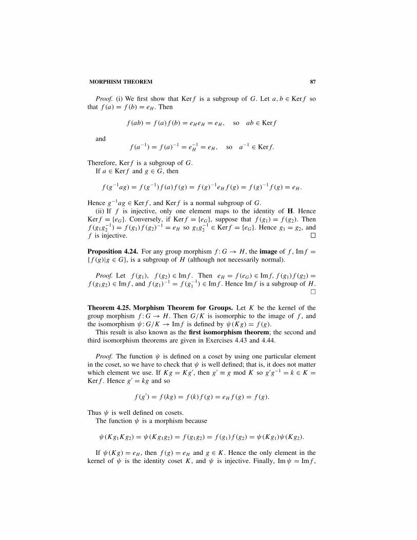
MORPHISM THEOREM 87
Proof. (i) We first show that Kerf is a subgroup of G. Let a, b ∈ Kerf sothat f (a) = f (b) = eH . Then
f (ab) = f (a)f (b) = eHeH = eH , so ab ∈ Kerf
andf (a−1) = f (a)−1 = e−1
H = eH , so a−1 ∈ Kerf.
Therefore, Kerf is a subgroup of G.If a ∈ Kerf and g ∈ G, then
f (g−1ag) = f (g−1)f (a)f (g) = f (g)−1eHf (g) = f (g)−1f (g) = eH .
Hence g−1ag ∈ Kerf , and Kerf is a normal subgroup of G.(ii) If f is injective, only one element maps to the identity of H. Hence
Kerf = {eG}. Conversely, if Kerf = {eG}, suppose that f (g1) = f (g2). Thenf (g1g
−12 ) = f (g1)f (g2)
−1 = eH so g1g−12 ∈ Kerf = {eG}. Hence g1 = g2, and
f is injective. ��
Proposition 4.24. For any group morphism f : G → H , the image of f , Imf ={f (g)|g ∈ G}, is a subgroup of H (although not necessarily normal).
Proof. Let f (g1), f (g2) ∈ Imf . Then eH = f (eG) ∈ Imf, f (g1)f (g2) =f (g1g2) ∈ Imf , and f (g1)
−1 = f (g−11 ) ∈ Imf . Hence Imf is a subgroup of H .
�
Theorem 4.25. Morphism Theorem for Groups. Let K be the kernel of thegroup morphism f : G → H . Then G/K is isomorphic to the image of f , andthe isomorphism ψ : G/K → Imf is defined by ψ(Kg) = f (g).
This result is also known as the first isomorphism theorem; the second andthird isomorphism theorems are given in Exercises 4.43 and 4.44.
Proof. The function ψ is defined on a coset by using one particular elementin the coset, so we have to check that ψ is well defined; that is, it does not matterwhich element we use. If Kg = Kg′, then g′ ≡ g mod K so g′g−1 = k ∈ K =Kerf . Hence g′ = kg and so
f (g′) = f (kg) = f (k)f (g) = eHf (g) = f (g).
Thus ψ is well defined on cosets.The function ψ is a morphism because
ψ(Kg1Kg2) = ψ(Kg1g2) = f (g1g2) = f (g1)f (g2) = ψ(Kg1)ψ(Kg2).
If ψ(Kg) = eH , then f (g) = eH and g ∈ K . Hence the only element in thekernel of ψ is the identity coset K , and ψ is injective. Finally, Im ψ = Imf ,

88 4 QUOTIENT GROUPS
by the definition of ψ . Therefore, ψ is the required isomorphism between G/K
and Imf . �
Conversely, note that if K is any normal subgroup of G, the map g → Kg isa morphism from G to G/K , whose kernel is precisely K .
By taking f to be the identity morphism from G to itself, the morphismtheorem implies that G/{e} ∼= G.
The function f : Z → Zn, defined by f (x) = [x], has nZ as its kernel, andtherefore the morphism theorem yields the fact that Z/nZ ∼= Zn.
If a and b are generators of the cyclic groups C12 = 〈a〉 and C6 = 〈b〉, respec-tively, consider the function f : C12 → C6 given by f (ar) = b2r . This is welldefined. In fact, if ar = ar1 , then 12 divides r − r1 by Proposition 3.11, so cer-tainly b2r = b2r1 . It is easily verified that f is morphism, and the kernel isK = {e, a3, a6, a9} because if ar is in K , then b2r = 0, so 6 divides 2r , whence3 divides r . Thus C12/K ∼= C6, and this isomorphism is obtained by mappingthe coset Kar to b2r .
The alternating group An is of index 2 in the symmetric group Sn (by The-orem 3.36) and so is a normal subgroup by Proposition 4.20. It is instructiveto obtain this same conclusion from the morphism theorem. If σ is a per-mutation in Sn, recall that σ is called even or odd according as σD = D orσD = −D, where D is the discriminant in n variables (see the discussion lead-ing to Theorem 3.33). Consider the multiplicative group {1, −1}, and define a
function f : Sn → {1,−1} by f (σ) ={
1 if σD = D
−1 if σD = −D. Then f is a surjec-
tive morphism (verify) and the kernel is the group An of even permutations. Since|Sn| = n!, the morphism theorem and Corollary 4.8 give the following result (andreprove Theorem 3.36).
Proposition 4.26. An is a normal subgroup of Sn, Sn/An∼= C2, and |An| = 1
2n!.
Example 4.27. Show that the quotient group R/Z, of real numbers modulo 1 isisomorphic to the circle group W = {eiθ ∈ C|θ ∈ R}.
Solution. The set W consists of points on the circle of complex numbersof unit modulus, and forms a group under multiplication. Define the functionf : R → W by f (x) = e2πix . This is a morphism from (R, +) to (W, ·) because
f (x + y) = e2πi(x+y) = e2πix · e2πiy = f (x) · f (y).
This function can be visualized in Figure 4.1 as wrapping the real line aroundand around the circle.
The morphism f is clearly surjective, and its kernel is {x ∈ R|e2πix = 1} = Z.Therefore, the morphism theorem implies that R/Z ∼= W . The quotient space R/Z
is the set of equivalence classes of R under the relation defined by x ≡ y mod Z
if and only if the real numbers x and y differ by an integer. This quotient spaceis called the group of real numbers modulo 1. �

MORPHISM THEOREM 89
−2 −1 0 1 2 3
−1
−i
i
f
W
1
Figure 4.1. Morphism f : R → W .
Proposition 4.28. If G and H are finite groups whose orders are relatively prime,there is only one morphism from G to H , the trivial one.
Proof. Let K be the kernel of a morphism f from G to H . Then G/K ∼= Imf ,a subgroup of H . Now |G/K| = |G|/|K|, which is a divisor of |G|. But byLagrange’s theorem, |Imf | is a divisor of |H |. Since |G| and |H | are relativelyprime, we must have |G/K| = |Imf | = 1. Therefore K = G, so f : G → H isthe trivial morphism defined by f (g) = eH for all g ∈ G. �
Example 4.29. Find all the subgroups and quotient groups of D4, the symmetrygroup of a square, and draw the poset diagram of its subgroups.
Solution. Any symmetry of the square induces a permutation of its vertices.Thus, as in Example 3.30, this defines a group morphism f : D4 → S4. How-ever, unlike the case of the symmetries of an equilateral triangle, this is not anisomorphism because |D4| = 8, whereas |S4| = 24. The kernel of f consists ofsymmetries fixing the vertices and so consists of the identity only. Therefore, bythe morphism theorem, D4 is isomorphic to the image of f in S4. We equatean element of D4 with its image in S4. All the elements of D4 are shown inFigure 4.2. The corner by the vertex 1 is blocked in, and the reverse side of thesquare is shaded to illustrate the effect of the symmetries. The order of eachsymmetry is given in Table 4.3.
21
34
21
34
21
34
21
34
(1) = e (1234) = g (13)°(24) = g2 (1432) = g3
21
34
21
34
21
34
21
34
(24) = h (12) ° (34) = gh (13) = g2h (14) ° (23) = g3h
Figure 4.2. Symmetries of the square.

90 4 QUOTIENT GROUPS
TABLE 4.3. Orders of the Symmetries of a Square
Elements of D4 e g g2 g3 h gh g2h g3h
Order of Element 1 4 2 4 2 2 2 2
e, g2h
e
e, h e, g3he, gh
D4
C4
e, g2 = L
e, g2,h, g2hK1 = e, g2, gh, g3h = K2
Figure 4.3. Poset diagram of subgroups of D4.
The cyclic subgroups generated by the elements are {e}, C4 = {e, g, g2, g3},{e, g2}, {e, h}, {e, gh}, {e, g2h}, and {e, g3h}.
By Lagrange’s theorem, any proper subgroup must have order 2 or 4. Sinceany group of order 2 is cyclic, the only proper subgroups that are not cyclic areof order 4 and contain elements of order 1 and 2. There are two such subgroups,K1 = {e, g2, h, g2h} and K2 = {e, g2, gh, g3h}. All the subgroups are illustratedin Figure 4.3.
To find all the quotient groups, we must determine which subgroups arenormal.
The trivial group {e} and the whole group D4 are normal subgroups. SinceC4, K1, and K2 have index 2 in D4, they are normal by Proposition 4.20, andtheir quotient groups are cyclic of order 2.
Subgroup H Left Coset gH Right Coset Hg
{e, h} {g, gh} {g, hg} = {g, g3h}{e, g2h} {g, g3h} {g, g2hg} = {g, gh}{e, gh} {g, g2h} {g, ghg} = {g, h}{e, g3h} {g, h} {g, g3hg} = {g, g2h}
For each of the subgroups above, the left and right cosets containing g aredifferent; therefore, none of the subgroups are normal.
Left Cosets of L Right Cosets of L
L = {e, g2} L = {e, g2}gL = {g, g3} Lg = {g, g3}hL = {h, hg2} = {h, g2h} Lh = {h, g2h}
ghL = {gh, ghg2} = {gh, g3h} Lgh = {gh, g3h}The table above shows that L = {e, g2} is a normal subgroup. The multipli-
cation table for D4/L given in Table 4.4 shows that it is isomorphic to the Klein4-group. �

DIRECT PRODUCTS 91
TABLE 4.4. Group D4/L
· L Lh Lg Lgh
L L Lh Lg LghLh Lh L Lgh LgLg Lg Lgh L LhLgh Lgh Lg Lh L
DIRECT PRODUCTS
Given two sets, S and T , we can form their Cartesian product, S × T = {(s, t)|s ∈S, t ∈ T }, whose elements are ordered pairs. For example, the product of the realline, R, with itself is the plane, R × R = R2. We now show how to define theproduct of any two groups; the underlying set of the product is the Cartesianproduct of the underlying sets of the original groups.
Proposition 4.30. If (G, Ž ) and (H , �) are two groups, then (G × H, ·) is agroup under the operation · defined by
(g1, h1) · (g2, h2) = (g1 Ž g2, h1 � h2).
The group (G × H, ·) is called the direct product of the groups (G, Ž ) and (H , �).
Proof. All the group axioms follow from the axioms for (G, Ž ) and (H , �).The identity of G × H is (eG, eH ), and the inverse of (g, h) is (g−1, h−1). �
This construction can be iterated any finite number of times to obtain thedirect product of n groups.
Sometimes the direct product of two groups G and H is called the directsum and is denoted by G ⊕ H . (The direct sum of a finite number of groups isthe same as the direct product. It is possible to define a direct sum and directproduct of an infinite number of groups; these are different. An element of thedirect product is obtained by taking one element from each group, while anelement of the direct sum is obtained by taking one element from each group,but with only a finite number different from the identity.)
Example 4.31. Write down the table for the direct product of C2 with itself.
Solution. Let C2 = {e, g}, so that C2 × C2 = {(e, e), (e, g), (g, e), (g, g)}. Itstable is given in Table 4.5. We see that this group C2 × C2 is isomorphic to theKlein 4-group of symmetries of a rectangle. �
Theorem 4.32. If gcd(m, n) = 1, then Cmn∼= Cm × Cn.
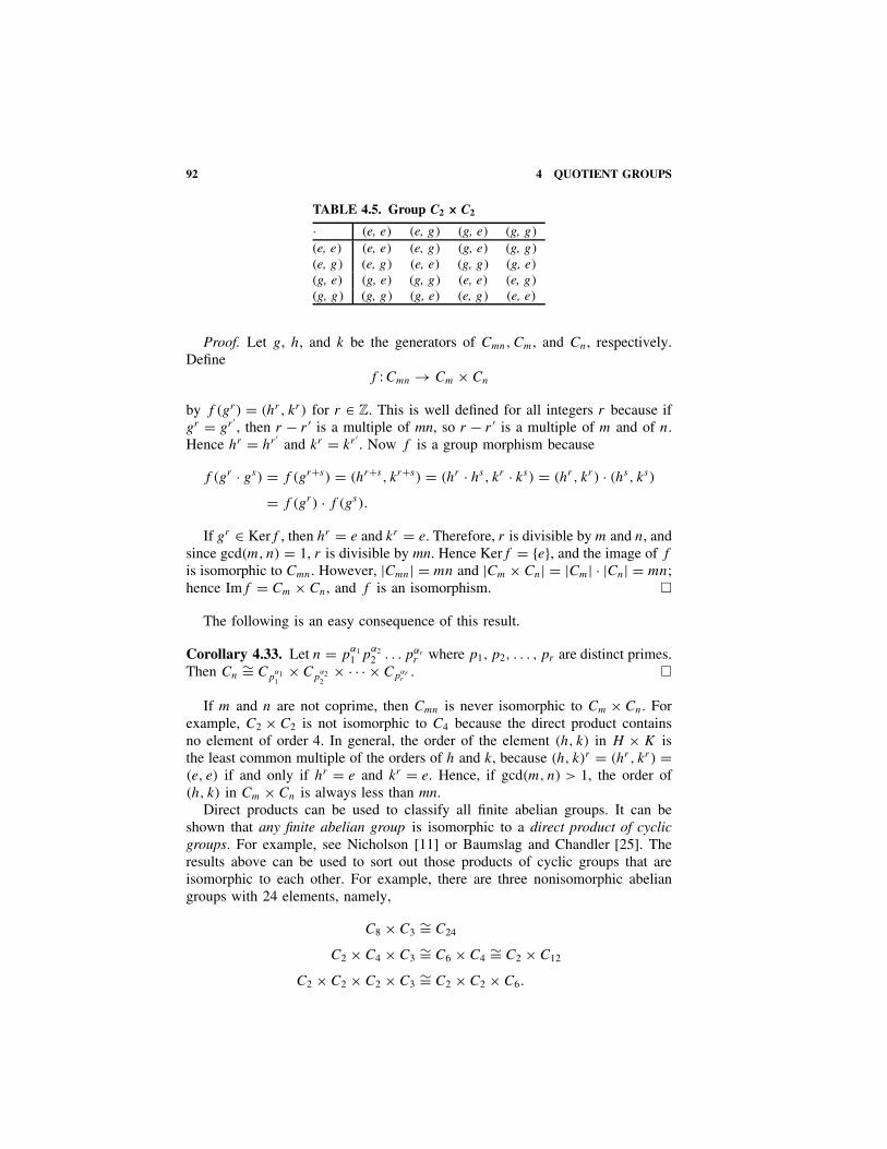
92 4 QUOTIENT GROUPS
TABLE 4.5. Group C2 × C2
· (e, e) (e, g) (g, e) (g, g)(e, e) (e, e) (e, g) (g, e) (g, g)(e, g) (e, g) (e, e) (g, g) (g, e)(g, e) (g, e) (g, g) (e, e) (e, g)(g, g) (g, g) (g, e) (e, g) (e, e)
Proof. Let g, h, and k be the generators of Cmn, Cm, and Cn, respectively.Define
f : Cmn → Cm × Cn
by f (gr) = (hr , kr) for r ∈ Z. This is well defined for all integers r because ifgr = gr ′
, then r − r ′ is a multiple of mn, so r − r ′ is a multiple of m and of n.Hence hr = hr ′
and kr = kr ′. Now f is a group morphism because
f (gr · gs) = f (gr+s) = (hr+s , kr+s) = (hr · hs, kr · ks) = (hr, kr) · (hs, ks)
= f (gr) · f (gs).
If gr ∈ Kerf , then hr = e and kr = e. Therefore, r is divisible by m and n, andsince gcd(m, n) = 1, r is divisible by mn. Hence Kerf = {e}, and the image of f
is isomorphic to Cmn. However, |Cmn| = mn and |Cm × Cn| = |Cm| · |Cn| = mn;hence Imf = Cm × Cn, and f is an isomorphism. �
The following is an easy consequence of this result.
Corollary 4.33. Let n = pα11 p
α22 . . . pαr
r where p1, p2, . . . , pr are distinct primes.Then Cn
∼= Cpα11
× Cpα22
× · · · × Cpαrr
. �
If m and n are not coprime, then Cmn is never isomorphic to Cm × Cn. Forexample, C2 × C2 is not isomorphic to C4 because the direct product containsno element of order 4. In general, the order of the element (h, k) in H × K isthe least common multiple of the orders of h and k, because (h, k)r = (hr, kr) =(e, e) if and only if hr = e and kr = e. Hence, if gcd(m, n) > 1, the order of(h, k) in Cm × Cn is always less than mn.
Direct products can be used to classify all finite abelian groups. It can beshown that any finite abelian group is isomorphic to a direct product of cyclicgroups. For example, see Nicholson [11] or Baumslag and Chandler [25]. Theresults above can be used to sort out those products of cyclic groups that areisomorphic to each other. For example, there are three nonisomorphic abeliangroups with 24 elements, namely,
C8 × C3∼= C24
C2 × C4 × C3∼= C6 × C4
∼= C2 × C12
C2 × C2 × C2 × C3∼= C2 × C2 × C6.

DIRECT PRODUCTS 93
Theorem 4.34. If (G, ·) is a finite group for which every element g ∈ G satisfiesg2 = e, then |G| = 2n for some n � 0, and G is isomorphic to the n-fold directproduct Cn
2 = C2 × C2 × · · · × C2.
Proof. Every element in G has order 1 or 2, and the identity is the onlyelement of order 1. Therefore, every element of G is its own inverse. The groupG is abelian because for any g, h ∈ G, gh = (gh)−1 = h−1g−1 = hg.
Choose the elements a1, a2, . . . , an ∈ G so that ai �= e and ai cannot be writtenas a product of powers of a1, . . . , ai−1. Furthermore, choose n maximal, so thatevery element can be written in terms of the elements ai . If C2 is generated byg, we show that the function
f : Cn2 → G, defined by f (gr1 , gr2, . . . , grn) = a
r11 a
r22 . . . arn
n
is an isomorphism. It is well defined for all integers ri , because if gri = gqi , thena
ri
i = aqi
i . Now
f ((gr1, . . . , grn) · (gs1 , . . . , gsn)) = f (gr1+s1, . . . , grn+sn ) = ar1+s11 . . . arn+sn
n
= ar11 . . . arn
n .as11 . . . asn
n because G is abelian
= f (gr1, . . . , grn) · f (gs1, . . . , gsn).
Hence f is a group morphism.Let (gr1 , . . . , grn) ∈ Kerf . Suppose that ri is the last odd exponent, so that
ri+1, ri+2, . . . , rn are all even. Then ar1...
1 ari−1
i−1ai = e and
ai = a−1i = a
r1...
1 ari−1
i−1,
which is a contradiction. Therefore, all the exponents are even, and f is injective.The choice of the elements ai guarantees that f is surjective. Hence f is therequired isomorphism. �
Example 4.35. Describe all the group morphisms from C10 to C2 × C5. Whichof these are isomorphisms? �
Solution. Since C10 is a cyclic group, generated by g, for example, a morphismfrom C10 is determined by the image of g. Let h and k be generators of C2 and C5,respectively, and consider the function fr,s : C10 → C2 × C5 which maps g to theelement (hr, ks) ∈ C2 × C5. Then, if fr,s is a morphism, fr,s(g
n) = (hrn, ksn) for0 � n�9. However, this would also be true for all integers n, because if gn = gm,then 10|n − m. Hence 2|n − m and 5|n − m and hrn = hrm and ksn = ksm.
We now verify that fr,s is a morphism for any r and s. We have
fr,s(gagb) = fr,s(g
a+b) = (h(a+b)r , k(a+b)s) = (har , kas)(hbr , kbs)
= fr,s(ga)fr,s (g
b).

94 4 QUOTIENT GROUPS
Therefore, there are ten morphisms, fr,s , from C10 to C2 × C5 corresponding tothe ten elements (hr, ks) of C2 × C5.
Now
Kerfr,s = {gn|(hrn, ksn) = (e, e)} = {gn|rn ≡ 0 mod 2 and sn ≡ 0 mod 5}.
Hence Kerfr,s = {e} if (r, s) = (1, 1), (1, 2), (1, 3), or (1, 4), while Kerf0,0 =C10, Kerf1,0 = {e, g2, g4, g6, g8}, and Kerf0,s = {e, g5}, if s = 1, 2, 3, or 4. IfKerfr,s contains more than one element, fr,s is not an injection and cannot be anisomorphism. By the morphism theorem,
|C10|/|Kerfr,s | = |Imfr,s |,
and if Kerfr,s = {e}, then | Im fr,s | = 10, so fr,s is surjective also. Therefore, theisomorphisms are f1,1, f1,2, f1,3, and f1,4. ��
GROUPS OF LOW ORDER
We find all possible isomorphism classes of groups with eight or fewer elements.
Lemma 4.36. Suppose that a and b are elements of coprime orders r and s,respectively, in an abelian group. Then ab has order rs.
Proof. Let A and B denote the subgroups generated by a and b, respectively.Since ab = ba, we have (ab)rs = arsbrs = (ar)s(bs)r = eser = e. Suppose that(ab)k = e; we must show that rs divides k. Observe that ak = b−k ∈ A ∩ B.Since A ∩ B is a subgroup of both A and B, its order divides |A| = r and|B| = s by Lagrange’s theorem. Since r and s are coprime, this implies that|A ∩ B| = 1. It follows that ak = e and b−k = e, so r divides k and s dividesk. Hence rs divides k by Theorem 11, Appendix 2 (again because r and s arecoprime), as required. ��
With this we can describe the groups of order eight or less.
Order 1. Every trivial group is isomorphic to {e}.Order 2. By Corollary 4.11, every group of order 2 is cyclic.Order 3. By Corollary 4.11, every group of order 3 is cyclic.Order 4. Each element has order 1, 2, or 4.
Case (i). If there is an element of order 4, the group is cyclic.Case (ii). If not, every element has order 1 or 2 and, by Theorem 4.34, the
group is isomorphic to C2 × C2.Order 5. By Corollary 4.11, every group of order 5 is cyclic.Order 6. Each element has order 1, 2, 3, or 6.
Case (i). If there is an element of order 6, the group is cyclic.

GROUPS OF LOW ORDER 95
Case (ii). If not, the elements have orders 1, 2, or 3. By Theorem 4.34, allthe elements in a group of order 6 cannot have orders 1 and 2. Hencethere is an element, say a, of order 3. The subgroup H = {e, a, a2} hasindex 2, and if b /∈ H , the underlying set of the group is then H ∪ Hb ={e, a, a2, b, ab, a2b}. By Proposition 4.20, H is normal, and the quotientgroup of H is cyclic of order 2. Hence
br ∈ Hbr = (Hb)r ={H if r is evenHb if r is odd
.
Therefore, b has even order. It cannot be 6, so it must be 2. As H
is normal, bab−1 ∈ H . We cannot have bab−1 = e, because a �= e. Ifbab−1 = a, then ba = ab, and we can prove that the entire group isabelian. This cannot happen because by Lemma 4.36, ab would haveorder 6. Therefore, bab−1 = a2, and the group is generated by a and b
with relations a3 = b2 = e and ba = a2b. This group is isomorphic toD3 and S3.
Order 7. Every group of order 7 is cyclic.
Order 8. Each element has order 1, 2, 4, or 8.
Case (i). If there is an element of order 8, the group is cyclic.
Case (ii). If all elements have order 1 or 2, the group is isomorphic toC2 × C2 × C2 by Theorem 4.34.
Case (iii). Otherwise, there is an element of order 4, say a. The subgroupH = {e, a, a2, a3} is of index 2 and therefore normal. If b /∈ H , theunderlying set of the group is H ∪ Hb = {e, a, a2, a3, b, ab, a2b, a3b}.Now b2 ∈ H , but b2 cannot have order 4; otherwise, b would haveorder 8. Therefore, b2 = e or a2. As H is normal, bab−1 ∈ H and hasthe same order as a because (bab−1)k = bakb−1.
Case (iiia). If bab−1 = a, then ba = ab, and the whole group can be provedto be abelian. If b2 = e, each element can be written uniquely in the formarbs , where 0 � r � 3 and 0 � s � 1. Hence the group is isomorphicto C4 × C2 by mapping arbs to (ar , bs). If b2 = a2, let c = ab, so thatc2 = a2b2 = a4 = e. Each element of the group can now be writtenuniquely in the form arcs , where 0 � r � 3, 0 � s � 1, and the groupis still isomorphic to C4 × C2.
Case (iiib). If bab−1 = a3 and b2 = e, the group is generated by a andb with the relations a4 = b2 = e, ba = a3b. This is isomorphic to thedihedral group D4.
Case (iiic). If bab−1 = a3 and b2 = a2, then the group is isomorphic to thequaternion group Q, described in Exercise 3.47. The isomorphism mapsarbs to ir j s .
Any group with eight or fewer elements is isomorphic to exactly one groupin Table 4.6.

96 4 QUOTIENT GROUPS
TABLE 4.6. Groups of Low Order
Order 1 2 3 4 5 6 7 8Abelian groups {e} C2 C3 C4 C5 C6 C7 C8
C2 × C2 C4 × C2
C2 × C2 × C2
Non-abelian groups S3 D4
Q
ACTION OF A GROUP ON A SET
The concept of a group acting on a set X is a slight generalization of the groupof symmetries of X. It is equivalent to considering a subgroup of S(X). Thisconcept is useful for determining the order of the symmetry groups of solidsin three dimensions, and it is indispensable in Chapter 6, when we look at thePolya–Burnside method of enumerating sets with symmetries.
The group (G, ·) acts on the set X if there is a function
ψ : G × X → X
such that when we write g(x) for ψ(g, x), we have:
(i) (g1g2)(x) = g1(g2(x)) for all g1, g2 ∈ G, x ∈ X.(ii) e(x) = x if e is the identity of G and x ∈ X.
Proposition 4.37. If g is an element of a group G acting on the set X, thenthe function g: X → X, which maps x to g(x), is a bijection. This definesa morphism
χ : G → S(X)
from G to the group of symmetries of X.
Proof. The function g: X → X is injective because if g(x) = g(y), theng−1g(x) = g−1g(y), and e(x) = e(y) or x = y. It is surjective because if z ∈ X,
g(g−1(z)) = gg−1(z) = e(z) = z.
Hence g is bijective, and g can be considered as an element of S(X), the groupof symmetries of X.
The function χ : G → S(X), which takes the element g ∈ G to the bijectiong: X → X, is a group morphism because χ(g1g2) is the function from X
to X defined by χ(g1g2)(x) = (g1g2)(x) = (g1(g2(x)) = χ(g1) Ž χ(g2)(x); thusχ(g1g2) = χ(g1) Ž χ(g2). �
If Kerχ = {e}, then χ is injective, and the group G is said to act faithfullyon the set X. G acts faithfully on X if the only element of G, which fixes every

ACTION OF A GROUP ON A SET 97
12
3 6
h
4 5
Figure 4.4. C2 acting on a hexagon.
8
3 4
12
7
6
g
5
Figure 4.5. C3 acting on a cube.
element of X, is the identity e ∈ G. In this case, we identify G with Imχ andregard G as a subgroup of S(X).
For example, consider the cyclic group of order 2, C2 = {e, h}, acting onthe regular hexagon in Figure 4.4, where h reflects the hexagon about the linejoining vertex 3 to vertex 6. Then C2 acts faithfully and can be identified withthe subgroup {(1), (15) Ž (24)} of D6.
The cyclic group C3 = {e, g, g2} acts faithfully on the cube in Figure 4.5,where g rotates the cube through one-third of a revolution about a line join-ing two opposite vertices. This group action can be considered as the subgroup{(1), (163) Ž (457), (136) Ž (475)} of the symmetry group of the cube.
Proposition 4.38. If G acts on a set X and x ∈ X, then
Stab x = {g ∈ G|g(x) = x}is a subgroup of G, called the stabilizer of x. It is the set of elements of G thatfix x.
Proof. Stab x is a subgroup because
(i) If g1, g2 ∈ Stab x, then (g1g2)(x) = g1(g2(x)) = g1(x) = x, so g1g2 ∈Stab x.
(ii) If g ∈ Stab x, then g−1(x) = x, so g−1 ∈ Stab x. �
The set of all images of an element x ∈ X under the action of a group G iscalled the orbit of x under G and is denoted by
Orb x = {g(x)|g ∈ G}.The orbit of x is the equivalence class of x under the equivalence relation on X
in which x is equivalent to y if and only if y = g(x) for some g ∈ G. If π isa permutation in Sn, the subgroup generated by π acts on the set {1, 2, . . . , n},and this definition of orbit agrees with our previous one.
A graphic illustration of orbits can be obtained by looking at the groupof matrices
SO(2) ={(
cos θ − sin θ
sin θ cos θ
) ∣∣∣∣θ ∈ R
}

98 4 QUOTIENT GROUPS
under matrix multiplication. This group is called the special orthogonal groupand is isomorphic to the circle group W . SO(2) acts on R2 as follows. The matrixM ∈ SO(2) takes the vector x ∈ R2 to the vector Mx. The orbit of any elementx ∈ R2 is the circle through x with center at the origin. Since the origin is theonly fixed point for any of the nonidentity transformations, the stabilizer of theorigin is the whole group, whereas the stabilizer of any other element is thesubgroup consisting of the identity matrix only.
The orbits of the cyclic group C2 acting on the hexagon in Figure 4.4 are{1, 5}, {2, 4}, {3}, and {6}.
There is an important connection between the number of elements in the orbitof a point x and the stabilizer of that point.
Lemma 4.39. If G acts on X, then for each x ∈ X
|G: Stab x| = |Orb x|.Proof. Let H = Stab x and define the function
ξ : G/H → Orb x
by ξ(Hg) = g−1(x). This is well defined on cosets because if Hg = Hk, thenk = hg for some h ∈ H , so k−1(x) = (hg)−1(x) = g−1h−1(x) = g−1(x), sinceh−1 ∈ H = Stab x.
The function ξ is surjective by the definition of the orbit of x. It is also injec-tive, because ξ(Hg1) = ξ(Hg2) implies that g−1
1 (x) = g−12 (x), so g2g
−11 (x) = x
and g2g−11 ∈ Stab x = H . Therefore, ξ is a bijection, and the result follows. ��
Note that ξ is not a morphism. G/Stab x is just a set of cosets because Stabx is not necessarily normal. Furthermore, we have placed no group structure onOrb x.
Theorem 4.40. If the finite group G acts on a set X, then for each x ∈ X,
|G| = |Stab x||Orb x|.Proof. This follows from Lemma 4.39 and Corollary 4.8. ��
Example 4.41. Find the number of proper rotations of a cube.
Solution. Let G be the group of proper rotations of a cube; that is, rotationsthat can be carried out in three dimensions. The stabilizer of the vertex 1 inFigure 4.6 is Stab 1 = {(1), (245) Ž (386), (254) Ž (368)}. The orbit of 1 is the setof all the vertices, because there is an element of G that will take 1 to any othervertex. Therefore, by Theorem 4.40,
|G| = |Stab 1| |Orb 1| = 3 · 8 = 24. �

ACTION OF A GROUP ON A SET 99
8
3 4
7
12
6 5
Figure 4.6. Cube. Figure 4.7. Reflection in a plane.
The full symmetry group of the cube would include improper rotations such asthe reflection in the plane as shown in Figure 4.7. This induces the permutation(24) Ž (68) on the vertices, and it cannot be obtained by physically rotating thecube in three dimensions. Under this group
Stab 1 = {(1), (245) Ž (368), (254) Ž (386), (24) Ž (68), (25) Ž (38), (45) Ž (36)},
so the order of the full symmetry group of the cube is
|Stab 1||Orb 1| = 6.8 = 48.
Therefore, there are 24 proper and 24 improper rotations of the cube.The article by Shapiro [32] contains many applications, mainly to group the-
ory, of the actions of a group on a set.We conclude by mentioning the action of the symmetric group Sn on the set
of polynomials in n variables x1, x2, . . . , xn. A permutation σ ∈ Sn acts on apolynomial f = f (x1, x2, . . . , xn) by permuting the variables:
σ(f ) = f (xσ1, xσ2, . . . , xσn).
This was the action we used in Chapter 3 to define the parity of a permutationand prove the parity theorem. It has historical interest as well. It is the context inwhich Lagrange proved Lagrange’s theorem—in essence, what he actually didis prove Theorem 4.40 for this action. Moreover, this is the group action thatlaunched Galois theory, about which we say more in Chapter 11.

100 4 QUOTIENT GROUPS
EXERCISES
In Exercises 4.1 to 4.4, which of the relations are equivalence relations? Describethe equivalence classes of those relations which are equivalence relations.
4.1. The relation ∼ on P × P defined by (a, b) ∼ (c, d) if and only if a + d =b + c.
4.2. The relation T on the set of continuous functions from R to R, where fTgif and only if f (3) = g(3).
4.3. The inclusion relation on the power set P (X).4.4. The relation C on a group G, where aCb if and only if ab = ba.4.5. Find the left and right cosets of H = {(1), (12), (34), (12) Ž (34)} in S4.4.6. Let H be the subgroup of A4 that fixes 1. Find the left and right cosets of
H in A4. Is H normal? Describe the left cosets in terms of their effect onthe element 1. Can you find a similar description for the right cosets?
In Exercises 4.7 to 4.12, verify that each of the functions is well defined. Determinewhich are group morphisms, and find the kernels and images of all the morphisms.The element of Zn containing x is denoted by [x]n.
4.7. f : Z12 → Z12, where f ([x]12) = [x + 1]12.4.8. f : C12 → C12, where f (g) = g3.4.9. f : Z → Z2 × Z4, where f (x) = ([x]2, [x]4).
4.10. f : Z8 → Z2, where, f ([x]8) = [x]2.4.11. f : C2 × C3 → C3, where f (hr, ks) = (12)r Ž (123)s .4.12. f : Sn → Sn+1, where f (π) is the permutation on {1, 2, . . . , n + 1} defined
by f (π)(i) = π(i) if i � n, and f (π)(n + 1) = n + 1.4.13. If H is a subgroup of an abelian group G, prove that the quotient group
G/H is abelian.4.14. If H is a subgroup of G, show that g−1Hg = {g−1hg|h ∈ H } is a subgroup
for each g ∈ G.4.15. Prove that the subgroup H is normal in G if and only if g−1Hg = H for
all g ∈ G.4.16. If H is the only subgroup of a given order in a group G, prove that H is
normal in G.4.17. Let H be any subgroup of a group G. Prove that there is a one-to-one
correspondence between the set of left cosets of H in G and the set ofright cosets of H in G.
4.18. Is the cyclic subgroup {(1), (123), (132)} normal in S4?4.19. Is the cyclic subgroup {(1), (123), (132)} normal in A4?4.20. Is {(1), (1234), (13) Ž (24), (1432), (13), (24), (14) Ž (23), (12) Ž (34)} nor-
mal in S4?4.21. Find all the group morphisms from C3 to C4.4.22. Find all the group morphisms from Z to Z4.

EXERCISES 101
4.23. Find all the group morphisms from C6 to C6.4.24. Find all the group morphisms from Z to D4.
In Exercises 4.25 to 4.29, which of the pairs of groups are isomorphic? Givereasons.
4.25. C60 and C10 × C6.4.26. (P {a, b, c}, ) and C2 × C2 × C2.4.27. Dn and Cn × C2. 4.28. D6 and A4.
4.29. Z4 × Z2 and ({±1, ±i, ±(1 + i)/√
2,±(1 − i)/√
2}, ·).4.30. If G × H is cyclic, prove that G and H are cyclic.4.31. If π is an r-cycle in Sn, prove that ρ−1 Ž π Ž ρ is also an r-cycle for each
ρ ∈ Sn.4.32. Find four different subgroups of S4 that are isomorphic to S3.4.33. Find all the isomorphism classes of groups of order 10.4.34. Find all the ten subgroups of A4 and draw the poset diagram under inclu-
sion. Which of the subgroups are normal?4.35. For any groups G and H , prove that (G × H)/G′ ∼= H and (G × H)/H ′ ∼=
G, where G′ = {(g, e) ∈ G × H |g ∈ G} and H ′ = {(e, h) ∈ G × H |h ∈H }.
4.36. Show that Q/Z is an infinite group but that every element has finite order.4.37. If G is a subgroup of Sn and G contains an odd permutation, prove that
G contains a normal subgroup of index 2.4.38. In any group (G, ·) the element a−1b−1ab is called the commutator of
a and b. Let G′ be the subset of G consisting of all finite products ofcommutators. Show that G′ is a normal subgroup of G. This is called thecommutator subgroup. Also prove that G/G′ is abelian.
4.39. Let C∗ be the group of nonzero complex numbers under multiplication andlet W be the multiplicative group of complex numbers of unit modulus.Describe C∗/W .
4.40. Show that K = {(1), (12) Ž (34), (13) Ž (24), (14) Ž (23)} is a subgroup of S4
isomorphic to the Klein 4-group. Prove that K is normal and that S4/K ∼=S3.
4.41. If K is the group given in Exercise 4.40, prove that K is normal in A4 andthat A4/K ∼= C3. This shows that A4 is not a simple group.
4.42. The cross-ratio of the four distinct real numbers x1, x2, x3, x4 in that orderis the ratio λ = (x2 − x4)(x3 − x1)/(x2 − x1)(x3 − x4). Find the subgroupK of S4, of all those permutations of the four numbers that preserve thevalue of the cross-ratio. Show that if λ is the cross-ratio of four numberstaken in a certain order, the cross-ratio of these numbers in any other ordermust belong to the set
{λ, 1 − λ,
1
λ, 1 − 1
λ,
1
1 − λ,
λ
λ − 1
}.

102 4 QUOTIENT GROUPS
Furthermore, show that all permutations in the same coset of K in S4 giverise to the same cross-ratio. In other words, prove that the quotient groupS4/K is isomorphic to the group of functions given in Exercise 3.42. Thecross-ratio is very useful in projective geometry because it is preservedunder projective transformations.
4.43. (Second Isomorphism Theorem) Let N be a normal subgroup of G, andlet H be any subgroup of G. Show that HN = {hn|h ∈ H, n ∈ N} is asubgroup of G and that H ∩ N is a normal subgroup of H . Also prove that
H/(H ∩ N) ∼= HN/N.
4.44. (Third isomorphism theorem) Let M and N be normal subgroups ofG, and N be a normal subgroup of M . Show that φ: G/N → G/M is awell-defined morphism if φ(Ng) = Mg, and prove that
(G/N)/(M/N) ∼= G/M.
4.45. If a finite group contains no nontrivial subgroups, prove that it is eithertrivial or cyclic of prime order.
4.46. If d is a divisor of the order of a finite cyclic group G, prove that G
contains a subgroup of order d .4.47. If G is a finite abelian group and p is a prime such that gp = e, for all
g ∈ G, prove that G is isomorphic to Znp, for some integer n.
4.48. What is the symmetry group of a rectangular box with sides of length 2,3, and 4 cm?
4.49. Let
Gp ={(
a b
c d
)∈ M2(Zp)|ad − bc = 1 in Zp
}.
If p is prime, show that (Gp, ·) is a group of order p(p2 − 1), and find agroup isomorphic to G2.
4.50. Show that (R∗, ·) acts on Rn+1 by scalar multiplication. What are theorbits under this action? The set of orbits, excluding the origin, form then-dimensional real projective space.
4.51. Let G be a group of order n, and let gcd(n, m) = 1. Show that everyelement h in G has an mth root; that is, h = gm for some g ∈ G.
4.52. Let G′ denote the commutator subgroup of a group G (see Exercise 4.38).If K is a subgroup of G, show that G′ ⊆ H if and only if K is normal inG and G/K is abelian.
4.53. Call a group G metabelian if it has a normal subgroup K such that bothK and G/K are abelian.(a) Show that every subgroup and factor group of a metabelian group is
metabelian. (Exercises 4.43 and 4.44 are useful.)(b) Show that G is metabelian if and only if the commutator group G′ is
abelian (see Exercise 4.38).
EXERCISES 103
4.54. Recall (Exercise 3.76) that the center Z(G) of a group G is defined byZ(G) = {z ∈ G|zg = gz for all g ∈ G}. Let K ⊆ Z(G) be a subgroup.(a) Show that K is normal in G.(b) If G/K is cyclic, show that G is abelian.
For Exercises 4.55 to 4.61, let Zm∗ = {[x] ∈ Zm|gcd(x, m) = 1 }. The number of
elements in this set is denoted by φ(m) and is called the Euler φ-function. Forexample, φ(4 ) = 2 , φ(6 ) = 2 , and φ(8 ) = 4 .
4.55. Show that φ(pr) = pr − pr−1 if p is a prime.4.56. Show that φ(mn) = φ(m)φ(n) if gcd(m, n) = 1.4.57. Prove that (Zm
∗, ·) is an abelian group.4.58. Write out the multiplication table for (Z8
∗, ·).4.59. Prove that (Z6
∗, ·) and (Z17∗, ·) are cyclic and find generators.
4.60. Find groups in Table 4.6 that are isomorphic to (Z8∗, ·), (Z9
∗, ·), (Z10∗, ·),
and (Z15∗, ·) and describe the isomorphisms.
4.61. Prove that if gcd(a, m) = 1, then aφ(m) ≡ 1 mod m. [This result was knownto Leonhard Euler (1707–1783).]
4.62. Prove that if p is a prime, then for any integer a, ap ≡ a modp. [Thisresult was known to Pierre de Fermat (1601–1665).]
4.63. If G is a group of order 35 acting on a set with 13 elements, show that G
must have a fixed point, that is, a point x ∈ S such that g(x) = x for allg ∈ G.
4.64. If G is a group of order pr acting on a set with m elements, show that G
has a fixed point if p does not divide m.

5SYMMETRY GROUPSIN THREE DIMENSIONS
In this chapter we determine the symmetry groups that can be realized in two-and three-dimensional space. We rely heavily on geometric intuition, not only tosimplify arguments but also to give geometric flavor to the group theory. Becausewe live in a three-dimensional world, these symmetry groups play a crucial rolein the application of modern algebra to physics and chemistry.
We first show how the group of isometries of Rn can be broken down intotranslations and orthogonal transformations fixing the origin. Since the orthog-onal transformations can be represented as a group of matrices, we look at theproperties of matrix groups. We then use these matrix groups to determine all thefinite rotation groups in two and three dimensions, and we find polyhedra thatrealize these symmetry groups.
TRANSLATIONS AND THE EUCLIDEAN GROUP
Euclidean geometry in n dimensions is concerned with those properties that arepreserved under isometries (rigid motions) of euclidean n-space, that is, bijectionsα: Rn → Rn that preserve distance. The group of all isometries of Rn is called theeuclidean group in n dimensions and is denoted E(n). Given w ∈ Rn, the mapRn → Rn with v �→ v + w is called translation by w, and we begin by showingthat the group T (n) of all translations is a normal subgroup of E(n), and thatthe factor group is isomorphic to the group of all orthogonal n × n matrices (thatis, matrices A such that A−1 = AT , the transpose of A—reflection of A in itsmain diagonal).
Recall that a function λ: Rn → Rn is called a linear transformation if λ(av +bw) = aλ(v) + bλ(w) for all a, b ∈ R and all (column) vectors v, w ∈ Rn. Let{e1, e2, . . . , en} denote the standard basis of Rn, that is, the columns of the
Modern Algebra with Applications, Second Edition, by William J. Gilbert and W. Keith NicholsonISBN 0-471-41451-4 Copyright 2004 John Wiley & Sons, Inc.
104
TRANSLATIONS AND THE EUCLIDEAN GROUP 105
n × n identity matrix. Then the action of λ is matrix multiplication λ(v) =Av for all v in Rn, where the matrix A is given in terms of its columns byA = [λ(e1)λ(e2) · · · λ(en)] and is called the standard matrix of α. Moreover,the correspondence λ ↔ A is a bijection that preserves addition, multiplica-tion, and the identity. So we may (and sometimes shall) identify λ with thematrix A.
If v and w are vectors in Rn, let vžw = vT w denote their inner product. Then||v|| = √
vžv is the length of v, and ||v − w|| is the distance between v and w.Thus a function α: Rn → Rn is an isometry if
||α(v) − α(w)|| = ||v − w|| for all v, w ∈ Rn. (∗)
Since ||v − w||2 = ||v||2 + 2(vžw) + ||w||2 for any v, w ∈ Rn, it follows from (∗)that every isometry α preserves inner products in the sense that
α(v)žα(w) = vžw for all v, w ∈ Rn. (∗∗)
Lemma 5.1. If α: Rn → Rn is an isometry such that α(0) = 0, then α is linear.
Proof. It follows from (∗∗) that {α(e1), α(e2), . . . , α(en)} is an orthonormalbasis of Rn. If a ∈ R and v ∈ Rn, then (∗∗) implies that
[α(av) − aα(v)]žα(ei ) = (av)žei − a(vžei ) = 0 for each i.
Hence α(av) = aα(v), and α(v + w) = α(v) + α(w) follows in the same wayfor all v, w ∈ Rn. �
Hence the isometries of Rn that fix the origin are precisely the linear isometries.An n × n matrix A is called orthogonal if it is invertible and A−1 = AT ,
equivalently if the columns of A are an orthonormal basis of Rn. These matricesform a subgroup of the group of all invertible matrices, called the orthogonalgroup and denoted O(n).
Proposition 5.2. Let λ: Rn → Rn be a linear transformation with standardmatrix A.
(i) λ is an isometry if and only if A is an orthogonal matrix.(ii) The group of linear isometries of Rn is isomorphic to O(n).
Proof. If A is orthogonal, then for all v, w ∈ Rn,
||λ(v) − λ(w)||2 = A(v − w)žA(v − w) = (v − w)T AT A(v − w) = ||v − w||2
and it follows that λ is an isometry. Conversely, if λ is an isometry and{e1, e2, . . . , en} is the standard basis of Rn, then (∗∗) gives
eižej = λ(ei )žλ(ej ) = AeižAej = eTi (AT A)ej = the (i, j)-entry of A

106 5 SYMMETRY GROUPS IN THREE DIMENSIONS
for all i and j . It follows that AT A = I , so A is orthogonal, proving (i). But thenthe correspondence λ ↔ A between the linear transformation λ and its standardmatrix A induces a group isomorphism between the (linear) isometries fixing theorigin and the orthogonal matrices. This proves (ii). �
Given a vector w ∈ Rn, define τw: Rn → Rn by τw(v) = v − w for all v ∈ Rn.Thus τw is the unique translation that carries w to 0. Because
τw Ž τw′ = τw+w′ for all w, w′ ∈ Rn,
the correspondence w ↔ τw is a group isomorphism (Rn, +) ∼= T (n). In partic-ular, T (n) is an abelian group.
Theorem 5.3. For each n � 1, T (n) is an abelian normal subgroup of E(n) andE(n)/T (n) ∼= O(n). In fact, the map E(n) → O(n) given by
α �→ the standard matrix of τα(0) Ž α
is a surjective group morphism E(n) → O(n) with kernel T (n).
Proof. Write G(n) for the group of all linear isometries of Rn. Observe thatif α ∈ E(n), then τα(0) Ž α is linear (it is an isometry that fixes 0), so we havea map
φ: E(n) → G(n) given by φ(α) = τα(0) Ž α for all α ∈ E(n).
By Proposition 5.2 it suffices to show that φ is a surjective group morphism withkernel T (n). To see that φ is a group morphism, observe first that
α Ž τw = τα(w) Ž α for all w ∈ Rn. (∗∗∗)
[Indeed, (α Ž τw)(v) = α(v − w) = α(v) − α(w) = (τα(w) Ž α)(v) for all v.]Hence, given α and β in E(n), we have
φ(α) Ž φ(β) = τα(0) Ž α Ž τβ(0) Ž β = τα(0) Ž (α Ž τβ(0) Ž α−1) Ž (α Ž β),
so it suffices to show that τα(0) Ž (α Ž τβ(0) Ž α−1) = τ(α Ž β)(0). But this followsbecause α Ž τβ(0) Ž α−1 is a translation by (∗∗∗), so τα(0) Ž (α Ž τβ(0) Ž α−1) is theunique translation that carries (α Ž β)(0) to 0. Hence φ is a group morphism.Moreover, φ is surjective because φ(λ) = λ for every λ ∈ G(n), and Ker(φ) =T (n) because φ(α) = 1Rn if and only if α(v) = v + α(0) for all v ∈ Rn, that is,if and only if α = τ−α(0). �
If α ∈ E(n) and α(0) = w, the proof of Theorem 5.3 shows that τw Ž α ∈ G(n).Hence every isometry α of Rn is the composition of a linear isometry τ−1
wŽ α
followed by a translation τw.

MATRIX GROUPS 107
Proposition 5.4. Every finite subgroup of isometries of n-dimensional spacefixes at least one point.
Proof. Let G be a finite subgroup of isometries, and let x be any point ofn-dimensional space. The orbit of x consists of a finite number of points that arepermuted among themselves by any element of G. Since all the elements of G
are rigid motions, the centroid of Orb x must always be sent to itself. Therefore,the centroid is a fixed point under G. �
If the fixed point of any finite subgroup G of isometries is taken as the origin,then G is a subgroup of O(n), and all its elements can be written as orthogonalmatrices. We now look at the structure of groups whose elements can be writtenas matrices.
MATRIX GROUPS
In physical sciences and in mathematical theory, we frequently encounter mul-tiplicative group structures whose elements are n × n complex matrices. Such agroup is called a matrix group if its identity element is the n × n identity matrixI . To investigate these groups, we have at our disposal, and shall freely apply,the machinery of linear algebra.
For example, if
Ak =(
cos(2πk/m) − sin(2πk/m)
sin(2πk/m) cos(2πk/m)
),
then ({A0, A1, . . . , Am−1}, ·) is a real matrix group of order m isomorphic toCm. The matrix Ak represents a counterclockwise rotation of the plane about theorigin through an angle (2πk/m).
The matrices(1 00 1
),
(−1 00 −1
),
(−i 00 i
),
(i 00 −i
),
(0 1
−1 0
),
(0 −11 0
),
(0 −i
−i 0
), and
(0 i
i 0
)
form a group under matrix multiplication. This is a complex matrix group oforder 8 that is, in fact, isomorphic to the quaternion group Q of Exercise 3.47.
Since the identity of any matrix group is the identity matrix I and everyelement of a matrix group must have an inverse, every element must be a non-singular matrix. All the nonsingular n × n matrices over a field F form a group(GL(n, F ), ·) called the general linear group of dimension n over F . Anymatrix group over the field F must be a subgroup of GL(n, F ).
Proposition 5.5. The determinant of any element of a finite matrix group mustbe an integral root of unity.

108 5 SYMMETRY GROUPS IN THREE DIMENSIONS
Proof. Let A be an element of a matrix group of order m. Then, by Corol-lary 4.10, Am = I . Hence (detA)m = detAm = detI = 1. �
Hence, if G is a real matrix group, the determinant of any element of G iseither +1 or −1. If G is a complex matrix group, the determinant of any elementis of the form e2πik/m.
The orthogonal group O(n) is a real matrix group, and therefore any elementmust have determinant +1 or −1. The determinant function
det: O(n) → {1, −1}
is a group morphism from (O(n), ·) to ({1, −1}, ·). The kernel, consisting oforthogonal matrices with determinant +1, is called the special orthogonal groupof dimension n and is denoted by
SO(n) = {A ∈ O(n)|detA = +1}.
This is a normal subgroup of O(n) of index 2. The elements of SO(n) arecalled proper rotations, whereas the elements in the other coset of O(n)by SO(n), consisting of orthogonal matrices with determinant −1, are calledimproper rotations.
An n × n complex matrix A is called unitary if it is invertible and A−1 isthe conjugate transpose of A. Thus the real unitary matrices are precisely theorthogonal matrices. Indeed, if 〈x, y〉 = xT y denotes the inner product in Cn,the matrix A is unitary if and only if it preserves inner products in Cn (thatis, 〈Ax, Ay〉 = 〈x, y〉 for all x, y ∈ Cn), if and only if the columns of A areorthonormal.
The unitary group of dimension n, U(n), consists of all n × n complex uni-tary matrices under multiplication. The special unitary group, SU(n), is thesubgroup of U(n) consisting of those matrices with determinant +1. The groupSU(3) received some publicity in 1964 when the Brookhaven National Labo-ratory discovered the fundamental particle called the omega-minus baryon. Theexistence and properties of this particle had been predicted by a theory that usedSU(3) as a symmetry group of elementary particles.
Proposition 5.6. If λ ∈ C is an eigenvalue of any unitary matrix, then |λ| = 1.
Proof. Let λ be an eigenvalue and x a corresponding nonzero eigenvector ofthe unitary matrix A. Then Ax = λx, and since A preserves distances, ||x|| =||Ax|| = ||λx|| = |λ|||x||. Since x is nonzero, it follows that |λ| = 1. �
The group {Ak|k = 0, 1, . . . , m − 1} of rotations of the plane is a subgroup ofSO(2), and the eigenvalues that occur are e±(2πik/m). The matrix group isomorphicto the quaternion group Q is a subgroup of SU(2), and the eigenvalues that occurare ±1 and ±i.

FINITE GROUPS IN TWO DIMENSIONS 109
Cayley’s theorem (Theorem 3.38) showed that any group could be representedby a group of permutations. Another way to represent groups is by means ofmatrices. A matrix representation of a group G is a group morphism φ: G →GL(n, F ). This is equivalent to an action of G on an n-dimensional vectorspace over the field F , by means of linear transformations. The representationis called faithful if the kernel of φ is the identity. In this case, φ is injectiveand G is isomorphic to Imφ, a subgroup of the general linear group. Matrixrepresentations provide powerful tools for studying groups because they lendthemselves readily to calculation. As a result, most physical applications of grouptheory use representations.
It is possible to prove that any representation of a finite group over the real orcomplex field may be changed by a similarity transformation into a representationthat uses only orthogonal or unitary matrices, respectively. Therefore, a real orcomplex faithful representation allows us to view a group as a subgroup of O(n)or U(n), respectively.
FINITE GROUPS IN TWO DIMENSIONS
We determine all the finite subgroups of rotations (proper and improper) of theplane R2. That is, we find all the finite matrix subgroups of SO(2) and O(2).This was essentially done by Leonardo da Vinci when he determined the possiblesymmetries of a central building with chapels attached. See Field and Golubit-sky [29], where they construct interesting symmetric patterns in the plane usingchaotic maps.
Proposition 5.7
(i) The set of proper rotations in two dimensions is
SO(2) ={(
cos θ − sin θ
sin θ cos θ
) ∣∣∣∣θ ∈ R
}.
(ii) The set of improper rotations in two dimensions is
{(cos θ sin θ
sin θ − cos θ
) ∣∣∣∣θ ∈ R
}.
(iii) The eigenvalues of the proper rotation
(cos θ − sin θ
sin θ cos θ
)are e±iθ and
those of any improper rotation are ±1.
Proof. (i) Let A =(
p q
r s
)∈ SO(2), so that A
(10
)=
(p
r
)and A
(01
)=(
q
s
). Since A preserves distances, p2 + r2 = 1, and q2 + s2 = 1; thus there

110 5 SYMMETRY GROUPS IN THREE DIMENSIONS
exists angles θ and φ such that p = cos θ, r = sin θ, q = sin φ, and s =cos φ. Therefore,
detA = ps − qr = cos θ cos φ − sin θ sin φ = cos(θ + φ).
If A is proper, detA = 1, so θ + φ = 2nπ . Hence φ = 2nπ − θ , and A is of the
form
(cos θ − sin θ
sin θ cos θ
). Conversely, if A is of this form, then AAT = I and
A ∈ O(2). Since detA = +1, A is a proper rotation, and A ∈ SO(2).
(ii) One improper rotation in R2 is
(1 00 −1
), so the coset of improper rota-
tions is
SO(2)
(1 00 −1
)=
{(cos θ sin θ
sin θ − cos θ
) ∣∣∣∣θ ∈ R
}.
(iii) If λ is an eigenvalue of
(cos θ − sin θ
sin θ cos θ
), then det
((cos θ) − λ − sin θ
sin θ (cos θ) − λ
)= 0.
Therefore, λ2 − 2λ cos θ + 1 = 0 and λ = cos θ ± i sin θ = e±iθ .
If λ is an eigenvalue of the improper rotation
(cos θ sin θ
sin θ − cos θ
), then
det
((cos θ) − λ sin θ
sin θ −(cos θ) − λ
)= 0. Hence λ2 − 1 = 0 and λ = ±1. �
The improper rotation B =(
cos θ sin θ
sin θ − cos θ
)always has an eigenvalue 1
and hence leaves an axis through the origin invariant because, for any corre-sponding eigenvector x, Bx = x. It can be verified that this axis of eigenvectors,corresponding to the eigenvalue 1, is a line through the origin making an angleθ/2 with the first coordinate axis. The matrix B corresponds to a reflection ofthe plane about this axis.
Hence we see that an improper rotation is a reflection about a line throughthe origin, and conversely, it is easy to see that a reflection about a line throughthe origin is an improper rotation.
Theorem 5.8. If G is a finite subgroup of SO(2), then G is cyclic, and so isisomorphic to Cn for some n ∈ P.
Proof. By Proposition 5.6, every element A ∈ G ⊂ SO(2) is a counter-clockwise rotation through an angle θ(A), where 0 � θ(A) < 2π . Since G isfinite, we can choose an element B ∈ G so that θ(B) is the smallest positiveangle. For any A ∈ G, there exists an integer r � 0 such that rθ(B) � θ(A) <
(r + 1)θ(B). Since θ(AB−r ) = θ(A) − rθ(B), it follows that 0 � θ(AB−r ) <
θ(B). Therefore, θ(AB−r ) = 0, AB−r = I , and A = Br .

PROPER ROTATIONS OF REGULAR SOLIDS 111
Hence G = {I, B,B2, . . . , Br, . . . , Bn−1}, and G is a finite cyclic group thatmust be isomorphic to Cn for some integer n. �
Theorem 5.9. If G is a finite subgroup of O(2), then G is isomorphic to eitherCn or Dn for some n ∈ P.
Proof. The kernel of the morphism det: G → {1, −1} is a normal subgroup,H , of index 1 or 2 consisting of the proper rotations in G. By the previoustheorem, H is a cyclic group of order n, generated by B, for example.
If G contains no improper rotations, then G = H ∼= Cn. If G does contain animproper rotation A, then
G = H ∪ HA = {I, B,B2, . . . , Bn−1, A,BA,B2A, . . . , Bn−1A}.Since A and BkA are reflections, A = A−1 and BkA = (BkA)−1 = A−1B−k =ABn−k. These relations completely determine the multiplication in G, and it isnow clear that G is isomorphic to the dihedral group Dn by an isomorphism thattakes B to a rotation through 2π/n and A to a reflection. �
Theorem 5.9 shows that the only possible types of finite symmetries, fix-ing one point, of any geometric figure in the plane are the cyclic and dihedralgroups. Examples of such symmetries abound in nature; the symmetry group ofa snowflake is usually D6, and many flowers have five petals with symmetrygroup C5.
We have found all the possible finite symmetries in the plane that fix one point.However, there are figures in the plane that have infinite symmetry groups thatfix one point; one example is the circular disk. The group of proper symmetriesof this disk is the group SO(2), whereas the group of all symmetries is the wholeof O(2).
PROPER ROTATIONS OF REGULAR SOLIDS
One class of symmetries that we know occurs in three dimensions is the classof symmetry groups of the regular solids: the tetrahedron, cube, octahedron,dodecahedron, and icosahedron. In this section, we determine the proper rotationgroups of these solids. These will all be subgroups of SO(3). We restrict ourconsideration to proper rotations because these are the only ones that can bephysically performed on models in three dimensions; to physically perform animproper symmetry on a solid, we would require four dimensions!
Theorem 5.10. Every element A ∈ SO(3) has a fixed axis, and A is a rotationabout that axis.
Proof. Let λ1, λ2, and λ3 be the eigenvalues of A. These are the roots of thecubic characteristic polynomial with real coefficients. Hence, at least one eigen-value is real and if a second one is complex, the third is its complex conjugate.
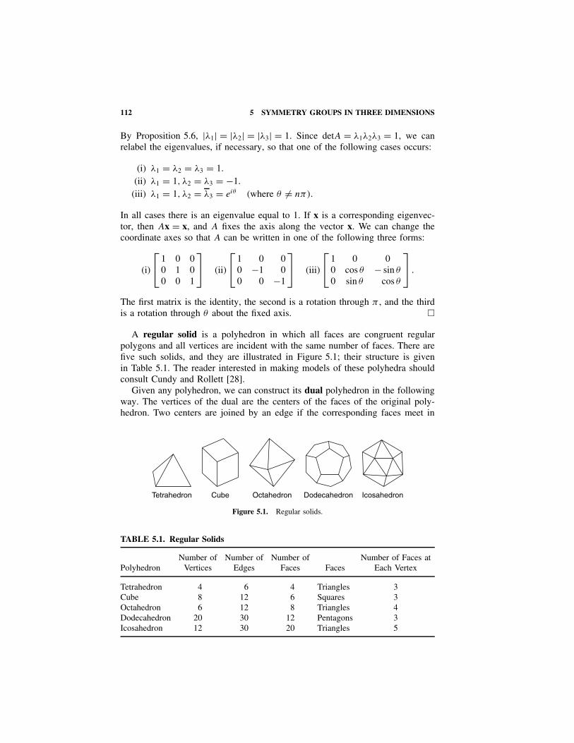
112 5 SYMMETRY GROUPS IN THREE DIMENSIONS
By Proposition 5.6, |λ1| = |λ2| = |λ3| = 1. Since detA = λ1λ2λ3 = 1, we canrelabel the eigenvalues, if necessary, so that one of the following cases occurs:
(i) λ1 = λ2 = λ3 = 1.(ii) λ1 = 1, λ2 = λ3 = −1.
(iii) λ1 = 1, λ2 = λ3 = eiθ (where θ = nπ).
In all cases there is an eigenvalue equal to 1. If x is a corresponding eigenvec-tor, then Ax = x, and A fixes the axis along the vector x. We can change thecoordinate axes so that A can be written in one of the following three forms:
(i)
1 0 0
0 1 00 0 1
(ii)
1 0 0
0 −1 00 0 −1
(iii)
1 0 0
0 cos θ − sin θ
0 sin θ cos θ
.
The first matrix is the identity, the second is a rotation through π , and the thirdis a rotation through θ about the fixed axis. �
A regular solid is a polyhedron in which all faces are congruent regularpolygons and all vertices are incident with the same number of faces. There arefive such solids, and they are illustrated in Figure 5.1; their structure is givenin Table 5.1. The reader interested in making models of these polyhedra shouldconsult Cundy and Rollett [28].
Given any polyhedron, we can construct its dual polyhedron in the followingway. The vertices of the dual are the centers of the faces of the original poly-hedron. Two centers are joined by an edge if the corresponding faces meet in
Tetrahedron Cube Octahedron Dodecahedron Icosahedron
Figure 5.1. Regular solids.
TABLE 5.1. Regular Solids
PolyhedronNumber of
VerticesNumber of
EdgesNumber of
Faces FacesNumber of Faces at
Each Vertex
Tetrahedron 4 6 4 Triangles 3Cube 8 12 6 Squares 3Octahedron 6 12 8 Triangles 4Dodecahedron 20 30 12 Pentagons 3Icosahedron 12 30 20 Triangles 5

PROPER ROTATIONS OF REGULAR SOLIDS 113
an edge. The dual of a regular tetrahedron is another regular tetrahedron. Thedual of a cube is an octahedron, and the dual of an octahedron is a cube. Thedodecahedron and icosahedron are also duals of each other. Any symmetry ofa polyhedron will induce a symmetry on its dual and vice versa. Hence dualpolyhedra will have the same rotation group.
Theorem 5.11. The group of proper rotations of a regular tetrahedron is isomor-phic to A4.
Proof. Label the vertices of the tetrahedron 1, 2, 3, and 4. Then any rotationof the tetrahedron will permute these vertices. So if G is the rotation group of thetetrahedron, we have a group morphism f : G → S4 whose kernel contains onlythe identity element. Hence, by the morphism theorem, G is isomorphic to Imf .
We can use Theorem 4.40 to count the number of elements of G. The stabilizerof the vertex 1 is the set of elements fixing 1 and is {(1), (234), (243)}. The vertex1 can be taken to any of the four vertices under G, so the orbit of 1 is the set offour vertices. Hence |G| = |Stab 1| |Orb 1| = 3.4 = 12.
There are two types of nontrivial elements in G that are illustrated inFigures 5.2 and 5.3. There are rotations of order 3 about axes, each of whichjoins a vertex to the center of the opposite face. These rotations perform an evenpermutation of the vertices because each fixes one vertex and permutes the otherthree cyclically. There are also rotations of order 2 about axes, each of which joinsthe midpoints of a pair of opposite edges. (Two edges in a tetrahedron are saidto be opposite if they do not meet.) The corresponding permutations interchangetwo pairs of vertices and, being products of two transpositions, are even.
Hence Imf consists of 12 permutations, all of which are even, andImf = A4. �
The alternating group A4 is sometimes called the tetrahedral group.There are many different ways of counting the number of elements of the
rotation group G of the tetrahedron. One other way is as follows. Considerthe tetrahedron sitting on a table, and shade in an equilateral triangle on thetable where the bottom face rests, as in Figure 5.4. Any symmetry in G canbe performed by picking up the tetrahedron, turning it, and replacing it on thetable so that one face of the tetrahedron lies on top of the shaded equilateraltriangle. Any of the four faces of the tetrahedron can be placed on the table, andeach face can be placed on top of the shaded triangle in three different ways.
24
31
Figure 5.2. Element (2 3 4).
4
2
3
1
Figure 5.3. Element (1 2) Ž (3 4).
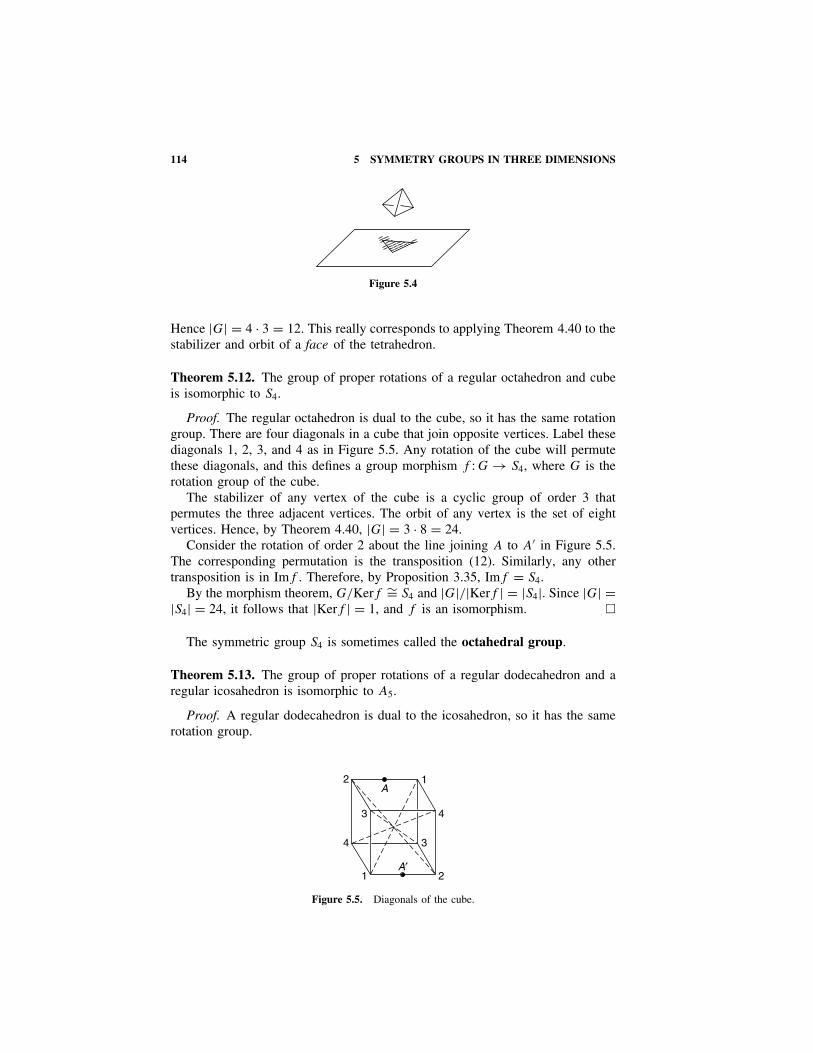
114 5 SYMMETRY GROUPS IN THREE DIMENSIONS
Figure 5.4
Hence |G| = 4 · 3 = 12. This really corresponds to applying Theorem 4.40 to thestabilizer and orbit of a face of the tetrahedron.
Theorem 5.12. The group of proper rotations of a regular octahedron and cubeis isomorphic to S4.
Proof. The regular octahedron is dual to the cube, so it has the same rotationgroup. There are four diagonals in a cube that join opposite vertices. Label thesediagonals 1, 2, 3, and 4 as in Figure 5.5. Any rotation of the cube will permutethese diagonals, and this defines a group morphism f : G → S4, where G is therotation group of the cube.
The stabilizer of any vertex of the cube is a cyclic group of order 3 thatpermutes the three adjacent vertices. The orbit of any vertex is the set of eightvertices. Hence, by Theorem 4.40, |G| = 3 · 8 = 24.
Consider the rotation of order 2 about the line joining A to A′ in Figure 5.5.The corresponding permutation is the transposition (12). Similarly, any othertransposition is in Imf . Therefore, by Proposition 3.35, Imf = S4.
By the morphism theorem, G/Kerf ∼= S4 and |G|/|Kerf | = |S4|. Since |G| =|S4| = 24, it follows that |Kerf | = 1, and f is an isomorphism. �
The symmetric group S4 is sometimes called the octahedral group.
Theorem 5.13. The group of proper rotations of a regular dodecahedron and aregular icosahedron is isomorphic to A5.
Proof. A regular dodecahedron is dual to the icosahedron, so it has the samerotation group.
1
4
3
2
2A′
A
3
4
1
Figure 5.5. Diagonals of the cube.

PROPER ROTATIONS OF REGULAR SOLIDS 115
There are 30 edges of an icosahedron, and there are 15 lines through the centerjoining the midpoints of opposite edges. (The reflection of each edge in the centerof the icosahedron is a parallel edge, called the opposite edge.) Given any oneof these 15 lines, there are exactly two others that are perpendicular both to thefirst line and to each other. We call three such mutually perpendicular lines atriad. The 15 lines fall into five sets of triads. Label these triads 1, 2, 3, 4, and5. Figure 5.6 shows the top half of an icosahedron, where we have labeled theendpoints of each triad. (The existence of mutually perpendicular triads and thelabeling of the diagram can best be seen by actually handling a model of theicosahedron.)
A rotation of the icosahedron permutes the five triads among themselves, andthis defines a group morphism f : G → S5, where G is the rotation group of theicosahedron.
The stabilizer of any vertex of the icosahedron is a group of order 5 thatcyclically permutes the five adjacent vertices. The orbit of any vertex is the setof all 12 vertices. Hence, by Theorem 4.40, |G| = 5 · 12 = 60.
There are three types of nontrivial elements in G. There are rotations of order5 about axes through a vertex. The rotations about the vertex A in Figure 5.6correspond to multiples of the cyclic permutation (12345), all of which are even.There are rotations of order 3 about axes through the center of a face. The rota-tions about an axis through the point B, in Figure 5.6, are multiples of (142)and are therefore even permutations. Finally, there are rotations of order 2 aboutthe 15 lines joining midpoints of opposite edges. The permutation correspond-ing to a rotation about an axis through C, in Figure 5.6, is (23) Ž (45), whichis even.
Every 3-cycle occurs in the image of f so, by Proposition 3.37, Imf = A5.Since G and A5 both have 60 elements, the morphism theorem implies that G isisomorphic to A5. �
The alternating group A5 is sometimes called the icosahedral group.
3
4
3
5
2
1 3
4
1
5
2
24
3
4
21
5
5
A
CB
1
Figure 5.6. Ends of the triads of the icosahedron.

116 5 SYMMETRY GROUPS IN THREE DIMENSIONS
FINITE ROTATION GROUPS IN THREE DIMENSIONS
We now proceed to show that the only finite proper rotation groups in threedimensions are the three symmetry groups of the regular solids, A4, S4, and A5
together with the cyclic and dihedral groups, Cn and Dn.The unit sphere S2 = {x ∈ R3
∣∣ ||x|| = 1} is mapped to itself by every elementof O(3). Every rotation group fixing the origin is determined by its action on theunit sphere S2. By Theorem 5.10, every nonidentity element A ∈ SO(3) leavesprecisely two antipodal points on S2 fixed. That is, there exists x ∈ S2 such thatA(x) = x and A(−x) = −x. The points x and −x are called the poles of A. LetP be the set of poles of the nonidentity elements of a finite subgroup G of SO(3).
Proposition 5.14. G acts on the set, P , of poles of its nonidentity elements.
Proof. We show that G permutes the poles among themselves. Let A, B, benonidentity elements of G, and let x be a pole of A. Then (BAB−1)B(x) =BA(x) = B(x), so that B(x) is a pole of BAB−1. Therefore, the image of anypole is another pole, and G acts on the set of poles. �
We classify the rotation groups by considering the number of elements in thestabilizers and orbits of the poles. Recall that the stabilizer of a pole x, Stab x ={A ∈ G|A(x) = x}, is a subgroup of G, and that the orbit of x, Orb x = {B(x)|B ∈G}, is a subset of the set P of poles. In Table 5.2 we look at the stabilizers andorbits of the poles of the rotation groups we have already discussed.
TABLE 5.2. Poles of the Finite Rotation Groups
Group G =|G | =
Symmetries of
Cnnn-agonal cone
Looking downon the pole, x
Dn2nn-agonal cylinder
A412tetrahedron
n1
212
38
46
or or or
230
512
or or
320
or
n1
2n
2n
n2
26
34
34
|Stab x| =|Orb x| =
Group G =|G | =
Symmetries of
S424cube
Looking downon the pole, x
A560dodecahedron or icosahedronor octahedron
|Stab x| =|Orb x| =

FINITE ROTATION GROUPS IN THREE DIMENSIONS 117
p
x
2p
34p
3or
x
p
2por
x
x x x
Rotation:
Looking down onthe pole x:
Order of the rotation: 2 3 4 or 2
Figure 5.7. Rotations of the cube.
We take Cn to be the rotation group of a regular n-agonal cone whose baseis a regular n-gon. (The sloping edges of the cone must not be equal to the baseedges if n = 3.) Dn is the rotation group of a regular n-agonal cylinder whosebase is a regular n-gon. (The vertical edges must not be equal to the base edgesif n = 4.)
Each stabilizer group, Stab x, is a cyclic subgroup of rotations of the solidabout the axis through x. The orbit of x, Orb x, is the set of poles of the sametype as x. As a check on the number of elements in the stabilizers and orbits, wehave |G| = |Stab x||Orb x| for each pole x.
For example, the cube has three types of poles and four types of nontrivialelements in its rotation group; these are illustrated in Figure 5.7.
Theorem 5.15. Any finite subgroup of SO(3) is isomorphic to one of
Cn(n � 1), Dn(n � 2), A4, S4 or A5.
Proof. Let G be a finite subgroup of SO(3). Choose a set of poles x1, . . . , xr ,one from each orbit. Let pi = |Stab xi | and qi = |Orb xi |, so that piqi = n = |G|.
Each nonidentity element of G has two poles; thus the total number of poles,counting repetitions, is 2(n − 1). The pole xi occurs as a pole of a nonidentityelement pi − 1 times. There are qi poles of the same type as xi . Therefore, thetotal number of poles, counting repetitions, is
2(n − 1) =r∑
i=1
qi(pi − 1) =r∑
i=1
(n − qi),
so
2 − 2
n=
r∑i=1
(1 − 1
pi
). (∗)

118 5 SYMMETRY GROUPS IN THREE DIMENSIONS
If G is not the trivial group, n � 2 and 1 � 2 − 2
n< 2. Since xi is a pole of
some nonidentity element, Stab xi contains a nonidentity element, and pi � 2.
Therefore,1
2� 1 − 1
pi
< 1. It follows from (*) that the number of orbits, r , must
be 2 or 3.If there are just two orbits, it follows that
2 − 2
n= 1 − 1
p1+ 1 − 1
p2
and 2 = n
p1+ n
p2= q1 + q2. Hence q1 = q2 = 1, and p1 = p2 = n. This means
that x1 = x2, and there is just one axis of rotation. Therefore, G is isomorphicto the cyclic group Cn.
If there are three orbits, it follows that
2 − 2
n= 1 − 1
p1+ 1 − 1
p2+ 1 − 1
p3
1 + 2
n= 1
p1+ 1
p2+ 1
p3. (**)
Suppose that p1 � p2 � p3. If p1 � 3, we would have
1
p1+ 1
p2+ 1
p3� 1
3+ 1
3+ 1
3= 1,
which is a contradiction, since2
n> 0. Hence p1 = 2 and q1 = n
2.
Now 1 + 2
n= 1
2+ 1
p2+ 1
p3, so
1
2+ 2
n= 1
p2+ 1
p3. If p2 � 4, we would
have1
p2+ 1
p3� 1
4+ 1
4= 1
2, which is a contradiction, since
2
n> 0. Hence p2
is 2 or 3. The only possibilities are the following.
Case (i). p1 = 2, p2 = 2, p3 = n
2, n is even and n � 4, q1 = n
2, q2 = n
2, and
q3 = 2.Case (ii). p1 = 2, p2 = 3, p3 = 3, n = 12, q1 = 6, q2 = 4, and q3 = 4.Case (iii). p1 = 2, p2 = 3, p3 = 4, n = 24, q1 = 12, q2 = 8, and q3 = 6.Case (iv). p1 = 2, p2 = 3, p3 = 5, n = 60, q1 = 30, q2 = 20, and q3 = 12.
If p2 = 2 and p3 � 6,1
p2+ 1
p3� 1
3+ 1
6= 1
2, which contradicts (**), since
2
n> 0.

FINITE ROTATION GROUPS IN THREE DIMENSIONS 119
Case (i). Let H = Stab x3. This is a group of rotations about one axis, and itis a cyclic group of order n/2. Any other element A that is not in H is oforder 2 and is a half turn. Therefore, G = H ∪ HA, and G is isomorphicto Dn/2 of order n.
Case (ii). Let y1, y2, y3, and y4 be the four poles in Orb x2. Now p2 =|Stab yi | = 3; thus Stab y1 permutes y2, y3, and y4 as in Figure 5.8. There-fore, ||y2 − y1|| = ||y3 − y1|| = ||y4 − y1||. We have similar results for Staby2 and Stab y3. Hence y1, y2, y3, and y4 are the vertices of a regular tetra-hedron, and G is a subgroup of the symmetries of this tetrahedron. Since|G| = 12, G must be the whole rotation group, A4.
Case (iii). Let y1, y2, . . . , y6 be the six poles in Orb x3. Since p3 = 4, a rota-tion in Stab yi must fix two of the poles and rotate the other four cyclically.Hence y1, y2, . . . , y6 must lie at the vertices of a regular octahedron. Again,since |G| = 24, G must be the whole rotation group, S4, of this octahedron.
Case (iv). Let y1, y2, . . . , y12 be the 12 poles in Orb x3. Any element oforder 5 in G must permute these poles and hence must fix two polesand permute the others, as in Figure 5.9, in two disjoint 5-cycles, say(
2 3 4 5 6)
Ž(
7 8 9 10 11), where we denote the pole yi
by i. The points y2, y3, y4, y5, and y6 form a regular pentagon and theirdistances from y1 are all equal. Using similar results for rotations of order5 about the other poles, we see that the poles are the vertices of anicosahedron, and the group G is the proper rotation group, A5, of thisicosahedron. �
Throughout this section we have considered only proper rotations. However,if we allow improper rotations as well, it can be shown that a finite subgroup
y2
y3
y1
y4Stab y1
Figure 5.8
1
2
3
4
5
6
7
8
9
10
1112
Stab y1
Figure 5.9
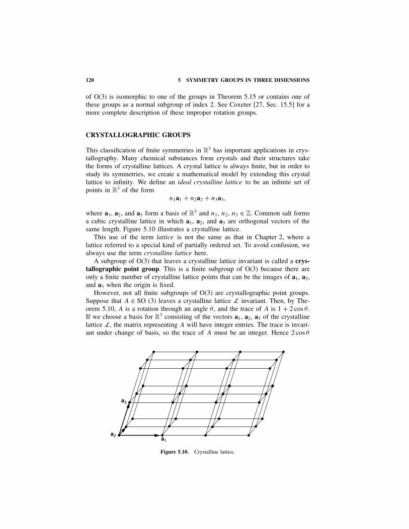
120 5 SYMMETRY GROUPS IN THREE DIMENSIONS
of O(3) is isomorphic to one of the groups in Theorem 5.15 or contains one ofthese groups as a normal subgroup of index 2. See Coxeter [27, Sec. 15.5] for amore complete description of these improper rotation groups.
CRYSTALLOGRAPHIC GROUPS
This classification of finite symmetries in R3 has important applications in crys-tallography. Many chemical substances form crystals and their structures takethe forms of crystalline lattices. A crystal lattice is always finite, but in order tostudy its symmetries, we create a mathematical model by extending this crystallattice to infinity. We define an ideal crystalline lattice to be an infinite set ofpoints in R3 of the form
n1a1 + n2a2 + n3a3,
where a1, a2, and a3 form a basis of R3 and n1, n2, n3 ∈ Z. Common salt formsa cubic crystalline lattice in which a1, a2, and a3 are orthogonal vectors of thesame length. Figure 5.10 illustrates a crystalline lattice.
This use of the term lattice is not the same as that in Chapter 2, where alattice referred to a special kind of partially ordered set. To avoid confusion, wealways use the term crystalline lattice here.
A subgroup of O(3) that leaves a crystalline lattice invariant is called a crys-tallographic point group. This is a finite subgroup of O(3) because there areonly a finite number of crystalline lattice points that can be the images of a1, a2,and a3 when the origin is fixed.
However, not all finite subgroups of O(3) are crystallographic point groups.Suppose that A ∈ SO (3) leaves a crystalline lattice L invariant. Then, by The-orem 5.10, A is a rotation through an angle θ , and the trace of A is 1 + 2 cos θ .If we choose a basis for R3 consisting of the vectors a1, a2, a3 of the crystallinelattice L, the matrix representing A will have integer entries. The trace is invari-ant under change of basis, so the trace of A must be an integer. Hence 2 cos θ
a3
a2a1
Figure 5.10. Crystalline lattice.

EXERCISES 121
must be integral, and θ must be either kπ/2 or kπ/3, where k ∈ Z. It followsthat every element of a crystallographic point group in SO(3) can only containelements of order 1, 2, 3, 4, or 6.
It can be shown that every crystallographic point group in SO(3) is isomorphicto one of C1, C2, C3, C4, C6, D2, D3, D4, D6, A4, or S4.
If we allow reflections, the only other such groups in O(3) must contain oneof these groups as a normal subgroup of index 2. Every one of these groupsoccurs in nature as the point group of at least one chemical crystal. See Coxeter[27, Sec. 15.6] or Lomont [31, Chap. 4, Sec. 4].
EXERCISES
Find the group of proper rotations and the group of all rotations of the figures inExercises 5.1 to 5.7.
5.1. 5.2. 5.3. 5.4.
5.5. 5.6. 5.7.
5.8. Let G be the subgroup of O(2) isomorphic to Dn. Find two matrices A andB so that any element of G can be written as a product of A’s and B’s.
5.9. What is the group of proper rotations of a rectangular box of length 3 cm,depth 2 cm, and height 2 cm?
Find the proper rotation group of the 13 Archimedean solids in Exercises 5.10to 5.22. All the faces of these solids are regular polygons and all the vertices aresimilar. (See Cundy and Rollet [28] for methods on how to construct these solids.)
5.10. 5.11. 5.12. 5.13.
5.14. 5.15. 5.16.
5.17. 5.18. 5.19.

122 5 SYMMETRY GROUPS IN THREE DIMENSIONS
5.20. 5.21. 5.22.
5.23. It is possible to inscribe five cubes in a regular dodecahedron. One suchcube is shown in Figure 5.11. Use these cubes to show that the rotationgroup of the dodecahedron is A5.
Figure 5.11. Cube inside a dodecahedron.
5.24. What is the proper symmetry group of a cube in which three faces, comingtogether at one vertex, are painted green and the other faces are red?
5.25. Find the group of all rotations (both proper and improper) of a regulartetrahedron.
5.26. Let G be the full symmetry group of the cube. Define f : G → S4 as inTheorem 5.12. Find the kernel of f and the order of G.
5.27. Let the vertices of a tetrahedron be (1, 1, 1), (−1, −1, 1), (−1, 1,−1),and (1, −1, −1). Find matrices in SO(3) of orders 2 and 3 that leave thetetrahedron invariant.
5.28. Let the vertices of a cube be (±1, ±1, ±1). Find matrices in SO(3) oforders 2, 3, and 4 that leave the cube invariant.
Find the symmetry groups of the chemical molecules in Exercises 5.29 to 5.31.(Assume that all of the C-C bonds are equivalent.)
5.29.
C C
C
CC
CH H
HH
H H
Benzene
5.30.
C C
C
CC
CH H
CH3CH3
H H
Xylene
5.31.
C C
C
CC
CNO2 CH3
NO2H
H NO2
Trinitrotoluene (TNT)
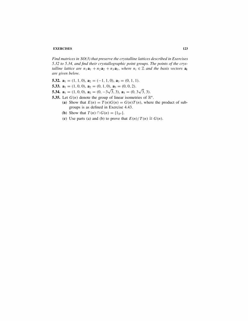
EXERCISES 123
Find matrices in SO(3) that preserve the crystalline lattices described in Exercises5.32 to 5.34, and find their crystallographic point groups. The points of the crys-talline lattice are n1 a1 + n2 a2 + n3 a3 , where ni ∈ Z and the basis vectors ai
are given below.
5.32. a1 = (1, 1, 0), a2 = (−1, 1, 0), a3 = (0, 1, 1).5.33. a1 = (1, 0, 0), a2 = (0, 1, 0), a3 = (0, 0, 2).5.34. a1 = (1, 0, 0), a2 = (0, −3
√3, 3), a3 = (0, 3
√3, 3).
5.35. Let G(n) denote the group of linear isometries of Rn.(a) Show that E(n) = T (n)G(n) = G(n)T (n), where the product of sub-
groups is as defined in Exercise 4.43.(b) Show that T (n) ∩ G(n) = {1Rn}.(c) Use parts (a) and (b) to prove that E(n)/T (n) ∼= G(n).

6POLYA–BURNSIDE METHODOF ENUMERATION
This chapter provides an introduction to the Polya–Burnside method of countingthe number of orbits of a set under the action of a symmetry group. If a groupG acts on a set X and we know the number of elements of X, this method willenable us to count the number of different types of elements of X under theaction of G.
For example, how many different chemical compounds can be obtained byattaching a CH3 or H radical to each carbon atom in the benzene ring ofFigure 6.3? There are 26 different ways of attaching a CH3 or H radical on paper,but these do not all give rise to different compounds because many are equivalentunder a symmetry. There are six different ways of attaching one CH3 radical andfive H radicals, but they all give rise to the same compound. The dihedral groupD6 acts on the 26 ways of attaching the radicals, and the number of differentcompounds is the number of orbits under the action of D6, that is, the number offormulas that cannot be obtained from each other by any rotation or reflection.
We have seen that the number of different switching circuits that can beobtained with n switches is 22n
. This number grows very quickly as n becomeslarge. Table 2.11 gives the 16 switching functions of two variables; when n = 3,there are 256 different circuits, and when n = 4, there are 65,536 different cir-cuits. However, many of these circuits are equivalent if we change the labels ofthe switches. That is, the symmetric group, Sn, acts on the 22n
different circuitsby permuting the labels of the switches. The number of nonequivalent circuits isthe number of orbits under the action of Sn.
BURNSIDE’S THEOREM
Let G be a finite group that acts on a finite set X. The following theoremdescribes the number of orbits in terms of the number of elements left fixed
Modern Algebra with Applications, Second Edition, by William J. Gilbert and W. Keith NicholsonISBN 0-471-41451-4 Copyright 2004 John Wiley & Sons, Inc.
124

BURNSIDE’S THEOREM 125
by each element of G. It was first proved by W. Burnside in 1911 and wascalled Burnside’s lemma; it was not until 1937 that its applicability to manycombinatorial problems was discovered by G. Polya.
Theorem 6.1. Burnside’s Theorem. Let G be a finite group that acts on theelements of a finite set X. For each g ∈ G, let Fix g = {x ∈ X|g(x) = x}, theset of elements of X left fixed by g. If N is the number of orbits of X underG, then
N = 1
|G|∑g∈G
| Fix g|.
Proof. We count the set S = {(x, g) ∈ X × G|g(x) = x} in two different ways.Consider Table 6.1, whose columns are indexed by the elements of X and whoserows are indexed by the elements of G. Put a value of 1 in the (x, g) position ifg(x) = x; otherwise, let the entry be 0.
The sum of the entries in row g is the number |Fix g| of elements left fixedby g. The sum of the entries in column x is |Stab x|, the number of elements ofG that fix x.
We can count the number of elements of S either by totaling the row sums orby totaling the column sums. Hence
|S| =∑g∈G
|Fix g| =∑x∈X
|Stab x|.
Choose a set of representatives, x1, x2, . . . , xN , one from each orbit of X underG. If x is in the same orbit as xi , then Orb x = Orb xi , and by Theorem 4.40,|Stab x| = |Stab xi |. Hence
∑g∈G
|Fix g| =N∑
i=1
·∑x∈Orb xi
|Stab x| =N∑
i=1
|Orb xi ||Stab xi | = N · |G|
by Theorem 4.40. The theorem now follows. �
TABLE 6.1. Elements of S Correspond to the 1’s inThis Table
Elements of X Row
x Sums↓
...
1Elements g . . .1 0 1 1 1 0. . . |Fix g|
of G 0...
Column → |Stab x|Sums
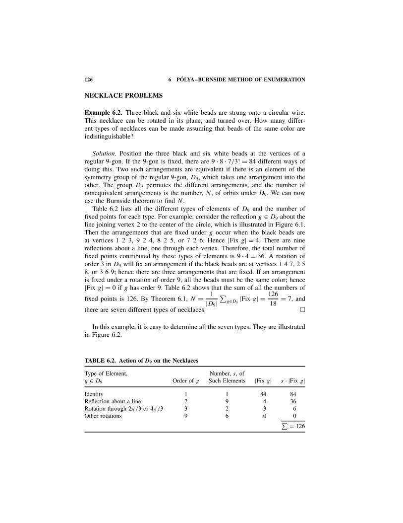
126 6 POLYA–BURNSIDE METHOD OF ENUMERATION
NECKLACE PROBLEMS
Example 6.2. Three black and six white beads are strung onto a circular wire.This necklace can be rotated in its plane, and turned over. How many differ-ent types of necklaces can be made assuming that beads of the same color areindistinguishable?
Solution. Position the three black and six white beads at the vertices of aregular 9-gon. If the 9-gon is fixed, there are 9 · 8 · 7/3! = 84 different ways ofdoing this. Two such arrangements are equivalent if there is an element of thesymmetry group of the regular 9-gon, D9, which takes one arrangement into theother. The group D9 permutes the different arrangements, and the number ofnonequivalent arrangements is the number, N , of orbits under D9. We can nowuse the Burnside theorem to find N .
Table 6.2 lists all the different types of elements of D9 and the number offixed points for each type. For example, consider the reflection g ∈ D9 about theline joining vertex 2 to the center of the circle, which is illustrated in Figure 6.1.Then the arrangements that are fixed under g occur when the black beads areat vertices 1 2 3, 9 2 4, 8 2 5, or 7 2 6. Hence |Fix g| = 4. There are ninereflections about a line, one through each vertex. Therefore, the total number offixed points contributed by these types of elements is 9 · 4 = 36. A rotation oforder 3 in D9 will fix an arrangement if the black beads are at vertices 1 4 7, 2 58, or 3 6 9; hence there are three arrangements that are fixed. If an arrangementis fixed under a rotation of order 9, all the beads must be the same color; hence|Fix g| = 0 if g has order 9. Table 6.2 shows that the sum of all the numbers of
fixed points is 126. By Theorem 6.1, N = 1
|D9|∑
g∈D9|Fix g| = 126
18= 7, and
there are seven different types of necklaces. �
In this example, it is easy to determine all the seven types. They are illustratedin Figure 6.2.
TABLE 6.2. Action of D9 on the Necklaces
Type of Element,g ∈ D9 Order of g
Number, s, ofSuch Elements |Fix g| s · |Fix g|
Identity 1 1 84 84Reflection about a line 2 9 4 36Rotation through 2π/3 or 4π/3 3 2 3 6Other rotations 9 6 0 0∑ = 126

NECKLACE PROBLEMS 127
12
3
4
56
7
8
9
g
Figure 6.1. D9 acting on the necklace.
Figure 6.2. Seven types of necklaces.
C C
C
CC
C4 1
65
3 2
– – – – – – – – – – –g
Figure 6.3. Benzene ring.
TABLE 6.3. Action of D6 on the Compounds
Type of Element,g ∈ D6 Order of g
Number, s, ofSuch Elements |Fix g| s · |Fix g|
Identity 1 1 26 64Reflection in a line through
opposite vertices[e.g., (26) Ž (35) Ž (1) Ž (4)]
2 3 24 48
Reflection in a line throughmidpoints of opposite sides[e.g., (56) Ž (14) Ž (23)]
2 3 23 24
Rotation through ±π/3[e.g., (123456)]
6 2 2 4
Rotation through ±2π/3[e.g., (135) Ž (246)]
3 2 22 8
Rotation through π ,(14) Ž (25) Ž (36)
2 1 23 8
|D6| = 12∑ = 156

128 6 POLYA–BURNSIDE METHOD OF ENUMERATION
Example 6.3. Find the number of different chemical compounds that can beobtained by attaching CH3 or H radicals to a benzene ring.
Solution. The carbon atoms are placed at the six vertices of a regular hexagon,and there are 26 ways of attaching CH3 or H radicals. The dihedral group D6
acts on these 26 ways, and we wish to find the number of orbits.Consider a reflection, g, about a line through opposite vertices. The order of
g is 2, and there are three such reflections, through the three opposite pairs ofvertices. |Fix g| can be determined by looking at Figure 6.3. If a configuration isfixed by g, the radical in place 2 must be the same as the radical in place 6, andalso the radicals in places 3 and 5 must be equal. Hence the radicals in places 1,2, 3, and 4 can be chosen arbitrarily, and this can be done in 24 ways.
The number of configurations left fixed by each element of D6 is given inTable 6.3. To check that we have not omitted any elements, we add the columncontaining the numbers of elements, and this should equal the order of the groupD6. It follows from the Burnside theorem that the number of orbits is 156/|D6| =156/12 = 13. Hence there are 13 different types of molecules obtainable. �
COLORING POLYHEDRA
Example 6.4. How many ways is it possible to color the vertices of a cube if n
colors are available?
Solution. If the cube is fixed, the eight vertices can each be colored in n ways,giving a total of n8 colorings. The rotation group of the cube, S4, permutes thesecolorings among themselves, and the number of orbits is the number of distinctcolorings taking the rotations into account. We can calculate the number of orbitsusing the Burnside theorem.
There are five types of elements in the rotation group of the cube. We take anelement g of each type and determine the vertices that must have the same colorin order that the coloring be invariant under g.
Figure 6.4 illustrates the different types of rotations; vertices that have to havethe same color are shaded in the same way. Table 6.4 gives the number of fixedcolorings, with column totals.
By the Burnside theorem, the number of orbits and hence the number ofcolorings is
1
|S4|∑g∈S4
|Fix g| = 124 (n8 + 17n4 + 6n2).
p
g1
2p/3
g2p/2
g3p
g4
Figure 6.4. Types of rotations of the cube.

COLORING POLYHEDRA 129
TABLE 6.4. Colorings of the Vertices of the Cube
Type ofElement, gi
(Figure 6.4)Order of
gi
Number,s, of
Such Elements
Number,r , of Choices
of Colors
|Fix gi |Which Is
nr s · |Fix gi |Identity 1 1 8 n8 n8
g1 2 6 · 1 = 6 4 n4 6n4
g2 3 4 · 2 = 8 4 n4 8n4
g3 4 3 · 2 = 6 2 n2 6n2
g4 2 3 · 1 = 3 4 n4 3n4
|S4| = 24 n8 + 17n4 + 6n2
This shows, incidentally, that n8 + 17n4 + 6n2 is divisible by 24 for alln ∈ P. �
Example 6.5. In how many ways is it possible to color a regular dodecahedronso that five of its faces are black and the other seven are white?
Solution. The number of ways† of choosing five faces of a fixed dodecahedron
to be colored black is
(125
)= 12 · 11 · 10 · 9 · 8
5!= 792.
The different types of elements in the rotation group, A5, of the dodecahedronare shown in Figure 6.5. The numbers of elements of a given type, in Table 6.5,are calculated as follows. An element of order 3 is a rotation about an axisthrough opposite vertices. Since there are 20 vertices, there are ten such axes.There are two nonidentity rotations of order 3 about each axis; thus the totalnumber of elements of order 3 is 10 · 2 = 20. The elements of orders 2 and 5can be counted in a similar way.
If g2 ∈ A5 is of order 3, we can calculate |Fix g2| as follows. The elementg2 does not fix any face and permutes the faces in disjoint 3-cycles. Now fiveblack faces cannot be permuted by disjoint 3-cycles without fixing two faces, so|Fix g2| = 0. Similarly, |Fix g1| = 0 if g1 is a 2-cycle. If g3 is of order 5, theng3 is a rotation about an axis through the centers of two opposite faces, and thesetwo faces are fixed. The other ten faces are permuted in two disjoint 5-cycles;either of these 5-cycles can be black; thus |Fix g3| = 2.
It follows from Table 6.5 and from the Burnside theorem that the number ofdifferent colorings is 840/60 = 14. �
Any face coloring of the dodecahedron corresponds to a vertex coloring of itsdual, the icosahedron.
† A set of n elements has
(n
k
)subsets of k � n elements where
(n
k
)= n!
k!(n − k)!is the binomial
coefficient.

130 6 POLYA–BURNSIDE METHOD OF ENUMERATION
g1 g2 g3
Figure 6.5. Types of rotations of a dodecahedron.
TABLE 6.5. Colorings of the Dodecahedron
Type of Element, gi
(Figure 6.5) Order of gi
Number, s, ofSuch Elements |Fix gi | s · |Fix gi |
Identity 1 1 792 792g1 2 15 0 0g2 3 10 · 2 = 20 0 0g3 5 6 · 4 = 24 2 48
|A5| = 60∑ = 840
COUNTING SWITCHING CIRCUITS
The Burnside theorem can still be applied when the sets to be enumerated do nothave any geometric symmetry. In this case, the symmetry group is usually thefull permutation group Sn.
Consider the different switching circuits obtained by using three switches. Wecan think of these as black boxes with three binary inputs x1, x2, and x3 and onebinary output f (x1, x2, x3), as in Figure 6.6. Two circuits, f and g, are calledequivalent if there is a permutation π of the variables so that f (x1, x2, x3) =g(xπ1, xπ2, xπ3). Equivalent circuits can be obtained from each other by justpermuting the wires outside the black boxes, as in Figure 6.7.
x1
x2
x3
f f (x1, x2, x3)
Figure 6.6. Switching circuit.
f f (x2, x3, x1)
x1
x2
x3
Figure 6.7. Permutation of the inputs.

COUNTING SWITCHING CIRCUITS 131
Example 6.6. Find the number of switching circuits using three switches thatare not equivalent under permutations of the inputs.
Solution. There are eight possible inputs using three binary variables andhence there are 28 = 256 circuits to consider. The symmetric group S3 actson these 256 circuits, and we wish to find the number of different equivalenceclasses, that is, the number of orbits.
Table 6.6 lists the number of circuits left fixed by the different types of ele-ments in S3. For example, if the switching function f (x1, x2, x3) is fixed bythe transposition (12) of the input variables, then f (0, 1, 0) = f (1, 0, 0) andf (0, 1, 1) = f (1, 0, 1). The values of f for the inputs (0, 0, 0), (0, 0, 1), (0, 1,0), (0, 1, 1), (1, 1, 0), and (1, 1, 1) can be chosen arbitrarily in 26 ways.
By Burnside’s theorem and Table 6.6, the number of nonequivalent circuits is480/|S3| = 480/6 = 80. �
However, this number can be reduced further if we allow permutations andcomplementation of the three variables. In a circuit consisting of two-state switches,the variable xi can be complemented by simply reversing each of the switchescontrolled by xi . The resulting circuit is just as simple and the cost is the same asthe original one. In transistor networks, we can just permute the input wires andadd NOT gates as in Figure 6.8.
The eight input values of a three-variable switching circuit can be consideredas the vertices of a three-dimensional cube, as shown in Figure 6.9. The six facesof this cube are defined by the equations x1 = 0, x1 = 1, x2 = 0, x2 = 1, x3 = 0,x3 = 1. The group that permutes and complements the variables takes each faceto another face and takes opposite faces to opposite faces. Hence the group is thecomplete symmetry group, G, of the cube. There is a morphism ψ : G → {1, −1},
TABLE 6.6. Action of S3 on the Inputs of the Switches
Type of Element,g ∈ S3
Number, s, ofSuch Elements |Fix g| s · |Fix g|
Identity 1 28 28 = 256Transposition 3 26 3 · 26 = 1923-Cycle 2 24 2 · 24 = 32
|S3| = 6 480
f f (x2, x1′, x3′ )x3
x2
x1
NOT
NOT
Figure 6.8. Permutation and complementation of inputs.
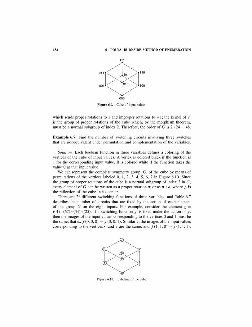
132 6 POLYA–BURNSIDE METHOD OF ENUMERATION
111
011
001
000
010
101110
100
Figure 6.9. Cube of input values.
which sends proper rotations to 1 and improper rotations to −1; the kernel of ψ
is the group of proper rotations of the cube which, by the morphism theorem,must be a normal subgroup of index 2. Therefore, the order of G is 2 · 24 = 48.
Example 6.7. Find the number of switching circuits involving three switchesthat are nonequivalent under permutation and complementation of the variables.
Solution. Each boolean function in three variables defines a coloring of thevertices of the cube of input values. A vertex is colored black if the function is1 for the corresponding input value. It is colored white if the function takes thevalue 0 at that input value.
We can represent the complete symmetry group, G, of the cube by means ofpermutations of the vertices labeled 0, 1, 2, 3, 4, 5, 6, 7 in Figure 6.10. Sincethe group of proper rotations of the cube is a normal subgroup of index 2 in G,every element of G can be written as a proper rotation π or as π Ž ρ, where ρ isthe reflection of the cube in its center.
There are 28 different switching functions of three variables, and Table 6.7describes the number of circuits that are fixed by the action of each elementof the group G on the eight inputs. For example, consider the element g =(01) Ž (67) Ž (34) Ž (25). If a switching function f is fixed under the action of g,then the images of the input values corresponding to the vertices 0 and 1 must bethe same; that is, f (0, 0, 0) = f (0, 0, 1). Similarly, the images of the input valuescorresponding to the vertices 6 and 7 are the same, and f (1, 1, 0) = f (1, 1, 1).
3
7
65
21
0
4
Figure 6.10. Labeling of the cube.

COUNTING SWITCHING CIRCUITS 133
TABLE 6.7. Symmetries of a Cube Acting on the Three-VariableSwitching Functions
Type of Element,g, in the SymmetryGroup of the Cube Order of g
Number, s, ofSuch Elements |Fix g| s · |Fix g|
Proper rotations
Identity 1 1 28 256Rotation about a line joining
midpoints of opposite edges[e.g., (01) Ž (67) Ž (34) Ž (25)]
2 6 24 96
Rotation about a line joiningopposite vertices[e.g., (124) Ž (365) Ž (0) Ž (7)]
3 8 24 128
Rotation about a line joining centersof opposite faces[e.g., (0264) Ž (1375)]
4 6 22 24
Rotation about a line joining centersof opposite faces[e.g., (06) Ž (24) Ž (17) Ž (35)]
2 3 24 48
Improper rotations
Reflection in the center[ρ = (07) Ž (16) Ž (25) Ž (34)]
2 1 24 16
Reflection in a diagonal plane[e.g., (01) Ž (67) Ž (34) Ž (25) Ž ρ =(06) Ž (17) Ž (2) Ž (3) Ž (4) Ž (5)]
2 6 26 384
Reflection and rotation[e.g., (124) Ž (365) Ž ρ =(07) Ž (154623)]
6 8 22 32
Reflection and rotation[e.g., (0264) Ž (1375) Ž ρ =(0563) Ž (1472)]
4 6 22 24
Reflection in a central plane[e.g., (06) Ž (24) Ž (17) Ž (35) Ž ρ =(01) Ž (23) Ž (45) Ž (67)]
2 3 24 48
|G| = 48 1056
Also, f (0, 1, 1) = f (1, 0, 0) and f (0, 1, 0) = f (1, 0, 1). Hence the values off (0, 0, 0), f (1, 1, 0), f (0, 1, 1), and f (0, 1, 0) can be chosen arbitrarily in 24
ways, and |Fix g| = 24. In general, if the function f is fixed under g, the imagesof the input values, corresponding to the vertices in any one cycle of g, must bethe same. Hence |Fix g| is 2r , where r is the number of disjoint cycles in thepermutation representation of g.
It follows from Table 6.7 and the Burnside theorem that the number of non-equivalent circuits is 1056/|G| = 1056/48 = 22. �

134 6 POLYA–BURNSIDE METHOD OF ENUMERATION
TABLE 6.8. Number of Types of Switching Functions
Number of Switches, n 1 2 3 4 5
Number of booleanfunctions, 22n
4 16 256 65,536 4,294,967,296
Nonequivalent functionsunder permutations ofinputs
4 12 80 3,984 37,333,248
Nonequivalent functionsunder permutation andcomplementation ofinputs
3 6 22 402 1,228,158
Nonequivalent functionsunder permutation andcomplementation ofinputs and outputs
2 4 14 222 616,126
We can reduce this number slightly more by complementing the function aswell as the variables; this corresponds to adding a NOT gate to the output. Thegroup acting is now a combination of a cyclic group of order 2 with the completesymmetry groups of the cube.
The numbers of nonequivalent circuits for five or fewer switches given inTable 6.8 can be computed as in Example 6.7.
In 1951, the Harvard Computing Laboratory laboriously calculated all thenonequivalent circuits using four switches and the best way to design each ofthem. It was not until later that it was realized that the Polya theory could beapplied to this problem.
In many examples, it is quite difficult to calculate |Fix g| for every elementg of the group G. Polya’s most important contribution to this theory of enumer-ation was to show how |Fix g| can be calculated, using what are called cycleindex polynomials. This saves much individual calculation, and the results onnonequivalent boolean functions in Table 6.8 can easily be calculated. However,it is still a valuable exercise to tackle a few enumeration problems without usingcycle index polynomials, since this gives a better understanding of the Polyatheory. For example, we see in Tables 6.3, 6.4, and 6.7 that |Fix g| is always ofthe form nr , where r is the number of disjoint cycles in g.
Further information on the Polya theory can be obtained from Biggs [15], Lidland Pilz [10], or Stone [22].

EXERCISES 135
EXERCISES
Find the number of different types of circular necklaces that could be made fromthe sets of beads described in Exercises 6.1 to 6.4, assuming that all the beadsare used on one necklace.
6.1. Three black and three white beads.6.2. Four black, three white, and one red bead.6.3. Seven black and five white beads.6.4. Five black, six white, and three red beads.6.5. How many different circular necklaces containing ten beads can be made
using beads of at most two colors?6.6. Five neutral members and two members from each of two warring factions
are to be seated around a circular armistice table. In how many nonequiv-alent ways, under the action of D9, can they be seated if no two membersof opposing factions sit next to each other?
6.7. How many different chemical compounds can be made by attaching H,CH3, C2H5, or Cl radicals to the four bonds of a carbon atom? The radicalslie at the vertices of a regular tetrahedron, and the group is the tetrahedralgroup A4.
6.8. How many different chemical compounds can be made by attaching H,CH3, or OH radicals to each of the carbon atoms in the benzene ring ofFigure 6.3? (Assume that all of the C–C bonds in the ring are equivalent.)
6.9. How many ways can the vertices of a cube be colored using, at most,three colors?
6.10. How many ways can the vertices of a regular tetrahedron be colored using,at most, n colors?
6.11. How many different tetrahedra can be made from n types of resistors wheneach edge contains one resistor?
6.12. How many ways can the faces of a regular dodecahedron be colored using,at most, n colors?
Find the number of different colorings of the faces of the solids described inExercises 6.13 to 6.16.
6.13. A regular tetrahedron with two white faces and two black faces.6.14. A cube with two white, one black, and three red faces.6.15. A regular icosahedron with four black faces and 16 white faces.6.16. A regular dodecahedron with five black faces, two white faces, and five
green faces.6.17. How many ways can the faces of a cube be colored with six different
colors, if all the faces are to be a different color?6.18. (a) Find the number of binary relations, on a set with four elements, that
are not equivalent under permutations of the four elements.

136 6 POLYA–BURNSIDE METHOD OF ENUMERATION
Switchingdevice
Output
Input plug
x1x2x3
Figure 6.11 Figure 6.12
(b) Find the number of equivalence relations, on a set with four elements,that are not equivalent under permutations of the four elements.
6.19. How many different patchwork quilts, four patches long and three patcheswide, can be made from five red and seven blue squares, assuming that thequilts cannot be turned over?
6.20. If the quilts in Exercise 6.19 could be turned over, how many differentpatterns are possible?
6.21. Find the number of ways of distributing three blue balls, two red balls, andfour green balls into three piles.
6.22. If the cyclic group Cn, generated by g, operates on a set S, show that thenumber of orbits is
1
n
∑d/n
|Fix gn/d | · φ(d),
where the Euler φ-function, φ(d), is the number of integers from 1 to d
that are relatively prime to d . (See Exercises 4.55 and 4.56.)6.23. Some transistor switching devices are sealed in a can with three input
sockets at the vertices of an equilateral triangle. The three input wiresare connected to a plug that will fit into the input sockets as shown inFigure 6.11. How many different cans are needed to produce any booleanfunction of three input variables?
6.24. How many different ways can the elements of the poset in Figure 6.12 becolored using, at most, n colors?
6.25. Verify that the number of nonequivalent switching functions of four vari-ables, under permutation of the inputs, is 3984.

7MONOIDS AND MACHINES
For many purposes, a group is too restrictive an algebraic concept, and we needa more general object. In the theory of machines, or automata theory, and inthe mathematical study of languages and programming, algebraic objects arisenaturally that have a single binary operation that is associative and has an iden-tity. These are called monoids. The instructions to a digital machine consist ofa sequence of input symbols that is fed into the machine. Two such sequencescan be combined by following one by the other and, since this operation is asso-ciative, these input sequences form a monoid; the identity is the empty sequencethat leaves the machine alone. Even though inverses do not necessarily exist inmonoids, many of the general notions from group theory can be applied to theseobjects; for example, we can define subobjects, morphisms, and quotient objects.
MONOIDS AND SEMIGROUPS
A monoid (M, �) consists of a set M together with a binary operation � on M
such that
(i) a � (b � c) = (a � b) � c for all a, b, c ∈ M . (associativity)(ii) There exists an identity e ∈ M such that a � e = e � a = a for all a ∈ M .
All groups are monoids. However, more general objects such as (N, +) and(N, ·), which do not have inverses, are also monoids.
A monoid (M, �) is called commutative if the operation � is commutative.The algebraic objects (N, +), (N, ·), (Z, +), (Z, ·), (Q, +), (Q, ·), (R, +), (R, ·),(C, +), (C, ·), (Zn, +), and (Zn, ·) are all commutative monoids.
However, (Z, −) is not a monoid because subtraction is not associative. Ingeneral, (a − b) − c �= a − (b − c).
Sometimes an algebraic object would be a monoid but for the fact that it lacksan identity element; such an object is called a semigroup. Hence a semigroup
Modern Algebra with Applications, Second Edition, by William J. Gilbert and W. Keith NicholsonISBN 0-471-41451-4 Copyright 2004 John Wiley & Sons, Inc.
137

138 7 MONOIDS AND MACHINES
(S, �) is just a set S together with an associative binary operation, �. For example,(P, +) is a semigroup, but not a monoid, because the set of positive integers, P,does not contain zero.
Just as one of the basic examples of a group consists of the permutations ofany set, a basic example of a monoid is the set of transformations of any set. Atransformation is just a function (not necessarily a bijection) from a set to itself.In fact, the analogue of Cayley’s theorem holds for monoids, and it can be shownthat every monoid can be represented as a transformation monoid.
Proposition 7.1. Let X be any set and let XX = {f : X → X} be the set of allfunctions from X to itself. Then (XX, Ž ) is a monoid, called the transformationmonoid of X.
Proof. If f, g ∈ XX, then the composition f Ž g ∈ XX. Composition of func-tions is always associative, because if f, g, h ∈ XX, then
(f Ž (g Ž h))(x) = f (g(h(x))) and ((f Ž g) Ž h)(x) = f (g(h(x)))
for all x ∈ X. The identity function 1X: X → X defined by 1X(x) = x is theidentity for composition. Hence (XX, Ž ) is a monoid. �
Example 7.2. If X = {0, 1}, write out the table for the transformation monoid(XX, Ž ).
Solution. XX has four elements, e, f, g, h, defined as follows.
e(0) = 0 f (0) = 0 g(0) = 1 h(0) = 1
e(1) = 1 f (1) = 0 g(1) = 0 h(1) = 1
The table for (XX, Ž ) is shown in Table 7.1. For example, g Ž f (0) = g(f (0)) =g(0) = 1, and g Ž f (1) = g(f (1)) = g(0) = 1. Therefore, g Ž f = h. The othercompositions can be calculated in a similar manner. �
Example 7.3. Prove that (Z, �) is a commutative monoid, where x � y =6 − 2x − 2y + xy for x, y ∈ Z.
TABLE 7.1. Transformation Monoid of {0, 1}Ž e f g h
e e f g h
f f f f f
g g h e f
h h h h h

MONOIDS AND SEMIGROUPS 139
Solution. For any x, y ∈ Z, x � y ∈ Z, and x � y = y � x, so that � is a com-mutative binary operation on Z. Now
x � (y � z) = x � (6 − 2y − 2z + yz) = 6 − 2x + (−2 + x)(6 − 2y − 2z + yz)
= −6 + 4x + 4y + 4z − 2xy − 2xz − 2yz + xyz.
Also,
(x � y) � z = (6 − 2x − 2y + xy) � z = 6 + (−2 + z)(6 − 2x − 2y + xy) − 2z
= −6 + 4x + 4y + 4z − 2xy − 2xz − 2yz + xyz
= x � (y � z).
Hence � is associative.Suppose that e � x = x. Then 6 − 2e − 2x + ex = x, and 6 − 2e − 3x + ex =
0. This implies that (x − 2)(e − 3) = 0. Hence e � x = x for all x ∈ Z if and onlyif e = 3. Therefore, (Z, �) is a commutative monoid with 3 as the identity. �
Since the operation in a monoid, (M, �), is associative, we can omit the paren-theses when writing down a string of symbols combined by �. We write theelement x1 � (x2 � x3) = (x1 � x2) � x3 simply as x1 � x2 � x3.
In any monoid (M, �) with identity e, the powers of any element a ∈ M aredefined by
a0 = e, a1 = a, a2 = a � a, . . . , an = a � an−1 for n ∈ N.
The monoid (M, �) is said to be generated by the subset A if every element ofM can be written as a finite combination of the powers of elements of A. Thatis, each element m ∈ M can be written as
m = ar11 � a
r22 � · · · � arn
n for some a1, a2, . . . , an ∈ A.
For example, the monoid (P, ·) is generated by all the prime numbers. Themonoid (N, +) is generated by the single element 1, since each element can bewritten as the sum of n copies of 1, where n ∈ N. A monoid generated by oneelement is called a cyclic monoid.
A finite cyclic group is also a cyclic monoid. However, the infinite cyclicgroup (Z, +) is not a cyclic monoid; it needs at least two elements to gener-ate it, for example, 1 and −1. Not all finite cyclic monoids are groups. For
example, extending the notation of Chapter 3, let σ =(
1 2 3 41 1 4 3
)∈ XX
where X = {1, 2, 3, 4}. Then M = {ε, σ, σ 2, σ 3} is a cyclic monoid that is not agroup because σ 4 = σ 2. More generally, the points in Figure 7.1 correspond tothe elements of a cyclic monoid, and the arrows correspond to multiplication bythe element c.

140 7 MONOIDS AND MACHINES
ce c2 c3 ck…
ck − m − 1
ck + m − 2
ck + 1
ck + 2
Figure 7.1. Finite cyclic monoid.
A computer receives its information from an input terminal that feeds in asequence of symbols, usually binary digits consisting of 0’s and 1’s. If onesequence is fed in after another, the computer receives one long sequence that isthe concatenation (or juxtaposition) of the two sequences. These input sequencestogether with the binary operation of concatenation form a monoid that is calledthe free monoid generated by the input symbols.
Let A be any set (sometimes called the alphabet), and let An be the setof n-tuples of elements in A. In this chapter, we write an n-tuple as a stringof elements of A without any symbols between them. The elements of An arecalled words of length n from A. A word of length 0 is an empty string; thisempty word is denoted by �. For example, if A = {a, b}, then baabbaba ∈ A8,A0 = {�}, and
A3 = {aaa, aab, aba, abb, baa, bab, bba, bbb}.Let FM(A) denote the set of all words from A, more formally
FM(A) = A0 ∪ A ∪ A2 ∪ A3 ∪ · · · =∞⋃
n=0
An.
Then (FM(A), �) is called the free monoid generated by A, where the operation� is concatenation, and the identity is the empty word �. Another commonnotation for FM(A) is A∗.
If we do not include the empty word, �, we obtain the free semigroupgenerated by A; this is often denoted by A+.
If α and β are words of length m and n, then α � β is the word of lengthm + n obtained by placing α to the left of β.
If A consists of a single element, a, then the monoid FM(A) ={�, a, aa, aaa, aaaa, . . .} and, for example, aaa � aa = aaaaa. This free monoid,generated by one element, is commutative.
If A = {0, 1}, then FM(A) consists of all the finite sequences of 0’s and 1’s,
FM(A) = {�, 0, 1, 00, 01, 10, 11, 000, 001, . . .}.We have 010 � 1110 = 0101110 and 1110 � 010 = 1110010, so FM(A) is notcommutative.

MONOIDS AND SEMIGROUPS 141
If A = {a, b, c, d, . . . , y, z, �, .}, the letters of the alphabet together with aspace, �, and a period, then
the�sky ∈ FM(A) and the�sky � is�b � lue. = the�sky is�blue.
Of course, any nonsense string of letters is also in FM(A); for example,pqb.a�..�xxu ∈ FM(A).
There is an important theorem that characterizes free monoids in terms ofmonoid morphisms. If (M, �) and (N, ·) are two monoids, with identities eM
and eN , respectively, then the function f : M → N is a monoid morphism from(M, �) to (N, ·) if
(i) f (x � y) = f (x) · f (y) for all x, y ∈ M .(ii) f (eM) = eN .
A monoid isomorphism is simply a bijective monoid morphism.For example, f : (N, +) → (P, ·) defined by f (n) = 2n is a monoid mor-
phism because
f (n + m) = 2n+m = 2n · 2m = f (n) · f (m) for all m,n ∈ N.
However, f : N → N defined by f (x) = x2 is not a monoid morphism from(N, +) to (N, +). We have f (x + y) = (x + y)2, whereas f (x) + f (y) = x2 +y2. Hence f (1 + 1) = 4, whereas f (1) + f (1) = 2.
Theorem 7.4. Let (FM(A), �) be the free monoid generated by A and let i: A →FM(A) be the function that maps each element a of A into the correspondingword of length 1, so that i(a) = a.
Then if l: A → M is any function into the underlying set of any monoid (M, ·),there is a unique monoid morphism h: (FM(A), �) → (M, ·) such that h Ž i = l.This is illustrated in Figure 7.2.
Proof. If h satisfies h Ž i = l, then h must be defined on words of length 1 byh(a) = l(a). Once a morphism has been defined on its generators, it is determinedcompletely as follows. Let α be a word of length n � 2 in FM(A). Write α asβ � c, where β is of length n − 1 and c is of length 1. Then we haveh(α) = h(β � c) = h(β) · h(c) = h(β) · l(c). Hence h can be determined by usinginduction on the word length. In fact, if α = a1a2 · · · an, where ai ∈ A, thenh(α) = l(a1) · l(a2) . . . l(an). Finally, let h(�) be the identity of M . �
iA
M
h
FM(A)
l
Figure 7.2. The function l factors through the free monoid FM(A).

142 7 MONOIDS AND MACHINES
FINITE-STATE MACHINES
We now look at mathematical models of sequential machines. These are machinesthat accept a finite set of inputs in sequential order. At any one time, the machinecan be in one of a finite set of internal configurations or states. There may bea finite set of outputs. These outputs and internal states depend not only on theprevious input but also on the stored information in the machine, that is, on theprevious state of the machine. A pushbutton elevator is an example of such amachine. A digital computer is a very complex finite-state machine. It can bebroken down into its component parts, each of which is also a machine. TheRS and JK flip-flops, discussed in Exercises 2.69 and 2.70, are examples of twowidely used components.
For simplicity, we only consider machines with a finite set of inputs and afinite set of states. We do not mention any outputs explicitly, because the state setcan be enlarged, if necessary, to include any outputs. The states can be arrangedso that a particular state always gives rise to a certain output.
A finite-state machine, (S, I,m) consists of a set of states S = {s1, s2, . . . , sn},a set of input values I = {i1, i2, . . . , it }, and a transition function
m: I × S → S,
which describes how each input value changes the states. If the machine is instate sp and an input iq is applied, the machine will change to state m(iq, sp).
For example, consider a pushbutton elevator that travels between two levels,1 and 2, and stops at the lower level 1 when not in use. We take the time for theelevator to travel from one level to the other to be the basic time interval, andthe controlling machine can change states at the end of each interval. We allowthe machine three inputs, so that I = {0, 1, 2}.
input =
0 if no button is pressed in the preceding time interval1 if button 1 only is pressed in the preceding time interval2 if button 2 or both buttons are pressed
in the preceding time interval.
Since the elevator is to stop at the bottom when not in use, we only considerstates that end with the elevator going down. Let the set of states be
S = {stop, down, up–down, down–up–down}.
For example, in the “up–down” state, the elevator is traveling up, but mustremember to come down. If no button is pressed or just button 1 is pressed while itis going up, the machine will revert to the “down” state when the elevator reacheslevel 2. On the other hand, if someone arrives at level 1 and presses button 2, themachine will change to the “down–up–down” state when the elevator reacheslevel 2.
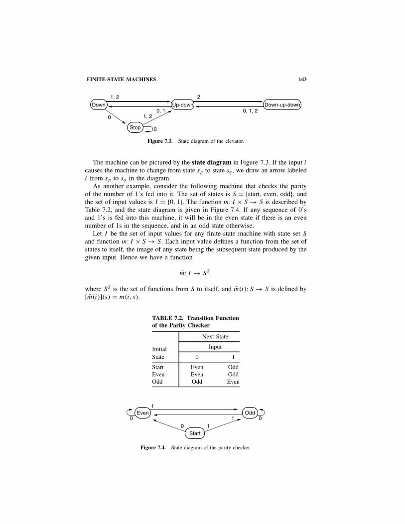
FINITE-STATE MACHINES 143
Up-downDown
Stop
Down-up-down
1, 2
0, 11, 20
0
2
0, 1, 2
Figure 7.3. State diagram of the elevator.
The machine can be pictured by the state diagram in Figure 7.3. If the input i
causes the machine to change from state sp to state sq , we draw an arrow labeledi from sp to sq in the diagram.
As another example, consider the following machine that checks the parityof the number of 1’s fed into it. The set of states is S = {start, even, odd}, andthe set of input values is I = {0, 1}. The function m: I × S → S is described byTable 7.2, and the state diagram is given in Figure 7.4. If any sequence of 0’sand 1’s is fed into this machine, it will be in the even state if there is an evennumber of 1s in the sequence, and in an odd state otherwise.
Let I be the set of input values for any finite-state machine with state set S
and function m: I × S → S. Each input value defines a function from the set ofstates to itself, the image of any state being the subsequent state produced by thegiven input. Hence we have a function
m: I → SS,
where SS is the set of functions from S to itself, and m(i): S → S is defined by[m(i)](s) = m(i, s).
TABLE 7.2. Transition Functionof the Parity Checker
Next State
Initial Input
State 0 1
Start Even OddEven Even OddOdd Odd Even
00 1
1
1
0
Even Odd
Start
Figure 7.4. State diagram of the parity checker.
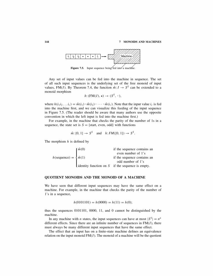
144 7 MONOIDS AND MACHINES
i1 i2 i3 ir• • • Machine
Figure 7.5. Input sequence being fed into a machine.
Any set of input values can be fed into the machine in sequence. The setof all such input sequences is the underlying set of the free monoid of inputvalues, FM(I ). By Theorem 7.4, the function m: I → SS can be extended to amonoid morphism
h: (FM(I ), �) → (SS, Ž ),
where h(i1i2 . . . ir ) = m(i1) Ž m(i2) Ž · · · Ž m(ir ). Note that the input value ir is fedinto the machine first, and we can visualize this feeding of the input sequencein Figure 7.5. (The reader should be aware that many authors use the oppositeconvention in which the left input is fed into the machine first.)
For example, in the machine that checks the parity of the number of 1s in asequence, the state set is S = {start, even, odd} with functions
m: {0, 1} → SS and h: FM({0, 1}) → SS.
The morphism h is defined by
h(sequence) =
m(0) if the sequence contains aneven number of 1’s
m(1) if the sequence contains anodd number of 1’s
identity function on S if the sequence is empty.
QUOTIENT MONOIDS AND THE MONOID OF A MACHINE
We have seen that different input sequences may have the same effect on amachine. For example, in the machine that checks the parity of the number of1’s in a sequence,
h(0101101) = h(0000) = h(11) = h(0);
thus the sequences 0101101, 0000, 11, and 0 cannot be distinguished by themachine.
In any machine with n states, the input sequences can have at most |SS | = nn
different effects. Since there are an infinite number of sequences in FM(I ), theremust always be many different input sequences that have the same effect.
The effect that an input has on a finite-state machine defines an equivalencerelation on the input monoid FM(I ). The monoid of a machine will be the quotient

QUOTIENT MONOIDS AND THE MONOID OF A MACHINE 145
monoid of FM(I ) by this relation. It will always be a finite monoid with, at most,nn elements. We first define the notion of a quotient monoid.
Suppose that R is an equivalence relation on a monoid (M, �). Then R iscalled a congruence relation on M if aRb implies that (a � c)R(b � c) and(c � a)R(c � b) for all c ∈ M . The congruence class containing the elementa ∈ M is the set
[a] = {x ∈ M|xRa}.
Proposition 7.5. If R is a congruence relation on the monoid (M, �), the quotientset M/R = {[a]|a ∈ M} is a monoid under the operation defined by
[a] � [b] = [a � b].
This monoid is called the quotient monoid of M by R.
Proof. We first have to verify that the operation is well defined on congruenceclasses. Suppose that [a] = [a′] and [b] = [b′] so that aRa′ and bRb′. Then(a � b)R(a � b′) and (a � b′)R(a′ � b′). Since R is transitive, (a � b)R(a′ � b′) so[a � b] = [a′ � b′]. This shows that � is well defined on M/R. The associativityof � in M/R follows from the associativity of � in M . If e is the identity of M ,then [e] is the identity of M/R. Hence (M/R, �) is a monoid. �
Let (S, I,m) be a finite-state machine and let the effect of an input sequencebe given by
h: FM(I ) → SS.
Define the relation R on FM(I ) by
αRβ if and only if h(α) = h(β).
This is easily verified to be an equivalence relation. Furthermore, it is a congru-ence relation on the free monoid (FM(I ), �), because if αRβ, then h(α) = h(β),and h(α � γ ) = h(α) Ž h(γ ) = h(β) Ž h(γ ) = h(β � γ ); thus (α � γ )R(β � γ ), andsimilarly, (γ � α)R(γ � β).
The quotient monoid (FM(I )/R, �) is called the monoid of the machine(S, I,m).
We can apply the same construction to the free semigroup of input sequencesto obtain the semigroup of the machine.
The monoid of a machine reflects the capability of the machine to respondto the input sequences. There are an infinite number of sequences in FM(I ),whereas the number of elements in the quotient monoid is less than or equal tonn. Two sequences are in the same congruence class if and only if they have thesame effect on the machine.
A morphism theorem for monoids can be proved in a similar way to themorphism theorem for groups (Theorem 4.25; see Exercise 7.24). Applying this

146 7 MONOIDS AND MACHINES
to the monoid morphism h: FM(I ) → SS , it follows that the quotient monoidFM(I )/R is isomorphic to Im h. This isomorphism assigns to each congruenceclass a unique transition between states.
Example 7.6. Draw the state diagram and find the monoid of the followingmachine (S, I,m). The machine has two states, s0 and s1, and two input sym-bols, 0 and 1. The effects of the input symbols are given by the functionsh(0), h(1): S → S, defined in Table 7.3.
Solution. Let us calculate the effect of inputs of length 2. We have h(ij) =h(i) Ž h(j), where j is fed into the machine first. It follows from Tables 7.3and 7.4 that h(00) = h(01) = h(0) and [00] = [01] = [0] in the monoid of themachine. There are only four functions from {s0, s1} to {s0, s1}, and these areh(0), h(1), h(10), and h(11). Hence the monoid of the machine consists of thefour congruence classes [0], [1], [10], and [11]. The table of this quotient monoidis given in Table 7.5, and the state diagram is given in Figure 7.6. For example,
TABLE 7.3
Initial Next State
State h(0) h(1)
s0 s0 s1
s1 s0 s0
TABLE 7.4
Initial End State
State h(00) h(01) h(10) h(11)
s0 s0 s0 s1 s0
s1 s0 s0 s1 s1
TABLE 7.5. Monoid of the Machine
� [0] [1] [10] [11]
[0] [0] [0] [0] [0][1] [10] [11] [0] [1]
[10] [10] [10] [10] [10][11] [0] [1] [10] [11]
0, 1s1s0
1
0
Figure 7.6. State diagram.

QUOTIENT MONOIDS AND THE MONOID OF A MACHINE 147
[1] � [10] = [110]. Since h(110)(s0) = s0 and h(110)(s1) = s0, it follows that[110] = [0]. Notice that [11] is the identity; thus, in the monoid of the machine,[�] = [11]. �
Example 7.7. Describe the monoid of the machine ({start, even, odd}, {0, 1}, m)
that determines the parity of the number of 1’s in the input.
Solution. We have already seen that any input sequence with an even numberof 1’s has the same effect as 0 and that any sequence with an odd number of1’s has the same effect as 1. It follows from Table 7.6 that the monoid of themachine contains the three elements [�], [0], and [1]. The table for this monoidis given in Table 7.7. �
Finite-state machines can easily be designed to recognize certain types of inputsequences. For example, most numbers inside a computer are in binary form andhave a check digit attached to them so that there is always an even number of1’s in each sequence. This is used to detect any machine errors (see Chapter 14).A finite-state machine like Example 7.7 can be used to perform a parity checkon all the sequences of numbers in the computer. The machine can be designedto signal a parity check error whenever it ends in the “odd” state.
Let us now look at a machine that will recognize the pattern 010 in any binaryinput sequence that is fed into the machine. Figure 7.7 is the state diagram ofsuch a machine. If the machine is initiated in state s1, it will be in state s4 if andonly if the preceding inputs were 010, and in this case, the machine sends anoutput signal.
This machine has four states; thus the total possible number of different func-tions between states is 44 = 256. Table 7.8 shows that the input sequences oflength 0, 1, and 2 all have different effects on the various states. However, sevenof the eight sequences of length 3 have the same effect as sequences of length
TABLE 7.6
Initial Next State
State h(�) h(0) h(1)
Start Start Even OddEven Even Even OddOdd Odd Odd Even
TABLE 7.7. Monoid of the Parity Checker Machine
� [�] [0] [1]
[�] [�] [0] [1][0] [0] [0] [1][1] [1] [1] [0]
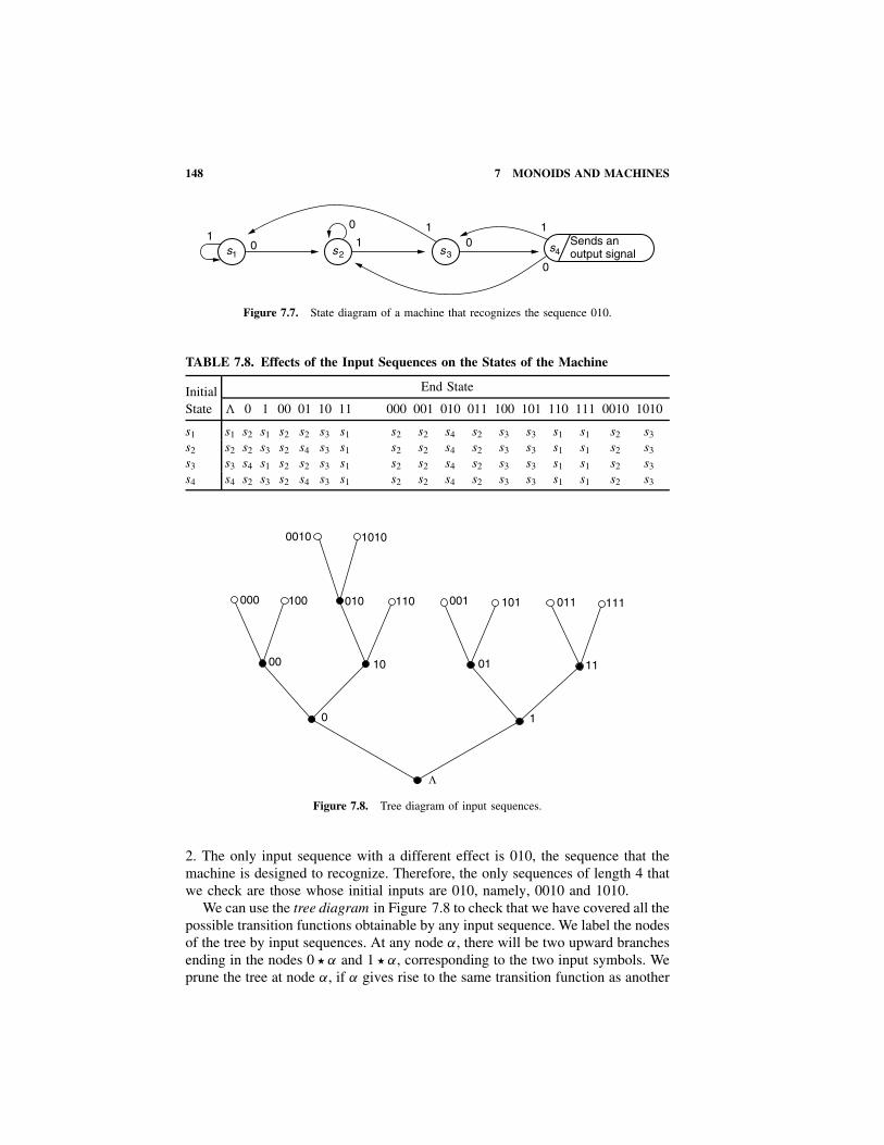
148 7 MONOIDS AND MACHINES
Sends anoutput signals4
0
0
0
01
s1 s2 s31
1 1
Figure 7.7. State diagram of a machine that recognizes the sequence 010.
TABLE 7.8. Effects of the Input Sequences on the States of the Machine
Initial End State
State � 0 1 00 01 10 11 000 001 010 011 100 101 110 111 0010 1010
s1 s1 s2 s1 s2 s2 s3 s1 s2 s2 s4 s2 s3 s3 s1 s1 s2 s3
s2 s2 s2 s3 s2 s4 s3 s1 s2 s2 s4 s2 s3 s3 s1 s1 s2 s3
s3 s3 s4 s1 s2 s2 s3 s1 s2 s2 s4 s2 s3 s3 s1 s1 s2 s3
s4 s4 s2 s3 s2 s4 s3 s1 s2 s2 s4 s2 s3 s3 s1 s1 s2 s3
00
0
10
110000 100 010 001 101 011 111
11
1
0010 1010
01
Λ
Figure 7.8. Tree diagram of input sequences.
2. The only input sequence with a different effect is 010, the sequence that themachine is designed to recognize. Therefore, the only sequences of length 4 thatwe check are those whose initial inputs are 010, namely, 0010 and 1010.
We can use the tree diagram in Figure 7.8 to check that we have covered all thepossible transition functions obtainable by any input sequence. We label the nodesof the tree by input sequences. At any node α, there will be two upward branchesending in the nodes 0 � α and 1 � α, corresponding to the two input symbols. Weprune the tree at node α, if α gives rise to the same transition function as another

EXERCISES 149
TABLE 7.9. Monoid of the Machine That Recognizes 010
� [�] [0] [1] [00] [01] [10] [11] [010]
[�] [�] [0] [1] [00] [01] [10] [11] [010][0] [0] [00] [01] [00] [00] [010] [00] [00][1] [1] [10] [11] [10] [10] [11] [11] [10]
[00] [00] [00] [00] [00] [00] [00] [00] [00][01] [01] [010] [00] [010] [010] [00] [00] [010][10] [10] [10] [10] [10] [10] [10] [10] [10][11] [11] [11] [11] [11] [11] [11] [11] [11]
[010] [010] [010] [010] [010] [010] [010] [010] [010]
node β in the tree. The tree must eventually stop growing because there are onlya finite number of transition functions. Every input sequence has the same effectas one of the solid black nodes in Figure 7.8. These nodes provide a completeset of representatives for the monoid of the machine.
Therefore, the monoid of the machine that recognizes the sequence 010 con-tains only eight elements: [�], [0], [1], [00], [01], [10], [11], and [010], out of apossible 256 transition functions between states. Its table is given in Table 7.9.
For further reading on the mathematical structure of finite-state machines andautomata see Hopcroft et al. [18], Kolman [20], or Stone [22].
EXERCISES
Are the structures described in Exercises 7.1 to 7.13 semigroups or monoids orneither? Give the identity of each monoid.
7.1. (N, gcd).
7.2. (Z, [), where a[b = a.
7.3. (R, �), where x � y = √x2 + y2.
7.4. (R, �), where x � y = 3√
x3 + y3.
7.5. (Z3,−).
7.6. (R, | |), where | | is the absolute value.
7.7. (Z, max), where max (m, n) is the larger of m and n.
7.8. (Z, �), where x � y = x + y + xy.
7.9. (S, gcd), where S = {1, 2, 3, 4, 5, 6}.7.10. (X, max), where X is the set of real-valued functions on the unit interval
[0,1] and if f, g ∈ X, then max (f, g) is the function on X defined by
max(f, g)(x) = max(f (x), g(x)).
7.11. (T , lcm) where T = {1, 2, 4, 5, 10, 20}.
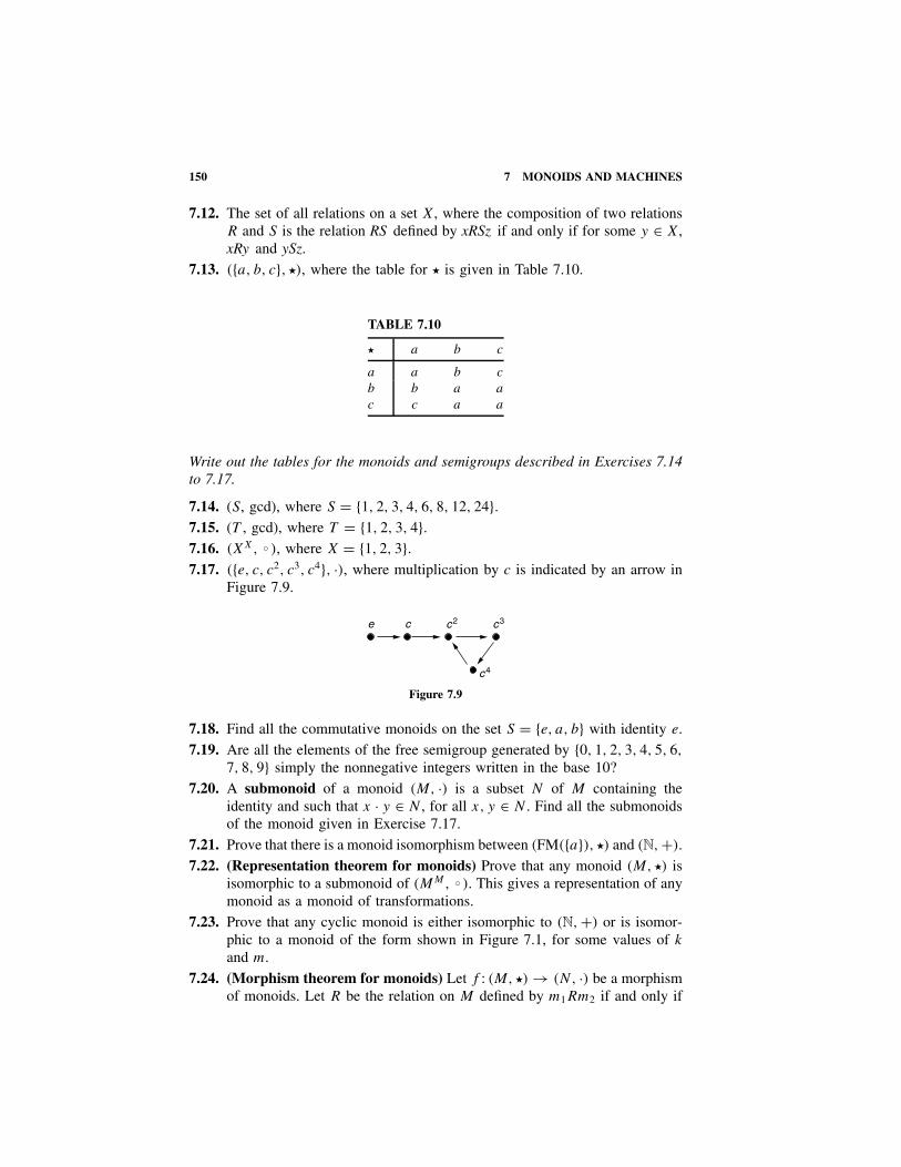
150 7 MONOIDS AND MACHINES
7.12. The set of all relations on a set X, where the composition of two relationsR and S is the relation RS defined by xRSz if and only if for some y ∈ X,xRy and ySz.
7.13. ({a, b, c}, �), where the table for � is given in Table 7.10.
TABLE 7.10
� a b c
a a b c
b b a a
c c a a
Write out the tables for the monoids and semigroups described in Exercises 7.14to 7.17.
7.14. (S, gcd), where S = {1, 2, 3, 4, 6, 8, 12, 24}.7.15. (T , gcd), where T = {1, 2, 3, 4}.7.16. (XX, Ž ), where X = {1, 2, 3}.7.17. ({e, c, c2, c3, c4}, ·), where multiplication by c is indicated by an arrow in
Figure 7.9.
c4
c2 c3ce
Figure 7.9
7.18. Find all the commutative monoids on the set S = {e, a, b} with identity e.7.19. Are all the elements of the free semigroup generated by {0, 1, 2, 3, 4, 5, 6,
7, 8, 9} simply the nonnegative integers written in the base 10?7.20. A submonoid of a monoid (M, ·) is a subset N of M containing the
identity and such that x · y ∈ N , for all x, y ∈ N . Find all the submonoidsof the monoid given in Exercise 7.17.
7.21. Prove that there is a monoid isomorphism between (FM({a}), �) and (N, +).7.22. (Representation theorem for monoids) Prove that any monoid (M, �) is
isomorphic to a submonoid of (MM, Ž ). This gives a representation of anymonoid as a monoid of transformations.
7.23. Prove that any cyclic monoid is either isomorphic to (N, +) or is isomor-phic to a monoid of the form shown in Figure 7.1, for some values of k
and m.
7.24. (Morphism theorem for monoids) Let f : (M, �) → (N, ·) be a morphismof monoids. Let R be the relation on M defined by m1Rm2 if and only if

EXERCISES 151
f (m1) = f (m2). Prove that the quotient monoid (M/R, �) is isomorphicto the submonoid (Imf, ·) of (N, ·). (See Exercise 7.20.)
7.25. An automorphism of a monoid M is an isomorphism from M to itself.Prove that the set of all automorphisms of a monoid M forms a groupunder composition.
7.26. A machine has three states, s1, s2, and s3 and two input symbols, α and β.The effect of the input symbols on the states is given by Table 7.11. Drawthe state diagram and find the monoid of this machine.
TABLE 7.11
Initial Next State
State h(α) h(β)
s1 s1 s1
s2 s3 s1
s3 s2 s1
7.27. Prove that every finite monoid is the monoid of some finite-state machine.
For Exercises 7.28 to 7.30, draw state diagrams of machines with the given inputset, I, that will recognize the given sequence.
7.28. 1101, where I = {0, 1}. 7.29. 0101, where I = {0, 1}.7.30. 2131, where I = {1, 2, 3}.Which of the relations described in Exercises 7.31 to 7.34 are congruence rela-tions on the monoid (N, +)? Find the quotient monoid when the relation is acongruence relation.
7.31. aRb if a − b is even. 7.32. aRb if a > b.7.33. aRb if a = 2rb for some r ∈ Z. 7.34. aRb if 10|(a − b).
The machines in Tables 7.12, 7.13, and 7.14 have state set S = {s1 , s2 , s3 } andinput set I = {0 , 1 }.7.35. Draw the table of the monoid of the machine defined by Table 7.12.
TABLE 7.12
Initial Next State
State h(0) h(1)
s1 s2 s1
s2 s1 s2
s3 s3 s2

152 7 MONOIDS AND MACHINES
7.36. Draw the table of the monoid of the machine defined by Table 7.13.
TABLE 7.13
Initial Next State
State h(0) h(1)
s1 s2 s1
s2 s3 s1
s3 s3 s2
7.37. Find the number of elements in the monoid of the machine defined byTable 7.14.
TABLE 7.14
Initial Next State
State h(0) h(1)
s1 s2 s1
s2 s3 s3
s3 s1 s1
7.38. Find the number of elements in the semigroup of the machine, given byFigure 7.3, that controls the elevator.
7.39. Find the monoid of the machine in Figure 7.10.
s1 s2
s3
a, b
a, b
b
gg
g
a
Figure 7.10
7.40. A serial adder, illustrated in Figure 7.11, is a machine that adds twonumbers in binary form. The two numbers are fed in together, one digitat a time, starting from the right end. Their sum appears as the output.The machine has input symbols 00, 01, 10, and 11, corresponding to therightmost digits of the numbers. Figure 7.12 gives the state diagram ofsuch a machine, where the symbol “sij /j” indicates that the machine is instate sij and emits an output j . The carry digit is the number i of the statesij . Find the monoid of this machine.

EXERCISES 153
Serialadder
Figure 7.11
s00 0
0s10
s01
s11
1
111
11
0010, 01
10, 01
00 00 10, 01
11
1100
10, 01
Figure 7.12. State diagram of the serial adder.
The circuits in Exercises 7.41 to 7.44 represent the internal structures of somefinite-state machines constructed from transistor circuits. These circuits are con-trolled by a clock, and the rectangular boxes denote delays of one time unit. Theinput symbols are 0 and 1 and are fed in at unit time intervals. The internalstates of the machines are described by the contents of the delays. Draw the statediagram and find the elements in the semigroup of each machine.
7.41.Delay
yAND
7.42.
Delayy2
Delayy1
OR
NAND
7.43.Delay
y1
Delayy2
AND
7.44.Delay
y2
Delayy1
NOR

154 7 MONOIDS AND MACHINES
7.45. In the spring, a plant bud has to have the right conditions in order todevelop. One particular bud has to have a rainy day followed by twowarm days, without being interrupted by cool or freezing days, in order todevelop. Furthermore, if a freezing day occurs after the bud has developed,the bud dies. Draw a state diagram for such a bud using the input symbolsR, W , C, F to stand for rainy, warm, cool, and freezing days, respectively.What is the number of elements in the resulting monoid of this bud?
7.46. A dog can either be passive, angry, frightened, or angry and frightened,in which case he bites. If you give him a bone, he becomes passive. Ifyou remove one of his bones, he becomes angry, and, if he is alreadyfrightened, he will bite you. If you threaten him, he becomes frightened,but, if he is already angry, he will bite. Write out the table of the monoidof the dog.

8RINGS AND FIELDS
The familiar number systems of the real or complex numbers contain two basicbinary operations, addition and multiplication. Group theory is not sufficient tocapture all of the algebraic structure of these number systems, because a groupdeals with only one binary operation. It is possible to consider the integers as agroup (Z, +) and the nonzero integers as a monoid (Z∗, ·), but this still neglectsthe relation between addition and multiplication, namely, the fact that multiplica-tion is distributive over addition. We therefore consider algebraic structures withtwo binary operations modeled after these number systems. A ring is a structurethat has the minimal properties we would expect of addition and multiplication.A field is a more specialized ring in which division by nonzero elements isalways possible.
In this chapter we look at the basic properties of rings and fields and con-sider many examples. In later chapters we construct new number systems withproperties similar to the familiar systems.
RINGS
A ring (R, +, ·) is a set R, together with two binary operations + and · on R
satisfying the following axioms. For any elements a, b, c ∈ R,
(i) (a + b) + c = a + (b + c). (associativity of addition)(ii) a + b = b + a. (commutativity of addition)
(iii) there exists 0 ∈ R, called thezero, such that a + 0 = a.
(existence of an additive identity)
(iv) there exists (−a) ∈ R such thata + (−a) = 0.
(existence of an additive inverse)
(v) (a · b) · c = a · (b · c). (associativity of multiplication)(vi) there exists 1 ∈ R such that
1 · a = a · 1 = a.(existence of multiplicative identity)
Modern Algebra with Applications, Second Edition, by William J. Gilbert and W. Keith NicholsonISBN 0-471-41451-4 Copyright 2004 John Wiley & Sons, Inc.
155

156 8 RINGS AND FIELDS
(vii) a · (b + c) = a · b + a · c and(b + c) · a = b · a + c · a.
(distributivity)
Axioms (i)–(iv) are equivalent to saying that (R, +) is an abelian group, andaxioms (v) and (vi) are equivalent to saying that (R, ·) is a monoid.
The ring (R, +, ·) is called a commutative ring if, in addition,
(viii) a · b = b · a for all a, b ∈ R. (commutativity of multiplication)
The integers under addition and multiplication satisfy all of the axioms above,so that (Z, +, ·) is a commutative ring. Also, (Q,+, ·), (R, +, ·), and (C,+, ·)are all commutative rings. If there is no confusion about the operations, we writeonly R for the ring (R, +, ·). Therefore, the rings above would be referred to asZ, Q, R, or C. Moreover, if we refer to a ring R without explicitly defining itsoperations, it can be assumed that they are addition and multiplication.
Many authors do not require a ring to have a multiplicative identity, andmost of the results we prove can be verified to hold for these objects as well.Exercise 8.49 shows that such an object can always be embedded in a ring thatdoes have a multiplicative identity.
The set of all n × n square matrices with real coefficients forms a ring(Mn(R), +, ·), which is not commutative if n > 1, because matrix multiplicationis not commutative.
The elements “even” and “odd” form a commutative ring ({even, odd}, +, ·)where the operations are given by Table 8.1. “Even” is the zero of this ring, and“odd” is the multiplicative identity. This is really a special case of the followingexample when n = 2.
Example 8.1. Show that (Zn, +, ·) is a commutative ring, where addition andmultiplication on congruence classes, modulo n, are defined by the equations[x] + [y] = [x + y] and [x] · [y] = [xy].
Solution. It follows from Example 4.19, that (Zn, +) is an abelian group.Since multiplication on congruence classes is defined in terms of represen-
tatives, it must be verified that it is well defined. Suppose that [x] = [x ′] and[y] = [y ′], so that x ≡ x ′ and y ≡ y ′ mod n. This implies that x = x ′ + kn
and y = y ′ + ln for some k, l ∈ Z. Now x · y = (x ′ + kn) · (y ′ + ln) = x ′ · y ′ +(ky ′ + lx ′ + kln)n, so x · y ≡ x ′ · y ′ mod n and hence [x · y] = [x ′ · y ′]. Thisshows that multiplication is well defined.
TABLE 8.1. Ring of Odd and Even Integers
+ Even Odd
Even even oddOdd odd even
· Even Odd
Even even evenOdd even odd

RINGS 157
The remaining axioms now follow from the definitions of addition and mul-tiplication and from the properties of the integers. The zero is [0], and the unitis [1]. The left distributive law is true, for example, because
[x] · ([y] + [z]) = [x] · [y + z] = [x · (y + z)]
= [x · y + x · z] by distributivity in Z
= [x · y] + [x · z] = [x] · [y] + [x] · [z]. �
Example 8.2. Construct the addition and multiplication tables for the ring(Z5, +, ·).
Solution. We denote the congruence class [x] just by x. The tables are givenin Table 8.2. �
Example 8.3. Show that (Q(√
2), +, ·) is a commutative ring where Q(√
2) ={a + b
√2 ∈ R|a, b ∈ Q}.
Solution. The set Q(√
2) is a subset of R, and the addition and multiplicationis the same as that of real numbers. First, we check that + and · are binaryoperations on Q(
√2). If a, b, c, d ∈ Q, we have
(a + b√
2) + (c + d√
2) = (a + c) + (b + d)√
2 ∈ Q(√
2)
since (a + c) and (b + d) ∈ Q. Also,
(a + b√
2) · (c + d√
2) = (ac + 2bd) + (ad + bc)√
2 ∈ Q(√
2)
since (ac + 2bd) and (ad + bc) ∈ Q.We now check that axioms (i)–(viii) of a commutative ring are valid in Q(
√2).
(i) Addition of real numbers is associative.(ii) Addition of real numbers is commutative.
(iii) The zero is 0 = 0 + 0√
2 ∈ Q(√
2).(iv) The additive inverse of a + b
√2 is (−a) + (−b)
√2 ∈ Q(
√2), since
(−a) and (−b) ∈ Q.
TABLE 8.2. Ring (Z5, +, ·)+ 0 1 2 3 4
0 0 1 2 3 41 1 2 3 4 02 2 3 4 0 13 3 4 0 1 24 4 0 1 2 3
· 0 1 2 3 4
0 0 0 0 0 01 0 1 2 3 42 0 2 4 1 33 0 3 1 4 24 0 4 3 2 1

158 8 RINGS AND FIELDS
(v) Multiplication of real numbers is associative.(vi) The multiplicative identity is 1 = 1 + 0
√2 ∈ Q(
√2).
(vii) The distributive axioms hold for real numbers and hence hold for ele-ments of Q(
√2).
(viii) Multiplication of real numbers is commutative. �
We have already investigated one algebraic system with two binary operations:a boolean algebra. The boolean algebra of subsets of a set is not a ring underthe operations of union and intersection, because neither of these operations hasinverses. However, the symmetric difference does have an inverse, and we canmake a boolean algebra into a ring using this operation and the operation ofintersection.
Example 8.4. (P (X), �,∩) is a commutative ring for any set X.
Solution. The axioms (i)–(viii) of a commutative ring follow from Proposi-tions 2.1 and 2.3. The zero is Ø, and the identity is X. �
In the ring above, A ∩ A = A for every element A in the ring. Such ringsare called boolean rings, since they are all derivable from boolean algebras (seeExercise 8.13).
Example 8.5. Construct the tables for the ring (P (X), �, ∩), where X ={a, b, c}.
Solution. Let A = {a}, B = {b}, and C = {c}, so that A = {b, c}, B = {a, c},and C = {a, b}. Therefore, P (X) = {Ø, A, B,C, A, B, C, X}. The tables for thesymmetric difference and intersection are given in Table 8.3. �
The following properties are useful in manipulating elements of any ring.
Proposition 8.6. If (R, +, ·) is a ring, then for all a, b ∈ R:
(i) a · 0 = 0 · a = 0.(ii) a · (−b) = (−a) · b = −(a · b).
(iii) (−a) · (−b) = a · b.(iv) (−1) · a = −a.(v) (−1) · (−1) = 1.
Proof. (i) By distributivity, a · 0 = a · (0 + 0) = a · 0 + a · 0. Adding−(a · 0) to each side, we obtain 0 = a · 0. Similarly, 0 · a = 0.
(ii) Compute a · (−b) + a · b = a · (−b + b) = a · 0 = 0, using (i). Therefore,a · (−b) = −(a · b). Similarly, (−a) · b = −(a · b).
(iii) We have (−a) · (−b) = −(a · (−b)) = −(−(a · b)) = a · b by (ii) andProposition 3.7.

INTEGRAL DOMAINS AND FIELDS 159
TABLE 8.3. Ring P ({a , b, c})� Ø A B C A B C X
Ø Ø A B C A B C X
A A Ø C B X C B A
B B C Ø A C X A B
C C B A Ø B A X C
A A X C B Ø C B A
B B C X A C Ø A B
C C B A X B A Ø C
X X A B C A B C Ø
∩ Ø A B C A B C X
Ø Ø Ø Ø Ø Ø Ø Ø ØA Ø A Ø Ø Ø A A A
B Ø Ø B Ø B Ø B B
C Ø Ø Ø C C C Ø C
A Ø Ø B C A C B A
B Ø A Ø C C B A B
C Ø A B Ø B A C C
X Ø A B C A B C X
(iv) By (ii), (−1) · a = −(1 · a) = −a.(v) By (iii), (−1) · (−1) = 1 · 1 = 1. �
Proposition 8.7. If 0 = 1, the ring contains only one element and is called thetrivial ring. All other rings are called nontrivial.
Proof. For any element, a, in a ring in which 0 = 1, we have a = a · 1 =a · 0 = 0. Therefore, the ring contains only the element 0. It can be verified thatthis forms a ring with the operations defined by 0 + 0 = 0 and 0 · 0 = 0. �
INTEGRAL DOMAINS AND FIELDS
One very useful property of the familiar number systems is the fact that if ab = 0,then either a = 0 or b = 0. This property allows us to cancel nonzero elementsbecause if ab = ac and a �= 0, then a(b − c) = 0, so b = c. However, this prop-erty does not hold for all rings. For example, in Z4, we have [2] · [2] = [0], andwe cannot always cancel since [2] · [1] = [2] · [3], but [1] �= [3].
If (R, +, ·) is a commutative ring, a nonzero element a ∈ R is called a zerodivisor if there exists a nonzero element b ∈ R such that a · b = 0. A nontrivialcommutative ring is called an integral domain if it has no zero divisors. Hence

160 8 RINGS AND FIELDS
a nontrivial commutative ring is an integral domain if a · b = 0 always impliesthat a = 0 or b = 0.
As the name implies, the integers form an integral domain. Also, Q, R, and C
are integral domains. However, Z4 is not, because [2] is a zero divisor. Neitheris (P (X), �,∩), because every nonempty proper subset of X is a zero divisor.
Mn(R) is not an integral domain (for example,
(0 10 0
)2
= 0).
Proposition 8.8. If a is a nonzero element of an integral domain R anda · b = a · c, then b = c.
Proof. If a · b = a · c, then a · (b − c) = a · b − a · c = 0. Since R is an inte-gral domain, it has no zero divisors. Since a �= 0, it follows that (b − c) = 0.Hence b = c. �
Generally speaking, it is possible to add, subtract, and multiply elements in aring, but it is not always possible to divide. Even in an integral domain, whereelements can be canceled, it is not always possible to divide by nonzero elements.For example, if x, y ∈ Z, then 2x = 2y implies that x = y, but not all elementsin Z can be divided by 2.
The most useful number systems are those in which we can divide by nonzeroelements. A field is a ring in which the nonzero elements form an abelian groupunder multiplication. In other words, a field is a nontrivial commutative ring R
satisfying the following extra axiom.
(ix) For each nonzero element a ∈ R there exists a−1 ∈ R such that a · a−1 = 1.
The rings Q, R, and C are all fields, but the integers do not form a field.
Proposition 8.9. Every field is an integral domain; that is, it has no zero divisors.
Proof. Let a · b = 0 in a field F . If a �= 0, there exists an inverse a−1 ∈ F
and b = (a−1 · a) · b = a−1(a · b) = a−1 · 0 = 0. Hence either a = 0 or b = 0,and F is an integral domain. �
Theorem 8.10. A finite integral domain is a field.
Proof. Let D = {x0, x1, x2, . . . , xn} be a finite integral domain with x0 as 0and x1 as 1. We have to show that every nonzero element of D has a multiplica-tive inverse.
If xi is nonzero, we show that the set xiD = {xix0, xix1, xix2, . . . , xixn} is thesame as the set D. If xixj = xixk, then, by the cancellation property, xj = xk. Henceall the elements xix0, xix1, xix2, . . . , xixn are distinct, and xiD is a subset of D withthe same number of elements. Therefore, xiD = D. But then there is some element,xj , such that xixj = x1 = 1. Hence xj = x−1
i , and D is a field. �

SUBRINGS AND MORPHISMS OF RINGS 161
Note that Z is an infinite integral domain that is not a field.
Theorem 8.11. Zn is a field if and only if n is prime.
Proof. Suppose that n is prime and that [a] · [b] = [0] in Zn. Then n|ab. Son|a or n|b by Euclid’s Lemma (Theorem 12, Appendix 2). Hence [a] = [0] or[b] = [0], and Zn is an integral domain. Since Zn is also finite, it follows fromTheorem 8.10 that Zn is a field.
Suppose that n is not prime. Then we can write n = rs, where r and s areintegers such that 1 < r < n and 1 < s < n. Now [r] �= [0] and [s] �= [0] but[r] · [s] = [rs] = [0]. Therefore, Zn has zero divisors and hence is not a field.
�
Example 8.12. Is (Q(√
2), +, ·) an integral domain or a field?
Solution. From Example 8.3 we know that Q(√
2) is a commutative ring. Leta + b
√2 be a nonzero element, so that at least one of a and b is not zero. Hence
a − b√
2 �= 0 (because√
2 is not in Q), so we have
1
a + b√
2= a − b
√2
(a + b√
2)(a − b√
2)= a
a2 − 2b2−
(b
a2 − 2b2
) √2.
This is an element of Q(√
2), and so is the inverse of a + b√
2. Hence Q(√
2)
is a field (and an integral domain). �
SUBRINGS AND MORPHISMS OF RINGS
If (R, +, ·) is a ring, a nonempty subset S of R is called a subring of R if forall a, b ∈ S:
(i) a + b ∈ S.(ii) −a ∈ S.
(iii) a · b ∈ S.(iv) 1 ∈ S.
Conditions (i) and (ii) imply that (S, +) is a subgroup of (R, +) and can bereplaced by the condition a − b ∈ S.
Proposition 8.13. If S is a subring of (R, +, ·), then (S, +, ·) is a ring.
Proof. Conditions (i) and (iii) of the definition above guarantee that S is closedunder addition and multiplication. Condition (iv) shows that 1 ∈ S. It followsfrom Proposition 3.8 that (S, +) is a group. (S, +, ·) satisfies the remainingaxioms for a ring because they hold in (R, +, ·). �

162 8 RINGS AND FIELDS
For example, Z, Q, and R are all subrings of C. Let D be the set of n × n
real diagonal matrices. Then D is a subring of the ring of all n × n real matri-ces, Mn(R), because the sum, difference, and product of two diagonal matricesis another diagonal matrix. Note that D is commutative even though Mn(R)
is not.
Example 8.14. Show that Q(√
2) = {a + b√
2|a, b ∈ Q} is a subring of R.
Solution. Let a + b√
2, c + d√
2 ∈ Q(√
2). Then
(i) (a + b√
2) + (c + d√
2) = (a + c) + (b + d)√
2 ∈ Q(√
2).(ii) −(a + b
√2) = (−a) + (−b)
√2 ∈ Q(
√2).
(iii) (a + b√
2) · (c + d√
2) = (ac + 2bd) + (ad + bc)√
2 ∈ Q(√
2).(iv) 1 = 1 + 0
√2 ∈ Q(
√2). �
A morphism between two rings is a function between their underlying setsthat preserves the two operations of addition and multiplication and also theelement 1. Many authors use the term homomorphism instead of morphism.
More precisely, let (R, +, ·) and (S, +, ·) be two rings. The function f : R → S
is called a ring morphism if for all a, b ∈ R:
(i) f (a + b) = f (a) + f (b).
(ii) f (a · b) = f (a) · f (b).(iii) f (1) = 1.
If the operations in the two rings are denoted by different symbols, forexample, if the rings are (R, +, ·) and (S, ⊕,Ž), then the conditions forf : R → S to be a ring morphism are:
(i) f (a + b) = f (a) ⊕ f (b).
(ii) f (a · b) = f (a)Žf (b).(iii) f (1R) = 1S where 1R and 1S are the respective identities.
A ring isomorphism is a bijective ring morphism. If there is an isomorphismbetween the rings R and S, we say R and S are isomorphic rings and writeR ∼= S.
A ring morphism, f , from (R, +, ·) to (S, +, ·) is, in particular, a groupmorphism from (R, +) to (S, +). Therefore, by Proposition 3.19, f (0) = 0 andf (−a) = −f (a) for all a ∈ R.
The inclusion function, i: S → R, of any subring S into a ring R is alwaysa ring morphism. The function f : Z → Zn, defined by f (x) = [x], which mapsan integer to its equivalence class modulo n, is a ring morphism from (Z, +, ·)to (Zn,+, ·).

SUBRINGS AND MORPHISMS OF RINGS 163
Example 8.15. If X is a one element set, show that f : P (X) → Z2 is aring isomorphism between (P (X), �, ∩) and (Z2,+, ·), where f (Ø) = [0] andf (X) = [1].
Solution. We can check that f is a morphism by testing all the possibilitiesfor f (A�B) and f (A ∩ B). Since the rings are commutative, they are
f (Ø�Ø) = f (Ø) = [0] = f (Ø) + f (Ø)
f (Ø�X) = f (X) = [1] = f (Ø) + f (X)
f (X�X) = f (Ø) = [0] = f (X) + f (X)
f (Ø ∩ Ø) = f (Ø) = [0] = f (Ø) · f (Ø)
f (Ø ∩ X) = f (Ø) = [0] = f (Ø) · f (X)
f (X ∩ X) = f (X) = [1] = f (X) · f (X).
Both rings contain only two elements, and f is a bijection; therefore, f is anisomorphism. �
If f : R → S is an isomorphism between two finite rings, the addition andmultiplication tables of S will be the same as those of R if we replace eacha ∈ R by f (a) ∈ S. For example, Tables 8.4 and 8.5 illustrate the isomorphismof Example 8.15.
The following ring isomorphism between linear transformations and matricesis the crux of much of linear algebra.
Example 8.16. The linear transformations from Rn to itself form a ring,(L(Rn, Rn), +, Ž ), under addition and composition. Show that the function
f : L(Rn, Rn) → Mn(R)
TABLE 8.4. Ring P (X )
When X Is a Point
� Ø X
Ø Ø X
X X Ø
∩ Ø X
Ø Ø ØX Ø X
TABLE 8.5. Ring Z2
+ [0] [1]
[0] [0] [1][1] [1] [0]
· [0] [1]
[0] [0] [0][1] [0] [1]

164 8 RINGS AND FIELDS
is a ring morphism, where f assigns to each linear transformation its standardmatrix, that is, its n × n coefficient matrix with respect to the standard basisof Rn.
Solution. If α is a linear transformation from Rn to itself, then
α
x1...
xn
=
a11x1 + · · · + a1nxn
......
an1x1 + · · · + annxn
and f (α) =
a11 . . . a1n
......
an1 . . . ann
.
Matrix addition and multiplication is defined so that f (α + β) = f (α) + f (β)
and f (α Ž β) = f (α) · f (β). Also, if ι is the identity linear transformation thenf (ι) is the identity matrix.
Any matrix defines a linear transformation, so that f is surjective. Fur-thermore, f is injective, because any matrix can arise from only one lineartransformation. In fact, the j th column of the matrix must be the image of thej th basis vector. Hence f is an isomorphism. �
Example 8.17. Show that f : Z24 → Z4, defined by f ([x]24) = [x]4 is a ringmorphism.
Proof. Since the function is defined in terms of representatives of equiva-lence classes, we first check that it is well defined. If [x]24 = [y]24,then x ≡ y mod 24 and 24|(x − y). Hence 4|(x − y) and [x]4 = [y]4, whichshows that f is well defined.
We now check the conditions for f to be a ring morphism.
(i) f ([x]24 + [y]24) = f ([x + y]24) = [x + y]4 = [x]4 + [y]4.(ii) f ([x]24 · [y]24) = f ([xy]24) = [xy]4 = [x]4 · [y]4.
(iii) f ([1]24) = [1]4. �
NEW RINGS FROM OLD
This section introduces various methods for constructing new rings from givenrings. These include the direct product of rings, matrix rings, polynomial rings,rings of sequences, and rings of formal power series. Perhaps the most impor-tant class of rings constructible from given rings is the class of quotient rings.Their construction is analogous to that of quotient groups and is discussed inChapter 10.
If (R, +, ·) and (S, +, ·) are two rings, their product is the ring (R × S, +, ·)whose underlying set is the cartesian product of R and S and whose operationsare defined component-wise by
(r1, s1) + (r2, s2) = (r1 + r2, s1 + s2) and (r1, s1) · (r2, s2) = (r1 · r2, s1 · s2).

NEW RINGS FROM OLD 165
It is readily verified that these operations do indeed define a ring structure onR × S whose zero is (0R, 0S), where 0R and 0S are the zeros of R and S, andwhose multiplicative identity is (1R, 1S), where 1R and 1S are the identities in R
and S.The product construction can be iterated any number of times. For example,
(Rn, +, ·) is a commutative ring, where Rn is the n-fold cartesian product of R
with itself.
Example 8.18. Write down the addition and multiplication tables for Z2 × Z3.
Solution. Let Z2 = {0, 1} and Z3 = {0, 1, 2}. Then Z2 × Z3 = {(0, 0), (0, 1),
(0, 2), (1, 0), (1, 1), (1, 2)}. The addition and multiplication tables are given inTable 8.6. In calculating these, it must be remembered that addition and mul-tiplication are performed modulo 2 in the first coordinate and modulo 3 in thesecond coordinate. �
We know that Z2 × Z3 and Z6 are isomorphic as groups; we now show thatthey are isomorphic as rings.
Theorem 8.19. Zm × Zn is isomorphic as a ring to Zmn if and only ifgcd(m, n) = 1.
Proof. If gcd(m, n) = 1, it follows from Theorems 4.32 and 3.20 that thefunction
f : Zmn → Zm × Zn
TABLE 8.6. Ring Z2 × Z3
+ (0, 0) (0, 1) (0, 2) (1, 0) (1, 1) (1, 2)
(0, 0) (0, 0) (0, 1) (0, 2) (1, 0) (1, 1) (1, 2)(0, 1) (0, 1) (0, 2) (0, 0) (1, 1) (1, 2) (1, 0)(0, 2) (0, 2) (0, 0) (0, 1) (1, 2) (1, 0) (1, 1)(1, 0) (1, 0) (1, 1) (1, 2) (0, 0) (0, 1) (0, 2)(1, 1) (1, 1) (1, 2) (1, 0) (0, 1) (0, 2) (0, 0)(1, 2) (1, 2) (1, 0) (1, 1) (0, 2) (0, 0) (0, 1)
· (0, 0) (0, 1) (0, 2) (1, 0) (1, 1) (1, 2)
(0, 0) (0, 0) (0, 0) (0, 0) (0, 0) (0, 0) (0, 0)(0, 1) (0, 0) (0, 1) (0, 2) (0, 0) (0, 1) (0, 2)(0, 2) (0, 0) (0, 2) (0, 1) (0, 0) (0, 2) (0, 1)(1, 0) (0, 0) (0, 0) (0, 0) (1, 0) (1, 0) (1, 0)(1, 1) (0, 0) (0, 1) (0, 2) (1, 0) (1, 1) (1, 2)(1, 2) (0, 0) (0, 2) (0, 1) (1, 0) (1, 2) (1, 1)

166 8 RINGS AND FIELDS
defined by f ([x]mn) = ([x]m, [x]n) is a group isomorphism. However, this func-tion also preserves multiplication because
f ([x]mn · [y]mn) = f ([xy]mn) = ([xy]m, [xy]n) = ([x]m[y]m, [x]n[y]n)
= ([x]m, [x]n) · ([y]m, [y]n) = f ([x]mn) · f ([y]mn).
Also, f ([1]mn) = ([1]m, [1]n); thus f is a ring isomorphism.It was shown in the discussion following Corollary 4.33 that if gcd(m, n) �=
1, Zm × Zn and Zmn are not isomorphic as groups, and hence they cannot beisomorphic as rings. �
We can extend this result by induction to show the following.
Theorem 8.20. Let m = m1 · m2 · · · mr , where gcd(mi, mj ) = 1 if i �= j . ThenZm1 × Zm2 × · · · × Zmr
is a ring isomorphic to Zm.
Corollary 8.21. Let n = pα11 p
α22 · · ·pαr
r be a decomposition of the integer n intopowers of distinct primes. Then Zn
∼= Zpα11
× Zpα22
× · · · × Zpαrr
as rings.
If R is a commutative ring, we can construct the ring of n × n matrices withentries from R, (Mn(R), +, ·). Addition and multiplication are performed as inreal matrices.
For example, (Mn(Z2), +, ·) is the ring of n × n matrices with 0 and 1 entries.Addition and multiplication is performed modulo 2. This is a noncommutativering with 2(n2) elements.
If R is a commutative ring, a polynomial p(x) in the indeterminate x overthe ring R is an expression of the form
p(x) = a0 + a1x + a2x2 + · · · + anx
n,
where a0, a1, a2, . . . , an ∈ R and n ∈ N. The element ai is called the coefficientof xi in p(x). If the coefficient of xi is zero, the term 0xi may be omitted, andif the coefficient of xi is one, 1xi may be written simply as xi .
Two polynomials f (x) and g(x) are called equal when they are identical, thatis, when the coefficient of xn is the same in each polynomial for every n � 0.In particular,
a0 + a1x + a2x2 + · · · + anx
n = 0
is the zero polynomial if and only if a0 = a1 = a2 = · · · = an = 0.If n is the largest integer for which an �= 0, we say that p(x) has degree n and
write degp(x) = n. If all the coefficients of p(x) are zero, then p(x) is calledthe zero polynomial, and its degree is not defined.
For example, 4x2 − √3 is a polynomial over R of degree 2, ix4 − (2 + i)x3 +
3x is a polynomial over C of degree 4, and x7 + x5 + x4 + 1 is a polynomialover Z2 of degree 7. The number 5 is a polynomial over Z of degree 0; the zero

NEW RINGS FROM OLD 167
polynomial and the polynomials of degree 0 are called constant polynomialsbecause they contain no x terms.
The set of all polynomials in x with coefficients from the commutative ringR is denoted by R[x]. That is,
R[x] = {a0 + a1x + a2x2 + · · · + anx
n|ai ∈ R, n ∈ N}.
This forms a ring (R[x], +, ·) called the polynomial ring with coefficients fromR when addition and multiplication of the polynomials
p(x) =n∑
i=0
aixi and q(x) =
m∑i=0
bixi
are defined by
p(x) + q(x) =max(m,n)∑
i=0
(ai + bi)xi
and
p(x) · q(x) =m+n∑k=0
ckxk where ck =
∑i+j=k
aibj .
With a little effort, it can be verified that (R[x], +, ·) satisfies all the axiomsfor a commutative ring. The zero is the zero polynomial, and the multiplicativeidentity is the constant polynomial 1.
For example, in Z5[x], the polynomial ring with coefficients in the integersmodulo 5, we have
(2x3 + 2x2 + 1) + (3x2 + 4x + 1) = 2x3 + 4x + 2
and(2x3 + 2x2 + 1) · (3x2 + 4x + 1) = x5 + 4x4 + 4x + 1.
When working in Zn[x], the coefficients, but not the exponents, are reducedmodulo n.
Proposition 8.22. If R is an integral domain and p(x) and q(x) are nonzeropolynomials in R[x], then
deg(p(x) · q(x)) = deg p(x) + deg q(x).
Proof. Let deg p(x) = n, deg q(x) = m and let p(x) = a0 + · · · + anxn,
q(x) = b0 + · · · + bmxm, where an �= 0, bm �= 0. Then the coefficient of the high-est power of x in p(x) · q(x) is anbm, which is nonzero since R has no zerodivisors. Hence deg(p(x) · q(x)) = m + n. �
168 8 RINGS AND FIELDS
If the coefficient ring is not an integral domain, the degree of a product may beless than the sum of the degrees. For example, (2x3 + x) · (3x) = 3x2 in Z6[x].
Corollary 8.23. If R is an integral domain, so is R[x].
Proof. If p(x) and q(x) are nonzero elements of R[x], then p(x) · q(x) isalso nonzero by Proposition 8.22. Hence R[x] has no zero divisors. �
The construction of a polynomial ring can be iterated to obtain the ring ofpolynomials in n variables x1, . . . , xn, with coefficients from R. We define induc-tively R[x1, . . . , xn] = R[x1, . . . , xn−1][xn]. For example, consider a polynomialf in R[x, y] = R[x][y], say
f = f0 + f1y + f2y2 + · · · + fny
n,
where each fi = fi(x) is in R[x]. If we write fi = a0i + a1ix + a2ix2 · · · for
each i, then
f (x, y) = a00 + a10x + a01y + a20x2 + a11xy + a02y
2 + · · · .Clearly, we can prove by induction from Corollary 8.22 that R[x1, . . . , xn] is
an integral domain if R is an integral domain.
Proposition 8.24. Let R be a commutative ring and denote the infinite sequenceof elements of R, 〈a0, a1, a2, . . .〉, by 〈ai〉. Define addition, +, and convolution,∗, of two such sequences by
〈ai〉 + 〈bi〉 = 〈ai + bi〉and
〈ai〉 ∗ 〈bi〉 =⟨ ∑
j+k=i
aj bk
⟩= 〈a0bi + a1bi−1 + · · · + aib0〉.
The set of all such sequences forms a commutative ring (RN, +, ∗) called thering of sequences in R. If R is an integral domain, so is RN.
Proof. Addition is clearly associative and commutative. The zero element isthe zero sequence 〈0〉 = 〈0, 0, 0, . . .〉, and the negative of 〈ai〉 is 〈−ai〉. Now
(〈ai〉 ∗ 〈bi〉) ∗ 〈ci〉 =⟨ ∑
j+k=i
aj bk
⟩∗ 〈ci〉
=⟨ ∑
l+m=i
∑
j+k=m
ajbk
cl
⟩=
⟨ ∑j+k+l=i
aj bkcl
⟩.
NEW RINGS FROM OLD 169
Similarly, bracketing the sequences in the other way, we obtain the same result,which shows that convolution is associative.
Convolution is clearly commutative and the distributive laws hold because
〈ai〉 ∗ (〈bi〉 + 〈ci〉) =⟨ ∑
j+k=i
aj (bk + ck)
⟩
=⟨ ∑
j+k=i
ajbk
⟩+
⟨ ∑j+k=i
aj ck
⟩= 〈ai〉 ∗ 〈bi〉 + 〈ai〉 ∗ 〈ci〉.
The identity in the ring of sequences is 〈1, 0, 0, . . .〉 because
〈1, 0, 0, . . .〉 ∗ 〈a0, a1, a2, . . .〉 = 〈1a0, 1a1 + 0a0, 1a2 + 0a1 + 0a0, . . .〉= 〈a0, a1, a2, . . .〉.
Therefore, (RN, +, ∗) is a commutative ring.Suppose that aq and br are the first nonzero elements in the nonzero sequences
〈ai〉 and 〈bi〉, respectively. Then the element in the (q + r)th position of theirconvolution is∑j+k=q+r
aj bk = a0bq+r + a1bq+r−1 + · · · + aqbr + aq+1br−1 + · · · + aq+rb
= 0 + 0 + · · · + aqbr + 0 + · · · + 0 = aqbr .
Hence, if R is an integral domain, this element is not zero and the ring ofsequences has no zero divisors. �
The ring of sequences cannot be a field because 〈0, 1, 0, 0, . . .〉 has no inverse.In fact, for any sequence 〈bi〉, 〈0, 1, 0, 0, . . .〉 ∗ 〈b0, b1, b2, . . .〉 = 〈0, b0, b1, . . .〉,which can never be the identity in the ring.
A formal power series in x with coefficients from a commutative ring R isan expression of the form.
a0 + a1x + a2x2 + · · · =
∞∑i=0
aixi where ai ∈ R.
In contrast to a polynomial, these power series can have an infinite number ofnonzero terms.
We denote the set of all such formal power series by R[[x]]. The term formal isused to indicate that questions of convergence of these series are not considered.Indeed, over many rings, such as Zn, convergence would not be meaningful.
Motivated by RN, addition and multiplication are defined in R[[x]] by( ∞∑
i=0
aixi
)+
( ∞∑i=0
bixi
)=
∞∑i=0
(ai + bi)xi
170 8 RINGS AND FIELDS
and ( ∞∑i=0
aixi
)·( ∞∑
i=0
bixi
)=
∞∑i=0
∑
j+k=i
ajbk
xi .
It can be verified that these formal power series do form a ring, (R[[x]],+, ·),and that the polynomial ring, R[x], is the subring consisting of those powerseries with only a finite number of nonzero terms. In fact, the ring of sequences(RN, +, ∗) is isomorphic to the ring of formal power series (R[[x]],+, ·). Thefunction f : RN → R[[x]] that is defined by f (〈a0, a1, a2, · · ·〉) = a0 + a1x +a2x2 + · · · is clearly a bijection. It follows from the definitions of addition, mul-tiplication, and convolution in these rings, that f is a ring morphism.
FIELD OF FRACTIONS
We can always add, subtract, and multiply elements in any ring, but we cannotalways divide. However, if the ring is an integral domain, it is possible to enlargeit so that division by nonzero elements is possible. In other words, we can con-struct a field containing the given ring as a subring. This is precisely what we didfollowing Example 4.2 when constructing the rational numbers from the integers.
If the original ring did have zero divisors or was noncommutative, it couldnot possibly be a subring of any field, because fields cannot contain zero divisorsor pairs of noncommutative elements.
Theorem 8.25. If R is an integral domain, it is possible to construct a field Q,so that the following hold:
(i) R is isomorphic to a subring, R′, of Q.
(ii) Every element of Q can be written as p · q−1 for suitable p, q ∈ R′.
Q is called the field of fractions of R (or sometimes the field of quotients of R).
Proof. Consider the set R × R∗ = {(a, b)|a, b ∈ R, b �= 0}, consisting of pairsof elements of R, the second being nonzero. Motivated by the fact that a
b= c
d
in Q if and only if ad = bc, we define a relation ∼ on R × R∗ by
(a, b) ∼ (c, d) if and only if ad = bc in R.
We verify that this is an equivalence relation.
(i) (a, b) ∼ (a, b), since ab = ba.
(ii) If (a, b) ∼ (c, d), then ad = bc. This implies that cb = da and hencethat (c, d) ∼ (a, b).

FIELD OF FRACTIONS 171
(iii) If (a, b) ∼ (c, d) and (c, d) ∼ (e, f ), then ad = bc and cf = de. Thisimplies that (af − be)d = (ad)f − b(ed) = bcf − bcf = 0. Since R hasno zero divisors and d �= 0, it follows that af = be and (a, b) ∼ (e, f ).
Hence the relation ∼ is reflexive, symmetric, and transitive.Denote the equivalence class containing (a, b) by a/b and the set of equiva-
lence classes by Q. As in Q, define addition and multiplication in Q by
a
b+ c
d= ad + bc
bdand
a
b· c
d= ac
bd.
These operations on equivalence classes are defined in terms of particular repre-sentatives, so it must be checked that they are well defined. If a/b = a′/b′ andc/d = c′/d ′, then ab′ = a′b and cd ′ = c′d . Hence
(ad + bc)(b′d ′) = (ab′)dd ′ + bb′(cd ′) = (a′b)dd ′ + bb′(c′d)
= (a′d ′ + b′c′)(bd)
and thereforead + bc
bd= a′d ′ + b′c′
b′d ′ , which shows that addition is well defined.
Also, acb′d ′ = a′c′bd; thusac
bd= a′c′
b′d ′ , which shows that multiplication is well
defined.It can now be verified that (Q, +, ·) is a field. The zero is 0/1, and the identity
is 1/1. For example, the distributive laws hold because
a
b·(
c
d+ e
f
)= a
b· cf + de
df= a(cf + de)
bdf= a(cf + de)
bdf· b
b= ac
bd+ ae
bf
= a
b· c
d+ a
b· e
f.
The inverse of any nonzero elementa
bis
b
a. The remaining axioms for a field
are straightforward to check.
The ring R is isomorphic to the subring R′ ={
r
1
∣∣∣∣r ∈ R
}of Q by an iso-
morphism that maps r tor
1. Any element
a
bin the field Q can be written as
a
b= a
1· 1
b= a
1
(b
1
)−1
wherea
1and
b
1are in R′. �
If we take R = Z to be integers in the above construction, we obtain therational numbers Q as the field of fractions.

172 8 RINGS AND FIELDS
If R is an integral domain, the field of fractions of the polynomial ring R[x]is called the field of rational functions with coefficients in R. Its elements canbe considered as fractions of one polynomial over a nonzero polynomial.
A (possibly noncommutative) ring is called a domain if ab = 0 if and onlyif a = 0 or b = 0. Thus the commutative domains are precisely the integraldomains. In 1931, Oystein Ore (1899–1968) extended Theorem 8.25 to a classof domains (now called left Ore domains) for which a ring of left fractionscan be constructed that is a skew field (that is, a field that is not necessarilycommutative). On the other hand, in 1937, A. I. Mal’cev (1909–1967) discov-ered an example of a domain that cannot be embedded in any skew field. Thesimplest example of a noncommutative skew field is the ring of quaternions(see Exercise 8.36). It has infinitely many elements, in agreement with a famoustheorem of J. H. M. Wedderburn, proved in 1905, asserting that any finite skewfield is necessarily commutative.
CONVOLUTION FRACTIONS
We now present an application of the field of fractions that has important implica-tions in analysis. This example is of a different type than most of the applicationsin this book. It can be omitted, without loss of continuity, by those readers notinterested in analysis or applied mathematics.
We construct the field of fractions of a set of continuous functions, and useit to explain two mathematical techniques that have been used successfully byengineers and physicists for many years, but were at first mistrusted by math-ematicians because they did not have a firm mathematical basis. One suchtechnique was introduced by O. Heaviside in 1893 in dealing with electricalcircuits; this is called the operational calculus, and it enabled him to solve par-tial differential equations by manipulating differential operators as if they werealgebraic quantities. The second such technique is the use of impulse functionsin applied mathematics and mathematical physics. In 1926, when solving prob-lems in relativistic quantum mechanics, P. Dirac introduced his delta function,δ(x), which has the property that
δ(x) = 0 if x �= 0 and∫ ∞
−∞δ(x) dx = 1.
If we use the usual definition of functions, no such object exists. However, itcan be pictured in Figure 8.1 as the limit, as k tends to zero, of the functionsδk(x), where
δk(x) ={
1/k if 0 � x � k.
0 otherwise
Each function δk(x) vanishes outside the interval 0 � x � k and has the prop-erty that ∫ ∞
−∞δk(x) dx = 1.

CONVOLUTION FRACTIONS 173
x x
d1 d1/2
x
d1/4
Figure 8.1. The Dirac delta “function” is the limit of δk as k tends to zero.
Consider the set, C[0, ∞), of real-valued functions that are continuous in theinterval 0 � x < ∞. We define the operations of addition and convolution on thisset so that the algebraic structure (C[0, ∞), +, ∗) is nearly an integral domain:convolution does not have an identity so the structure fails to satisfy Axiom(vi) of a ring. However, it is still possible to embed this structure in its fieldof fractions. The Polish mathematician Jan Mikusinski constructed this field offractions and called such elements operators or generalized functions. The Diracdelta function is a generalized function and is in fact the identity for convolutionin the field of fractions.
Define addition and convolution of two functions f and g in C[0, ∞) by
(f + g)(x) = f (x) + g(x) and (f ∗ g)(x) =∫ x
0f (t)g(x − t) dt.
This convolution of functions is the continuous analogue of convolution ofsequences, as can be seen by writing the ith term of the sequence
〈ai〉 ∗ 〈bi〉 asi∑
t=0
atbi−t .
It is clear that addition is associative and commutative, and the zero functionis the additive identity. Also, the negative of f (x) is −f (x).
Convolution is commutative because
(f ∗ g)(x) =∫ x
0f (t)g(x − t) dt
= −∫ 0
x
f (x − u)g(u) du substituting u = x − t
=∫ x
0g(u)f (x − u) du = (g ∗ f )(x).
Convolution is associative because
(f ∗ (g ∗ h))(x) =∫ x
0f (t)(g ∗ h)(x − t) dt
=∫ x
0f (t)
[∫ x−t
0g(u)h(x − t − u) du
]dt
=∫ x
0f (t)
[∫ x
t
g(w − t)h(x − w) dw
]dt,
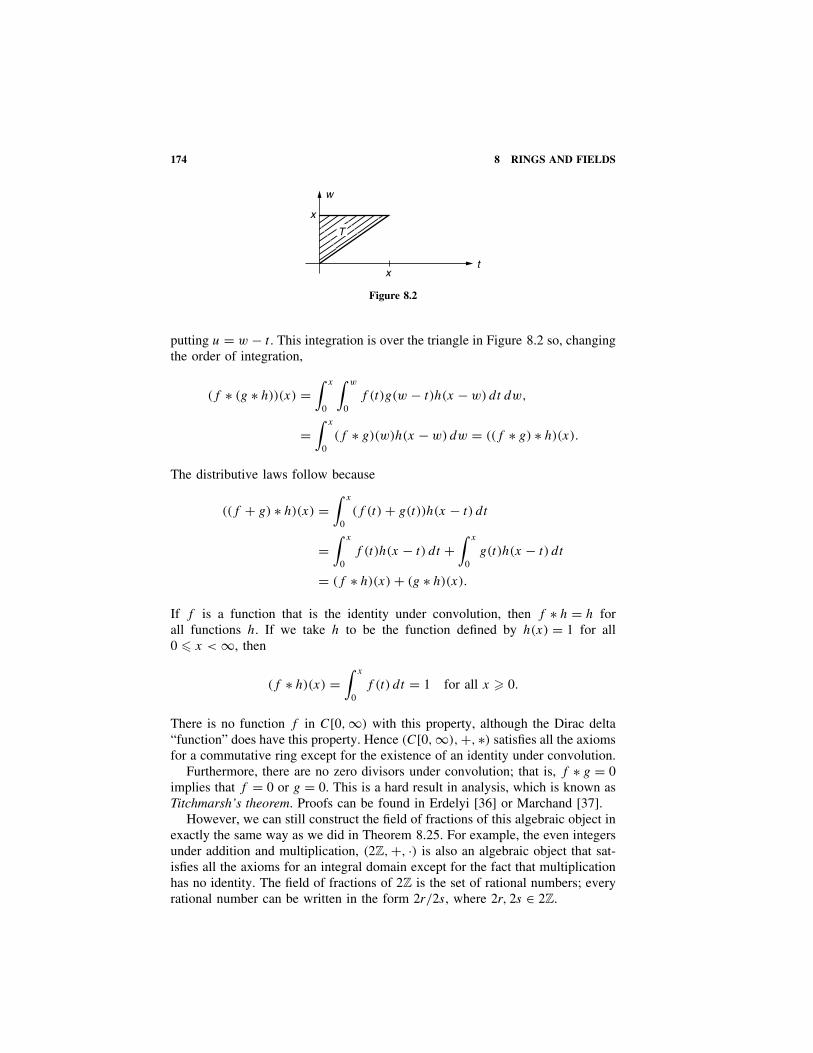
174 8 RINGS AND FIELDS
tx
x
T
w
Figure 8.2
putting u = w − t . This integration is over the triangle in Figure 8.2 so, changingthe order of integration,
(f ∗ (g ∗ h))(x) =∫ x
0
∫ w
0f (t)g(w − t)h(x − w) dt dw,
=∫ x
0(f ∗ g)(w)h(x − w) dw = ((f ∗ g) ∗ h)(x).
The distributive laws follow because
((f + g) ∗ h)(x) =∫ x
0(f (t) + g(t))h(x − t) dt
=∫ x
0f (t)h(x − t) dt +
∫ x
0g(t)h(x − t) dt
= (f ∗ h)(x) + (g ∗ h)(x).
If f is a function that is the identity under convolution, then f ∗ h = h forall functions h. If we take h to be the function defined by h(x) = 1 for all0 � x < ∞, then
(f ∗ h)(x) =∫ x
0f (t) dt = 1 for all x � 0.
There is no function f in C[0, ∞) with this property, although the Dirac delta“function” does have this property. Hence (C[0, ∞), +, ∗) satisfies all the axiomsfor a commutative ring except for the existence of an identity under convolution.
Furthermore, there are no zero divisors under convolution; that is, f ∗ g = 0implies that f = 0 or g = 0. This is a hard result in analysis, which is known asTitchmarsh’s theorem. Proofs can be found in Erdelyi [36] or Marchand [37].
However, we can still construct the field of fractions of this algebraic object inexactly the same way as we did in Theorem 8.25. For example, the even integersunder addition and multiplication, (2Z, +, ·) is also an algebraic object that sat-isfies all the axioms for an integral domain except for the fact that multiplicationhas no identity. The field of fractions of 2Z is the set of rational numbers; everyrational number can be written in the form 2r/2s, where 2r, 2s ∈ 2Z.
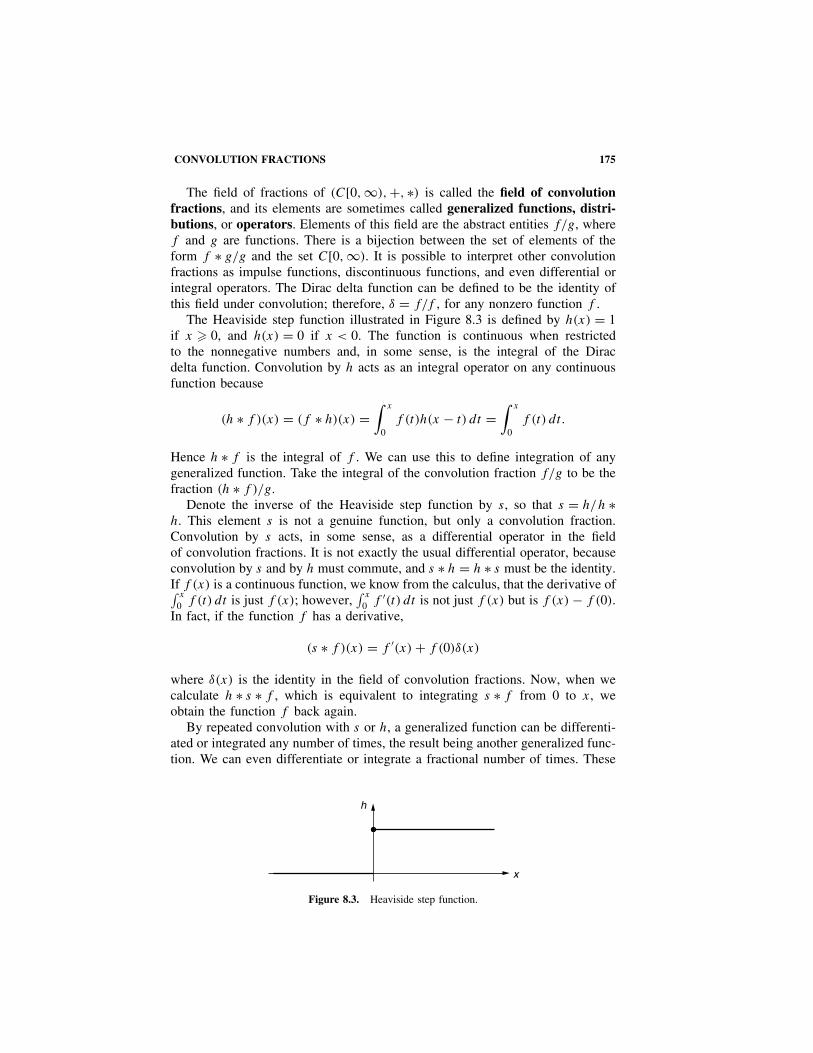
CONVOLUTION FRACTIONS 175
The field of fractions of (C[0, ∞), +, ∗) is called the field of convolutionfractions, and its elements are sometimes called generalized functions, distri-butions, or operators. Elements of this field are the abstract entities f/g, wheref and g are functions. There is a bijection between the set of elements of theform f ∗ g/g and the set C[0, ∞). It is possible to interpret other convolutionfractions as impulse functions, discontinuous functions, and even differential orintegral operators. The Dirac delta function can be defined to be the identity ofthis field under convolution; therefore, δ = f/f , for any nonzero function f .
The Heaviside step function illustrated in Figure 8.3 is defined by h(x) = 1if x � 0, and h(x) = 0 if x < 0. The function is continuous when restrictedto the nonnegative numbers and, in some sense, is the integral of the Diracdelta function. Convolution by h acts as an integral operator on any continuousfunction because
(h ∗ f )(x) = (f ∗ h)(x) =∫ x
0f (t)h(x − t) dt =
∫ x
0f (t) dt.
Hence h ∗ f is the integral of f . We can use this to define integration of anygeneralized function. Take the integral of the convolution fraction f/g to be thefraction (h ∗ f )/g.
Denote the inverse of the Heaviside step function by s, so that s = h/h ∗h. This element s is not a genuine function, but only a convolution fraction.Convolution by s acts, in some sense, as a differential operator in the fieldof convolution fractions. It is not exactly the usual differential operator, becauseconvolution by s and by h must commute, and s ∗ h = h ∗ s must be the identity.If f (x) is a continuous function, we know from the calculus, that the derivative of∫ x
0 f (t) dt is just f (x); however,∫ x
0 f ′(t) dt is not just f (x) but is f (x) − f (0).In fact, if the function f has a derivative,
(s ∗ f )(x) = f ′(x) + f (0)δ(x)
where δ(x) is the identity in the field of convolution fractions. Now, when wecalculate h ∗ s ∗ f , which is equivalent to integrating s ∗ f from 0 to x, weobtain the function f back again.
By repeated convolution with s or h, a generalized function can be differenti-ated or integrated any number of times, the result being another generalized func-tion. We can even differentiate or integrate a fractional number of times. These
h
x
Figure 8.3. Heaviside step function.

176 8 RINGS AND FIELDS
operations s and h can be used to explain Heaviside’s operational calculus, inwhich differential and integral operators are manipulated like algebraic symbols.
For further information on the algebraic aspects of generalized functions anddistributions, see Erdelyi [36] or Marchand [37].
EXERCISES
8.1. Write out the tables for the ring Z4.
8.2. Write out the tables for the ring Z2 × Z2.
Which of the systems described in Exercises 8.3 to 8.12 are rings under additionand multiplication? Give reasons.
8.3. {a + b√
5|a, b ∈ Z}. 8.4. N.
8.5. {a + b√
2 + c√
3|a, b, c ∈ Z}.8.6. {a + 3
√2b|a, b ∈ Q}.
8.7. All 2 × 2 real matrices with zero determinant.
8.8. All rational numbers that can be written with denominator 2.
8.9. All rational numbers that can be written with an odd denominator.
8.10. (Z, +,×), where + is the usual addition and a × b = 0 for all a, b ∈ Z.
8.11. The set A = {a, b, c} with tables given in Table 8.7.
TABLE 8.7
+ a b c
a a b c
b b c a
c c a b
· a b c
a a a a
b a b c
c a c c
8.12. The set A = {a, b, c} with tables given in Table 8.8.
TABLE 8.8
+ a b c
a a b c
b b c a
c c a b
· a b c
a a a a
b a c b
c a b c
8.13. A ring R is called a boolean ring if a2 = a for all a ∈ R.(a) Show that (P (X), �, ∩) is a boolean ring for any set X.
(b) Show that Z2 and Z2 × Z2 are boolean rings.
(c) Prove that if R is boolean, then 2a = 0 for all a ∈ R.
EXERCISES 177
(d) Prove that any boolean ring is commutative.(e) If (R, ∧, ∨, ′) is any boolean algebra, show that (R, �, ∧) is a boolean
ring where a�b = (a ∧ b′) ∨ (a′ ∧ b).(f) If (R, +, ·) is a boolean ring, show that (R, ∧,∨, ′) is a boolean algebra
where a ∧ b = a · b, a ∨ b = a + b + a · b and a′ = 1 + a.This shows that there is a one-to-one correspondence between booleanalgebras and boolean rings.
8.14. If A and B are subrings of a ring R, prove that A ∩ B is also a subring of R.8.15. Prove that the only subring of Zn is itself.
Which of the sets described in Exercises 8.16 to 8.20 are subrings of C? Givereasons.
8.16. {0 + ib|b ∈ R}. 8.17. {a + ib|a, b ∈ Q}.8.18. {a + b
√−7|a, b ∈ Z}. 8.19. {z ∈ C| |z| � 1}.8.20. {a + ib|a, b ∈ Z}.Which of the rings described in Exercises 8.21 to 8.26 are integral domains andwhich are fields?
8.21. Z2 × Z2. 8.22. (P ({a}), �, ∩).8.23. {a + bi|a, b ∈ Q}. 8.24. Z × R.
8.25. {a + b√
2|a, b ∈ Z}. 8.26. R[x].8.27. Prove that the set C(R) of continuous real-valued functions defined on the
real line forms a ring (C(R), +, ·), where addition and multiplication oftwo functions f, g ∈ C(R) is given by
(f + g)(x) = f (x) + g(x) and (f · g)(x) = f (x) · g(x).
Find all the zero divisors in the rings described in Exercises 8.28 to 8.33.
8.28. Z4. 8.29. Z10.8.30. Z4 × Z2. 8.31. (P (X), �, ∩).8.32. M2(Z2). 8.33. Mn(R).8.34. Let (R, +, ·) be a ring in which (R, +) is a cyclic group. Prove that
(R, +, ·) is commutative ring.
8.35. Show that S ={(
a b
−b a
) ∣∣∣∣a, b ∈ R
}is a subring of M2(R) isomorphic
to C.
8.36. Show that H ={(
α β
−β α
) ∣∣∣∣α, β ∈ C
}is a subring of M2(C), where α
is the conjugate of α. This is called the ring of quaternions and gen-
eralizes the complex numbers in the following way: If I =[
1 00 1
], i =[
i 00 −i
], j =
[0 1
−1 0
], and k =
[0 i
i 0
]in H, show that every

178 8 RINGS AND FIELDS
quaternion q has a unique representation in the form q = aI +bi +cj +dk,where a, b, c, d ∈ R. Show further that i2 = j 2 = k2 = i j k = −I and thatthese relations determine the multiplication in H. If 0 �= q ∈ H, show that
q−1 = 1
a2 + b2 + c2 + d2q∗, where q∗ = aI − bi − cj − dk, so that H is
a noncommutative skew field.8.37. Find all the ring morphisms from Z to Z6.8.38. Find all the ring morphisms from Z15 to Z3.8.39. Find all the ring morphisms from Z × Z to Z × Z.8.40. Find all the ring morphisms from Z7 to Z4.8.41. If (A, +) is an abelian group, the set of endomorphisms of A, End(A), con-
sists of all the group morphisms from A to itself. Show that (End(A), +, Ž )
is a ring under addition and composition, where (f + g)(a) = f (a) +g(a), for f, g ∈ End(A). This is called the endomorphism ring of A.
8.42. Describe the endomorphism ring End(Z2 × Z2). Is it commutative?8.43. Prove that 10n ≡ 1 mod 9 for all n ∈ N. Then prove that an integer is
divisible by 9 if and only if the sum of its digits is divisible by 9.8.44. Find the number of nonisomorphic rings with three elements.8.45. Prove that R[x] ∼= R[y].8.46. Prove that R[x, y] ∼= R[y, x].8.47. Let (R, +, ·) be a ring. Define the operations ⊕ and Ž on R by
r ⊕ s = r + s + 1 and rŽs = r · s + r + s.
(a) Prove that (R, ⊕,Ž) is a ring.(b) What are the additive and multiplicative identities of (R, ⊕,Ž)?(c) Prove that (R, ⊕,Ž) is isomorphic to (R, +, ·).
8.48. Let a and b be elements of a commutative ring. For each positive integern, prove the binomial theorem:
(a + b)n = an +(
n
1
)an−1b + · · · +
(n
k
)an−kbk + · · · + bn.
8.49. Let (R, +, ·) be an algebraic object that satisfies all the axioms for a ringexcept for the multiplicative identity. Define addition and multiplication inR × Z by
(a, n) + (b, m) = (a + b, n + m) and
(a, n) · (b, m) = (ab + ma + nb, nm).
Show that (R × Z,+, ·) is a ring that contains a subset in one-to-onecorrespondence with R that has all the properties of the algebraic object(R, +, ·).
EXERCISES 179
8.50. If R and S are commutative rings, prove that the ring of sequences (R ×S)N is isomorphic to RN × SN.
8.51. If F is a field, show that the field of fractions of F is isomorphic to F .8.52. Describe the field of fractions of the ring ({a + ib|a, b ∈ Z}, +, ·).8.53. Let (S, ∗) be a commutative semigroup that satisfies the cancellation law;
that is, a ∗ b = a ∗ c implies that b = c. Show that (S, ∗) can be embeddedin a group.
8.54. Let T = {f : R → R|f (x) = a cos x + b sin x, a, b ∈ R}. Define additionof two such trigonometric functions in the usual way and define convolu-tion by
(f ∗ g)(x) =∫ 2π
0f (t)g(x − t) dt.
Show that (T , +, ∗) is a field.
8.55. Let Tn ={f : R → R|f (x) = a0
2+
n∑r=1
(ar cos rx + br sin rx), ar , br ∈ R
}.
Show that (Tn, +, ∗) is a commutative ring where addition and convolutionare defined as in Exercise 8.54. What is the multiplicative identity? Is thering an integral domain?
8.56. If R is any ring, define R(i) = {a + bi|a, b ∈ R} to be the set of all formalsums a + bi, where a and b are in R. As in C, we declare that a + bi =a1 + b1i if and only if a = a1 and b = b1. If we insist that i2 = −1 andai = ia for all a ∈ R, then the ring axioms determine the addition andmultiplication in R(i):
(r + si) + (r1 + s1i) = (r + r1) + (s + s1)i
(r + si)(r1 + s1i) = (rr1 − ss1) + (rs1 + sr1)i.
Thus, for example, R(i) = C.(a) Show that R(i) is a ring, commutative if R is commutative.(b) If R is commutative, show that a + bi is has an inverse in R(i) if and
only if a2 + b2 has an inverse in R.(c) Show that Z3(i) is a field of nine elements.(d) Is C(i) a field? Is Z5(i) a field? Give reasons.
8.57. If R is a ring call e ∈ R an idempotent if e2 = e. Call R “tidy” if somepositive power of every element is an idempotent.(a) Show that every finite ring is tidy. [Hint: If a ∈ R, show that am+n =
am for some n � 1.](b) If R is tidy, show that uv = 1 in R implies that vu = 1.(c) If R is a commutative tidy ring, show that every element of R is either
invertible or a zero divisor.

9POLYNOMIAL ANDEUCLIDEAN RINGS
Polynomial functions and the solution of polynomial equations are a basic partof mathematics. One of the important uses of ring and field theory is to extenda field to a larger field so that a given polynomial has a root. For example,the complex number field can be obtained by enlarging the real field so that allquadratic equations will have solutions.
Before we are able to extend fields, we need to investigate the ring of poly-nomials, F [x], with coefficients in a field F . This polynomial ring has manyproperties in common with the ring of integers; both F [x] and Z are integraldomains, but not fields. Moreover, both rings have division and euclidean algo-rithms. These algorithms are extremely useful, and rings with such algorithmsare called euclidean rings.
EUCLIDEAN RINGS
Long division of integers gives a method for dividing one integer by another toobtain a quotient and a remainder. The fact that this is always possible is statedformally in the division algorithm.
Theorem 9.1. Division Algorithm for Integers. If a and b are integers and b
is nonzero, then there exist unique integers q and r such that
a = qb + r and 0 � r < |b|.Proof. If b > 0, then |b| = b, so this restates Theorem 7 in Appendix 1. If b <
0, then −b > 0, so the same theorem gives a = q(−b) + r , where0 � r < (−b). Since |b| = −b in this case, this gives a = (−q)b + r , where0 � r < |b|. �
Modern Algebra with Applications, Second Edition, by William J. Gilbert and W. Keith NicholsonISBN 0-471-41451-4 Copyright 2004 John Wiley & Sons, Inc.
180

EUCLIDEAN RINGS 181
The integer r is called the remainder in the division of a by b, and q is calledthe quotient.
What other rings, besides the integers, have a division algorithm? In a field, wecan always divide any element exactly by a nonzero element. If a ring containszero divisors, the cancellation property does not hold, and we cannot expect toobtain a unique quotient. This leaves integral domains, and the following kindscontain a useful generalization of the division algorithm.
An integral domain R is called a euclidean ring if for each nonzero elementa ∈ R, there exists a nonnegative integer δ(a) such that:
(i) If a and b are nonzero elements of R, then δ(a) � δ(ab).
(ii) For every pair of elements a, b ∈ R with b �= 0, there exist elementsq, r ∈ R such that
a = qb + r where r = 0 or δ(r) < δ(b). (division algorithm)
Theorem 9.1 shows that the ring Z of integers is a euclidean ring if we takeδ(b) = |b|, the absolute value of b, for all b ∈ Z. A field is trivially a euclideanring when δ(a) = 1 for all nonzero elements a of the field. We now show thatthe ring of polynomials, with coefficients in a field, is a euclidean ring when wetake δ(g(x)) to be the degree of the polynomial g(x).
Theorem 9.2. Division Algorithm for Polynomials. Let f (x), g(x) be ele-ments of the polynomial ring F [x], with coefficients in the field F. If g(x) isnot the zero polynomial, there exist unique polynomials q(x), r(x) ∈ F [x] suchthat
f (x) = q(x) · g(x) + r(x)
where either r(x) is the zero polynomial or deg r(x) < deg g(x).
Proof. If f (x) is the zero polynomial or deg f (x) < deg g(x), then writingf (x) = 0 · g(x) + f (x), we see that the requirements of the algorithm are ful-filled.
If deg f (x) = deg g(x) = 0, then f (x) and g(x) are nonzero constant poly-nomials a0 and b0, respectively. Now f (x) = (a0b
−10 )g(x), and the algorithm
holds.We prove the other cases by induction on the degree of f (x). Suppose that,
when we divide by a fixed polynomial g(x), the division algorithm holds forpolynomials of degree less than n. Let f (x) = a0 + · · · + anx
n and g(x) = b0 +· · · + bmxm where an �= 0, bm �= 0. If n < m, we have already shown that thealgorithm holds.
Suppose that n � m and put
f1(x) = f (x) − anb−1m xn−mg(x)

182 9 POLYNOMIAL AND EUCLIDEAN RINGS
so that deg f1(x) < n. By the induction hypothesis
f1(x) = q1(x) · g(x) + r(x) where either r(x) = 0 or deg r(x) < deg g(x).
Hence f (x) = anb−1m xn−mg(x) + f1(x) = {anb
−1m xn−m + q1(x)} · g(x) + r(x),
which is a representation of the required form. The algorithm now follows byinduction, starting with n = m − 1 if m �= 0, or with n = 0 if m = 0.
The uniqueness of the quotient, g(x), and of the remainder, r(x), follows ina similar way to the uniqueness of the quotient and remainder in the divisionalgorithm for integers (Theorem 7, Appendix 2). �
The quotient and remainder polynomials can be calculated by long divisionof polynomials.
Example 9.3. Divide x3 + 2x2 + x + 2 by x2 + 2 in Z3[x].
Solution. Write Z3 = {0, 1, 2} for convenience.
x + 2
x2 + 2 x3+2x2+ x+2
x3+ +2x
2x2+2x+22x2 +1
2x+1
Hence x3 + 2x2 + x + 2 = (x + 2)(x2 + 2) + (2x + 1). �
If we divide by a polynomial of degree 1, the remainder must be a constant.This constant can be found as follows.
Theorem 9.4. Remainder Theorem. The remainder when the polynomial f (x)
is divided by (x − α) in F [x] is f (α).
Proof. By the division algorithm, there exist q(x), r(x) ∈ F [x] with f (x) =q(x)(x − α) + r(x), where r(x) = 0 or deg r(x) < 1. The remainder is thereforea constant r0 ∈ F and f (x) = q(x)(x − α) + r0. Substituting α for x, we obtainthe result f (α) = r0. �
Theorem 9.5. Factor Theorem. The polynomial (x − α) is a factor of f (x) inF [x] if and only if f (α) = 0.
Proof. We can write f (x) = q(x)(x − α) for some q(x) ∈ F [x] if and onlyif f (x) has remainder 0 when divided by (x − α). By the remainder theorem,this happens if and only if f (α) = 0. �

EUCLIDEAN RINGS 183
An element α is called a root of a polynomial f (x) if f (α) = 0. The fac-tor theorem shows that (x − α) is a factor of f (x) if and only if α is a rootof f (x).
Theorem 9.6. A polynomial of degree n over a field F has at most n roots in F .
Proof. We prove the theorem by induction on the degree n. A polynomial ofdegree 0 consists of only a nonzero constant and therefore has no roots.
Assume that the theorem is true for polynomials of degree n − 1 and letf (x) ∈ F [x] be a polynomial of degree n. If f (x) has no roots, the theoremholds. If f (x) does have roots, let α be one such root. By the factor theorem,we can write
f (x) = (x − α)g(x),
and by Proposition 8.22, deg g(x) = n − 1.Since the field F has no zero divisors, f (β) = 0 if and only if (β − α) = 0
or g(β) = 0. Therefore, any root of f (x) is either equal to α or is a root of g(x).By the induction hypothesis, g(x) has, at most, n − 1 roots, so f (x) has, at most,n roots. �
Example 9.7. Show that the ring of gaussian integers, Z[i] = {a + ib|a, b ∈ Z},is a euclidean ring with δ(a + ib) = a2 + b2.
Solution. Z[i] is a subring of the complex numbers, C, and therefore is anintegral domain.
If z ∈ Z[i], then δ(z) = zz, where z is the conjugate of z in the complexnumbers. For any nonzero complex number z, δ(z) > 0, and for two nonzerogaussian integers z and w, δ(z · w) = δ(z) · δ(w).
To prove the division algorithm in Z[i], let z and w be gaus-sian integers where w �= 0. Then z/w is a complex number, c +id , where c, d ∈ Q. Choose integers, a, b as in Figure 9.1 so that|c − a| � 1
2 and |d − b| � 12 . Then z/w = a + ib + [(c − a) + i(d − b)] so
z = (a + ib)w + [(c − a) + i(d − b)]w. Now δ([(c − a) + i(d − b)]w) =
−1 0 1 2
−1 + i ia + ib
= c + idzw
Figure 9.1. Complex numbers with the elements of Z[i] circled.

184 9 POLYNOMIAL AND EUCLIDEAN RINGS
δ((c − a) + i(d − b))δ(w)= [(c − a)2 + (d − b)2]δ(w) � ( 14 + 1
4 )δ(w) < δ(w).Hence Z[i] is a euclidean ring. �
EUCLIDEAN ALGORITHM
The division algorithm allows us to generalize the concepts of divisors andgreatest common divisors to any euclidean ring. Furthermore, we can produce aeuclidean algorithm that will enable us to calculate greatest common divisors.
If a, b, q are three elements in an integral domain such that a = qb, we say thatb divides a or that b is a factor of a and write b|a. For example, (2 + i)|(7 + i)
in the gaussian integers, Z[i], because 7 + i = (3 − i)(2 + i).
Proposition 9.8. Let a, b, c be elements in an integral domain R.
(i) If a|b and a|c, then a|(b + c).(ii) If a|b, then a|br for any r ∈ R.
(iii) If a|b and b|c, then a|c.
Proof. These results follow immediately from the definition of divisibility. �
By analogy with Z, if a and b are elements in an integral domain R, then theelement g ∈ R is called a greatest common divisor of a and b, and is writteng = gcd(a, b), if the following hold:
(i) g|a and g|b.(ii) If c|a and c|b, then c|g.
The element l ∈ R is called a least common multiple of a and b, and iswritten l = lcm(a, b), if the following hold:
(i) a|l and b|l.(ii) If a|k and b|k, then l|k.
For example, 4 and −4 are greatest common divisors, and 60 and −60 areleast common multiples, of 12 and 20 in Z. Note that in Z it is customary tochoose the positive value in each case to make it unique (see Appendix 2).
Theorem 9.9. Let R be a euclidean ring. Any two elements a and b in R havea greatest common divisor g. Moreover, there exist s, t ∈ R such that
g = sa + tb.
Proof. If a and b are both zero, their greatest common divisor is zero, becauser|0 for any r ∈ R.

EUCLIDEAN ALGORITHM 185
Suppose that at least one of a and b is nonzero. By the well-ordering axiom(Appendix 2), let g be a nonzero element for which δ(g) is minimal in the setI = {xa + yb|x, y ∈ R}. We can write g = sa + tb for some s, t ∈ R.
Since R is a euclidean ring, a = hg + r , where r = 0 or δ(r) < δ(g). There-fore, r = a − hg = a − h(sa + tb) = (1 − hs)a − htb ∈ I . Since g was anelement for which δ(g) was minimal in I , it follows that r must be zero, andg|a. Similarly, g|b.
If c|a and c|b, so that a = kc and b = lc, then g = sa + tb = skc + t lc =(sk + t l)c and c|g. Therefore, g = gcd(a, b). �
Theorem 9.9 shows that greatest common divisors exist in any euclidean ring,but does not give a method for finding them. In fact, they can be computed usingthe following general euclidean algorithm.
Theorem 9.10. Euclidean Algorithm. Let a, b be elements of a euclidean ringR and let b be nonzero. By repeated use of the division algorithm, we can write
a = bq1 + r1 where δ(r1) < δ(b)
b = r1q2 + r2 where δ(r2) < δ(r1)
r1 = r2q3 + r3 where δ(r3) < δ(r2)...
...
rk−2 = rk−1qk + rk where δ(rk) < δ(rk−1)
rk−1 = rkqk+1 + 0.
If r1 = 0, then b = gcd(a, b); otherwise, rk = gcd(a, b).Furthermore, elements s, t ∈ R such that
gcd(a, b) = sa + tb
can be found by starting with the equation rk = rk−2 − rk−1qk and successivelyworking up the sequence of equations above, each time replacing ri in terms ofri−1 and ri−2.
Proof. This algorithm must terminate, because δ(b), δ(r1), δ(r2), . . . is a de-creasing sequence of nonnegative integers; thus, rk+1 = 0 for some k + 1. Theproof of the algorithm follows as in the proof of Theorem 10 in Appendix 2. �
Example 9.11. Find the greatest common divisor of 713 and 253 in Z and findtwo integers s and t such that
713s + 253t = gcd(713, 253).
Solution. By the division algorithm, we have

186 9 POLYNOMIAL AND EUCLIDEAN RINGS
(i) 713 = 2 · 253 + 207 a = 713, b = 253, r1 = 207(ii) 253 = 1 · 207 + 46 r2 = 46
(iii) 207 = 4 · 46 + 23 r3 = 2346 = 2 · 23 + 0. r4 = 0
The last nonzero remainder is the greatest common divisor. Hencegcd(713, 253) = 23.
We can find the integers s and t by using equations (i)–(iii). We have
23 = 207 − 4 · 46 from equation (iii)
= 207 − 4(253 − 207) from equation (ii)
= 5 · 207 − 4 · 253
= 5 · (713 − 2 · 253) − 4 · 253 from equation (i)
= 5 · 713 − 14 · 253.
Therefore, s = 5 and t = −14. �
Example 9.12. Find a greatest common divisor, g(x), of a(x) = 2x4 + 2 andb(x) = x5 + 2 in Z3[x], and find s(x), t (x) ∈ Z3[x], so that
g(x) = s(x) · (2x4 + 2) + t (x) · (x5 + 2).
Solution. By repeated use of the division algorithm (see below), we have:
(i) x5 + 2 = (2x)(2x4 + 2) + (2x + 2).(ii) 2x4 + 2 = (x3 + 2x2 + x + 2)(2x + 2) + 1.
(iii) 2x + 2 = (2x + 2) · 1 + 0.
Hence gcd(a(x), b(x)) = 1. From equation (ii) we have
1 = 2x4 + 2 − (x3 + 2x2 + x + 2)(2x + 2)
= 2x4 + 2 − (x3 + 2x2 + x + 2){x5 + 2 − (2x)(2x4 + 2)}from equation (i)
= (2x4 + x3 + 2x2 + x + 1)(2x4 + 2) + (2x3 + x2 + 2x + 1)(x5 + 2).
Therefore,s(x) = 2x4 + x3 + 2x2 + x + 1
andt (x) = 2x3 + x2 + 2x + 1.

UNIQUE FACTORIZATION 187
2x
2x4 + 2 x5+0x4+0x3+0x2+0x+2
x5 + x
2x+2
x3 + 2x2 + x + 2
2x + 2 2x4+0x3+0x2+0x+2
2x4+2x3
x3 +2x3+ x2
2x2 +22x2+2x
x+2x+1
1
�
Example 9.13. Find a greatest common divisor of a(x) = x4 + x3 + 3x − 9 andb(x) = 2x3 − x2 + 6x − 3 in Q[x].
Solution. By the division algorithm we have (computation below)
a(x) = (12x + 3
4
)b(x) − 9
4x2 − 274
andb(x) = (− 8
9x + 49
) (− 94x2 − 27
4
).
Hencegcd(a(x), b(x)) = − 9
4x2 − 274 .
12x + 3
4
2x3 − x2 + 6x − 3 x4+ x3+0x2+3x− 9
x4− 12x3+3x2− 3
2x
32x3−3x2+ 9
2x− 932x3− 3
4x2+ 92x− 9
4
− 94x2 − 27
4
− 89x + 4
9
− 94x2 − 27
4 2x3−x2+6x−3
2x3 +6x
−x2 −3−x2 −3
0
�
UNIQUE FACTORIZATION
One important property of the integers, commonly known as the fundamentaltheorem of arithmetic, states that every integer greater than 1 can be written as

188 9 POLYNOMIAL AND EUCLIDEAN RINGS
a finite product of prime numbers, and furthermore, this product is unique up tothe ordering of the primes (see Theorem 13 in Appendix 2). In this section, weprove a similar result for any euclidean ring.
Let R be a commutative ring. An element u is called an invertible element(or unit) of R if there exists an element v ∈ R such that uv = 1. The invertibleelements in a ring R are those elements with multiplicative inverses in R. Denotethe set of invertible elements of R by R∗. If R is a field, every nonzero elementis invertible and R∗ = R − {0}.
The invertible elements in the integers are ±1. If F is a field, the invertiblepolynomials in F [x] are the nonzero constant polynomials, that is, the poly-nomials of degree 0. The set of invertible elements in the gaussian integers isZ[i]∗ = {±1,±i}.Proposition 9.14. For any commutative ring R, the invertible elements form anabelian group, (R∗, ·), under multiplication.
Proof. Let u1, u2 ∈ R∗ and let u1v1 = u2v2 = 1. Then (u1u2)(v1v2) = 1; thusu1u2 ∈ R∗. The group axioms follow immediately. �
Two elements in a euclidean ring may have many greatest common divisors.For example, in Q[x], x + 1, 2x + 2, and 1
3x + 13 are all greatest common divisors
of x2 + 2x + 1 and x2 − 1. However, they can all be obtained from one anotherby multiplying by invertible elements.
Lemma 9.15. If a|b and b|a in an integral domain R, then a = ub, where u isan invertible element.
Proof. Since a|b, b = va for v ∈ R so if a = 0, then b = 0 and a = b. If a �=0, then a = ub for u ∈ R since b|a. Therefore, a = ub = uva; thus a(uv − 1) =0. As a �= 0 and R has no zero divisors, uv = 1 and u is invertible. �
Lemma 9.16. If g2 is a greatest common divisor of a and b in the euclidean ringR, then g1 is also a greatest common divisor of a and b if and only if g1 = ug2,where u is invertible.
Proof. If g1 = ug2 where uv = 1, then g2 = vg1. Hence g2|g1 and g1|g2 ifand only if g1 = ug2. The result now follows from the definition of a greatestcommon divisor. �
Lemma 9.17. If a and b are elements in a euclidean ring R, then δ(a) = δ(ab)
if and only if b is invertible. Otherwise, δ(a) < δ(ab).
Proof. If b is invertible and bc = 1, then δ(a) � δ(ab) � δ(abc) = δ(a).Hence δ(a) = δ(ab).
If b is not invertible, ab does not divide a and a = qab + r , where δ(r) <
δ(ab). Now r = a(1 − qb); thus δ(a) � δ(r). Therefore, δ(a) < δ(ab). �
UNIQUE FACTORIZATION 189
A noninvertible element p in a euclidean ring R is said to be irreducible if,whenever p = ab, either a or b is invertible in R. The irreducible elements inthe integers are the prime numbers together with their negatives.
Lemma 9.18. Let R be a euclidean ring. If a, b, c ∈ R, gcd(a, b) = 1 and a|bc,then a|c.
Proof. By Theorem 9.9, we can write 1 = sa + tb, where s, t ∈ R. Thereforec = sac + tbc, so a|c because a|bc. �
Proposition 9.19. If p is irreducible in the euclidean ring R and p|ab, then p|aor p|b.
Proof. For any a ∈ R, write d = gcd(a, p). Then d|p, say p = d · h. Since p
is irreducible, either d or h is invertible, and so either d = 1 or p. Hence if p
does not divide a, then d = 1, and it follows from Lemma 9.18 that p|b. �
Theorem 9.20. Unique Factorization Theorem. Every nonzero element in aeuclidean ring R is either an invertible element or can be written as the prod-uct of a finite number of irreducibles. In such a product, the irreducibles areuniquely determined up to the order of the factors and up to multiplication byinvertible elements.
Proof. We proceed by induction on δ(a) for a ∈ R. The least value of δ(a) fornonzero a is δ(1), because 1 divides any other element. Suppose that δ(a) = δ(1).Then δ(1 · a) = δ(1) and, by Lemma 9.17, a is invertible.
By the induction hypothesis, suppose that all elements x ∈ R, with δ(x) <
δ(a), are either invertible or can be written as a product of irreducibles. We nowprove this for the element a.
If a is irreducible, there is nothing to prove. If not, we can write a = bc,where neither b nor c is invertible. By Lemma 9.17, δ(b) < δ(bc) = δ(a) andδ(c) < δ(bc) = δ(a). By the induction hypothesis, b and c can each be writtenas a product of irreducibles, and hence a can also be written as a product ofirreducibles.
To prove the uniqueness, suppose that
a = p1p2 · · ·pn = q1q2 · · · qm,
where each pi and qj is irreducible. Now p1|a and so p1|q1q2 · · · qm. By anextension of Proposition 9.19 to m factors, p1 divides some qi . Rearrange the qi ,if necessary, so that p1|q1. Therefore, q1 = u1p1 where u1 is invertible, becausep1 and q1 are both irreducible.
Now a = p1p2 · · ·pn = u1p1q2 · · · qm; thus p2 · · · pn = u1q2 · · · qm. Proceedinductively to show that pi = uiqi for all i, where each ui is invertible.

190 9 POLYNOMIAL AND EUCLIDEAN RINGS
If m < n, we would obtain the relation pm+1 · · · pn = u1u2 · · ·um, which isimpossible because irreducibles cannot divide an invertible element. If m > n,we would obtain
1 = u1u2 · · ·unqn+1 · · · qm,
which is again impossible because an irreducible cannot divide 1. Hence m = n,and the primes p1, p2, . . . , pn are the same as q1, q2, . . . , qm up to a rearrange-ment and up to multiplication by invertible elements. �
When the euclidean ring is the integers, the theorem above yields the funda-mental theorem of arithmetic referred to earlier. The ring of polynomials overa field and the gaussian integers also have this unique factorization propertyenjoyed by the integers. However, the integral domain
Z[√−3] = {a + b
√−3 |a, b ∈ Z},which is a subring of C, does not have the unique factorization property. Forexample,
4 = 2 · 2 = (1 + √−3) · (1 − √−3),
whereas 2, 1 + √−3, and 1 − √−3 are all irreducible. Therefore, Z[√−3] cannot
be a euclidean ring.
FACTORING REAL AND COMPLEX POLYNOMIALS
The question of whether or not a polynomial is irreducible will be crucial inChapter 10 when we extend number fields by adjoining roots of a polynomial.We therefore investigate different methods of factoring polynomials over variouscoefficient fields.
A polynomial f (x) of positive degree is said to be reducible over the field F
if it can be factored into two polynomials of positive degree in F [x]. If it cannotbe so factored, f (x) is called irreducible over F , and f (x) is an irreducibleelement of the ring F [x]. It is important to note that reducibility depends on thefield F . The polynomial x2 + 1 is irreducible over R but reducible over C.
The following basic theorem, first proved by Gauss in his doctoral thesis in1799, enables us to determine which polynomials are irreducible in C[x] and inR[x].
Theorem 9.21. Fundamental Theorem of Algebra. If f (x) is a polynomial inC[x] of positive degree, then f (x) has a root in C.
A proof of this theorem is given in Nicholson [11] using the fact from analysisthat a cubic real polynomial has a real root.
The following useful theorem shows that the complex roots of real polyno-mials occur in conjugate pairs.

FACTORING REAL AND COMPLEX POLYNOMIALS 191
Theorem 9.22. (i) If z = a + ib is a complex root of the real polynomial f (x) ∈R[x], then its conjugate z = a − ib is also a root. Thus the real polynomial(x − z)(x − z) = x2 − 2ax + (a2 + b2) is a factor of f (x).
(ii) If a, b, c ∈ Q and a + b√
c is an irrational root of the rational polyno-mial f (x) ∈ Q[x], then a − b
√c is also a root, and the rational polynomial
x2 − 2ax + (a2 − b2c) is a factor of f (x).
Proof. (i) Let g(x) = x2 − 2ax + a2 + b2 = (x − z)(x − z). By the divisionalgorithm in R[x], there exist real polynomials q(x) and r(x) such that
f (x) = q(x)g(x) + r(x) where r(x) = 0 or deg r(x) < 2.
Hence r(x) = r0 + r1x where r0, r1 ∈ R. Now z = a + ib is a root of f (x) andof g(x); therefore, it is also a root of r(x), so 0 = r0 + r1(a + ib). Equating realand imaginary parts, we have r0 + r1a = 0 and r1b = 0. But then
r(z) = r(a − ib) = r0 + r1(a − ib) = r0 + r1a − ir1b = 0.
Since z is a root of r(x) and g(x), it must be a root of f (x).If z is complex and not real, then b �= 0. In this case r1 = 0 and r0 = 0; thus
g(x)|f (x).(ii) This can be proved in a similar way to part (i). �
Theorem 9.23. (i) The irreducible polynomials in C[x] are the polynomials ofdegree 1.
(ii) The irreducible polynomials in R[x] are the polynomials of degree 1together with the polynomials of degree 2 of the form ax2 + bx + c, whereb2 < 4ac.
Proof. (i) The polynomials of degree 0 are the invertible elements of C[x].By the fundamental theorem of algebra, any polynomial of positive degree has aroot in C and hence a linear factor. Therefore, all polynomials of degree greaterthan 1 are reducible and those of degree 1 are the irreducibles.
(ii) The polynomials of degree 0 are the invertible elements of R[x]. By part (i)and the unique factorization theorem, every real polynomial of positive degreecan be factored into linear factors in C[x]. By Theorem 9.22 (i), its nonrealroots fall into conjugate pairs, whose corresponding factors combine to give aquadratic factor in R[x] of the form ax2 + bx + c, where b2 < 4ac. Hence anyreal polynomial can be factored into real linear factors and real quadratic factorsof the form above. �
Example 9.24. Find the kernel and image of the ring morphism ψ : Q[x] → R
defined by ψ(f (x)) = f (√
2).
Solution. If p(x) = a0 + a1x + · · · + anxn ∈ Q[x], then
ψ(p(x)) = a0 + a1
√2 + · · · + an(
√2)n
= (a0 + 2a2 + 4a4 + · · ·) + √2 (a1 + 2a3 + 4a5 + · · ·),

192 9 POLYNOMIAL AND EUCLIDEAN RINGS
so ψ(p(x)) ∈ Q(√
2) = {a + b√
2|a, b ∈ Q}, where Q(√
2) is the subring ofR defined in Example 8.3. Hence Im ψ ⊆ Q(
√2), and Im ψ = Q(
√2) because
ψ(a + bx) = a + b√
2.If p(x) ∈ Kerψ , then p(
√2) = 0; therefore, by Theorem 9.22(ii), p(−√
2) =0, and p(x) contains a factor (x2 − 2). Conversely, if p(x) contains a factor(x2 − 2), then p(
√2) = 0 and p(x) ∈ Kerψ . Hence Kerψ = {(x2 − 2)q(x)|q(x)
∈ Q[x]}, that is, the set of all polynomials in Q[x] with (x2 − 2) as a factor. �
FACTORING RATIONAL AND INTEGRAL POLYNOMIALS
A rational polynomial can always be reduced to an integer polynomial by mul-tiplying it by the least common multiple of the denominators of its coefficients.We now give various methods for determining whether an integer polynomialhas rational roots or is irreducible over Q.
Theorem 9.25. Rational Roots Theorem. Let p(x) = a0 + a1x + · · · + anxn ∈
Z[x]. If r/s is a rational root of p(x) and gcd(r, s) = 1, then:
(i) r|a0.(ii) s|an.
Proof. If p(r/s) = 0, then a0 + a1(r/s) + · · · + an−1(r/s)n−1 + an(r/s)
n =0, whence a0s
n + a1rsn−1 + · · · + an−1r
n−1s + anrn = 0. Therefore, a0s
n =−r(a1s
n−1 + · · · + an−1rn−2s + anr
n−1); thus r|a0sn. Since gcd(r, s) = 1, it
follows from Lemma 9.18 that r|a0. Similarly, s|an. �
Example 9.26. Factor p(x) = 2x3 + 3x2 − 1 in Q[x].
Solution. If p(r/s) = 0, then, by Theorem 9.25, r|(−1) and s|2. Hence r =±1 and s = ±1 or ±2, and the only possible values of r/s are ±1,±1/2. Insteadof testing all these values, we sketch the graph of p(x) to find approximate roots.Differentiating, we have p′(x) = 6x2 + 6x = 6x(x + 1), so p(x) has turning val-ues at 0 and −1.
We see from the graph in Figure 9.2 that −1 is a double root and that thereis one more positive root. If it is rational, it can only be 1
2 . Checking this inTable 9.1, we see that 1
2 is a root; hence p(x) factors as (x + 1)2(2x − 1). �
Example 9.27. Prove that 5√
2 is irrational.
TABLE 9.1
x −1 0 1/2 1 2
p(x) 0 −1 0 4 27

FACTORING RATIONAL AND INTEGRAL POLYNOMIALS 193
p(x)
x−1
−1
1
Figure 9.2. Graph of p(x) = 2x3 + 3x2 − 1.
TABLE 9.2
x −2 −1 1 2
x5 − 2 −34 −3 −1 30
Solution. Observe that 5√
2 is a root of x5 − 2. If this polynomial has a rationalroot r/s, in its lowest terms, it follows from Theorem 9.25 that r|(−2) ands|1. Hence the only possible rational roots are ±1, ±2. We see from Table 9.2that none of these are roots, so all the roots of the polynomial x5 − 2 must beirrational. �
Theorem 9.28. Gauss’ Lemma. Let P(x) = a0 + · · · + anxn ∈ Z[x]. If P(x)
can be factored in Q[x] as P(x) = q(x)r(x) with q(x), r(x) ∈ Q[x], then P(x)
can also be factored in Z[x].
Proof. Express the rational coefficients of q(x) in their lowest terms and letu be the least common multiple of their denominators. Then q(x) = (1/u)Q(x),where Q(x) ∈ Z[x]. Let s be the greatest common divisor of all the coefficientsof Q(x); write q(x) = (s/u)Q(x), where Q(x) ∈ Z[x], and the greatest commondivisor of its coefficients is 1. Write r(x) = (t/v)R(x) in a similar way.
Now P(x) = q(x)r(x) = s
uQ(x)
t
vR(x) = st
uvQ(x)R(x), so uvP (x) =
stQ(x)R(x). To prove the theorem, we show that uv|st by proving that noprime p in uv can divide all the coefficients of Q(x)R(x).
Let Q(x) = b0 + · · · + bkxk and R(x) = c0 + · · · + clx
l . Choose a prime p
and let bi and cj be the first coefficients of Q(x) and R(x), respectively, that p
fails to divide. These exist because gcd(b0, . . . , bk) = 1 and gcd(c0, . . . , cl) = 1.The coefficient of xi+j in Q(x)R(x) is
bi+j c0 + bi+j−1c1 + · · · + bi+1cj−1 + bicj + bi−1cj+1 + · · · + b0ci+j .
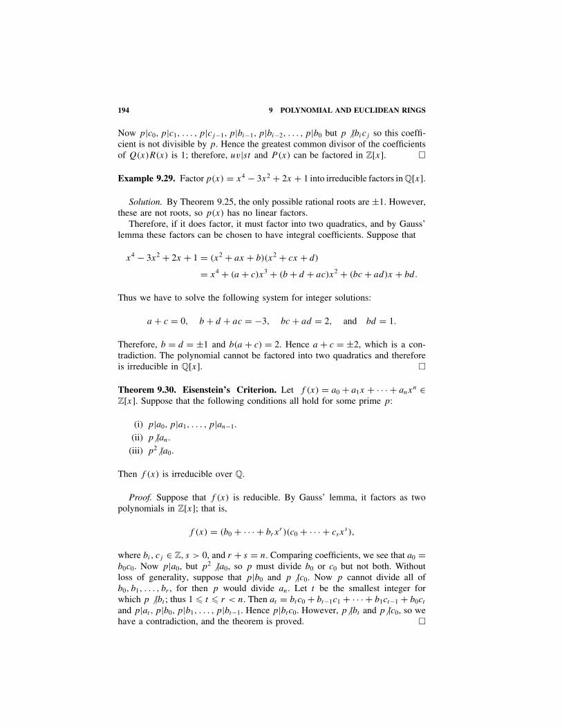
194 9 POLYNOMIAL AND EUCLIDEAN RINGS
Now p|c0, p|c1, . . . , p|cj−1, p|bi−1, p|bi−2, . . . , p|b0 but p � |bicj so this coeffi-cient is not divisible by p. Hence the greatest common divisor of the coefficientsof Q(x)R(x) is 1; therefore, uv|st and P(x) can be factored in Z[x]. �
Example 9.29. Factor p(x) = x4 − 3x2 + 2x + 1 into irreducible factors in Q[x].
Solution. By Theorem 9.25, the only possible rational roots are ±1. However,these are not roots, so p(x) has no linear factors.
Therefore, if it does factor, it must factor into two quadratics, and by Gauss’lemma these factors can be chosen to have integral coefficients. Suppose that
x4 − 3x2 + 2x + 1 = (x2 + ax + b)(x2 + cx + d)
= x4 + (a + c)x3 + (b + d + ac)x2 + (bc + ad)x + bd.
Thus we have to solve the following system for integer solutions:
a + c = 0, b + d + ac = −3, bc + ad = 2, and bd = 1.
Therefore, b = d = ±1 and b(a + c) = 2. Hence a + c = ±2, which is a con-tradiction. The polynomial cannot be factored into two quadratics and thereforeis irreducible in Q[x]. �
Theorem 9.30. Eisenstein’s Criterion. Let f (x) = a0 + a1x + · · · + anxn ∈
Z[x]. Suppose that the following conditions all hold for some prime p:
(i) p|a0, p|a1, . . . , p|an−1.
(ii) p � |an.
(iii) p2 � |a0.
Then f (x) is irreducible over Q.
Proof. Suppose that f (x) is reducible. By Gauss’ lemma, it factors as twopolynomials in Z[x]; that is,
f (x) = (b0 + · · · + brxr )(c0 + · · · + csx
s),
where bi, cj ∈ Z, s > 0, and r + s = n. Comparing coefficients, we see that a0 =b0c0. Now p|a0, but p2 � |a0, so p must divide b0 or c0 but not both. Withoutloss of generality, suppose that p|b0 and p � |c0. Now p cannot divide all ofb0, b1, . . . , br , for then p would divide an. Let t be the smallest integer forwhich p � |bt ; thus 1 � t � r < n. Then at = btc0 + bt−1c1 + · · · + b1ct−1 + b0ct
and p|at , p|b0, p|b1, . . . , p|bt−1. Hence p|btc0. However, p � |bt and p � |c0, so wehave a contradiction, and the theorem is proved. �

FACTORING POLYNOMIALS OVER FINITE FIELDS 195
For example, Eisenstein’s criterion can be used to show that x5 − 2,x7 + 2x3 + 12x2 − 2 and 2x3 + 9x − 3 are all irreducible over Q.
Example 9.31. Show that φ(x) = xp−1 + xp−2 + · · · + x + 1 is irreducible overQ for any prime p. This is called a cyclotomic polynomial and can be writtenφ(x) = (xp − 1)/(x − 1).
Solution. We cannot apply Eisenstein’s criterion to φ(x) as it stands. However,if we put x = y + 1, we obtain
φ(y + 1) = 1
y[(y + 1)p − 1]
= yp−1 +(
p
p − 1
)yp−2 +
(p
p − 2
)yp−3 + · · · +
(p
2
)y + p
where
(p
k
)= p!
k!(p − k)!is the binomial coefficient. Hence p divides
k!(p − k)!
(p
k
). If 1 � k � p − 1, the prime p does not divide k!(p − k)!, so
it must divide
(p
k
). Hence φ(y + 1) is irreducible by Eisenstein’s criterion, so
φ(x) is irreducible. �
FACTORING POLYNOMIALS OVER FINITE FIELDS
The roots of a polynomial in Zp[x] can be found by trying all the p possi-ble values.
Example 9.32. Does x4 + 4 ∈ Z7[x] have any roots in Z7?
Solution. We see from Table 9.3 that x4 + 4 is never zero and therefore hasno roots in Z7. �
Proposition 9.33. A polynomial in Z2[x] has a factor x + 1 if and only if it hasan even number of nonzero coefficients.
Proof. Let p(x) = a0 + a1x + · · · + anxn ∈ Z2[x]. By the factor theorem,
(x + 1) is a factor of p(x) if and only if p(1) = 0. (Remember that x − 1 = x + 1
TABLE 9.3. Values Modulo 7
x 0 1 2 3 4 5 6
x4 0 1 2 4 4 2 1
x4 + 4 4 5 6 1 1 6 5
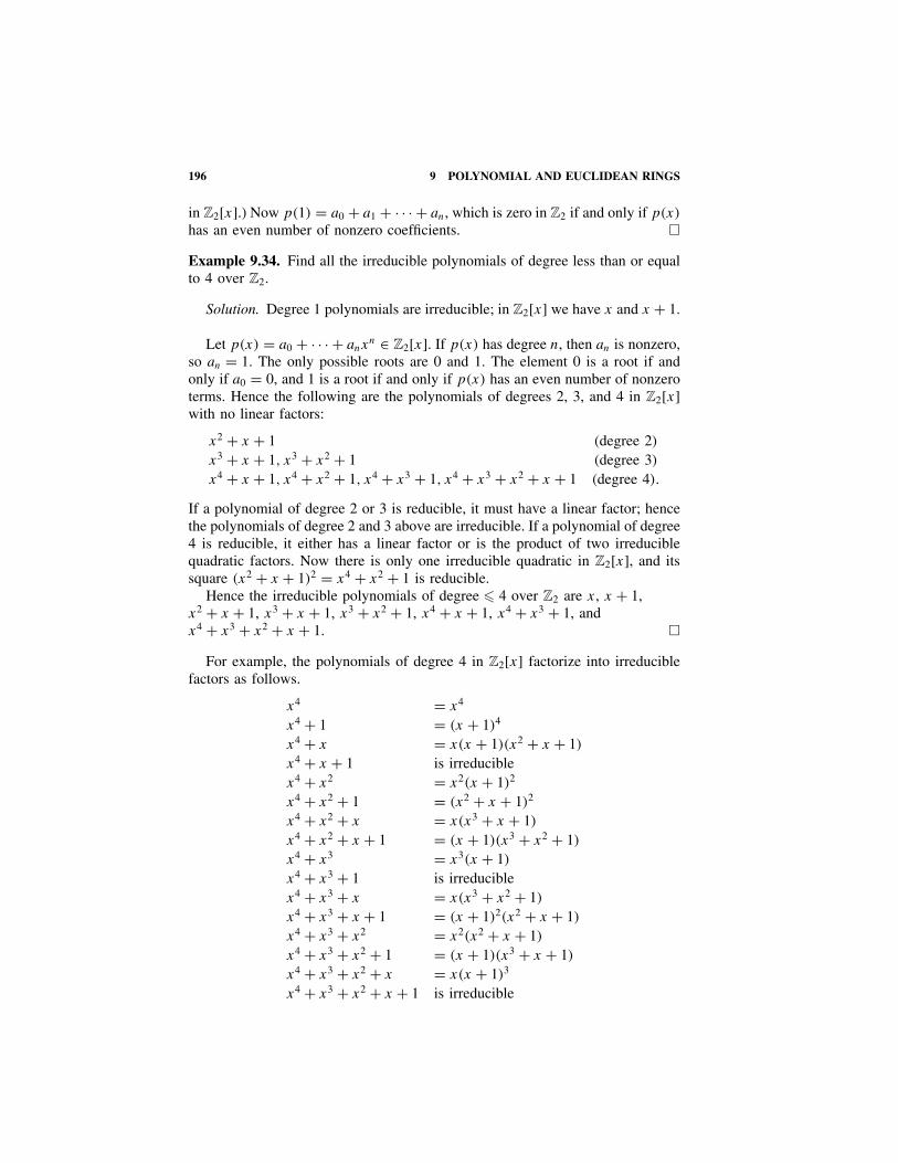
196 9 POLYNOMIAL AND EUCLIDEAN RINGS
in Z2[x].) Now p(1) = a0 + a1 + · · · + an, which is zero in Z2 if and only if p(x)
has an even number of nonzero coefficients. �
Example 9.34. Find all the irreducible polynomials of degree less than or equalto 4 over Z2.
Solution. Degree 1 polynomials are irreducible; in Z2[x] we have x and x + 1.
Let p(x) = a0 + · · · + anxn ∈ Z2[x]. If p(x) has degree n, then an is nonzero,
so an = 1. The only possible roots are 0 and 1. The element 0 is a root if andonly if a0 = 0, and 1 is a root if and only if p(x) has an even number of nonzeroterms. Hence the following are the polynomials of degrees 2, 3, and 4 in Z2[x]with no linear factors:
x2 + x + 1 (degree 2)
x3 + x + 1, x3 + x2 + 1 (degree 3)
x4 + x + 1, x4 + x2 + 1, x4 + x3 + 1, x4 + x3 + x2 + x + 1 (degree 4).
If a polynomial of degree 2 or 3 is reducible, it must have a linear factor; hencethe polynomials of degree 2 and 3 above are irreducible. If a polynomial of degree4 is reducible, it either has a linear factor or is the product of two irreduciblequadratic factors. Now there is only one irreducible quadratic in Z2[x], and itssquare (x2 + x + 1)2 = x4 + x2 + 1 is reducible.
Hence the irreducible polynomials of degree � 4 over Z2 are x, x + 1,x2 + x + 1, x3 + x + 1, x3 + x2 + 1, x4 + x + 1, x4 + x3 + 1, andx4 + x3 + x2 + x + 1. �
For example, the polynomials of degree 4 in Z2[x] factorize into irreduciblefactors as follows.
x4 = x4
x4 + 1 = (x + 1)4
x4 + x = x(x + 1)(x2 + x + 1)
x4 + x + 1 is irreduciblex4 + x2 = x2(x + 1)2
x4 + x2 + 1 = (x2 + x + 1)2
x4 + x2 + x = x(x3 + x + 1)
x4 + x2 + x + 1 = (x + 1)(x3 + x2 + 1)
x4 + x3 = x3(x + 1)
x4 + x3 + 1 is irreduciblex4 + x3 + x = x(x3 + x2 + 1)
x4 + x3 + x + 1 = (x + 1)2(x2 + x + 1)
x4 + x3 + x2 = x2(x2 + x + 1)
x4 + x3 + x2 + 1 = (x + 1)(x3 + x + 1)
x4 + x3 + x2 + x = x(x + 1)3
x4 + x3 + x2 + x + 1 is irreducible
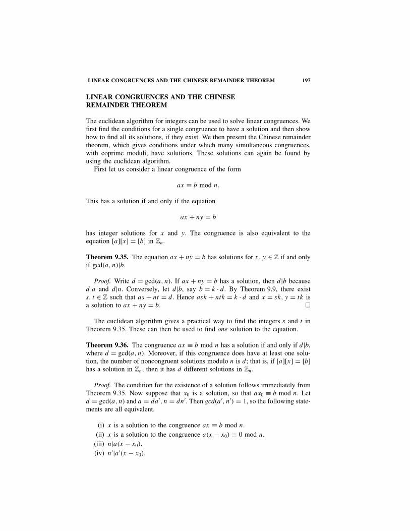
LINEAR CONGRUENCES AND THE CHINESE REMAINDER THEOREM 197
LINEAR CONGRUENCES AND THE CHINESEREMAINDER THEOREM
The euclidean algorithm for integers can be used to solve linear congruences. Wefirst find the conditions for a single congruence to have a solution and then showhow to find all its solutions, if they exist. We then present the Chinese remaindertheorem, which gives conditions under which many simultaneous congruences,with coprime moduli, have solutions. These solutions can again be found byusing the euclidean algorithm.
First let us consider a linear congruence of the form
ax ≡ b mod n.
This has a solution if and only if the equation
ax + ny = b
has integer solutions for x and y. The congruence is also equivalent to theequation [a][x] = [b] in Zn.
Theorem 9.35. The equation ax + ny = b has solutions for x, y ∈ Z if and onlyif gcd(a, n)|b.
Proof. Write d = gcd(a, n). If ax + ny = b has a solution, then d|b becaused|a and d|n. Conversely, let d|b, say b = k · d . By Theorem 9.9, there exists, t ∈ Z such that as + nt = d . Hence ask + ntk = k · d and x = sk, y = tk isa solution to ax + ny = b. �
The euclidean algorithm gives a practical way to find the integers s and t inTheorem 9.35. These can then be used to find one solution to the equation.
Theorem 9.36. The congruence ax ≡ b mod n has a solution if and only if d|b,where d = gcd(a, n). Moreover, if this congruence does have at least one solu-tion, the number of noncongruent solutions modulo n is d; that is, if [a][x] = [b]has a solution in Zn, then it has d different solutions in Zn.
Proof. The condition for the existence of a solution follows immediately fromTheorem 9.35. Now suppose that x0 is a solution, so that ax0 ≡ b mod n. Letd = gcd(a, n) and a = da′, n = dn′. Then gcd(a′, n′) = 1, so the following state-ments are all equivalent.
(i) x is a solution to the congruence ax ≡ b mod n.(ii) x is a solution to the congruence a(x − x0) ≡ 0 mod n.
(iii) n|a(x − x0).(iv) n′|a′(x − x0).
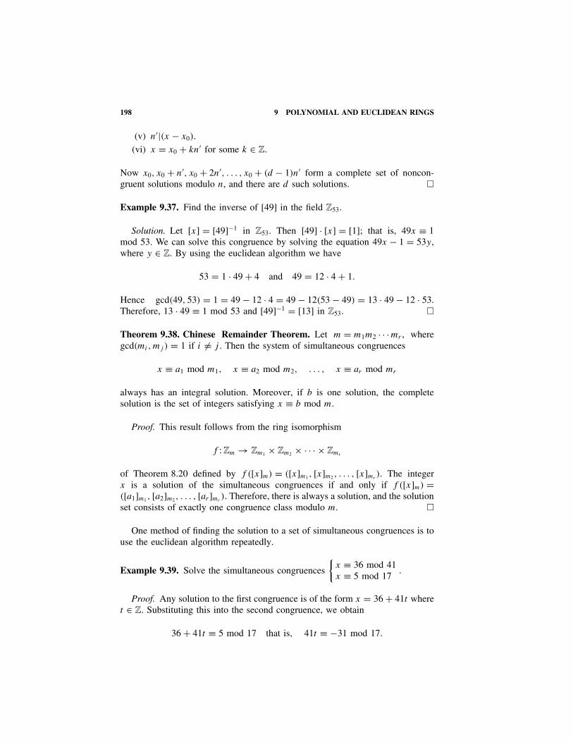
198 9 POLYNOMIAL AND EUCLIDEAN RINGS
(v) n′|(x − x0).(vi) x = x0 + kn′ for some k ∈ Z.
Now x0, x0 + n′, x0 + 2n′, . . . , x0 + (d − 1)n′ form a complete set of noncon-gruent solutions modulo n, and there are d such solutions. �
Example 9.37. Find the inverse of [49] in the field Z53.
Solution. Let [x] = [49]−1 in Z53. Then [49] · [x] = [1]; that is, 49x ≡ 1mod 53. We can solve this congruence by solving the equation 49x − 1 = 53y,where y ∈ Z. By using the euclidean algorithm we have
53 = 1 · 49 + 4 and 49 = 12 · 4 + 1.
Hence gcd(49, 53) = 1 = 49 − 12 · 4 = 49 − 12(53 − 49) = 13 · 49 − 12 · 53.Therefore, 13 · 49 ≡ 1 mod 53 and [49]−1 = [13] in Z53. �
Theorem 9.38. Chinese Remainder Theorem. Let m = m1m2 · · ·mr , wheregcd(mi,mj ) = 1 if i �= j . Then the system of simultaneous congruences
x ≡ a1 mod m1, x ≡ a2 mod m2, . . . , x ≡ ar mod mr
always has an integral solution. Moreover, if b is one solution, the completesolution is the set of integers satisfying x ≡ b mod m.
Proof. This result follows from the ring isomorphism
f : Zm → Zm1 × Zm2 × · · · × Zmr
of Theorem 8.20 defined by f ([x]m) = ([x]m1, [x]m2, . . . , [x]mr). The integer
x is a solution of the simultaneous congruences if and only if f ([x]m) =([a1]m1, [a2]m2, . . . , [ar ]mr
). Therefore, there is always a solution, and the solutionset consists of exactly one congruence class modulo m. �
One method of finding the solution to a set of simultaneous congruences is touse the euclidean algorithm repeatedly.
Example 9.39. Solve the simultaneous congruences
{x ≡ 36 mod 41x ≡ 5 mod 17
.
Proof. Any solution to the first congruence is of the form x = 36 + 41t wheret ∈ Z. Substituting this into the second congruence, we obtain
36 + 41t ≡ 5 mod 17 that is, 41t ≡ −31 mod 17.
LINEAR CONGRUENCES AND THE CHINESE REMAINDER THEOREM 199
Reducing modulo 17, we have 7t ≡ 3 mod 17. Solving this by the euclideanalgorithm, we have
17 = 2 · 7 + 3 and 7 = 2 · 3 + 1.
Therefore, 1 = 7 − 2(17 − 2 · 7) = 7 · 5 − 17 · 2 and 7 · 5 ≡ 1 mod 17. Hence7 · 15 ≡ 3 mod 17, so t ≡ 15 mod 17 is the solution to 7t ≡ 3 mod 17.
We have shown that if x = 36 + 41t is a solution to both congruences, thent = 15 + 17u, where u ∈ Z. That is,
x = 36 + 41t = 36 + 41(15 + 17u) = 651 + 697u
or x ≡ 651 mod 697 is the complete solution. �
Example 9.40. Find the smallest positive integer that has remainders 4, 3, and1 when divided by 5, 7, and 9, respectively.
Solution. We have to solve the three simultaneous congruences
x ≡ 4 mod 5, x ≡ 3 mod 7, and x ≡ 1 mod 9.
The first congruence implies that x = 4 + 5t , where t ∈ Z. Substituting into thesecond congruence, we have
4 + 5t ≡ 3 mod 7.
Hence 5t ≡ −1 mod 7. Now 5−1 = 3 in Z7, so t ≡ 3 · (−1) ≡ 4 mod 7. There-fore, t = 4 + 7u, where u ∈ Z, and any integer satisfying the first two congru-ences is of the form
x = 4 + 5t = 4 + 5(4 + 7u) = 24 + 35u.
Substituting this into the third congruence, we have 24 + 35u ≡ 1 mod 9 and−u ≡ −23 mod 9. Thus u ≡ 5 mod 9 and u = 5 + 9v for some v ∈ Z.
Hence any solution of the three congruences is of the form
x = 24 + 35u = 24 + 35(5 + 9v) = 199 + 315v.
The smallest positive solution is x = 199. �
The Chinese remainder theorem was known to ancient Chinese astronomers,who used it to date events from observations of various periodic astronomicalphenomena. It is used in this computer age as a tool for finding integer solutionsto integer equations and for speeding up arithmetic operations in a computer.
Addition of two numbers in conventional representation has to be carried outsequentially on the digits in each position; the digits in the ith position have to

200 9 POLYNOMIAL AND EUCLIDEAN RINGS
be added before the digit to be carried over to the (i + 1)st position is known.One method of speeding up addition on a computer is to perform addition usingresidue representation, since this avoids delays due to carry digits.
Let m = m1m2 · · · mr , where the integers mi are coprime in pairs. The residuerepresentation or modular representation of any number x in Zm is the r-tuple(a1, a2, . . . , ar), where x ≡ ai mod mi .
For example, every integer from 0 to 29 can be uniquely represented by itsresidues modulo 2, 3, and 5 in Table 9.4.
This residue representation corresponds exactly to the isomorphism
Z30 → Z2 × Z3 × Z5.
Since this is a ring isomorphism, addition and multiplication are performed simplyby adding and multiplying each residue separately.
For example, to add 4 and 7 using residue representation, we have
(0, 1, 4) + (1, 1, 2) = (0 + 1, 1 + 1, 4 + 2) = (1, 2, 1).
Similarly, multiplying 4 and 7, we have
(0, 1, 4) · (1, 1, 2) = (0 · 1, 1 · 1, 4 · 2) = (0, 1, 3).
Fast adders can be designed using residue representation, because all theresidues can be added simultaneously. Numbers can be converted easily intoresidue form; however, the reverse procedure of finding a number with a givenresidue representation requires the Chinese remainder theorem. See Knuth [19,Sec. 4.3.2] for further discussion of the use of residue representations in com-puters.
TABLE 9.4. Residue Representation of the Integersfrom 0 to 29
Residues Residues ResiduesModulo: Modulo: Modulo:
x 2 3 5 x 2 3 5 x 2 3 5
0 0 0 0 10 0 1 0 20 0 2 01 1 1 1 11 1 2 1 21 1 0 12 0 2 2 12 0 0 2 22 0 1 23 1 0 3 13 1 1 3 23 1 2 34 0 1 4 14 0 2 4 24 0 0 45 1 2 0 15 1 0 0 25 1 1 06 0 0 1 16 0 1 1 26 0 2 17 1 1 2 17 1 2 2 27 1 0 28 0 2 3 18 0 0 3 28 0 1 39 1 0 4 19 1 1 4 29 1 2 4
EXERCISES 201
EXERCISES
For Exercises 9.1 to 9.6 calculate the quotients and remainders.
9.1. Divide 3x4 + 4x3 − x2 + 5x − 1 by 2x2 + x + 1 in Q[x].9.2. Divide x6 + x4 − 4x3 + 5x by x3 + 2x2 + 1 in R[x].9.3. Divide x7 + x6 + x4 + x + 1 by x3 + x + 1 in Z2[x].9.4. Divide 2x5 + x4 + 2x3 + x2 + 2 by x3 + 2x + 2 in Z3[x].9.5. Divide 17 + 11i by 3 + 4i in Z[i].9.6. Divide 20 + 8i by 7 − 2i in Z[i].
For Exercises 9.7 to 9.13, find the greatest common divisors of the elements a, bin the given euclidean ring, and find elements s, t in the ring so that as + bt =gcd(a, b).
9.7. a = 33, b = 42 in Z.9.8. a = 2891, b = 1589 in Z.9.9. a = 2x3 − 4x2 − 8x + 1, b = 2x3 − 5x2 − 5x + 2 ∈ Q[x].
9.10. a = x6 − x3 − 16x2 + 12x − 2, b = x5 − 2x2 − 16x + 8 ∈ Q[x].9.11. a = x4 + x + 1, b = x3 + x2 + x ∈ Z3[x].9.12. a = x4 + 2, b = x3 + 3 ∈ Z5[x].9.13. a = 4 − i, b = 1 + i ∈ Z[i].
For Exercises 9.14 to 9.17, find one solution to each equation with x, y ∈ Z.
9.14. 15x + 36y = 3. 9.15. 24x + 29y = 1.9.16. 24x + 29y = 6. 9.17. 11x + 31y = 1.
For Exercises 9.18 to 9.21, find the inverse to the element in the given field.
9.18. [4] in Z7. 9.19. [24] in Z29.9.20. [35] in Z101. 9.21. [11] in Z31.
Find all integral solutions to the equations in Exercises 9.22 to 9.24.
9.22. 27x + 15y = 13. 9.23. 12x + 20y = 14.9.24. 28x + 20y = 16.
Factor the polynomials in Exercises 9.25 to 9.36 into irreducible factors in thegiven ring.
9.25. x5 − 1 in Q[x]. 9.26. x5 + 1 in Z2[x].9.27. x4 + 1 in Z5[x]. 9.28. 2x3 + x2 + 4x + 2 in Q[x].9.29. x4 − 9x + 3 in Q[x]. 9.30. 2x3 + x2 + 4x + 2 in C[x].9.31. x3 − 4x + 1 in Q[x]. 9.32. x4 + 3x3 + 9x − 9 in Q[x].9.33. x8 − 16 in C[x]. 9.34. x8 − 16 ∈ R[x].9.35. x8 − 16 in Q[x]. 9.36. x8 − 16 ∈ Z17[x].9.37. Find all irreducible polynomials of degree 5 over Z2.

202 9 POLYNOMIAL AND EUCLIDEAN RINGS
9.38. Find an irreducible polynomial of degree 2 over Z5.9.39. Find an irreducible polynomial of degree 3 over Z7.9.40. Find the kernel and image of the ring morphism ψ : R[x] → C defined by
ψ(p(x)) = p(i), where i = √−1.9.41. Find the kernel and image of the ring morphism ψ : R[x] → C defined by
ψ(p(x)) = p(1 + √3i).
In Exercises 9.42 to 9.47, are the polynomials irreducible in the given ring?Give reasons.
9.42. x3 + x2 + x + 1 in Q[x].9.43. 3x8 − 4x6 + 8x5 − 10x + 6 in Q[x].9.44. x4 + x2 − 6 in Q[x]. 9.45. 4x3 + 3x2 + x + 1 in Z5[x].9.46. x5 + 15 in Q[x]. 9.47. x4 − 2x3 + x2 + 1 in R[x].9.48. Is Z[x] a euclidean ring when δ(f (x)) = degf (x) for any nonzero poly-
nomial? Is Z[x] a euclidean ring with any other definition of δ(f (x))?9.49. Can you define a division algorithm in R[x, y]? How would you divide
x3 + 3xy + y + 4 by xy + y3 + 2?9.50. Let Lp be the set of all linear functions f : Zp → Zp of the form f (x) =
ax + b, where a �= 0 in Zp. Show that (Lp, Ž ) is a group of order p(p − 1)
under composition.9.51. If p is a prime, prove that (x − a)|(xp−1 − 1) in Zp[x] for all nonzero a
in Zp. Hence prove that
xp−1 − 1 = (x − 1)(x − 2) · · · (x − p + 1) in Zp[x].
9.52. (Wilson’s theorem) Prove that (n − 1)! ≡ −1 mod n if and only if n
is prime.
9.53. Prove that√
2/3√
5 is irrational.
9.54. Find a polynomial in Q[x] with√
2 + √3 as a root. Then prove that√
2 + √3 is irrational.
9.55. Is 5 irreducible in Z[i]?9.56. Show that Z[
√−5] = {a + b√−5|a, b ∈ Z} does not have the unique fac-
torization property.9.57. Prove that a gaussian integer is irreducible if and only if it is an invertible
element times one of the following gaussian integers:(1) any prime p in Z with p ≡ 3 mod 4.(2) 1 + i.(3) a + bi, where a is positive and even, and a2 + b2 = p, for some prime
p in Z such that p ≡ 1 mod 4.9.58. If r/s is a rational root, in its lowest terms, of a polynomial p(x) with
integral coefficients, show that p(x) = (sx − r)g(x) for some polynomialg(x) with integral coefficients.

EXERCISES 203
9.59. Prove that r/s, in its lowest terms, cannot be a root of the integral poly-nomial p(x) unless (s − r)|p(1). This can be used to shorten the list ofpossible rational roots of an integral polynomial.
9.60. Let m = m1m2 · · · mr and Mi = m/mi . If gcd(mi,mj ) = 1 for i �= j , eachof the congruences Miy ≡ 1 mod mi has a solution y ≡ bi mod mi . Provethat the solution to the simultaneous congruences
x ≡ a1 mod m1, x ≡ a2 mod m2, . . . , x ≡ ar mod mr
is x ≡ ∑ri=1 Mibiai mod m.
For Exercises 9.61 to 9.64, solve the simultaneous congruences.
9.61. x ≡ 5 mod 7 9.62. x ≡ 41 mod 65x ≡ 4 mod 6. x ≡ 35 mod 72.
9.63. x ≡ 0 mod 2 9.64. x ≡ 9 mod 12x ≡ 1 mod 3 x ≡ 3 mod 13x ≡ 2 mod 5. x ≡ 6 mod 25.
9.65. Prove that det
320 461 5264 72702 1008 −967 −44−91 2333 46 127164 −216 1862 469
is nonzero.
9.66. Solve the following simultaneous equations:
26x − 141y = −697
55x − 112y = 202
(a) in Z2, (b) in Z3, and (c) in Z5. Then use the Chinese remainder theoremto solve them in Z assuming they have a pair of integral solutions between0 and 29.
9.67. The value of det
676 117 522
375 65 290825 143 639
is positive and less than 100.
Find its value without using a calculator. (If you get tired of doing arith-metic, calculate its value mod 10 and mod 11 and then use the Chineseremainder theorem.)
9.68. The polynomial x3 + 5x ∈ Z6[x] has six roots. Does this contradict Theo-rem 9.6?
9.69. If R is an integral domain and R[x] is euclidean, show that R must bea field.
9.70. Assume that R is a euclidean domain in which δ(a + b) � max{δ(a), δ(b)}whenever a, b, and a + b are all nonzero. Show that the quotient andremainder in the division algorithm are uniquely determined.

10QUOTIENT RINGS
In this chapter we define a quotient ring in a way similar to our definition ofa quotient group. The analogue of a normal subgroup is called an ideal, anda quotient ring consists of the set of cosets of the ring by one of its ideals.As in groups, we have a morphism theorem connecting morphisms, ideals, andquotient rings. We discover under what conditions quotient rings are fields. Thiswill enable us to fulfill our long-range goal of extending the number systems bydefining new fields using quotient rings of some familiar rings.
IDEALS AND QUOTIENT RINGS
If (R, +, ·) is any ring and (S, +) is any subgroup of the abelian group (R, +),then the quotient group (R/S, +) has already been defined. However, R/S doesnot have a ring structure induced on it by R unless S is a special kind of subgroupcalled an ideal.
A nonempty subset I of a ring R is called an ideal of R if the followingconditions are satisfied for all x, y ∈ I and r ∈ R:
(i) x − y ∈ I .(ii) x · r and r · x ∈ I .
Condition (i) implies that (I, +) is a subgroup of (R, +). In any ring R, R itselfis an ideal, and {0} is an ideal.
Proposition 10.1. Let a be an element of a commutative ring R. The set{ar|r ∈ R} of all multiples of a is an ideal of R called the principal idealgenerated by a. This ideal is denoted by (a).
Proof. Let ar, as ∈ (a) and t ∈ R. Then ar − as = a(r − s) ∈ (a) and (ar)t =a(rt) ∈ (a). Hence (a) is an ideal of R. �
Modern Algebra with Applications, Second Edition, by William J. Gilbert and W. Keith NicholsonISBN 0-471-41451-4 Copyright 2004 John Wiley & Sons, Inc.
204
IDEALS AND QUOTIENT RINGS 205
For example, (n) = nZ, consisting of all integer multiples of n, is the principalideal generated by n in Z.
The set of all polynomials in Q[x] that contain x2 − 2 as a factor is theprincipal ideal (x2 − 2) = {(x2 − 2) · p(x)|p(x) ∈ Q[x]} generated by x2 − 2 inQ[x]. The set of all real polynomials that have zero constant term is the principalideal (x) = {x · p(x)|p(x) ∈ R[x]} generated by x in R[x]. It is also the set ofreal polynomials with 0 as a root.
The set of all real polynomials, in two variables x and y, that have a zeroconstant term is an ideal of R[x, y]. However, this ideal is not principal (seeExercise 10.30).
However, every ideal is principal in many commutative rings; these are calledprincipal ideal rings.
Theorem 10.2. A euclidean ring is a principal ideal ring.
Proof. Let I be any ideal of the euclidean ring R. If I = {0}, then I = (0),the principal ideal generated by 0. Otherwise, I contains nonzero elements. Letb be a nonzero element of I for which δ(b) is minimal. If a is any other elementin I , then, by the division algorithm, there exist q, r ∈ R such that
a = q · b + r where r = 0 or δ(r) < δ(b).
Now r = a − q · b ∈ I . Since b is a nonzero element of I for which δ(b) isminimal, it follows that r must be zero and a = q · b. Therefore, a ∈ (b) andI ⊆ (b).
Conversely, any element of (b) is of the form q · b for some q ∈ R, so q · b ∈I . Therefore, I ⊇ (b), which proves that I = (b). Hence R is a principal idealring. �
Corollary 10.3. Z is a principal ideal ring, so is F [x], if F is a field.
Proof. This follows because Z and F [x] are euclidean rings. �
Proposition 10.4. Let I be ideal of the ring R. If I contains the identity 1, thenI is the entire ring R.
Proof. Let 1 ∈ I and r ∈ R. Then r = r · 1 ∈ I , so I = R. �
Let I be any ideal in a ring R. Then (I, +) is a normal subgroup of (R, +),and we denote the coset of I in R that contains r by I + r . Hence
I + r = {i + r ∈ R|i ∈ I }.The cosets of I in R are the equivalence classes under the congruence relationmodulo I . We have
r1 ≡ r2 modI if and only if r1 − r2 ∈ I.

206 10 QUOTIENT RINGS
By Theorem 4.18, the set of cosets R/I = {I + r|r ∈ R} is an abelian groupunder the operation defined by
(I + r1) + (I + r2) = I + (r1 + r2).
In fact, we get a ring structure in R/I .
Theorem 10.5. Let I be an ideal in the ring R. Then the set of cosets forms aring (R/I, +, ·) under the operations defined by
(I + r1) + (I + r2) = I + (r1 + r2)
and(I + r1)(I + r2) = I + (r1r2).
This ring (R/I, +, ·) is called the quotient ring (or factor ring) of R by I .
Proof. As mentioned above, (R/I, +) is an abelian group; thus we only haveto verify the axioms related to multiplication.
We first show that multiplication is well defined on cosets. Let I + r ′1 = I + r1
and I + r ′2 = I + r2, so that r ′
1 − r1 = i1 ∈ I and r ′2 − r2 = i2 ∈ I . Then
r ′1r
′2 = (i1 + r1)(i2 + r2) = i1i2 + r1i2 + i1r2 + r1r2.
Now, since I is an ideal, i1i2, r1i2 and i1r2 ∈ I . Hence r ′1r
′2 − r1r2 ∈ I , so
I + r ′1r
′2 = I + r1r2, which shows that multiplication is well defined on R/I .
Multiplication is associative and distributive over addition. If r1, r2, r3 ∈R, then
(I + r1){(I + r2)(I + r3)} = (I + r1)(I + r2r3) = I + r1(r2r3) = I + (r1r2)r3
= (I + r1r2)(I + r3) = {(I + r1)(I + r2)}(I + r3).
Also,
(I + r1){(I + r2) + (I + r3)} = (I + r1){I + (r2 + r3)} = I + r1(r2 + r3)
= I + (r1r2 + r1r3) = (I + r1r2) + (I + r1r3)
= {(I + r1)(I + r2)} + {(I + r1)(I + r3)}.
The other distributive law can be proved similarly. The multiplicative identity isI + 1. Hence (R/I, +, ·) is a ring. �

COMPUTATIONS IN QUOTIENT RINGS 207
TABLE 10.1. Quotient Ring Z6/{0, 2, 4}+ I I + 1 · I I + 1
I I I + 1 I I I
I + 1 I + 1 I I + 1 I I + 1
For example, the quotient ring of Z by (n) is Z/(n) = Zn, the ring of integersmodulo n. A coset (n) + r = {nz + r|z ∈ Z} is the equivalent class modulo n
containing r .If R is commutative, so is the quotient ring R/I , because
(I + r1)(I + r2) = I + r1r2 = I + r2r1 = (I + r2)(I + r1).
Example 10.6. If I = {0, 2, 4} is the ideal generated by 2 in Z6, find the tablesfor the quotient ring Z6/I .
Solution. There are two cosets of Z6 by I : namely, I = {0, 2, 4} and I + 1 ={1, 3, 5}. Hence
Z6/I = {I, I + 1}.
The addition and multiplication tables given in Table 10.1 show that the quotientring Z6/I is isomorphic to Z2. �
COMPUTATIONS IN QUOTIENT RINGS
If F is a field, the quotient rings of the polynomial ring F [x] form an importantclass of rings that will be used to construct new fields. Recall that F [x] is aprincipal ideal ring, so that any quotient ring is of the form F [x]/(p(x)), for somepolynomial p(x) ∈ F [x]. We now look at the structure of such a quotient ring.
The elements of the ring F [x]/(p(x)) are equivalence classes under the rela-tion on F [x] defined by
f (x) ≡ g(x) mod(p(x)) if and only if f (x) − g(x) ∈ (p(x)).
Lemma 10.7. f (x) ≡ g(x) mod(p(x)) if and only if f (x) and g(x) have thesame remainder when divided by p(x).
Proof. Let f (x) = q(x) · p(x) + r(x) and g(x) = s(x) · p(x) + t (x), wherer(x) and t(x) are zero or have degrees less than that of p(x). Now the lemmafollows because the following statements are equivalent:
(i) f (x) ≡ g(x) mod(p(x)).(ii) f (x) − g(x) ∈ (p(x)).
(iii) p(x)|f (x) − g(x).
208 10 QUOTIENT RINGS
(iv) p(x)|[{q(x) − s(x)} · p(x) + (r(x) − t (x))].(v) p(x)|[r(x) − t (x)].
(vi) r(x) = t (x). �
Hence every coset of F [x] by (p(x)) contains the zero polynomial or a poly-nomial of degree less than that of p(x).
Theorem 10.8. If F is a field, let P be the ideal (p(x)) in F [x] generated bythe polynomial p(x) of degree n > 0. The different elements of F [x]/(p(x)) areprecisely those of the form
P + a0 + a1x + · · · + an−1xn−1 where a0, a1, . . . , an−1 ∈ F.
Proof. Let P + f (x) be any element of F [x]/(p(x)) and let r(x) be theremainder when f (x) is divided by p(x). Then, by Lemma 10.7, P + f (x) =P + r(x), which is of the required form.
Suppose that P + r(x) = P + t (x), where r(x) and t (x) are zero or havedegree less than n. Then
r(x) ≡ t (x) mod(p(x)),
and by Lemma 10.7, r(x) = t (x). �
Example 10.9. Write down the tables for Z2[x]/(x2 + x + 1).
Solution. Let P = (x2 + x + 1), so that
Z2[x]/(x2 + x + 1) = {P + a0 + a1x|a0, a1 ∈ Z2}= {P,P + 1, P + x, P + x + 1}.
The tables for the quotient ring are given in Table 10.2. The addition table isstraightforward to calculate. Multiplication is computed as follows:
(P + x)2 = P + x2 = P + (x2 + x + 1) + (x + 1) = P + x + 1
and
(P + x)(P + x + 1) = P + x2 + x = P + (x2 + x + 1) + 1 = P + 1. �
Example 10.10. Let P = x2 − 2 be the principal ideal of Q[x] generated byx2 − 2. Find the sum and product of P + 3x + 4 and P + 5x − 6 in the ringQ[x]/(x2 − 2) = {P + a0 + a1x|a0, a1 ∈ Q}.
Solution. (P + 3x + 4) + (P + 5x − 6) = P + (3x + 4) + (5x − 6) = P +8x − 2. (P + 3x + 4)(P + 5x − 6) = P + (3x + 4)(5x − 6) = P + 15x2 + 2x
− 24. By the division algorithm, 15x2 + 2x − 24 = 15(x2 − 2) + 2x + 6. Hence,by Lemma 10.7, P + 15x2 + 2x − 24 = P + 2x + 6. �
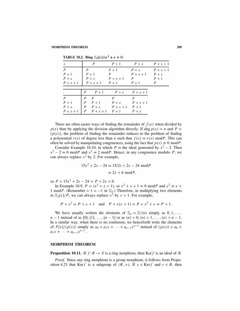
MORPHISM THEOREM 209
TABLE 10.2. Ring Z2[x ]/(x 2 + x + 1)
+ P P + 1 P + x P + x + 1
P P P + 1 P + x P + x + 1P + 1 P + 1 P P + x + 1 P + x
P + x P + x P + x + 1 P P + 1P + x + 1 P + x + 1 P + x P + 1 P
· P P + 1 P + x P + x + 1
P P P P P
P + 1 P P + 1 P + x P + x + 1P + x P P + x P + x + 1 P + 1P + x + 1 P P + x + 1 P + 1 P + x
There are often easier ways of finding the remainder of f (x) when divided byp(x) than by applying the division algorithm directly. If deg p(x) = n and P =(p(x)), the problem of finding the remainder reduces to the problem of findinga polynomial r(x) of degree less than n such that f (x) ≡ r(x) modP . This canoften be solved by manipulating congruences, using the fact that p(x) ≡ 0 modP .
Consider Example 10.10, in which P is the ideal generated by x2 − 2. Thenx2 − 2 ≡ 0 modP and x2 ≡ 2 modP . Hence, in any congruence modulo P , wecan always replace x2 by 2. For example,
15x2 + 2x − 24 ≡ 15(2) + 2x − 24 modP
≡ 2x + 6 modP,
so P + 15x2 + 2x − 24 = P + 2x + 6.In Example 10.9, P = (x2 + x + 1), so x2 + x + 1 ≡ 0 modP and x2 ≡ x +
1 modP . (Remember + 1 = −1 in Z2.) Therefore, in multiplying two elementsin Z2[x]/P , we can always replace x2 by x + 1. For example,
P + x2 = P + x + 1 and P + x(x + 1) = P + x2 + x = P + 1.
We have usually written the elements of Zn = Z/(n) simply as 0, 1, . . . ,
n − 1 instead of as [0], [1], . . . , [n − 1] or as (n) + 0, (n) + 1, . . . , (n) + n − 1.In a similar way, when there is no confusion, we henceforth write the elementsof F [x]/(p(x)) simply as a0 + a1x + · · · + an−1x
n−1 instead of (p(x)) + a0 +a1x + · · · + an−1x
n−1.
MORPHISM THEOREM
Proposition 10.11. If f : R → S is a ring morphism, then Kerf is an ideal of R.
Proof. Since any ring morphism is a group morphism, it follows from Propo-sition 4.23 that Kerf is a subgroup of (R, +). If x ∈ Kerf and r ∈ R, then
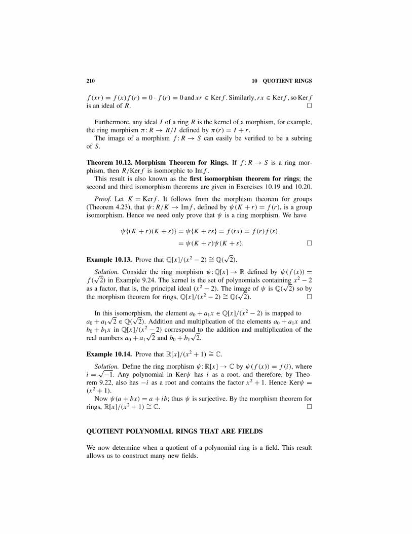
210 10 QUOTIENT RINGS
f (xr) = f (x)f (r) = 0 · f (r) = 0 and xr ∈ Kerf . Similarly, rx ∈ Kerf , so Kerfis an ideal of R. �
Furthermore, any ideal I of a ring R is the kernel of a morphism, for example,the ring morphism π : R → R/I defined by π(r) = I + r .
The image of a morphism f : R → S can easily be verified to be a subringof S.
Theorem 10.12. Morphism Theorem for Rings. If f : R → S is a ring mor-phism, then R/Kerf is isomorphic to Imf .
This result is also known as the first isomorphism theorem for rings; thesecond and third isomorphism theorems are given in Exercises 10.19 and 10.20.
Proof. Let K = Kerf . It follows from the morphism theorem for groups(Theorem 4.23), that ψ : R/K → Imf , defined by ψ(K + r) = f (r), is a groupisomorphism. Hence we need only prove that ψ is a ring morphism. We have
ψ{(K + r)(K + s)} = ψ{K + rs} = f (rs) = f (r)f (s)
= ψ(K + r)ψ(K + s). �
Example 10.13. Prove that Q[x]/(x2 − 2) ∼= Q(√
2).
Solution. Consider the ring morphism ψ : Q[x] → R defined by ψ(f (x)) =f (
√2) in Example 9.24. The kernel is the set of polynomials containing x2 − 2
as a factor, that is, the principal ideal (x2 − 2). The image of ψ is Q(√
2) so bythe morphism theorem for rings, Q[x]/(x2 − 2) ∼= Q(
√2). �
In this isomorphism, the element a0 + a1x ∈ Q[x]/(x2 − 2) is mapped toa0 + a1
√2 ∈ Q(
√2). Addition and multiplication of the elements a0 + a1x and
b0 + b1x in Q[x]/(x2 − 2) correspond to the addition and multiplication of thereal numbers a0 + a1
√2 and b0 + b1
√2.
Example 10.14. Prove that R[x]/(x2 + 1) ∼= C.
Solution. Define the ring morphism ψ : R[x] → C by ψ(f (x)) = f (i), wherei = √−1. Any polynomial in Kerψ has i as a root, and therefore, by Theo-rem 9.22, also has −i as a root and contains the factor x2 + 1. Hence Kerψ =(x2 + 1).
Now ψ(a + bx) = a + ib; thus ψ is surjective. By the morphism theorem forrings, R[x]/(x2 + 1) ∼= C. �
QUOTIENT POLYNOMIAL RINGS THAT ARE FIELDS
We now determine when a quotient of a polynomial ring is a field. This resultallows us to construct many new fields.

QUOTIENT POLYNOMIAL RINGS THAT ARE FIELDS 211
Theorem 10.15. Let a be an element of the euclidean ring R. The quotient ringR/(a) is a field if and only if a is irreducible in R.
Proof. Suppose that a is an irreducible element of R and let (a) + b be anonzero element of R/(a). Then b is not a multiple of a, and since a is irreducible,gcd(a, b) = 1. By Theorem 9.9, there exist s, t ∈ R such that
sa + tb = 1.
Now sa ∈ (a), so [(a) + t] · [(a) + b] = (a) + 1, the identity of R/(a). Hence(a) + t is the inverse of (a) + b in R/(a) and R/(a) is a field.
Now suppose that a is not irreducible in R so that there exist elements s andt , which are not invertible, with st = a. By Lemma 9.17, δ(s) < δ(st) = δ(a)
and δ(t) < δ(st) = δ(a). Hence s is not divisible by a, and s /∈ (a). Similarly,t /∈ (a), and neither (a) + s nor (a) + t is the zero element of R/(a). However,
[(a) + s] · [(a) + t] = (a) + st = (a), the zero element of R/(a).
Therefore, the ring R/(a) has zero divisors and cannot possibly be a field. �
For example, in the quotient ring Q[x]/P , where P = (x2 − 1), the elementsP + x + 1 and P + x − 1 are zero divisors because
(P + x + 1) · (P + x − 1) = P + x2 − 1 = P, the zero element.
Corollary 10.16. Zp = Z/(p) is a field if and only if p is prime.
Proof. This result, which we proved in Theorem 8.11, follows fromTheorem 10.15 because the irreducible elements in Z are the primes (andtheir negatives). �
Another particular case of Theorem 10.15 is the following important theorem.
Theorem 10.17. The ring F [x]/(p(x)) is a field if and only if p(x) is irreducibleover the field F . Furthermore, the ring F [x]/(p(x)) always contains a subringisomorphic to the field F .
Proof. The first part of the theorem is just Theorem 10.15. Let F = {(p(x)) +r|r ∈ F }. This can be verified to be a subring of F [x]/(p(x)), which is isomor-phic to the field F by the isomorphism that takes r ∈ F to (p(x))+r ∈ F [x]/(p(x)). �
Example 10.18. Show that Z2[x]/(x2 + x + 1) is a field with four elements.
Solution. We showed in Example 9.34 that x2 + x + 1 is irreducible over Z2
and in Example 10.9 that the quotient ring has four elements. Hence the quotientring is a field containing four elements. Its tables are given in Table 10.2. �

212 10 QUOTIENT RINGS
Example 10.19. Write down the multiplication table for the field Z3[x]/(x2 + 1).
Solution. If x = 0, 1, or 2 in Z3, then x2 + 1 = 1, 2, or 2; thus, by the factortheorem, x2 + 1 has no linear factors. Hence x2 + 1 is irreducible over Z3 and,by Theorem 10.17, the quotient ring Z3[x]/(x2 + 1) is a field. By Theorem 10.8,the elements of this field can be written as
Z3[x]/(x2 + 1) = {a0 + a1x|a0, a1 ∈ Z3}.
Hence the field contains nine elements. Its multiplication table is given inTable 10.3. This can be calculated by multiplying the polynomials in Z3[x] andreplacing x2 by −1 or 2, since x2 ≡ −1 ≡ 2mod (x2 + 1). �
Example 10.20. Show that Q[x]/(x3 − 5) = {a0 + a1x + a2x2|ai ∈ Q} is a field
and find the inverse of the element x + 1.
Solution. By the rational roots theorem (Theorem 9.25), (x3 − 5) has no linearfactors and hence is irreducible over Q. Therefore, by Theorem 10.17,Q[x]/(x3 − 5) is a field.
If s(x) is the inverse of x + 1, then (x + 1)s(x) ≡ 1 mod(x3 − 5); that is,(x + 1)s(x) + (x3 − 5)t (x) = 1 for some t (x) ∈ Q[x].
We can find such polynomials s(x) and t (x) by the euclidean algorithm. Wehave (see below)
x3 − 5 = (x2 − x + 1)(x + 1) − 6,
so6 ≡ (x2 − x + 1)(x + 1) mod(x3 − 5)
and1 ≡ 1
6 (x2 − x + 1)(x + 1) mod(x3 − 5).
TABLE 10.3. Multiplication in Z3[x ]/(x 2 + 1)
· 0 1 2 x x + 1 x + 2 2x 2x + 1 2x + 2
0 0 0 0 0 0 0 0 0 01 0 1 2 x x + 1 x + 2 2x 2x + 1 2x + 22 0 2 1 2x 2x + 2 2x + 1 x x + 2 x + 1x 0 x 2x 2 x + 2 2x + 2 1 x + 1 2x + 1x + 1 0 x + 1 2x + 2 x + 2 2x 1 2x + 1 2 x
x + 2 0 x + 2 2x + 1 2x + 2 1 x x + 1 2x 22x 0 2x x 1 2x + 1 x + 1 2 2x + 2 x + 22x + 1 0 2x + 1 x + 2 x + 1 2 2x 2x + 2 x 12x + 2 0 2x + 2 x + 1 2x + 1 x 2 x + 2 1 2x
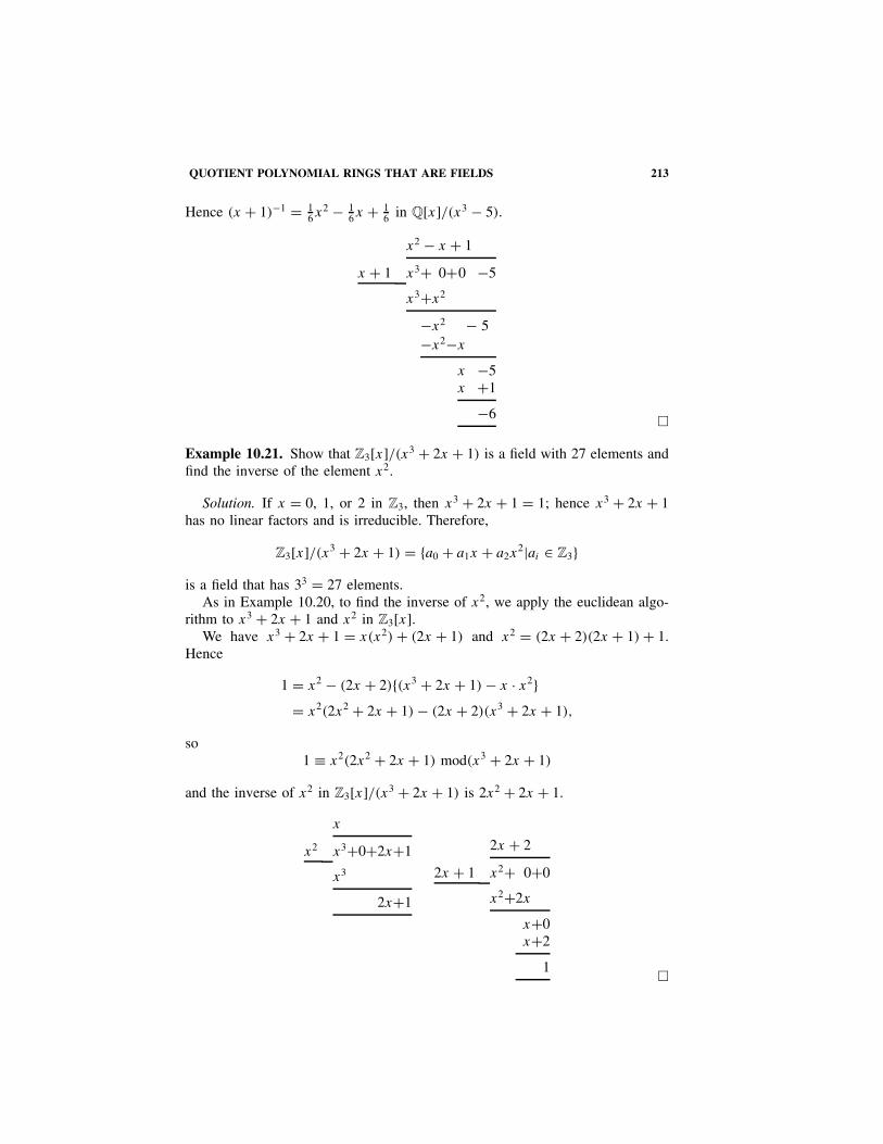
QUOTIENT POLYNOMIAL RINGS THAT ARE FIELDS 213
Hence (x + 1)−1 = 16x2 − 1
6x + 16 in Q[x]/(x3 − 5).
x2 − x + 1
x + 1 x3+ 0+0 −5
x3+x2
−x2 − 5−x2−x
x −5x +1
−6 �
Example 10.21. Show that Z3[x]/(x3 + 2x + 1) is a field with 27 elements andfind the inverse of the element x2.
Solution. If x = 0, 1, or 2 in Z3, then x3 + 2x + 1 = 1; hence x3 + 2x + 1has no linear factors and is irreducible. Therefore,
Z3[x]/(x3 + 2x + 1) = {a0 + a1x + a2x2|ai ∈ Z3}
is a field that has 33 = 27 elements.As in Example 10.20, to find the inverse of x2, we apply the euclidean algo-
rithm to x3 + 2x + 1 and x2 in Z3[x].We have x3 + 2x + 1 = x(x2) + (2x + 1) and x2 = (2x + 2)(2x + 1) + 1.
Hence
1 = x2 − (2x + 2){(x3 + 2x + 1) − x · x2}= x2(2x2 + 2x + 1) − (2x + 2)(x3 + 2x + 1),
so1 ≡ x2(2x2 + 2x + 1) mod(x3 + 2x + 1)
and the inverse of x2 in Z3[x]/(x3 + 2x + 1) is 2x2 + 2x + 1.
x
x2 x3+0+2x+1
x3
2x+1
2x + 2
2x + 1 x2+ 0+0
x2+2x
x+0x+2
1 �
214 10 QUOTIENT RINGS
We cannot use Theorem 10.15 directly on a field to obtain any new quotientfields, because the only ideals of a field are the zero ideal and the entire field. Infact, the following result shows that a field can be characterized by its ideals.
Theorem 10.22. The nontrivial commutative ring R is a field if and only if (0)and R are its only ideals.
Proof. Let I be an ideal in the field R. Suppose that I = (0), so that there isa nonzero element a ∈ I . Since a−1 ∈ R, a · a−1 = 1 ∈ I . Therefore, by Propo-sition 10.4, I = R. Hence R has only trivial ideals.
Conversely, suppose that (0) and R are the only ideals in the ring R. Leta be a nonzero element of R and consider (a) the principal ideal generatedby a. Since 1 · a ∈ (a), (a) = (0), and hence (a) = R. Hence 1 ∈ R = (a), sothere must exist some b ∈ R such that a · b = 1. Therefore, b = a−1 and R isa field. �
EXERCISES
For Exercises 10.1 to 10.6, find all the ideals in the rings.
10.1. Z2 × Z2. 10.2. Z18. 10.3. Q.10.4. Z7. 10.5. C[x]. 10.6. Z[i].
For Exercises 10.7 to 10.10, construct addition and multiplication tables for therings. Find all the zero divisors in each ring. Which of these rings are fields?
10.7. Z6/(3). 10.8. Z2[x]/(x3 + 1).10.9. Z3 × Z3/((1, 2)). 10.10. Z3[x]/(x2 + 2x + 2).
For Exercises 10.11 to 10.14, compute the sum and product of the elements in thegiven quotient rings.
10.11. 3x + 4 and 5x − 2 in Q[x]/(x2 − 7).10.12. x2 + 3x + 1 and −2x2 + 4 in Q[x]/(x3 + 2).10.13. x2 + 1 and x + 1 in Z2[x]/(x3 + x + 1).10.14. ax + b and cx + d in R[x]/(x2 + 1), where a, b, c, d ∈ R.10.15. If U and V are ideals in a ring R, prove that U ∩ V is also an ideal in
R.10.16. Show, by example, that if U and V are ideals in a ring R, then U ∪ V is
not necessarily an ideal in R. But prove that U + V = {u + v|u ∈ U, v ∈V } is always an ideal in R.
10.17. Find a generator of the following ideals in the given ring and prove ageneral result for the intersection of two ideals in a principal ideal ring.(a) (2) ∩ (3) in Z. (b) (12) ∩ (18) in Z.(c) (x2 − 1) ∩ (x + 1) in Q[x].

EXERCISES 215
10.18. Find a generator of the following ideals in the given ring and prove ageneral result for the sum of two ideals in a principal ideal ring.(a) (2) + (3) in Z. (b) (9) + (12) in Z.(c) (x2 + x + 1) + (x2 + 1) in Z2[x].
10.19. (Second isomorphism theorem for rings) If I and J are ideals of thering R, prove that
I/(I ∩ J ) ∼= (I + J )/J.
10.20. (Third isomorphism theorem for rings) Let I and J be two ideals ofthe ring R, with J ⊆ I . Prove that I/J is an ideal of R/J and that
(R/J )/(I/J ) ∼= R/I.
For Exercises 10.21 to 10.29, prove the isomorphisms.
10.21. R[x]/(x2 + 5) ∼= C.10.22. Z[x]/(x2 + 1) ∼= Z[i] = {a + ib|a, b ∈ Z}.10.23. Q[x]/(x2 − 7) ∼= Q(
√7) = {a + b
√7|a, b ∈ Q}.
10.24. Z[x]/(2x − 1) ∼= {a/b ∈ Q|a ∈ Z, b = 2r , r � 0}, a subring of Q.10.25. Z14/(7) ∼= Z7. 10.26. Z14/(2) ∼= Z2.10.27. R[x, y]/(x + y) ∼= R[y]. 10.28. (R × S)/((1, 0)) ∼= S.10.29. P (X)/P (X − Y ) ∼= P (Y ), where Y is a subset of X and the operations
in these boolean rings are symmetric difference and intersection.10.30. Let I be the set of all polynomials with no constant term in R[x, y]. Find
a ring morphism from R[x, y] to R whose kernel is the ideal I . Provethat I is not a principal ideal.
10.31. Let I = {p(x) ∈ Z[x]| 5|p(0)}. Prove that I is an ideal of Z[x] by findinga ring morphism from Z[x] to Z5 with kernel I . Prove that I is not aprincipal ideal.
10.32. Let I ⊆ P (X) with the property that, if A ∈ I , then all the subsets of A
are in I , and also if A and B are disjoint sets in I , then A ∪ B ∈ I . Provethat I is an ideal in the boolean ring (P (X), �, ∩).
10.33. Is {p(x) ∈ Q[x]|p(0) = 3} an ideal of Q[x]?
10.34. Is
{(a 0b 0
)∈ M2(Z)|a, b ∈ Z
}an ideal of M2(Z)?
10.35. What is the smallest ideal in M2(Z) containing
(1 00 0
)?
10.36. Let a, b be elements of a euclidean ring R. Prove that
(a) ⊆ (b) if and only if b|a.
For the rings in Exercises 10.37 and 10.38, find all the ideals and draw the posetdiagrams of the ideals under inclusion.
10.37. Z8. 10.38. Z20.

216 10 QUOTIENT RINGS
Which of the elements in Exercises 10.39 to 10.46 are irreducible in the givenring? If an element is irreducible, find the corresponding quotient field modulothe ideal generated by that element.
10.39. 11 in Z. 10.40. 10 in Z.10.41. x2 − 2 in R[x]. 10.42. x3 + x2 + 2 in Z3[x].10.43. x4 − 2 in Q[x]. 10.44. x7 + 4x3 − 3ix + 1 in C[x].
10.45. x2 − 3 in Q(√
2)[x]. 10.46. 3x5 − 4x3 + 2 in Q[x].
Which of the rings in Exercises 10.47 to 10.56 are fields? Give reasons.
10.47. Z2 × Z2. 10.48. Z4.10.49. Z17. 10.50. R3.10.51. Q[x]/(x3 − 3). 10.52. Z7[x]/(x2 + 1).10.53. Z5[x]/(x2 + 1). 10.54. R[x]/(x2 + 7).
10.55. Q(4√
11) = {a + b1114 + c11
12 + d11
34 |a, b, c, d ∈ Q}.
10.56. Mn(R).10.57. An ideal I = R is said to be a maximal ideal in the commutative ring
R if, whenever U is an ideal of R such that I ⊆ U ⊆ R, then U = I orU = R. Show that the nonzero ideal (a) of a euclidean ring R is maximalif and only if a is irreducible in R.
10.58. If I is an ideal in a commutative ring R, prove that R/I is a field if andonly if I is a maximal ideal of R.
10.59. Find all the ideals in the ring of formal power series, R[[x]]. Which ofthe ideals are maximal?
10.60. Let C[0, 1] = {f : [0, 1] → R|f is continuous}, the ring of real-valuedcontinuous functions on the interval [0, 1]. Prove that Ia = {f ∈C[0, 1]|f (a) = 0} is a maximal ideal in C[0, 1] for each a ∈ [0, 1]. (Everymaximal ideal is, in fact, of this form, but this is much harder to prove.)
10.61. If P is an ideal in a commutative ring R, show that R/P is an integraldomain if and only if ab ∈ P can only happen if a ∈ P or b ∈ P . Theideal P is called a prime ideal in this case.
10.62. Let R be a commutative ring. An element a ∈ R is called nilpotent ifan = 0 for some n � 0 in Z. The set N(R) of all nilpotents in R is calledthe radical of R.(a) Show that N(R) is an ideal of R (the binomial theorem is useful).(b) Show that N [R/N(R)] = {N(R)}.(c) Show that N(R) is contained in the intersection of all prime ideals
of R (see Exercise 10.61). In fact, N(R) equals the intersection ofall prime ideals of R.
10.63. A commutative ring R is called local if the set J (R) of all non-invertibleelements forms an ideal of R.(a) Show that every field is local as is Zpn for each prime p and n � 1,
but that Z6 is not local.

EXERCISES 217
(b) Show that Z(p) ={ r
s∈ Q|p does not divide s
}is a local subring of
Q for each prime p.(c) If R is local show that R/J (R) is a field.(d) If R/N(R) is a field, show that R is local (if a is nilpotent, then 1 − a
is invertible).10.64. If R is a (possibly noncommutative) ring, an additive subgroup L of R is
called a left ideal if rx ∈ L for all r ∈ R and x ∈ L. Show that the onlyleft ideals of R are {0} and R if and only if every nonzero element of R
has an inverse (then R is called a skew field).10.65. If F is a field, show that R = M2(F ) has exactly two ideals: 0 and R.
(Because of this, R is called a simple ring.) Conclude that Theorem 10.22fails if the ring is not commutative.
11FIELD EXTENSIONS
We proved in Chapter 10 that if p(x) is an irreducible polynomial over the fieldF , the quotient ring K = F [x]/(p(x)) is a field. This field K contains a subringisomorphic to F ; thus K can be considered to be an extension of the field F . Weshow that the polynomial p(x) now has a root α in this extension field K , eventhough p(x) was irreducible over F . We say that K can be obtained from F byadjoining the root α. We can construct the complex numbers C in this way, byadjoining a root of x2 + 1 to the real numbers R.
Another important achievement is the construction of a finite field with pn
elements for each prime p. Such a field is called a Galois field of order pn andis denoted by GF(pn). We show how this field can be constructed as a quotientring of the polynomial ring Zp[x], by an irreducible polynomial of degree n.
FIELD EXTENSIONS
A subfield of a field K is a subring F that is also a field. In this case, the fieldK is called an extension of the field F . For example, Q is a subfield of R; thusR is an extension of the field Q.
Example 11.1. Let p(x) be a polynomial of degree n irreducible over the fieldF , so that the quotient ring
K = F [x]/(p(x)) = {a0 + a1x + · · · + an−1xn−1|ai ∈ F }
is a field. Then K is an extension field of F .
Solution. This follows from Theorem 10.17 when we identify the coset(p(x)) + a0 containing the constant term a0 with the element a0 of F . �
Proposition 11.2. Let K be an extension field of F . Then K is a vector spaceover F .
Modern Algebra with Applications, Second Edition, by William J. Gilbert and W. Keith NicholsonISBN 0-471-41451-4 Copyright 2004 John Wiley & Sons, Inc.
218

FIELD EXTENSIONS 219
Proof. K is an abelian group under addition. Elements of K can be multipliedby elements of F . This multiplication satisfies the following properties:
(i) If 1 is the identity element of F then 1k = k for all k ∈ K .(ii) If λ ∈ F and k, l ∈ K , then λ(k + l) = λk + λl.
(iii) If λ, µ ∈ F and k ∈ K , then (λ + µ)k = λk + µK .(iv) If λ, µ ∈ F and k ∈ K , then (λµ)k = λ(µk).
Hence K is a vector space over F . �
The fact that a field extension K is a vector space over F tells us muchabout the structure of K . The elements of K can be written uniquely as a linearcombination of certain elements called basis elements. Furthermore, if the vectorspace K has finite dimension n over the field F , there will be n basis elements,and the construction of K is particularly simple.
The degree of the extension K of the field F , written [K : F ], is the dimensionof K as a vector space over F . The field K is called a finite extension if [K : F ]is finite.
Example 11.3. [C : R] = 2.
Solution. C = {a + ib|a, b ∈ R}; therefore, 1 and i span the vector space C
over R. Now 1 and i are linearly independent since, if λ,µ ∈ R, then λ1 + µi = 0implies that λ = µ = 0. Hence {1, i} is a basis for C over R and[C : R] = 2. �
Example 11.4. If K = Z5[x]/(x3 + x + 1), then [K : Z5] = 3.
Solution. {1, x, x2} is a basis for K over Z5 because by Theorem 10.8, everyelement of K can be written uniquely as the coset containing a0 + a1x + a2x
2,where ai ∈ Z5. Hence [K : Z5] = 3. �
Example 11.4 is a special case of the following theorem.
Theorem 11.5. If p(x) is an irreducible polynomial of degree n over the fieldF , and K = F [x]/(p(x)), then [K : F ] = n.
Proof. By Theorem 10.8, K = {a0 + a1x + · · · + an−1xn−1|ai ∈ F }, and such
expressions for the elements of K are unique. Hence {1, x, x2, . . . , xn−1} is abasis for K over F , and [K : F ] = n. �
Theorem 11.6. Let L be a finite extension of K and K a finite extension of F .Then L is a finite extension of F and [L : F ] = [L : K][K : F ].
Proof. We have three fields, F , K , L, with L ⊇ K ⊇ F . We prove the theoremby taking bases for L over K , and K over F , and constructing a basis for L
over F .

220 11 FIELD EXTENSIONS
Let [L : K] = m and let {u1, . . . , um} be a basis for L over K . Let [K : F ] = n
and let {v1, . . . , vn} be a basis for K over F . We show that
B = {vjui |i = 1, . . . , m, j = 1, . . . , n} is a basis for L over F.
If x ∈ L, then x = ∑mi=1 λiui , for some λi ∈ K . Now each element λi can be
written as λi = ∑nj=1 µijvj , for some µij ∈ F . Hence x = ∑m
i=1
∑nj=1 µijvjui ,
and B spans L over F .Now suppose that
∑mi=1
∑nj=1 µijvjui = 0, where µij ∈ F . Then, since
u1, . . . , um are linearly independent over K , it follows that∑n
j=1 µijvj = 0 foreach i = 1, . . . , m. But v1, . . . , vn are linearly independent over F so µij = 0for each i and each j .
Hence the elements of B are linearly independent, and B is a basis for L overF . Therefore, [L : F ] = m · n = [L : K][K : F ]. �
Example 11.7. Show that there is no field lying strictly between Q and L =Q[x]/(x3 − 2).
Solution. The constant polynomials in L are identified with Q. Suppose thatK is a field such that L ⊇ K ⊇ Q. Then [L : Q] = [L : K][K : Q], by Theo-rem 11.6. But, by Theorem 11.5, [L : Q] = 3, so [L : K] = 1, or [K : Q] = 1.
If [L : K] = 1, then L is a vector space over K , and {1}, being linearlyindependent, is a basis. Hence L = K . If [K : Q] = 1, then K = Q. Hence thereis no field lying strictly between L and Q. �
Given a field extension K of F and an element a ∈ K , define F(a) to bethe intersection of all subfields of K that contain F and a. This is the smallestsubfield of K containing F and a, and is called the field obtained by adjoininga to F .
For example, the smallest field containing R and i is the whole of the complexnumbers, because this field must contain all elements of the form a + ib wherea, b ∈ R. Hence R(i) = C.
In a similar way, the field obtained by adjoining a1, . . . , an ∈ K to F isdenoted by F(a1, . . . , an) and is defined to be the smallest subfield of F con-taining a1, . . . , an and F . It follows that F(a1, . . . , an) = F(a1, . . . , an−1)(an).
Example 11.8. Q(√
2) is equal to the subfield F = {a + b√
2|a, b ∈ Q} of R.
Solution. Q(√
2) must contain all rationals and√
2. Hence Q(√
2) must con-tain all real numbers of the form b
√2 for b ∈ Q and also a + b
√2 for a, b ∈ Q.
Therefore, F ⊆ Q(√
2). But Q(√
2) is the smallest field containing Q and√
2.Since F is another such field, F ⊇ Q(
√2) and so F = Q(
√2). �
If R is an integral domain and x is an indeterminate, then
R(x) ={
a0 + a1x + · · · + anxn
b0 + b1x + · · · + bmxm
∣∣∣ai, bj ∈ R; not all the bj ’s are zero
},

ALGEBRAIC NUMBERS 221
which is the field of rational functions in R. Any field containing R and x mustcontain the polynomial ring R[x], and the smallest field containing R[x] is itsfield of fractions R(x).
ALGEBRAIC NUMBERS
If K is a field extension of F , the element k ∈ K is called algebraic over F ifthere exist a0, a1, . . . , an ∈ F , not all zero, such that
a0 + a1k + · · · + ankn = 0.
In other words, k is the root of a nonzero polynomial in F [x]. Elements that arenot algebraic over F are called transcendental over F .
For example, 5,√
3, i,n√
7 + 3 are all algebraic over Q because they are rootsof the polynomials x − 5, x2 − 3, x2 + 1, (x − 3)n − 7, respectively.
Example 11.9. Find a polynomial in Q[x] with 3√
2 + √5 as a root.
Solution. Let x = 3√
2 + √5. We have to eliminate the square and cube roots
from this equation. We have x − √5 = 3
√2, so (x − √
5)3 = 2 orx3 − 3
√5x2 + 15x − 5
√5 = 2. Hence x3 + 15x − 2 = √
5(3x2 + 5), so(x3 + 15x − 2)2 = 5(3x2 + 5)2. Therefore, 3
√2 + √
5 is a root ofx6 − 15x4 − 4x3 + 75x2 − 60x − 121 = 0. �
Not all real and complex numbers are algebraic over Q. The numbers π ande can be proven to be transcendental over Q (see Stewart [35]). Since π istranscendental, we have
Q(π) ={
a0 + a1π + · · · + anπn
b0 + b1π + · · · + bmπm
∣∣∣∣ai, bj ∈ Q; not all the bj s are zero
},
the field of rational functions in π with coefficients in Q. Q(π) must contain allthe powers of π and hence any polynomial in π with rational coefficients. Anynonzero element of Q(π) must have its inverse in Q(π); thus Q(π) contains theset of rational functions in π . The number b0 + b1π + · · · + bmπm is never zerounless b0 = b1 = · · · = bm = 0 because π is not the root of any polynomial withrational coefficients. This set of rational functions in π can be shown to be asubfield of R.
Those readers acquainted with the theory of infinite sets can prove that the setof rational polynomials, Q[x], is countable. Since each polynomial has only afinite number of roots in C, there are only a countable number of real or complexnumbers algebraic over Q. Hence there must be an uncountable number of realand complex numbers transcendental over Q.
Example 11.10. Is cos(2π/5) algebraic or transcendental over Q?
222 11 FIELD EXTENSIONS
Solution. We know from De Moivre’s theorem that
(cos 2π/5 + i sin 2π/5)5 = cos 2π + i sin 2π = 1.
Taking real parts and writing c = cos 2π/5 and s = sin 2π/5, we have
c5 − 10s2c3 + 5s4c = 1.
Since s2 + c2 = 1, we have c5 − 10(1 − c2)c3 + 5(1 − c2)2c = 1. That is,16c5 − 20c3 + 5c − 1 = 0 and hence c = cos 2π/5 is algebraic over Q. �
Theorem 11.11. Let α be algebraic over F and let p(x) be an irreducible poly-nomial of degree n over F with α as a root. Then
F(α) ∼= F [x]/(p(x)),
and the elements of F(α) can be written uniquely in the form
c0 + c1α + c2α2 + · · · + cn−1α
n−1 where ci ∈ F.
Proof. Define the ring morphism f : F [x] → F(α) by f (q(x)) = q(α). Thekernel of f is an ideal of F [x]. By Corollary 10.3, all ideals in F [x] are principal;thus Kerf = (r(x)) for some r(x) ∈ F [x]. Since p(α) = 0, p(x) ∈ Kerf , andso r(x)|p(x). Since p(x) is irreducible, p(x) = kr(x) for some nonzero elementk of F . Therefore, Kerf = (r(x)) = (p(x)).
By the morphism theorem,
F [x]/(p(x)) ∼= Imf ⊆ F(α).
Now, by Theorem 10.17, F [x]/(p(x)) is a field; thus Imf is a subfield of F(α)
that contains F and α. Since Imf cannot be a smaller field than F(α), it followsthat Imf = F(α) and F [x]/(p(x)) ∼= F(α).
The unique form for the elements of F(α) follows from the isomorphismabove and Theorem 10.8. �
Corollary 11.12. If α is a root of the polynomial p(x) of degree n, irreducibleover F , then [F(α): F ] = n.
Proof. By Theorems 11.11 and 11.5, [F(α) : F ] = [F [x]/(p(x)) : F ] = n.�
For example, Q(√
2) ∼= Q[x]/(x2 − 2) and [Q(√
2) : Q] = 2. Also, Q(4√
7i) ∼=Q[x]/(x4 − 7) and [Q(
4√
7i) : Q] = 4 because 4√
7 i is a root of x4 − 7, whichis irreducible over Q, by Eisenstein’s criterion (Theorem 9.30).

ALGEBRAIC NUMBERS 223
Lemma 11.13. Let p(x) be an irreducible polynomial over the field F . Then F
has a finite extension field K in which p(x) has a root.
Proof. Let p(x) = a0 + a1x + a2x2 + · · · + anx
n and denote the ideal (p(x))
by P . By Theorem 11.5, K = F [x]/P is a field extension of F of degree n
whose elements are cosets of the form P + f (x). The element P + x ∈ K is aroot of p(x) because
a0 + a1(P + x) + a2(P + x)2 + · · · + an(P + x)n
= a0 + (P + a1x) + (P + a2x2) + · · · + (P + anx
n)
= P + (a0 + a1x + a2x2 + · · · + anx
n) = P + p(x)
= P + 0,
and this is the zero element of the field K . �
Theorem 11.14. If f (x) is any polynomial over the field F , there is an extensionfield K of F over which f (x) splits into linear factors.
Proof. We prove this by induction on the degree of f (x). If deg f (x) � 1,there is nothing to prove.
Suppose that the result is true for polynomials of degree n − 1. If f (x) hasdegree n, we can factor f (x) as p(x)q(x), where p(x) is irreducible over F .By Lemma 11.13, F has a finite extension K ′ in which p(x) has a root, say α.Hence, by the factor theorem,
f (x) = (x − α)g(x) where g(x) is of degree n − 1 in K ′[x].
By the induction hypothesis, the field K ′ has a finite extension, K , over whichg(x) splits into linear factors. Hence f (x) also splits into linear factors over K
and, by Theorem 11.6, K is a finite extension of F . �
Let us now look at the development of the complex numbers from the realnumbers. The reason for constructing the complex numbers is that certain equ-ations, such as x2 + 1 = 0, have no solution in R. Since x2 + 1 is a quadraticpolynomial in R[x] without roots, it is irreducible over R. In the above manner,we can extend the real field to
R[x]/(x2 + 1) = {a + bx|a, b ∈ R}.In this field extension
(0 + 1x)2 = −1 since x2 ≡ −1 mod(x2 + 1).
Denote the element 0 + 1x by i, so that i2 = −1 and i is a root of the equationx2 + 1 = 0 in this extension field. The field of complex numbers, C, is definedto be R(i) and, by Theorem 11.11, there is an isomorphism
ψ : R[x]/(x2 + 1) → R(i)

224 11 FIELD EXTENSIONS
defined by ψ(a + bx) = a + bi. Since
(a + bx) + (c + dx) ≡ (a + c) + (b + d)x mod(x2 + 1)
and
(a + bx)(c + dx) ≡ ac + (ad + bc)x + bdx2 mod(x2 + 1)
≡ (ac − bd) + (ad + bc)x mod(x2 + 1),
addition and multiplication in C = R(i) are defined in the standard way by
(a + bi) + (c + di) = (a + c) + (b + d)i
and(a + bi)(c + di) = (ac − bd) + (ad + bc)i.
Example 11.15. Find [Q(cos 2π/5) : Q].
Solution. We know from Example 11.10 that cos 2π/5 is algebraic over Q
and is a root of the polynomial 16x5 − 20x3 + 5x − 1. Using the same methods,we can show that cos 2kπ/5 is also a root of this equation for each k ∈ Z.Hence we see from Figure 11.1 that its roots are 1, cos 2π/5 = cos 8π/5, andcos 4π/5 = cos 6π/5. Therefore, (x − 1) is a factor of the polynomial and
16x5 − 20x3 + 5x − 1 = (x − 1)(16x4 + 16x3 − 4x2 − 4x + 1)
= (x − 1)(4x2 + 2x − 1)2.
It follows that cos 2π/5 and cos 4π/5 are roots of the quadratic 4x2 + 2x −1 so by the quadratic formula, these roots are (−1 ± √
5)/4. Since cos 2π/5is positive,
cos 2π/5 = (√
5 − 1)/4 and cos 4π/5 = (−√5 − 1)/4.
Therefore, Q(cos 2π/5) ∼= Q[x]/(4x2 + 2x − 1) because 4x2 + 2x − 1 is irre-ducible over Q. By Corollary 11.12, [Q(cos 2π/5) : Q] = 2. �
q =4p
5
q =6p
5q =
8p
5
q =2p
5
q = 0cos q
1
Figure 11.1. Values of cos(2kπ/5).
GALOIS FIELDS 225
Proposition 11.16. If [K : F ] = 2, where F ⊇ Q, then K = F(√
γ ) for someγ ∈ F .
Proof. K is a vector space of dimension 2 over F . Extend {1} to a basis {1, α}for K over F , so that K = {aα + b|a, b ∈ F }.
Now K is a field, so α2 ∈ K and α2 = aα + b for some a, b ∈ F . Hence(α − (a/2))2 = b + (a2/4). Put β = α − (a/2). Then {1, β} is also a basis forK over F , and K = F(β) where β2 = b + (a2/4) = γ ∈ F . Hence K = F(
√γ ).�
Proposition 11.17. If F is an extension field of R of finite degree, then F isisomorphic to R or C.
Proof. Let [F : R] = n. If n = 1, then F is equal to R. Otherwise, n > 1and F contains some element α not in R. Now {1, α, α2, . . . , αn} is a linearlydependent set of elements of F over R, because it contains more than n elements;hence there exist real numbers λ0, λ1, . . . , λn, not all zero, such that
λ0 + λ1α + · · · + λnαn = 0.
The element α is therefore algebraic over R so since the only irreducible poly-nomials over R have degree 1 or 2, α must satisfy a linear or quadratic equationover R. If it satisfies a linear equation, then α ∈ R, contrary to our hypothesis.Therefore, [R(α) : R] = 2, and, by Proposition 11.16, R(α) = R(
√γ ). In this
case γ must be negative because R contains all positive square roots; hence√γ = ir , where r ∈ R and R(α) = R(i) ∼= C.Therefore, the field F contains a subfield C = R(α) isomorphic to the complex
numbers and [F : C] = [F : R]/2, which is finite. By an argument similar tothe above, any element of C is the root of an irreducible polynomial over C.However, the only irreducible polynomials over C are the linear polynomials,and all their roots lie in C. Hence F = C is isomorphic to C. �
Example 11.18. [R : Q] is infinite.
Solution. The real number n√
2 is a root of the polynomial xn − 2, which, byEisenstein’s criterion, is irreducible over Q. If [R : Q] were finite, we could useTheorem 11.6 and Corollary 11.12 to show that
[R : Q] = [R : Q(n√
2)][Q(n√
2) : Q] = [R : Q(n√
2)]n.
This is a contradiction, because no finite integer is divisible by every integer n.Hence [R : Q] must be infinite. �
GALOIS FIELDS
In this section we investigate the structure of finite fields; these fields are calledGalois fields in honor of the mathematician Evariste Galois (1811–1832).

226 11 FIELD EXTENSIONS
We show that the element 1 in any finite field generates a subfield isomorphicto Zp, for some prime p called the characteristic of the field. Hence a finite fieldis some finite extension of the field Zp and so must contain pm elements, forsome integer m.
The characteristic can be defined for any ring, and we give the general defi-nition here, even though we are mainly interested in its application to fields.
For any ring R, define the ring morphism f : Z → R by f (n) = n · 1R where1R is the identity of R. The kernel of f is an ideal of the principal ideal ring Z;hence Kerf = (q) for some q � 0. The generator q � 0 of Kerf is called thecharacteristic of the ring R. If a ∈ R then qa = q(1Ra) = (q1R)a = 0, Henceif q > 0 the characteristic of R is the least integer q > 0 for which qa = 0, forall a ∈ R. If no such number exists, the characteristic of R is zero. For example,the characteristic of Z is 0, and the characteristic of Zn is n.
Proposition 11.19. The characteristic of an integral domain is either zero orprime.
Proof. Let q be the characteristic of an integral domain D. By applying themorphism theorem to f : Z → D, defined by f (1) = 1, we see that
f (Z) ∼={
Zq if q = 0Z if q = 0.
But f (Z) is a subring of an integral domain; therefore, it has no zero divisors,and, by Theorem 8.11, q must be zero or prime. �
The characteristic of the field Zp is p, while Q, R, and C have zero charac-teristic.
Proposition 11.20. If the field F has prime characteristic p, then F contains asubfield isomorphic to Zp. If the field F has zero characteristic, then F containsa subfield isomorphic to the rational numbers, Q.
Proof. From the proof of Proposition 11.19 we see that F contains the sub-ring f (Z), which is isomorphic to Zp if F has prime characteristic p. If thecharacteristic of F is zero, f : Z → f (Z) is an isomorphism. We show that F
contains the field of fractions of f (Z) and that this is isomorphic to Q.Let Q = {xy−1 ∈ F |x, y ∈ f (Z)}, a subring of F . Define the function
f : Q → Q
by f (a/b) = f (a) · f (b)−1. Since rational numbers are defined as equivalenceclasses, we have to check that f is well defined. We can show that f (a/b) =f (c/d) if a/b = c/d . Furthermore, it can be verified that f is a ring isomorphism.Hence Q is isomorphic to Q. �

GALOIS FIELDS 227
Corollary 11.21. The characteristic of a finite field is nonzero.
Theorem 11.22. If F is a finite field, it has pm elements for some prime p andsome integer m.
Proof. By the previous results, F has characteristic p, for some prime p, andcontains a subfield isomorphic to Zp. We identify this subfield with Zp so that F
is a field extension of Zp. The degree of this extension must be finite because F
is finite. Let [F : Zp] = m and let {f1, . . . , fm} be a basis of F over Zp, so that
F = {λ1f1 + · · · + λmfm|λi ∈ Zp}.
There are p choices for each λi ; therefore, F contains pm elements. �
A finite field with pm elements is called a Galois field of order pm and isdenoted by GF(pm). It can be shown that for a given prime p and positive integerm, a Galois field GF(pm) exists and that all fields of order pm are isomorphic.See Stewart [35] or Nicholson [11] for a proof of these facts. For m = 1, theintegers modulo p, Zp, is a Galois field of order p.
From Theorem 11.22 it follows that GF(pm) is a field extension of Zp ofdegree m. Each finite field GF(pm) can be constructed by finding a polynomialq(x) of degree m, irreducible in Zp[x], and defining
GF(pm) = Zp[x]/(q(x)).
By Lemma 11.13 and Corollary 11.12, there is an element α in GF(pm), suchthat q(α) = 0, and GF(pm) = Zp(α), the field obtained by adjoining α to Zp.
For example, GF(4) = Z2[x]/(x2 + x + 1) = Z2(α) = {0, 1, α, α + 1}, whereα2 + α + 1 = 0. Rewriting Table 10.2, we obtain Table 11.1 for GF(4).
Example 11.23. Construct a field GF(125).
Solution. Since 125 = 53, we can construct such a field if we can find anirreducible polynomial of degree 3 over Z5.
A reducible polynomial of degree 3 must have a linear factor. Therefore, bythe factor theorem, p(x) = x3 + ax2 + bx + c is irreducible in Z5[x] if and onlyif p(n) = 0 for n = 0, 1, 2, 3, 4 in Z5.
TABLE 11.1. Galois Field GF (4)
+ 0 1 α α + 1
0 0 1 α α + 11 1 0 α + 1 α
α α α + 1 0 1α + 1 α + 1 α 1 0
· 0 1 α α + 1
0 0 0 0 01 0 1 α α + 1α 0 α α + 1 1α + 1 0 α + 1 1 α

228 11 FIELD EXTENSIONS
By trial and error, we find that the polynomial p(x) = x3 + x + 1 is irre-ducible because p(0) = 1, p(1) = 3, p(2) = 11 = 1, p(3) = 31 = 1, and p(4) =p(−1) = −1 = 4 in Z5. Hence
GF(125) = Z5[x]/(x3 + x + 1). �
Note that (x3 + x + 1) is not the only irreducible polynomial of degree 3over Z5. For example, (x3 + x2 + 1) is also irreducible. But Z5[x]/(x3 + x + 1)
is isomorphic to Z5[x]/(x3 + x2 + 1).
PRIMITIVE ELEMENTS
The elements of a Galois field GF(pm) can be written as
{a0 + a1α + · · · + am−1α
m−1|ai ∈ Zp
}
where α is a root of a polynomial q(x) of degree m irreducible over Zp. Additionis easily performed using this representation, because it is simply addition ofpolynomials in Zp[α]. However, multiplication is more complicated and requiresrepeated use of the relation q(α) = 0. We show that by judicious choice of α,the elements of GF(pm) can be written as
{0, 1, α, α2, α3, . . . , αpm−2} where αpm−1 = 1.
This element α is called a primitive element of GF(pm), and multiplication iseasily calculated using powers of α; however, addition is much harder to performusing this representation.
For example, in GF(4) = Z2(α) = {0, 1, α, α2} where α + 1 = α2 and α3 = 1,and the tables are given in Table 11.2.
If F is any field and F ∗ = F − {0}, we know that (F ∗, ·) is an abelian groupunder multiplication. We now show that the nonzero elements of a finite fieldform a cyclic group under multiplication; the generators of this cyclic groupare the primitive elements of the field. To prove this theorem, we need somepreliminary results about the orders of elements in an abelian group.
TABLE 11.2. Galois Field GF (4) in Terms of aPrimitive Element
+ 0 1 α α2
0 0 1 α α2
1 1 0 α2 α
α α α2 0 1α2 α2 α 1 0
· 0 1 α α2
0 0 0 0 01 0 1 α α2
α 0 α α2 1α2 0 α2 1 α

PRIMITIVE ELEMENTS 229
Lemma 11.24. If g and h are elements of an abelian group of orders a and b,respectively, there exists an element of order lcm(a, b).
Proof. Let a = pa11 p
a22 · · ·pas
s and b = pb11 p
b22 · · ·pbs
s , where the pi are distinctprimes and ai � 0, bi � 0 for each i. For each i define
xi ={ai if ai � bi
0 if ai < biand yi =
{0 if ai � bi
bi if ai < bi.
If x = px11 p
x22 · · · pxs
s and y = py11 p
y22 · · ·pys
s , then x|a and y|b, so ga/x has orderx and hb/y has order y. Moreover, gcd(x, y) = 1, so ga/xhb/y has order xy
by Lemma 4.36. But xy = lcm(a, b) by Theorem 15 of Appendix 2 becausexi + yi = max(ai, bi) for each i. �
Lemma 11.25. If the maximum order of the elements of an abelian group G isr , then xr = e for all x ∈ G. �
Proof. Let g ∈ G be an element of maximal order r . If h is an element of ordert , there is an element of order lcm(r, t) by Lemma 11.24. Since lcm(r, t) � r,
t divides r . Therefore, hr = e. �
Theorem 11.26. Let GF(q)∗ be the set of nonzero elements in the Galois fieldGF(q). Then (GF(q)∗, ·) is a cyclic group of order q − 1.
Proof. Let r be the maximal order of elements of (GF(q)∗, ·). Then, byLemma 11.25,
xr − 1 = 0 for all x ∈ GF(q)∗.
Hence every nonzero element of the Galois field GF(q) is a root of the polynomialxr − 1 and, by Theorem 9.6, a polynomial of degree r can have at most r rootsover any field; therefore, r � q − 1. But, by Lagrange’s theorem, r|(q − 1); itfollows that r = q − 1.
(GF(q)∗, ·) is therefore a group of order q − 1 containing an element of orderq − 1 and hence must be cyclic. �
A generator of the cyclic group (GF(q)∗, ·) is called a primitive elementof GF(q). For example, in GF(4) = Z2(α), the multiplicative group of nonzeroelements, GF(4)∗, is a cyclic group of order 3, and both nonidentity elements α
and α + 1 are primitive elements.If α is a primitive element in the Galois field GF(q), where q is the power of
a prime p, then GF(q) is the field extension Zp(α) and
GF(q)∗ = {1, α, α2, . . . , αq−2}.Hence
GF(q) = {0, 1, α, α2, . . . , αq−2}.
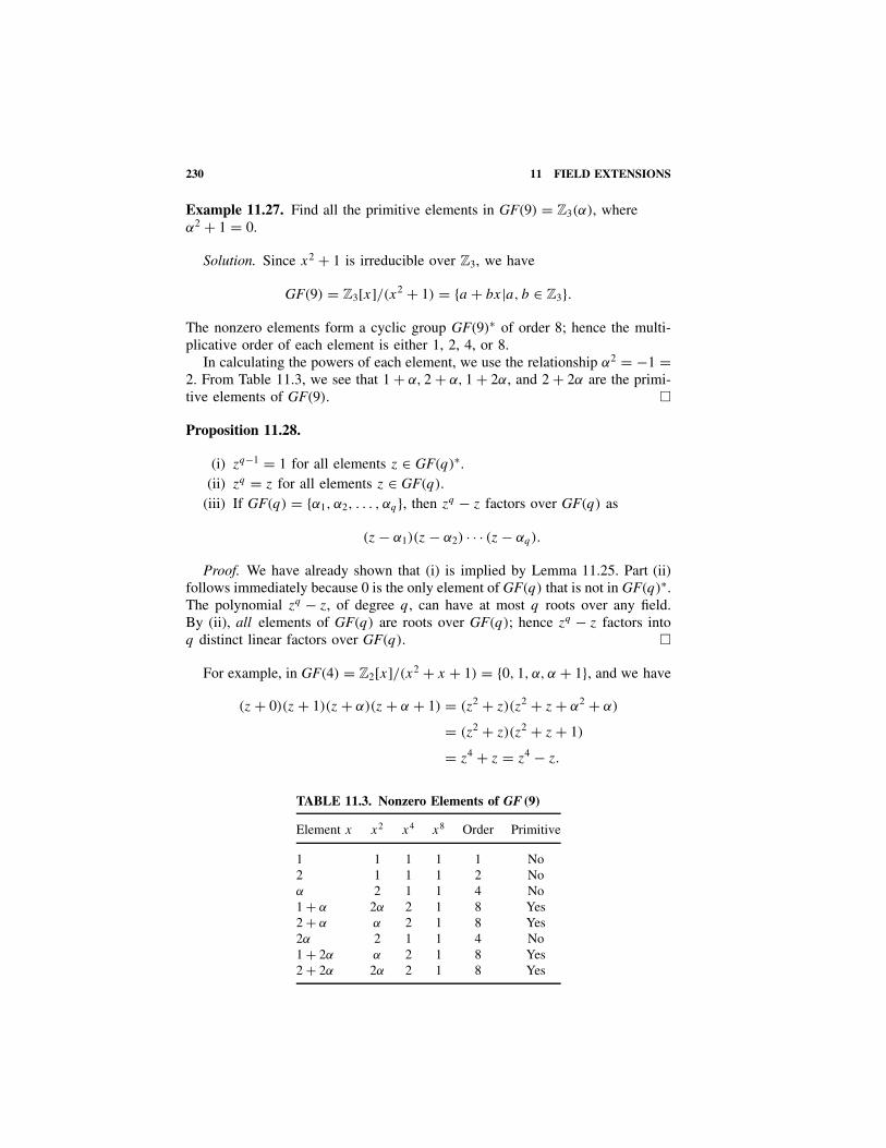
230 11 FIELD EXTENSIONS
Example 11.27. Find all the primitive elements in GF(9) = Z3(α), whereα2 + 1 = 0.
Solution. Since x2 + 1 is irreducible over Z3, we have
GF(9) = Z3[x]/(x2 + 1) = {a + bx|a, b ∈ Z3}.The nonzero elements form a cyclic group GF(9)∗ of order 8; hence the multi-plicative order of each element is either 1, 2, 4, or 8.
In calculating the powers of each element, we use the relationship α2 = −1 =2. From Table 11.3, we see that 1 + α, 2 + α, 1 + 2α, and 2 + 2α are the primi-tive elements of GF(9). �
Proposition 11.28.
(i) zq−1 = 1 for all elements z ∈ GF(q)∗.(ii) zq = z for all elements z ∈ GF(q).
(iii) If GF(q) = {α1, α2, . . . , αq}, then zq − z factors over GF(q) as
(z − α1)(z − α2) · · · (z − αq).
Proof. We have already shown that (i) is implied by Lemma 11.25. Part (ii)follows immediately because 0 is the only element of GF(q) that is not in GF(q)∗.The polynomial zq − z, of degree q, can have at most q roots over any field.By (ii), all elements of GF(q) are roots over GF(q); hence zq − z factors intoq distinct linear factors over GF(q). �
For example, in GF(4) = Z2[x]/(x2 + x + 1) = {0, 1, α, α + 1}, and we have
(z + 0)(z + 1)(z + α)(z + α + 1) = (z2 + z)(z2 + z + α2 + α)
= (z2 + z)(z2 + z + 1)
= z4 + z = z4 − z.
TABLE 11.3. Nonzero Elements of GF (9)
Element x x2 x4 x8 Order Primitive
1 1 1 1 1 No2 1 1 1 2 Noα 2 1 1 4 No1 + α 2α 2 1 8 Yes2 + α α 2 1 8 Yes2α 2 1 1 4 No1 + 2α α 2 1 8 Yes2 + 2α 2α 2 1 8 Yes

PRIMITIVE ELEMENTS 231
An irreducible polynomial g(x), of degree m over Zp, is called a primitivepolynomial if g(x)|(xk − 1) for k = pm − 1 and for no smaller k.
Proposition 11.29. The irreducible polynomial g(x) ∈ Zp[x] is primitive if andonly if x is a primitive element in Zp[x]/(g(x)) = GF(pm).
Proof. The following statements are equivalent:
(i) x is a primitive element in GF(pm) = Zp[x]/(g(x)).(ii) xk = 1 in GF(pm) for k = pm − 1 and for no smaller k.
(iii) xk − 1 ≡ 0 mod g(x) for k = pm − 1 and for no smaller k.(iv) g(x)|(xk − 1) for k = pm − 1 and for no smaller k. �
For example, x2 + x + 1 is primitive in Z2[x]. From Example 11.27, we seethat x2 + 1 is not primitive in Z3[x]. However, 1 + α and 1 + 2α = 1 − α areprimitive elements, and they are roots of the polynomial
(x − 1 − α)(x − 1 + α) = (x − 1)2 − α2 = x2 + x + 2 ∈ Z3[x].
Hence x2 + x + 2 is a primitive polynomial in Z3[x]. Also, x2 + 2x + 2 isanother primitive polynomial in Z3[x] with roots 2 + α and 2 + 2α = 2 − α.
Example 11.30. Let α be a root of the primitive polynomial x4 + x + 1 ∈ Z2[x].Show how the nonzero elements of GF(16) = Z2(α) can be represented by thepowers of α.
Solution. The representation is given in Table 11.4. �
Arithmetic in GF(16) can very easily be performed using Table 11.4. Additionis performed by representing elements as polynomials in α of degree less than 4,whereas multiplication is performed using the representation of nonzero elementsas powers of α. For example,
1 + α + α3
1 + α2 + α3+ α + α2 = α7
α13+ α + α2
= α−6 + α + α2
= α9 + α + α2 since α15 = 1
= α + α3 + α + α2
= α2 + α3.
The concept of primitive polynomials is useful in designing feedback shiftregisters with a long cycle length. Consider the circuit in Figure 11.2, in whichthe square boxes are delays of one unit of time, and the circle with a cross insiderepresents a modulo 2 adder.

232 11 FIELD EXTENSIONS
TABLE 11.4. Representation of GF (16)
Element α0 α1 α2 α3
0 = 0 0 0 0 0α0 = 1 1 0 0 0α1 = α 0 1 0 0α2 = α2 0 0 1 0α3 = α3 0 0 0 1α4 = 1 + α 1 1 0 0α5 = α + α2 0 1 1 0α6 = α2 + α3 0 0 1 1α7 = 1 + α + α3 1 1 0 1α8 = 1 + α2 1 0 1 0α9 = α + α3 0 1 0 1α10 = 1 + α + α2 1 1 1 0α11 = α + α2 + α3 0 1 1 1α12 = 1 + α + α2 + α3 1 1 1 1α13 = 1 + α2 + α3 1 0 1 1α14 = 1 + α3 1 0 0 1
α15 = 1
a0 a1 a2 a3
a4 = 1 + a
Figure 11.2. Feedback shift register.
If the delays are labeled by a representation of the elements of GF(16), asingle shift corresponds to multiplying the element of GF(16) by α. Hence, ifthe contents of the delays are not all zero initially, this shift register will cyclethrough 15 different states before repeating itself. In general, it is possible toconstruct a shift register with n delay units that will cycle through 2n − 1 differentstates before repeating itself. The feedback connections have to be derived from aprimitive polynomial of degree n over Z2. Such feedback shift registers are usefulin designing error-correcting coders and decoders, random number generators,and radar transmitters. See Chapter 14 of this book and, Lidl and Niederreiter [34,Chap. 6], or Stone [22, Chap. 9].

EXERCISES 233
EXERCISES
For Exercises 11.1 to 11.4, write out the addition and multiplication tables forthe fields.
11.1. GF(5). 11.2. GF(7).11.3. GF(9). 11.4. GF(8).
For Exercises 11.5 to 11.10, in each case find, if possible, an irreducible polyno-mial of degree n over F .
11.5. n = 3, F = Z11. 11.6. n = 3, F = Q.11.7. n = 4, F = R. 11.8. n = 3, F = GF(4).11.9. n = 2, F = Q(i). 11.10. n = 5, F = Z3.
For Exercises 11.11 to 11.13, in each case, find a polynomial in F [x] with r asa root.
11.11. r = √2 + √
6, F = Q.11.12. r = π + ei, F = R.11.13. r = 3
√3/
√2, F = Q.
11.14. Show that θ = 2kπ/7 satisfies the equation cos 4θ − cos 3θ = 0 for eachinteger k. Hence find an irreducible polynomial over Q with cos(2π/7)
as a root.11.15. Prove that the algebraic numbers
A = {x ∈ C|x is algebraic over Q}form a subfield of C.
11.16. Assuming the fundamental theorem of algebra, prove that every polyno-mial in A has a root in A.
For Exercises 11.17 to 11.25, Calculate the degrees.
11.17. [Q(3√
7) : Q]. 11.18. [C : Q].
11.19. [Q(i, 3i) : Q]. 11.20. [C : R(√−7)].
11.21. [Z3[x]/(x2 + x + 2) : Z3]. 11.22. [Q(i,√
2) : Q].11.23. [A : Q]. 11.24. [C : A].11.25. [Z3(t) : Z3], where Z3(t) is the field of rational functions in t over Z3.11.26. Prove that x2 − 2 is irreducible over Q(
√3).
For Exercises 11.27 to 11.32, find the inverses of the elements in the given fields.Each field is a finite extension F(α). Express your answers in the form a0 + a1 α +· · · + an−1 αn−1 , where ai ∈ F and [F(α) : F ] = n.
11.27. 1 + 3√
2 in Q(3√
2).11.28. 4
√5 + √
5 in Q(4√
5).11.29. 5 + 6ω in Q(ω), where ω is a complex cube root of 1.
234 11 FIELD EXTENSIONS
11.30. 2 − 3i in Q(i).11.31. α in GF(32) = Z2(α), where α5 + α2 + 1 = 0.11.32. α in GF(27) = Z3(α), where α3 + α2 + 2 = 0.
For Exercises 11.33 to 11.40, find the characteristic of the rings. Which of theseare fields?
11.33. Z2 × Z2. 11.34. Z3 × Z4.11.35. GF(49). 11.36. Z × Z2.
11.37. Q(3√
7). 11.38. M2(Z5).11.39. Q × Z3. 11.40. GF(4)[x].11.41. Let R be any ring and n a positive integer. Prove that In = {na|a ∈ R}
is an ideal of R and that the characteristic of R/In divides n.11.42. Let M be a finite subgroup of the multiplicative group F ∗ of any infinite
field F . Prove that M is cyclic, and give an example to show that F ∗need not be cyclic.
11.43. For what values of m is (Z∗m, ·) cyclic? (This is a difficult problem; see
Exercises 4.55 to 4.62 for other results on Z∗m.)
11.44. Let GF(4) = Z2(α), where α2 + α + 1 = 0. Find an irreducible quadraticin GF(4)[x]. If β is the root of such a polynomial, show that GF(4)(β)
is a Galois field of order 16.11.45. (a) Show that there are (p2 − p)/2 monic irreducible polynomials of
degree 2 over GF(p). (A polynomial is monic if the coefficient ofthe highest power of the variable is 1.)
(b) Prove that there is a field with p2 elements for every prime p.11.46. (a) How many monic irreducible polynomials of degree 3 are there over
GF(p)?(b) Prove that there is a field with p3 elements for every prime p.
11.47. Find an element α such that Q(√
2,√−3) = Q(α).
11.48. Find all primitive elements in GF(16) = Z2(α), where α4 + α +1 = 0.
11.49. Find all the primitive elements in GF(32).
For Exercises 11.50 and 11.51, find a primitive polynomial of degree n over thefield F.
11.50. n = 2, F = Z5. 11.51. n = 3, F = Z2.11.52. Let g(x) be a polynomial of degree m over Zp. If g(x)|(xk − 1) for
k = pm − 1 and for no smaller k, show that g(x) is irreducible over Zp.11.53. Prove that x8 + x ∈ Z2[x] will split into linear factors over GF(8) but not
over any smaller field.11.54. Let f (x) = 2x3 + 5x2 + 7x + 6 ∈ Q[x]. Find a field, smaller than the
complex numbers, in which f (x) splits into linear factors.11.55. If α and β are roots of x3 + x + 1 and x3 + x2 + 1 ∈ Z2[x], respectively,
prove that the Galois fields Z2(α) and Z2(β) are isomorphic.

EXERCISES 235
11.56. (a) If p(x) ∈ Z2[x], prove that [p(x)]2 = p(x2).(b) If β is a root of p(x) ∈ Z2[x], prove that β2l
is a root for all l ∈ N.(c) Let GF(16) = Z2(α) where α4 + α + 1 = 0. Find an irreducible poly-
nomial in Z2[x] with α3 as a root.
For Exercises 11.57 and 11.58, solve the simultaneous linear equations inGF(4 ) = Z2 (α).
11.57. αx + (α + 1)y = α + 1 11.58. (α + 1)x + y = α
x + αy = 1. x + (α + 1)y = α + 1.11.59. Solve the quadratic equation αx2 + (1 + α)x + 1 = 0 over the field
GF(4) = Z2(α).11.60. Let R be any commutative ring of characteristic p, where p is a prime.
(a) Show that (a + b)p = ap + bp for all a, b in R. [Hint: If
(p
r
)
denotes the binomial coefficient, show that
(p
r
)= p
r
(p − 1r − 1
)
whenever 1 � r � p.](b) If σ : R → R is defined by σ(a) = ap for all a ∈ R, show that σ is
a ring morphism.(c) If R = GF(pn) show that σ is an isomorphism of R (called the Frobe-
nius automorphism).11.61. If F is a field and F ∗ is cyclic, show that F is finite.11.62. Design a feedback shift register using six delays that has a cycle length
of 63.11.63. What is the cycle length of the feedback shift register in Figure 11.3?
Figure 11.3
11.64. Design a feedback shift register that has a cycle length of 21.11.65. Describe the output sequence of the feedback shift register in Figure 11.4
when the registers initially contain the elements shown.
1 0 1Output
Figure 11.4
11.66. If a feedback shift register with n delays has a cycle length of 2n − 1,show that the feedback connections must be derived from a primitiveirreducible polynomial of degree n over Z2.

12LATIN SQUARES
Latin squares first arose with parlor games such as the problem of arranging thejacks, queens, kings, and aces of a pack of cards in a 4 × 4 array so that each rowand each column contains one card from each suit and one card from each rank.In 1779, Leonard Euler posed the following famous problem of the 36 officersfrom six ranks and six regiments. He claimed that it was impossible to arrangethese officers on parade in a 6 × 6 square so that each row and each columncontains one officer from each rank and one from each regiment.
Recently, statisticians have found latin squares useful in designing experi-ments, and mathematicians have found close connections between latin squaresand finite geometries.
LATIN SQUARES
Let S be a set with n elements. Then a latin square L = (lij ), of order n basedon S, is an n × n array of the elements of S such that each element appearsexactly once in each row and once in each column.
For example, Table 12.1 illustrates a latin square of order 3 based on {a, b, c}.
Theorem 12.1. The table for any finite group (G, +) of order n is a latin squareof order n based on G.
Proof. We write the operation in G as addition, even though the result stillholds if G is not commutative.
Suppose that two elements in one row are equal. Then xi + xj = xi + xk
for some xi, xj , xk ∈ G. Since G is a group, xi has an inverse (−xi) suchthat (−xi) + xi = 0. Hence (−xi) + (xi + xj ) = (−xi) + (xi + xk), and since theoperation is associative, we have xj = xk. Therefore, an element cannot appeartwice in the same row. Similarly, an element cannot appear twice in the samecolumn, and the table is a latin square. �
Modern Algebra with Applications, Second Edition, by William J. Gilbert and W. Keith NicholsonISBN 0-471-41451-4 Copyright 2004 John Wiley & Sons, Inc.
236

LATIN SQUARES 237
TABLE 12.1. LatinSquare
a b c
c a b
b c a
TABLE 12.2. Latin Squares of Order 4
(0, 0) (0, 1) (1, 0) (1, 1)(0, 1) (0, 0) (1, 1) (1, 0)(1, 0) (1, 1) (0, 0) (0, 1)(1, 1) (1, 0) (0, 1) (0, 0)
c b a d
d a b c
a d c b
b c d a
Given any latin square, we can permute the rows among themselves and alsothe columns among themselves and we still have a latin square. For example, theaddition table for Z2 × Z2 is a latin square of order 4. If we interchange the firstand third columns and replace (0, 0) by a, (0, 1) by b, (1, 0) by c, and (1, 1)by d , we obtain another latin square of order 4 based on {a, b, c, d}. These areillustrated in Table 12.2.
Latin squares are useful in designing statistical experiments because they canshow how an experiment can be arranged so as to reduce the errors withoutmaking the experiment too large or too complicated. See Laywine and Mullen[40] for more complete details.
Suppose that you wanted to compare the yields of three varieties of hybridcorn. You have a rectangular test plot, but you are not sure that the fertility of thesoil is the same everywhere. You could divide up the land into nine rectangularregions and plant the three varieties, a, b, and c, in the form of the latin squarein Table 12.1. Then if one row were more fertile than the others, the latin squarewould reduce the error that this might cause. In fact, if the soil fertility was alinear function of the coordinates of the plot, the latin square arrangement wouldminimize the error.
Of course, the error could be reduced by subdividing the plot into a largenumber of pieces and planting the varieties at random. But this would make itmuch more difficult to sow and harvest.
Example 12.2. A smoking machine is used to test the tar content of four brandsof cigarettes; the machine has four ports so that four cigarettes can be smokedsimultaneously. However, the four ports might not be identical and that mightaffect the measurements of the tar content. Also, if four runs were made on themachine, testing one brand at a time, the humidity could change, thus affectingthe results.
Show how to reduce the errors due to the different ports and the different runsby using a latin square to design the experiment.

238 12 LATIN SQUARES
TABLE 12.3. Design of theSmoking Experiment
Ports
1 2 3 4↓ ↓ ↓ ↓
1 → c b a d
Runs 2 → d a b c
3 → a d c b
4 → b c d a
TABLE 12.4
A B C D EB A E C DC D A E BD E B A CE C D B A
TABLE 12.5
+ ..p ..q..
.
.r A B
.s B A
.
.
Solution. If a, b, c, d are the four brands, we can use one of the latin squaresof order 4 that we have constructed. Table 12.3 illustrates which brand shouldbe tested at each port during each of the four runs. �
Not all latin squares can be obtained from a group table, even if we allowpermutations of the rows and columns.
Example 12.3. Show that the latin square illustrated in Table 12.4 cannot beobtained from a group table.
Solution. By Corollary 4.11, all groups of order 5 are cyclic and are isomor-phic to (Z5, +). Suppose that the latin square in Table 12.4 could be obtainedfrom the addition table of Z5. Since permutations are reversible, it follows that therows and columns of this square could be permuted to obtain the table of Z5. Thefour elements in the left-hand top corner would be taken into four elements form-ing a rectangle in Z5, as shown in Table 12.5. Then we would have p + r = A,q + r = B, p + s = B, and q + s = A for some p, q, r, s ∈ Z5, where p �= q
and r �= s. Hence p + r = A = q + s and q + r = B = p + s. Adding, we havep + q + 2r = p + q + 2s and 2r = 2s. Therefore, 6r = 6s, which implies thatr = s in Z5, which is a contradiction. �
ORTHOGONAL LATIN SQUARES
Suppose that in our cornfield, besides testing the yields of three varieties of corn,we also wanted to test the effects of three fertilizers on the corn. We could do
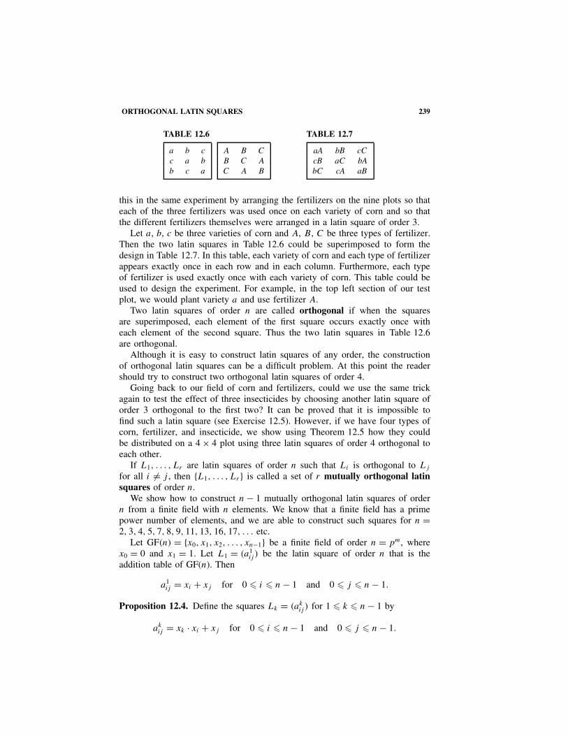
ORTHOGONAL LATIN SQUARES 239
TABLE 12.6
a b c
c a b
b c a
A B C
B C A
C A B
TABLE 12.7
aA bB cCcB aC bAbC cA aB
this in the same experiment by arranging the fertilizers on the nine plots so thateach of the three fertilizers was used once on each variety of corn and so thatthe different fertilizers themselves were arranged in a latin square of order 3.
Let a, b, c be three varieties of corn and A, B, C be three types of fertilizer.Then the two latin squares in Table 12.6 could be superimposed to form thedesign in Table 12.7. In this table, each variety of corn and each type of fertilizerappears exactly once in each row and in each column. Furthermore, each typeof fertilizer is used exactly once with each variety of corn. This table could beused to design the experiment. For example, in the top left section of our testplot, we would plant variety a and use fertilizer A.
Two latin squares of order n are called orthogonal if when the squaresare superimposed, each element of the first square occurs exactly once witheach element of the second square. Thus the two latin squares in Table 12.6are orthogonal.
Although it is easy to construct latin squares of any order, the constructionof orthogonal latin squares can be a difficult problem. At this point the readershould try to construct two orthogonal latin squares of order 4.
Going back to our field of corn and fertilizers, could we use the same trickagain to test the effect of three insecticides by choosing another latin square oforder 3 orthogonal to the first two? It can be proved that it is impossible tofind such a latin square (see Exercise 12.5). However, if we have four types ofcorn, fertilizer, and insecticide, we show using Theorem 12.5 how they couldbe distributed on a 4 × 4 plot using three latin squares of order 4 orthogonal toeach other.
If L1, . . . , Lr are latin squares of order n such that Li is orthogonal to Lj
for all i �= j , then {L1, . . . , Lr} is called a set of r mutually orthogonal latinsquares of order n.
We show how to construct n − 1 mutually orthogonal latin squares of ordern from a finite field with n elements. We know that a finite field has a primepower number of elements, and we are able to construct such squares for n =2, 3, 4, 5, 7, 8, 9, 11, 13, 16, 17, . . . etc.
Let GF(n) = {x0, x1, x2, . . . , xn−1} be a finite field of order n = pm, wherex0 = 0 and x1 = 1. Let L1 = (a1
ij ) be the latin square of order n that is theaddition table of GF(n). Then
a1ij = xi + xj for 0 � i � n − 1 and 0 � j � n − 1.
Proposition 12.4. Define the squares Lk = (akij ) for 1 � k � n − 1 by
akij = xk · xi + xj for 0 � i � n − 1 and 0 � j � n − 1.
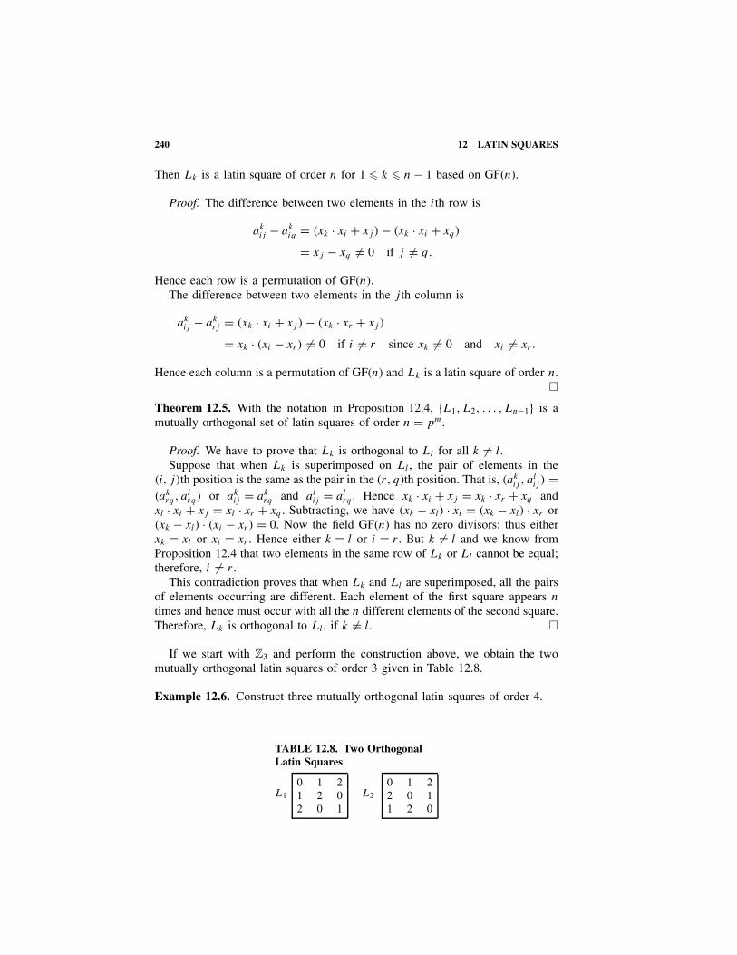
240 12 LATIN SQUARES
Then Lk is a latin square of order n for 1 � k � n − 1 based on GF(n).
Proof. The difference between two elements in the ith row is
akij − ak
iq = (xk · xi + xj ) − (xk · xi + xq)
= xj − xq �= 0 if j �= q.
Hence each row is a permutation of GF(n).The difference between two elements in the j th column is
akij − ak
rj = (xk · xi + xj ) − (xk · xr + xj )
= xk · (xi − xr) �= 0 if i �= r since xk �= 0 and xi �= xr .
Hence each column is a permutation of GF(n) and Lk is a latin square of order n.�
Theorem 12.5. With the notation in Proposition 12.4, {L1, L2, . . . , Ln−1} is amutually orthogonal set of latin squares of order n = pm.
Proof. We have to prove that Lk is orthogonal to Ll for all k �= l.Suppose that when Lk is superimposed on Ll , the pair of elements in the
(i, j)th position is the same as the pair in the (r , q)th position. That is, (akij , a
lij ) =
(akrq , a
lrq) or ak
ij = akrq and al
ij = alrq . Hence xk · xi + xj = xk · xr + xq and
xl · xi + xj = xl · xr + xq . Subtracting, we have (xk − xl) · xi = (xk − xl) · xr or(xk − xl) · (xi − xr) = 0. Now the field GF(n) has no zero divisors; thus eitherxk = xl or xi = xr . Hence either k = l or i = r . But k �= l and we know fromProposition 12.4 that two elements in the same row of Lk or Ll cannot be equal;therefore, i �= r .
This contradiction proves that when Lk and Ll are superimposed, all the pairsof elements occurring are different. Each element of the first square appears n
times and hence must occur with all the n different elements of the second square.Therefore, Lk is orthogonal to Ll , if k �= l. �
If we start with Z3 and perform the construction above, we obtain the twomutually orthogonal latin squares of order 3 given in Table 12.8.
Example 12.6. Construct three mutually orthogonal latin squares of order 4.
TABLE 12.8. Two OrthogonalLatin Squares
L1
0 1 21 2 02 0 1
L2
0 1 22 0 11 2 0

ORTHOGONAL LATIN SQUARES 241
TABLE 12.9. Three Mutually Orthogonal Latin Squares of Order 4
L1
0 1 α α2
1 0 α2 α
α α2 0 1α2 α 1 0
L2
0 1 α α2
α α2 0 1α2 α 1 01 0 α2 α
L3
0 1 α α2
α2 α 1 01 0 α2 α
α α2 0 1
TABLE 12.10. Superimposed LatinSquares
aaa bbb ccc dddbcd adc dab cbacdb dca abd bacdbc cad bda acb
TABLE 12.11. Sixteen Court Cards
A♠ K♦ Q♥ J♣Q♣ J♥ A♦ K♠J♦ Q♠ K♣ A♥K♥ A♣ J♠ Q♦
Solution. Apply the method given in Proposition 12.4 to the Galois fieldGF(4) = Z2(α) = {0, 1, α, α2}, where α2 = α + 1.
L1 is simply the addition table for GF(4). From the way the square Lk wasconstructed in Proposition 12.4, we see that its rows are a permutation of therows of L1. Hence L2 can be obtained by multiplying the first column of L1 byα and then permuting the rows of L1 so that they start with the correct element.L3 is also obtained by permuting the rows of L1 so that the first column is α2
times the first column of L1. These are illustrated in Table 12.9. �
If we write a for 0, b for 1, c for α, and d for α2, and superimpose the threelatin squares, we obtain Table 12.10. Example 12.6 also allows us to solve theparlor game of laying out the 16 cards that was mentioned at the beginning of thechapter. One solution, using the squares L2 and L3 in Table 12.9, is illustratedin Table 12.11.
Example 12.7. A drug company wishes to produce a new cold remedy by com-bining a decongestant, an antihistamine, and a pain reliever. It plans to test variouscombinations of three decongestants, three antihistamines, and three pain reliev-ers on four groups of subjects each day from Monday to Thursday. Furthermore,each type of ingredient should also be compared with a placebo. Design this testso as to reduce the effects due to differences between the subject groups and thedifferent days.
Solution. We can use the three mutually orthogonal latin squares constructedin Example 12.6 to design this experiment—see Table 12.9.
Make up the drugs given to each group using Table 12.12. The letter in thefirst position refers to the decongestant, the second to the antihistamine, and thethird to the pain reliever. The letter a refers to a placebo, and b, c, and d referto the three different types of ingredients. �

242 12 LATIN SQUARES
TABLE 12.12. Testing Three DifferentDrugs
Mon. Tues. Wed. Thurs.
A aaa bbb ccc dddSubject B bcd adc dab cbaGroup C cdb dca abd bac
D dbc cad bda acb
We recognize Euler’s problem of the 36 officers on parade mentioned at thebeginning of the chapter as the problem of constructing two orthogonal latinsquares of order 6. Euler not only conjectured that this problem was impossibleto solve, but he also conjectured that it was impossible to find two orthogonallatin squares of order n, whenever n ≡ 2 mod 4.
Theorem 12.5 cannot be used to construct two such squares with order congruentto 2 modulo 4 because the only prime power of this form is 2, and then the theoremonly gives one latin square. In 1899, G. Tarry, by exhaustive enumeration, provedthat the problem of the 36 officers was insoluble. However, in 1959, Euler’s generalconjecture was shown to be false, and in fact, Bose, Shrikhande, and Parker provedthat there exist at least two orthogonal latin squares of order n, for any n > 6.Hence Proposition 12.4 is by no means the only way of constructing orthogonallatin squares. Laywine and Mullen [40] give a comprehensive survey of all theknown results on latin squares up to the time of the book’s publication in 1998.
FINITE GEOMETRIES
The construction in Theorem 12.5 of n − 1 mutually orthogonal latin squares oforder n, when n is a prime power, was first discovered by the American mathe-matician E. H. Moore in 1896, and was rediscovered by the Indian mathematicalstatistician R. C. Bose in 1938. (See Section 2.2 of Laywine and Mullin [40].)Bose also showed that there is a very close connection between orthogonal latinsquares and geometries with a finite number of points and lines. These geometriesare called affine planes.
An affine plane consists of a set, P , of points, together with a set, L, ofsubsets of P called lines. The points and lines must satisfy the following inci-dence axioms.
(i) Any two distinct points lie on exactly one line.(ii) For each line l and point x not on l, there exists a unique line m containing
x and not meeting l.(iii) There exist three points not lying on a line.
We can define an equivalence relation of parallelism, / /, on the set of lines L,by defining l//m if l = m or l and m contain no common point. Axiom (ii) thenstates that through each point there is a unique line parallel to any other line. The

FINITE GEOMETRIES 243
points and lines in the euclidean plane R2 form such a geometry with an infinitenumber of points.
If the geometry has only a finite number of points, it can be shown that thereexists an integer n such that the geometry contains n2 points and n2 + n lines,and that each line contains n points, while each point lies on n + 1 lines. Such afinite geometry is called an affine plane of order n. In an affine plane of ordern there are n + 1 parallelism classes (see Exercises 12.12 and 12.13).
Figure 12.1 shows an affine plane of order 2 in which P = {a, b, c, d} andL = {{a, b}, {c, d}, {a, c}, {b, c}, {b, d}, {a, d}}.
Bose showed that an affine plane of order n produces a complete set of n − 1mutually orthogonal latin squares of order n, and conversely, that each set ofn − 1 mutually orthogonal latin squares of order n defines an affine plane oforder n.
Theorem 12.8. There exists an affine plane of order n if and only if there existn − 1 mutually orthogonal latin squares of order n.
Proof. Suppose that there exists an affine plane of order n. We coordinatizethe points as follows. Take any line and label the n points as 0, 1, 2, . . . , n − 1.This is called the x-axis, and the point labeled 0 is called the origin. Chooseany other line through the origin and label the n points 0, 1, 2, . . . , n − 1 with0 at the origin. This line is called the y-axis. A point of the plane is said tohave coordinates (a, b) if the unique lines through the point parallel to the y andx-axes meet the axes in points labeled a and b, respectively. This is illustratedin Figure 12.2.
a b
c d
Figure 12.1. Affine plane with four points.
n − 1
b (a, b)
a n − 1
x
y
1
10
Figure 12.2. Coordinates in an affine plane.

244 12 LATIN SQUARES
There are n2 ordered pairs (a, b) corresponding to the n2 points of the plane.These points also correspond to the n2 cells of an n × n square where (a, b)refers to the cell in the ath row and bth column. We fill these cells with numbersin n − 1 different ways to produce n − 1 mutually orthogonal latin squares oforder n.
Consider any complete set of parallel lines that are not parallel to either axis.Label the n parallel lines 0, 1, 2, . . . , n − 1 in any manner. Through each point,there is exactly one of these lines. In the cell (a, b) place the number of theunique line on which the point (a, b) is found. The numbers in these cells forma latin square of order n on {0, 1, . . . , n − 1}. No two numbers in the same rowcan be the same, because there is only one line through two points in the samerow, namely, the line parallel to the x-axis. Hence each number appears exactlyonce in each row and, similarly, once in each column.
There are n − 1 sets of parallelism classes that are not parallel to the axes; eachof these gives rise to a latin square. These n − 1 squares are mutually orthogonalbecause each line of one parallel system meets all n of the lines of any othersystem. Hence, when two squares are superimposed, each number of one squareoccurs once with each number of the second square.
Conversely, suppose that there exists a set of n − 1 mutually orthogonal latinsquares of order n. We can relabel the elements, if necessary, so that these squaresare based on S = {0, 1, 2, . . . , n − 1}. We define an affine plane with S2 as theset of points. A set of n points is said to lie on a line if there is a latin squarewith the same number in each of the n cells corresponding to these points, or ifthe n points all have one coordinate the same. It is straightforward to check thatthis is an affine plane of order n. �
Corollary 12.9. There exists an affine plane of order n whenever n is the powerof a prime.
Proof. This follows from Theorem 12.5. �
The only known affine planes have prime power order. Because of the impos-sibility of solving Euler’s officer problem, there are no orthogonal latin squaresof order 6, and hence there is no affine plane of order 6. In 1988, by means ofa massive computer search, Lam, Thiel, and Swiercz showed that there was noaffine plane of order 10. See Lam [39] for the story behind this two-decade search.By Theorem 12.8, there cannot exist nine mutually orthogonal latin squares oforder 10. However, two mutually orthogonal latin squares of order 10 have beenfound, but not three such squares. Computers have also been used to search formany sets of mutually orthogonal latin squares of low order. See Chapter 2 ofLaywine and Mullen [40] for further results on mutually orthogonal latin squares.
By the method of Theorem 12.8, we can construct an affine plane of order n
from the Galois field GF(n) whenever n is a prime power. The set of points is
P = GF(n)2 = {(x, y)|x, y ∈ GF(n)}.

MAGIC SQUARES 245
(0, a2) (1, a2) (a, a2) (a2, a2)
(a2, a)
(a2, 1)
(a2, 0)
(0, a)
(0, 1)
(0, 0) (1, 0) (a, 0)
(a, 1)
(a, a)(1, a)
(1, 1)
Figure 12.3. Affine plane of order 4 with the points of the line y = αx + α2 enlarged.
It follows from Proposition 12.4 that a line consists of points satisfying a linearequation in x and y with coefficients in GF(n). The slope of a line is defined inthe usual way and is an element of GF(n) or is infinite. Two lines are parallel ifand only if they have the same slope.
For example, if GF(4) = Z2(α) = {0, 1, α, α2}, the 16 points of the affineplane of order 4 are shown in Figure 12.3. The horizontal lines are of the form
y = constant
and have slope 0, whereas the vertical lines are of the form
x = constant
and have infinite slope. The line
y = αx + α2
has slope α and contains the points (0, α2), (1, 1), (α, 0) and (α2, α). This lineis parallel to the lines y = αx, y = αx + 1, and y = αx + α.
Given an affine plane of order n, it is possible to construct a projective planeof order n by adding a “line at infinity” containing n + 1 points correspondingto each parallelism class, so that parallel lines intersect on the line at infinity.The projective plane of order n has n2 + n + 1 points and n2 + n + 1 lines.Furthermore, any projective plane gives rise to an affine plane by taking one lineto be the line at infinity. Hence the existence of a projective plane of order n isequivalent to the existence of an affine plane of the same order.
MAGIC SQUARES
Magic squares have been known for thousands of years, and in times whenparticular numbers were associated with mystical ideas, it was natural that a

246 12 LATIN SQUARES
Figure 12.4. “Melancholia,” an engraving by Albrecht Durer. In the upper right there is a magicsquare of order 4 with the date of the engraving, 1514, in the middle of the bottom row. [Courtesyof Staatliche Museen Kupferstichkabinett, photo by Walter Steinkopf.]
square that displays such symmetry should have been deemed to have magicalproperties. Figure 12.4 illustrates an engraving by Durer, made in 1514, thatcontains a magic square. Magic squares have no applications, and this section isincluded for amusement only.
Publisher's Note:Permission to reproduce this imageonline was not granted by thecopyright holder. Readers are kindlyrequested to refer to the printed versionof this article.

MAGIC SQUARES 247
A magic square of order n consists of the integers 1 to n2 arranged in ann × n square array so that the row sums, column sums, and corner diagonal sumsare all the same.
The sum of each row must be n(n2 + 1)/2, which is 1/n times the sum of allthe integers from 1 to n2. For example, in Durer’s magic square of Figure 12.4,the sum of each row, column, and diagonal is 34.
It is an interesting exercise to try to construct such squares. We show how toconstruct some magic squares from certain pairs of orthogonal latin squares. SeeBall et al. [38] and Laywine and Mullen [40] for other methods of constructingmagic squares.
Let K = (kij ) and L = (lij ) be two orthogonal latin squares of order n on theset S = {0, 1, . . . , n − 1}. Superimpose these two squares to form a square M =(mij ) in which the elements of M are numbers in the base n, whose first digit istaken from K and whose second digit is taken from L. That is, mij = n · kij + lij .Since K and L are orthogonal, all possible combinations of two elements fromS occur exactly once in M . In other words, all the numbers from 0 to n2 − 1occur in M .
Now add 1 to every element of M to obtain the square M ′ = m′ij , where
m′ij = mij + 1.
Lemma 12.10. The square M ′ contains all the numbers between 1 and n2 andis row and column magic; that is, the sums of each row and of each column arethe same.
Proof. In any row or column of M , each number from 0 to n − 1 occursexactly once as the first digit and exactly once as the second digit. Hence thesum is
(0 + 1 + · · · + n − 1)n + (0 + 1 + · · · + n − 1)
= (n + 1)(n − 1)n/2 = n(n2 − 1)/2.
Therefore, each row or column sum of M ′ is n(n2 − 1)/2 + n = n(n2 + 1)/2.�
Example 12.11. Construct the square M ′ from the two orthogonal latin squares,K and L, in Table 12.13.
Solution. Table 12.13 illustrates the superimposed square M in base 3 and inbase 10. By adding one to each element, we obtain the magic square M ′. �
Theorem 12.12. If K and L are orthogonal latin squares of order n on theset {0, 1, 2, . . . , n − 1} and the sum of each of the diagonals of K and L isn(n − 1)/2, then the square M ′ derived from K and L is a magic square oforder n.

248 12 LATIN SQUARES
TABLE 12.13. Construction of a MagicSquare of Order 3
1 2 00 1 22 0 1
0 2 12 1 01 0 2
10 22 0102 11 2021 00 12
K L M (in base 3)
3 8 12 4 67 0 5
4 9 23 5 78 1 6
M (in base 10) M ′
Proof. Lemma 12.10 shows that the sum of each row and each column isn(n2 + 1)/2. A similar argument shows that the sum of each diagonal is alson(n2 + 1)/2. �
There are two common ways in which the sum of the diagonal elements ofK and L can equal n(n − 1)/2.
(i) The diagonal is a permutation of {0, 1, . . . , n − 1}.(ii) If n is odd, every diagonal element is (n − 1)/2.
Both these situations occur in the squares K and L of Table 12.13; thus thesquare M ′, which is constructed from these, is a magic square.
Example 12.13. Construct a magic square of order 4 from two orthogonal latinsquares in Table 12.9.
Solution. By replacing 0, 1, α, α2 by 0, 1, 2, 3, in any order, the squaresL2 and L3 in Table 12.9 satisfy the conditions of Theorem 12.12, because the
TABLE 12.14. Construction of a MagicSquare of Order 4
0 1 2 32 3 0 13 2 1 01 0 3 2
3 2 0 11 0 2 32 3 1 00 1 3 2
L′2 L′
3
03 12 20 3121 30 02 1332 23 11 0010 01 33 22
4 7 9 1410 13 3 815 12 6 15 2 16 11
M (in base 4) M ′

EXERCISES 249
diagonal elements are all different. However, L1 will not satisfy the conditionsof Theorem 12.12, whatever substitutions we make. In L2, replace 0, 1, α, α2 by0, 1, 2, 3, respectively, and in L3 replace 0, 1, α, α2 by 3, 2, 0, 1, respectively, toobtain the squares L′
2 and L′3 in Table 12.14. Combine these to obtain the square
M with entries in base 4. Add 1 to each entry and convert to base 10 to obtainthe magic square M ′ in Table 12.14. �
EXERCISES
12.1. Construct a latin square of order 7 on {a, b, c, d, e, f, g}.12.2. Construct four mutually orthogonal latin squares of order 5.
12.3. Construct four mutually orthogonal latin squares of order 8.
12.4. Construct two mutually orthogonal latin squares of order 9.
12.5. Prove that there are at most (n − 1) mutually orthogonal latin squares oforder n. (You can always relabel each square so that the first rows arethe same.)
12.6. Let L = (lij ) be a latin square of order l on {1, 2, . . . , l} and M = (mij )
be a latin square of order m on {1, 2, . . . , m}. Describe how to constructa latin square of order lm on {1, 2, . . . , l} × {1, 2, . . . , m} from L and M .
12.7. Is the latin square of Table 12.15 the multiplication table for a group oforder 6 with identity A?
TABLE 12.15
A B C D E F
B A F E C D
C F B A D E
D C E B F A
E D A F B C
F E D C A B
12.8. A chemical company wants to test a chemical reaction using seven differ-ent levels of catalyst, a, b, c, d , e, f , g. In the manufacturing process, theraw material comes from the previous stage in batches, and the catalystmust be added immediately. If there are seven reactors, A, B, C, D, E,F , G, in which the catalytic reaction can take place, show how to designthe experiment using seven batches of raw material so as to minimize theeffect of the different batches and of the different reactors.
12.9. A supermarket wishes to test the effect of putting cereal on four shelvesat different heights. Show how to design such an experiment lasting fourweeks and using four brands of cereal.

250 12 LATIN SQUARES
12.10. A manufacturer has five types of toothpaste. He would like to test theseon five subjects by giving each subject a different type each week for fiveweeks. Each type of toothpaste is identified by a different color—red,blue, green, white, or purple—and the manufacturer changes the colorcode each week to reduce the psychological effect of the color. Showhow to design this experiment.
12.11. Quality control would like to find the best type of music to play to itsassembly line workers in order to reduce the number of faulty products.As an experiment, a different type of music is played on four days ina week, and on the fifth day no music at all is played. Design such anexperiment to last five weeks that will reduce the effect of the differentdays of the week.
12.12. The relation of parallelism, //, on the set of lines of an affine plane isdefined by l//m if and only if l = m or l ∩ m = Ø. Prove that // is anequivalence relation.
12.13. Let P be the set of points and L be the set of lines of a finite affine plane.(a) Show that the number of points on a line l equals the number of lines
in any parallelism class not containing l.(b) Deduce that all the lines contain the same number of points.(c) If each line contains n points, show that the plane contains n2 points
and n2 + n lines, each point lying on n + 1 lines. Show also that thereare n + 1 parallelism classes.
12.14. Find all the lines in the affine plane of order 3 whose point set is Z23.
Exercises 12.15 to 12.17 refer to the affine plane of order 9 obtained from GF(9 ) =Z3 (α), where α2 + 1 = 0 .
12.15. Find the line through (2α, 1) that is parallel to the line y = αx + 2 + α.12.16. Find the point of intersection of the lines y = x + α and y = (α + 1)x +
2α.12.17. Find the equation of the line through (0, 2α) and (2, α + 1).12.18. Prove that a magic square of order 3 must have 5 at its center.12.19. Prove that 1 cannot be a corner element of a magic square of order 3.12.20. How many different magic squares of order 3 are there?12.21. How many essentially different magic squares of order 3 are there, that
is, magic squares that cannot be obtained from each other by a symmetryof the square?
12.22. Is there a magic square of order 2?12.23. Find two magic squares of order 4 different from the square in
Example 12.18.12.24. Find a magic square of order 5.12.25. Find a magic square of order 8.12.26. Can you construct a magic square with the present year in the last two
squares of the bottom row?

13GEOMETRICALCONSTRUCTIONS
The only geometric instruments used by the ancient Greeks were a straightedgeand a compass. They did not possess reliable graduated rulers or protractors.However, with these two instruments, they could still perform a wide variety ofconstructions; they could divide a line into any number of equal parts, and theycould bisect angles and construct parallel and perpendicular lines. There werethree famous problems that the Greeks could not solve using these methods:(1) duplication of the cube; that is, given one edge of a cube, construct the edgeof a cube whose volume is double that of the given cube; (2) trisection of anygiven angle; and (3) squaring of the circle; that is, given any circle, construct asquare whose area is the same as that of the circle. For centuries, the solutionto these problems eluded mathematicians, despite the fact that large prizes wereoffered for their discovery.
It was not until the nineteenth century that mathematicians suspected and, infact, proved that these constructions were impossible. In the beginning of thatcentury, nonexistence proofs began appearing in algebra; it was proved that thegeneral polynomial equation of degree 5 could not be solved in terms of nth rootsand rational operations. Similar algebraic methods were then applied to thesegeometric problems. The geometric problems could be converted into algebraicproblems by determining which multiples of a given length could be constructedusing only straightedge and compass. Some of the classical constructions areillustrated in Figure 13.1.
CONSTRUCTIBLE NUMBERS
We are interested in those lengths that can be constructed from a given length.For convenience, we choose our unit of length to be the given length. We see
Modern Algebra with Applications, Second Edition, by William J. Gilbert and W. Keith NicholsonISBN 0-471-41451-4 Copyright 2004 John Wiley & Sons, Inc.
251

252 13 GEOMETRICAL CONSTRUCTIONS
Dividing a length r inton equal segments
rn
r
r
r
√2r
Constructing √2 timesa given length r
P
Constructing a line through Pparallel to a line l
P
l
l
Erecting a perpendicularfrom P to a line l
Figure 13.1. Geometrical constructions using straightedge and compass.
that we can divide a length into any number of equal parts, and hence we canconstruct any rational multiple. However, we can do more than this; we canconstruct irrational multiples such as
√2 by using right-angled triangles.
Given any line segment in the plane, choose rectangular coordinates so thatthe line’s end points are (0, 0) and (1, 0). Any point in the plane that can beconstructed from this line segment by using a straightedge and compass is calleda constructible point. A real number is called constructible if it occurs as onecoordinate of a constructible point. Points can be constructed by performing thefollowing allowable operations a finite number of times. We can:
1. Draw a line through two previously constructed points.2. Draw a circle with center at a previously constructed point and with radius
equal to the distance between two previously constructed points.3. Mark the point of intersection of two straight lines.4. Mark the points of intersection of a straight line and a circle.5. Mark the points of intersection of two circles.
Theorem 13.1. The set of constructible numbers, K , is a subfield of R.
Proof. K is a subset of R, so we have to show that it is a field. That is, ifa, b ∈ K , we have to show that a + b, a − b, ab, and if b �= 0, a/b ∈ K .
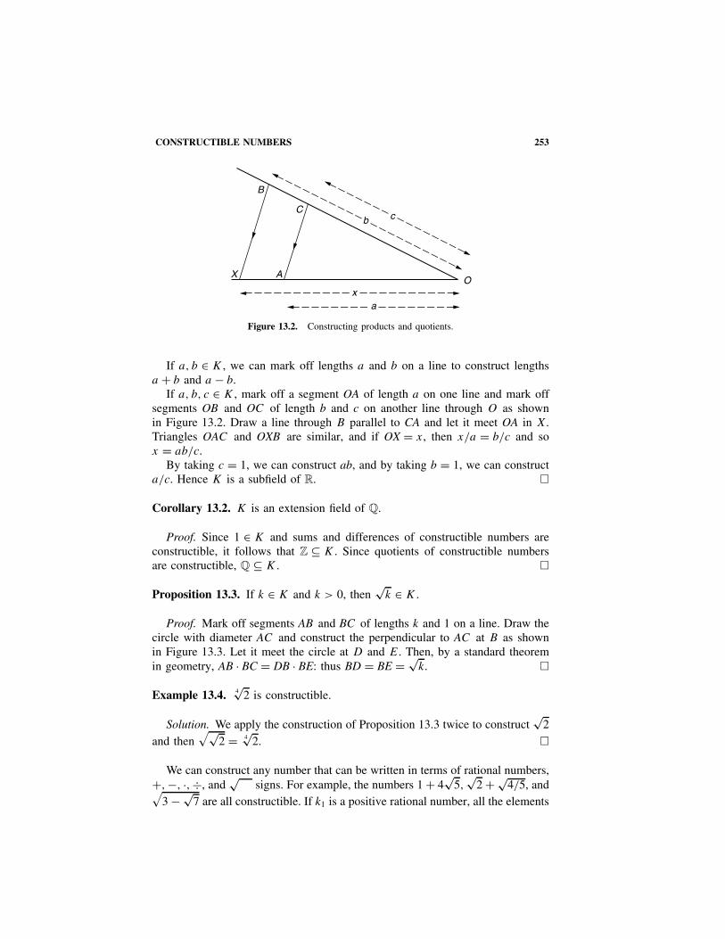
CONSTRUCTIBLE NUMBERS 253
X AO
C
B
b
xa
c
Figure 13.2. Constructing products and quotients.
If a, b ∈ K , we can mark off lengths a and b on a line to construct lengthsa + b and a − b.
If a, b, c ∈ K , mark off a segment OA of length a on one line and mark offsegments OB and OC of length b and c on another line through O as shownin Figure 13.2. Draw a line through B parallel to CA and let it meet OA in X.Triangles OAC and OXB are similar, and if OX = x, then x/a = b/c and sox = ab/c.
By taking c = 1, we can construct ab, and by taking b = 1, we can constructa/c. Hence K is a subfield of R. �
Corollary 13.2. K is an extension field of Q.
Proof. Since 1 ∈ K and sums and differences of constructible numbers areconstructible, it follows that Z ⊆ K . Since quotients of constructible numbersare constructible, Q ⊆ K . �
Proposition 13.3. If k ∈ K and k > 0, then√
k ∈ K .
Proof. Mark off segments AB and BC of lengths k and 1 on a line. Draw thecircle with diameter AC and construct the perpendicular to AC at B as shownin Figure 13.3. Let it meet the circle at D and E. Then, by a standard theoremin geometry, AB · BC = DB · BE: thus BD = BE = √
k. �
Example 13.4. 4√
2 is constructible.
Solution. We apply the construction of Proposition 13.3 twice to construct√
2and then
√√2 = 4
√2. �
We can construct any number that can be written in terms of rational numbers,+, −, ·, ÷, and
√signs. For example, the numbers 1 + 4
√5,
√2 + √
4/5, and√3 − √
7 are all constructible. If k1 is a positive rational number, all the elements

254 13 GEOMETRICAL CONSTRUCTIONS
E
D
CAB
k 1
√k
√k
Figure 13.3. Constructing square roots.
of the extension field K1 = Q(√
k1) are constructible. K1 has degree 1 or 2 overQ depending on whether
√k1 is rational or irrational. If k2 is a positive element
of K1, all the elements of K2 = K1(√
k2) = Q(√
k1,√
k2) are constructible, and[K2 : K1] = 1 or 2, depending on whether or not
√k2 is an element of K1. We
now show that every constructible number lies in a field obtained by repeatingthe extensions above.
Theorem 13.5. The number α is constructible if and only if there exists asequence of real fields K0, K1, . . . , Kn such that α ∈ Kn ⊇ Kn−1 ⊇ · · · ⊇ K0 =Q and [Ki : Ki−1] = 2 for 1 � i � n.
Proof. Suppose that α ∈ Kn ⊇ Kn−1 ⊇ · · · ⊇ K0 = Q, where [Ki : Ki−1] =2. By Proposition 11.16, Ki = Ki−1(
√γi−1) for γi−1 ∈ Ki−1, and since Ki is
real, γi−1 > 0. Therefore, by repeated application of Proposition 13.3, it can beshown that every element of Kn is constructible.
Conversely, suppose that α ∈ K ; thus α appears as the coordinate of a pointconstructible from (0, 0) and (1, 0) by a finite number of the operations 1 to 5preceding Theorem 13.1. We prove the result by induction on m, the number ofconstructible numbers used in reaching α.
Suppose that Xk = {x1, . . . , xk} is a set of numbers that have already beenconstructed, that is, have appeared as coordinates of constructible points. Whenthe next number xk+1 is constructed, we show that [Q(Xk+1) : Q(Xk)] = 1 or 2,where Q(Xk+1) = Q(x1, . . . , xk, xk+1).
We first show that if we perform either operation 1 or 2 using previouslyconstructed numbers in Xk, the coefficients in the equation of the line or circleremain in Q(Xk). If we perform operation 3, the newly constructed numbersremain in Q(Xk), and if we perform operation 4 or 5, the newly constructednumbers are either in Q(Xk) or an extension field of degree 2 over Q(Xk).
Operation 1. The line through (α1, β1) and (α2, β2) is (y − β1)/(β2 − β1) =(x − α1)/(α2 − α1), and if α1, α2, β1, β2 ∈ Xk , the coefficients in the equationof this line lie in Q(Xk).

CONSTRUCTIBLE NUMBERS 255
Operation 2. The circle with center (α1, β1) and radius equal to the distance from(α2, β2) to (α3, β3) is (x − α1)
2 + (y − β1)2 = (α2 − α3)
2 + (β2 − β3)2, and all
the coefficients in this equation lie in Q(Xk).
Operation 3. Let αij , βj ∈ Q(Xk). Then the lines
α11x + α12y = β1
α21x + α22y = β2
meet in the point (x, y), where using Cramer’s rule,
x = det
(β1 α12
β2 α22
) /det
(α11 α12
α21 α22
)
and
y = det
(α11 β1
α21 β2
) /det
(α11 α12
α21 α22
)
as long as they are not parallel. Both of these coordinates are in Q(Xk).
Operation 4. To obtain the points of intersection of a circle and line with coef-ficients in Q(Xk), we eliminate y from the equations to obtain an equation ofthe form
αx2 + βx + γ = 0 where α, β, γ ∈ Q(Xk).
The line and circle intersect if β2 − 4αγ � 0 and the x coordinates of
the intersection points are x = −β ± √β2 − 4αγ
2α, which are in Q(Xk) or
Q(Xk)(√
β2 − 4αγ ). Similarly, the y coordinates are in Q(Xk) or in an extensionfield of degree 2 over Q(Xk).
Operation 5. The intersection of the two circles
x2 + y2 + α1x + β1y + γ1 = 0
x2 + y2 + α2x + β2y + γ2 = 0
is the same as the intersection of one of them with the line
(α1 − α2)x + (β1 − β2)y + (γ1 − γ2) = 0.
This is now the same situation as in operation (4).
Initially, m = 2, X2 = {0, 1}, and Q(X2) = Q. It follows by induction on m,the number of constructible points used, that
α ∈ Q(Xm) ⊇ Q(Xm−1) ⊇ · · · ⊇ Q(X3) ⊇ Q(X2) = Q,

256 13 GEOMETRICAL CONSTRUCTIONS
where [Q(Xk+1) : Q(Xk)] = 1 or 2 for 2 � k � m − 1. Furthermore, each exten-sion field Q(Xk) is a subfield of R because Q and Xk are sets of real numbers. Bydropping each field Q(Xi) that is a trivial extension of Q(Xi−1), it follows that
α ∈ Kn ⊇ Kn−1 ⊇ · · · ⊇ K0 = Q
where [Ki : Ki−1] = 2 for 1 � i � n. �
Corollary 13.6. If α is constructible, then [Q(α) : Q] = 2r for some r � 0.
Proof. If α is constructible, then α ∈ Kn ⊇ Kn−1 ⊇ · · · ⊇ K0 = Q, where Ki
is an extension field of degree 2 over Ki−1. By Theorem 11.6,
[Kn : Q(α)][Q(α) : Q] = [Kn : Q]
= [Kn : Kn−1][Kn−1 : Kn−2] · · · [K1 : Q] = 2n.
Hence [Q(α) : Q]|2n; thus [Q(α) : Q] = 2r for some r � 0. �
Corollary 13.7. If [Q(α) : Q] �= 2r for some r � 0, then α is not constructible.
Corollary 13.6 does not give a sufficient condition for α to be constructible,as shown in Example 13.17 below.
Example 13.8. Can a root of the polynomial x5 + 4x + 2 be constructed usingstraightedge and compass?
Solution. Let α be a root of x5 + 4x + 2. By Eisenstein’s criterion, x5 + 4x +2 is irreducible over Q; thus, by Corollary 11.12, [Q(α) : Q] = 5. Since 5 is nota power of 2, it follows from Corollary 13.7 that α is not constructible. �
Example 13.9. Can a root of the polynomial x4 − 3x2 + 1 be constructed usingstraightedge and compass?
Solution. Solving the equation x4 − 3x2 + 1 = 0, we obtain x2 = (3 ± √5)/2
and x = ±√(3 ± √
5)/2. It follows from Theorem 13.5 that all these roots canbe constructed. �
DUPLICATING A CUBE
Let l be the length of the sides of a given cube so that its volume is l3. A cubewith double the volume will have sides of length 3
√2 l.
Proposition 13.10. 3√
2 is not constructible.

TRISECTING AN ANGLE 257
Proof. 3√
2 is a root of x3 − 2 which, by the rational roots theorem (Theo-rem 9.25), is irreducible over Q. Hence, by Corollary 11.12, [Q(
3√
2) : Q] = 3so, by Corollary 13.7, 3
√2 is not constructible. �
Since we cannot construct a length of 3√
2 l starting with a length l, the ancientproblem of duplicating the cube is insoluble.
TRISECTING AN ANGLE
Certain angles can be trisected using straightedge and compass. For example,π, π/2, 3π/4 can be trisected because π/3, π/6, and π/4 can be constructed.However, we show that not all angles are trisectable by proving that π/3 cannotbe trisected.
If we are given the angle φ, we can drop a perpendicular from a point aunit distance from the angle to construct the lengths cos φ and sin φ, as shownin Figure 13.4. Conversely, if either cos φ or sin φ is constructible, it is pos-sible to construct the angle φ. Hence, if we are given an angle φ, we canconstruct all numbers in the extension field Q(cos φ). Of course, if cos φ ∈ Q,then Q(cos φ) = Q.
We can now consider those numbers that are constructible from Q(cos φ). Thisnotion of constructibility is similar to our previous notion, and similar resultshold, except that the starting field is Q(cos φ) instead of Q.
Theorem 13.11. The angle φ can be trisected if and only if the polynomial4x3 − 3x − cos φ is reducible over Q(cos φ).
Proof. Let θ = φ/3. The angle θ can be constructed from φ if and only ifcos θ can be constructed from cos φ. It follows from De Moivre’s theorem andthe binomial theorem that
cos φ = cos 3θ = 4 cos3 θ − 3 cos θ.
Hence cos θ is a root of f (x) = 4x3 − 3x − cos φ.If f (x) is reducible over Q(cos φ), then cos θ is a root of a polynomial of
degree 1 or 2 over Q(cos φ); thus [Q(cos φ, cos θ) : Q(cos φ)] = 1 or 2. Hence,by Propositions 11.16 and 13.3, cos θ is constructible from Q(cos φ).
cos f
sin f
f
1
Figure 13.4. Constructing sin φ and cos φ from the angle φ.
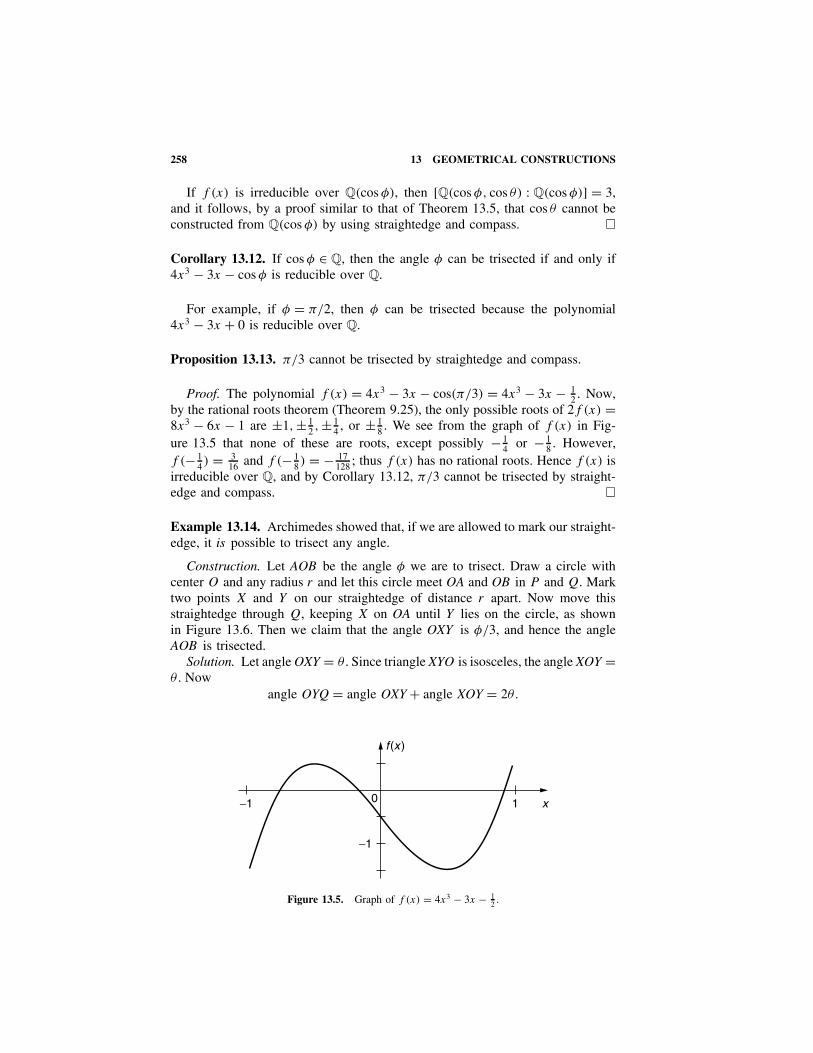
258 13 GEOMETRICAL CONSTRUCTIONS
If f (x) is irreducible over Q(cos φ), then [Q(cos φ, cos θ) : Q(cos φ)] = 3,and it follows, by a proof similar to that of Theorem 13.5, that cos θ cannot beconstructed from Q(cos φ) by using straightedge and compass. �
Corollary 13.12. If cos φ ∈ Q, then the angle φ can be trisected if and only if4x3 − 3x − cos φ is reducible over Q.
For example, if φ = π/2, then φ can be trisected because the polynomial4x3 − 3x + 0 is reducible over Q.
Proposition 13.13. π/3 cannot be trisected by straightedge and compass.
Proof. The polynomial f (x) = 4x3 − 3x − cos(π/3) = 4x3 − 3x − 12 . Now,
by the rational roots theorem (Theorem 9.25), the only possible roots of 2f (x) =8x3 − 6x − 1 are ±1, ± 1
2 , ± 14 , or ± 1
8 . We see from the graph of f (x) in Fig-ure 13.5 that none of these are roots, except possibly − 1
4 or − 18 . However,
f (− 14 ) = 3
16 and f (− 18 ) = − 17
128 ; thus f (x) has no rational roots. Hence f (x) isirreducible over Q, and by Corollary 13.12, π/3 cannot be trisected by straight-edge and compass. �
Example 13.14. Archimedes showed that, if we are allowed to mark our straight-edge, it is possible to trisect any angle.
Construction. Let AOB be the angle φ we are to trisect. Draw a circle withcenter O and any radius r and let this circle meet OA and OB in P and Q. Marktwo points X and Y on our straightedge of distance r apart. Now move thisstraightedge through Q, keeping X on OA until Y lies on the circle, as shownin Figure 13.6. Then we claim that the angle OXY is φ/3, and hence the angleAOB is trisected.
Solution. Let angle OXY = θ . Since triangle XYO is isosceles, the angle XOY =θ . Now
angle OYQ = angle OXY + angle XOY = 2θ.
f (x)
0 1−1
−1
x
Figure 13.5. Graph of f (x) = 4x3 − 3x − 12 .

CONSTRUCTING REGULAR POLYGONS 259
fqq
2qY
rX
2q Q
B
O r P A
Figure 13.6. Trisection of the angle φ using a marked ruler.
Triangle YOQ is isosceles, so angle OQY = 2θ . Also,
φ = angle AOB = angle OXQ + angle OQX = θ + 2θ = 3θ.
Hence θ = φ/3. �
SQUARING THE CIRCLE
Given any circle of radius r , its area is πr2, so that a square with the samearea has sides of length
√π r . We can square the circle if and only if
√π is
constructible.
Proposition 13.15. [Q(√
π) : Q] is infinite, and hence√
π is not constructible.
Proof. The proof of this depends on the fact that π is transcendental overQ; that is, π does not satisfy any polynomial equation with rational coefficients.This was mentioned in Chapter 11, and a proof is given in Stewart [35].
Q(π) is a subfield of Q(√
π) because π = (√
π)2 ∈ Q(√
π). Since π is tran-scendental, π, π2, π3, . . . are linearly independent over Q, and [Q(π) : Q] isinfinite. Therefore,
[Q(√
π) : Q] = [Q(√
π) : Q(π)][Q(π) : Q]
is also infinite. Hence, by Corollary 13.7,√
π is not constructible. �
Hence the circle cannot be squared by straightedge and compass.
CONSTRUCTING REGULAR POLYGONS
Another problem that has been of great interest to mathematicians from the timeof the ancient Greeks is that of constructing a regular n-gon, that is, a regularpolygon with n sides. This is equivalent to constructing the angle 2π/n or the

260 13 GEOMETRICAL CONSTRUCTIONS
number cos(2π/n). The Greeks knew how to construct regular polygons withthree, four, five, and six sides, but were unable to construct a regular 7-gon.
It is well known how to construct an equilateral triangle and a square usingstraightedge and compass. We proved in Example 11.15 that cos(2π/5) =(√
5 − 1)/4; thus a regular pentagon can be constructed. Furthermore, if a regu-lar n-gon is constructible, so is a regular 2n-gon, because angles can be bisectedusing straightedge and compass. Proposition 13.13 shows that π/9 cannot beconstructed; hence 2π/9 and a regular 9-gon cannot be constructed.
In 1796, at the age of 19, Gauss discovered that a regular 17-gon could beconstructed and later showed the only regular n-gons that are constructible are theones for which n = 2kp1 · · · pr , where k � 0 and p1, . . . , pr are distinct primesof the form 22m + 1. Prime numbers of the form 22m + 1 are called Fermatprimes. Pierre de Fermat (1601–1665) conjectured that all numbers of the form22m + 1 are prime. When m = 0, 1, 2, 3, and 4, the numbers are 3, 5, 17, 257, and65,537, respectively, and they are all prime. However, in 1732, Euler discoveredthat 225 + 1 is divisible by 641. Computers have checked many of these numbersfor m > 5, and they have all been composite. In fact, no more Fermat primes areknown today.
A complete proof of Gauss’s result is beyond the scope of this book, since itrequires more group and field theory than we have covered (see Stewart [35]).However, we can prove the following.
Theorem 13.16. If p is a prime for which a regular p-gon is constructible, thenp is a Fermat prime.
Proof. Let ξp = cos(2π/p) + i sin(2π/p), a pth root of unity. If a regularp-gon can be constructed, cos(2π/p) and sin(2π/p) are constructible numbersand [Q(cos(2π/p), sin(2π/p)) : Q] = 2r for some integer r . Hence
[Q(cos(2π/p), sin(2π/p), i) : Q] = 2r+1.
Now Q(ξp) ⊆ Q(cos(2π/p), sin(2π/p), i) and so, by Theorem 11.6,[Q(ξp) : Q] = 2k for some integer k � r + 1.
The pth root of unity, ξp, is a root of the cyclotomic polynomial φ(x) =xp−1 + xp−2 + · · · + x + 1 which, by Example 9.31, is irreducible over Q. Hence[Q(ξp) : Q] = p − 1, and therefore p − 1 = 2k.
The number p = 2k + 1 is a prime only if k = 0 or k is a power of 2. Supposethat k contains an odd factor b > 1 and that k = a · b. Then 2a + 1 divides(2a)b + 1, since x + 1 divides xb + 1 if b is odd. Hence 2ab + 1 cannot be prime.
The case p = 2 gives rise to the degenerate 2-gon. Otherwise, p is a Fermatprime, 22m + 1, for some integer m � 0. �
NONCONSTRUCTIBLE NUMBER OF DEGREE 4
This next example shows that Corollary 13.6 does not give a sufficient conditionfor a number to be constructible.

NONCONSTRUCTIBLE NUMBER OF DEGREE 4 261
Example 13.17. There is a real root ri , of the irreducible polynomial x4 − 4x + 2,that is not constructible, even though [Q(ri) : Q] = 22.
Solution. By Eisenstein’s criterion, x4 − 4x + 2 is irreducible over Q, so that[Q(ri) : Q] = 4 for each root ri . However, we can factor this polynomial intotwo quadratics over R, say
x4 − 4x + 2 = (x2 + ax + b)(x2 + cx + d).
Comparing coefficients, and then using equation (i), we have
(i) 0 = a + c and c = −a
(ii) 0 = b + d + ac and b + d = a2
(iii) −4 = bc + ad and − 4 = a(d − b)
(iv) 2 = bd .
Let t = b + d , so that 16 = a2{(b + d)2 − 4bd} = t (t2 − 8). This number t sat-isfies the equation
(v) t3 − 8t − 16 = 0.
By Theorem 9.25, this equation (v) has no rational roots; thus t3 − 8t − 16 is irre-ducible over Q. We see from Figure 13.7 that the equation does have a real root ρ
between 3 and 4, and the coefficients a, b, c, d can be expressed in terms of ρ.Either a or c is positive. Without loss of generality suppose that c > 0; thus
b + d = t = ρ, a = −c = −√ρ, and d − b = 4/
√ρ. Therefore, we have b =
ρ/2 − 2/√
ρ and d = ρ/2 + 2/√
ρ, and the roots of x2 + ax + b are
−a ± √a2 − 4b
2= 1
2
[√
ρ ±√
−ρ + 8√ρ
],
which are real, since ρ < 4. These are the roots r1 and r2 in Figure 13.8.
−2 2
r
4 t = b + d
t 3 − 8t − 16
0
16
−16
Figure 13.7. Graph of t3 − 8t − 16.

262 13 GEOMETRICAL CONSTRUCTIONS
1 xr2r1
x4 − 4x + 2
0
1
3
2
−1
Figure 13.8. Graph of x4 − 4x + 2.
If both these roots of x4 − 4x + 2 are constructible, then (r1 + r2)2 = ρ is
also constructible. But this is impossible, since ρ is a root of the irreduciblepolynomial t3 − 8t − 16 and [Q(ρ) : Q] = 3.
Hence x4 − 4x + 2 has a real root that is not constructible. �
This example was adapted from the article by Kalmanson [42].
EXERCISES
For Exercises 13.1 to 13.6, which of the numbers are constructible?
13.1. 4√
5 + √2. 13.2. 6
√2.
13.3.2
1 + √7
. 13.4. (1 − 4√
7)3.
13.5. 1 − 5√
27. 13.6. 3√
7 − 5√
2.13.7. Is Q(cos φ) = Q(sin φ) for every angle φ?13.8. If tan φ is constructible, show how to construct the angle φ.13.9. Prove that all the constructible numbers are algebraic over Q.
For the values of cos φ given in Exercises 13.10 to 13.13, determine whether youcan trisect the angle φ by straightedge and compass.
13.10. cos φ = 1/4. 13.11. cos φ = −9/16.
13.12. cos φ = 1/√
2. 13.13. cos φ = √2/8.
13.14. By writing π/15 in terms of π/5 and π/3, show that it is possible totrisect π/5 and also possible to construct a regular 15-gon.
13.15. Can π/7 be trisected?13.16. Construct a regular pentagon using straightedge and compass only.13.17. Prove that cos(2π/7) is a root of 8x3 + 4x2 − 4x − 1 and that 2 cos(2π/7)
is a root of x3 + x2 − 2x − 1. Hence show that a regular septagon is notconstructible.

EXERCISES 263
13.18. If the regular n-gon is constructible and n = qr , show that the regularq-gon is also constructible.
13.19. Let ξ = cos(2π/p2) + i sin(2π/p2). Show that ξ is a root of
f (x) = 1 + xp + x2p + · · · + x(p−1)p.
Prove that f (x) is irreducible over Q by applying Eisenstein’s criterionto f (1 + x).
13.20. Using Exercises 13.18 and 13.19, prove that if a regular n-gon isconstructible, then n = 2kp1 · · · pr where p1, . . . , pr are distinct Fermatprimes.
13.21. Prove that a regular 17-gon is constructible.
For Exercises 13.22 to 13.33, can you construct a root of the polynomials?
13.22. x2 − 7x − 13. 13.23. x4 − 5.13.24. x8 − 16. 13.25. x3 − 10x2 + 2.13.26. x4 + x3 − 12x2 + 7x − 1. 13.27. x5 − 9x3 + 3.13.28. x6 + x3 − 1. 13.29. 3x6 − 8x4 + 1.13.30. 4x4 − x2 + 2x + 1. 13.31. x4 + x − 1.13.32. x48 − 1. 13.33. x4 − 4x3 + 4x2 − 2.
14ERROR-CORRECTING CODES
With the increased use of electronic instrumentation and computers, there is agrowing need for methods of transmitting information quickly and accuratelyover radio and telephone lines and to and from digital storage devices. In fact,CDs and DVDs use error-correcting codes.
Over any transmission line, there is liable to be noise, that is, extraneoussignals that can alter the transmitted information. This is not very noticeable inlistening to the radio or even in reading a telegram, because normal English isabout 20% redundant. However, in transmissions from satellites and in computerlink-ups, the redundancy is usually zero; thus we would like to detect, and possi-bly correct, any errors in the transmitted message. We can do this by putting themessage into a code that will detect and correct most of the errors. (These arenot the sorts of codes useful to a spy. Secret codes are made deliberately hard tobreak, whereas error-correcting codes are designed to be easily decoded.)
One familiar code is the parity check digit that is usually attached to eachnumber inside a computer. A number is written in binary form and a check digitis added that is the sum modulo 2 of the other digits. The sum of the digitsof any number and its check digit is always even unless an error has occurred.This check digit will detect any odd number of errors but not an even numberof errors. This is useful if the probability of two errors occurring in the sameword is very small. When a parity check failure occurs in reading words froma computer memory, the computer automatically rereads the faulty word. If aparity check failure occurs inside the arithmetic unit, the program usually has tobe rerun.
All the codes we construct are obtained by adding a certain number of checkdigits to each block of information. Codes can either be used simply to detecterrors or can be used to correct errors. A code that will detect 2t or fewer errorscan be used to correct t or fewer errors.
Error-detecting codes are used when it is relatively easy to send the originalmessage again, whenever an error is detected. The single parity check code in acomputer is an example of an error-detecting code.
Modern Algebra with Applications, Second Edition, by William J. Gilbert and W. Keith NicholsonISBN 0-471-41451-4 Copyright 2004 John Wiley & Sons, Inc.
264

ERROR-CORRECTING CODES 265
Sometimes it is impossible or too expensive to retransmit the original messagewhen an error is detected. Error-correcting codes then have to be employed.These are used, for example, in transmissions from satellites and space probes(see Figure 14.1). The extra equipment needed to store and retransmit messagesfrom a satellite would add unnecessary weight to the payload. Error-correctingcodes are also used when transmitting data from computer memories to storage
Figure 14.1. In 1969 the Mariners 6 and 7 space probes sent back over 200 close-up photographsof Mars. Each photograph was divided into 658,240 pixels and each pixel was given a brightnesslevel ranging from 1 to 28. Therefore, each photograph required about 5 million bits of information.These bits were encoded, using an error-correcting code, and transmitted at a rate of 16,200 bitsper second back to Earth, where they were received and decoded into photographs. (Courtesy ofNASA/JPL/Caltech.)

266 14 ERROR-CORRECTING CODES
devices. If a message containing an error is stored on a device, it may be weeksbefore it is read and the error detected; by this time the original data mightbe lost.
THE CODING PROBLEM
In most digital computers and many communication systems, information is han-dled in binary form; that is, messages are formed from the symbols 0 and 1.Therefore, in this chapter, we discuss only binary codes. However, most of theresults generalize to codes whose symbols come from any finite field.
We assume that when a message is transmitted over a channel, the probabilityof the digit 1 being changed into 0 is the same as that of 0 being changed into 1.Such channels are called binary symmetric. Figure 14.2 illustrates what mighthappen to a message over a noisy channel.
To transmit a message over a noisy channel, we break up the message intoblocks of k digits and we encode each block by attaching n − k check digits toobtain a code word consisting of n digits, as shown in Figure 14.3. Such a codeis referred to as an (n, k)-code.
The code words can now be transmitted over the noisy channel, and afterbeing received, they can be processed in one of two ways. The code can be usedto detect errors by checking whether or not the received word is a code word.If the received word is a code word, it is assumed to be the transmitted word. If
TransmitterTransmission channel
Encoder
Original message
Receiver
Error detectoror
corrector
Decoded message
noise
1 0 1 1 0 1 0 1 0 0
Figure 14.2. Block diagram for error detection or correction.
k information digits (n, k)–encoder
Message of k digits
k information digitsn − k check digits
Code word of n digits
Figure 14.3. Encoding a block of k digits.
SIMPLE CODES 267
the received word is not a code word, an error must have occurred during trans-mission, and the receiver can request that the word be retransmitted. However,the code could also be used to correct errors. In this case, the decoder choosesthe transmitted code word that is most likely to produce each received word.
Whether a code is used as an error-detecting or error-correcting code dependson each individual situation. More equipment is required to correct errors, andfewer errors can be corrected than could be detected; on the other hand, whena code only detects errors, there is the trouble of stopping the decoding processand requesting retransmission every time an error occurs.
In an (n, k)-code, the original message is k digits long and there are 2k differentpossible messages and hence 2k code words. The received words have n digits;hence there are 2n possible words that could be received, only 2k of which arecode words.
The extra n − k check digits that are added to produce the code word arecalled redundant digits because they carry no new information but only allowthe existing information to be transmitted more accurately. The ratio R = k/n iscalled the code rate or information rate.
For each particular communications channel, it is a major problem to designa code that will transmit useful information as fast as possible and, at the sametime, as reliably as possible.
It was proved by C. E. Shannon in 1948 that each channel has a definitecapacity C, and for any rate R < C, there exist codes of rate R such that theprobability of erroneous decoding is arbitrarily small. In other words, by increas-ing the code length n and keeping the code rate R below the channel capacityC, it is possible to make the probability of erroneous decoding as small as weplease. However, this theory provides no useful method of finding such codes.
For codes to be efficient, they usually have to be very long; they may contain2100 messages and many times that number of possible received words. To beable to encode and decode such long codes effectively, we look at codes thathave a strong algebraic structure.
SIMPLE CODES
We now compare two very simple codes of length 3. The first is the (3, 2)-codethat attaches a single parity check to a message of length 2. The parity checkis the sum modulo 2 of the digits in the message. Hence a received word is acode word if and only if it contains an even number of 1’s. The code words aregiven in Table 14.1. The second code is the (3, 1)-code that repeats a message,consisting of a single digit, three times. Its two code words are illustrated inTable 14.2.
If one error occurs in the (3, 2) parity check code during transmission, say101 is changed to 100, then this would be detected because there would be anodd number of 1’s in the received word. However, this code will not correct anyerrors; the received word 100 is just as likely to have come from 110 or 000 asfrom 101. This code will not detect two errors either. If 101 was the transmitted

268 14 ERROR-CORRECTING CODES
TABLE 14.1. (3, 2)Parity Check Code
Message Code Word
00 00001 10110 11011 011
↑parity check
TABLE 14.2. (3, 1)Repeating Code
Message Code Word
0 0001 111
code word and errors occurred in the first two positions, the received word wouldbe 011, and this would be erroneously decoded as 11.
The decoder first performs a parity check on the received word. If there arean even number of 1’s in the word, the word passes the parity check, and themessage is the last two digits of the word. If there are an odd number of 1’s inthe received work, it fails the parity check, and the decoder registers an error.Examples of this decoding are shown in Table 14.3.
The (3, 1) repeating code can be used as an error-detecting code, and it willdetect one or two transmission errors but, of course, not three errors. This samecode can also be used as an error-correcting code. If the received word containsmore 1’s than 0’s, the decoder assumes that the message is 1; otherwise, itassumes that the message is 0. This will correctly decode messages containingone error, but will erroneously decode messages containing more than one error.Examples of this decoding are shown in Table 14.4.
One useful way to discover the error-detecting and error-correcting capabili-ties of a code is by means of the Hamming distance. The Hamming distancebetween two words u and v of the same length is defined to be the number ofpositions in which they differ. This distance is denoted by d(u, v). For example,d(101, 100) = 1, d(101, 010) = 3, and d(010, 010) = 0.
TABLE 14.3. (3, 2) Parity Check Code Used toDetect Errors
Received Word 101 111 100 000 110
Parity Check Passes Fails Fails Passes Passes
Received Message 01 Error Error 00 10
TABLE 14.4. (3, 1) Repeating Code Usedto Correct Errors
Received Word 111 010 011 000
Decoded Message 1 0 1 0

SIMPLE CODES 269
011
010
000 100
101
111
110
001
Figure 14.4. The code words of the (3,2)parity check code are shown as large dots.
011
010
000 100
101
111
110
001
Figure 14.5. The code words of the (3,1)repeating code are shown as large dots.
The Hamming distance between two words is the number of single errorsneeded to change one word into the other. In an (n, k)-code, the 2n receivedwords can be thought of as placed at the vertices of an n-dimensional cube withunit sides. The Hamming distance between two words is the shortest distancebetween their corresponding vertices along the edges of the n-cube. The 2k codewords form a subset of the 2n vertices, and the code has better error-correctingand error-detecting capabilities the farther apart these code words are. Figure 14.4illustrates the (3,2) parity check code whose code words are at Hamming distance2 apart. Figure 14.5 illustrates the (3,1) repeating code whose code words are atHamming distance 3 apart.
Proposition 14.1. A code will detect all sets of t or fewer errors if and only ifthe minimum Hamming distance between code words is at least t + 1.
Proof. If r errors occur when the code word u is transmitted, the receivedword v is at Hamming distance r from u. These transmission errors will bedetected if and only if v is not another code word. Hence all sets of t or fewererrors in the code word u will be detected if and only if the Hamming distanceof u from all the other code words is at least t + 1. �
Proposition 14.2. A code is capable of correcting all sets of t or fewer errorsif and only if the minimum Hamming distance between code words is at least2t + 1.
Proof. Suppose that the code contains two code words u1 and u2 at Hammingdistance 2t or closer. Then there exists a received word v that differs from u1
and u2 in t or fewer positions. This received word v could have originated fromu1 or u2 with t or fewer errors and hence would not be correctly decoded in boththese situations.
Conversely, any code whose code words are at least 2t + 1 apart is capableof correcting up to t errors. This can be achieved in decoding by choosing thecode word that is closest to each received word. �
Table 14.5 summarizes these results.

270 14 ERROR-CORRECTING CODES
TABLE 14.5. Detection Capabilities of Various Codes
Code
Minimum Distancebetween
Code Words
Number ofErrors
Detectable
Number ofErrors
CorrectableInformation
Rate
(3,2) parity check code 2 1 0 2/3(3,1) repeating code 3 2 1 1/3General (n, k) code d d − 1 � (d − 1)/2 k/n
POLYNOMIAL REPRESENTATION
There are various ways that a word of n binary digits can be represented alge-braically. One convenient way is by means of a polynomial in Z2[x] of degreeless than n. The word a0a1 · · · an−1 can be represented by the polynomial
a0 + a1x + · · · + an−1xn−1 ∈ Z2[x].
We now use this representation to show how codes can be constructed.Let p(x) ∈ Z2[x] be a polynomial of degree n − k. The polynomial code
generated by p(x) is an (n, k)-code whose code words are precisely those poly-nomials, of degree less than n, which are divisible by p(x).
A message of length k is represented by a polynomial m(x), of degree lessthan k. In order that the higher-order coefficients in a code polynomial carry themessage digits, we multiply m(x) by xn−k . This has the effect of shifting themessage n − k places to the right. To encode the message polynomial m(x), wedivide xn−km(x) by p(x) and add the remainder, r(x), to xn−km(x) to form thecode polynomial
v(x) = r(x) + xn−km(x).
This code polynomial is always a multiple of p(x) because, by the divisionalgorithm,
xn−km(x) = q(x) · p(x) + r(x) where deg r(x) < n − k or r(x) = 0;
thusv(x) = r(x) + xn−km(x) = −r(x) + xn−km(x) = q(x) · p(x).
(Remember r(x) = −r(x) in Z2[x].) The polynomial xn−km(x) has zeros in then − k lowest-order terms, whereas the polynomial r(x) is of degree less thann − k; hence the k highest-order coefficients of the code polynomial v(x) arethe message digits, and the n − k lowest-order coefficients are the check digits.These check digits are precisely the coefficients of the remainder r(x).

POLYNOMIAL REPRESENTATION 271
For example, let p(x) = 1 + x2 + x3 + x4 be the generator polynomial of a(7, 3)-code. We encode the message 101 as follows:
message = 1 0 1m(x) = 1 + x2
x4m(x) = x4 + x6
r(x) = 1 + x
v(x) = r(x) + x4m(x) = 1 + x + x4 + x6
code word = 1 1 0 0 1 0 1︸ ︷︷ ︸check digits
︸ ︷︷ ︸message
x2 + x + 1
x4 + x3 + x2 + 0 + 1 x6 +x4
x6+x5+x4 +x2
x5 +x2
x5+x4+x3 +x
x4+x3+x2+x
x4+x3+x2 +1
x+1
The generator polynomial p(x) = a0 + a1x + · · · + an−kxn−k is always cho-
sen so that a0 = 1 and an−k = 1, since this avoids wasting check digits. If a0 = 0,any code polynomial would be divisible by x and the first digit of the code wordwould always be 0; if an−k = 0, the coefficient of xn−k−1 in the code polynomialwould always be 0.
Example 14.3. Write down all the code words for the code generated by thepolynomial p(x) = 1 + x + x3 when the message length k is 3.
Solution. Since deg p(x) = 3, there will be three check digits, and since themessage length k is 3, the code word length n will be 6. The number of messagesis 2k = 8.
x + 1
x3 + 0 + x + 1 x4+x3
x4 +x2+x
x3+x2+x
x3 x+1
x2 +1
Consider the message 110, which is represented by the polynomial m(x) =1 + x. Its check digits are the coefficients of the remainder r(x) = 1 + x2,

272 14 ERROR-CORRECTING CODES
obtained by dividing x3m(x) = x3 + x4 by p(x). Hence the code polynomialis v(x) = r(x) + x3m(x) = 1 + x2 + x3 + x4, and the code word is 101110.Table 14.6 shows all the code words. �
A received message can be checked for errors by testing whether it is divisibleby the generator polynomial p(x). If the remainder is nonzero when the receivedpolynomial u(x) is divided by p(x), an error must have occurred during trans-mission. If the remainder is zero, the received polynomial u(x) is a code word,and either no error has occurred or an undetectable error has occurred.
Example 14.4. If the generator polynomial is p(x) = 1 + x + x3, test whetherthe following received words contain detectable errors: (i) 100011, (ii) 100110,(iii) 101000.
Solution. The received polynomials are 1 + x4 + x5, 1 + x3 + x4, and 1 + x2,respectively. These contain detectable errors if and only if they have nonzeroremainders when divided by p(x) = 1 + x + x3.
x2 + x + 1
x3 + x + 1 x5+x4+ 0+ 0+0+1
x5 +x3+x2
x4+x3+x2 +1x4 +x2+x
x3 +x+1x3 +x+1
0
x + 1
x3 + x + 1 x4+x3+ 0+0+1
x4 +x2+x
x3+x2+x+1x3 +x+1
x2
0
x3 + x + 1 x2+0+1
0
x2 +1
Hence 1 + x4 + x5 is divisible by p(x), but 1 + x3 + x4 and 1 + x2 are not.Therefore, errors have occurred in the latter two words but are unlikely to haveoccurred in the first. �
Table 14.6 lists all the code words for this code. Hence, in Example 14.4 wecan tell at a glance whether a word is a code word simply by noting whether it ison this list. However, in practice, the list of code words is usually so large thatit is easier to calculate the remainder when the received polynomial is dividedby the generator polynomial.

POLYNOMIAL REPRESENTATION 273
TABLE 14.6. (6, 3) Code Generated by 1 + x + x 3
Code Word
Message Check Digits Message Digits
0 0 0 0 0 0 0 0 0
1 0 0 1 1 0 1 0 0
0 1 0 0 1 1 0 1 0
0 0 1 1 1 1 0 0 1
1 1 0 1 0 1 1 1 0
1 0 1 0 0 1 1 0 1
0 1 1 1 0 0 0 1 1
1 1 1 0 1 0 1 1 1
↑ ↑ ↑ ↑ ↑ ↑ ↑ ↑ ↑1 x x2 1 x x2 x3 x4 x5
Furthermore, this remainder can easily be computed using shift registers.Figure 14.6 shows a shift register for dividing by 1 + x + x3. The square boxesrepresent unit delays, and the circle with a cross inside denotes a modulo 2 adder(or exclusive OR gate).
The delays are initially zero, and a polynomial u(x) is fed into this shift registerwith the high-order coefficients first. When all the coefficients of u(x) have beenfed in, the delays contain the remainder of u(x) when divided by 1 + x + x3. Ifthese are all zero, the polynomial u(x) is a code word; otherwise, a detectableerror has occurred. Table 14.7 illustrates this shift register in operation.
The register in Figure 14.6 could be modified to encode messages, becausethe check digits for m(x) are the coefficients of the remainder when x3m(x)
x0 x1 x 2
x3 = 1 + x
u(x)
(high order first)
Figure 14.6. Shift register for dividing by 1 + x + x3.
x1 x 2x0 OR1
2
Encodedmessage
Message
m(x)
v(x)
Figure 14.7. Encoding circuit for a code generated by 1 + x + x3.

274 14 ERROR-CORRECTING CODES
TABLE 14.7. Contents of the Shift Register When1 + x 3 + x 4 Is Divided by 1 + x + x 3
Received Polynomial RegisterWaiting to Enter Contents
Stage Register x0 x1 x2
0 1 0 0 1 1 0 0 0 0 ← register initially zero1 1 0 0 1 1 0 0 02 1 0 0 1 1 0 03 1 0 0 1 1 04 1 0 0 1 15 1 1 1 16 0 0 1 ← remainder is x2
is divided by 1 + x + x3. However, the circuit in Figure 14.7 is more efficientfor encoding. Here the message m(x) is fed simultaneously to the shift registerand the output. While m(x) is being fed in, the switch is in position 1 and theremainder is calculated by the register. Then the switch is changed to position 2,and the check digits are let out to immediately follow the message.
This encoding circuit could also be used for error detection. When u(x) is fedinto the encoding circuit with the switch in position 1, the register calculates theremainder of x3u(x) when divided by p(x). However, u(x) is divisible by p(x)
if and only if x3u(x) is divisible by p(x), assuming that p(x) does not contain afactor x.
How is the generator polynomial chosen so that the code has useful propertieswithout adding too many check digits? We now give some examples.
Proposition 14.5. The polynomial p(x) = 1 + x generates the (n, n − 1) paritycheck code.
Proof. By Proposition 9.33, a polynomial in Z2[x] is divisible by 1 + x if andonly if it contains an even number of nonzero coefficients. Hence the code wordsof a code generated by 1 + x are those words containing an even number of 1’s.The check digit for the message polynomial m(x) is the remainder when xm(x) isdivided by 1 + x. Therefore, by the remainder theorem, Theorem 9.4, the checkdigit is m(1), the parity of the number of 1’s in the message. This code is theparity check code. �
The (3, 1) code that repeats the single message digit three times has codewords 000 and 111, and is generated by the polynomial 1 + x + x2.
We now give one method, using primitive polynomials, of finding a generatorfor a code that will always detect single, double, or triple errors. Furthermore,the degree of the generator polynomial will be as small as possible so that thecheck digits are reduced to a minimum. Recall (see Proposition 11.29) that anirreducible polynomial p(x) of degree m over Z2 is primitive if p(x)|(1 + xk)
for k = 2m − 1 and for no smaller k.

POLYNOMIAL REPRESENTATION 275
Theorem 14.6. If p(x) is a primitive polynomial of degree m, then the(n, n − m)-code generated by p(x) detects all single and double errors whenevern � 2m − 1.
Proof. Let v(x) be a transmitted code word and u(x) = v(x) + e(x) be thereceived word. The polynomial e(x) is called the error polynomial. An error isdetectable if and only if p(x)� |u(x). Since p(x) does divide the code word v(x),an error e(x) will be detectable if and only if p(x)� |e(x).
If a single error occurs, the error polynomial contains a single term, say xi ,where 0 � i < n. Since p(x) is irreducible, it does not have 0 as a root; therefore,p(x)� |xi , and the error xi is detectable.
If a double error occurs, the error polynomial e(x) is of the form xi + xj
where 0 � i < j < n. Hence e(x) = xi(1 + xj−i ), where 0 < j − i < n. Nowp(x)� |xi , and since p(x) is primitive, p(x)� |(1 + xj−i ) if j − i < 2m − 1. Sincep(x) is irreducible, p(x)� |xi(1 + xj−i ) whenever n � 2m − 1, and all doubleerrors are detectable. �
Corollary 14.7. If p1(x) is a primitive polynomial of degree m, the(n, n − m − 1)-code generated by p(x) = (1 + x)p1(x) detects all double errorsand any odd number of errors whenever n � 2m − 1.
Proof. The code words in the code generated by p(x) must be divisible byp1(x) and by (1 + x). The factor (1 + x) has the effect of adding an overallparity check digit to the code. By Proposition 9.33, all the code words have aneven number of terms, and the code will detect any odd number of errors. Sincethe code words are divisible by the primitive polynomial p1(x), the code willdetect all double errors if n � 2m − 1. �
Some primitive polynomials of low degree are given in Table 14.8. Forexample, by adding 11 check digits to a message of length 1012 or less, using thegenerator polynomial (1 + x)(1 + x3 + x10) = 1 + x + x3 + x4 + x10 + x11, wecan detect single, double, triple, and any odd number of errors. Furthermore, the
TABLE 14.8. Short Table of Primitive Polynomialsin Z2[x ]
Primitive Polynomial Degree m 2m − 1
1 + x 1 11 + x + x2 2 31 + x + x3 3 71 + x + x4 4 151 + x2 + x5 5 311 + x + x6 6 631 + x3 + x7 7 1271 + x2 + x3 + x4 + x8 8 2551 + x4 + x9 9 5111 + x3 + x10 10 1023

276 14 ERROR-CORRECTING CODES
encoding and detecting can be done by a small shift register using only 11 delayunits. The number of different messages of length 1012 is 21012, an enormousfigure! When written out in base 10, it would contain 305 digits.
MATRIX REPRESENTATION
Another natural way to represent a word a1a2 . . . an of length n is by the element(a1, a2, . . . , an)
T of the vector space Zn2 = Z2 × Z2 × · · · × Z2 of dimension n
over Z2. We denote the elements of our vector spaces as column vectors, and(a1, a2, . . . , an)
T denotes the transpose of (a1, a2, . . . , an). In an (n, k)-code, the2k possible messages of length k are all the elements of the vector space Zk
2,whereas the 2n possible received words of length n form the vector space Zn
2.An encoder is an injective function
γ : Zk2 → Zn
2
that assigns to each k digit message an n-digit code word.An (n, k)-code is called a linear code if the encoding function is a linear
transformation from Zk2 to Zn
2. Nearly all block codes in use are linear codes, andin particular, all polynomial codes are linear.
Proposition 14.8. Let p(x) be a polynomial of degree n − k that generates an(n, k)-code. Then this code is linear.
Proof. Let γ : Zk2 → Zn
2 be the encoding function defined by the generatorpolynomial p(x). Let m1(x) and m2(x) be two message polynomials of degreeless than k and let m1 and m2 be the same messages considered as vectorsin Zk
2. The code vector γ (mi ) corresponds to the code polynomial vi(x) =ri(x) + xn−kmi(x), where ri(x) is the remainder when xn−kmi(x) is divided byp(x). Now
v1(x) + v2(x) = r1(x) + r2(x) + xn−k[m1(x) + m2(x)],
and r1(x) + r2(x) has degree less than n − k; therefore, r1(x) + r2(x) is theremainder when xn−km1(x) + xn−km2(x) is divided by p(x). Hence v1(x) +v2(x) corresponds to the code vector γ (m1 + m2) and
γ (m1 + m2) = γ (m1) + γ (m2).
Since the only scalars are 0 and 1, this implies that γ is a linear trans-formation. �
Let {e1, e2, . . . , en} be the standard basis of the vector space Zn2, that is, ei
contains a 1 in the ith position and 0’s elsewhere. Let G be the n × k matrix thatrepresents, with respect to the standard basis, the transformation γ : Zk
2 → Zn2,
defined by an (n, k) linear code. This matrix G is called the generator matrixor encoding matrix of the code.
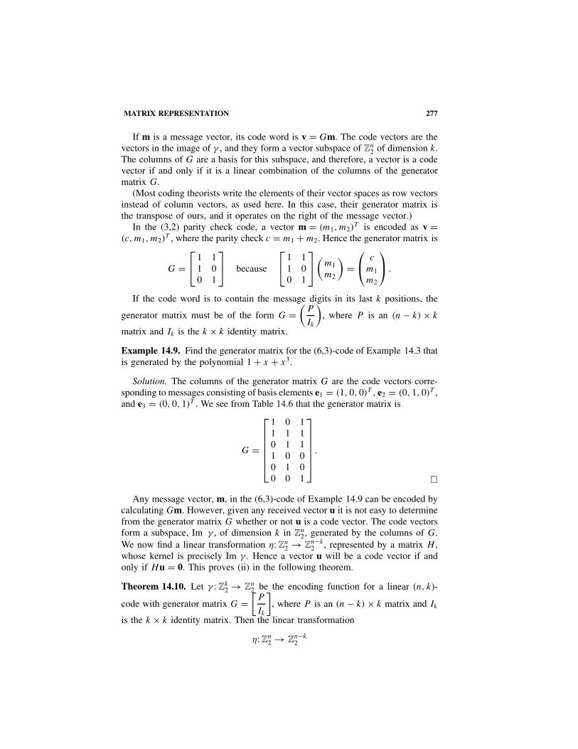
MATRIX REPRESENTATION 277
If m is a message vector, its code word is v = Gm. The code vectors are thevectors in the image of γ , and they form a vector subspace of Zn
2 of dimension k.The columns of G are a basis for this subspace, and therefore, a vector is a codevector if and only if it is a linear combination of the columns of the generatormatrix G.
(Most coding theorists write the elements of their vector spaces as row vectorsinstead of column vectors, as used here. In this case, their generator matrix isthe transpose of ours, and it operates on the right of the message vector.)
In the (3,2) parity check code, a vector m = (m1, m2)T is encoded as v =
(c, m1, m2)T , where the parity check c = m1 + m2. Hence the generator matrix is
G = 1 1
1 00 1
because
1 1
1 00 1
(
m1
m2
)=
c
m1
m2
.
If the code word is to contain the message digits in its last k positions, the
generator matrix must be of the form G =(
P
Ik
), where P is an (n − k) × k
matrix and Ik is the k × k identity matrix.
Example 14.9. Find the generator matrix for the (6,3)-code of Example 14.3 thatis generated by the polynomial 1 + x + x3.
Solution. The columns of the generator matrix G are the code vectors corre-sponding to messages consisting of basis elements e1 = (1, 0, 0)T , e2 = (0, 1, 0)T ,and e3 = (0, 0, 1)T . We see from Table 14.6 that the generator matrix is
G =
1 0 11 1 10 1 11 0 00 1 00 0 1
.
�
Any message vector, m, in the (6,3)-code of Example 14.9 can be encoded bycalculating Gm. However, given any received vector u it is not easy to determinefrom the generator matrix G whether or not u is a code vector. The code vectorsform a subspace, Im γ , of dimension k in Zn
2, generated by the columns of G.We now find a linear transformation η: Zn
2 → Zn−k2 , represented by a matrix H ,
whose kernel is precisely Im γ . Hence a vector u will be a code vector if andonly if Hu = 0. This proves (ii) in the following theorem.
Theorem 14.10. Let γ : Zk2 → Zn
2 be the encoding function for a linear (n, k)-
code with generator matrix G =[
P
Ik
], where P is an (n − k) × k matrix and Ik
is the k × k identity matrix. Then the linear transformation
η: Zn2 → Zn−k
2

278 14 ERROR-CORRECTING CODES
defined by the (n − k) × n matrix H = (In−k|P) has the following properties:
(i) Ker η = Im γ .(ii) A received vector u is a code vector if and only if Hu = 0.
Proof. The composition η Ž γ : Zk2 → Zn−k
2 is the zero transformation because
HG = (In−k|P)
[P
Ik
]= (In−kP + PIk) = P + P = 0
using block multiplication of matrices over the field Z2. Hence Im γ ⊆ Ker η.Since the first n − k columns of H consist of the standard basis vectors in
Zn−k2 , Im η spans Zn−k
2 and contains 2n−k elements. By the morphism theoremfor groups,
|Ker η| = |Zn2|
|Im η| = 2n
2n−k= 2k.
But Im γ also contains 2k elements, and therefore Im γ must equal Ker η. �
The (n − k) × n matrix H in Theorem 14.10 is called the parity check matrixof the (n, k)-code.
The parity check matrix of the (3, 2) parity check code is the 1 × 3 matrixH = (
1 1 1). A received vector u = (u1, u2, u3)
T is a code vector if andonly if
Hu = (1 1 1
) u1
u2
u3
= u1 + u2 + u3 = 0.
The parity check matrix of the (3, 1)-code that repeats the message three
times is the 2 × 3 matrix H =(
1 0 10 1 1
). A received vector u = (u1, u2, u3)
T
is a code vector if and only if Hu = 0, that is, if and only if u1 + u3 = 0 andu2 + u3 = 0. In Z2, this is equivalent to u1 = u2 = u3.
The parity check matrix for the (6, 3)-code of Examples 14.3 and 14.9 is
H = 1 0 0 1 0 1
0 1 0 1 1 10 0 1 0 1 1
.
The received vector u = (u1, . . . , u6)T is a code vector if and only if
u1 + u4 + u6 = 0u2 + u4 + u5 + u6 = 0
u3 + u5 + u6 = 0.
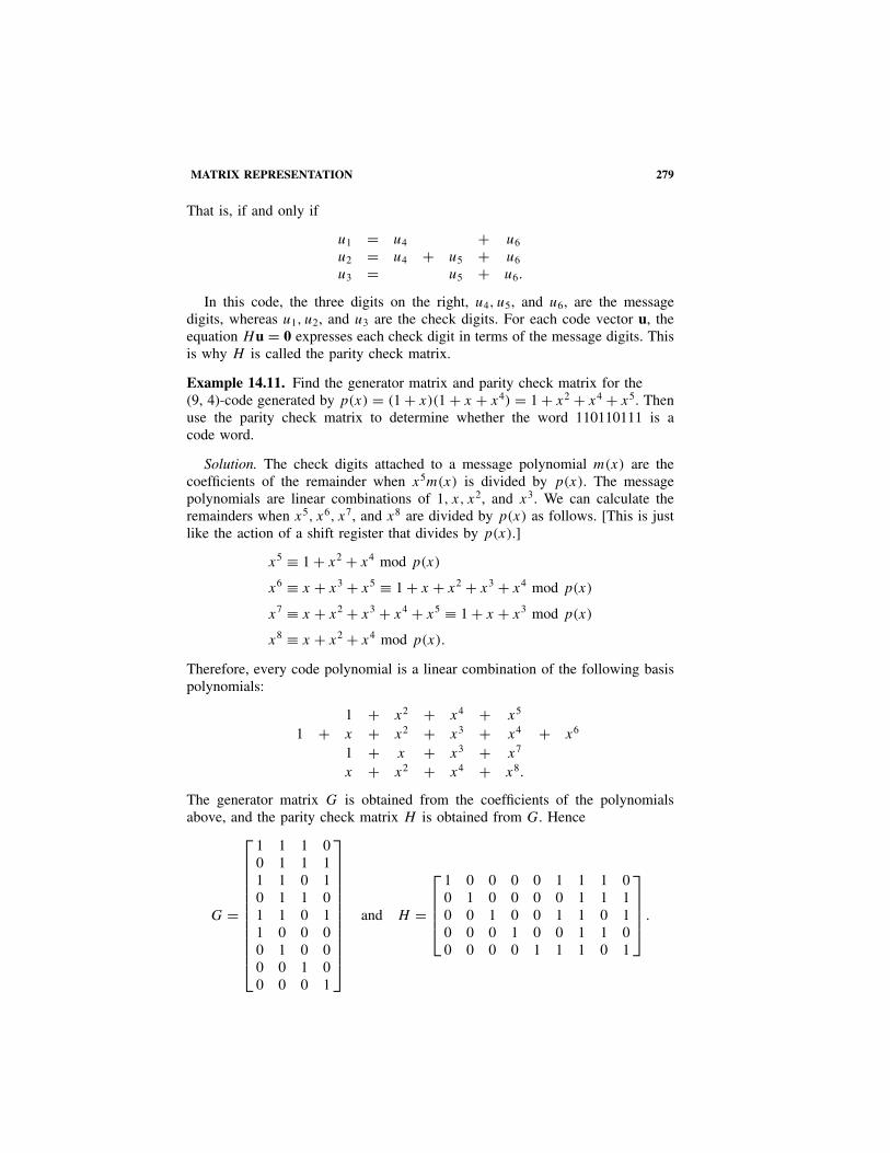
MATRIX REPRESENTATION 279
That is, if and only if
u1 = u4 + u6
u2 = u4 + u5 + u6
u3 = u5 + u6.
In this code, the three digits on the right, u4, u5, and u6, are the messagedigits, whereas u1, u2, and u3 are the check digits. For each code vector u, theequation Hu = 0 expresses each check digit in terms of the message digits. Thisis why H is called the parity check matrix.
Example 14.11. Find the generator matrix and parity check matrix for the(9, 4)-code generated by p(x) = (1 + x)(1 + x + x4) = 1 + x2 + x4 + x5. Thenuse the parity check matrix to determine whether the word 110110111 is acode word.
Solution. The check digits attached to a message polynomial m(x) are thecoefficients of the remainder when x5m(x) is divided by p(x). The messagepolynomials are linear combinations of 1, x, x2, and x3. We can calculate theremainders when x5, x6, x7, and x8 are divided by p(x) as follows. [This is justlike the action of a shift register that divides by p(x).]
x5 ≡ 1 + x2 + x4 mod p(x)
x6 ≡ x + x3 + x5 ≡ 1 + x + x2 + x3 + x4 mod p(x)
x7 ≡ x + x2 + x3 + x4 + x5 ≡ 1 + x + x3 mod p(x)
x8 ≡ x + x2 + x4 mod p(x).
Therefore, every code polynomial is a linear combination of the following basispolynomials:
1 + x2 + x4 + x5
1 + x + x2 + x3 + x4 + x6
1 + x + x3 + x7
x + x2 + x4 + x8.
The generator matrix G is obtained from the coefficients of the polynomialsabove, and the parity check matrix H is obtained from G. Hence
G =
1 1 1 00 1 1 11 1 0 10 1 1 01 1 0 11 0 0 00 1 0 00 0 1 00 0 0 1
and H =
1 0 0 0 0 1 1 1 00 1 0 0 0 0 1 1 10 0 1 0 0 1 1 0 10 0 0 1 0 0 1 1 00 0 0 0 1 1 1 0 1
.

280 14 ERROR-CORRECTING CODES
If the received vector is u = ( 1 1 0 1 1 0 1 1 1 )T ,Hu =( 1 0 0 1 1 )T and hence u is not a code vector. �
Summing up, if G =[
P
Ik
]is the generator matrix of an (n, k)-code, then
H = (In−k|P) is the parity check matrix. We encode a message m by calculatingGm, and we can detect errors in a received vector u by calculating Hu. A linearcode is determined by either giving its generator matrix or by giving its paritycheck matrix.
ERROR CORRECTING AND DECODING
We would like to find an efficient method for correcting errors and decoding. Onecrude method would be to calculate the Hamming distance between a receivedword and each code word. The code word closest to the received word wouldbe assumed to be the most likely transmitted word. However, the magnitude ofthis task becomes enormous as soon as the message length is quite large.
Consider an (n, k) linear code with encoding function γ : Zk2 → Zn
2. Let V =Im γ be the subspace of code vectors. If the code vector v ∈ V is sent through achannel and an error e ∈ Zn
2 occurs during transmission, the received vector willbe u = v + e. The decoder receives the vector u and has to determine the mostlikely transmitted code vector v by finding the most likely error pattern e. Thiserror is e = −v + u = v + u. The decoder does not know what the code vectorv is, but knows that the error e lies in the coset V + u.
The most likely error pattern in each coset of Zn2 by V is called the
coset leader.The coset leader will usually be the element of the coset containing the smallest
number of 1’s. If two or more error patterns are equally likely, one is chosenarbitrarily. In many transmission channels, errors such as those caused by astroke of lightning tend to come in bursts that affect several adjacent digits. Inthese cases, the coset leaders are chosen so that the 1’s in each error pattern arebunched together as much as possible.
The cosets of Zn2 by the subspace V can be characterized by means of the parity
check matrix H . The subspace V is the kernel of the transformation η: Zn2 →
Zn−k2 ; therefore, by the morphism theorem, the set of cosets Zn
2/V is isomorphicto Im η, where the isomorphism sends the coset V + u to η(u) = Hu. Hence thecoset V + u is characterized by the vector Hu.
If H is an (n − k) × n parity check matrix and u ∈ Zn2, then the (n − k)-
dimensional vector Hu is called the syndrome of u. (Syndrome is a medicalterm meaning a pattern of symptoms that characterizes a condition or disease.)
Every element of Zn−k2 is a syndrome; thus there are 2n−k different cosets and
2n−k different syndromes.
Theorem 14.12. Two vectors are in the same coset of Zn2 by V if and only if
they have the same syndrome.

ERROR CORRECTING AND DECODING 281
Proof. If u1, u2 ∈ Zn2, then the following statements are equivalent:
(i) V + u1 = V + u2, (ii) u1 − u2 ∈ V ,(iii) H(u1 − u2) = 0, (iv) Hu1 = Hu2. �
We can decode received words to correct errors by using thefollowing procedure:
1. Calculate the syndrome of the received word.2. Find the coset leader in the coset corresponding to this syndrome.3. Subtract the coset leader from the received word to obtain the most likely
transmitted word.4. Drop the check digits to obtain the most likely message.
For a polynomial code generated by p(x), the syndrome of a received poly-nomial u(x) is the remainder obtained by dividing u(x) by p(x). This is becausethe j th column of H is the remainder obtained by dividing xj−1 by p(x). Hencethe syndrome of elements in a polynomial code can easily be calculated by meansof a shift register that divides by the generator polynomial.
Example 14.13. Write out the cosets and syndromes for the (6,3)-code withparity check matrix
H = 1 0 0 1 0 1
0 1 0 1 1 10 0 1 0 1 1
.
Solution. Each of the rows in Table 14.9 forms a coset with its correspondingsyndrome. The top row is the set of code words.
The element in each coset that is most likely to occur as an error pattern ischosen as coset leader and placed at the front of each row. In the top row 000000is clearly the most likely error pattern to occur. This means that any receivedword in this row is assumed to contain no errors. In each of the next six rows,
TABLE 14.9. Syndromes and All Words of a (6,3) Code
SyndromeCoset
Leader Words
000 000000 110100 011010 111001 101110 001101 100011 010111100 100000 010100 111010 011001 001110 101101 000011 110111010 010000 100100 001010 101001 111110 011101 110011 000111001 001000 111100 010010 110001 100110 000101 101011 011111110 000100 110000 011110 111101 101010 001001 100111 010011011 000010 110110 011000 111011 101100 001111 100001 010101111 000001 110101 011011 111000 101111 001100 100010 010110101 000110 110010 011100 111111 101000 001011 100101 010001

282 14 ERROR-CORRECTING CODES
there is one element containing precisely one nonzero digit; these are chosen ascoset leaders. Any received word in one of these rows is assumed to have oneerror corresponding to the nonzero digit in its coset leader. In the last row, everyword contains at least two nonzero digits. We choose 000110 as coset leader.We could have chosen 101000 or 010001, since these also contain two nonzerodigits; however, if the errors occur in bursts, then 000110 is a more likely errorpattern. Any received word in this last row must contain at least two errors. Indecoding with 000110 as coset leader, we are assuming that the two errors occurin the fourth and fifth digits.
Each word in Table 14.9 can be constructed by adding its coset leader to thecode word at the top of its column. �
A word could be decoded by looking it up in the table and taking the codeword at the top of the column in which it appears. When the code is large, thisdecoding table is enormous, and it would be impossible to store it in a computer.However, in order to decode, all we really need is the parity check matrix tocalculate the syndromes, and the coset leaders corresponding to each syndrome.
Example 14.14. Decode 111001, 011100, 000001, 100011, and 101011 usingTable 14.10, which contains the syndromes and coset leaders. The parity checkmatrix is
H = 1 0 0 1 0 1
0 1 0 1 1 10 0 1 0 1 1
.
Solution. Table 14.11 shows the calculation of the syndromes and the decod-ing of the received words. �
Example 14.15. Calculate the table of coset leaders and syndromes for the (9,4)polynomial code of Example 14.11, which is generated by p(x) = 1 + x2 +x4 + x5. �
TABLE 14.10. Syndromesand Coset Leaders for a(6,3) Code
Syndrome Coset Leader
000 000000100 100000010 010000001 001000110 000100011 000010111 000001101 000110

ERROR CORRECTING AND DECODING 283
TABLE 14.11. Decoding Using Syndromes and Coset Leaders
Word received u 111001 011100 000001 100011 101011Syndrome Hu 000 101 111 000 001Coset leader e 000000 000110 000001 000000 001000Code word u + e 111001 011010 000000 100011 100011Message 001 010 000 011 011
Solution. There is no simple algorithm for finding all the coset leaders. Onemethod of finding them is as follows.
We write down, in Table 14.12, the 25 possible syndromes and try to find theircorresponding coset leaders. We start filling in the table by first entering the errorpatterns, with zero or one errors, next to their syndromes. These will be the mostlikely errors to occur. The error pattern with one error in the j th position is the j thstandard basis vector in Z9
2 and its syndrome is the j th column of the parity checkmatrix H , given in Example 14.11. So, for instance, H(000000001) = 01101, thelast column of H .
The next most likely errors to occur are those with two adjacent errors. Weenter all these in the table. For example,
H(000000011) = H(000000010) + H(000000001)
= 11010 + 01101, the last two columns of H
= 10111.
This still does not fill the table. We now look at each syndrome without acoset leader and find the simplest way the syndrome can be constructed from thecolumns of H . Most of them come from adding two columns, but some have tobe obtained by adding three columns. �
TABLE 14.12. Syndromes and Their Coset Leaders for a (9,4) Code
Syndrome Coset Leader Syndrome Coset Leader Syndrome Coset Leader
00000 000000000 01011 000011100 10110 00011100000001 000010000 01100 011000000 10111 00000001100010 000100000 01101 000000001 11000 11000000000011 000110000 01110 011100000 11001 11001000000100 001000000 01111 000001010 11010 00000001000101 000000110 10000 100000000 11011 00001001000110 001100000 10001 001001000 11100 11100000000111 001110000 10010 000000101 11101 00010010001000 010000000 10011 001101000 11110 00001010001001 010010000 10100 000011000 11111 00000010001010 000001100 10101 000001000

284 14 ERROR-CORRECTING CODES
TABLE 14.13. Decoding Using Syndromes and Coset Leaders
Word received u 100110010 100100101 111101100 000111110Syndrome Hu 01000 00000 10111 10011Coset leader e 010000000 000000000 000000011 001101000Code word u + e 110110010 100100101 111101111 001010110Message 0010 0101 1111 0110
The (9,4)-code in Example 14.15 will, by Corollary 14.7, detect single, dou-ble, and triple errors. Hence it will correct any single error. It will not detect allerrors involving four digits or correct all double errors, because 000000000 and100001110 are two code words of Hamming distance 4 apart. For example, ifthe received word is 100001000, whose syndrome is 00101, Table 14.12 woulddecode this as 100001110 rather than 000000000; both these code words differfrom the received word by a double error.
Example 14.16. Decode 100110010, 100100101, 111101100, and 000111110using the parity check matrix in Example 14.11 and the coset leaders inTable 14.12.
Solution. Table 14.13 illustrates the decoding process. �
BCH CODES
The most powerful class of error-correcting codes known to date werediscovered around 1960 by Hocquenghem and independently by Bose andChaudhuri. For any positive integers m and t , with t < 2m−1, there exists aBose–Chaudhuri–Hocquenghem (BCH) code of length n = 2m − 1 that willcorrect any combination of t or fewer errors. These codes are polynomial codeswith a generator p(x) of degree � mt and have message length at least n − mt .
A t-error-correcting BCH code of length n = 2m − 1 has a generator poly-nomial p(x) that is constructed as follows. Take a primitive element α in theGalois field GF(2m). Let pi(x) ∈ Z2[x] be the irreducible polynomial with αi asa root, and define
p(x) = lcm(p1(x), p2(x), . . . , p2t (x)).
It is clear that α, α2, α3, . . . , α2t are all roots of p(x). By Exercise 11.56,[pi(x)]2 = pi(x
2) and hence α2i is a root of pi(x). Therefore,
p(x) = lcm(p1(x), p3(x), . . . , p2t−1(x)).
Since GF(2m) is a vector space of degree m over Z2, for any β = αi , theelements 1, β, β2, . . . , βm are linearly dependent. Hence β satisfies a polynomialof degree at most m in Z2[x], and the irreducible polynomial pi(x) must also

BCH CODES 285
have degree at most m. Therefore,
deg p(x) � deg p1(x) · deg p3(x) · · · deg p2t−1(x) � mt.
Example 14.17. Find the generator polynomials of the t-error-correcting BCHcodes of length n = 15 for each value of t less than 8.
Solution. Let α be a primitive element of GF (16), where α4 + α + 1 = 0.We repeatedly refer back to the elements of GF (16) given in Table 11.4 whenperforming arithmetic operations in GF(16) = Z2(α).
We first calculate the irreducible polynomials pi(x) that have αi as roots. Weonly need to look at the odd powers of α. The element α itself is the root ofx4 + x + 1. Therefore, p1(x) = x4 + x + 1.
If the polynomial p3(x) contains α3 as a root, it also contains
(α3)2 = α6, (α6)2 = α12, (α12)2 = α24 = α9, and (α9)2 = α18 = α3.
Hence
p3(x) = (x − α3)(x − α6)(x − α12)(x − α9)
= (x2 + (α3 + α6)x + α9)(x2 + (α12 + α9)x + α21)
= (x2 + α2x + α9)(x2 + α8x + α6)
= x4 + (α2 + α8)x3 + (α9 + α10 + α6)x2 + (α17 + α8)x + α15
= x4 + x3 + x2 + x + 1.
The polynomial p5(x) has roots α5, α10, and α20 = α5. Hence
p5(x) = (x − α5)(x − α10)
= x2 + x + 1.
The polynomial p7(x) has roots α7, α14, α28 = α13, α26 = α11, and α22 = α7.Hence
p7(x) = (x − α7)(x − α14)(x − α13)(x − α11)
= (x2 + αx + α6)(x2 + α4x + α9)
= x4 + x3 + 1.
Now every power of α is a root of one of the polynomials p1(x), p3(x), p5(x),or p7(x). For example, p9(x) contains α9 as a root, and therefore, p9(x) = p3(x).
The BCH code that corrects one error is generated by p(x) = p1(x) = x4 +x + 1.
The BCH code that corrects two errors is generated by
p(x) = lcm(p1(x), p3(x)) = (x4 + x + 1)(x4 + x3 + x2 + x + 1).

286 14 ERROR-CORRECTING CODES
This least common multiple is the product because p1(x) and p3(x) are differentirreducible polynomials. Hence p(x) = x8 + x7 + x6 + x4 + 1.
The BCH code that corrects three errors is generated by
p(x) = lcm(p1(x), p3(x), p5(x))
= (x4 + x + 1)(x4 + x3 + x2 + x + 1)(x2 + x + 1)
= x10 + x8 + x5 + x4 + x2 + x + 1.
The BCH code that corrects four errors is generated by
p(x) = lcm(p1(x), p3(x), p5(x), p7(x))
= p1(x) · p3(x) · p5(x) · p7(x)
= x15 + 1
x + 1=
14∑i=0
xi.
This polynomial contains all the elements of GF (16) as roots, except for 0 and 1.Since p9(x) = p3(x), the five-error-correcting BCH code is generated by
p(x) = lcm(p1(x), p3(x), p5(x), p7(x), p9(x))
= (x15 + 1)/(x + 1),
and this is also the generator of the six- and seven-error-correcting BCH codes.These results are summarized in Table 14.14. �
For example, the two-error-correcting BCH code is a (15, 7)-code with gen-erator polynomial x8 + x7 + x6 + x4 + 1. It contains seven message digits andeight check digits.
The seven-error-correcting code generated by (x15 + 1)/(x + 1) has messagelength 1, and the two code words are the sequence of 15 zeros and the sequenceof 15 ones. Each received word can be decoded by majority rule to give the
TABLE 14.14. Construction of t-Error-Correcting BCH Codes of Length 15
t
Roots ofp2t−1(x)
Degree,p2t−1(x) p(x) Degp(x) = 15 − k
MessageLength, k
1 α, α2, α4, α8 4 p1(x) 4 112 α3, α6, α12, α9 4 p1(x)p3(x) 8 73 α5, α10 2 p1(x)p3(x)p5(x) 10 54 α7, α14, α13, α11 4 (x15 + 1)/(x + 1) 14 15 α9, α3, α6, α12 4 (x15 + 1)/(x + 1) 14 16 α11, α7, α14, α13 4 (x15 + 1)/(x + 1) 14 17 α13, α11, α7, α14 4 (x15 + 1)/(x + 1) 14 1
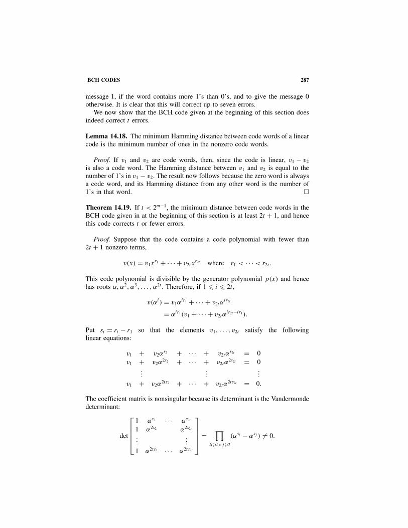
BCH CODES 287
message 1, if the word contains more 1’s than 0’s, and to give the message 0otherwise. It is clear that this will correct up to seven errors.
We now show that the BCH code given at the beginning of this section doesindeed correct t errors.
Lemma 14.18. The minimum Hamming distance between code words of a linearcode is the minimum number of ones in the nonzero code words.
Proof. If v1 and v2 are code words, then, since the code is linear, v1 − v2
is also a code word. The Hamming distance between v1 and v2 is equal to thenumber of 1’s in v1 − v2. The result now follows because the zero word is alwaysa code word, and its Hamming distance from any other word is the number of1’s in that word. �
Theorem 14.19. If t < 2m−1, the minimum distance between code words in theBCH code given in at the beginning of this section is at least 2t + 1, and hencethis code corrects t or fewer errors.
Proof. Suppose that the code contains a code polynomial with fewer than2t + 1 nonzero terms,
v(x) = v1xr1 + · · · + v2t x
r2t where r1 < · · · < r2t .
This code polynomial is divisible by the generator polynomial p(x) and hencehas roots α, α2, α3, . . . , α2t . Therefore, if 1 � i � 2t ,
v(αi) = v1αir1 + · · · + v2tα
ir2t
= αir1(v1 + · · · + v2tαir2t−ir1).
Put si = ri − r1 so that the elements v1, . . . , v2t satisfy the followinglinear equations:
v1 + v2αs2 + · · · + v2tα
s2t = 0v1 + v2α
2s2 + · · · + v2tα2s2t = 0
......
...
v1 + v2α2ts2 + · · · + v2tα
2ts2t = 0.
The coefficient matrix is nonsingular because its determinant is the Vandermondedeterminant:
det
1 αs2 · · · αs2t
1 α2s2 α2s2t
......
1 α2ts2 · · · α2ts2t
=
∏2t�i>j�2
(αsi − αsj ) �= 0.

288 14 ERROR-CORRECTING CODES
This determinant is nonzero because α, α2, . . . , α2t are all different if t < 2m−1.[The expression for the Vandermonde determinant can be verified as follows.When the j th column is subtracted from the ith column, each term containsa factor (αsi − αsj ); hence the determinant contains this factor. Both sides arepolynomials in αs2, . . . , αs2t of the same degree and hence must differ by amultiplicative constant. By looking at the leading diagonal, we see that thisconstant is 1.]
The linear equations above must have the unique solution v1 = v2 = · · · =v2t = 0. Therefore, there are no nonzero code words with fewer than 2t + 1ones, and, by Lemma 14.18 and Proposition 14.2, the code will correct t orfewer errors. �
There is, for example, a BCH (127,92)-code that will correct up to five errors.This code adds 35 check digits to the 92 information digits and hence contains235 syndromes. It would be impossible to store all these syndromes and theircoset leaders in a computer, so decoding has to be done by other methods. Theerrors in BCH codes can be found by algebraic means without listing the tableof syndromes and coset leaders.
In fact, any code with a relatively high information rate must be long andconsequently, to be useful, must possess a simple algebraic decoding algorithm.Further details of the BCH and other codes can be found in Roman [46], Lidland Pilz [10], and Lidl and Niederreiter [34].
EXERCISES
14.1. Which of the following received words contain detectable errors whenusing the (3, 2) parity check code?
110, 010, 001, 111, 101, 000.
14.2. Decode the following words using the (3, 1) repeating code to cor-rect errors:
111, 011, 101, 010, 000, 001.
Which of the words contain detectable errors?14.3. An ancient method of detecting errors when performing the arithmeti-
cal operations of addition, multiplication, and subtraction is the methodknown as casting out nines. For each number occurring in a calcula-tion, a check digit is found by adding together the digits in the numberand casting out any multiples of nine. The original calculation is thenperformed on these check digits instead of on the original numbers. Theanswer obtained, after casting out nines, should equal the check digit ofthe original answer. If not, an error has occurred. For example, checkthe following:
9642 × (425 − 163) = 2526204.

EXERCISES 289
Add the digits of each number; 9 + 6 + 4 + 2 = 21 = 2 × 9 + 3, 4 + 2 +5 = 9 + 2, 1 + 6 + 3 = 9 + 1. Cast out the nines and perform the calcu-lation on these check digits:
3 × (2 − 1) = 3.
Now 3 is the check digit for the answer because 2 + 5 + 2 + 6 +2 + 0 + 4 = 2 × 9 + 3; hence this calculation checks. Why does thismethod work?
14.4. Find the redundancy of the English language. Copy a paragraph from abook leaving out every nth letter, and ask a friend to try to read the para-graph. (Try n = 2, 3, 4, 5, 6. If a passage with every fifth letter missingcan usually be read, the redundancy is at least 1
5 or 20%.)14.5. Each recent book, when published, is given an International Standard
Book Number (ISBN) consisting of ten digits, for example, 0-471-29891-3. The first digit is a code for the language group, the second set of digitsis a code for the publisher, and the third group is the publisher’s numberfor the book. The last digit is one of 0, 1, 2, . . . , 9, X and is a check digit.Have a look at some recent books and discover how this check digit iscalculated. What is the 1 × 10 parity check matrix? How many errorsdoes this code detect? Will it correct any?
14.6. Is 1 + x3 + x4 + x6 + x7 or x + x2 + x3 + x6 a code word in the (8,4)polynomial code generated by p(x) = 1 + x2 + x3 + x4?
14.7. Write down all the code words in the (6,3)-code generated by p(x) =1 + x2 + x3.
14.8. Design a code for messages of length 20, by adding as few check digitsas possible, that will detect single, double, and triple errors. Also give ashift register encoding circuit for your code.
14.9. Decode the following, using the (6,3)-code given in Table 14.9:
000101, 011001, 110000.
14.10. A (7,4) linear code is defined by the equations
u1 = u4 + u5 + u7, u2 = u4 + u6 + u7, u3 = u4 + u5 + u6,
where u4, u5, u6, u7 are the message digits and u1, u2, u3 are the checkdigits. Write down the generator and parity check matrices for this code.Decode the received words 0000111 and 0001111 to correct any errors.
14.11. Find the minimum Hamming distance between the code words of the codewith generator matrix G, where
GT =
0 0 1 0 1 1 0 0 00 1 0 1 0 0 1 0 01 0 1 0 0 0 0 1 00 1 1 0 1 0 0 0 1
.

290 14 ERROR-CORRECTING CODES
Discuss the error-detecting and error-correcting capabilities of this code,and write down the parity check matrix.
14.12. Encode the following messages using the generator matrix of the (9,4)-code of Example 14.11:
1101, 0111, 0000, 1000.
For Exercises 14.13 to 14.15, find the generator and parity check matrices for thepolynomial codes.
14.13. The (4,1)-code generated by 1 + x + x2 + x3.14.14. The (7,3)-code generated by (1 + x)(1 + x + x3).14.15. The (9,4)-code generated by 1 + x2 + x5.14.16. Find the syndromes of all the received words in the (3,2) parity
check code.14.17. Using the parity check matrix in Example 14.14 and the syndromes in
Table 14.10, decode the following words:
101110, 011000, 001011, 111111, 110011.
14.18. Using the parity check matrix in Example 14.11 and the syndromes inTable 14.12, decode the following words:
110110110, 001001101, 111111111, 000000111.
For Exercises 14.19 to 14.22, construct a table of coset leaders and syndromesfor each code.
14.19. The (3,1)-code generated by 1 + x + x2.14.20. The (7,4)-code with parity check matrix
H = 1 0 0 1 1 1 0
0 1 0 1 1 0 10 0 1 1 0 1 1
.
14.21. The (9,4)-code generated by 1 + x2 + x5.14.22. The (7,3)-code generated by (1 + x)(1 + x + x3).14.23. Consider the (63,56)-code generated by (1 + x)(1 + x + x6).
(a) What is the number of digits in the message before coding?(b) What is the number of check digits?(c) How many different syndromes are there?(d) What is the information rate?(e) What sort of errors will it detect?(f) How many errors will it correct?
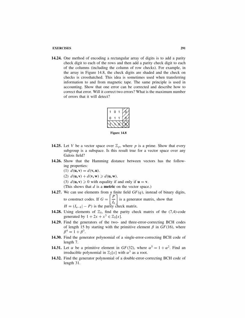
EXERCISES 291
14.24. One method of encoding a rectangular array of digits is to add a paritycheck digit to each of the rows and then add a parity check digit to eachof the columns (including the column of row checks). For example, inthe array in Figure 14.8, the check digits are shaded and the check onchecks is crosshatched. This idea is sometimes used when transferringinformation to and from magnetic tape. The same principle is used inaccounting. Show that one error can be corrected and describe how tocorrect that error. Will it correct two errors? What is the maximum numberof errors that it will detect?
1 0 1 0
0 1 1 0
1 1 0 0
Figure 14.8
14.25. Let V be a vector space over Zp, where p is a prime. Show that everysubgroup is a subspace. Is this result true for a vector space over anyGalois field?
14.26. Show that the Hamming distance between vectors has the follow-ing properties:(1) d(u, v) = d(v, u).(2) d(u, v) + d(v, w) � d(u, w).(3) d(u, v) � 0 with equality if and only if u = v.(This shows that d is a metric on the vector space.)
14.27. We can use elements from a finite field GF (q), instead of binary digits,
to construct codes. If G =[
P
Ik
]is a generator matrix, show that
H = (In−k| − P) is the parity check matrix.14.28. Using elements of Z5, find the parity check matrix of the (7,4)-code
generated by 1 + 2x + x3 ∈ Z5[x].14.29. Find the generators of the two- and three-error-correcting BCH codes
of length 15 by starting with the primitive element β in GF (16), whereβ4 = 1 + β3.
14.30. Find the generator polynomial of a single-error-correcting BCH code oflength 7.
14.31. Let α be a primitive element in GF (32), where α5 = 1 + α2. Find anirreducible polynomial in Z2[x] with α3 as a root.
14.32. Find the generator polynomial of a double-error-correcting BCH code oflength 31.

292 14 ERROR-CORRECTING CODES
14.33. A linear code is called cyclic if a cyclic shift of a code word is still a codeword; in other words, if a1a2 · · · an is a code word, then ana1a2 · · · an−1
is also a code word. Show that a binary (n, k) linear code is cyclic ifand only if the code words, considered as polynomials, form an ideal inZ2[x]/(xn − 1).
14.34. Let F be a field. Given f (x) = a0 + a1x + a2x2 + · · · + anx
n in F [x],define the derivative f ′(x) of f (x) by f ′(x) = a1 + 2a2x + · · · + nanx
n.Show that the usual rules of differentiation hold:(a) [af (x)]′ = af ′(x).(b) [f (x) + g(x)]′ = f ′(x) + g′(x).(c) [f (x)g(x)]′ = f (x)g′(x) + f ′(x)g(x).(d) {f [g(x)]}′ = f ′[g(x)]g′(x).[Hint for (c) and (d): Let x and y be two indeterminants over F , and writeF(x, y) for the field of fractions of the integral domain F [x, y]. Givenf (x) in F [x], let f0(x, y) be the unique polynomial in F [x, y] such thatf (x) − f (y)
x − y= f0(x, y) in F(x, y). Show that f ′(x) = f0(x, x).]
14.35. Let a be an element of a field F , and let f (x) ∈ F [x]. Show that (x − a)2
divides f (x) in F [x] if and only if (x − a) divides both f (x) and f ′(x).[Hint : See Exercise 14.34.]
14.36. In n is odd, show that xn − 1 is square-free when factored into irreduciblesin Z2[x]. [Hint : See Exercise 14.35.]
14.37. Write Bn = Z2[x]/(xn − 1) for the factor ring, and write the cosetx + (xn − 1) as t = x + (xn − 1). Hence binary linear codes are writtenas follows:
Bn(t) = {a0 + a2t + · · · + an−1tn−1|ai ∈ Z2, t
n = 1}= {f (t)|f (x) ∈ F [x], tn = 1}.
Let C denote a cyclic code (see Exercise 14.33).(a) Show that
C = (g(t)) = {q(t)g(t)|q(t) ∈ Bn(t)}= {f (t)|g(x)dividesf (x)in Z2[x]}.
(b) If n is odd, show that C = (e(t)) where [e(t)]2 = e(t) in Bn(t).Show further that e(t) is uniquely determined by C; it is calledthe idempotent generator of C. [Hint : By Exercise 14.36 writexn − 1 = g(x)h(x), where g(x) and h(x) are relatively prime inZ2[x].]

Appendix 1
PROOFS
If p and q denote statements, mathematical theorems usually take the form ofan implication: “If p is true, then q is true”. We write this in symbols as
p ⇒ q
and read it as “p implies q.” Here p is called the hypothesis, q is called theconclusion, and the verification that p ⇒ q is valid is called the proof of theimplication.
Example 1. If n is an odd integer, show that n2 is odd.
Proof. We proceed by assuming that n is odd, and using that information toshow that n2 is also odd. If n is odd it has the form n = 2k + 1, where k is someinteger. Hence n2 = (2k + 1)2 = 4k2 + 4k + 1 = 2(2k2 + 2k) + 1 is also odd.
�This is called the direct method of proof, where the truth of the hypothesis is
used directly to establish the truth of the conclusion.Note that the computation that n2 = 2(2k2 + 2k) + 1 in Example 1 depends
on other properties of arithmetic that we did not prove. In fact, proofs that p ⇒q usually proceed by establishing a sequence p ⇒ p1 ⇒ p2 ⇒ · · · ⇒ pn−1 ⇒pn ⇒ q of implications leading from p to q. Many of the intervening implicationsare part of an established part of mathematics, and are not stated explicitly.
Another method is proof by reduction to cases. Here is an illustration.
Example 2. Show that n2 − n is even for every integer n.
Proof. This proposition may not appear to be an implication, but it can bereformulated as: If “n is an integer,” then “n2 − n is even.” Given n, the idea isto separate the proof into the two cases that n is even or odd. Since n is even inthe first case and n − 1 is even in the second case, we see that n2 − n = n(n − 1)
is even in either case. �
Modern Algebra with Applications, Second Edition, by William J. Gilbert and W. Keith NicholsonISBN 0-471-41451-4 Copyright 2004 John Wiley & Sons, Inc.
293
294 PROOFS
Note that it is important in Example 2 that every integer n is even or odd,so that the two cases considered cover every possibility. Of course, a proofcan proceed by reduction to more than two cases, at least one of which mustalways hold.
The statements used in mathematics are chosen so that they are either trueor false. This leads to another method of proof of an implication p ⇒ q calledproof by contradiction. Since q is either true or false, the idea is to show that itcannot happen that both p is true and q is false. We accomplish this by showingthat the assumption that p is true and q is false leads to a contradiction.
Example 3. If r is a rational number (that is, a fraction), show that r2 �= 2.
Proof. Here we want to prove that p ⇒ q, where p is the statement that “r isa fraction” and q is the statement that r2 �= 2. The idea is to show that assuming
that p is true and q is false leads to a contradiction. So assume that r = m
nis a
fraction and r2 = 2. Writem
nin lowest terms, so, in particular, m and n are not
both even. The statement r2 = 2 leads to m2 = 2n2, so m2 is even. Hence m iseven (by Example 1), say m = 2k, where k is an integer. But then the equationm2 = 2n2 becomes 4k2 = 2n2, so n2 = 2k2 is even. Hence n is even (again byExample 1), so we have shown that m and n are both even, contradicting thechoice of m and n. This completes the proof. �
As in Example 3, proof by contradiction often provides the simplest verifica-tion of an implication.
To provide another example, we need the following concept. An integer greaterthan 1 is called a prime (and we say that it is a prime number) if it cannot befactored as the product of two smaller integers both greater than 1. Hence the firstfew primes are 2, 3, 5, 7, 11, 13, . . ., but 6 = 2 · 3 and 35 = 5 · 7 are not primes.
Example 4. If 2n − 1 is a prime number, show that n is prime.
Proof. We must show that p ⇒ q where p is the statement “2n − 1 is prime”and q is the statement that “n is prime.” Suppose that q is false, so that n = ab
where a � 2 and b � 2 are integers. For convenience, write k = 2a . Then 2n =2ab = (2a)b = kb, and we verify that
2n − 1 = kb − 1 = (k − 1)(kb−1 + kb−2 + · · · + k2 + k + 1).
Since k � 4 this is a factorization of 2n − 1 as a product of integers greater than2, a contradiction. �
The next example illustrates one way to verify that an implication is not valid.
Example 5. Show that the implication “n is a prime” ⇒ “2n − 1 is a prime”is false.

PROOFS 295
Proof. The first few primes are n = 2, 3, 5, and 7, and the correspondingvalues 2n − 1 = 3, 7, 31, and 127 are all prime, as the reader can verify. However,the next prime is n = 11, and 211 − 1 = 2047 = 23 · 89 is not prime. �
We say that n = 11 is a counterexample to the (proposed) implication inExample 5. Note that it is enough to find even one example in which an impli-cation is not valid to show that the implication is false. Hence it is in a senseeasier to disprove an implication than to prove it.
The implications in Examples 4 and 5 are closely related. They have the formp ⇒ q and q ⇒ p, respectively, where p is the statement “2n − 1 is a prime”and q is the statement “n is a prime.” In general, each of the statements p ⇒ q
and q ⇒ p is called the converse of the other, and these examples show that animplication can be valid even though its converse is not valid.
If both p ⇒ q and q ⇒ p are valid, we say that p and q are logically equiv-alent. We write this as
p ⇔ q,
and read it as “p if and only if q.” Many of the most satisfying theorems assertthat two statements, ostensibly quite different, are in fact logically equivalent.
Example 6. If n is an integer, show that “n is odd” ⇔ “n2 is odd.”
Proof. The proof that “n is odd” ⇒ “n2 is odd” is given in Example 1. Ifn2 is odd, suppose that n is not odd. Then n is even, say n = 2k, where k isan integer. But then n2 = 2(2k) is even, a contradiction. Hence the implicationq ⇒ p has been proved by contradiction. �
Every mathematics book is full of examples of proofs of implications. Thisis because of the importance of the axiomatic method. This procedure arises asfollows: In the course of studying various examples, it is observed that they allhave certain properties in common. This leads to the study of a general, abstractsystem where these common properties are assumed to hold. The properties arethen called axioms in the abstract system, and the mathematician proceeds bydeducing other properties (called theorems) from these axioms using the methodsintroduced in this appendix. These theorems are then true in all the concreteexamples because the axioms hold in each case. The body of theorems is calleda mathematical theory, and many of the greatest mathematical achievementstake this form. Two of the best examples are number theory and group theory,which derive a wealth of theorems from 5 and 4 axioms, respectively.
The axiomatic method is not new: Euclid first used it in about 300 B.C.E. toderive all the propositions of (euclidean) geometry from a list of 10 axioms. Hisbook, The Elements, is one of the enduring masterpieces of mathematics.

Appendix 2
INTEGERS
The set Z = {0,±1, ±2,±3, . . .} of integers is essential to all of algebra, andhas been studied for centuries. In this short section we derive the basic propertiesof Z, focusing on the idea of the greatest common divisor, and culminating inthe prime factorization theorem. We assume a basic knowledge of the additionand multiplication of integers, and of their ordering.
INDUCTION
The following principle is an axiom for the set P = {1, 2, . . .} of positive num-bers.
Well-Ordering Axiom. Every nonempty subset of P has a smallest member.
Our first deduction from the axiom gives a very useful method for provingsequences of statements are true.
Theorem 1. Induction Principle. Let p1, p2, . . . be statements such that:
(i) p1 is true.(ii) If pk is true for some value of k � 1, then pk+1 is true.
Then pn is true for every n � 1.
Proof. Let X = {n � 1|pn is false}. If X is nonempty, let m denote the small-est member of X (by the well-ordering axiom). Then m �= 1 by (i), so if we writen = m − 1, then n � 1 and pn is true because n /∈ X. But then pm = pn+1 is trueby (ii), a contradiction. So X is empty, as required. �
Example 2. Prove Gauss’ formula: 1 + 2 + · · · + n = 12n(n + 1) for n � 1.
Modern Algebra with Applications, Second Edition, by William J. Gilbert and W. Keith NicholsonISBN 0-471-41451-4 Copyright 2004 John Wiley & Sons, Inc.
296
INTEGERS 297
Proof. If pn denotes the statement 1 + 2 + · · · + n = 12n(n + 1) then p1 is
true. If pk holds, pk+1 is true because 1 + 2 + · · · + k + (k + 1) = 12k(k + 1) +
(k + 1) = 12 (k + 1)(k + 2). Hence every pk is true by the induction principle.
�There is nothing special about 1 in the induction principle. In fact, the list of
statements can be started from any integer b.
Corollary 3. Extended Induction. If b is an integer, let pb, pb+1, . . . be state-ments such that:
(i) pb is true.(ii) If pk is true for some value of k � b, then pk+1 is true.
Then pn is true for every n � b.
Proof. Apply the induction principle to show that the statements q1, q2, . . .
are all true, where qk is the statement that “pb+k−1 is true.” This means thatpb, pb+1, . . . are all true, as desired. �
Sometimes it is convenient to be able to replace the inductive assumptionthat “pk is true” in Corollary 3 (ii) with the stronger assumption that “each ofpb, pb+1, . . . , pk is true.” This is valid by the next theorem.
Theorem 4. Strong Induction. If b is an integer, let pb, pb+1, . . . be statementssuch that:
(i) pb is true.(ii) If pb, pb+1, . . . , pk are all true for some value of k � b then pk+1 is true.
Then pn is true for every n � b.
Proof. Apply extended induction to the new statements qb, qb+1, . . ., whereqk is the statement that “each of pb, pb+1, . . . , pk is true.” �
An integer p is called a prime if p � 2 and p cannot be written as a productof positive integers apart from p = 1 · p. Hence the first few primes are 2, 3, 5,7, 11, 13, . . .. With a little experimentation, you can convince yourself that everyinteger n � 2 is a product of (one or more) primes. Strong induction is neededto prove it.
Theorem 5. Every integer n � 2 is a product of primes.
Proof. Let pn denote the statement of the theorem. Then p2 is clearly true.If p2, p3, . . . , pk are all true, consider the integer k + 1. If k + 1 is a prime,there is nothing to prove. Otherwise, k + 1 = ab, where 2 � a, b � k. But theneach of a and b are products of primes because pa and pb are both true by the(strong) induction assumption. Hence ab = k + 1 is also a product of primes, asrequired. �

298 INTEGERS
Corollary 6. Euclid’s Theorem. There are infinitely many primes.
Proof. Suppose on the contrary that p1, p2, . . . , pm are all the primes. Inthat case, consider the integer n = 1 + p1p2 · · · pm. It is a product of primes byTheorem 5, so is a multiple of pi for some i = 1, 2, . . . ,m. But then 1 is anintegral multiple of pi , a contradiction. �
Another famous question concerns twin primes, that is, consecutive odd num-bers that are both primes: 3 and 5, 5 and 7, 11 and 13, . . .. The question iswhether there are infinitely many twin primes. One curious fact which suggests
that there may be only finitely many is that the series∑{
1
p
∣∣∣∣p a twin prime
}of
reciprocals of twin primes is convergent, whereas the series∑{
1
p
∣∣∣∣p a prime
}
of all prime reciprocals is known to be divergent. But the question remains open.Euclid’s theorem certainly implies that there are infinitely many odd primes,
that is, primes of the form 2k + 1, where k � 1. A natural question is whetherif a and b are positive integers, there are infinitely many primes of the formak + b, k � 1. This clearly cannot happen if a and b are both multiples of someinteger greater than 1. But it is true if 1 is the only positive common divisor ofa and b, a famous theorem first proved by P. G. L. Dirichlet (1805–1859).
DIVISORS
When we write fractions like 22 17 we are using the fact that 22 = 3 · 7 + 1; that
is, when 22 is divided by 7 there is a remainder of 1. The general form of thisobservation is fundamental to the study of Z.
Theorem 7. Division Algorithm∗. Let n and d � 1 be integers. There existuniquely determined integers q and r such that
n = qd + r and 0 � r < d.
Proof. Let X = {n − td|t ∈ Z, n − td � 0}. Then X is nonempty (if n � 0,then n ∈ X; if n < 0, then n(1 − d) ∈ X). Hence let r be the smallest memberof X (by the well-ordering axiom). Then r = n − qd for some q ∈ Z, and itremains to show that r < d . But if r � d , then 0 � r − d = n − (q + 1)d , sor − d is in X contrary to the minimality of r .
As to uniqueness, suppose that n = q ′d + r ′, where 0 � r ′ < d . We mayassume that r � r ′ (a similar argument works if r ′ � r). Then 0 � r ′ − r =(q ′ − q)d , so (q ′ − q)d is a nonnegative multiple of d that is less than d (becauser ′ − r � r ′ < d). The only possibility is (q ′ − q)d = 0, so q ′ = q, and hencer ′ = r . �∗ This as not an algorithm at all, it is a theorem, but the name is well established.
INTEGERS 299
Given n and d � 1, the integers q and r in Theorem 7 are called, respectively,the quotient and remainder when n is divided by d . For example, if we dividen = −29 by d = 7, we find that −29 = (−5) · 7 + 6, so the quotient is −5 andremainder is 6.
The usual process of long division is a procedure for finding the quotient andremainder for a given n and d � 1. However, they can easily be found with a
calculator. For example, if n = 3196 and d = 271 thenn
d= 11.79 approximately,
so q = 11. Then r = n − qd = 215, so 3196 = 11 · 271 + 215, as desired.If d and n are integers, we say that d divides n, or that d is a divisor of n, if
n = qd for some integer q. We write d|n when this is the case. Thus, a positiveinteger p is prime if and only if p has no positive divisors except 1 and p. Thefollowing properties of the divisibility relation | are easily verified:
(i) n|n for every n.(ii) If d|m and m|n, then d|n.
(iii) If d|n and n|d , then d = ±n.(iv) If d|n and d|m, then d|(xm + yn) for all integers x and y.
These facts will be used frequently below (usually without comment).Given positive integers m and n, an integer d is called a common divisor of
m and n if d|m and d|n. The set of common divisors of m and n clearly hasa maximum element; what is surprising is that this largest common divisor isactually a multiple of every common divisor. With this in mind, we make thefollowing definition: If m and n are integers, not both zero, we say that d is thegreatest common divisor of m and n, and write d = gcd(m, n), if the followingthree conditions are satisfied:
(i) d � 1.(ii) d|m and d|n.
(iii) If k|m and k|n, then k|d .
In other words, d = gcd(m, n) is a positive common divisor that is a multiple ofevery common divisor. It is routine to use conditions (i) to (iii) to show that d
is unique if it exists. Note that d does not exist if m = 0 = n, but it does existin every other case (although this is not apparent). In fact, even more is true:
Theorem 8. Let m and n be integers, not both zero. Then d = gcd(m, n) exists,and d = xm + yn for some integers x and y.
Proof. Let X = {sm + tn|s, t ∈ Z; sm + tn � 1}. Then X is not empty sincem2 + n2 is in X, so let d be the smallest member of X (by the well-orderingaxiom). Since d ∈ X we have d � 1 and d = xm + ym for integers x and y, prov-ing conditions (i) and (iii) in the definition of the gcd. Hence it remains to showthat d|m and d|n. We show that d|n; the other is similar. By the division algorithm
300 INTEGERS
write n = qd + r , where 0 � r < d . Then r = n − q(xm + yn) = (−qx)m +(1 − qy)n. Hence, if r � 1, then r ∈ X, contrary to the minimality of d . Sor = 0 and we have d|n. �
When gcd(m, n) = xm + yn where x and y are integers, we say that gcd(m,n)is a linear combination of m and n. There is an efficient way of computing x andy using the division algorithm. The following example illustrates the method.
Example 9. Find gcd(37, 8) and express it as a linear combination of 37 and 8.
Proof. It is clear that gcd(37, 8) = 1 because 37 is a prime; however, no linearcombination is apparent. Dividing 37 by 8, and then dividing each successivedivisor by the preceding remainder, gives the first set of equations. The last
37 = 4 · 8 + 5 1 = 3 − 1 · 2 = 3 − 1(5 − 1 · 3)
8 = 1 · 5 + 3 = 2 · 3 − 5 = 2(8 − 1 · 5) − 5
5 = 1 · 3 + 2 = 2 · 8 − 3 · 5 = 2 · 8 − 3(37 − 4 · 8)
3 = 1 · 2 + 1 = 14 · 8 − 3 · 37
2 = 2 · 1
nonzero remainder is 1, the greatest common divisor, and this turns out alwaysto be the case. Eliminating remainders from the bottom up (as in the second setof equations) gives 1 = 14 · 8 − 3 · 37. �
The method in Example 9 works in general.
Theorem 10. Euclidean Algorithm. Given integers m and n � 1, use the divi-sion algorithm repeatedly:
m = q1n + r1 0 � r1 < n
n = q2r1 + r2 0 � r2 < r1
r1 = q3r2 + r3 0 � r3 < r2
......
rk−2 = qkrk−1 + rk 0 � rk < rk−1
rk−1 = qk+1rk
where in each equation the divisor at the preceding stage is divided by theremainder. These remainders decrease
r1 > r2 > · · · � 0

INTEGERS 301
so the process eventually stops when the remainder becomes zero. If r1 = 0,then gcd(m, n) = n. Otherwise, rk = gcd(m, n), where rk is the last nonzeroremainder and can be expressed as a linear combination of m and n by eliminat-ing remainders.
Proof. Express rk as a linear combination of m and n by eliminating remain-ders in the equations from the second last equation up. Hence every commondivisor of m and n divides rk . But rk is itself a common divisor of m and n (itdivides every ri —work up through the equations). Hence rk = gcd(m, n). �
Two integers m and n are called relatively prime if gcd(m, n) = 1. Hence12 and 35 are relatively prime, but this is not true for 12 and 15 becausegcd(12, 15) = 3. Note that 1 is relatively prime to every integer m. The followingtheorem collects three basic properties of relatively prime integers.
Theorem 11. If m and n are integers, not both zero:
(i) m and n are relatively prime if and only if 1 = xm + yn for some integersx and y.
(ii) If d = gcd(m, n), thenm
dand
n
dare relatively prime.
(iii) Suppose that m and n are relatively prime.
(a) If m|k and n|k, where k ∈ Z, then mn|k.
(b) If m|kn for some k ∈ Z, then m|k.
Proof. (i) If 1 = xm + yn with x, y ∈ Z, then every divisor of both m and n
divides 1, so must be 1 or −1. It follows that gcd(m, n) = 1. The converse is bythe euclidean algorithm.
(ii). By Theorem 8, write d = xm + yn, where x, y ∈ Z. Then 1 = xm
d+ y
n
d,
and (ii) follows from (i).(iii). Write 1 = xm + yn, where x, y ∈ Z. If k = am and k = bn, a, b ∈ Z,
then k = kxm + kyn = (xb + ya)mn, and (a) follows. As to (b), suppose thatkn = qm, q ∈ Z. Then k = kxm + kyn = (kx + qn)m, so m|k. �
PRIME FACTORIZATION
Recall that an integer p is called a prime if:
(i) p � 2.(ii) The only positive divisors of p are 1 and p.
The reason for not regarding 1 as a prime is that we want the factorization ofevery integer into primes (as in Theorem 5) to be unique. The following resultis needed.

302 INTEGERS
Theorem 12. Euclid’s Lemma. Let p denote a prime.
(i) If p|mn where m, n ∈ Z, then either p|m or p|n.(ii) If p|m1m2 · · ·mr where each mi ∈ Z, then p|mi for some i.
Proof. (i) Write d = gcd(m, p). Then d|p, so as p is a prime, either d =p or d = 1. If d = p, then p|m; if d = 1, then since p|mn, we have p|n byTheorem 11.
(ii) This follows from (i) using induction on r . �
By Theorem 5, every integer n � 2 can be written as a product of (one ormore) primes. For example, 12 = 22 · 3, 15 = 3 · 5, 225 = 32 · 52. This factoriza-tion is unique.
Theorem 13. Prime Factorization Theorem. Every integer n � 2 can be writ-ten as a product of (one or more) primes. Moreover, this factorization is uniqueexcept for the order of the factors. That is, if
n = p1p2 · · ·pr and n = q1q2 · · · qs,
where the pi and qj are primes, then r = s and the qj can be relabeled so thatpi = qi for each i.
Proof. The existence of such a factorization was shown in Theorem 5. Toprove uniqueness, we induct on the minimum of r and s. If this is 1, then n isa prime and the uniqueness follows from Euclid’s lemma. Otherwise, r � 2 ands � 2. Since p1|n = q1q2 · · · qs Euclid’s lemma shows that p1 divides some qj ,say p1|q1 (after possible relabeling of the qj ). But then p1 = q1 because q1 isa prime. Hence n
p1= p2p3 · · · pr = q2q3 · · · qs , so, by induction, r − 1 = s − 1
and q2, q3, . . . , qs can be relabeled such that pi = qi for all i = 2, 3, . . . , r . Thetheorem follows. �
It follows that every integer n � 2 can be written in the form
n = pn11 p
n22 · · · pnr
r ,
where p1, p2, . . . , pr are distinct primes, ni � 1 for each i, and the pi and ni aredetermined uniquely by n. If every ni = 1, we say that n is square-free, whileif n has only one prime divisor, we call n a prime power.
If the prime factorization n = pn11 p
n22 · · · pnr
r of an integer n is given, and if d
is a positive divisor of n, then these pi are the only possible prime divisors of d
(by Euclid’s lemma). It follows that
Corollary 14. If the prime factorization of n is n = pn11 p
n22 · · · pnr
r , then the pos-itive divisors d of n are given as follows:
d = pd11 p
d22 · · ·pdr
r where 0 � di � ni for each i.

INTEGERS 303
This gives another characterization of the greatest common divisor of twopositive integers m and n. In fact, let p1, p2, . . . , pr denote the distinct primesthat divide one or the other of m and n. If we allow zero exponents, these numberscan be written in the form
n = pn11 p
n22 · · ·pnr
r ni � 0
m = pm11 p
m22 · · · pmr
r mi � 0.
It follows from Corollary 14 that the positive common divisors d of m and n
have the formd = p
d11 p
d22 · · · pdr
r
where 0 � di � min(mi, ni) for each i. [Here min(mi, ni) denotes the smallerof the integers mi and ni .] Clearly then, we obtain gcd(m,n) if we set di =min(mi, ni) for each i. Before recording this observation (in Theorem 15 below),we first consider a natural question: What if we use max(mi, ni) for each expo-nent? [Here max(mi, ni) is the larger of the integers mi and ni .] This leads tothe dual of the notion of a greatest common divisor.
If m and n are positive integers, write n = pn11 p
n22 · · ·pnr
r and m =p
m11 p
m22 · · · pmr
r where, as before, the pi are distinct primes and we have mi � 0and ni � 0 for each i. We define the least common multiple of m and n, denotedlcm(m, n), by
lcm(m, n) = pmax(m1,n1)
1 pmax(m2,n2)
2 · · ·pmax(mr ,nr )r .
It is clear by Corollary 14 that lcm(m, n) is a common multiple of m and n,and that it is a divisor of any such common multiple. Hence lcm(m, n) is indeedplaying a role dual to that of the greatest common divisor. This discussion issummarized in
Theorem 15. Suppose that m and n are positive integers, and write
n = pn11 p
n22 · · ·pnr
r ni � 0
m = pm11 p
m22 · · · pmr
r mi � 0,
where the pi are distinct primes. Then:
gcd(m, n) = pmin(m1,n1)
1 pmin(m2,n2)
2 · · · pmin(mr ,nr )r
lcm(m, n) = pmax(m1,n1)
1 pmax(m2,n2)
2 · · ·pmax(mr ,nr )r .
The fact that max(m, n) + min(m, n) = m + n for any integers m and n givesimmediately:
Corollary 16. mn = gcd(m, n)lcm(m, n) for all positive integers m and n.
304 INTEGERS
Example 17. Find gcd(600, 294) and lcm(600, 294).
Proof. We have 600 = 23 · 3 · 52 and 294 = 3 · 2 · 72 so, as above, write
600 = 23315270
294 = 21315072.
Then gcd(600, 294) = 21315070 = 6, while lcm(600, 294) = 23315272 = 29,400.Note that Corollary 16 is verified by the fact that 600 · 294 = 6 · 29,400. �
Of course, using Theorem 15 requires finding the prime factorizations of theintegers m and n, and that is not easy. One useful observation is that if n � 2 isnot a prime, then it has a prime factor p �
√n (it cannot have two factors greater
than√
n), so when looking for prime divisors of n it is only necessary to testthe primes p �
√n. But for large integers, this is difficult, if not impossible. The
euclidean algorithm (and Corollary 16) is a better method for finding greatestcommon divisors and least common multiples.
Note that this all generalizes: Given a finite collection a, b, c, . . . of positiveintegers, write them as
a = pa11 p
a22 · · · par
r ai � 0
b = pb11 p
b22 · · · pbr
r bi � 0
c = pc11 p
c22 · · · pcr
r ci � 0,
......
where the pi are the distinct primes that divide at least one of a, b, c, . . .. Thendefine their greatest common divisor and least common multiple as follows:
gcd(a, b, c, . . .) = pmin(a1,b1,c1,···)1 p
min(a2,b2,c2,···)2 · · ·pmin(ar ,br ,cr ,···)
r
lcm(a, b, c, . . .) = pmax(a1,b1,c1,···)1 p
max(a2,b2,c2,···)2 · · · pmax(ar ,br ,cr ,···)
r .
Then Theorem 15 extends as follows: gcd(a, b, c, . . .) is the common divisor ofa, b, c, . . ., that is, a multiple of every such common divisor, and lcm(a, b, c, . . .)
is the common multiple of a, b, c, . . ., that is, a divisor of every such com-mon multiple.
This is as far as we go into number theory, the study of the integers, a subjectthat has fascinated mathematicians for centuries. There remain many unansweredquestions, among them the celebrated Goldbach conjecture that every evennumber greater than 2 is the sum of two primes. This appears to be very difficult,but it is known that every sufficiently large even number is the sum of a primeand a number that is the product of at most two primes.
However, the twentieth century brought one resounding success. The fact that32 + 42 = 52 shows that the equation ak + bk = ck has integer solutions if k = 2.

INTEGERS 305
However, Fermat asserted that there are no positive integer solutions if k � 3. Hewrote a note in his copy of Arithmetica by Diophantus that “I have discovereda truly remarkable proof but the margin is to small to contain it.” The resultbecame known as Fermat’s last theorem and remained open for 300 years. Butin 1997, Andrew Wiles proved the result: He related Fermat’s conjecture to aproblem in geometry, which he solved.

BIBLIOGRAPHY ANDREFERENCES
Proofs in Mathematics
1. Bloch, Ethan D., Proofs and Fundamentals: A First Course in Abstract Mathematics. Boston:Birkhauser, 2000.
2. Schumacher, Carol, Chapter Zero: Fundamental Notions of Abstract Mathematics, 2nd ed. Read-ing, Mass.: Addison-Wesley, 2000.
3. Solow, Daniel, How to Read and Do Proofs: An Introduction to Mathematical Thought Pro-cesses, 3rd ed. New York: Wiley, 2002.
Modern Algebra in General
4. Artin, Michael, Algebra. Upper Saddle River, N.J.: Prentice Hall, 1991.5. Birkhoff, Garrett, and Thomas C. Bartee, Modern Applied Algebra. New York: McGraw-Hill,
1970.6. Birkhoff, Garrett, and Saunders Maclane, A Survey of Modern Algebra, 4th ed. New York:
Macmillan, 1977.7. Durbin, John R., Modern Algebra: An Introduction, 4th ed. New York: Wiley, 2000.8. Gallian, Joseph A., Contemporary Abstract Algebra, 5th ed. Boston: Houghton Mifflin, 2002.9. Herstein, I. N., Topics in Algebra, 2nd ed. New York: Wiley, 1973.
10. Lidl, Rudolf, and Gunter Pilz, Applied Abstract Algebra, 2nd ed. New York: Springer-Verlag,1997.
11. Nicholson, W. Keith, Introduction to Abstract Algebra, 2nd ed. New York: Wiley, 1999.12. Weiss, Edwin, First Course in Algebra and Number Theory. San Diego, Calif.: Academic Press,
1971.
History of Modern Algebra
13. Kline, Morris, Mathematical Thought from Ancient to Modern Times, Vol. 3. New York: OxfordUniversity Press, 1990 (Chap. 49).
14. Stillwell, John, Mathematics and Its History, 2nd ed. New York: Springer-Verlag, 2002.
Modern Algebra with Applications, Second Edition, by William J. Gilbert and W. Keith NicholsonISBN 0-471-41451-4 Copyright 2004 John Wiley & Sons, Inc.
306

BIBLIOGRAPHY AND REFERENCES 307
Connections to Computer Science and Combinatorics
15. Biggs, Norman L., Discrete Mathematics, 2nd ed. Oxford: Oxford University Press, 2003.16. Davey, B. A., and H. A. Priestley, Introduction to Lattices and Order, 2nd ed. Cambridge:
Cambridge University Press, 2002.17. Gathen, Joachim von zur, and Jurgen Gerhard, Modern Computer Algebra, 2nd ed. Cambridge:
Cambridge University Press, 2003.18. Hopcroft, John E., Rajeev Motwani, and Jeffrey D. Ullman, Introduction to Automata Theory,
Languages, and Computation, 2nd ed. Reading, Mass.: Addison-Wesley, 2000.19. Knuth, Donald E., The Art of Computer Programming, Vol. 2, Seminumerical Algorithms, 3rd
ed. Reading, Mass.: Addison-Wesley, 1998.20. Kolman, Bernard, Robert C. Busby, and Sharon Cutler Ross, Discrete Mathematical Structures,
4th ed. Upper Saddle River, N.J.: Prentice Hall, 1999.21. Mendelson, Elliott, Schaum’s Outline of Theory and Problems of Boolean Algebra and Switching
Circuits. New York: McGraw-Hill, 1970.22. Stone, Harold S., Discrete Mathematical Structures and Their Applications. Chicago: Science
Research Associates, 1973.23. Whitesitt, J. Eldon, Boolean Algebra and Its Applications. New York: Dover, 1995.
Groups and Symmetry
24. Armstrong, Mark Anthony, Groups and Symmetry. New York: Springer-Verlag, 1988.25. Baumslag, Benjamin, and Bruce Chandler, Schaum’s Outline of Group Theory. New York:
McGraw-Hill, 1968.26. Budden, F. J., The Fascination of Groups. Cambridge: Cambridge University Press, 1972.27. Coxeter, H. S. M., Introduction to Geometry, 2nd ed. New York: Wiley, 1989.28. Cundy, H. Martyn, and A. P. Rollett, Mathematical Models, 3rd ed. Stradbroke, Norfolk, Eng-
land: Tarquin, 1981.29. Field, Michael, and Martin Golubitsky, Symmetry in Chaos: A Search for Pattern in Mathemat-
ics, Art and Nature. Oxford: Oxford University Press, 1992.30. Hall, Marshall, Jr., The Theory of Groups. New York: Macmillan, 1959 (reprinted by the Amer-
ican Mathematical Society, 1999).31. Lomont, John S., Applications of Finite Groups. New York: Dover, 1993.32. Shapiro, Louis W., Finite groups acting on sets with applications. Mathematics Magazine, 46
(1973), 136–147.
Rings and Fields
33. Cohn, P. M., Introduction to Ring Theory. New York: Springer-Verlag, 2000.34. Lidl, Rudolf, and Harald Niederreiter, Introduction to Finite Fields and Their Applications, rev.
ed. Cambridge: Cambridge University Press, 1994.35. Stewart, Ian, Galois Theory, 3rd ed. Boca Raton, Fla.: CRC Press, 2003.
Convolution Fractions
36. Erdelyi, Arthur, Operational Calculus and Generalized Functions. New York: Holt, Rinehartand Winston, 1962.
37. Marchand, Jean Paul, Distributions: An Outline. Amsterdam: North-Holland, 1962.
Latin Squares
38. Ball, W. W. Rouse, and H. S. M. Coxeter, Mathematical Recreations and Essays. New York:Dover, 1987.
308 BIBLIOGRAPHY AND REFERENCES
39. Lam, C. W. H., The search for a finite projective plane of order 10. American MathematicalMonthly, 98(1991), 305–318.
40. Laywine, Charles F., and Gary L. Mullen, Discrete Mathematics Using Latin Squares. NewYork: Wiley, 1998.
Geometrical Constructions
41. Courant, Richard, Herbert Robbins, and Ian Stewart, What Is Mathematics? New York: OxfordUniversity Press, 1996.
42. Kalmanson, Kenneth, A familiar constructibility criterion. American Mathematical Monthly,79(1972), 277–278.
43. Kazarinoff, Nicholas D., Ruler and the Round. New York: Dover, 2003.44. Klein, Felix, Famous Problems of Elementary Geometry. New York: Dover, 1956.
Coding Theory
45. Kirtland, Joseph, Identification Numbers and Check Digit Schemes. Washington, D.C.: Mathe-matical Association of America, 2001.
46. Roman, Steven, Introduction to Coding and Information Theory. New York: Springer-Verlag,1997.

ANSWERS TO THEODD-NUMBEREDEXERCISES
CHAPTER 2
2.1. Always true. 2.3. When A ∩ (B�C) = ∅.2.5. When A ∩ (B�C) = ∅.
2.13. |A ∪ B ∪ C ∪ D| = |A| + |B| + |C| + |D| − |A ∩ B|−|A ∩ C| − |A ∩ D| − |B ∩ C| − |B ∩ D| − |C ∩ D|+|A ∩ B ∩ C| + |A ∩ B ∩ D| + |A ∩ C ∩ D| + |B ∩ C ∩ D|−|A ∩ B ∩ C ∩ D|.
2.15. 4. 2.17. Yes; P (∅).
2.25.A B (a) (b) (c) (d)
T T T T T TT F F F T TF T T T F FF F T T T T
(a) and (b) are equivalent and (c) and (d) are equivalent.2.27. (a) is a contradiction and (b), (c) and (d) are tautologies.2.29.
B ′ C ′A
B
C ′D
B ′
2.31. B ′ ∧ C′.2.33. A ∨ (B ∧ A′); (A ∧ B) ∨ (A ∧ B ′) ∨ (A′ ∧ B); A ∨ B.
Modern Algebra with Applications, Second Edition, by William J. Gilbert and W. Keith NicholsonISBN 0-471-41451-4 Copyright 2004 John Wiley & Sons, Inc.
309

310 ANSWERS TO THE ODD-NUMBERED EXERCISES
2.35. (A ∨ B) ∧ (A′ ∨ B) ∧ (A′ ∨ B ′); A′ ∧ B; A′ ∧ B.2.39.
D
D ′
U
U ′
2.41. (A ∧ (B ∨ C)) ∨ (B ∧ C). 2.43. (A ∧ B) ∨ (A′ ∧ B ′) ∨ C.2.45. A ∨ C ∨ D.2.47. Orange: (A′ ∧ B ′ ∧ ((C′ ∧ D) ∨ (C ∧ D′))) ∨ (((A′ ∧ B) ∨ (A ∧ B ′)) ∧
C′ ∧ D′). Green: A ∧ B ∧ C ∧ D.2.49. Let the result of multiplying AB by CD be EF. Then the circuit for E
is (A′ ∧ B ∧ C) ∨ (A ∧ ((B ∨ C′) ∧ D) ∨ (B ′ ∧ C ∧ D′)), and the circuitfor F is ((A ∧ C) ∨ (B ∧ D)) ∧ (A′ ∨ B ′ ∨ C′ ∨ D′).
2.51. (A ∨ B) ∧ (A′ ∨ B ′); (A ∨ B) ∧ (A ∨ B ′) ∧ (A′ ∨ B ′).2.53.
6
2
Boolean algebra
12
4
2.55.8
4
2
1
Lattice
2.57.
2
1
Lattice
30
6
3 5
10
60
2.59. The primes pi .2.65. Yes. 2.67. d = a ∧ b′ ∧ c′.
CHAPTER 3
3.1. · e g g2 g3 g4
e e g g2 g3 g4
g g g2 g3 g4 e
g2 g2 g3 g4 e g
g3 g3 g4 e g g2
g4 g4 e g g2 g3
3.3. See Table 8.3.3.5. Abelian group. 3.7. Abelian group.3.9. Not a group; the operation is not closed.
3.11. Abelian group. 3.13. Abelian group.3.15. Group. 3.25. No.3.27. D2. 3.29. D6.3.31. C6.3.33. This is the group O(2) we meet in Chapter 5.3.35. Z, generated by a glide reflection.
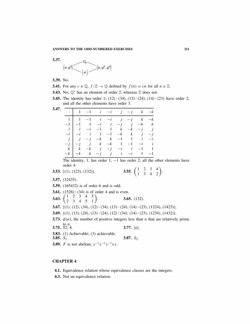
ANSWERS TO THE ODD-NUMBERED EXERCISES 311
3.37. C6
e
e, g2, g4e, g3
3.39. No.
3.41. For any c ∈ Q, f : Z → Q defined by f (n) = cn for all n ∈ Z.
3.43. No; Q∗ has an element of order 2, whereas Z does not.
3.45. The identity has order 1; (12) Ž (34), (13) Ž (24), (14) Ž (23) have order 2,and all the other elements have order 3.
3.47. · 1 −1 i −i j −j k −k
1 1 −1 i −i j −j k −k
−1 −1 1 −i i −j j −k k
i i −i −1 1 k −k −j j
−i −i i 1 −1 −k k j −j
j j −j −k k −1 1 i −i
−j −j j k −k 1 −1 −i i
k k −k j −j −i i −1 1−k −k k −j j i −i 1 −1
The identity, 1, has order 1; −1 has order 2; all the other elements haveorder 4.
3.53. {(1), (123), (132)}. 3.55.(
1 2 3 41 3 4 2
).
3.57. (12435).
3.59. (165432) is of order 6 and is odd.
3.61. (1526) Ž (34) is of order 4 and is even.
3.63.(
1 2 3 4 52 3 4 5 1
). 3.65. (132).
3.67. {(1), (12), (34), (12) Ž (34), (13) Ž (24), (14) Ž (23), (1324), (1423)}.3.69. {(1), (13), (24), (13) Ž (24), (12) Ž (34), (14) Ž (23), (1234), (1432)}.3.73. φ(n), the number of positive integers less than n that are relatively prime
to n.3.75. 52; 8. 3.77. {e}.3.83. (1) Achievable; (3) achievable.3.85. S3. 3.87. S2.
3.89. F is not abelian; y−1x−1y−1xx.
CHAPTER 4
4.1. Equivalence relation whose equivalence classes are the integers.
4.3. Not an equivalence relation.

312 ANSWERS TO THE ODD-NUMBERED EXERCISES
4.5. Left Cosets Right Cosets
H = {(1), (12), (34), (12) Ž (34)} H = {(1), (12), (34), (12) Ž (34)}(13)H = {(13), (123), (134), (1234)} H(13) = {(13), (132), (143), (1432)}(14)H = {(14), (124), (143), (1243)} H(14) = {(14), (142), (134), (1342)}(23)H = {(23), (132), (234), (1342)} H(23) = {(23), (123), (243), (1243)}(24)H = {(24), (142), (243), (1432)} H(24) = {(24), (124), (234), (1234)}
(1324)H = {(1324), (14) Ž (23), H(1324) = {(1324), (13) Ž (24),(13) Ž (24), (1423)} (14) Ž (23), (1423)}
4.7. Not a morphism.4.9. A morphism; Kerf = 4Z, and Imf = {(0, 0), (1, 1), (0, 2), (1, 3)}.
4.11. Not a morphism. 4.19. No.4.21. f : C3 → C4 defined by f (gr) = e.4.23. fk: C6 → C6 defined by fk(g
r) = gkr for k = 0, 1, 2, 3, 4, 5.4.25. Not isomorphic; C60 contains elements of order 4, whereas C10 × C6
does not.4.27. Not isomorphic; Cn × C2 is commutative, whereas Dn is not.4.29. Not isomorphic; (1 + i)/
√2 has order 8, whereas Z4 × Z2 contains no
element of order 8.4.33. C10 and D5. 4.39. (R+, ·).4.49. G2
∼= S3.4.59. 5 is a generator of Z∗
6, and 3 is a generator of Z∗17.
CHAPTER 5
5.1. C2 and C2. 5.3. C2 and C2 × C2.5.5. C3 and D3. 5.7. C9 and C9.5.9. D4. 5.11. S4.
5.13. S4. 5.15. S4.5.17. A5. 5.19. A5.5.21. A5. 5.25. S4.
5.27.
−1 0 0
0 −1 00 0 1
and
0 0 1
1 0 00 1 0
.
5.29. D6. 5.31. C2.
5.33. D4 generated by
−1 0 0
0 1 00 0 −1
and
0 −1 0
1 0 00 0 1
.
CHAPTER 6
6.1. 3. 6.3. 38.6.5. 78. 6.7. 35.
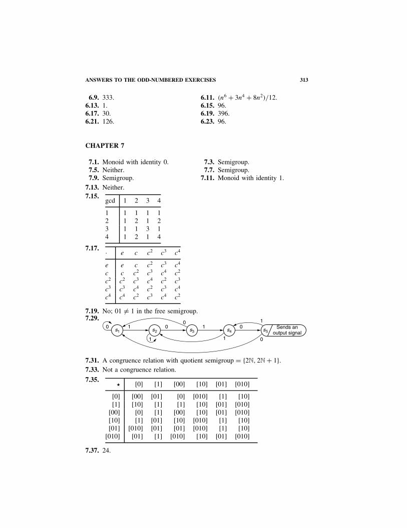
ANSWERS TO THE ODD-NUMBERED EXERCISES 313
6.9. 333. 6.11. (n6 + 3n4 + 8n2)/12.6.13. 1. 6.15. 96.6.17. 30. 6.19. 396.6.21. 126. 6.23. 96.
CHAPTER 7
7.1. Monoid with identity 0. 7.3. Semigroup.7.5. Neither. 7.7. Semigroup.7.9. Semigroup. 7.11. Monoid with identity 1.
7.13. Neither.7.15.
gcd 1 2 3 4
1 1 1 1 12 1 2 1 23 1 1 3 14 1 2 1 4
7.17. · e c c2 c3 c4
e e c c2 c3 c4
c c c2 c3 c4 c2
c2 c2 c3 c4 c2 c3
c3 c3 c4 c2 c3 c4
c4 c4 c2 c3 c4 c2
7.19. No; 01 �= 1 in the free semigroup.7.29.
s1 s2 s3 s4 s5Sends an
output signal1 0
00 1
1
1 0
0
1
7.31. A congruence relation with quotient semigroup = {2N, 2N + 1}.7.33. Not a congruence relation.
7.35.� [0] [1] [00] [10] [01] [010]
[0] [00] [01] [0] [010] [1] [10][1] [10] [1] [1] [10] [01] [010]
[00] [0] [1] [00] [10] [01] [010][10] [1] [01] [10] [010] [1] [10][01] [010] [01] [01] [010] [1] [10]
[010] [01] [1] [010] [10] [01] [010]
7.37. 24.

314 ANSWERS TO THE ODD-NUMBERED EXERCISES
7.39.� [�] [α] [β] [γ ] [αβ] [αγ ]
[�] [�] [α] [β] [γ ] [αβ] [αγ ][α] [α] [�] [αβ] [αγ ] [β] [γ ][β] [β] [β] [β] [γ ] [β] [γ ][γ ] [γ ] [γ ] [γ ] [β] [γ ] [β][αβ] [αβ] [αβ] [αβ] [αγ ] [αβ] [αγ ][αγ ] [αγ ] [αγ ] [αγ ] [αβ] [αγ ] [αβ]
7.41.s1
0
1s0
0, 1
7.43.
s010
s10
0
s00
0
1
0
1 1
s11
1
{[0], [1]}. {[0], [1], [10]}.7.45. The monoid contains 27 elements.
Dormant1
WCF
Dormant2
R
Dormant3
R
R
CF
CF
WBuds
RWC
WDead
RWCF
F
CHAPTER 8
8.1. + 0 1 2 3
0 0 1 2 31 1 2 3 02 2 3 0 13 3 0 1 2
· 0 1 2 3
0 0 0 0 01 0 1 2 32 0 2 0 23 0 3 2 1
8.3. A ring.8.5. Not a ring; not closed under multiplication.8.7. Not a ring; not closed under addition.8.9. A ring.
8.11. Not a ring; distributive laws do not hold.8.17. A subring.8.19. Not a subring; not closed under addition.8.21. Neither. 8.23. Both.8.25. Integral domain. 8.29. [2], [4], [5], [6], [8].

ANSWERS TO THE ODD-NUMBERED EXERCISES 315
8.31. Any nonempty proper subset of X.8.33. Nonzero matrices with zero determinant.8.37. f (x) = [x]6.8.39. f (x, y) = (x, y), (y, x), (x, x) or (y, y).8.47. (b) −1 and 0.8.55. The identity is Dn(x) = (1/2π) + (1/π)(cos x + cos 2x + · · · + cos nx).
The ring is not an integral domain.
CHAPTER 9
9.1. 32x2 + 5
4x − 158 and 45
8 x + 78 .
9.3. x4 + x3 + x2 + x and 1.9.5. 3 − i and 4 + 2i, or 4 − i and 1 − 2i, or 4 − 2i and −3 + i.9.7. gcd(a, b) = 3, s = −5, t = 4.9.9. gcd(a, b) = 1, s = −(2x + 1)/3, t = (2x + 2)/3.
9.11. gcd(a, b) = 2x + 1, s = 1, t = 2x + 1.9.13. gcd(a, b) = 1, s = 1, t = −1 + 2i.9.15. x = −6, y = 5. 9.17. x = −14, y = 5.9.19. [23]. 9.21. [17].9.23. No solutions. 9.25. (x − 1)(x4 + x3 + x2 + x + 1).9.27. (x2 + 2)(x2 + 3). 9.29. x4 − 9x + 3.
9.31. x3 − 4x + 1.9.33. (x − √
2)(x + √2)(x − i
√2)(x + i
√2)(x − 1 − i)(x − 1 + i)
(x + 1 − i)(x + 1 + i).9.35. (x2 − 2)(x2 + 2)(x2 − 2x + 2)(x2 + 2x + 2).9.37. x5 + x3 + 1, x5 + x2 + 1, x5 + x4 + x3 + x2 + 1, x5 + x4 + x3 + x + 1,
x5 + x4 + x2 + x + 1, x5 + x3 + x2 + x + 1.9.39. x3 + 2.9.41. Kerψ = {q(x) · (x2 − 2x + 4)|q(x) ∈ Q[x]} and Im ψ = Q(
√3i) =
{a + b√
3i|a, b ∈ Q}.9.43. Irreducible by Eisenstein’s Criterion.9.45. Irreducible, since it has no linear factors.9.47. Reducible; any polynomial of degree >2 in R[x] is reducible.9.49. No. 9.55. No.9.61. x ≡ 40 mod 42. 9.63. x ≡ 22 mod 30.9.67. 65.
CHAPTER 10
10.1. ((0, 0)), ((0, 1)), ((1, 0)), Z2 × Z2.10.3. (0) and Q.
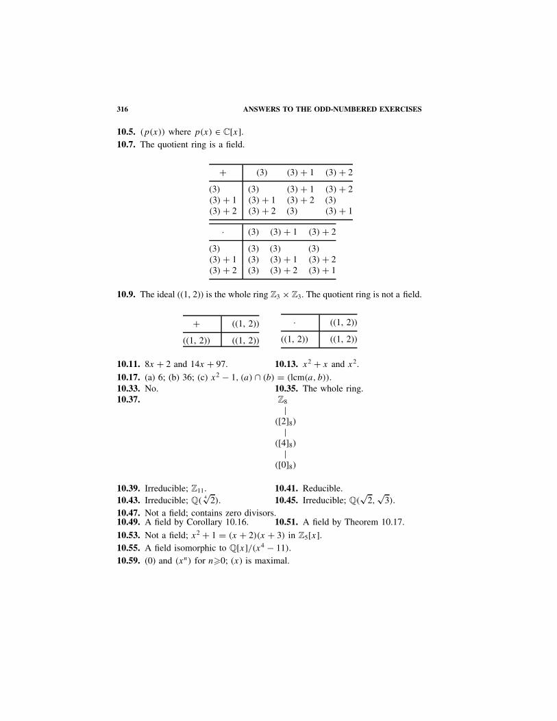
316 ANSWERS TO THE ODD-NUMBERED EXERCISES
10.5. (p(x)) where p(x) ∈ C[x].10.7. The quotient ring is a field.
+ (3) (3) + 1 (3) + 2
(3) (3) (3) + 1 (3) + 2(3) + 1 (3) + 1 (3) + 2 (3)(3) + 2 (3) + 2 (3) (3) + 1
· (3) (3) + 1 (3) + 2
(3) (3) (3) (3)(3) + 1 (3) (3) + 1 (3) + 2(3) + 2 (3) (3) + 2 (3) + 1
10.9. The ideal ((1, 2)) is the whole ring Z3 × Z3. The quotient ring is not a field.
+ ((1, 2))
((1, 2)) ((1, 2))
· ((1, 2))
((1, 2)) ((1, 2))
10.11. 8x + 2 and 14x + 97. 10.13. x2 + x and x2.
10.17. (a) 6; (b) 36; (c) x2 − 1, (a) ∩ (b) = (lcm(a, b)).10.33. No. 10.35. The whole ring.10.37. Z8
|([2]8)
|([4]8)
|([0]8)
10.39. Irreducible; Z11. 10.41. Reducible.10.43. Irreducible; Q(
4√
2). 10.45. Irreducible; Q(√
2,√
3).10.47. Not a field; contains zero divisors.10.49. A field by Corollary 10.16. 10.51. A field by Theorem 10.17.
10.53. Not a field; x2 + 1 = (x + 2)(x + 3) in Z5[x].10.55. A field isomorphic to Q[x]/(x4 − 11).10.59. (0) and (xn) for n�0; (x) is maximal.

ANSWERS TO THE ODD-NUMBERED EXERCISES 317
CHAPTER 11
11.1. GF(5) = Z5 = {0, 1, 2, 3, 4}.
+ 0 1 2 3 4
0 0 1 2 3 41 1 2 3 4 02 2 3 4 0 13 3 4 0 1 24 4 0 1 2 3
· 0 1 2 3 4
0 0 0 0 0 01 0 1 2 3 42 0 2 4 1 33 0 3 1 4 24 0 4 3 2 1
11.3. GF(9) = Z3[x]/(x2 + 1) = {aα + b|a, b ∈ Z3, α2 + 1 = 0}.
+ 0 1 2 α α + 1 α + 2 2α 2α + 1 2α + 2
0 0 1 2 α α + 1 α + 2 2α 2α + 1 2α + 21 1 2 0 α + 1 α + 2 α 2α + 1 2α + 2 2α
2 2 0 1 α + 2 α α + 1 2α + 2 2α 2α + 1α α α +1 α + 2 2α 2α + 1 2α + 2 0 1 2α + 1 α + 1 α +2 α 2α + 1 2α + 2 2α 1 2 0α + 2 α + 2 α α + 1 2α + 2 2α 2α + 1 2 0 1
2α 2α 2α +1 2α + 2 0 1 2 α α + 1 α + 22α + 1 2α + 1 2α +2 2α 1 2 0 α + 1 α + 2 α
2α + 2 2α + 2 2α 2α + 1 2 0 1 α + 2 α α + 1
· 0 1 2 α α + 1 α + 2 2α 2α + 1 2α + 2
0 0 0 0 0 0 0 0 0 01 0 1 2 α α + 1 α + 2 2α 2α + 1 2α + 22 0 2 1 2α 2α + 2 2α + 1 α α + 2 α + 1
α 0 α 2α 2 α + 2 2α + 2 1 α + 1 2α + 1α + 1 0 α + 1 2α +2 α + 2 2α 1 2α + 1 2 α
α + 2 0 α + 2 2α +1 2α + 2 1 α α + 1 2α 22α 0 2α α 1 2α + 1 α + 1 2 2α + 2 α + 22α + 1 0 2α + 1 α +2 α + 1 2 2α 2α + 2 α 12α + 2 0 2α + 2 α +1 2α + 1 α 2 α + 2 1 2α
11.5. x3 + x + 4. 11.7. Impossible.11.9. x2 + 2. 11.11. x4 − 16x2 + 16.
11.13. 8x6 − 9. 11.17. 3.

318 ANSWERS TO THE ODD-NUMBERED EXERCISES
11.19. 2. 11.21. 2.11.23. ∞. 11.25. ∞.11.27. (1 − 3
√2 + 3
√4)/3. 11.29. −(1 + 6ω)/31.
11.31. α4 + α. 11.33. 2; not a field.11.35. 7; a field 11.37. 0; a field.11.39. 0; not a field.11.43. m = 2, 4, pr or 2pr , where p is an odd prime; see Weiss [12, Th. 4–6–10].
11.47. α = √2 + √−3.
11.49. All elements of GF(32) except 0 and 1 are primitive.11.51. x3 + x + 1. 11.57. No solutions.11.59. x = 1 or α + 1. 11.63. 5.11.65. The output has cycle length 7 and repeats the sequence 1101001, starting
at the right.
CHAPTER 12
12.1.a b c d e f g
b c d e f g a
c d e f g a b
d e f g a b c
e f g a b c d
f g a b c d e
g a b c d e f
12.3. Use GF(8) = {0, 1, α, 1 + α, α2, 1 + α2, α + α2, 1 + α + α2} whereα3 = α + 1.
12.7. No.12.9.
Week
1 2 3 4
↓ ↓ ↓ ↓→ A B C D
Shelf → B C D A
height → C D A B
→ D A B C
A, B, C, and D are the four brands of cereal.

ANSWERS TO THE ODD-NUMBERED EXERCISES 319
12.11.Week
1 2 3 4 5↓ ↓ ↓ ↓ ↓
M → A B C D 0T → B C D 0 A
W → C D 0 A B
T → D 0 A B C
F → 0 A B C D
A, B, C, and D are the four different types of music, and 0 refers tono music.
12.15. y = αx. 12.17. y = (α + 2)x + 2α.12.21. 1.12.23.
1 6 11 1612 15 2 514 9 8 37 4 13 10
1 6 11 1615 12 5 28 3 14 9
10 13 4 7
12.25.1 10 19 28 37 46 55 64
35 44 49 58 7 16 21 3029 22 15 8 57 50 43 3663 56 45 38 27 20 9 252 59 34 41 24 31 6 1318 25 4 11 54 61 40 4748 39 62 53 12 3 26 1714 5 32 23 42 33 60 51
CHAPTER 13
13.1. Constructible. 13.3. Constructible.13.5. Not constructible. 13.7. No.
13.11. Yes. 13.13. No.
13.15. Yes;π
21= 1
4
(π
3− π
7
). 13.23. Yes.
13.25. No. 13.27. No.13.29. Yes. 13.31. No.13.33. Yes.
CHAPTER 14
14.1. 010, 001, 111.

320 ANSWERS TO THE ODD-NUMBERED EXERCISES
14.3. The checking is done modulo 9, using the fact that any integer is congruentto the sum of its digits modulo 9.
14.5. (1 2 3 4 5 6 7 8 9 10) modulo 11. It will detect one error but notcorrect any.
14.7. 000000, 110001, 111010, 001011, 101100, 011101, 010110, 100111.14.9. 101, 001, 100.
14.11. Minimum distance = 3. It detects two errors and corrects one error.
H =
1 0 0 0 0 0 0 1 00 1 0 0 0 0 1 0 10 0 1 0 0 1 0 1 10 0 0 1 0 0 1 0 00 0 0 0 1 1 0 0 1
.
14.13. GT = (1 1 1 1
),H =
1 0 0 1
0 1 0 10 0 1 1
.
14.15. GT =
1 0 1 0 0 1 0 0 00 1 0 1 0 0 1 0 00 0 1 0 1 0 0 1 01 0 1 1 0 0 0 0 1
,
H =
1 0 0 0 0 1 0 0 10 1 0 0 0 0 1 0 00 0 1 0 0 1 0 1 10 0 0 1 0 0 1 0 10 0 0 0 1 0 0 1 0
.
14.17. 110, 010, 101, 001, 011.14.19.
Syndrome Coset Leader
00 00001 01010 10011 001

ANSWERS TO THE ODD-NUMBERED EXERCISES 321
14.21.Coset Coset Coset
Syndrome Leader Syndrome Leader Syndrome Leader
00000 000000000 01011 000010100 10110 00000000100001 000010000 01100 011000000 10111 00001000100010 000100000 01101 010000010 11000 11000000000011 000110000 01110 001000100 11001 00000011100100 001000000 01111 000000110 11010 10000010000101 000000010 10000 100000000 11011 00000111000110 001100000 10001 000001010 11100 00000010100111 000100010 10010 100100000 11101 00001010101000 010000000 10011 000000011 11110 00000110001001 010010000 10100 000001000 11111 000011100
01010 000000100 10101 000011000
14.23. (a) 56; (b) 7; (c) 27 = 128, (d) 8/9; (e) it will detect single, double, triple,and any odd number of errors; (f) 1.
14.25. No.14.29. x8 + x4 + x2 + x + 1 and x10 + x9 + x8 + x6 + x5 + x2 + 1.14.31. x5 + x4 + x3 + x2 + 1.

INDEX
Abel, N. H., 1, 47, 48Abelian group, 48
finite, 92Absorption laws, 15Abstract algebra, 2Action of a group, 96Adder, full, 35
half, 34modulo 2, 28serial, 152
Addition modulo m, 84Adjoining an element, 220Affine plane, 242Algebra, abstract, 2
boolean, 7, 14, 25classical, 1modern, 2
Algebraic numbers, 221, 233Algebraic structure, 4Algebra of sets, 7Alternating group, 70, 81, 85, 88AND gate, 36Angle trisection, 251, 257Antisymmetry, 23Archimedean solids, 121Archimedes, 258Associativity, 3, 14, 48, 137, 155Atom, 26Automorphism, 75, 151
Frobenius, 235Axiomatic method, 295Axioms, 295Axis of symmetry, 51
BCH code, 284Benzene, 126
Biconditional, 18Bijective, 50, 63Binary code, 266Binary operation, 2Binary symmetric channel, 266Binomial theorem, 178
coefficients, 129Boole, G., 7Boolean algebra, 7, 14, 25
isomorphism, 39morphism, 39representation theorem, 39
Boolean expression, 26Boolean ring, 158, 176Bose, R. C., 242, 284Bridge circuit, 43Burnside, W., 125Burnside’s theorem (lemma), 125
Cancellation, 53Cantor’s theorem, 41Carrol, L., 41Casting out nines, 288Cauchy sequences, 6Cayley, A., 47, 71Cayley’s theorem, 71CD, 264Center of a group, 74Characteristic of a ring, 226Check digit, 266Chinese remainder theorem, 198Circle group, 88, 98Circle squaring, 251, 259Circuit, see Switching circuitsClassical algebra, 1Closed switch, 19
Modern Algebra with Applications, Second Edition, by William J. Gilbert and W. Keith NicholsonISBN 0-471-41451-4 Copyright 2004 John Wiley & Sons, Inc.
323

324 INDEX
Closure of an operation, 3, 48Code, 264
BCH, 284binary, 266cyclic, 292error-correcting, 265error-detecting, 264linear, 276(n, k)-, 266parity check, 267, 274polynomial, 270repeating, 268
Code rate, 267Code word, 266Coefficient, 166Colorings, 128Common divisor, 184, 299
multiple, 184, 303Commutativity, 3, 14, 48, 148, 167Commutator, 101Complement, 8, 14Complex numbers, 4, 223Complex roots, 191Composition of relations, 150
of functions, 49of relations, 150
Conclusion, 293Concatenation, 140Conditional, 17Cone, n-agonal, 116Congruence, 77, 79, 145
linear, 197Congruence class, 77, 145Conjugate, 191Conjunctive normal form, 45Constant polynomial, 167Constructible number, 252Constructible point, 252Construction of polygons, 259Contradiction, 17
proof by, 294Converse, 295Convolution fraction, 175Convolution of functions, 173
of sequences, 168Coset, 79, 82Coset leader, 280Countable, 221Counterexample, 295Cross-ratio, 101Crystalline lattice, 120Crystallographic group, 120Cube, duplication of, 251, 256Cube, rotation group of, 114
Cycle, 64disjoint, 66
Cyclic code, 291Cyclic group, 56Cyclic monoid, 139, 150Cyclic subgroup, 57Cyclotomic polynomial, 195Cylinder, n-agonal, 116
Da Vinci, L., 109Decode, 280Dedekind cuts, 6Degree, of an extension, 219
of a polynomial, 166Delta function, 172De Morgan’s laws, 15Derivative, 292Detecting errors, 280Determinant, 110, 112, 287Diagram, state, 143
tree, 148Venn, 8, 32
Difference, 9symmetric, 9
Dihedral group, 58, 90Dirac delta function, 172Direct product, 2, 91, 164Direct sum, 91Disjoint cycles, 66Disjunctive normal form, 30Distributions, 175Distributivity, 4, 14, 156Division, 184, 299Division algorithm, 180, 181, 298Divisor of zero, 159Dodecahedron, 112
rotation group, 114Domain, 172
left Ore, 172Domain, integral, 159Duality in boolean algebras, 15Duality of regular solids, 112Duplication of the cube, 251, 256Durer, A., 246DVD, 264
Eigenvalue, 108, 109, 111Eigenvector, 108, 110Eisenstein’s criterion, 194Element of a set, 7Empty set, 7Encode, 266, 280Encoding matrix, 276Endomorphism ring, 178

INDEX 325
Equivalence class, 77Equivalence, logical, 295Equivalence relation, 5, 77Equivalent circuits, 20Error-correcting code, 264Error-detecting code, 264Error polynomial, 275Euclidean algorithm, 185, 300Euclidean group, 104Euclidean ring, 181Euclid’s lemma, 302Euclid’s theorem, 298Euler, L., 103, 236, 242, 260Euler φ-function, 103Even permutation, 68Exclusive OR, 10, 29Extension field, 218
degree of, 219finite, 219
Factor, 184, see also QuotientFactor theorem, 182Faithful action of a group, 96Faithful representation, 109Feedback shift register, 231, 272Fermat, P., 103, 260Fermat primes, 260Fermat’s last theorem, 305Field, 4, 160
finite, 6, 45, 225Galois, 6, 227primitive element in, 229skew, 172
Field extension, 218Field of, convolution fractions, 175
fractions, 170quotients, 170rational functions, 172, 221
Fifteen puzzle, 74Finite, abelian group, 92
extension, 219field, 6, 45, 225geometry, 242group, 56groups in three dimensions, 116groups in two dimensions, 109
Finite-state machine, 142First isomorphism theorem, 87, 210Fixed points, 125Flip-flop, 46Formal power series, 169Fractional differentiation and integration, 175Fractions, field of, 170
left, 172
Free, group, 75monoid, 140semigroup, 140
Full adder, 35Frobenius automorphism, 235Function, bijective, 50, 63
composition of, 49delta, 172generalized, 175Heaviside, 175impulse, 172injective, 49inverse, 49one-to-one, 49onto, 50surjective, 49transition, 142
Fundamental theorem of, algebra, 6, 190arithmetic, 187
Galois, E., 6, 47, 225Galois field, 6, 227Galois theory, 47,Gate, 36Gauss, C. F., 6, 190, 260Gaussian integers, 72, 183Gauss’ lemma, 193Generalized function, 175General linear group, 107Generator, group, 56
idempotent, 292matrix, 276of a monoid, 139polynomial, 270
Geometry, 242Goldbach conjecture, 304Graeco-Latin square, see Orthogonal latin
squaresGreatest common divisor, 21, 184, 299Greatest lower bound, 25Group, 48
abelian, 48alternating, 70, 82, 86, 88automorphism, 75center, 74circle, 88, 98commutative, 48crystallographic, 120cyclic, 56dihedral, 58, 90euclidean, 104factor, 83finite, 56free, 75general linear, 107

326 INDEX
Group (continued)generator, 56icosahedral, 115infinite, 56isomorphism, 60Klein, 52, 90matrix, 107metabelian, 102morphism, 60noncommutative, 59octahedral, 114of a polynomial, 80of a rectangle, 53, 55of a square, 89of low order, 94of prime order, 80order, 56orthogonal, 105permutation, 50quaternion, 73, 95, 107quotient, 83simple, 86special orthogonal, 98, 108special unitary, 108sporadic, 86symmetric, 50, 63symmetries, 51tetrahedral, 113translation, 49, 104trivial, 49unitary, 108
Group acting on a set, 96Group isomorphism, 60Group morphism, 60
Half adder, 34Hamming distance, 268Heaviside, O., 172, 175Homomorphism, see MorphismHypothesis, 293
Icosahedral group, 115Icosahedron, 112
rotation group, 114Ideal, 204
left, 217maximal, 216prime, 216principal, 204
Ideal crystalline lattice, 120Idempotent element, 179
generator, 292laws, 15
Identity, 4, 48, 137function, 49
If and only if, 18, 295Image, 87Implication, 17, 293Improper rotation, 52, 58, 108Impulse functions, 172Inclusion, 7Index of a subgroup, 80Induction, 296
extended, 297strong, 297
Infinite group, 56Information rate, 267Injective, 49, 86Input values, 142Integers, 5, 156, 296
gaussian, 72, 183Integers modulo m, 78Integral domain, 159Interlacing shuffle, 74International standard book number, 289Intersection of sets, 8Inverse, 3, 48, 188
function, 49Inversion theorem, 50Invertible element, 3, 48, 188Irrational roots, 192Irreducible, 189
polynomial, 190Isometry, 51, 112Isomorphism, 5
boolean algebra, 39group, 60monoid, 141ring, 162
Isomorphism theorems for groups, 87, 101,102
Isomorphism theorems for rings, 210, 215
Join, 14Juxtaposition, 140
Kernel, 86Klein, F., 52Klein 4-group, 52, 90Kronecker, L., 5
Lagrange, J., 79Lagrange’s theorem, 80Latin square, 236
orthogonal, 239Lattice, 25
crystalline, 120

INDEX 327
Least common multiple, 21, 184, 303Least upper bound, 25Left coset, 82Left ideal, 217Linear code, 276
cyclic, 291Linear congruences, 197,Linear transformation, 5, 104Lines in a geometry, 242Length of a vector, 105Local ring, 216Logically equivalent, 17, 295Logic of propositions, 16
Machine, 142monoid of, 145parity checker, 143semigroup of, 142
Magic square, 247Mathematical theory, 295Matrix
eigenvalue of, 108eigenvector of, 108encoding, 276generator, 276nonsingular, 4orthogonal, 105parity check, 278unitary, 108
Matrix group, 107Matrix representation, 109
of codes, 276Matrix ring, 166Maximal ideal, 216Meet, 14Metabelian group, 102Metric, 291Mikusinski, J., 173Modern algebra, 2Modular representation, 200Modulo m, 78Modulo 2 adder, 28Monic polynomial, 234Monoid, 137
automorphism, 151cyclic, 139, 150free, 140generator, 139morphism, 141morphism theorem, 150quotient, 145representation theorem, 150transformations, 138
Monoid isomorphism, 141
Monoid morphism, 141Monoid of a machine, 145Monoid of transformations, 138Morphism, 5
boolean algebra, 39group, 60monoid, 141ring, 172
Morphism theorem for, groups, 87, 101, 102monoids, 150rings, 210
Mutually orthogonal squares, 239
NAND gate, 28, 36Necklace problems, 126Network, see Switching circuitsNilpotent element, 216Nonsingular matrix, 4NOR gate, 28, 36Normal form, conjunctive, 45
disjunctive, 30Normal subgroup, 82NOT gate, 36
Octahedral group, 114Octahedron, 112
rotation group, 114Odd permutation, 68One-to-one, 49One-to-one correspondence, 50Onto, 50Open switch, 19Operation, 2Operational calculus, 172Operator, 175Orbit, 65, 78, 97Order of a group, 56Order of an element, 56OR gate, 36Orthogonal group, 105Orthogonal latin squares, 239Orthogonal matrix, 105Output, 142
Parallel circuit, 19Parallelism, 242Parity check, 278
code, 267, 274machine, 143matrix, 278
Parity of a permutation, 69Partial order, 24Partition, 77Pattern recognition, 147

328 INDEX
Permutation, 50, 63even, 68odd, 68parity, 69
Permutation group, 50, 63Phi function, 103Plane, affine, 242
projective, 245Points of a geometry, 242Pole of a rotation, 116Polya, G., 125, 134Polya-Burnside enumeration, 124Polygons, construction, 259Polyhedron, dual, 112Polynomial, 166
coefficients, 166constant, 167cyclotomic, 195degree, 166equality, 166group of symmetries, 74irreducible, 189, 190monic, 234primitive, 231, 275reducible, 190zero, 166
Polynomial code, 270Polynomial equations, 1, 47Polynomial representation of codes, 270Polynomial ring, 167Poset, 24Positive integers, 3Power series, 169Power set, 8Prime, 189, 294, 297
factorization theorem, 21, 302Fermat, 260ideal, 216
Prime order group, 80Primitive element, 229Primitive polynomial, 231, 275Principal ideal, 204Principal ideal ring, 205Product group, 91Product ring, 164Projective plane, 245Projective space, 102Proof, 293
by contradiction, 294by reduction to cases, 293direct, 293
Proper rotation, 52, 58, 108symmetry, 52
Propositional calculus, 18
Quaternion, group, 73, 95, 107ring, 172, 177
Quotient, 181, 299field of, 170group, 83monoid, 145ring, 206set, 72structure, 5
Radical of a ring, 216Rational functions, 172, 221Rational number, 6, 48, 78, 170Rational roots theorem, 192Real numbers, 6, 48, 156Real numbers modulo one, 88Real projective space, 102Rectangle, symmetries of, 53, 55Reducible, 190Redundant digits, 267Reflexivity, 23, 77Register, shift, 231, 272Regular n-gon, rotations, 58Regular polygons, construction, 259Regular solid, 112Relation, 76
composition of, 150congruence, 77, 145equivalence, 77partial order, 24
Relatively prime, 301Remainder, 181, 299Remainder theorem, 182Repeating code, 268Representation, faithful, 109
matrix, 109modular, 200residue, 200
Representation theorem for, booleanalgebras, 39, 40groups, 71monoids, 150
Representative of a coset, 79Residue representation, 200Right coset, 79Ring, 155
boolean, 158, 176characteristic, 226commutative, 156endomorphism, 178euclidean, 181factor, 206field, 160ideal of, 204

INDEX 329
integral domain, 159local, 216matrix, 166morphism, 172morphism theorem, 210nontrivial, 159polynomial, 166principal ideal, 205product, 164quotient, 206radical of, 216simple, 217subring of, 161trivial, 159
Ring isomorphism, 162Ring morphism, 162, 210Ring of, formal power series, 169
matrices, 166polynomials, 166quaternions, 172, 177sequences, 168
Roots, 183complex, 190, 191irrational, 191rational, 192
Rotations, 52, 58, 108Rotations of, a cube, 114
a dodecahedron, 114an icosahedron, 114an n-gon, 58an octahedron, 114a tetrahedron, 113
Ruler and compass, 251
Second isomorphism theorem, 102, 215Semigroup, 137
free, 140Semigroup of a machine, 145Sequences, ring of, 168Serial adder, 152Series, power, 169Series circuit, 19Series-parallel circuit, 20Set, 7Sets, algebra of, 7Shannon, C. E., 267Shift register, 231, 272Shuffle, interlacing, 74Simple, group, 86
ring, 217Simplification of circuits, 26Skew field, 172Smallest subfield, 220Solids, Archimedean, 121
Solids, regular, 112Space, projective, 102Special orthogonal group, 98, 108Special unitary group, 108Sphere, 116Sporadic groups, 86Square, latin, 236
magic, 247orthogonal latin, 239
Square-free integer, 22, 302Squaring the circle, 251, 259Stabilizer, 97Standard basis, 104Standard matrix, 105, 164State, 142
diagram, 143Step function, 175Stone’s representation theorem, 40Straight-edge and compass constructions, 251Structure, algebraic, 4Structure, quotient, 5Subfield, 218
smallest, 220Subgroup, 54
commutator, 101cyclic, 57index of, 80normal, 92
Submonoid, 150Subring, 161Subset, 7Substructure, 4Sum, direct, 91Surjective, 49Switch, 19Switching circuits, 20
bridge, 43number of, 130n-variable, 28series-parallel, 28
Switching function, 27Sylow theorems, 85Symmetric condition, 23, 77Symmetric difference, 9, 28Symmetric group, 50, 63Symmetries of a
figure, 3, 51polynomial, 74rectangle, 53, 55set, 50square, 89
Symmetry, proper, 52Syndrome, 280
330 INDEX
Table, 3truth, 16
Tarry, G., 242Tautology, 17Tetrahedral group, 113Tetrahedron, 112
rotation group, 113Third isomorphism theorem, 102, 215Titchmarsh’s theorem, 174Transcendental, 221Transformation monoid, 138Transient conditions in circuits, 49Transistor gates, 36Transition function, 142Transitivity, 23, 77Translation, 49, 104Transpose of a matrix, 104Transposition, 68Tree diagram, 148Trisection of an angle, 251, 257Trivial group, 49Trivial ring, 159Truth table, 16
Unary operation, 2, 8, 14Underlying set, 4Union of sets, 8Unique factorization theorem, 189Unitary group, 108Unit element, 188. See also Identity;
Invertible elementUnity, see IdentityUniversal bounds, 25
Vandermonde determinant, 287Vector space, 5Venn diagram, 8, 32
Well ordering axiom, 296Wilson’s theorem, 202Words, 140
Zero, 14, 155Zero divisor, 159Zero polynomial, 166

PURE AND APPLIED MATHEMATICSA Wiley-Interscience Series of Texts, Monographs, and Tracts
Founded by RICHARD COURANTEditors: MYRON B. ALLEN III, DAVID A. COX, PETER LAXEditors Emeriti: PETER HILTON, HARRY HOCHSTADT, JOHN TOLAND
ADAMEK, HERRLICH, and STRECKER—Abstract and Concrete CategoriesADAMOWICZ and ZBIERSKI—Logic of MathematicsAINSWORTH and ODEN—A Posteriori Error Estimation in Finite Element AnalysisAKIVIS and GOLDBERG—Conformal Differential Geometry and Its GeneralizationsALLEN and ISAACSON—Numerical Analysis for Applied Science∗ARTIN—Geometric AlgebraAUBIN—Applied Functional Analysis, Second EditionAZIZOV and IOKHVIDOV—Linear Operators in Spaces with an Indefinite MetricBERG—The Fourier-Analytic Proof of Quadratic ReciprocityBERMAN, NEUMANN, and STERN—Nonnegative Matrices in Dynamic SystemsBERKOVITZ—Convexity and Optimization in Rn
BOYARINTSEV—Methods of Solving Singular Systems of Ordinary DifferentialEquations
BURK—Lebesgue Measure and Integration: An Introduction∗CARTER—Finite Groups of Lie TypeCASTILLO, COBO, JUBETE, and PRUNEDA—Orthogonal Sets and Polar Methods in
Linear Algebra: Applications to Matrix Calculations, Systems of Equations,Inequalities, and Linear Programming
CASTILLO, CONEJO, PEDREGAL, GARCIA, and ALGUACIL—Building and SolvingMathematical Programming Models in Engineering and Science
CHATELIN—Eigenvalues of MatricesCLARK—Mathematical Bioeconomics: The Optimal Management of Renewable
Resources, Second Edition†COX—Primes of the Form x2 + ny2: Fermat, Class Field Theory, and Complex
Multiplication∗CURTIS and REINER—Representation Theory of Finite Groups and Associative
Algebras∗CURTIS and REINER—Methods of Representation Theory: With Applications to Finite
Groups and Orders, Volume ICURTIS and REINER—Methods of Representation Theory: With Applications to Finite
Groups and Orders, Volume IIDINCULEANU—Vector Integration and Stochastic Integration in Banach Spaces∗DUNFORD and SCHWARTZ—Linear Operators
Part 1—General TheoryPart 2—Spectral Theory, Self Adjoint Operators in
Hilbert SpacePart 3—Spectral Operators
∗ Now available in a lower priced paperback edition in the Wiley Classics Library.† Now available in paperback.
Modern Algebra with Applications, Second Edition, by William J. Gilbert and W. Keith NicholsonISBN 0-471-41451-4 Copyright 2004 John Wiley & Sons, Inc.

FARINA and RINALDI—Positive Linear Systems: Theory and ApplicationsFOLLAND—Real Analysis: Modern Techniques and Their ApplicationsFROLICHER and KRIEGL—Linear Spaces and Differentiation TheoryGARDINER—Teichmuller Theory and Quadratic DifferentialsGILBERT and NICHOLSON—Modern Algebra with Applications, Second EditionGREENE and KRANTZ—Function Theory of One Complex Variable∗GRIFFITHS and HARRIS—Principles of Algebraic GeometryGRILLET—AlgebraGROVE—Groups and CharactersGUSTAFSSON, KREISS and OLIGER—Time Dependent Problems and Difference
MethodsHANNA and ROWLAND—Fourier Series, Transforms, and Boundary Value Problems,
Second Edition∗HENRICI—Applied and Computational Complex Analysis
Volume 1, Power Series—Integration—Conformal Mapping—Locationof Zeros
Volume 2, Special Functions—Integral Transforms—Asymptotics—Continued Fractions
Volume 3, Discrete Fourier Analysis, Cauchy Integrals, Constructionof Conformal Maps, Univalent Functions
∗HILTON and WU—A Course in Modern Algebra∗HOCHSTADT—Integral EquationsJOST—Two-Dimensional Geometric Variational ProceduresKHAMSI and KIRK—An Introduction to Metric Spaces and Fixed Point Theory∗KOBAYASHI and NOMIZU—Foundations of Differential Geometry, Volume I∗KOBAYASHI and NOMIZU—Foundations of Differential Geometry, Volume IIKOSHY—Fibonacci and Lucas Numbers with ApplicationsLAX—Functional AnalysisLAX—Linear AlgebraLOGAN—An Introduction to Nonlinear Partial Differential EquationsMcCONNELL and ROBSON—Noncommutative Noetherian RingsMORRISON—Functional Analysis: An Introduction to Banach Space TheoryNAYFEH—Perturbation MethodsNAYFEH and MOOK—Nonlinear OscillationsPANDEY—The Hilbert Transform of Schwartz Distributions and ApplicationsPETKOV—Geometry of Reflecting Rays and Inverse Spectral Problems∗PRENTER—Splines and Variational MethodsRAO—Measure Theory and IntegrationRASSIAS and SIMSA—Finite Sums Decompositions in Mathematical AnalysisRENELT—Elliptic Systems and Quasiconformal MappingsRIVLIN—Chebyshev Polynomials: From Approximation Theory to Algebra and Number
Theory, Second EditionROCKAFELLAR—Network Flows and Monotropic OptimizationROITMAN—Introduction to Modern Set Theory∗RUDIN—Fourier Analysis on GroupsSENDOV—The Averaged Moduli of Smoothness: Applications in Numerical Methods
and Approximations
∗ Now available in a lower priced paperback edition in the Wiley Classics Library.†Now available in paperback.

SENDOV and POPOV—The Averaged Moduli of Smoothness∗SIEGEL—Topics in Complex Function Theory
Volume 1—Elliptic Functions and Uniformization TheoryVolume 2—Automorphic Functions and Abelian IntegralsVolume 3—Abelian Functions and Modular Functions of Several Variables
SMITH and ROMANOWSKA—Post-Modern AlgebraSTAKGOLD—Green’s Functions and Boundary Value Problems, Second Edition∗STOKER—Differential Geometry∗STOKER—Nonlinear Vibrations in Mechanical and Electrical Systems∗STOKER—Water Waves: The Mathematical Theory with ApplicationsWATKINS—Fundamentals of Matrix Computations, Second EditionWESSELING—An Introduction to Multigrid Methods†WHITHAM—Linear and Nonlinear Waves†ZAUDERER—Partial Differential Equations of Applied Mathematics, Second Edition
∗ Now available in a lower priced paperback edition in the Wiley Classics Library.† Now available in paperback.


