PHILIP M. BUCHEK MODERN CONTROL TECHNIQUES IN ACTIVE FLUTTER SUPPRESSION USING A CONTROL MOMENT GYRO (NASA-CR-138494) MODERN CONTROL N74-25532 TECHNIQUES IN ACTIVE FLUTTER SUPPRESSION USING A CONTROL MOMENT GYRO (Stanford Univ.) 1--$ p HC $8.25 CSCL 01A Unclas /o0 G3/01 . 40158 This research was supported by the National Aeronautics and Space Administration MARCH under Grant NGL 05-020-498 SUDAAR 1974 and the Traineeship Program NO. 474 https://ntrs.nasa.gov/search.jsp?R=19740017419 2018-04-19T17:55:50+00:00Z
Transcript
PHILIP M. BUCHEK
MODERN CONTROL TECHNIQUES IN ACTIVEFLUTTER SUPPRESSION USING A CONTROL MOMENT GYRO
(NASA-CR-138494) MODERN CONTROL N74-25532TECHNIQUES IN ACTIVE FLUTTER SUPPRESSIONUSING A CONTROL MOMENT GYRO (StanfordUniv.) 1--$ p HC $8.25 CSCL 01A Unclas
/o0 G3/01 . 40158
This research was supported by theNational Aeronautics and Space Administration
MARCH under Grant NGL 05-020-498 SUDAAR1974 and the Traineeship Program NO. 474
Department of Aeronautics and AstronauticsStanford UniversityStanford, California
MODERN CONTROL TECHNIQUES IN ACTIVE FLUTTER SUPPRESSION
USING A CONTROL MOMENT GYRO
by
Philip M. Buchek
SUDAAR NO. 474
March 1974
This research was supported by theNational Aeronautics and Space Administration
under Grant NGL 05-020- 498and the Traineeship Program
/
ABSTRACT
PRDBCEDING PAGE BLANK NOT FILMED
The conventional solutions for increasing the flutterspeeds of particular configurations have included struc-tural modifications, mass balancing, and geometry changes,which generally result in increased structural weight andreduced aerodynamic efficiency. Flutter suppression by ac-tive control of aeroelastic modes with closed loop feedbackof appropriate parameters is a relatively recent approachwhich can significantly reduce these design penalties. Thisthesis is concerned with the development of organized synthe-sis techniques, using concepts of modern control theory, forthe design of active flutter suppression systems for two andthree-dimensional lifting surfaces, utilizing a control mo-ment gyro (CMG) to generate the required control torques.
Incompressible flow theory is assumed, with the un-steady aerodynamic forces and moments for arbitrary airfoilmotion obtained by using the convolution integral based onWagner's indicial lift function. Wagner's function is ap-proximated in the analysis by a sum of exponential terms andtwo-dimensional strip theory is used to model the finite wing.This formulation enables Laplace transform techniques to beapplied to the system of equations. Additional states, basedon second and third order time derivatives of bending andtorsional displacements, can be identified and thus allowthe system to be placed into standard state variable form,with the state transition and control distribution matricesbeing real.
Using pole-assignment (arbritrary dynamics) techniques,the control system characteristics of the two-dimensional(typical section) wing are first examined to establish basicdesign trends with the results presented as a function ofvelocity on root locus diagrams. Linear optimal controltheory is applied to find particular optimal sets of gainvalues which minimize a quadratic performance function.The closed loop system's response to impulsive gust distur-bances and the resulting control power requirements are in-vestigated, and the system eigenvalues necessary to mini-mize the maximum value of control power are determined. Fullstate feedback with scheduled gains is required to obtainthis minimum value. Reduced feedback designs with constantgain values, which do not significantly increase power re-quirements, are also determined.
The vibrational properties of the wing in developingthe three-dimensional analysis are described by a superposi-tion of the "uncoupled" modes of pure bending and torsion. With
-iii-
full state variable feedback, complete modal controllability(ie., arbitrary relocation of the system eigenvalues) ofthe system can be obtained with only a single CMG controllerregardless of the number of assumed modes. The significantfeedback parameters needed to obtain this control are deter-mined as a function of structural and important CMG para-meters and velocity. As was learned in the typical sectionanalysis, the location of all the closed loop eigenvaluesproved critical to particular designs, not only in meetingpower level requirements, but also in influencing the occur-rence of higher mode instability.
Conditions for system observability are discussed forboth the typical section and three-dimensional wing cases.
-iv-
ACKNOWLEDGEMENTS
I wish to thank my advisor, Dr. Samuel C. McIntosh,for his thorough review of the final manuscript. His con-structive comments and suggestions have helped improve thispresentation.
Thanks also go to Mrs. Bibby Schumann for her expedi-tious typing of the final draft of this thesis.
Particular gratitude is expressed to the NationalAeronautics and Space Administration, who supported thisresearch through their Traineeship Program and under NASAGrant NGL 05-020-498.
Especially, I would like to thank my wife, Pamela, forher unlimited patience and understanding and enthusiasticsupport and encouragement during the time required to com-plete this research.
-v-
TABLE OF CONTENTS
CHAPTER PAGE
ABSTRACT iiiACKNOWLEDGEMENTS v
TABLE OF CONTENTS vi
LIST OF SYMBOLS viii
I. INTRODUCTION 1
1.1 Background 1
1.2 Control Moment Gyro 2
1.3 Thesis Summary 3
II. TYPICAL SECTION WITH CMG: OPEN-LOOP 6
CONTROL CHARACTERISTICS 6
2.1 Wing Controller Equations of 6Motion
2.2 Open-Loop Characteristics of 8
Wing-Controller System
III. FEEDBACK CONTROL OF TWO DIMENSIONAL 14WING-CONTROLLER SYSTEM
3.1 State Variable Formulation 14
3.2 System Controllability 16'
3.3 Full-State Feedback Gain 17Determination
3.4 Design by Arbitrary Dynamics 22
(Pole Placement)3.5 System Observability 28
IV. SYSTEM DESIGN USING OPTIMAL CONTROL 31
4.1 Optimal Control Using Quadratic 31Synthesis
4.2 System Response to Gust Impulse 36
-vi-
TABLE OF CONTENTS(Continued)
CHAPTER PAGE
V. OPEN-LOOP CONTROL CHARACTERISTICS 46
OF A THREE-DIMENSIONAL CANTILEVER
WING WITH CMG CONTROLLER
5.1 CMG Orientation 46
5.2 Wing-Controller Equations of 46
Motion5.3 Open-Loop Characteristics of 54
Wing-Controller System
VI. FEEDBACK CONTROL OF THE THREE 61
DIMENSIONAL WING-CONTROLLERSYSTEM
6.1 Introduction 61
6.2 State Variable Selection 61
and Controllability6.3 Design by Arbitrary Dynamics 63
6.4 Higher Mode Instability 66
6.5 System Observability 70
VII CONCLUSIONS AND RECOMMENDATIONS 71
7.1 Conclusions 71
7.2 Recommendations 72
APPENDIX A: Aerodynamic Forces on a 74
Two-Dimensional Wing Section in Un-
steady Incompressible Flow
APPENDIX B: Gyro Equations of Motion 78
APPENDIX C: Typical Section Open-Loop 83
Characteristic Equation
APPENDIX D: Elements of Two Mode, 86
Open-Loop Dynamics Matrix
REFERENCES 89
-vii-
LIST OF SYMBOLS
a distance between typical-section datum andelastic axis in semichords; positive aft
A matrix of weights on state variables, seeEq. 4.2
Aij characteristic-equation coefficients de-fined in Appendix C
b typical-section semichord
B matrix of weights on control variables,see Eq. 4.2
BI 1 + L
B2 Xa L - a
B3 1 - 2a
B 4 (Gh/(a )2
C controllability matrix
C(k) Theodorsen function
Ch,Ca typical-section spring constants on h,a
Chl,Ch2 ,Cal.,Ca 2 modal spring constants on hl, h2, al, a2
D denominator polynomial in rational approxi-mation to P(9); D = T2 + dls + do
El flexural rigidity
F open-loop dynamics matrix
Fij elements in open-loop dynamics matrix fortypical-section, see Eq. 3-11
F(k) real component of complex Theodorsenfunction
-viii-
Fhl,Fh2,Fal,Fa2, integrated modal weighting factors, see
Fhl,al,Fh2,al, Eq. 5-16
Fhl,a2,Fh2,a2
F(i,j) elements of two mode open-loop dynamics
matrix, see Eq. 6-11
fhlfh2,falfa2 first and second bending and first and
second torsional mode shapes, see Eqs.
5-7 to 5-10
fl to fn coefficients in open-loop characteristic
equation, see Sect. 3.3
GJ torsional rigidity
G(k) imaginary component of complex Theodorsen
function
G control-distribution matrix, see Eq. 3-1
Go gyro parameter, Hw/IGzwa
Gl gyro parameter, Hw/pb 4 a
G2 gyro parameter, GoG 1
Gol,Go2 gyro parameter, Gofal(YG ), Gofa 2 ( y G )
GlG12 gyro parameter, flal(yG)' Gl2a2(YG)
G2 gyro parameter, G2 /1
g control-distribution vector
gl to gn coefficients of desired characteristic
equation, see Sect. 3.3
H output distribution matrix, see Eq. 3-28
h typical-section plunging degree of freedom,see Fig. 2.1
h(y) span wise plunging degree of freedom, see
Fig. 5.1-ix-
hl,h 2 typical-section plunging states defined in
'Eqs. 3.3 and 3.4, in Chaps. 3 and 4; first
and second bending mode deflections inChap. 5
hllhl2 first bending plunging states defined in
Eqs. 6.1 and 6.2
N_ Hamiltonian, see Sect. 4.1
H , CMG rotor angular momentum
Ia typical-section moment of inertia aboutelastic axis
Ial Ia augmented by CMG moment of inertiaabout elastic axis
'IGz CMG gimbal moment of inertia
k reduced frequency, ab/U
K feedback control gain vector
K1 to K1 0 feedback control gains
L lift
LD disturbance lift in typical-section equa-tions of motion
aspan of wing
m typical-section mass per unit span
mG CMG mass
m' m augmented by CMG mass
MD disturbance moment about elastic axis
Mw/G reaction moment of wing on CMG controller
N, numerator polynomial in ra ional approxi-mation for p(§); Np = n2s + nsT + no
-x-
P dimensionless control power, Tcab/wwg
R matrix of open-loop characteristic equationcoefficients, see Eq. 3.24
ra radius of gyration, (Ia/mb 2 )
ralra2,raG radii of gyration, i + Gz 'al(YGe rI I Fal
S2i + Gz fa 2 (YG) ra
fI Fa2 J
IIGz falfa2(YG)] ra
s complex frequency
s s/a in Chaps. II, III, IV; s/oal inChaps. V, VI
Sa static unbalance, product of airfoil massand CM-EA distance
t time
t tU/b in Chaps. II and V
T kinetic energy
Tc CMG control torque
Tc dimensionless control torque, Tcb/IGzwawg
iUc control vector
U dimensionless speed, U/bwa
UF dimensionless flutter speed
U freestream speed
V potential energy
w local downwash on typical-section
-xi-
Wg gust velocity
Wg impulse gust amplitude, feet
x dimensionless chordwise typical-section
coordinate
x state vector
xa dimensionless static unbalance, Sa/mb
Xallx a l2 dimensionless static unbalances,
xa2l x2 2 mG fhlfal(YG) xa ,Xa21,xa22 1 + Fhla
m fhl fa2 (yG) xa, 1 + m fh2 al(YG) xa
m. Fhl,a2 ma Fh2,al
[1 + mG fh2 fa2(YG) ]xa
my Fh2,a2
y wing spanwise coordinate
YG spanwise distance to CMG
a typical-section pitching degree of freedom
a(y) spanwise pitching degree of freedom
ala 2 typical section pitching states defined in
Eqs. 3.5 and 3.6, used in Chaps. III and
IV; first and second torsion mode deflec-
tions, used in Chap. V
all,al2 first torsion pitching states defined in
Eqs. 6.3 and 6.4
y vector, whose elements are the differencesbetween the desired and open-loop charac-
teristic equation coefficients, see Eq.
3.25
M mass ratio, m/npb2 2
Pl1,i2, ILG mass ratios, 1 + mG fhh (YMGG-xiFhi-
-xii-
+ G h2 (YG) , I fhlfh2(YG) .
mQ Fh2 m
12' 13' 64 aerodynamic lag states associated with
rational approximation of p (§)
p freestream density
a CMG gimbal angle
al ,O2 gimbal-angle states defined in Eqs. 3.7and 3.8
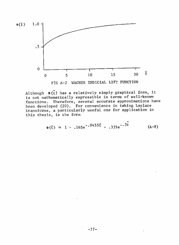
Wagner indicial function
Kussner indicial function
frequency
)F flutter frequency
(h' 'ca typical-section uncoupled frequencies,
h (Ch/m) , (Ca/la)
hl ,.al, modal uncoupled frequencies
Oh2,oa2 (Chl/m) , (Cal/Ia) , (Ch2/m) , (Ca2/Ia)
8(y) dirac delta function
A denominator in elements of two-mode,open-loop dynamics matrix, see Appendix D
X vector of lagrange multipliers
e observability matrix
X characteristic equation of typical section,uc = 0
XK characteristic equation of controlledtypical section
f(s) Laplace transform of i(t), s4(s)
-xiii-
I. INTRODUCTION
1.1 Background
Flutter can be defined as a self-excited, oscillatoryinstability of an elastic body in an airstream. Physically,this instability can occur when energy from the airstream
is absorbed by the body more rapidly than it is dissipatedby damping. The onset of the phenomenon is typically char-acterized by 'a flutter frequency and a critical airstream
speed. Flight at airspeeds in excess of this critical flut-ter speed can result in catastrophic structural failure.The problem of increasing the flutter speed of particularconfigurations has in the past been generally solved at theexpense of increased structural weight, through structural
modification and mass balancing, or by reducing aerodynamicefficiency, through geometry changes. Weight penalties inthe range of 10 to 25,000 pounds, for example, have beenestimated (1,2) to meet flutter requirements in SST classvehicles.
In more recent years, a substantial amount of experiencehas been obtained in developing active control systems forgust alleviation and the suppression of low frequency, in-sufficiently damped structural modes of an aircraft. Refs.
3 and 4 are excellent survey papers of the work done in these
areas. This experience, coupled with the potential perfor-
mance payoffs available (1-5), has made the active suppres-sion of the unstable flutter modes both feasible and desir-
able. Much of the work done in this latter area has occurredin the last 5 years, and some recent studies can be found inRefs. 6 through 11. In Ref. 6 a study, including analog sim-ulation and wind tunnel tests, was done using an unswept,symmetric wing model to determine the basic characteristicsof an active flutter control system. A simple aeroelasticmodel consisting of a cantilever plate with a follower forceat its free end was analyzed both experimentally and theore-tically in attempting to actively control flutter in Refs. 7and 8. Analytical analyses of more complicated structuralmodels applicable to the B-52 and F-4 respectively are des-cribed in Refs. 9 and 10, and in Ref. 11 a control systemdesign based on aerodynamic energy is discussed. Each ofthese analyses, though detailed in many respects, consideredrather simple sets of feedback parameters in designing theircontrol systems. This approach, dictated primarily by sensorcapabilities, ignores the possibility of using observors orestimators in determining unsensed parameters. The analyseshave, therefore, been severely limited in a number of respects:
-1-
(1) the maximum available increase in flutter velocity witha particular set of controllers can be limited, (2) deter-mining the gain values that produce this maximum flutter ve-locity increase can be tedious for complex systems, (3) se-lecting a control system design giving a particular fluttervelocity increase while optimizing other pertinent designparameters is difficult, and (4) design procedures cannot beeasily adapted to multi-input/multi-output systems. To re-move some of these limitations, this thesis incorporatesthree goals:
(a) Develop and demonstrate organized synthesis techni-ques for the design of flutter suppression systemsusing concepts of modern control theory
(b) Using a control moment gyro as the primary controltorque generator, indicate and illustrate designtradeoffs associated with the general developmentof a practical flutter suppression system
(c) Establish and identify attractive design featuresof the control moment gyro to warrant its consider-ation as a viable alternative to aerodynamic sur-faces in producing control forces to suppress flut-ter modes.
1.2 Control Moment Gyro
Although not usually mentioned when possible methods foractive flutter suppression are considered (4, 12), substantialexperience has been obtained using control moment gyros (CMGs)for momentum exchange in the attitude control of space vehiclesand satellites (13 - 19). To familiarize the reader with thistype of control, the following is a brief description of theCMG, including some of the possible advantages to be obtainedby its incorporation in a flutter suppression system.
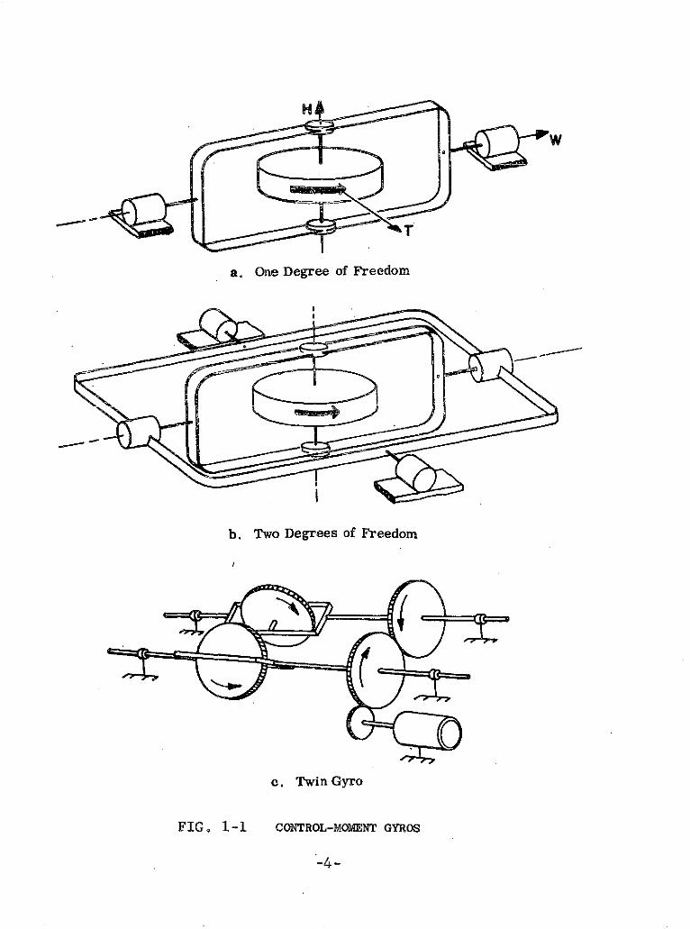
The CMG consists basically of a rotor (or wheel) witha known constant magnitude of angular momentum, and a methodby which the rotor can be precessed. As discussed more thor-oughly in Ref. 18, the three basic configurations for theCMG are, as shown in Fig. 1-1, the one-degree-of-freedom, thetwo-degrees-of-freedom, and the twin gyro. The one- and two-degrees-of-freedom gyros consist of one rotor mounted so thatit can be precessed about one or two axes respectively. These
-2-
systems, however, can have undesirable cross-coupling torques.The twin gyro consists of two counter-rotating gyro elementswhich are precessed through equal but opposite angles so thatthe control torque is always directed about a single axis.In a three-dimensional flutter analysis, the possibility doesexist that cross-coupling torques occurring for the one degree-of-freedom gyro could be used to advantage. However, theirinclusion in the flutter analysis introduces nonlinear termsinto the equations of motion. Therefore to maintain linearitythe twin-gyro control system will be used.
For space vehicle and satellite attitude control appli-cations, the control moment gyro has been shown to have ad-vantages in power, accuracy, response, and simplicity com-pared to reaction-wheel systems (16). Since output torqueis proportional to input gimbal rate, the CMG can producelarge moments on the airfoil at the relatively high flutterfrequencies without requirements for large angular momenta,and hence, large size. The effectiveness is not influencedby the complex aerodynamic forces which depend upon Machnumber and unsteady aerodynamic effects. Consequently, themathematical complexities in the analysis are somewhat reduced.Furthermore, the inherent lag in the development of forces onaerodynamic surfaces does not occur with this system,which should result in a reduction in the amount of lead ne-cessary for control and higher allowable controller bandwidth.Also, deflection angle of the' gyro gimbal is an easily meas-ured quantity and can be used directly as a feedback param-eter and in estimating other states of the system.
1.3 Thesis Summary
In Chapter II, the equations of motion for the typicalsection (two-dimensional wing surface) and CMG controllerare developed. Incompressible flow is assumed and the un-steady aerodynamics for arbitrary motion are represented byutilizing the Wagner indicial function. The open-loop char-acteristics of the system are examined with critical designparameters identified.
In Chapter III, the closed-loop characteristics of thesystem developed in Chapter II are determined. The system isplaced in standard state variable form with the definition oftwo new states, and the controllability and observability ofthe system are discussed. Full state and reduced state feed-back designs for various CMG sizes are determined.
-3-
a. One Degree of Freedom
b. Two Degrees of Freedom
c. Twin Gyro
FIG. 1-1 CONTROL-MOMENT GYROS
-4-
In Chapter IV, optimum feedback systems based on a num-ber of design criteria are determined. System response togust inputs is also calculated.
In Chapter V, the equations of motion for a three dimen-sional, uniform cantilever wing are developed using assumedmode methods. Optimum orientation and location of the CMGon the wing are determined. The open loop characteristicsof the system are calculated and comparisons are made withthe two dimensional analysis.
In Chapter VI, the closed loop characteristics of thesystem are examined including a discussion of the effectson controllability and observability of increasing the num-ber of vibrational modes in the analysis. Critical gains infull state feedback systems are identified, and a number ofreduced state systems are determined. The problem of highermode instabilities induced by the control is analyzed andmethods for reducing the probability of its occurrence arediscussed.
Chapter VII presents a summary of results, conclusions,and areas of further research.
-5-
II. TYPICAL SECTION WITH CMG:OPEN LOOP CONTROL CHARACTERISTICS
2.1 Wing-Controller Equations of Motion
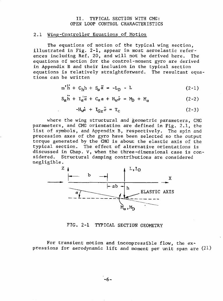
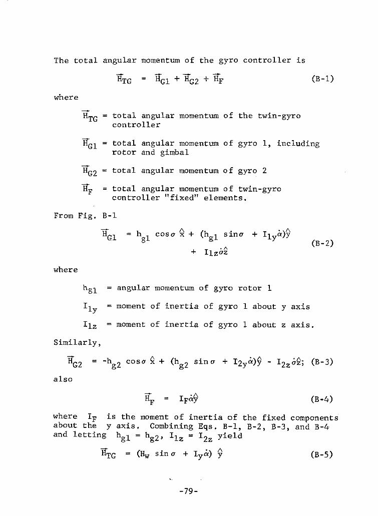
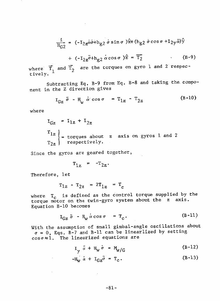
The equations of motion of the typical wing section,illustrated in Fig. 2-1, appear in most aeroelastic refer-ences including Ref. 20, and will not be derived here. Theequations of motion for the control-moment gyro are derivedin Appendix B and their inclusion in the typical sectionequations is relatively straightforward. The resultant equa-tions can be written
m'h + Chh + Sh' = -LD - L (2-1)
Sah + I a a + Ca a + Hw = I + Ma (2-2)
-Hu + IGz = Tc (2-3)
where the wing structural and geometric parameters, CMGparameters, and CMG orientation are defined in Fig. 2.1, thelist of symbols, and Appendix B, respectively. The spin andprecession axes of the gyro have been selected so the outputtorque generated by the CMG is about the elastic axis of thetypical section. The effect of alternative orientations isdiscussed in Chap. V, when the three-dimensional case is con-sidered. Structural damping contributions are considerednegligible.
Z L,LD
b I X
--ab ha ELASTIC AXIS
Ma, MD
FIG. 2-1 TYPICAL SECTION GEOMETRY
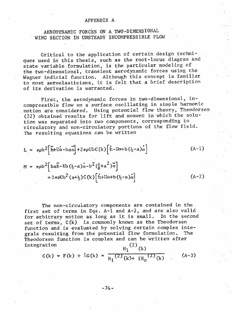
For transient motion and incompressible flow, the ex-pressions for aerodynamic lift and moment per unit span are (21)
-6-
L = pb2[h + Ua - baai] (2-4)
+ 2npbU J [~h(~) + Ua(E ) + b( -a)a (E)]4( r - )d
Ma n pb2[bah - Ub( - a)a - b 2 (1/8+ a2)i] (2-5)
+ 2 upb2U( + a) _d [h(-)+Ua(E)+b( -a)&(E), (r--)dEdt
where t = Ut/b is a dimensionless time measured in semi-
chords traveled after the start of the motion at t = 0. The
superscript dots, however, denote the derivative with respectto physical time, t. s(E) is the Wagner indicial admittance
function describing the circulatory lift buildup after a
sudden change in incidence, and is discussed in Appendix A.
Substituting Eqs. 3-4 and 2-5 into 2-1 and 2-2, and then
dividing Eq. 2-1 by npb and Eq. 2-2 by npb 4 produce the equa-tions
+ 1 K + h + (xa - a)a UT h bb
+-2 r rt +U a +( -a)'al(r - fDdt =-LD.+ 2 dr+ U-b J -tb b
(2-6)
(xaF - a) + 2 r. + ('/8+ a2)]a + U( - a)ab b
+ wra - 2 - ( + a)
x + Ua + ( -a)a l(r- T)d + Gloa = MD; (2-7)b b
-Gowoa + = c . (2-8)IGz
In order to simplify future operations with these equations,Eq. 2-6 is multiplied by (Q + a) and added to Eq. 2-7, whichyields
-7-
x, + ( + a) + ( + a) i-
2 1 U 22+ [xa( + a) + rap + (-a) a + 4 + ra~2aa + Glia& = 0.
Equations 2-6, 2-7a, and 2-8 are then the equations of motion
for the wing-controller system.
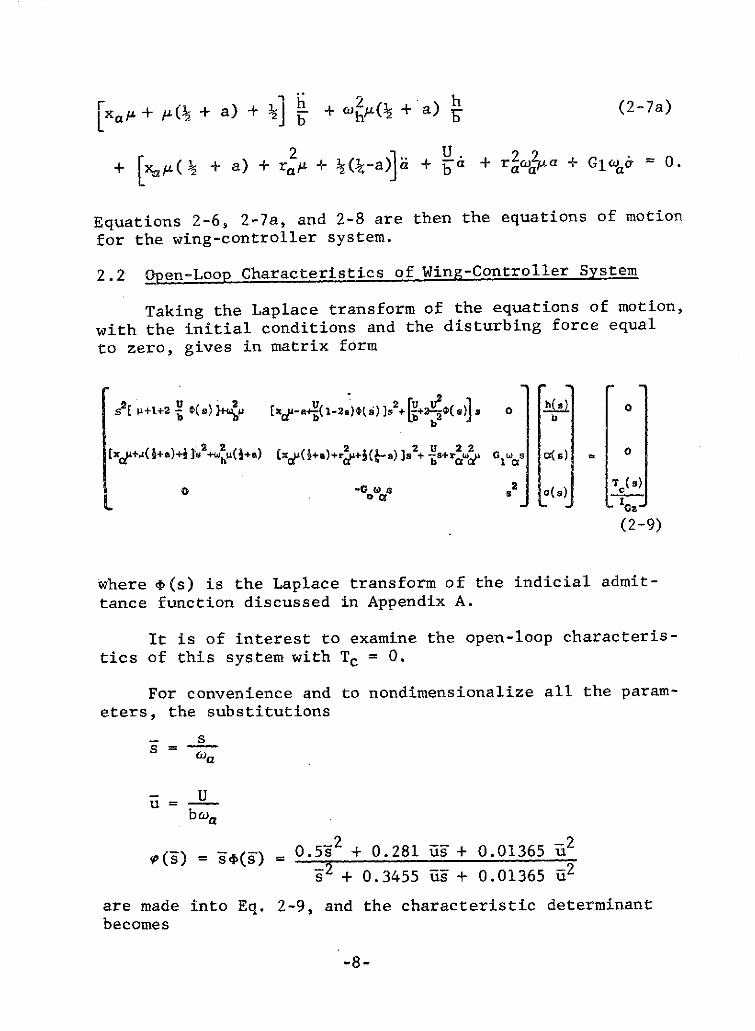
2.2 Open-Loop Characteristics of Wing-Controller System
Taking the Laplace transform of the equations of motion,with the initial conditions and the disturbing force equalto zero, gives in matrix form
s[ p+1+2 O (S) w [Xab 2)*() ]S2+yo U2 s) o
(xz&+40(+a)+is +w(j+S) [e )+ S) I S a+s)+crs+s1+ra) 0
0 -G 21 (s) T (s)
L Gz
(2-9)
where s(s) is the Laplace transform of the indicial admit-
tance function discussed in Appendix A.
It is of interest to examine the open-loop characteris-tics of this system with Tc = 0.
For convenience and to nondimensionalize all the param-eters, the substitutions
S =-
bOa
2 2(P) 0 .() = 0 2.5 + 0.281 U9 + 0.01365 2
S2 + 0.3455 us + 0.01365 G2
are made into Eq. 2-9, and the characteristic determinantbecomes
-8-
2
+2 2+ -(aW+ r +(1- a) P 9 ;+2 i! G) =
0 2 (2-10)
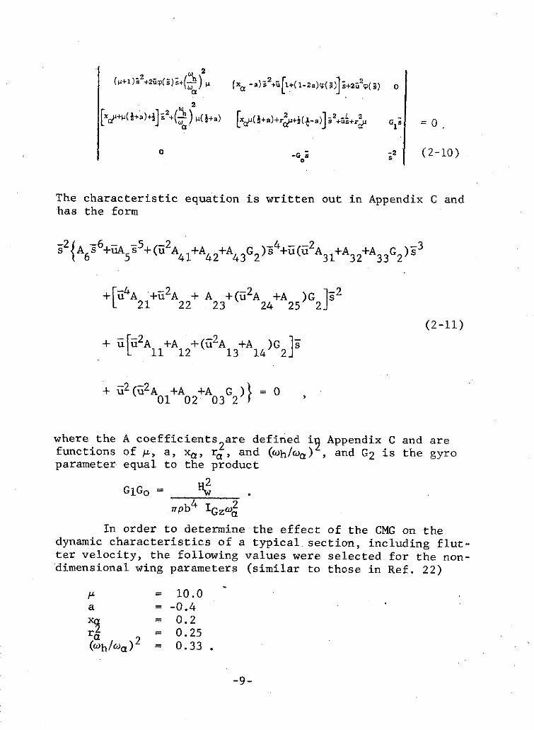
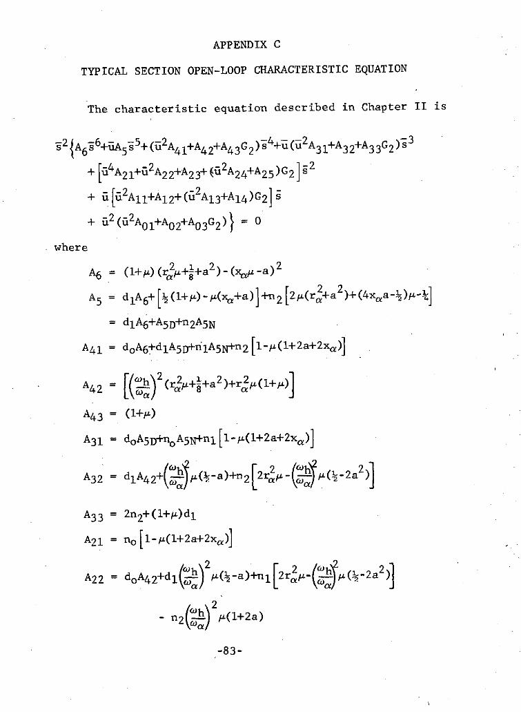
The characteristic equation is written out in Appendix C andhas the form
s2 {A6 g6+ A 5 s 2+( A41+A42+A43G2)4 + (u2A3 1+A32+A33 G 2 ) 3
where the A coefficients2 are defined i Appendix C and arefunctions of 4, a, xa, ra, and (Oh/owa) , and G2 is the gyroparameter equal to the product
GlG o =
npb4 IGz
In order to determine the effect of the CMG on thedynamic characteristics of a typical section, including flut-ter velocity, the following values were selected for the non-dimensional wing parameters (similar to those in Ref. 22)
FL = 10.0a = -0.4x = 0.2r= 0.25
(wh/wa)2 = 0.33 .
-9-
S ubstituting these values into Eq. 2-11 yields
2 24.88.6+15.97 - 5+(0.36U 2+36.67+11.0 G2) 4
+ ui(-1.31 u2+17.84+4.8 G2)s 3
+ [-0.40 u4+2.76u2+8.25+(0.71l2+3.3)G 2] 2
+ u [-0o.085s2+2.8+(0.006u2+l.14)G2 s
+ i2[ -0.009u2+0.113+0.045 G2]
= 0.
(2-12)
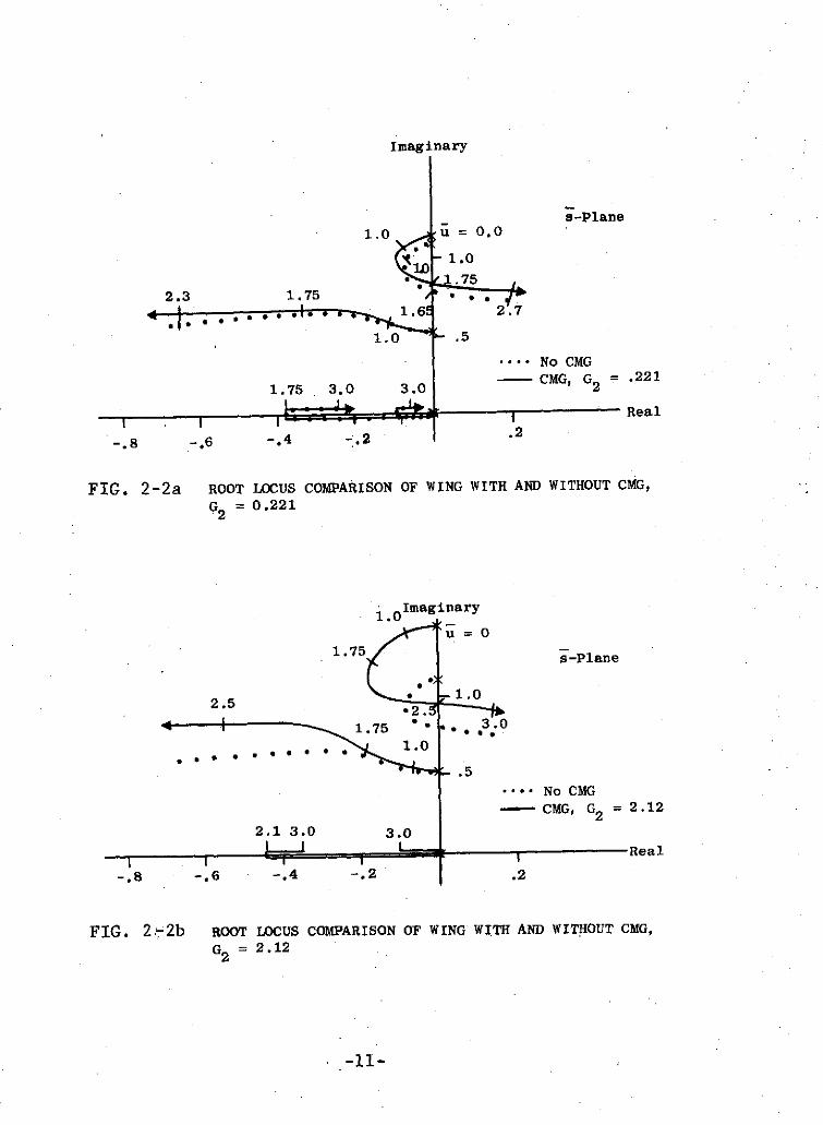
Figures 2-2a and 2-2b show a comparison of the rootloci for this system for three values of G2 including G2 = 0,i.e., without CMG. The root loci are drawn for variationsof the velocity parameter u = U/bwa, which will imply, inthis analysis, variations in U with oa and b held constant.Roots marked "x" indicate u = 0. From the figures, it canbe seen that for the particular values chosen for the non-dimensional parameters, the critical roots associated withthe onset of flutter correspond to the torsion branch of theroot locus plot. The frequencies associated with the bending-torsion modes approach one another as the flutter velocity isapproached for each case, which is a result often occurringin classical bending-torsion flutter. For increasing valuesof U beyond its flutter value, the frequencies correspondingto the bending and torsion branches of the root locus tendto converge to the same value. The roots that remain fixedat the origin for varying u are associated with presence ofthe CMG in the system.
For increasing values of G2, corresponding increases influtter velocity and flutter frequency occur. This can beseen more explicitly in Fig. 2.3 which shows that increasingG2 from 0.0 to 5.0 results in increases for uF from 1.65 to3.35 and for wF/wa from 0.80 to 1.11. In general, increasesin the value of G2 would correspond to increasing the size ofthe CMG. However, for a constant value of angular momentum,increasing G2 could correspond to a decreasing value of IGzwith fixed angular momentum, which would be associated witha decreasing CMG size.
-10-
Imaginary
s-Plane1.0 u =0.0
1.0
* .752.3 1.75 .
. ' • 1.6 2.7
1.0 .5
.... No CMG
1.75 3.0 3.0 -- CMG, G2 = .221
Real
.2-. 8 -. 6 -,4 -. 2 .2
FIG. 2-2a ROOT LOCUS COMPARISON OF WING WITH AND WITHOUT CMG,
G2 = 0.221
.O Imaginary
u 0
.75 s-Plane
S. 1.02.5.
-1* No CMG---- CMG, G2 = 2.12
2.1 3.0 3.0
-.8 -.6 -.4 -.2 .2
FIG. 272b ROOT LOCUS COMPARISON OF WING WITH AND WITHOUT CMG,G2 = 2.12
-12-
UF
wF -4.0
-1.5 - 3.0
-1.0 2. ,
- , Flutter Velocity
-.5 -1.0 wS, Frequency at Flutter
o I I I I I0.0 1.0 2.0 3.0 4.0 5.0
H2
wG2 -b4 2 Gyro Parameter
itpb I wGz a
FIG. 2-3 VARIATION IN VELOCITY AND FREQUENCY AT FLUTTERWITH G2
-12-
In the next chapter, the effect of feedback on this sys-
tem will be examined.
-13-
III. FEEDBACK CONTROL OF TWO DIMENSIONALWING-CONTROLLER SYSTEM
3.1 State Variable Formulation
The characteristic equation developed in the previoussection is 8th degree, where the two roots located at theorigin in Figs. 2-2a and 2-2b are associated with the pres-
ence of the CMG in the system. If feedback of the gimbalangle a were not required, the degree of the characteristicequation could be reduced to seven. However, passive oractive feedback of gimbal angle is necessary to maintain thevalidity of the small-gimbal-angle assumption in the equa-tions of motion. Thus, the minimum number of states to de-fine this system is eight. It would be advantageous forsensor and estimator design requirements if it were not nec-essary to obtain information on all states to adequatelysuppress the onset of flutter for reasonable increases inthe velocity. To obtain some insight into which parametersare most significant in the control law, an analysis usingarbitrary dynamics is done in this section. In this method,the eigenvalues of the uncontrolled system are shifted toarbitrary new locations using state variable feedback. Thisrequires that the system be modally controllable with theparticular set of states chosen to define the system. Todetermine the controllability of the system, the equationsof motion (Eqs. 2-6, 2-7a, 2-8) are first put into standardstate-variable matrix form, which can be written in general,with no disturbing forces
x = Fx + Gc (3-1)
where x is the state vector and gW the control vector. With,(§)= N./D., the first equation in Eqs. 2-9 is multipliedby D,, and then the inverse Laplace transformation of Eqs.2.9 is taken assuming zero initial conditions. The result-ing equations can be written
B + (Bldl + 1)h (Bld2 + 2u 2 n I + B )lb 1 4)b
+ [2nou3 + B4dlu] - + B4 d 2U + B2 I8 + u(B 2 dl+ B3 n 2+ 1)
Equations 3-2 are equivalent to Eqs. 2-6, 2-7a, and 2-8 in-
sofar as they have the same characteristic equation. For
certain nonzero initial conditions, the dynamic response of
the two systems would be different.
Before writing Eqs. 3-2 in standard form, a decisionmust be made as to which quantities are considered states.
There are many possible realizations of the system of equa-tions, and the procedure here will be to select those stateswhich would be the least complicated to individually sense,and can be explicitly identified. The following quantitiesare therefore selected as the states of the system:
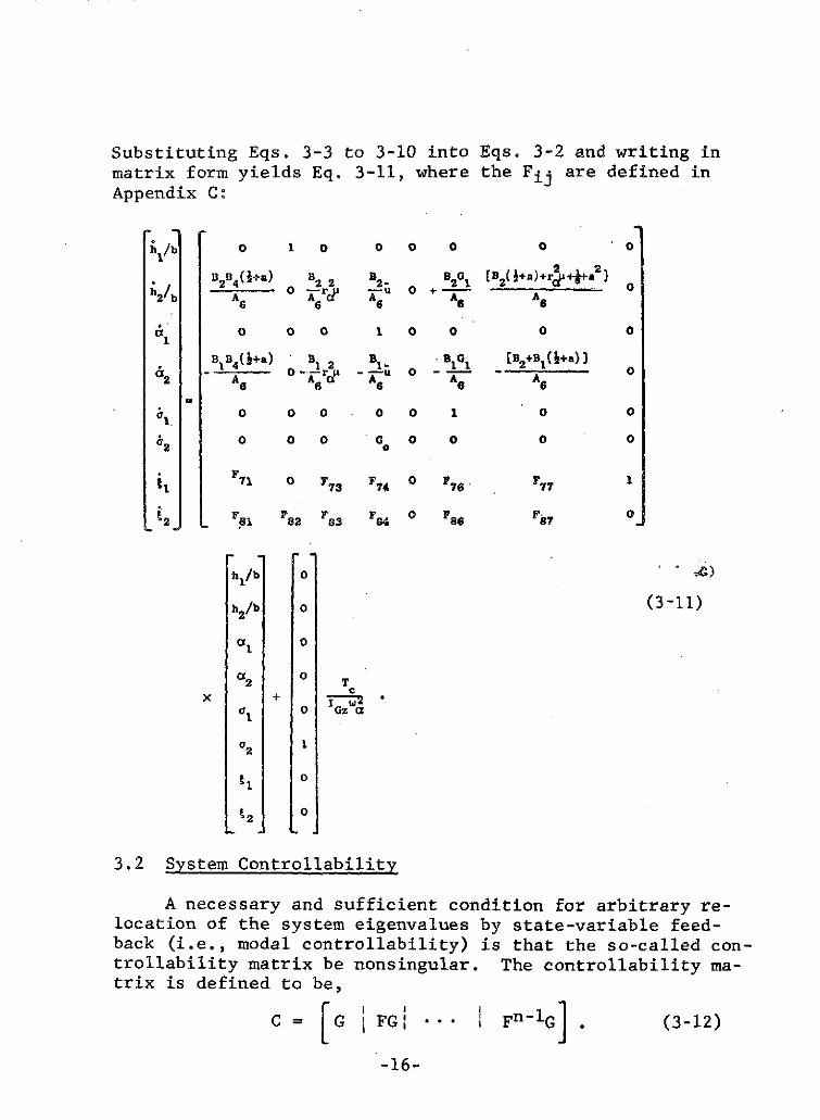
Substituting Eqs. 3-3 to 3-10 into Eqs. 3-2 and writing inmatrix form yields Eq. 3-11, where the Fij are defined inAppendix C:
£hI/b 0 1 0 0 0 0 0 0
S 2 B 4(i+a) B2 2 2- B2G [B2(i+a)+r4++ 2 ]- 0 +- 0
'2/b A O 6 A A Aa
Et1 0 0 0 1 0 0 0 0
S B1 4 ( J+a) 81 2 - 810 [(2+B1 (+a
) ]
A 06 Ag A6
l 0 0 0 0 0 1 0 0
2 0 0 0 G° 0 0 0 02 o
i 71 0 773 F4 0 F76. F77
2 F a F82 F F 0 F as F87 02 81 82 F83 84 6 87 0
ri 1
h1 /b 0
h2 /b 0 (3-11)
a oX2 0 T
x + - C
0 1 0 Gz a
02 1
t2 0
3.2 System Controllability
A necessary and sufficient condition for arbitrary re-location of the system eigenvalues by state-variable feed-back (i.e., modal controllability) is that the so-called con-trollability matrix be nonsingular. The controllability ma-trix is defined to be,
C = G i FG ** Fn -1G . (3-12)
-16-
where n is the number of states defining the system. It canbe shown that this matrix is nonsingular for the parametersselected in this analysis with Gl, Go > 0 , U > 0.
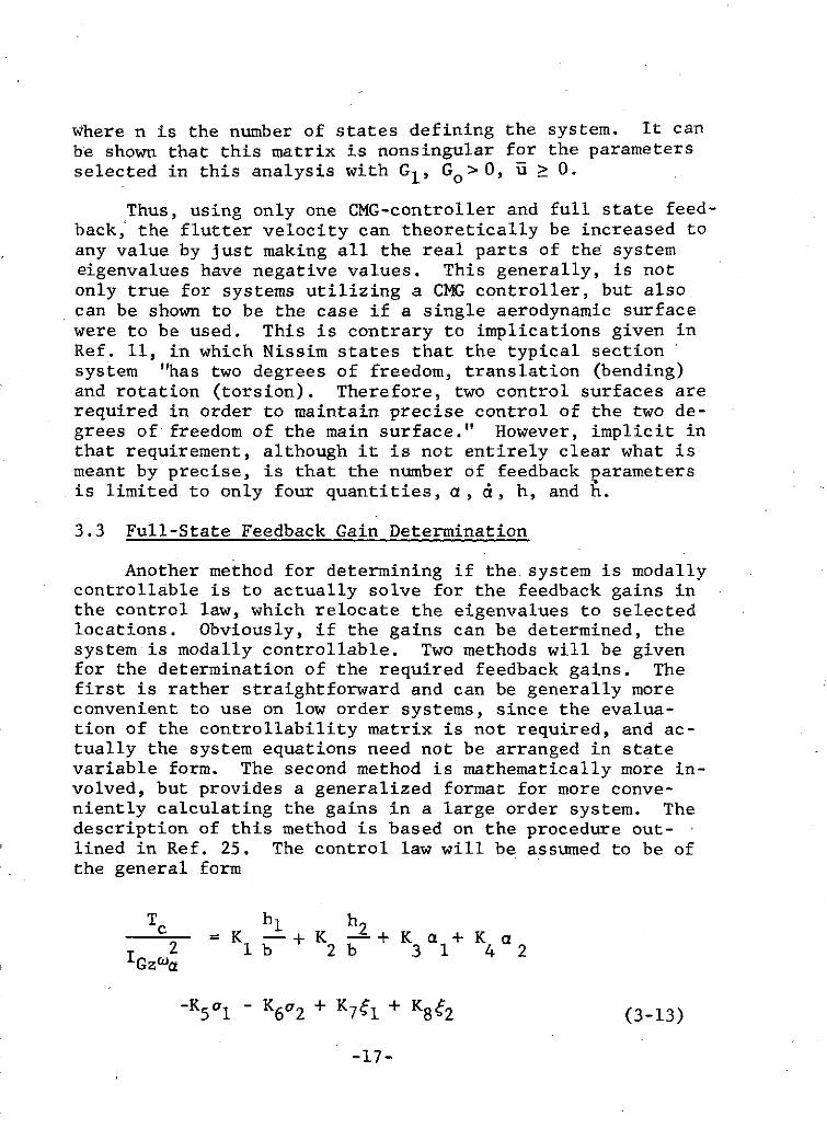
Thus, using only one CMG-controller and full state feed-back, the flutter velocity can theoretically be increased toany value by just making all the real parts of the systemeigenvalues have negative values. This generally, is notonly true for systems utilizing a CMG controller, but alsocan be shown to be the case if a single aerodynamic surfacewere to be used. This is contrary to implications given inRef. 11, in which Nissim states that the typical sectionsystem "has two degrees of freedom, translation (bending)and rotation (torsion). Therefore, two control surfaces arerequired in order to maintain precise control of the two de-grees of freedom of the main surface." However, implicit inthat requirement, although it is not entirely clear what ismeant by precise, is that the number of feedback parametersis limited to only four quantities, a, d, h, and h.
3.3 Full-State Feedback Gain Determination
Another method for determining if the system is modallycontrollable is to actually solve for the feedback gains inthe control law, which relocate the eigenvalues to selectedlocations. Obviously, if the gains can be determined, thesystem is modally controllable. Two methods will be givenfor the determination of the required feedback gains. Thefirst is rather straightforward and can be generally moreconvenient to use on low order systems, since the evalua-tion of the controllability matrix is not required, and ac-tually the system equations need not be arranged in statevariable form. The second method is mathematically more in-volved, but provides a generalized format for more conve-niently calculating the gains in a large order system. Thedescription of this method is based on the procedure out-lined in Ref. 25. The control law will be assumed to be ofthe general form
T b h= K -+ K -+ K a + Ka2 lb 2b 3 1 4 2
IGzla
-K 5al - Kg2 + K751 + Kgi2 (3-13)
-17-
or in vector notation
T T
Gz a h2aI
a 2al
a 2
e152
(3-14)
The basic problem of selecting gains to arbitrarilyplace the system eigenvalues can be stated as follows:
Given the single-input system
x = Fx + guc (3-15)
(where for application to Eq. 3-11, u c is a scalar and & isa vector) with the characteristic polynomial for uc = 0,
X(s) = det (sI-F) = s n +f 1 sn-1+ ..... fn, (3-16)
find the gain vector K such that the characteristic polyno-mial of the system
= (F - gKT)x (3-17)
has the specified form
XK(s) = sn + g1 sn-l ........ gn . (3-18)
Whenever the system contains a small number of states,a solution for the gains can sometimes be generated more
-18-
conveniently by directly expanding the characteristic deter-minant of Eq. 3-16 and equating the coefficients of likepowers of s with those of the desired characteristic equa-tion, Eq. 3-18. For example, for the particular system des-cribed in Eq. 3-11, a solution can be developed by substitutingthe Laplace transform of Eq. 3-13 into the transform of Eq.3-2 which results in the following characteristic determi-nant:
1 i4 + r(B d +l)3 + B do+2n )2+B4 2 B2 4 + (B2d l++B3n2 3 O
+ (23no +B4d 1 ) + B4 do2
+ (B2do+d +B3n +1)2 2
+(do+B3n+2n )B3 + 2n U4
2r 2 =)2 2 K
[B2 + + a)] 2 + B4(j + a) 82(4-a)+r -+ a 2 + s + rXK2 1Ba, 2)+rCr±a G K'
Expanding this determinant and equating coefficients estab-lishes eight equations, which can be solved simultaneouslyfor the eight gains to arbitrarily relocate the eigenvaluesof the system.
For large order systems the above approach could betedious, and a procedure more amenable to computerized solu-tion is needed. The following method is presented from Ref.25. From Eq. 3-17
XK(s) = det (sI - F + KT )
= det (sI - F)(I + (sI - F)-1 g IT)
= det (sI - F)'det (I + (sI - F)-l KT)
= X(s)' (1 + KT(sI - F)-1 K) (3-20)
-19-
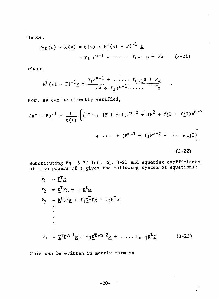
Hence,
YK(s) - X(s) = X(s) * KT(sI - F) - 1
= Yl sn-1 + ...... Yn-l s + Yn (3-21)
where
1 s n - 1 + ...... Yn- 1S + YKT (sI - F) = n-sn + fls ...... n
Now, as can be directly verified,
(s F)- 1 n - + (F + fll)sn-2 + (F 2 + fl F + f21)s n - 3
+ .... + (-1 + flFn- 2 + ... _fn-1)
(3-22)
Substituting Eq. 3-22 into Eq. 3-21 and equating coefficients
of like powers of s gives the following system of equations:
Y = KT g
Y2 = KTF + fKT g
Y3 = KTF 2 + flKTF + f 2KT&
Yn = KTFn-lg + flKTFn-2 &+ ..... fn-1& (323)
This can be written in matrix form as
-20-
T T
fl KTF& gTFT
Y= f2 fl 1 =R K
2 • .
fn-1 ..... f2 fl I KTFn-1 TFT(n-)
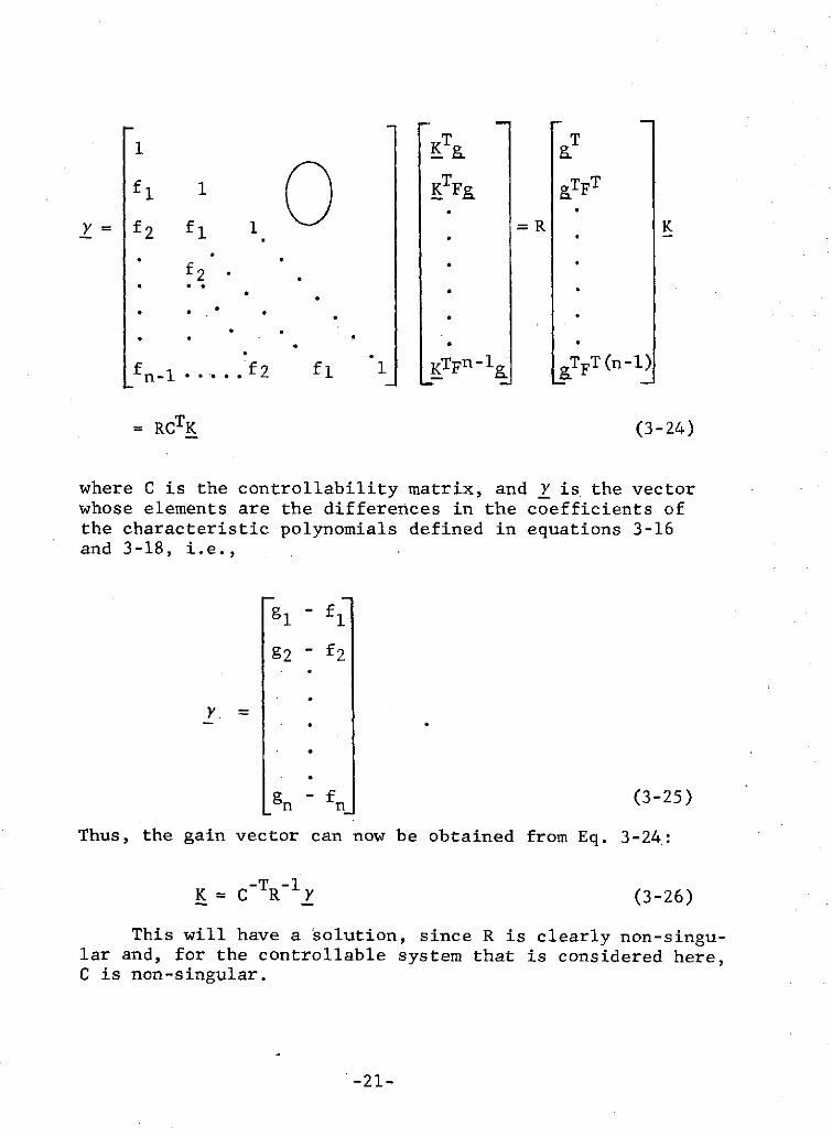
= RCTK (3-24)
where C is the controllability matrix, and Y is the vectorwhose elements are the differences in the coefficients ofthe characteristic polynomials defined in equations 3-16and 3-18, i.e.,
f 1
g2 f2
gn -fn (3-25)
Thus, the gain vector can now be obtained from Eq. 3-24:
K = C-TR- Y (3-26)
This will have a 'solution, since R is clearly non-singu-lar and, for the controllable system that is considered here,C is non-singular.
-21-
3.4 Design by Arbitrary Dynamics (Pole Placement)
An extensive parametric study was done, utilizing equa-tions obtained from Eq. 3-19, in order to determine some of the
characteristics of the wing-controller system. Variations in
U, G2, and root locations were considered. Although later de-
sign specifications may dictate additional requirements on the
root locations, the one stability criterion established for
arbitrary root placement was that the minimum negative value of
the real part of any root would be greater than 0.05%a when U
is greater than its critical value for the wing without the
CMG (i.e., _ > 1.65). Consequently, two particular situations
arose in the analysis, depending on the values of G2 and i:
(1) one conjugate pair of roots had positive real parts or did
not meet the stability criterion, and thus, to maintain an
adequate stability level, these roots plus the two roots at
the origin (Fig. 2-2) had to be relocated by proper selection
of the control gains; (2) all roots except those at the origin
met the stability criterion, with no positive real roots. The
roots that are relocated in order to meet the stability crit-
erion will be referred to as the critical roots. When judging
the merits of various root locations for particular values of
G2 and u, the relative size of each set of control gains wasthe basis of comparison, with smaller gains implying a moredesireable design. Though not a direct indication of the qual-ity of a particular design, the size of the gains do providea measure of the relative minimum values of the torque and
power requirements among designs constrained to the same stab-ility criterion. This is verified by the results of Chap. 4.Low gain values also facilitate the determination of adequatereduced feedback systems, since elimination of certain feed-backs as unnecessary can be made when their values are negli-gible. The following results and conclusions were obtainedfrom the parametric analysis
a. The lowest gain values are obtained when only the crit-ical roots are relocated and are placed as near to theimaginary axis as allowed by the stability criterion.
b. When relocating only the roots at the origin, thevalues of the gains are reduced by placing the rootson the real axis.
c. When there are four critical roots, the gain valuescan be reduced (1) by proper adjustment of the imag-inary part of roots originally located at the origin,
-22-
and (2) by relocating the torsion-branch roots atapproximately the same distance from the origin asthey were with no control.
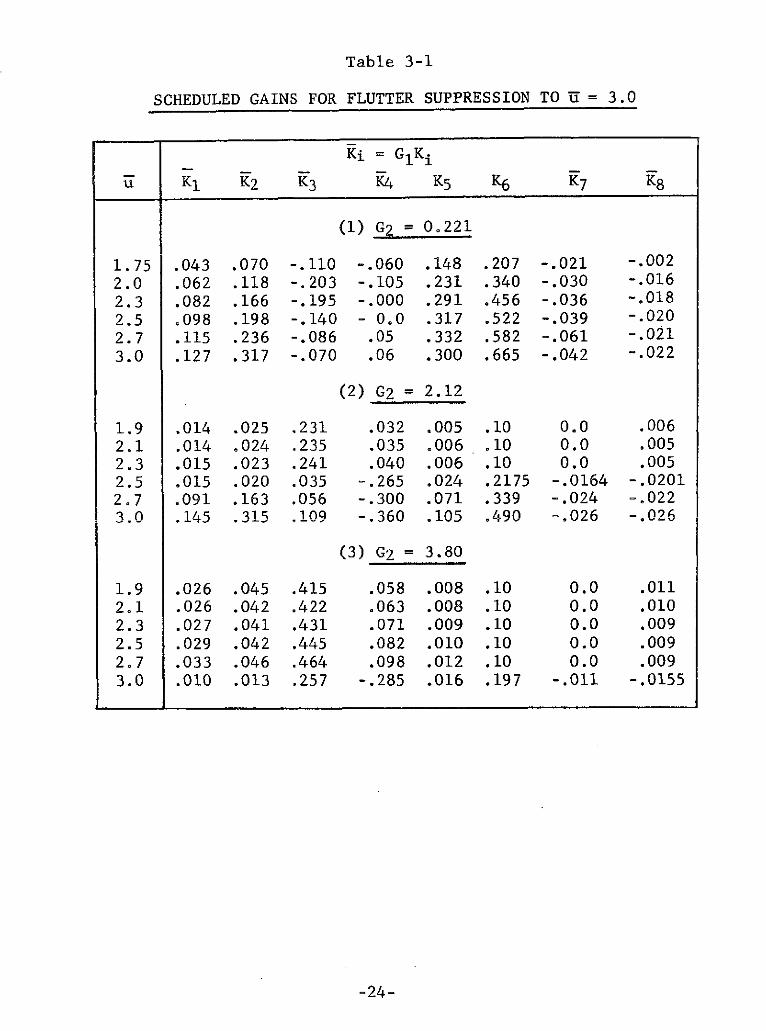
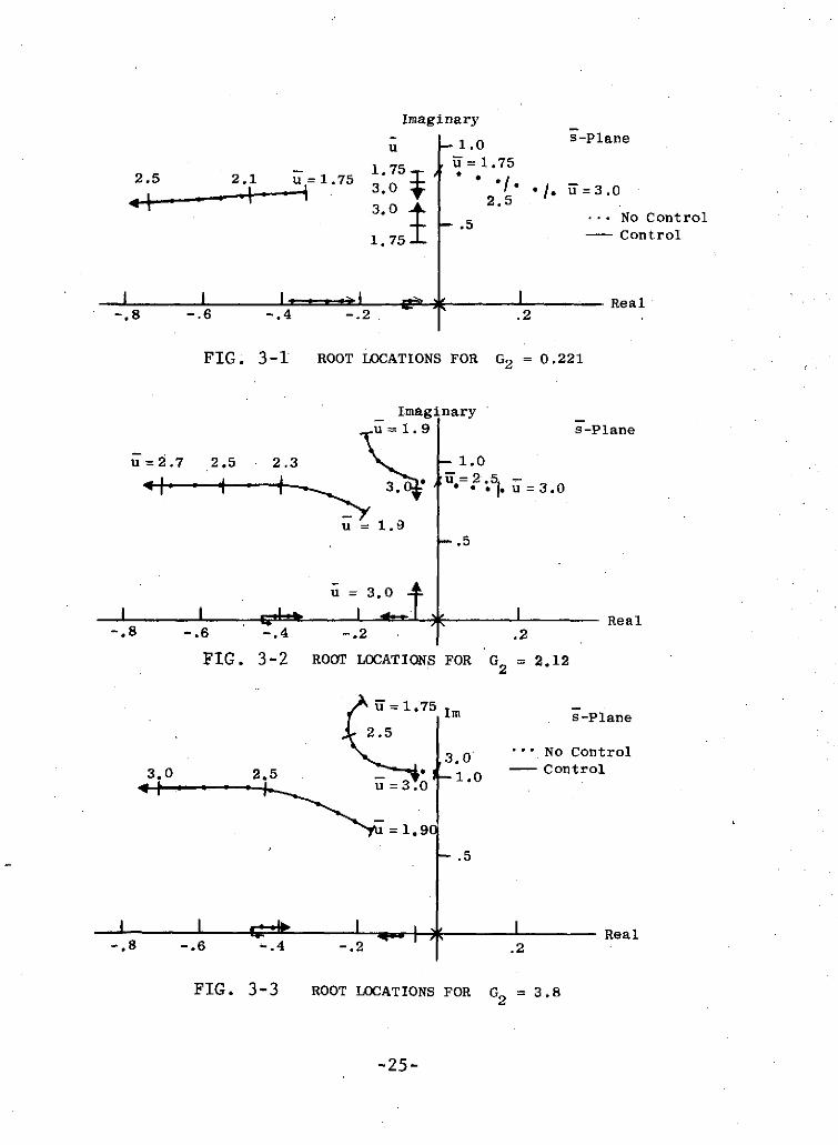
d. Gain scheduling, in which the gains are made afunction of freestream velocity, can be used toreduce the gain values over a range of veloc-ities. Depending on the value of G2, all the gainsneed not be scheduled, but even with reduced sched-uling, the added complexity may be prohibitive fora particular design. The following three examplesillustrate the effects of gain scheduling. Sincethe wing is stable without the CMG for U < 1.65,only the feedback characteristics for U > 1.65 wereconsidered of interest.
Table 3-1 shows, as a function of velocity and forthree values of G2, the gains needed to place theeigenvalues of the system at the desired new loca-tions as shown in Figs. 3-1, 3-2, and 3-3. Theroot locations were chosen to produce minimum gainvalues using the guidelines indicated above in a,b, and c. In the characteristic equation, all the
gains except K5 and K6 appear multiplied by thegyro term, G1 . Thus in Table 3-1, Ri
= GlKi isused as a convenient parameter to describe thefeedback characteristics, since, for a given G2and set of root locations, Ki will remain constantfor variations in Gl and Go . Figures 3-1 to 3-3show three different control situations:
(1) G2 = 0.221: There are four critical rootsfor all i.
(2) G2 = 3.8: For each U except U = 3.0, onlytwo critical roots exist.
(3) G2 = 2.12: For U52.4 there are two criticalroots, and for U > 2.4 there are four criticalroots.
For G2 = 3.8, the gains remain relatively constantover the range of velocities considered except atU = 3.0. This indicates that a set of constantgains could be selected which would place the rootsin approximately the same locations. For G2 = 0.221,
-23-
Table 3-1
SCHEDULED GAINS FOR FLUTTER SUPPRESSION TO U = 3.0
each of the gains varies somewhat, with only feed-backs of h and having a significant variationwith velocity. For G2 = 2.12, each gain does showsignificant variation with velocity, caused pri-marily by the change from two to four criticalroots as the value of U increases beyond 2.4.
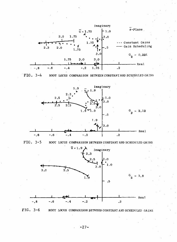
Figures 3-4, 3-5, and 3-6 show a comparison of theroot loci for G2 = 0.221, 2.12, and 3.8 respectively,using constant gains and gain scheduling. Figure3-6 shows that constant gains can be used with verylittle change in the root locus. Figure 3-4, G2 =0.221, shows that there is very little change inthe noncritical roots using constant gains. Thecritical roots become located on either side oftheir scheduled value, For G2 = 2.12, Fig. 3-5shows what differences may result when using con-stant gains. The roots corresponding to the torsionbranch of the root locus with constant gains followthe bending branch associated with scheduled gains,and the bending branch of the root locus with con-stant gains results in the critical flutter condi-tion.
Thus, it appears that to obtain the best resultsusing constant gains, the value of G2 should beselected to give an open-loop flutter velocitygreater than the maximum flutter velocity desiredfor a particular application.
e. Relaxing the stability criterion, such that thecritical roots can be placed nearer the imaginaryaxis, can result in reduced values for the gains.The size of the gains, however, may not provide anaccurate measure of the relative values of the torqueand power among designs constrained to differentstability criterion.
f. Although feedback of eight states is necessary toplace exactly the set of roots at a desired loca-tion for particular values of velocity and G2,adequate stability can be achieved with reduced-feedback systems. A number of possible designsusing various combinations of the feedback param-eters can be developed, depending on the values of
-26-
Imaginarys-Plane.
u = 1.75 -1.0
2.0 1.75 .0
1.75 *.. Constant Gains
2.3 2.0 1.75 --- Gain Scheduling
3.0 G2 = 0.221
1.75 3.0 3.0
I I IL I I Real
-.8 -.6 -.4 -.2 1.75 .2
FIG. 3-4 ROOT LOCUS COMPARISON BETWEEN CONSTANTAND SCHEDULED GAINS
Imaginary1.9 uu =1.9
2.3*2.5 ) 1.0
3.0
1.9
6I I - I I Real
-.8 -.6 -.4 -.2 .2
FIG. 3-5 ROOT LOCUS COMPARISON BETWEEN CONSTANT AND SCHEDULED GAINS
u=1.9Imaginary
2.3
2.5 3.0
3.0 1.0
3.0 2.5
G = 3.81.9 2
.5
Real
-.8 -.6 -.4 -.2 .2
FIG. 3-6 ROOT LOCUS COMPARISON BETWEEN CONSTANT AND SCHEDULED GAINS
-27-
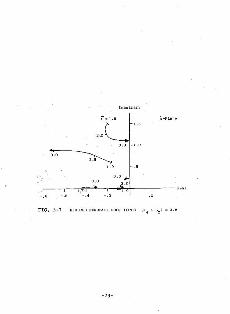
u, G2 and the eigenvalues of the system. One ex-ample of a reduced-feedback system can be obtainedfrom Table 3-1 for G2 = 3.8. The significant gainscorrespond to feedback of a and 6, and a designusing only these two feedbacks, along with a to nullthe gyro, results in a root locus very similar tothe eigenvalues shown in Fig. 3-6.
The simplest feedback system for any value of G2can be determined by examining the characteristicdeterminant, Eq. 3-19. It can be seen that feed-back of &(K4) has the same influence on the rootsin the characteristic equation as Go . Consequently,increasing the value of the gain parameter K4 isequivalent to increasing G2. Figure 3-7 showsthe root locus for a system using only two feed-backs characterized by the gains
(K4 + G2 ) = 3.8
K 5 = 0.10
For G2 = 3.8, this system reduces to one requiringthe feedback of only a.
A comparison of the response characteristics of thissystem with systems using all eight states as feed-backs will be done in Chap. 4.
3.5 System Observability
In the preceding analysis, total knowledge of all thenecessary states for use in the control laws was assumed.This information could be obtained through sensor measure-ments or through a properly designed estimator if it werenot possible or convenient to measure directly the desiredstates. The sensor problem would be reduced to a minimum ifall the states could be estimated from one measurement, themost convenient of which would be a. If the state of a sys-tem at any time can be uniquely determined by the availablemeasurements, the system is considered observable. The ob-servability of the wing-controller system, assuming only ais measured, can be qualitatively determined by examiningEqs. 3-2. Mathematically, observability can be determined
by the requirement that the observability matrix be non-singular. The observability matrix is defined to be
H
HF
HF n - 1 (3-27)
where H is the output matrix defined from
y = Hx (3-28)
and y is the measured quantity. With only a measured,
H = 0 0 0 0 1 0 0 0]. (3-29)
It can be shown that the observability matrix is non-singular for the parameters selected in this analysis forGo, GI > 0, U 0.
Thus, it appears a may be the only quantity necessaryto measure, since stability can be achieved with only a feed-back. If more control of the eigenvalue locations is desired,the other states can be estimated from this measurement.
-30-
IV. SYSTEM DESIGN USING OPTIMALCONTROL
4.1 Optimal Control Using Quadratic Synthesis
In Section 3.4, the relative values of the gains in
the control law were used as a basis for comparing various
eigenvalue locations. A criterion more directly associated
with system performance, which results in stable, linear
feedback control, can be obtained by minimizing a cost
function made up of integral quadratic forms in the state
and control. Determining the control requirements in this
case is basically similar to the optimal regulator problem
as discussed in Ref. 26. The following is a brief descrip-
tion of this method.
As has been shown previously, the equations of motion
can be written.in the form
x = Fx + Gu (4-1)
It is desired to minimize a cost function of the form
J 1_ I (xTAx + ucTBuc)dt (4-2)20
where superscript T indicates the matrix transpose, and A
and B are symmetric weighting matrices selected to obtain
"acceptable" levels of x and c. The control uc which
minimizes J can be obtained by solving Eq. 4-1 simultan-
eously with the Euler-Lagrange equations
iTC x (4-3)
Uc (4-4)
where
) = xTAx + ucTBc + AT (F + Gc)
and X is a vector of Lagrange multipliers.
-31-
Substituting for t in Eqs. 4-3 and 4-4 yields
S= - Ax - FTA (4-5)
U - B-lGTo (4-6)
Substituting Eq. 4-6 into 4-1 and combining with Eq. 4-5 gives
[ F -GB-1GT x= _ -F r (4-7)
-A -FT
One method of solving Eq. 4-7 is by using the substitutionA = Sx, where S is a matrix. This results for the regula-tor problem in determining the steady-state solution of amatrix Riccati equation for S of the form,
SF + FTS - STGB-lGTS + A = 0 (4-8)
The feedback gain matrix, K, in the control law uc = -Kxis then obtained from
K = B-lGTS. (4-9)
Another method of solution is by eigenvalue decomposition asdescribed in Ref. 27.
Obviously, critical to any solution of this problem isthe choice of weighting matrices. One "rule of thumb" inselecting A and B is to choose diagonal matrices whoseelements are equal to
1 and 1
(ximax)2 , (ucmax) 2
respectively, where ximax and ucmax are the maximum"acceptable" values of xi, the elements of state vector,and uc respectively. It must be remembered, of course,that the weighting matrices are only relative, and the actualmaximum values and their relative sizes occurring in practicewill depend on the system response to initial conditions anddisturbances.
-32-
As a first step in this introductory analysis, thediagonal elements of A are considered to be very small
with respect to B, so that no restrictions are placed on
the state behavior other than stability and therefore the
design that essentially minimizes U dt is beingdetermined. The matrix A can be positive semi-definite
to the extent that it cannot be identically zero, since, as
can be seen from Eq. 4-2, the solution degenerates to the
case, uc = 0.
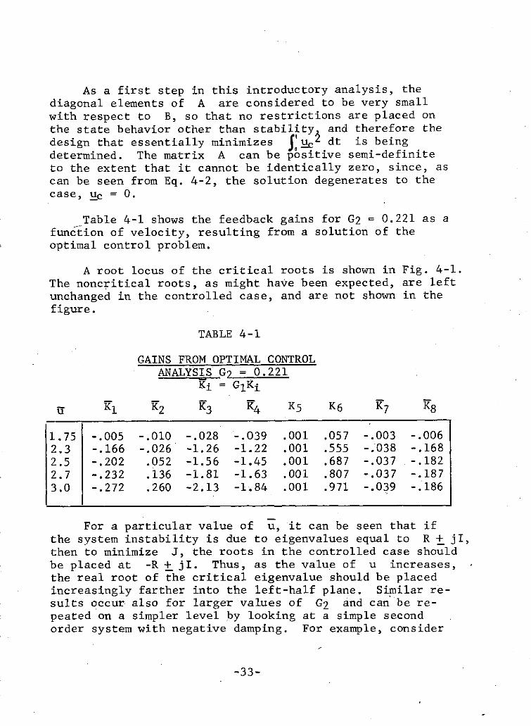
Table 4-1 shows the feedback gains for G2 = 0.221 as afunction of velocity, resulting from a solution of the
optimal control problem.
A root locus of the critical roots is shown in Fig. 4-1.
The noncritical roots, as might have been expected, are left
unchanged in the controlled case, and are not shown in the
For a particular value of u, it can be seen that if
the system instability is due to eigenvalues equal to R + jI,then to minimize J, the roots in the controlled case shouldbe placed at -R + jI. Thus, as the value of u increases,the real root of the critical eigenvalue should be placedincreasingly farther into the left-half plane. Similar re-sults occur also for larger values of G2 and can be re-peated on a simpler level by looking at a simple secondorder system with negative damping. For example, consider
-33-
Imaginary
s-Plane
1.03 2.3 1.75
u=3.0 2.3
.5
- Controlled Case... Uncontrolled Case x Roots Remain
Constant
I I I I Real
-.4 -.2 .2 .4
FIG. 4-1 ROOT LOCUS FROM OPTIMAL CONTROL ANALYSISG2 = 0.221
-34-
x 2Rx +x = UC.
For y, = 0, the eigenvalues are
s =R + jI
with
I = , 0- R 2
To minimize
J = (xTAx + bu)dt
with the diagonal elements of A small,
u a -4Rx.
The resulting eigenvalues are
s = -R + jI.
Since six of the eight roots remain essentially unchanged
in the higher-order system when going from the uncontrolled
to the controlled case, this system takes on characteristics
similar to those of a simple harmonic system.
The large gain values appearing in Table 4-1 as com-pared to those in Table 3-1 are in part due to the tighter
control requirements resulting from moving the pair of
critical roots farther into the left-half plane. Primarily,
however, the large values are due to the relocation of the
roots originally at the origin. It was found in Section 3.4
that proper placement of these roots can result in lower
gains (and for the particular value of G2 used in this
analysis, large gains result for placement of these roots
near the real axis). Thus, whether gain values can be used
to indicate a desirable design as was done in Section 3.4
depends on what particular function is being optimized.
Because of the placement of the critical roots in
achieving the minimum integrated value of control torque,the initial values of torque tend to be large. This feature
of the design can be partially alleviated by redesigning the
-35-
control for larger values of G2. In fact, for practicaldesign considerations, the maximum values of torque andpower may be more critical parameters than the time inte-gral of control torque. The effects on these parametersand other response characteristics resulting from variationsin u, G2 , and root locations are investigated in Section4.2.
4.2 System Response to Gust Impulse
The aerodynamic lift and moment produced by gust-likedisturbances in the airstream are a major source of externalloads on a lifting surface. The lift and moment distur-bances created by an impulsive upward gust striking theleading edge at time t = 0 can be described by (20)
LD = 2npbU2 d - t)d (4-10)
0 d U - t)dE (4-10)
MD = 2rpb2 ( + a)U 2 d [(t)] (r - t)dt (4-11)
where Wg = wg8(t) is the impulsive gust velocity, and 4,()is the Kussner indicial function for a sharp-edged gust.Substituting for LD and MD. in Eqs. 2-6 and 2-7 results in
S+ i]1 + CO2 h + (xa/ - a)a + a
+ 2 U d + [ . +( - a)&]4(r-t)db dt b b
U2 d (t) 4( - t)dt ; (4-12)
22 dIi+
(xap - a) h 1/8+ a2 ] U ( - a)& +L 2 ra2
2 - ( + a) I [ + Ka + ( -a)a] ( T - t)dE
+ Gl a
-36-
2 (+ a) r (t) #( r - t)dt ; (4-13)
-GooJa& + o = Tc (4-14)IGz
As before, adding the product of Eq. 4-13 and (1+a) timesEq. 4-12, rearranging terms, and taking the Laplace trans-form gives
[( + 1) 2 + 2uh(s)) + 2
+ (xap - a)g2 + [ + (1-2a)(s) s + 2p(s)2
2W(s)-2u U 4(s); (4-15)
S + Q + a) + ]s 2 + p ( + a)
+{ [x4 (1+a) + ra2 p + (h-a)] g2 + us + r2,a( )
+ Gla(§) = 0; (4-16)
-G oa(§) + g2a(s) = Tc(s) (4-17)IGz a 2
Multiplying Eq. 4-15 by D, and substituting the generalcontrol law, Eq. 3-13 gives in matrix form
-37-
r, (~n + (n 9 n z2 R Z 4 ( d +1 B n o 3 0 1
U o 1 -11 'I' 4'- - 2 -21 3 2'
3 4 .2-2+ (25 n + B4 d l) + B4don + (B 2 do +d+B3nl+)u
-3
+ (do+B 3 no+2n l )u s+2no U
[B 2 1 + B 1j +a 2 + B4( + a) (B2(+a)+r + 2+ G
-K* B +[-K. B1 -K a (Bld +1) ] 2 K B 23
+ [-K B2-K g(B 2 dl+1 92+K 6 s+K 5
-K2 - K1 + B3 n 2 ) 2 -(K 4 +Go)S-K 3
2 U2s2 D ( -
x a(s)l = ox ( 9) o
(4-18)
The Laplace transforms of the solutions for a(t), h(t), and
o(t) are
a(s) = 2u (s)Dp B2 + Bl( + a) + Kg8 Bl 4
+{K 7Bl + K8 (Bldl + 1)u
+ K6 B2 + Bl( + a) )3
+i B4 (+ a) + K5 [B 2 + 1 (Q + a)] + K2 s2
+K( + a) + K + K5B4 (- + a) ; (4-19)
-38-
(s) = - 1 g D#(s) -K 8A6 s5 - [K7A6+(A5D+dlA 6+n2A5N)K8] 4
whereXK denotes the characteristic equation. 3, like 4 (t),
is a transcendental function and must be approximated so that
0(9) can be determined and Eqs. 4-19, 4-20, and 4-21 can be
inverted. The most familiar form is
=() = 1 - 0.5e - . 1 3t - 0.50e - t (4-22)
Its Laplace transform is
(s) = 0.565us + 0.13d 2 (4-23)
(9+0.13u) (+)
The torque required for control, Tc is determined from
inverting Eq. 4-17, and the power used by the gyro torquer is
-39-
simply the product of control torque times gimbal rate, a.
Figures 4-2 and 4-3 show the control torque and power res-
ponse to an impulsive gust striking the leading edge. Two
convenient non-dimensional parameters are presented, Tc and
P (see List of Symbols). For three values of G2 , 0.221,2.12, and 3.8, the feedback gains used in this analysis
correspond to the values in Table 3-1 for u = 2.5, and the
value of G 1 is assumed constant at 3.5.
As can be seen from the figures, the maximum values of
the torque and power parameters tend to decrease with in-
creasing G2 . The control torque and power are damped much
faster for G 2 = 3.8, where the real root associated with
the torsion branch of the root locus is farther in the
left-half plane (Fig. 3-3).
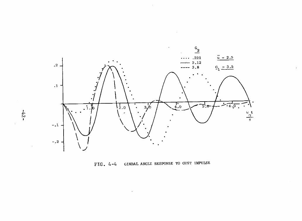
The response of the gyro gimbal angle to a gust impulseis illustrated in Fig. 4-4. For the same set of roots, the
maximum values of a for each value of G2 are approximately
the same. These maximum values, which equal approximately
0.2 for the three cases considered, indicate the possibility
(for large .values of w /b corresponding to large gusts or
small wing chords) thag the small-angle approximation intro-
duced in Appendix B to linearize the equations may become
invalid. For example, GL = 3.5, G2 = 2.12, w /b = 3.0 re-
sults inama x = 33 deg.
To obtain the effect of varying G2 on maximum power re-
quirements, a parametric optimization study was done in which
the root locations corresponding to the smallest absolute
value of maximum power for varying values of G2 and U were
calculated. For each G 2 and u the minimum power values occur-
red for approximately those root locations associated with
minimum gain values. The results are shown in Fig. 4-5.Small values of G? correspond to situation (1) as discussed in
Section 3.4 in which four critical roots exist. The large
values of control torque are needed not only to null the gyro
gimbal, but to provide energy to increase the flutter velocityof the system. For large values of G2, there are only twocritical roots associated with the gyro gimbal angle. The min-imum value of the power parameter, P, for a particular u occurs
,at the transition between two and four critical roots. Thismini um corresponds to the actual minimum power required if
IGz a remains constant as G2 is varied.
To obtain an actual estimate of power required, the
-40-
G 2.1 -
.221- 2.12
S... 3.8
.05 . * * u = 2.5, * G = 3.5
T 0 I I _tc - 4 3 0 44 51
-.05
-. 1
FIG. 4-2 TORQUE RESPONSE TO GUST IMPULSE
.0 - G 2
... .221
S---- 2.12S *---- 3.8
.5 u = 2.5
G = 3.5. * • . -1
(1 2 0. 2 .0\ 5 0 \ .0 6 .0
-. 5 - .
-1.0
FIG. 4-3 POWER RESPONSE TO GUST IMPULSE
-41-
G 2
..... 221 u = 2.5
2 .12
.2 / ---- 3.8 G = 3.5
.1 1 ".0 3/ 4.0 '5-. o
Og I
•t e wt
-.2
FIG. 4-4 GIMBAL ANGLE RESPONSE TO GUST IMPULSE
following set of values was selected, compatible with the
chosen values of G1 and G2:
TABLE 4-2
G2 = 3.8
H = 6.0 kg-m2w sec
IGz = 0.09 kg-m2
wa = 10 Hz
b = 1.5 ft.
The corresponding maximum value of power is 0.007 HP.
Also shown in Fig. 4-5 are the values of power associatedwith two of the reduced feedback cases discussed in Sec. 3-4,and identified on the figure. These values indicate that by pro-
per selection of the root locations a reduction in feedbackcomplexity can be made without a significant increase in power
requirements (illustrated by 0). However, since the system ei-
genvalues cannot be arbitrarily determined with reduced feed-
back systems, the noncritical root locations and the stabilitylevel of the controlled system may be sufficiently altered
to produce increased power requirements. The maximum gimbalangles corresponding to the root locations used to determine
Fig. 4-5 are shown in Fig. 4-6. The minimum values of a foreach u occur at the value of G2 corresponding to the minimumvalue of P in Fig. 4-5. These two curves indicate that selectinga value of G2 corresponding to a value of uF equal to the maxi-
mum desired flutter velocity results in the "best" design, withregard to minimizing values of power, while keeping variationsof a to a minimum. This, of course, would be subject to size
constraints on the CMG itself. The large values of o/(wg/b)may be prohibitive for any practical design. These values can
be reduced by relocating the critical and noncritical roots ofthe system with corresponding increases in power requirements.From Eq. 4-20, it can be seen that increases in GI, holding G2constant, can also result in a decrease in a. These would besome of the many tradeoffs to be made in the more detailed designprocedure used when developing an actual system.
-43-
8.0-
G1 = 3.5-1
6.0-
x 4.0- Reduced FeedbackiT = 2.5
S- K5 = .1
2.0- u
K3 = .4 .2.5K5 = .Oi 2.3Kg = .1 1.9
0 1.0 2.0 3.0 4.0 5.0 6.0
FIG. 4-5 MINIMIZED MAXIMUM POWER RESPONSE TO GUST IMPULSE
-44-
.3 u
2.5
2.3
S .2- .9(w /b)
.1 -1
I I I I I I G20.0 1.0 2.0 3.0 4.0 5.0 6.0
FIG. 4-6 MAXIMUM GIMBAL ANGLE CORRESPONDING TO THE MINIMIZEDMAXIMUM POWER RESPONSE
-45-
V. OPEN-LOOP CONTROl. HARACTFRTqTTC SOF A THREE-DIMENSIONAL CANTILEVER WING WITH
CMG CONTROLLER
5.1 CMG Orientation
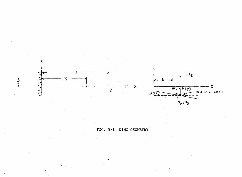
The basic approach to the design analysis of the three
dimensional wing parallels the typical section analysis
developed in Chap. II. The wing geometry is shown in
Fig. 5-1. It is assumed to be an unswept, constant chord,cantilever wing, with rigid chordwise sections, having a
straight elastic axis and uniform structural properties.
Before developing the equations of motion for the wing con-
troller system, the most effective orientation of the CMG
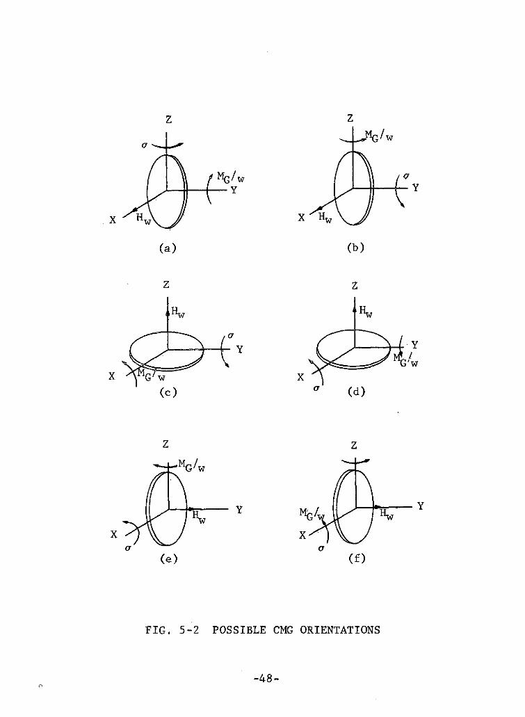
should be determined. As can be seen from Figure 5-2, six
possible orientations exist, depending on the direction of
the gyro's precession and spin axes (for illustrative pur-
poses, only a single rotor of the twin-gyro controller is
shown). To be most effective, the output torque produced
by the CMG on the wing, MG/w, should be directed about an
axis of rotation of the wing (i.e., the X or Y axis).
Thus, cases 5-2b and 5-2e, which provide moments about the
Z-axis, would obviously not be a suitable choice. A pre-
liminary analysis has also shown, for the particular set
of parameters selected in this thesis (see Section 2.2),
that directing the CMG output torque about the X-axis,cases 5-2c and 5-2f, does not provide adequate control
capability. Consequently, cases 5-2a and 5-2d appear to be
the most suitable CMG orientations. For low control torque
levels, the difference between the two orientations can be
considered negligible, and for the following analysis case
5-2a was selected. The equations of motion for the control
moment gyro in this orientation are derived in Appendix B.
5.2 Wing-Controller Equations of Motion
The dynamical equations of motion for the coupled tor-
sion and bending of a cantilever wing are derived in a number
of classic aeroelastic references, including Refs. 20 and 21.
These equations, with the inclusion of the CMG terms from
Appendix B, can be written
mh(y, t)+mGh (yt)8 (y-yG)+EIh 4t)o ~i(y,t)
(5-1)+S Ga(y,t)8(y- y G ) = -LD -L
-46-
z
- L,LDc YG b
• - U= -XY lb h(y)
(y) _/ _ ELASTIC AXIS
Ma,MD
FIG. 5-1 WING GEOMETRY
Z Z
MG/w
MG w IY Y
X H X Hw
(a) (b)
z z
y y
GX w
(c) a (d)
z z
XY
a o(e) (f)
FIG. 5-2 POSSIBLE CMG ORIENTATIONS
-48-
Sa h(y, t)+SaGh (yt)(y-yG)+Iaa (y, t)+IaG (y,t)8(y-YG)
- GJg2 a(y t ) + Hwb(y,t)8(y-yG) = MD + Me (5-2)ay 2
- Hwa(yG,t)+IGz (YG,t) = Tc(YG,t) (5-3)
With the boundary conditions of a cantilever beam:
at y = o, h =2h = a = 0ay (5-4)
at y =, 82 h _ - 3 h a = 0Sy 2 ay 3 ay
The CMG is treated as a concentrated mass and is assumed
to generate a concentrated torque.about the Y-axis. Rota-
tional inertia terms about the X-axis and CMG effects on
flexural and torsional rigidity are considered negligible.
A number of methods are available for developing
solutions to the above equations. Runyan and Watkins (28)
developed a solution for a uniform wing with arbitrarily
placed, concentrated masses by extending the treatment of
Goland (29), in which the differential equations are attacked
directly. To obtain flutter information, this is the most
accurate approach for a uniform wing, but it does not allow
for a suitable means to determine control gains or to deal
with wings having non-uniform properties. A practical methodfor performing flutter calculations is based on the assump-
tion that the motion of the system can be approximated by asuperposition of a finite number of certain selected modal
functions. This type of analysis is often referred to as a
Rayleigh type or the Rayleigh-Ritz method. Since a contin-uous system, such as a wing, possesses infinite degrees offreedom, the accuracy of the results depends, in general, on
the number and choice of modal functions to be used. Thetwo most common choices for these functions are either the
coupled or uncoupled modes of oscillation of the system ina vacuum, since these functions satisfy structural boundaryconditions. In determining the uncoupled modes, bending andtorsion are assumed independent, such that the inertialcoupling terms, those containing Sa, are neglected in the
equations of motion. Physically, this is equivalent to
assuming, for pure bending, for example, that the mass
-49-
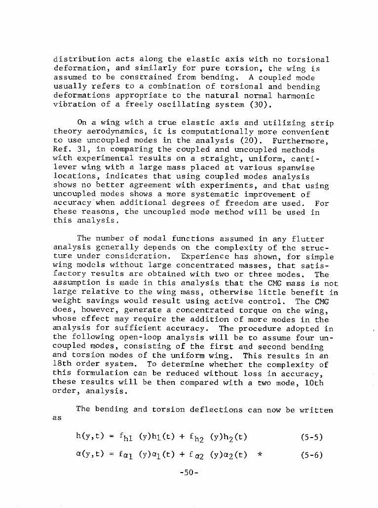
distribution acts along the elastic axis with no torsionaldeformation, and similarly for pure torsion, the wing isassumed to be constrained from bending. A coupled modeusually refers to a combination of torsional and bendingdeformations appropriate to the natural normal harmonicvibration of a freely oscillating system (30).
On a wing with a true elastic axis and utilizing striptheory aerodynamics, it is computationally more convenientto use uncoupled modes in the analysis (20). Furthermore,Ref. 31, in comparing the coupled and uncoupled methodswith experimental results on a straight, uniform, canti-lever wing with a large mass placed at various spanwiselocations, indicates that using coupled modes analysisshows no better agreement with experiments, and that usinguncoupled modes shows a more systematic improvement ofaccuracy when additional degrees of freedom are used. Forthese reasons, the uncoupled mode method will be used inthis analysis.
The number of modal functions assumed in any flutteranalysis generally depends on the complexity of the struc-t1e under consideration. Experience has shown, for simplewing models without large concentrated masses, that satis-factory results are obtained with two or three modes. Theassumption is made in this analysis that the CMG mass is notlarge relative to the wing mass, otherwise little benefit inweight savings would result using active control. The CMGdoes, however, generate a concentrated torque on the wing,whose effect may require the addition of more modes in theanalysis for sufficient accuracy. The procedure adopted inthe following open-loop analysis will be to assume four un-coupled modes, consisting of the first and second bendingand torsion modes of the uniform wing. This results in an18th order system. To determine whether the complexity ofthis formulation can be reduced without loss in accuracy,these results will be then compared with a two mode, 10thorder, analysis.
The bending and torsion deflections can now be writtenas
h(y,t) = fhl (y)hl(t) + fh 2 (y)h2 (t) (5-5)
a(y,t) = fal (y)a l (t) + fa2 (y)a2(t) * (5-6)
-50-
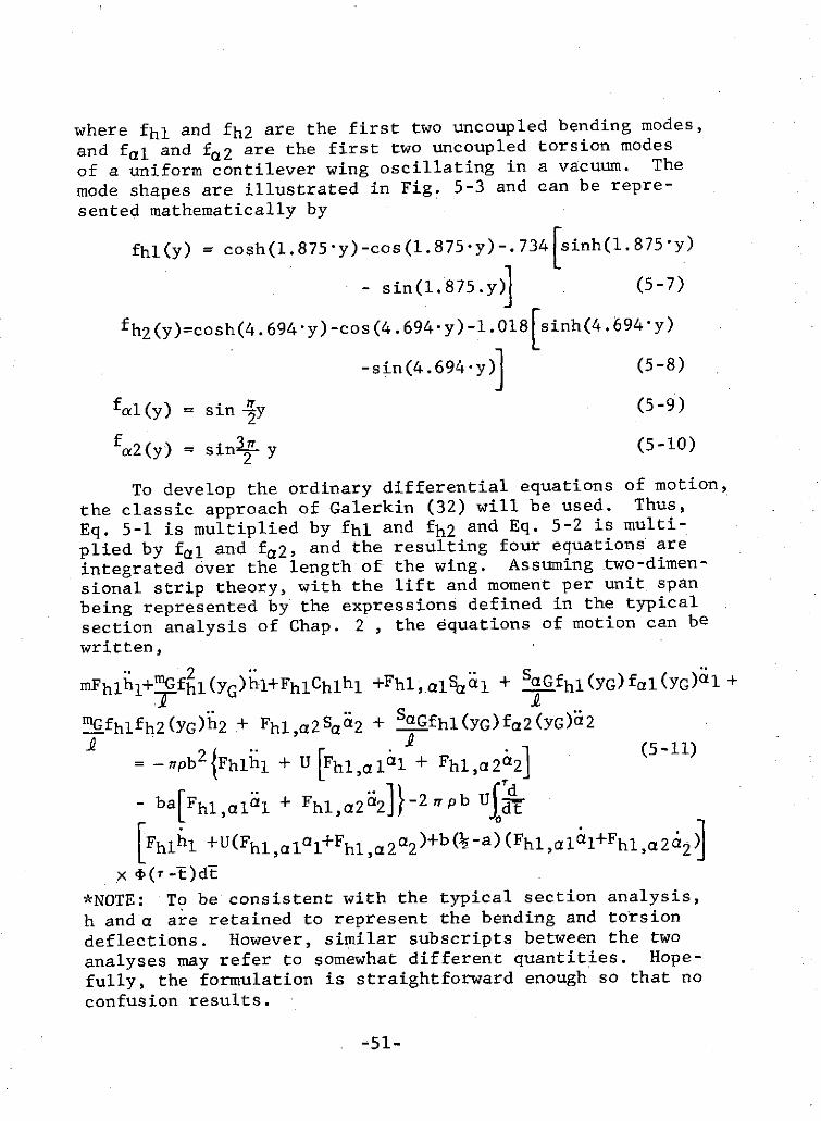
where fhl and fh2 are the first two uncoupled bending modes,and fal and fa2 are the first two uncoupled torsion modes
of a uniform contilever wing oscillating in a vacuum. The
mode shapes are illustrated in Fig. 5-3 and can be repre-
Another often used procedure for obtaining the equa-tions of motion is to first develop expressions for the kineticand potential energies of the system and then apply Lagrange'sequations (33). The resulting equations would, of course,be the same.
5.3 Open-Loop Characteristics of Wing-Controller System
Paralleling the procedure of Chap. 2 to determine thecharacteristic equation, Eqs. 5-11 and 5-12 are divided bynpb 3 , Eqs. 5-13 and 5-14 are divided by rpb 4 , and the Lap-
lace transform of the resulting equations is taken. Theequations become, in matrix form,
-54-
+2i 2 ()}hl 20-
FhlG 2 x~l/-as +1+1-a)p(S) u {(xa2tLa)S2+[+(12aX'g]us hOji .111 0 2 02 hr +2jj2,(;) Fhl.a2 b
2 2 -2
F hlal Fh2,al + a~--k22,~) 9 cl 3 a 0
2 2- - r 2 - 1 r22i+I~
+rc-6 (1+2a)o(i) }F.2
0 0 .- G0 1 i -G0 2s, -S UI
where, in this case
- Uu s=
al
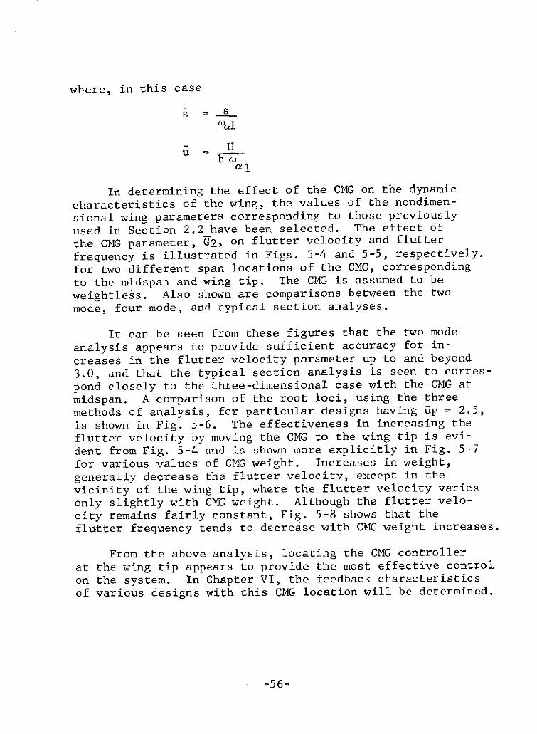
In determining the effect of the CMG on the dynamic
characteristics of the wing, the values of the nondimen-
sional wing parameters corresponding to those previously
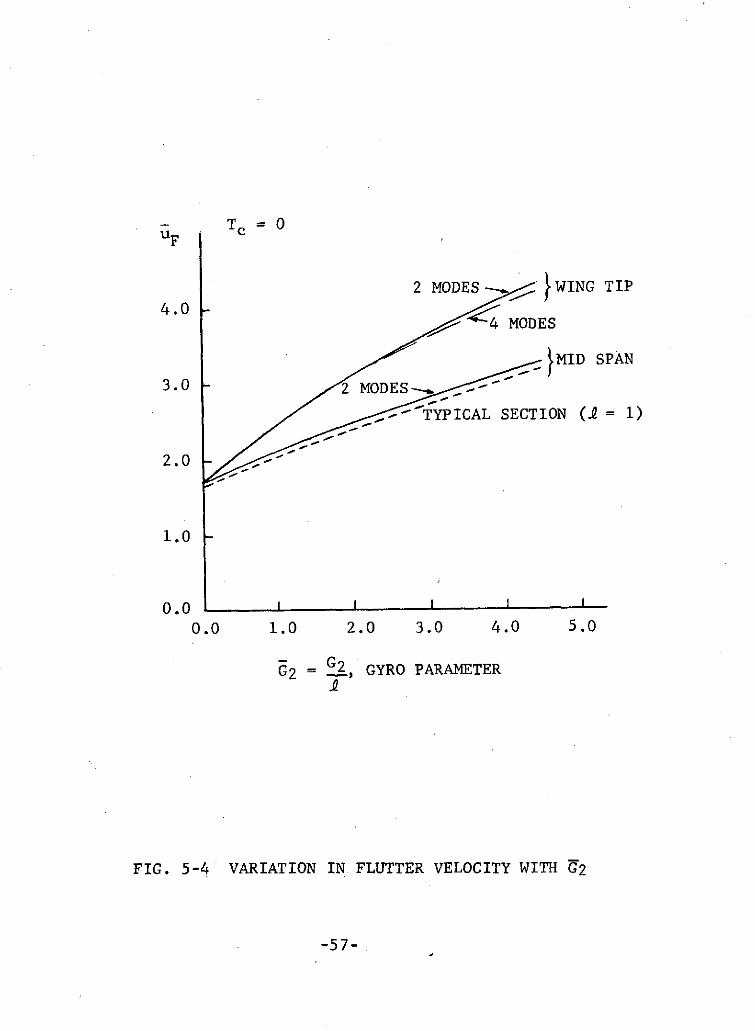
used in Section 2.2 have been selected. The effect of
the CMG parameter, G2, on flutter velocity and flutter
frequency is illustrated in Figs. 5-4 and 5-5, respectively.
for two different span locations of the CMG, corresponding
to the midspan and wing tip. The CMG is assumed to be
weightless. Also shown are comparisons between the two
mode, four mode, and typical section analyses.
It can be seen from these figures that the two mode
analysis appears to provide sufficient accuracy for in-
creases in the flutter velocity parameter up to and beyond
3.0, and that the typical section analysis is seen to corres-
pond closely to the three-dimensional case with the CMG at
midspan. A comparison of the root loci, using the three
methods of analysis, for particular designs having 5F = 2.5,is shown in Fig. 5-6. The effectiveness in increasing the
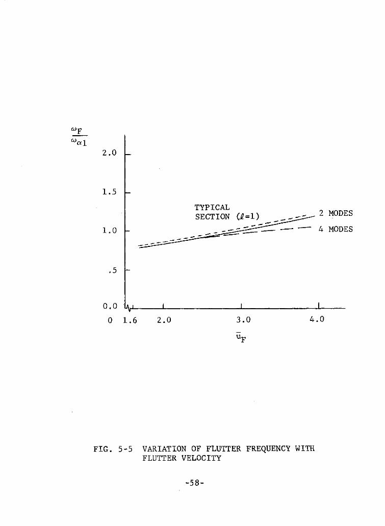
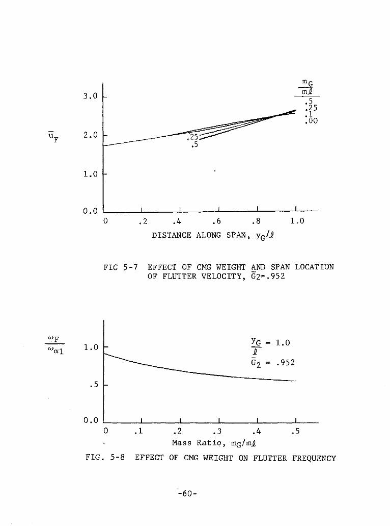
flutter velocity by moving the CMG to the wing tip is evi-
dent from Fig. 5-4 and is shown more explicitly in Fig. 5-7
for various values of CMG weight. Increases in weight,
generally decrease the flutter velocity, except in the
vicinity of the wing tip, where the flutter velocity varies
only slightly with CMG weight. Although the flutter velo-
city remains fairly constant, Fig. 5-8 shows that the
flutter frequency tends to decrease with CMG weight increases.
From the above analysis, locating the CMG controller
at the wing tip appears to provide the most effective control
on the system. In Chapter VI, the feedback characteristics
of various designs with this CMG location will be determined.
-56-
- Tc =0uF
2 MODES WING TIP
4 MODES
) MID SPAN
3.0 - 2 MODES-
-~s-TYPICAL SECTION (a = 1
2.0
1.0
0.0 I0.0 1.0 2.0 3.0 4.0 5.0
G2 = 2, GYRO PARAMETER
FIG. 5-4 VARIATION IN. FLUTTER VELOCITY WITH Z2
-57-
OF
2.0
1.5
TYPICALSECTION (=1) - 2 MO
1.0 4 MODES
.5 -
0.0
0 1.6 2.0 3.0 4.0
uF
FIG. 5-5 VARIATION OF FLUTTER FREQUENCY WITHFLUTTER VELOCITY
-58-
IMAGINARY
u=2.5 4.0
3.0s-Plane
-3.0
u=3.0 2.5
2 MODES
4 MODES
TYPICAL SECTION 2.0
1.0
2.5 3.03.0 2.5
OTHER ROOTS ALONG AXIS
REAL-.8 -.6 -.4 -.2 C .2
FIG. 5-6 ROOT LOCUS COMPARISON OF 3 METHODSOF ANALYSIS, UF = 2.5
-59-
mG
3.0 -.5.25.1.00
UF 2.0 .
1.0
0 .0 I I I I0 .2 .4 .6 .8 1.0
DISTANCE ALONG SPAN, YG/-
FIG 5-7 EFFECT OF CMG WEIGHT AND SPAN LOCATIONOF FLUTTER VELOCITY, G2=.952
OF YG = 1.01.0 -.0
G2 .952
.5
0.0
0 .1 .2 .3 .4 .5
Mass Ratio, mG/ml
FIG. 5-8 EFFECT OF CMG WEIGHT ON FLUTTER FREQUENCY
-60-
VI. FEEDBACK CONTROL OF THE THREE-DIMENSIONALWING-CONTROLLER SYSTEM
6.1 Introduction
Obtaining solutions to the feedback control problemof a continuous, elastic, unstable system, such as a wingin an airstream travelling faster than the critical fluttervelocity, can be most difficult. Exact solutions of just
the aeroelastic problem have been developed for only a few
special cases. Since the wing is actually an infinite-
degree-of-freedom system, and thus has infinite states,
new, more realistic, meanings must also be found for the
concepts of controllability and observability (34). In
Chap. 5, it was shown how the continuous system could be
approximated by an equivalent system with finite degreesof freedom, and furthermore, in our particular case, how.
describing the system with only two modes of vibrationcan result in reasonable accuracy in determining the
system's flutter characteristics. There is no guarantee,however, that this simple model will be valid for the feed-back case. Higher modes may be excited and possibly drivenunstable in attempting to control the lower modes. Thus,certain questions arise in examining the control problemof even the approximate system: 1) What is the minimumnumber of modes to be included in the analysis to insurethat the controlled system is stable over the requiredrange of velocities?, 2) What is the minimum number ofcontrols needed for controllability and/or stability?,3) What are the essential feedback parameters to achievestability?, and 4) How many measurements are needed toestablish observability for the system? These questionswill be discussed in some detail in the following sections.
6.2 State Variable Selection and Controllability
The method of design using arbitrary dynamics and theconcept of controllability were discussed in Chap. 3. Forconvenience in determining the control characteristics ofthe three-dimensional system, the system equations, Eqs.5-17, are first put in standard state variable form. Asin the typical section case, a decision as to which quan-tities are selected as states must be made, with the addedcomplexity for the three-dimensional wing in deciding howmany vibrational modes to assume in the analysis. Eachadditional assumed mode increases the number of states byfour, due to the particular modeling of the incompressible
-61-
aerodynamics. Thus, for the two mode Lnalysis, the system
could be represented by ten states (two states corresponding
to the CMG), and eighteen states would be needed if four
modes were included in the analysis. It is obvious that
the amount of analysis and various design requirements such
as sensor and feedback selection, could be substantially
reduced if only two modes are necessary to obtain accurate
control information. For that reason, and because the two
mode analysis proved adequate in determining the open-loop
system characteristics, a feedback control design using two
modes was first attempted. The gains obtained from this
analysis were then used to determine the characteristics
of the system, approximated by four modes, to verify the
accuracy of the two mode method.
The selection of the ten states defining the two mode
system is made consistent with those chosen in the typical
Following the procedure developed in Section 3.1, the
appropriate portions of the set of Eqs. 5-17 are multiplied
by D,(§) and the inverse Laplace transform taken, remem-
bering that in the two mode case
fh2 = fa2 =, Fh2 = F2 Fh2,al Fh2, 2 -
Fa2,hl = Fa2,h2 = 0
The resulting equations are then written using the state
variable definitions, Eqs. 6-1 to 6-10, and put in the
matrix form, Fig. 6-1, where the matrix elements are
defined in Appendix D.
As discussed in Section 3.3, a necessary and suffi-
cient condition for modal controllability is that the con-
trollability matrix be nonsingular. It can be shown that
this matrix defined by
C = [G FG . . ......... iFn-1G
is non-singular for the parameters selected in this analysis
with G11, G01 >0 , u 0.. Furthermore, the system remains
controllable, using just one controller, even when the num-
ber of modes in the analysis is increased, so long as the
quantities, fhi(YG) and fa(YG) do not equal zero. This
requirement is met with the CMG at the wing tip. These
results are, of course, theoretical, with the assumed modes
and aerodynamic model being approximations. Experimental
verification of controllability of any design would be
necessary to insure that the control or sensors are not
located at the node of a particular mode of vibration.
6.3 Design by Arbitrary Dynamics
To investigate the feedback characteristics of thesystem defined in Eqs. 6-11, a particular CMG-controller,having a G2-value of 1.13 and CMG-to-wing mass and momentof inertia ratios of .05, was selected for analysis. Forflutter velocity increases up to 50% (i.e., uF = 2.55),this system will have only two critical roots. Based on
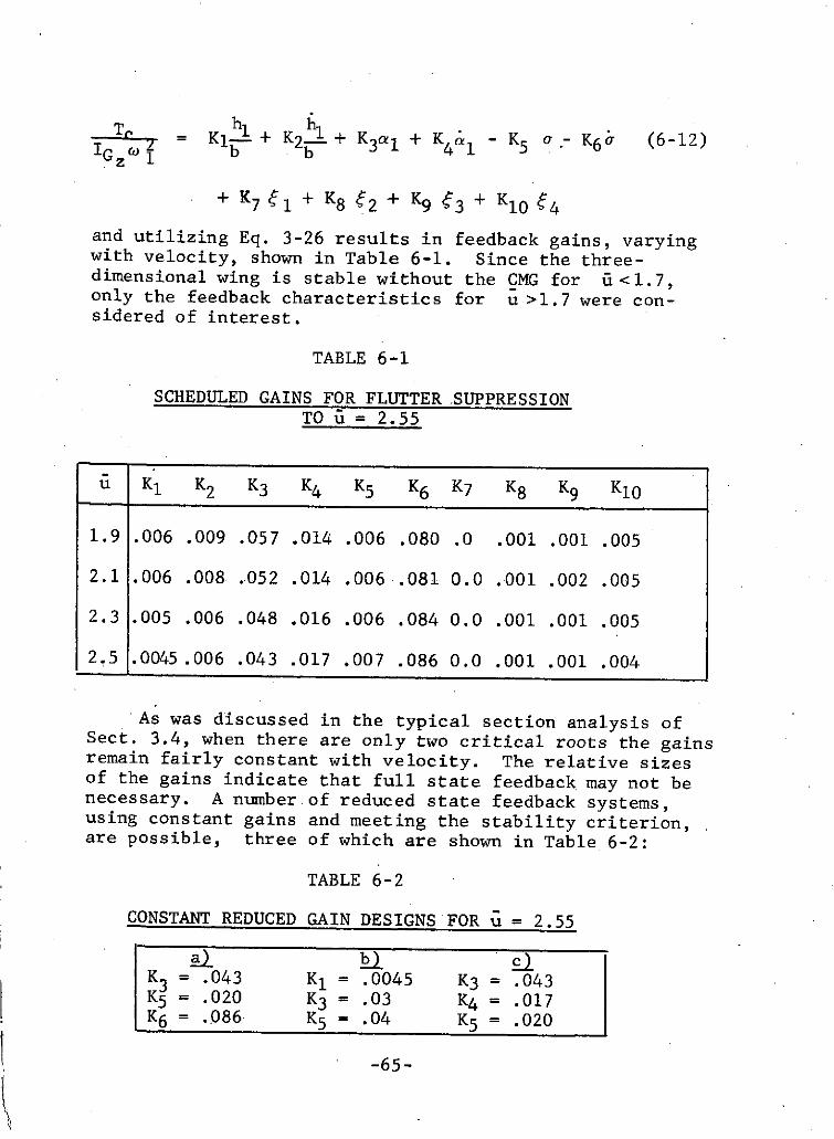
the typical section analysis in Sect. 4.3, this systemwill be the design having minimum power requirements, ifthe critical roots are placed on the real axis. Assuminga control law of the form
and utilizing Eq. 3-26 results in feedback gains, varyingwith velocity, shown in Table 6-1. Since the three-dimensional wing is stable without the CMG for ii<1.7,only the feedback characteristics for u >1.7 were con-sidered of interest.
TABLE 6-1
SCHEDULED GAINS FOR FLUTTER ,SUPPRESSIONTO u = 2.55
As was discussed in the typical section analysis ofSect. 3.4, when there are only two critical roots the gainsremain fairly constant with velocity. The relative sizesof the gains indicate that full state feedback may not benecessary. A number.of reduced state feedback systems,using constant gains and meeting the stability criterion,are possible, three of which are shown in Table 6-2:
A comparison of the root loci obtained for the sche-duled gains of Table 6-1 and the constant reduced gains ofTable 6-2, case a), which requires the feedback of a, a ,and &, is shown in Fig. 6-2. The final selection of anyfeedback scheme will depend on sensor and power requirements,with any variation from the gains in Table 6-1 resulting inincreased power.
The simplest control design would be to just feedbacka . However, the large power increase associated with
this design (cf. Fig. 4-5) would probably make it infeasible.
6.4 Higher Mode Instability
Although a number of designs have been developed forsuppressing flutter in the system defined by Eqs. 6-11,there is no assurance, as yet, that the gains determinedwill stabilize this system with higher modes included inthe analysis. An example of the occurrence of such ahigher order instability is presented in Ref. 35 for aflexible launch vehicle. To guard against such occurrencesin a design, usually more modes are included in the controlanalysis than are necessary to accurately determine thepassive flutter characteristics. For example, in Ref. 36,although three modes were sufficient to predict the criticalflutter velocity, seven modes were used in the controlsystem design analysis.
To determine the effect on higher modes of the designsdeveloped in the previous section, constant gains, corres-ponding to u = 2.5 in Table 6-1, were used, and the secondbending and second torsion modes were included in describingthe wing-controller system. The resulting root locus isshown in Fig. 6-3. From the figure, the problem of higherorder instability appears not to exist. Similar results arefound for the gains in Table 6-2. This is not the case,however, if different root locations are selected for thecritical roots. Figure 6-4 shows the locations of rootscorresponding to different values of the imaginary part ofthe critical root at a velocity corresponding to u = 2.5.From Fig. 6-3, it can be seen that, although the rootsassociated with the first bending and torsion branches re-main relatively constant as the imaginary value of thecritical root is increased, the higher order roots do vary,
-66-
IMAGINARY
s-Plane
SCHEDULED GAINS 2.0
CONSTANT REDUCED GAINS
G2 = 1.13
U =1.0
1.9 u
U=3.0 2.5 1.0
--------.- -- 2 5
2.5OTHER ROOTS ALONG AXIS 3.0 -4
REAL-.6 -.4 -.2
FIG. 6-2 COMPARISON BETWEEN SCHEDULED GAINSAND REDUCED CONSTANT GAINS
-67-
IMAGINARY
s-Plane
-4.0 G2 = 1.13u = 2.5
3.0
-3.0
u = 3.0 2.5 1.9 1.0
2.0
3.0 2.53.0 2.52.5 -1.03.0
OTHER ROOTS ALONG AXIS
-.6 -.4 -.2 REAL
Fig. 6-3 FOUR MODE ROOT LOCUS USING OPTIMIZED CONSTANTGAINS FROM TWO MODE ANALYSIS
-68-
IMAGINARY
INCREASING
u = 2.55.0 IMAGINARY VALUE
G2 = 1.13 OF CRITICAL ROOT
s-Plane
-3.0
00
-2.0
O 4 MODE ONLY
O1 2 & 4 MODE
S1. x NO CONTROL
OTHER ROOTS CRITICALALONG AXIS ROOTS -- I
-. 6 -. 4 -. 2 0 .2 .4REAL
FIG. 6-4 COMPARISON OF FOUR MODE ROOTS USING TWO MODEGAINS FOR DIFFERENT LOCATIONS OF CRITICAL ROOTS
-69-
with one root eventually becoming and staying unstable.Similar results will occur, if other prescribed rootlocations in the two mode analysis cause the gain values,and thus the power requirements to be large. The gainsin Table 6-1 were selected by minimizing the value of powerrequired for control upon encountering an impulsive gustdisturbance. This criterion caused the minimum perturba-tion in the non-critical roots and resulted in low gainvalues. If other optimum criteria are established, forexample, by defining certain weighting matrices in thequadratic synthesis analysis discussed in Sect. 4-1, pro-blems in higher mode instability may occur.
6.5 System Observability
As was discussed in Section 3.5, the sensor problemcould be reduced if all the states could be estimatedfrom a measurement of a . The system, Eqs. 6-11, will beobservable if the observability matrix, defined in Eq. 3-27,is non-singular. It can be shown that the observabilitymatrix is non-singular for the parameters selected in thisanalysis for G0 1 , G11 , >0, ii0. The system does not re-main observable with a single measurement, however, ifhigher modes are included in the analysis, even if fhi(YG)and fai(YG) do not equal zero. The relationship betweenthe modes (cf.Eqs. 5-5 & 5-6) requires additional measure-ments as the number of selected modes increases, since onlya(t) (or h(t)) and not al(t) and a2 (t) can be determinedfrom a single measurement. This illustrates another advan-tage to the design of Sect. 6-3, which required but twomodes for a suitable design.
-70-
VII. CONCLUSIONS & RECOMMENDATIONS
7.1 Conclusions
An analysis, utilizing modern control techniques for
designing active flutter suppression systems with a con-
trol moment gyro as the controller, has been presented.
The following conclusions can be drawn:
1. The concepts of modern control theory provide a
well-organized, systematic, and mathematically
powerful approach to the design of active flutter
suppression systems. Using the method of arbi-
trary dynamics, feedback gains, which produce
stable systems having satisfactory response
characteristics, can be easily obtained in a
straightforward manner over a wide range of
structural, geometric, and aerodynamic parameters.
The solution for optimal gains based on a variety
of cost functionals can be incorporated into the
design not only for the single input/single output
case considered here, but can be adapted to multi-
input/multi-output systems. If full state feed-
back systems are not feasible, these methods
provide starting points in obtaining reduced feed-
back and suboptimal designs.
2. The control moment gyro has certain attractive
design features which warrant its consideration
as an alternative to aerodynamic surfaces for ac-
tively suppressing flutter modes. Controller
designs characterized by simplicity, quick re-
sponse, and low power requirements can be developed.
3. Although the flutter suppression analysis in this
thesis was accomplished using a control moment gyro,certain design results can be applied generally to
any controller.
(a) Controllability can be achieved using only
one, properly placed, controller for signifi-
cant increases in flutter velocity.
(b) When using arbitrary dynamics, noncritical
roots should remain constant.
-71-
(c) For introductory analyses, relative feed-back gain size is a reasonable design
criterion for evaluating prospective designs.
(d) Optimization criterion, such as minimizing aquadratic cost function, should be usedcautiously, with the possibility of higherorder instability kept in mind.
(e) Two-dimensional analysis can provide valuableinsight in developing practical design pro-
cedures and determining basic system charac-teristics.
(f) Certain aerodynamic surface parameters, suchas flap width and/or length, can play a role
similar to G2 in selecting optimum designs.
7.2 Recommendations
In the field of active flutter suppression there are
many possible areas of further research, many of which arediscussed in Ref. 4. Recommendations evolving more directly
from the results of this thesis are the following, some of
which are presently being pursued at Stanford:
1. Application of the control moment gyro concept asprimary control device or in conjunction withaerodynamic surfaces, to an actual wing model, todetermine realistic sizing and power requirements.
2. Application of the design techniques, procedures,and tradeoff studies outlined in this thesis toan aerodynamic surface control, to compare power,performance, and complexity of design.
3. Establishment of a practical design optimizationcriterion, thereby providing a more thoroughunderstanding into the cause and prevention ofhigher order instability.
4. Development of suitable mathematical modeling of
the aerodynamics in subsonic, transonic, and super-
sonic flow over complex elastic structures to allowthe broad application of modern control technikes.
-72-
5. Establishment of sensor and estimator require-ments to determine the required feedbacks forstable and optimum designs.
-73-
APPENDIX A
AERODYNAMIC FORCES ON A TWO-DIMENSIONAL
WING SECTION IN UNSTEADY INCOMPRESSIBLE FLOW
Critical to the application of certain design techni-
ques used in this thesis, such as the root-locus diagram and
state variable formulation, is the particular modeling of
the two-dimensional, transient aerodynamic forces using the
Wagner indicial function. Although this concept is familiar
to most aeroelasticians, it is felt that a brief description
of its derivation is warranted.
First, the aerodynamic forces in two-dimensional, in-
compressible flow on a surface oscillating in simple harmonic
motion are considered. Using potential flow theory, Theodorsen
(22) obtained results for lift and moment in which the solu-
tion was separated into two components, corresponding to
circulatory and non-circulatory portions of the flow field.
The resulting equations can be written
L = pb2[h+Ua-bag+2tpUbC(k) [h-Ua+b( -a)a] (A-l)
M= rpb2[ba-Ub ( -a)-b 2 ( +a82 )
+2pUb 2 (a+)C (k) h+Ua+b ( -a)] (A-2)
The non-circulatory components are contained in the
first set of terms in Eqs. A-I and A-2, and are also valid
for arbitrary motion as long as it is small. In the second
set of terms, C(k) is,commonly known as the Theodorsen
function and is evaluated by solving certain complex inte-
grals resulting from the potential flow formulation. The
Theodorsen function is complex and can be written after
integration H1(2)(k)
C(k) = F(k) + iG(k) = Hl(2)(k)+ iHo(")(k) (A-3)
-74-
where HI(2) and Ho(2) are Hankel functions of the second
kind. A complex polar plot of C(k) is shown below.
G(k).5 1.0
0 K= K0 F(k)K=0
-.1 K=1.0 K=.05
-. 2 K=.4 K=.1K=.2
-.3
Fig. A-1 COMPLEX POLAR PLOT OF C(k)
These results have been used extensively for flutter
prediction for many years, and can still provide a source
of relatively reliable reference data for large aspect ratio
wings even though they actually have supersonic flutter
speeds (20).
Theodorsen's formulation for C(k) is invalid, however,for convergent oscillations in arbitrary motion. One
method for solving this problem employs a superposition
(Duhamel) integral of the linear results for simple harmonic
motion.
Corresponding to the steady state case, Wagner (23)
determined the lift on an airfoil considering the growth of
circulation about the airfoil as it starts impulsively from
rest to a uniform velocity, U. The form of this lift is
L = 2 7pb Uw t (E)
where w is the downwash velocity, E is a non-dimensional
time, and C (t) is the Wagner indicial function. Wagner's
-75-
function was originally calculated by using a vortex-sheetmethod (23). The method described here somewhat parallelsthe approach in Ref. 24.
Because of linearity, it is possible to determine thelift due to circulation for any arbitrary motion of the air-foil by superposition. In an interval dE the downwash w(t)increases by the amount, dw(E) dE. When dt is small, this
dE
may be regarded as an impulsive increment and the lift canbe determined by convolution:
L = 2b w(o) V(o) (t-t') dt (A-4)
It is a convenient fact that in incompressible flowthe circulatory component of force on an airfoil is deter-mined by the downwash velocity at the 3/4-chord (cf Eqs.A-I & A-2) which has the form
w3/4c = h +U + b ( 2-a) (A-5)
Thus, only one Wagner function is required to describe thearbitrary motion. The Wagner function is evaluated byassuming
ikew(t) = woe
in Eq. A-4 and comparing the results to Theodorsen's form forthe oscillatory lift, Eq. A-I, which can be written
L = 2 b pUC(k)w oeikt (A-6)
After some manipulation of terms, the Wagner function can bewritten as
s(t) = sin kE dk (A-7)
and its behavior as a function of t is illustrated in Fig.A-2.
-76-
.5
0 5 10 15 20 t
FIG A-2 WAGNER INDICIAL LIFT FUNCTION
Although 94(t) has a relatively simply graphical form, it
is not mathematically expressible in terms of well-known
functions. Therefore, several accurate approximations have
been developed (20). For convenience in taking Laplace
transforms, a particularly useful one for application in
this thesis, is the form
() 1- .165e-.0 4 55 - .335e - .3 t (A-8)
-77-
Appendix B
GYRO EQUATIONS OF MOTION
In the twin-gyro controller, the equal but oppositeprecession of the gyro rotors can be obtained by using twotorquing motors or by using one motor with proper gearingbetween the two gyros. The development of the CMG contri-bution to the typical-section equations of motion followsthe derivation in Ref. 19, in which one motor is used.For this analysis, the following assumptions are made:
(1) The CMG twin-gyro controller is rigidlyattached to the wing.
(2) The spin speed of each rotor is assumed equaland constant with respect to its respectivegimbals.
(3) The rotor spin axes are principal axes.
(4) The moment of inertia of the typical section-controller combination about the elastic axis(y) is independent of the gyro gimbal anglea (Fig. B-1).
(5) The typical section rotates only about theelastic axis.
Z
z
g2 a
Y,y
X h g
T
FIG. B-1 TWIN-GYRO CONTROLLER ROTORS
-78-
The total angular momentum of the gyro controller is
HTG = HGl + HG2 + HF (B-l)
where
HTG = total angular momentum of the twin-gyrocontroller
HGI = total angular momentum of gyro 1, includingrotor and gimbal
HG2 = total angular momentum of gyro 2
HF = total angular momentum of twin-gyrocontroller "fixed" elements.
From Fig. B-1
GI g cos x + (hg sino + Ily&)y(B-2)
+ Ilzoz
where
hg1 = angular momentum of gyro rotor 1
Ily = moment of inertia of gyro 1 about y axis
Ilz = moment of inertia of gyro 1 about z axis.
Similarly,
HG 2 = -hg2 coso x + (hg2 sin + 12y&)y - 12z&Z; (B-3)
also
HF = IFay (B-4)
where IF is the moment of inertia of the fixed componentsabout the y axis. Combining Eqs. B-l, B-2, B-3, and B-4and letting hgl = hg2 , Ilz = I2z yield
HTG = (Hw sin a + ly&) y (B-5)
-79-
where
Hw = 2hgl = 2hg2
Iy = Ily + I2y + IF
Equation B-5 illustrates the features of the twin-gyrocontroller in which the momentum change will occur about the
y axis and crosscoupling terms cancel.
To obtain the contribution of the controller to the
typical-section equations of motion, Eq. B-5 is differentiatedwith respect to time in an inertial reference frame and ex-
pressed in the wing reference frame by the theorem of Coriolisas
i w
HTG TG TG w/G. (B-6)
Here the superscript i indicates differentiation with re-spect to time in an inertial frame; the superscript windicates time differentiation in the wing frame; Z7 isthe angular velocity of the wing frame with respect to theinertial frame which is this analysis equals &9 ; and Mw/Gis the reaction moment of the wing on the controller.
Equation B-6 can be written in scalar notation since
the momentum and rotation are about the y axis. It becomes
iHTG = y + H acos = Mw/G . (B-7)
An equation involving the control torque and the gyro
parameters can be obtained by differentiating Eqs. B-2 and
B-3 and applying the theorem of Coriolis. This results in
i (Ilz&+hgl o sina) +(hgl a cosa +ly&)yHG1
+ (Ilza-hgl acosa )z = T (B-8)
-80-
-- = (-I2z&+hg2 sin a )+(hg2 icosa +12y&HG2
+ (-I2zU+hg2 acosa )z = T , (B-9)
where T and T2 are the torques on gyro 1 and 2 respec-tively.
Subtracting Eq. B-9 from Eq. B-8 and taking the, compo-
nent in the Z direction gives
IGz H - H a cosa = TI z - T2z (B-10)
where
IGz = lz + 1 2z
Tlz = torques about z axis on gyros 1 and 2
T2z respectively.
Since the gyros are geared together,
Tlz = -T2z'
Therefore, let
Tlz - T2 z = 2Tlz = Tc
where Tc is defined as the control torque supplied by the
torque motor on the twin-gyro system about the z axis.
Equation B-10 becomes
IGz i - Hw . cos o = Tc. (B-11)
With the assumption of small gimbal-angle oscillations about
a = 0, Eqs. B-7 and B-11 can be linearlized by setting
cosa;l. The linearized equations are
I + Hwa = W/G (B-12)
-H + IGzo = Tc. (B-13)
-81-
Equations B-12 and B-13 are now used in conjunction with theequations of motion for the typical section to describe themotion of the wing-controller system and are applicable foruse in the three-dimensional case under the assumptions ofChap. 5.
-82-
APPENDIX C
TYPICAL SECTION OPEN-LOOP CHARACTERISTIC EQUATION
The characteristic equation described in Chapter II is
1. Johannes, R. P., "Performance Advantages Offered by
Advanced Flight Control Technology", AIAA Paper No.
70-874, July 1970.
2. Johannes, R. P., "Active Flutter Control-Flight Test
System Synthesis", JACC Paper No. 7-El, August 1971.
3. Swaim, R. L., "Aircraft Elastic Mode Control", Journal
of Aircraft, Vol. I, No. 2, February 1971, pp. 65-71.
4. Thompson, G. 0. and Kass, G. J., "Active Flutter
Suppression -- An Emerging.Technology", Journal of
Aircraft, Vol. 9, No. 3, March 1972, pp. 230-235.
5. Topp, L. J., "Potential Performance Gains by Use of a
Flutter Suppression System", JACC Paper No. 7-B3,August 1971.
6. Thiesen, J. G., and W. C. Robinette, "Servo Control
of Flutter", AIAA Structural Dynamics and Aeroelastic
Specialist Conference Proceedings, April 1969, pp.
228-240.
7. Moon, F. C., and Dowell, E. H., "The Control of Flutter
Instability in a Continuous Elastic System using
Feedback", AIAA/ASME llth Structures, Structural
Dynamics, and Materials Conference, Volume of Techni-
cal Papers on Structural Dynamics, Denver, April
1970.
8. Kalmbach, C. F., "Feedback Control of Flutter Instabi-
lity in a Continuous Elastic System", AIAA Journal,
Vol. 10, No. 5, May 1972, pp. 711-712.
9. Hodges, G. E., "Active Flutter Suppression - B-52
Controls Configured Vehicle", AIAA Paper No. 73-322,1973.
10. Triplett, W. E., Kappus, H. F., and Landy, R. J.,"Active Flutter Control: An Adaptable Application
to Wing/Store Flutter", AIAA Paper No. 73-194, 1973.
11. Nissim, E., "Flutter Suppression Using Active Controls
Based on the Concept of Aerodynamic Energy", NASA
TN D-6199, March 1971.
-89-
12. Miller, B., "USAF Plans Advanced Fighter Program",Aviation Week & Space Technology, July 16, 1973,pp. 14-16.
13. White, J. S. and Hansen, Q. M., "Study of a SatelliteAttitude Control System Using Integrating Gyros as
Torque Sources", NASA TN D-1073, September 1961.
14. Cannon, R. H., Jr., "Basic Response Relations forSatellite Attitude Control Using Gyros", Proceedingsof IFAC, Butterworths, London, 1963, pp. 535-544.
15. Havill, J. R. and Ratcliff, J. W., "A Twin-Gyro Atti-
tude Control System for Space Vehicles", NASA TN
D-2419, August 1964.
16. Liska, D. J. and Jacot, A. D., "Control Moment Gyrosin Attitude Control", Journal of Spacecraft and
Rockets, Vol. 3, No. 9, September 1966, pp. 1313-
1320.
17. Huston, R. L., "Twin-Gyro Attitude Control Systems",Journal of Spacecraft and Rockets, Vol. 3, No. 7,July 1966, pp. 1136-1138.
18. Campbell, R. A., "Performance of a Twin-Gyro AttitudeControl System Including Passive Compensation and aNonlinear Control Law", NASA TN D-5868, August 1970.
19. Pasternack, S., Jr., "Attitude Control of HoppingVehicles", Ph.D. Dissertation, May 1971, Dept. ofAeronautics and Astronautics, Stanford University,Stanford, Calif.
20. Bisplinghoff, R. L., Ashley, H., and Halfman, R. L.,Aeroelasticity, Addison-Wesley, Cambridge, Mass., 1955.
21. Bisplinghoff, R. L. and Ashley, H., Principles ofAeroelasticity, John Wiley, New York, 1962.
22. Theodorsen, T., "General Theory of Aerodynamic In-stability and the Mechanism of Flutter", NACAReport 496, April 1935.
-90-
23. Wagner, H., "Uber Die Entstehung Des DynamischenAuftriebes von Tragflugeln," Z. Angew. Math. Mech.,Bd5, Heft 1, Feb. 1925.
24. Garrick, I. E., "On Some Reciprocal Relations in theTheory of Nonstationary Flows", NACA TR 629, 1938.
25. Gopinath, B., "On the Identification and Control ofLinear Systems", Ph.D. Dissertation, 1968, Dept.of Electrical Engineering, Stanford University,Stanford, Ca.
26. Bryson, A. E., Jr., and Y.-C. Ho, Applied OptimalControl, Blaisdell, Waltham, Mass., 1969.
27. Hall, W. E., Jr., and Bryson, A. E., Jr., "OptimalControl and Filter Synthesis by Eigenvector Decom-position", SUDAAR No. 436, November 1971, Dept. ofAeronautics and Astronautics, Stanford University,Stanford, Calif.
28. Runyan, H. L., and Watkins, C. E., "Flutter of aUniform Wing with an Arbitrarily Placed Mass Accordingto a Differential-Equation Analysis and a Comparisonwith Experiment", NACA TN 1848, 1949.
29. Goland, M., "The Flutter of a Uniform Cantilever Wing",Journal of Applied Mechanics, Vol. 12, No. 4, Dec.1945, pp. 197-208.
30. Woolston, D. S. and Runyan, H. L., "Appraisal of Methodof Flutter Analysis Based on Chosen Modes of Compari-son with Experiment for Cases of Large Mass Coupling",NACA TN 1902, 1949.
31. Woolston, D. S. and Runyan, H. L., "On the Use ofCoupled Modal Functions in Flutter Analysis", NACATN 2375, 1951.
32. Fung, Y. C., An Introduction to the Theory of Aero-elasticity, Dover, New York, 1969.
33. Scanlan, R. H. and Rosenbaum, R., Introduction to theStudy of Aircraft Vibration and Flutter, Dover,New York, 1968.
-91-
34. Wang, P. K., "Control of Distributed Parameter Systems",Advances in Control Systems, Vol. 1, Chap. 3, pp.
75-172, Academic Press, N. Y., 1964.
35. Rynaski, E., Whitbeck, R., and Dolbin, B., Jr.,"Sensitivity Considerations in the Optimal Control
of a Flexible Launch Vehicle", CAL Report No.
BE-2311-Fl, Cornell Aeronautical Laboratory, Inc.,Buffalo, N. Y., June 1967.
36. Triplett, W. E., "A Feasibility Study of Active Wing/
Store Flutter Control", JACC Paper No. 7B4, August