Modern Physics Blackbody radiation Experience show that the temperature of a hot and a cold object placed close to each other equalize in vacuum as well. All macroscopic objects in all temperature emit (and absorb) thermal radiation spontaneously. This radiation consists of electromagnetic waves. The energy of the electromagnetic waves emitted by a surface, in unit time and in unit area, depends on the nature of the surface and on its temperature. The thermal radiation emitted by many ordinary objects can be approximated as blackbody radiation. A perfectly insulated cavity that is in thermal equilibrium internally contains black- body radiation and will emit it through a hole made in its wall, provided the hole is small enough to have negligible effect upon the equilibrium. The (absolute) blackbody absorbs all energy, and reflects nothing, which is of course an idealization. A black-body at room temperature appears black, as most of the energy it radiates is infra-red and cannot be perceived by the human eye. Black-body radiation has a characteristic, continuous frequency spectrum that depends only on the body's temperature. The spectrum is peaked at a characteristic frequency that shifts to higher frequencies (shorter wavelengths) with increasing temperature, and at room temperature most of the emission is in the infrared region of the electromagnetic spectrum. Wien’s displacement law indicates that the maximum of the energy distribution is displaced within the radiation spectrum of a blackbody in case of a change in temperature. max T b λ = where b is called Wien's displacement constant, is equal to 2.89×10 −3 Km.
Transcript
Modern Physics
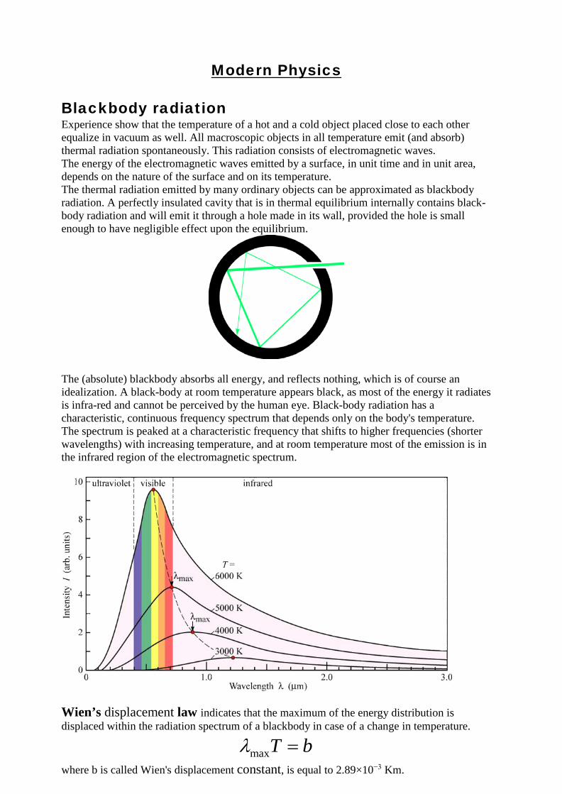
Blackbody radiation Experience show that the temperature of a hot and a cold object placed close to each other equalize in vacuum as well. All macroscopic objects in all temperature emit (and absorb) thermal radiation spontaneously. This radiation consists of electromagnetic waves. The energy of the electromagnetic waves emitted by a surface, in unit time and in unit area, depends on the nature of the surface and on its temperature. The thermal radiation emitted by many ordinary objects can be approximated as blackbody radiation. A perfectly insulated cavity that is in thermal equilibrium internally contains black-body radiation and will emit it through a hole made in its wall, provided the hole is small enough to have negligible effect upon the equilibrium.
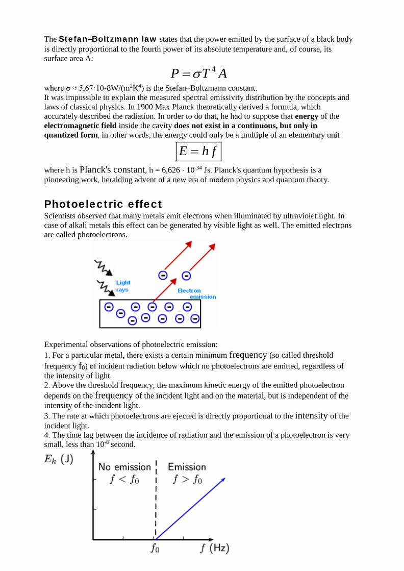
The (absolute) blackbody absorbs all energy, and reflects nothing, which is of course an idealization. A black-body at room temperature appears black, as most of the energy it radiates is infra-red and cannot be perceived by the human eye. Black-body radiation has a characteristic, continuous frequency spectrum that depends only on the body's temperature. The spectrum is peaked at a characteristic frequency that shifts to higher frequencies (shorter wavelengths) with increasing temperature, and at room temperature most of the emission is in the infrared region of the electromagnetic spectrum.
Wien’s displacement law indicates that the maximum of the energy distribution is displaced within the radiation spectrum of a blackbody in case of a change in temperature.
maxT bλ = where b is called Wien's displacement constant, is equal to 2.89×10⁻³ Km.
The Stefan–Boltzmann law states that the power emitted by the surface of a black body is directly proportional to the fourth power of its absolute temperature and, of course, its surface area A:
4P T Aσ= where σ ≈ 5,67·10-8W/(m2K4) is the Stefan–Boltzmann constant. It was impossible to explain the measured spectral emissivity distribution by the concepts and laws of classical physics. In 1900 Max Planck theoretically derived a formula, which accurately described the radiation. In order to do that, he had to suppose that energy of the electromagnetic field inside the cavity does not exist in a continuous, but only in quantized form, in other words, the energy could only be a multiple of an elementary unit
E h f= where h is Planck's constant, h = 6,626 ⋅ 10-34 Js. Planck's quantum hypothesis is a pioneering work, heralding advent of a new era of modern physics and quantum theory.
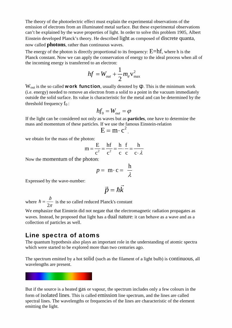
Photoelectric effect Scientists observed that many metals emit electrons when illuminated by ultraviolet light. In case of alkali metals this effect can be generated by visible light as well. The emitted electrons are called photoelectrons.
Experimental observations of photoelectric emission: 1. For a particular metal, there exists a certain minimum frequency (so called threshold frequency f0) of incident radiation below which no photoelectrons are emitted, regardless of the intensity of light. 2. Above the threshold frequency, the maximum kinetic energy of the emitted photoelectron depends on the frequency of the incident light and on the material, but is independent of the intensity of the incident light. 3. The rate at which photoelectrons are ejected is directly proportional to the intensity of the incident light. 4. The time lag between the incidence of radiation and the emission of a photoelectron is very small, less than 10-8 second.
The theory of the photoelectric effect must explain the experimental observations of the emission of electrons from an illuminated metal surface. But these experimental observations can’t be explained by the wave properties of light. In order to solve this problem 1905, Albert Einstein developed Planck’s theory. He described light as composed of discrete quanta, now called photons, rather than continuous waves. The energy of the photon is directly proportional to its frequency: E=hf, where h is the Planck constant. Now we can apply the conservation of energy to the ideal process when all of the incoming energy is transferred to an electron:
2max
1 v2out ehf W m= +
Wout is the so called work function, usually denoted by φ. This is the minimum work (i.e. energy) needed to remove an electron from a solid to a point in the vacuum immediately outside the solid surface. Its value is characteristic for the metal and can be determined by the threshold frequency f0 :
0 outhf W ϕ= = If the light can be considered not only as waves but as particles, one have to determine the mass and momentum of these particles. If we use the famous Einstein-relation
2E m c= ⋅ , we obtain for the mass of the photon:
2 2
E hf h f hmc c c c c λ
= = = ⋅ =⋅
Now the momentum of the photon: h m c pλ
= ⋅ =
Expressed by the wave-number:
kp =
where π2h
= is the so called reduced Planck's constant
We emphasize that Einstein did not negate that the electromagnetic radiation propagates as waves. Instead, he proposed that light has a dual nature: it can behave as a wave and as a collection of particles as well.
Line spectra of atoms The quantum hypothesis also plays an important role in the understanding of atomic spectra which were started to be explored more than two centuries ago. The spectrum emitted by a hot solid (such as the filament of a light bulb) is continuous, all wavelengths are present.
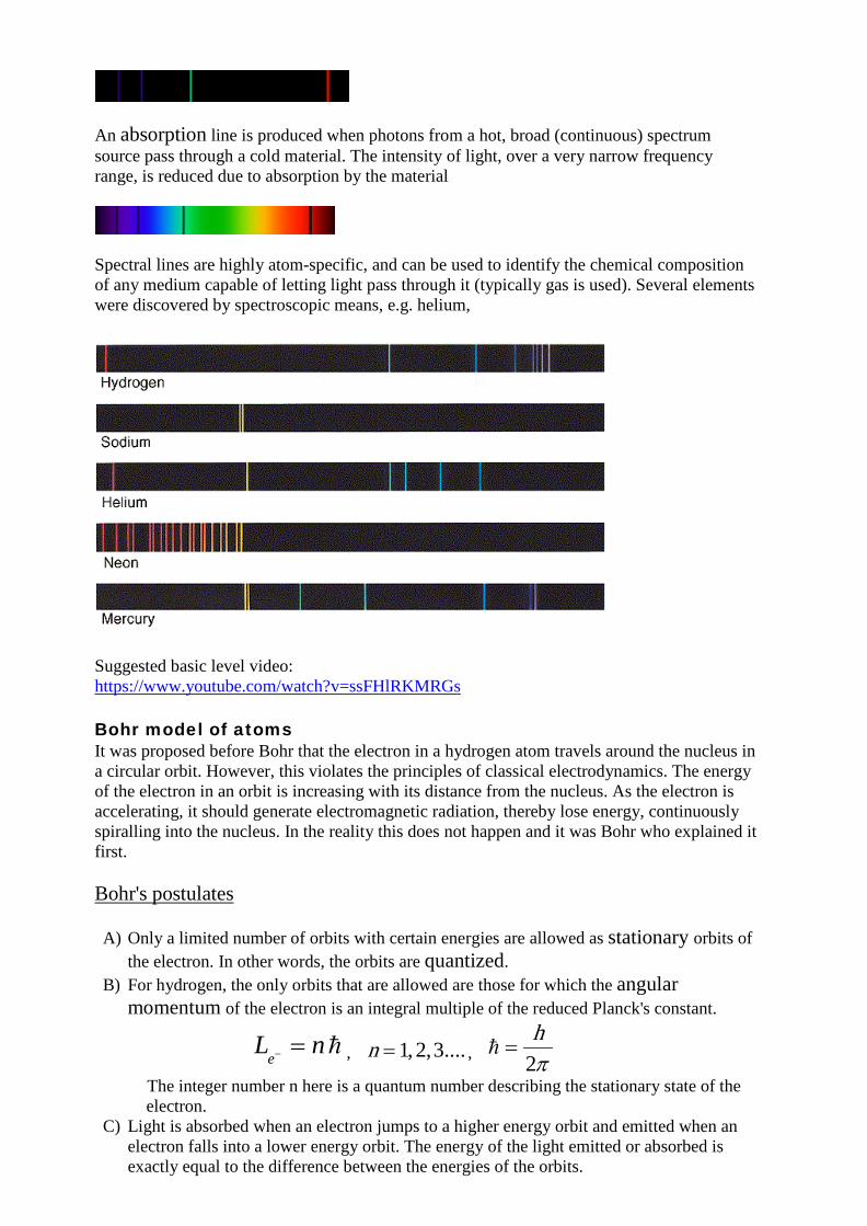
But if the source is a heated gas or vapour, the spectrum includes only a few colours in the form of isolated lines. This is called emission line spectrum, and the lines are called spectral lines. The wavelengths or frequencies of the lines are characteristic of the element emitting the light.
An absorption line is produced when photons from a hot, broad (continuous) spectrum source pass through a cold material. The intensity of light, over a very narrow frequency range, is reduced due to absorption by the material
Spectral lines are highly atom-specific, and can be used to identify the chemical composition of any medium capable of letting light pass through it (typically gas is used). Several elements were discovered by spectroscopic means, e.g. helium,
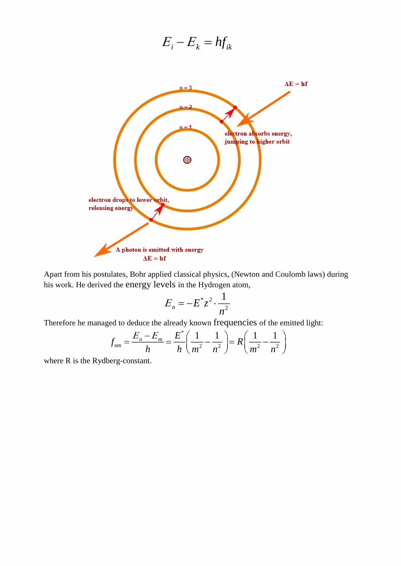
Suggested basic level video: https://www.youtube.com/watch?v=ssFHlRKMRGs Bohr model of atoms It was proposed before Bohr that the electron in a hydrogen atom travels around the nucleus in a circular orbit. However, this violates the principles of classical electrodynamics. The energy of the electron in an orbit is increasing with its distance from the nucleus. As the electron is accelerating, it should generate electromagnetic radiation, thereby lose energy, continuously spiralling into the nucleus. In the reality this does not happen and it was Bohr who explained it first. Bohr's postulates A) Only a limited number of orbits with certain energies are allowed as stationary orbits of
the electron. In other words, the orbits are quantized. B) For hydrogen, the only orbits that are allowed are those for which the angular
momentum of the electron is an integral multiple of the reduced Planck's constant.
eL n− = , ....3,2,1=n , π2
h=
The integer number n here is a quantum number describing the stationary state of the electron.
C) Light is absorbed when an electron jumps to a higher energy orbit and emitted when an electron falls into a lower energy orbit. The energy of the light emitted or absorbed is exactly equal to the difference between the energies of the orbits.
Apart from his postulates, Bohr applied classical physics, (Newton and Coulomb laws) during his work. He derived the energy levels in the Hydrogen atom,
* 22
1= − ⋅n E z
nΕ
Therefore he managed to deduce the already known frequencies of the emitted light: *
2 2 2 2
1 1 1 1− = = − = −
n mnm
Ef Rh h m n m n
Ε Ε
where R is the Rydberg-constant.
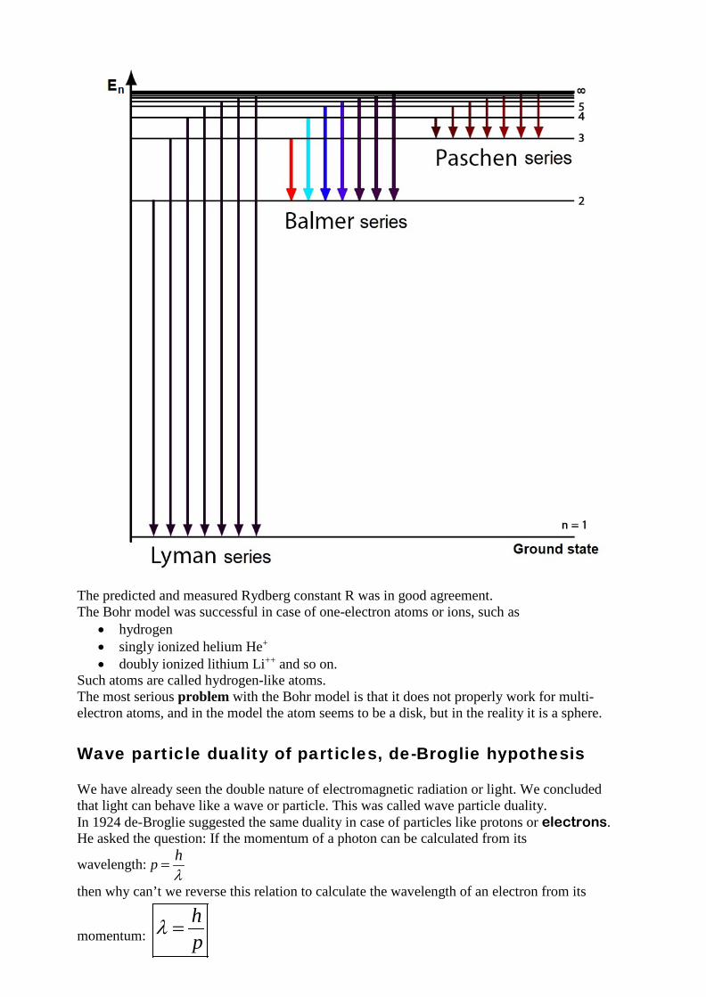
The predicted and measured Rydberg constant R was in good agreement. The Bohr model was successful in case of one-electron atoms or ions, such as
• hydrogen • singly ionized helium He+ • doubly ionized lithium Li++ and so on.
Such atoms are called hydrogen-like atoms. The most serious problem with the Bohr model is that it does not properly work for multi-electron atoms, and in the model the atom seems to be a disk, but in the reality it is a sphere. Wave particle duality of particles, de-Broglie hypothesis We have already seen the double nature of electromagnetic radiation or light. We concluded that light can behave like a wave or particle. This was called wave particle duality. In 1924 de-Broglie suggested the same duality in case of particles like protons or electrons. He asked the question: If the momentum of a photon can be calculated from its
wavelength: p hλ
=
then why can’t we reverse this relation to calculate the wavelength of an electron from its
momentum: hp
λ =
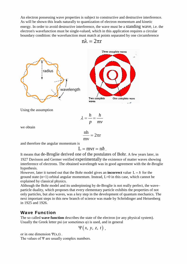
An electron possessing wave properties is subject to constructive and destructive interference. As will be shown this leads naturally to quantization of electron momentum and kinetic energy. In order to avoid destructive interference, the wave must be a standing wave, i.e. the electron's wavefunction must be single-valued, which in this application requires a circular boundary condition: the wavefunction must match at points separated by one circumference
n 2 rλ = π
Using the assumption
h hp mv
λ = =
we obtain nh 2 rmv
= π
and therefore the angular momentum is L mvr n= = .
It means that de-Broglie derived one of the postulates of Bohr. A few years later, in 1927 Davisson and Germer verified experimentally the existence of matter waves showing interference of electrons. The obtained wavelength was in good agreement with the de-Broglie hypothesis. However, later it turned out that the Bohr model gives an incorrect value L = for the ground state (n=1) orbital angular momentum. Instead, L=0 in this case, which cannot be explained by classical physics. Although the Bohr model and its underpinning by de-Broglie is not really perfect, the wave–particle duality, which proposes that every elementary particle exhibits the properties of not only particles, but also waves, was a key step in the development of quantum mechanics. The next important steps in this new branch of science was made by Schrödinger and Heisenberg in 1925 and 1926. Wave Function The so called wave function describes the state of the electron (or any physical system). Usually the Greek letter psi (or sometimes φ) is used, and in general
( ), , , x y z tΨ , or in one dimension Ψ(x,t) . The values of Ψ are usually complex numbers.
Only continuous, bounded functions can describe a real physical system, and usually there is
a requirement that the square-integral of Ψ should be bounded: 2
fullspace
dV CΨ <∫
What is the physical meaning of the wave function Ψ for a particle? The wave function describes the distribution of the particle in space. It is related to the probability of finding the particle in various regions. If we imagine a volume element dV around a point, the probability that the particle can be found in that volume element is measured by
2 dVΨ . The so called probability density is 2ρ ∗= Ψ ≡ Ψ Ψ .
The probability of finding a particle in an arbitrary volume is the integral of the probability density:
2(V) 1V V
p dV dVρ= = Ψ <∫ ∫
One can have the information only about where the particle is likely to be, not where it is for sure. Principle of superposition: If ψ1 and ψ2 are possible wave-functions of the system, then the
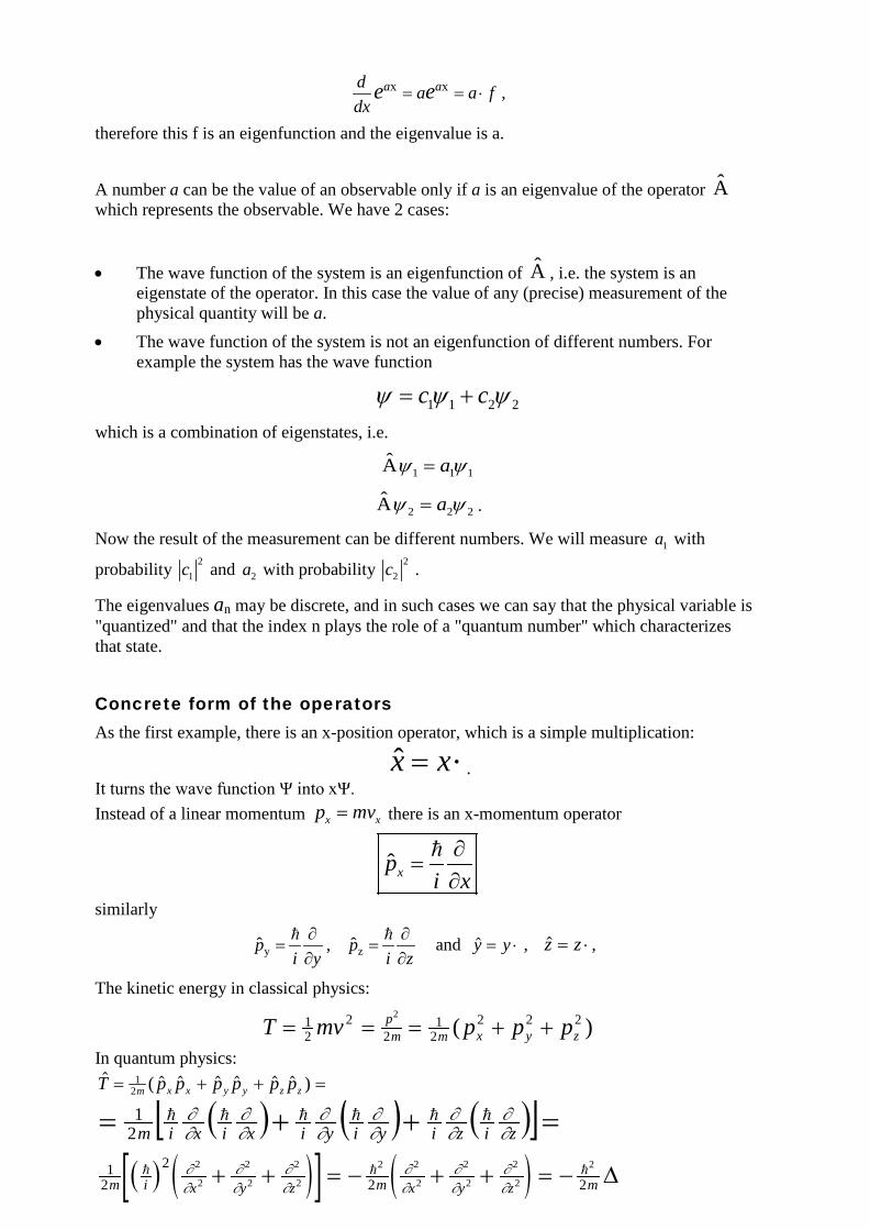
1 1 2 2c cψ ψ ψ= + linear combination is also a possible wave-function. We note that in quantum computing, a qubit or quantum bit is a unit of quantum information—the quantum analogue of the classical binary bit. A qubit is a two-state quantum-mechanical system. In a classical system, a bit would have to be in one state or the other. However, quantum mechanics allows the qubit to be in a superposition of both states at the same time, a property that is fundamental to quantum computing. Operators The observables, i.e. those physical quantities which are dynamical variables (i.e. not constants like m or q) are represented by linear operators, denoted by “hat” on the top of the letter: O . To obtain specific values for physical quantities, for example energy or momentum, you operate on the wavefunction with the quantum mechanical operator associated with that quantity. In linear algebra, an eigenvector of a square matrix is a vector that points in a direction which is invariant under the associated linear transformation (eigen here is the German word meaning self or own). In other words, if v is a nonzero vector, then it is an eigenvector of a square matrix A if Av is a scalar multiple of v . Similarly in case of functions, f is an eigenfunction of an operator A if the action of that operator is only a multiplication of that function by a number:
Af af=
where a is a real or complex number. For example, ddx
is a linear operator and if
xf( ) ax e= then
x xa ad a a fdx
e e= = ⋅ ,
therefore this f is an eigenfunction and the eigenvalue is a.
A number a can be the value of an observable only if a is an eigenvalue of the operator A which represents the observable. We have 2 cases:
• The wave function of the system is an eigenfunction of A , i.e. the system is an eigenstate of the operator. In this case the value of any (precise) measurement of the physical quantity will be a.
• The wave function of the system is not an eigenfunction of different numbers. For example the system has the wave function
1 1 2 2c cψ ψ ψ= +
which is a combination of eigenstates, i.e.
1 1 1A aψ ψ=
2 2 2A aψ ψ= .
Now the result of the measurement can be different numbers. We will measure 1a with
probability 21c and 2a with probability 2
2c .
The eigenvalues an may be discrete, and in such cases we can say that the physical variable is "quantized" and that the index n plays the role of a "quantum number" which characterizes that state.
Concrete form of the operators As the first example, there is an x-position operator, which is a simple multiplication:
x x= ⋅ . It turns the wave function Ψ into xΨ. Instead of a linear momentum x xp mv= there is an x-momentum operator
ˆ xpi x∂
=∂
similarly
y zˆ ˆ,p pi y i z∂ ∂
= =∂ ∂
and y y= ⋅ , z z= ⋅ ,
The kinetic energy in classical physics:
T mv p p ppm m x y z= = = + +1
22
21
22 2 22
( ) In quantum physics: ( )T p p p p p pm x x y y z z= + + =1
2
( ) ( ) ( )[ ]=++= ziziyiyixixim ∂∂
∂∂
∂∂
∂∂
∂∂
∂∂
21
( ) ( )[ ] ( )12
22 2
2
2
2
2
2
2
2 2
2
2
2
2
2
2
m i x y z m x y z m ∂
∂∂∂
∂∂
∂∂
∂∂
∂∂
+ + = − + + = − ∆
T m= −
2
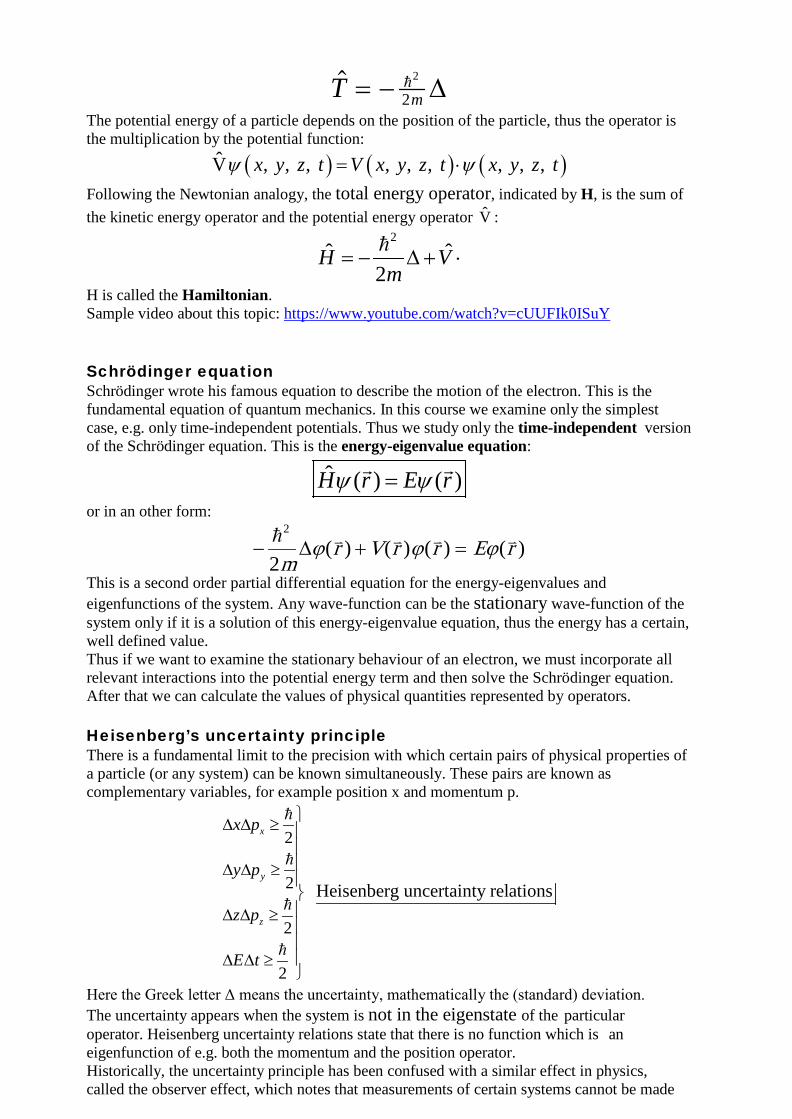
2 ∆ The potential energy of a particle depends on the position of the particle, thus the operator is the multiplication by the potential function:
( ) ( ) ( )V , , , , , , , , , x y z t x y zV t x y z tψ ψ= ⋅ Following the Newtonian analogy, the total energy operator, indicated by H, is the sum of the kinetic energy operator and the potential energy operator V :
2ˆ ˆ
2H V
m= − ∆ + ⋅
H is called the Hamiltonian. Sample video about this topic: https://www.youtube.com/watch?v=cUUFIk0ISuY Schrödinger equation Schrödinger wrote his famous equation to describe the motion of the electron. This is the fundamental equation of quantum mechanics. In this course we examine only the simplest case, e.g. only time-independent potentials. Thus we study only the time-independent version of the Schrödinger equation. This is the energy-eigenvalue equation:
ˆ ( ) ( )H r E rψ ψ=
or in an other form:
− + =
2
2mr V r r E r∆ϕ ϕ ϕ( ) ( ) ( ) ( )
This is a second order partial differential equation for the energy-eigenvalues and eigenfunctions of the system. Any wave-function can be the stationary wave-function of the system only if it is a solution of this energy-eigenvalue equation, thus the energy has a certain, well defined value. Thus if we want to examine the stationary behaviour of an electron, we must incorporate all relevant interactions into the potential energy term and then solve the Schrödinger equation. After that we can calculate the values of physical quantities represented by operators. Heisenberg’s uncertainty principle There is a fundamental limit to the precision with which certain pairs of physical properties of a particle (or any system) can be known simultaneously. These pairs are known as complementary variables, for example position x and momentum p.
2
2
2
2
Heisenberg uncertainty relations
x
y
z
x p
y p
z p
E t
∆ ∆ ≥ ∆ ∆ ≥ ∆ ∆ ≥∆ ∆ ≥
Here the Greek letter Δ means the uncertainty, mathematically the (standard) deviation. The uncertainty appears when the system is not in the eigenstate of the particular operator. Heisenberg uncertainty relations state that there is no function which is an eigenfunction of e.g. both the momentum and the position operator. Historically, the uncertainty principle has been confused with a similar effect in physics, called the observer effect, which notes that measurements of certain systems cannot be made
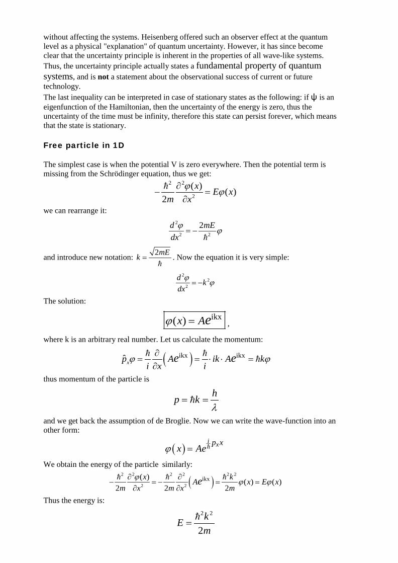
without affecting the systems. Heisenberg offered such an observer effect at the quantum level as a physical "explanation" of quantum uncertainty. However, it has since become clear that the uncertainty principle is inherent in the properties of all wave-like systems. Thus, the uncertainty principle actually states a fundamental property of quantum systems, and is not a statement about the observational success of current or future technology. The last inequality can be interpreted in case of stationary states as the following: if ψ is an eigenfunction of the Hamiltonian, then the uncertainty of the energy is zero, thus the uncertainty of the time must be infinity, therefore this state can persist forever, which means that the state is stationary. Free particle in 1D The simplest case is when the potential V is zero everywhere. Then the potential term is missing from the Schrödinger equation, thus we get:
2 2
2
( ) ( )2
x E xm x
ϕ ϕ∂− =
∂
we can rearrange it: 2
2 2
2d mEdxϕ ϕ= −
and introduce new notation: 2mEk =
. Now the equation it is very simple:
22
2
d kdxϕ ϕ= −
The solution:
ikx( )x Aeϕ = ,
where k is an arbitrary real number. Let us calculate the momentum:
( )ikx ikxˆ xp A ik A ki x i
e eϕ ϕ∂= = ⋅ ⋅ =
∂
thus momentum of the particle is
hp kλ
= =
and we get back the assumption of de Broglie. Now we can write the wave-function into an other form:
( )i xp x
x Aeϕ =
We obtain the energy of the particle similarly:
( )2 2 2 2 2 2
2 2ikx( ) ( ) ( )
2 2 2x kA x E x
m x m x meϕ ϕ ϕ∂ ∂
− = − = =∂ ∂
Thus the energy is: 2 2
2kEm
=
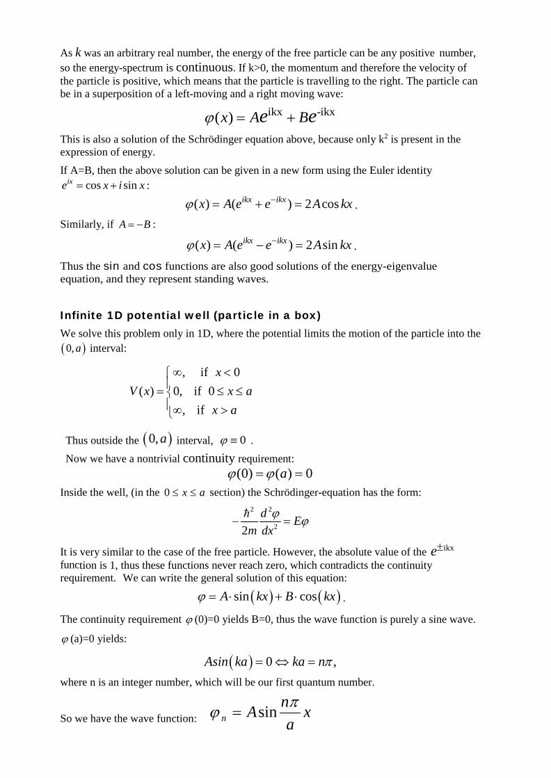
As k was an arbitrary real number, the energy of the free particle can be any positive number, so the energy-spectrum is continuous. If k>0, the momentum and therefore the velocity of the particle is positive, which means that the particle is travelling to the right. The particle can be in a superposition of a left-moving and a right moving wave:
ikx -ikx( )x A Be eϕ = +
This is also a solution of the Schrödinger equation above, because only k2 is present in the expression of energy. If A=B, then the above solution can be given in a new form using the Euler identity
cos sinixe x i x= + :
( ) ( ) 2 cosikx ikxx A e e A kxϕ −= + = .
Similarly, if A B= − :
( ) ( ) 2 sinikx ikxx A e e A kxϕ −= − = .
Thus the sin and cos functions are also good solutions of the energy-eigenvalue equation, and they represent standing waves.
Infinite 1D potential well (particle in a box) We solve this problem only in 1D, where the potential limits the motion of the particle into the ( )0, a interval:
, if 0( ) 0, if 0
, if
xV x x a
x a
∞ <= ≤ ≤∞ >
Thus outside the ( )0,a interval, 0ϕ ≡ . Now we have a nontrivial continuity requirement:
(0) ( ) 0aϕ ϕ= = Inside the well, (in the 0 ≤ ≤x a section) the Schrödinger-equation has the form:
2 2
22d E
m dxϕ ϕ− =
It is very similar to the case of the free particle. However, the absolute value of the ikxe± function is 1, thus these functions never reach zero, which contradicts the continuity requirement. We can write the general solution of this equation:
( ) ( )sin cosA kx B kxϕ = ⋅ + ⋅ .
The continuity requirement ϕ (0)=0 yields B=0, thus the wave function is purely a sine wave.
ϕ (a)=0 yields:
( ) 0 ,Asin ka ka nπ= ⇔ =
where n is an integer number, which will be our first quantum number.
So we have the wave function: ϕπ
n A na
x= sin
Physically this means a standing wave for each n>0. In order to obtain the possible energy
values we substitute back the expression 2mEk =
, and obtain:
2mE a nπ=
.
After rearrangement
24
2 2 2 2 2 22
2mEa n n h= =π π
π
One can see that the energy is quantized and proportional to the square of the n quantum number:
E hma
n=2
22
8
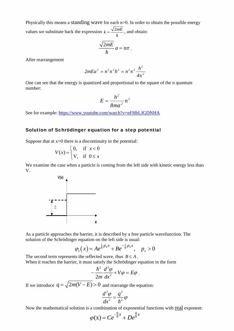
See for example: https://www.youtube.com/watch?v=nFHhLJGDNHA Solution of Schrödinger equation for a step potential Suppose that at x=0 there is a discontinuity in the potential:
0, if 0
( )V, if 0
xV x
x<
= ≤
We examine the case when a particle is coming from the left side with kinetic energy less than V.
As a particle approaches the barrier, it is described by a free particle wavefunction. The solution of the Schrödinger equation on the left side is usual:
( )1 , 0x
i ix xp x p xx Ae Be pϕ −= + >
The second term represents the reflected wave, thus B A≤ . When it reaches the barrier, it must satisfy the Schrödinger equation in the form
2 2
22d V E
m dxϕ ϕ ϕ− + =
.
If we introduce 2 ( ) 0q m V E= − > and rearrange the equation: 2 2
2 2
d qdxϕ ϕ=
Now the mathematical solution is a combination of exponential functions with real exponent:
, ifq xe x→∞ →∞ , which is nonphysical. Thus D=0 and the solution is an
exponentially decreasing real function:
( )2
q xx Ceϕ
−=
The probability density 8 ( )2
2* *( ) ( ) ( )m V Eq x x
x x x C C e C eρ φ φ− −−
= ⋅ = ⋅ ⋅ = ⋅
According to classical physics, a particle of energy E less than the height V of a barrier could not penetrate - the region inside the barrier is classically forbidden. But the wavefunction associated with a free particle must be continuous at the barrier and will show an exponential decay inside the barrier. The penetration depth is the distance inside the potential-step where the probability decreases by a factor e:
0p1(x ) (x )eρ ρ−=
Now the penetration depth is inversely proportional to the square root of the mass and the missing energy:
8 ( )x p m V E
=−
,
and with this notation:
2( ) p
xxx C eρ
−
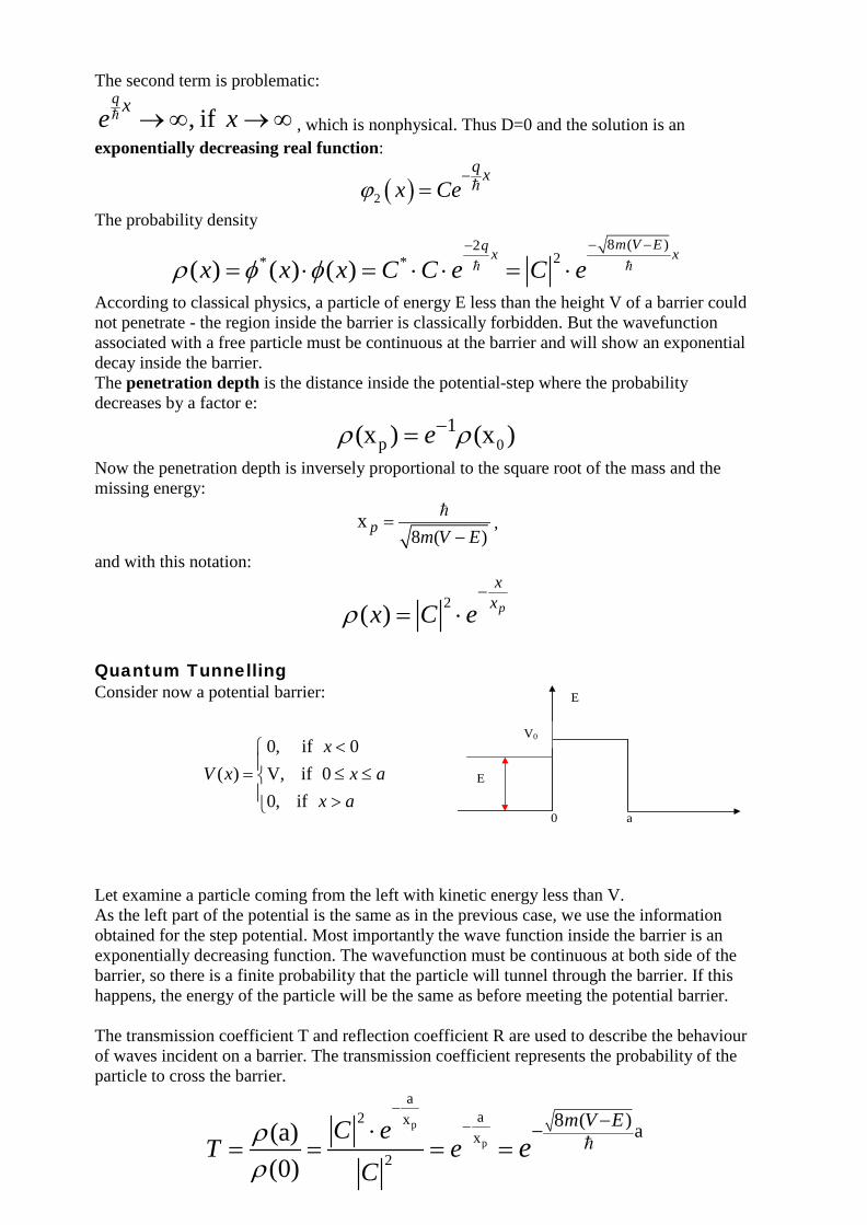
= ⋅ Quantum Tunnelling Consider now a potential barrier:
0, if 0( ) V, if 0
0, if
xV x x a
x a
<= ≤ ≤ >
Let examine a particle coming from the left with kinetic energy less than V. As the left part of the potential is the same as in the previous case, we use the information obtained for the step potential. Most importantly the wave function inside the barrier is an exponentially decreasing function. The wavefunction must be continuous at both side of the barrier, so there is a finite probability that the particle will tunnel through the barrier. If this happens, the energy of the particle will be the same as before meeting the potential barrier. The transmission coefficient T and reflection coefficient R are used to describe the behaviour of waves incident on a barrier. The transmission coefficient represents the probability of the particle to cross the barrier.
p
p
aa2 x
x2
8 ( ) a(a)(0)
m V EC eT e
Ceρ
ρ
−− −⋅
= = = =
0 a
E
V0
E
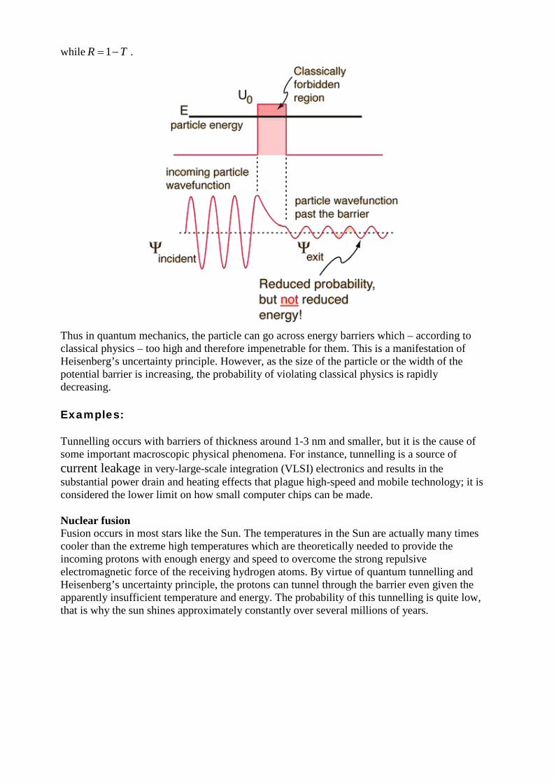
while 1R T= − .
Thus in quantum mechanics, the particle can go across energy barriers which – according to classical physics – too high and therefore impenetrable for them. This is a manifestation of Heisenberg’s uncertainty principle. However, as the size of the particle or the width of the potential barrier is increasing, the probability of violating classical physics is rapidly decreasing. Examples: Tunnelling occurs with barriers of thickness around 1-3 nm and smaller, but it is the cause of some important macroscopic physical phenomena. For instance, tunnelling is a source of current leakage in very-large-scale integration (VLSI) electronics and results in the substantial power drain and heating effects that plague high-speed and mobile technology; it is considered the lower limit on how small computer chips can be made. Nuclear fusion Fusion occurs in most stars like the Sun. The temperatures in the Sun are actually many times cooler than the extreme high temperatures which are theoretically needed to provide the incoming protons with enough energy and speed to overcome the strong repulsive electromagnetic force of the receiving hydrogen atoms. By virtue of quantum tunnelling and Heisenberg’s uncertainty principle, the protons can tunnel through the barrier even given the apparently insufficient temperature and energy. The probability of this tunnelling is quite low, that is why the sun shines approximately constantly over several millions of years.
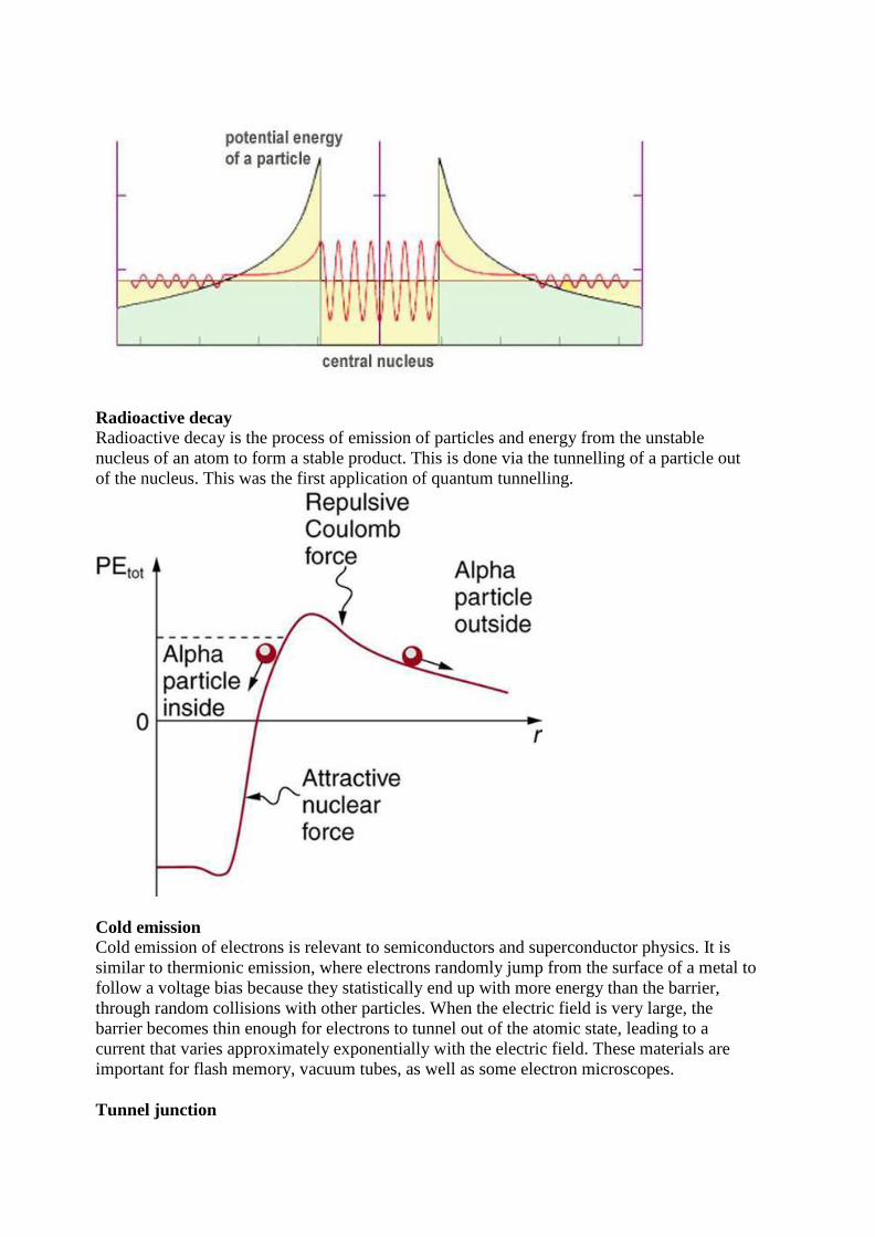
Radioactive decay Radioactive decay is the process of emission of particles and energy from the unstable nucleus of an atom to form a stable product. This is done via the tunnelling of a particle out of the nucleus. This was the first application of quantum tunnelling.
Cold emission Cold emission of electrons is relevant to semiconductors and superconductor physics. It is similar to thermionic emission, where electrons randomly jump from the surface of a metal to follow a voltage bias because they statistically end up with more energy than the barrier, through random collisions with other particles. When the electric field is very large, the barrier becomes thin enough for electrons to tunnel out of the atomic state, leading to a current that varies approximately exponentially with the electric field. These materials are important for flash memory, vacuum tubes, as well as some electron microscopes. Tunnel junction
A simple barrier can be created by separating two conductors with a very thin insulator. These are tunnel junctions, the study of which requires quantum tunnelling. For example when you twist two copper wires together or close the contacts of a switch, current passes from one conductor to the other despite a thin insulator oxide layer between them. The electrons go through this thin insulating layer by the tunnel effect. If there are only a few atomic layers between the two conductors, the tunnelling probability is enough for conducting. In case of superconductors, Josephson junctions take advantage of quantum tunnelling. Tunnel diode A tunnel diode is a type of semiconductor device that is capable of very fast operation, well into the microwave frequency region, made possible by the use of the quantum tunneling. There is a voltage-region where the differential resistance is negative because the current decreases with increasing voltage. Angular momentum in quantum physics The angular momentum operator plays an important role in the theory of atomic physics and other quantum problems involving rotational symmetry. In classical physics:
L r p= ×
This can be carried over to quantum mechanics, by reinterpreting r as the quantum position operator and p as the quantum momentum operator. L is then an operator, specifically called the orbital angular momentum operator. Specifically, L is a vector operator, meaning
( , , )x y zL L L=L , where Lx, Ly, Lz are three different operators. However, there is another type of angular momentum, called spin angular momentum (more often shortened to spin), represented by the spin operator S . Because of the Heisenberg’s uncertainty principle, the x, y and z component of the angular momentum cannot be measured simultaneously, they have no definite values at the same time. If Lz and L2 is determined (these two are the usual choice), than Lx and Ly are completely undetermined. So it is possible to solve only the Lz and L2 eigenvalue-equation simultaneously to obtain the possible values for the angular momentum. The orbital angular momentum is quantized according to the relationship:
L l l2 2 1= + ( ) where l = 0 1 2, , ,... is the angular or azimuthal quantum number. The z-component of the angular momentum takes the form
L mz = , where , 1,...,0,1, 2, ..., 1,m = − − + − is the magnetic quantum number As these formulas can be derived from a very general way, these applies to orbital angular momentum, spin angular momentum, and the total angular momentum for an atomic system. We recall that angular momentum quantization was put into the semi-classical Bohr model as an ad hoc assumption with no fundamental justification and the concrete e
L n− = formula was not correct. However, by the real quantum mechanics, the quantization and the correct values come out automatically.
Quantum numbers in an atom contains 1 electron
From the Heisenberg’s uncertainty relation 2xx p∆ ∆ ≥ we obtain 3410
2xx m v −∆ ⋅ ⋅∆ ≥ ≈
For the electron in the atom, the uncertainty of the position is roughly the size of the atom: ∆x m≅ −10 10
and the mass is 3010m kg−≅ , thus
346
10 30
10 1010 10x
mvs
−
− −∆ ≅ =⋅
.
This is so high that we can state that the electron has no trajectory in the atom. If we would localize the electron even more, the uncertainty is even higher. We need to find a more relevant and usable description and it is possible with quantum numbers. We have to solve the Schrödinger-equation with the Coulomb-potential:
2 2
;2
Zek Em r
ψ ψ ψ− ∆ − =
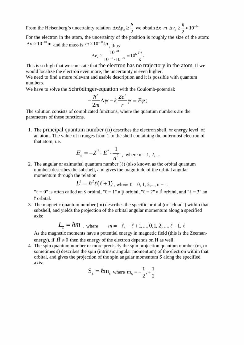
The solution consists of complicated functions, where the quantum numbers are the parameters of these functions. 1. The principal quantum number (n) describes the electron shell, or energy level, of
an atom. The value of n ranges from 1 to the shell containing the outermost electron of that atom, i.e.
2 *2
1n Z E
nΕ = − ⋅ ⋅ , where n = 1, 2, ...
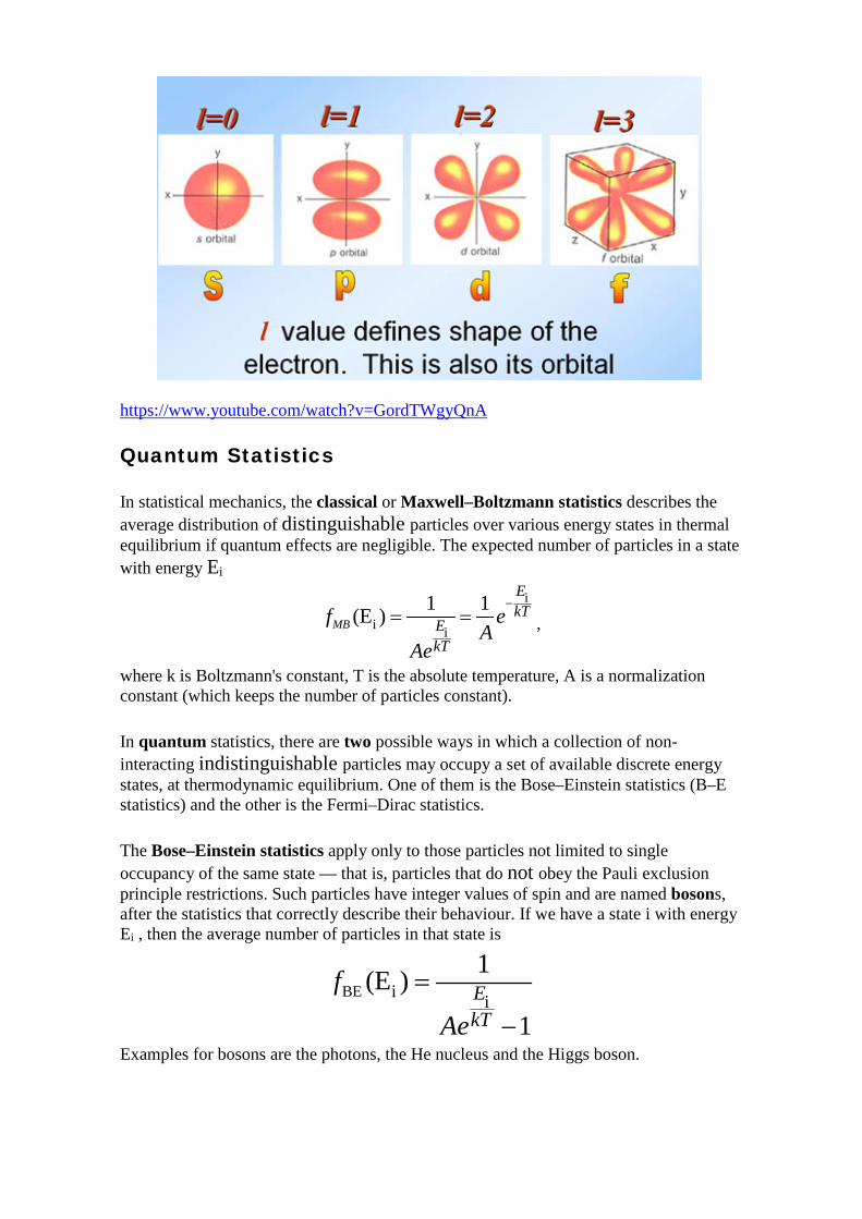
2. The angular or azimuthal quantum number (ℓ) (also known as the orbital quantum number) describes the subshell, and gives the magnitude of the orbital angular momentum through the relation
2 2 ( 1)L = + , where ℓ = 0, 1, 2,..., n − 1. "ℓ = 0" is often called an s orbital, "ℓ = 1" a p orbital, "ℓ = 2" a d orbital, and "ℓ = 3" an f orbital.
3. The magnetic quantum number (m) describes the specific orbital (or "cloud") within that subshell, and yields the projection of the orbital angular momentum along a specified axis:
zL m= , where , 1,...,0,1, 2, ..., 1,m = − − + − As the magnetic moments have a potential energy in magnetic field (this is the Zeeman-energy), if 0H ≠
then the energy of the electron depends on H as well. 4. The spin quantum number or more precisely the spin projection quantum number (ms or
sometimes s) describes the spin (intrinsic angular momentum) of the electron within that orbital, and gives the projection of the spin angular momentum S along the specified axis:
z sS m= where s1 1m ,2 2
= − +
https://www.youtube.com/watch?v=GordTWgyQnA Quantum Statistics In statistical mechanics, the classical or Maxwell–Boltzmann statistics describes the average distribution of distinguishable particles over various energy states in thermal equilibrium if quantum effects are negligible. The expected number of particles in a state with energy Ei
i
i
i
1 1(E )MB
EkT
EkT
f eA
Ae
−= = ,
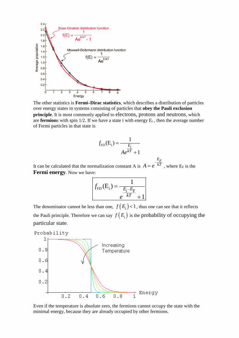
where k is Boltzmann's constant, T is the absolute temperature, A is a normalization constant (which keeps the number of particles constant). In quantum statistics, there are two possible ways in which a collection of non-interacting indistinguishable particles may occupy a set of available discrete energy states, at thermodynamic equilibrium. One of them is the Bose–Einstein statistics (B–E statistics) and the other is the Fermi–Dirac statistics. The Bose–Einstein statistics apply only to those particles not limited to single occupancy of the same state — that is, particles that do not obey the Pauli exclusion principle restrictions. Such particles have integer values of spin and are named bosons, after the statistics that correctly describe their behaviour. If we have a state i with energy Ei , then the average number of particles in that state is
BE i i
1(E )
1EkT
f
Ae
=
−
Examples for bosons are the photons, the He nucleus and the Higgs boson.
The other statistics is Fermi–Dirac statistics, which describes a distribution of particles over energy states in systems consisting of particles that obey the Pauli exclusion principle. It is most commonly applied to electrons, protons and neutrons, which are fermions with spin 1/2. If we have a state i with energy Ei , then the average number of Fermi particles in that state is
FD i i
1(E )
1EkT
f
Ae
=
+
It can be calculated that the normalization constant A is FE
kTA e−
= , where EF is the Fermi energy. Now we have:
FD i Fi
1(E )
1E E
kT
f
e−
=
+
The denominator cannot be less than one, ( )i 1f E < , thus one can see that it reflects
the Pauli principle. Therefore we can say ( )if E is the probability of occupying the particular state.
Even if the temperature is absolute zero, the fermions cannot occupy the state with the minimal energy, because they are already occupied by other fermions.
At low temperatures, bosons can behave very differently than fermions because an unlimited number of them can collect into the same energy state, a phenomenon called "condensation".
If the energy E is much larger than kT, the EkTe term is much greater than 1, thus the
quantum statistics tend to the classical one. Quantum numbers for atoms with more electrons and the periodic table It is very hard to solve the Schrödinger equation if the number of electrons is greater than one. The results will be similar to the case of one electron, but now the quantum numbers have no exact meaning, they describe the behaviour of the electrons only approximately. The most important difference from the one-electron case is that now the energy depends on the angular quantum number:
n, n, +1E <E
The order of the energy levels: 1s, 2s, 2p, 3s, 3p, 4s, 3d, 4p, 5s, 4d, 5p, 6s, 4f, 5d, 6p, 7s, 5f, 6d, 7p
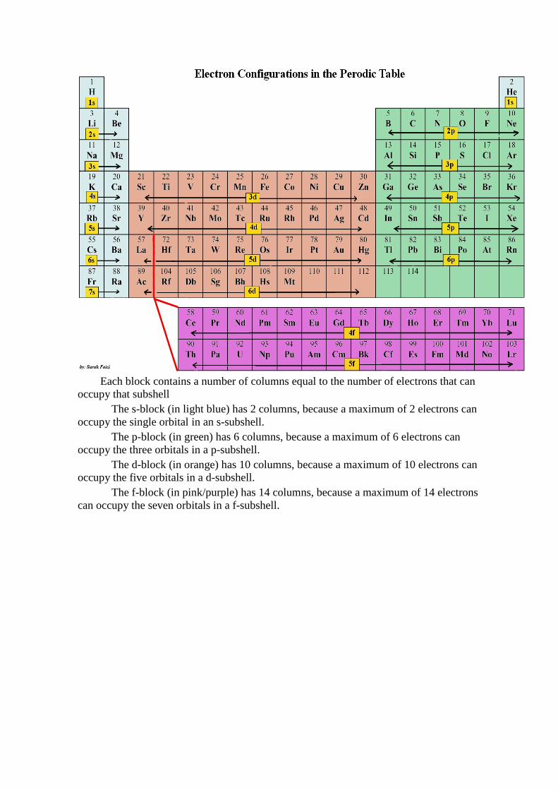
To understand the periodic table, we need the Pauli principle and the energy-minimum principle applied to these concrete energy-levels. An element's location on the periodic table reflects the quantum numbers of the last orbital filled. The period indicates the value of principal quantum number for the valence shell. The lanthanides and actinides, indicated by pink-purple, are in periods 6 and 7, respectively. Each of them contains 14 elements, because if 3= , m has 7 possible values (from -3 to 3), and 2*7=14.
The block indicates the value of the angular quantum number for the last subshell that received electrons in building up the electron configuration. The blocks are named for subshells (s, p, d, f)
Each block contains a number of columns equal to the number of electrons that can occupy that subshell The s-block (in light blue) has 2 columns, because a maximum of 2 electrons can occupy the single orbital in an s-subshell. The p-block (in green) has 6 columns, because a maximum of 6 electrons can occupy the three orbitals in a p-subshell. The d-block (in orange) has 10 columns, because a maximum of 10 electrons can occupy the five orbitals in a d-subshell. The f-block (in pink/purple) has 14 columns, because a maximum of 14 electrons can occupy the seven orbitals in a f-subshell.
Possible elaborative questions:
1) Blackbody radiation 2) Photoelectric effect and the momentum of the photon 3) Line spectra of atoms and the Bohr model 4) Wave particle duality of particles, de-Broglie hypothesis 5) Wave Function and the principle of superposition 6) Operators and eigenvalues 7) The concrete form of the operators and the Schrödinger equation 8) Heisenberg’s uncertainty principle 9) Free particle in 1D 10) Infinite 1D potential well (particle in a box) 11) Solution of Schrödinger equation for a step potential and quantum tunnelling 12) The essence of quantum tunnelling and some examples 13) Angular momentum and atoms with 1 electron 14) Quantum Statistics 15) Atoms with more electrons and the periodic table
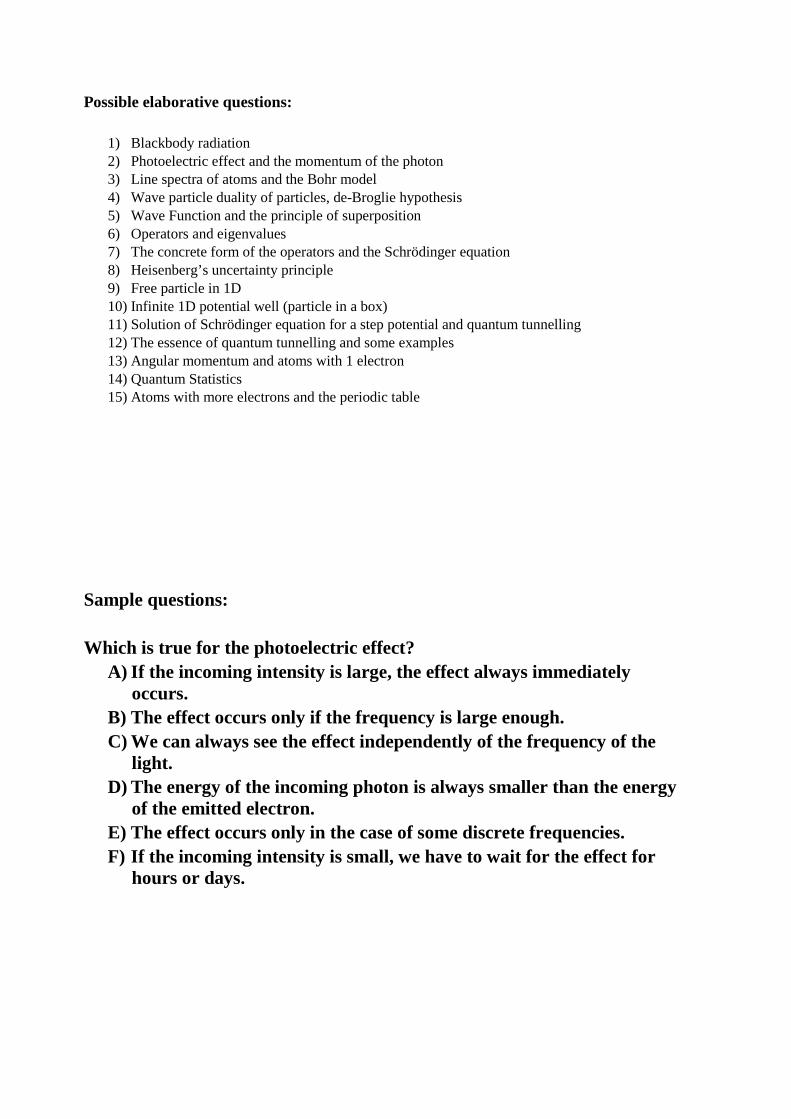
Sample questions: Which is true for the photoelectric effect?
A) If the incoming intensity is large, the effect always immediately occurs.
B) The effect occurs only if the frequency is large enough. C) We can always see the effect independently of the frequency of the
light. D) The energy of the incoming photon is always smaller than the energy
of the emitted electron. E) The effect occurs only in the case of some discrete frequencies. F) If the incoming intensity is small, we have to wait for the effect for
hours or days.
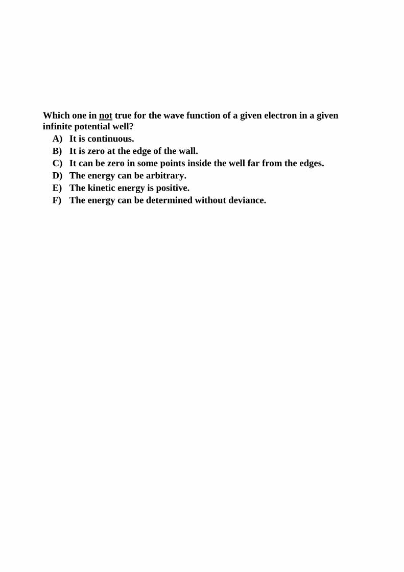
Which one in not true for the wave function of a given electron in a given infinite potential well?
A) It is continuous. B) It is zero at the edge of the wall. C) It can be zero in some points inside the well far from the edges. D) The energy can be arbitrary. E) The kinetic energy is positive. F) The energy can be determined without deviance.


![Connecting Blackbody Radiation, Relativity, and …physics/0605003v1 [physics.class-ph] 28 Apr 2006 Connecting Blackbody Radiation, Relativity, and Discrete Charge in Classical Electrodynamics](https://static.documents.pub/doc/80x56/5abed3837f8b9a3a428d7126/connecting-blackbody-radiation-relativity-and-physics0605003v1-physicsclass-ph.jpg)


