Modern Real Analysis William P. Ziemer with contributions from Monica Torres Department of Mathematics, Indiana University, Bloomington, In- diana E-mail address : [email protected]Department of Mathematics, Purdue University, West Lafayette, Indiana E-mail address : [email protected]
Transcript
Modern Real Analysis
William P. Ziemer
with contributions from Monica Torres
Department of Mathematics, Indiana University, Bloomington, In-
5.1. Elementary Properties of Measurable Functions 125
5.2. Limits of Measurable Functions 136
5.3. Approximation of Measurable Functions 141
Exercises for Chapter 5 145
Chapter 6. Integration 149
6.1. Definitions and Elementary Properties 149
6.2. Limit Theorems 154
6.3. Riemann and Lebesgue Integration–A Comparison 156
6.4. Improper Integrals 159
6.5. Lp Spaces 161
6.6. Signed Measures 169
6.7. The Radon-Nikodym Theorem 174
6.8. The Dual of Lp 180
6.9. Product Measures and Fubini’s Theorem 186
6.10. Lebesgue Measure as a Product Measure 195
6.11. Convolution 197
6.12. Distribution Functions 199
6.13. The Marcinkiewicz Interpolation Theorem 201
Exercises for Chapter 6 206
Chapter 7. Differentiation 219
7.1. Covering Theorems 219
7.2. Lebesgue Points 224
7.3. The Radon-Nikodym Derivative – Another View 228
7.4. Functions of Bounded Variation 233
7.5. The Fundamental Theorem of Calculus 238
7.6. Variation of Continuous Functions 243
7.7. Curve Length 248
7.8. The Critical Set of a Function 255
7.9. Approximate Continuity 260
CONTENTS 5
Exercises for Chapter 7 264
Chapter 8. Elements of Functional Analysis 271
8.1. Normed Linear Spaces 271
8.2. Hahn-Banach Theorem 279
8.3. Continuous Linear Mappings 283
8.4. Dual Spaces 287
8.5. Hilbert Spaces 296
8.6. Weak and Strong Convergence in Lp 306
Exercises for Chapter 8 311
Chapter 9. Measures and Linear Functionals 317
9.1. The Daniell Integral 317
9.2. The Riesz Representation Theorem 325
Exercises for Chapter 9 332
Chapter 10. Distributions 335
10.1. The Space D 335
10.2. Basic Properties of Distributions 340
10.3. Differentiation of Distributions 342
10.4. Essential Variation 347
Exercises for Chapter 10 350
Chapter 11. Functions of Several Variables 353
11.1. Differentiability 353
11.2. Change of Variable 359
11.3. Sobolev Functions 370
11.4. Approximating Sobolev Functions 377
11.5. Sobolev Imbedding Theorem 380
11.6. Applications 384
11.7. Regularity of Weakly Harmonic Functions 386
Exercises for Chapter 11 391
Bibliography 393
Index 395
Preface
This text is an essentially self-contained treatment of material that is normally
found in a first year graduate course in real analysis. Although the presentation is
based on a modern treatment of measure and integration, it has not lost sight of
the fact that the theory of functions of one real variable is the core of the subject.
It is assumed that the student has had a solid course in Advanced Calculus and has
been exposed to rigorous ε, δ arguments. Although the book’s primary purpose is
to serve as a graduate text, we hope that it will also serve as useful reference for
the more experienced mathematician.
The book begins with a chapter on preliminaries and then proceeds with a
chapter on the development of the real number system. This also includes an
informal presentation of cardinal and ordinal numbers. The next chapter provides
the basics of general topological and metric spaces. By the time this chapter has
been concluded, the background of students in a typical course will have been
equalized and they will be prepared to pursue the main thrust of the book.
The text then proceeds to develop measure and integration theory in the next
three chapters. Measure theory is introduced by first considering outer measures
on an abstract space. The treatment here is abstract, yet short, simple, and basic.
By focusing first on outer measures, the development underscores in a natural way
the fundamental importance and significance of σ-algebras. Lebesgue measure,
Lebesgue-Stieltjes measure, and Hausdorff measure are immediately developed as
important, concrete examples of outer measures. Integration theory is presented by
using countably simple functions, that is, functions that assume only a countable
number of values. Conceptually they are no more difficult than simple functions,
but their use leads to a more direct development. Important results such as the
Radon-Nikodym theorem and Fubini’s theorem have received treatments that avoid
some of the usual technical difficulties.
A chapter on elementary functional analysis is followed by one on the Daniell
integral and the Riesz Representation theorem. This introduces the student to a
completely different approach to measure and integration theory. In order for the
student to become more comfortable with this new framework, the linear functional
7
8 PREFACE
approach is further developed by including a short chapter on Schwartz Distribu-
tions. Along with introducing new ideas, this reinforces the student’s previous
encounter with measures as linear functionals. It also maintains connection with
previous material by casting some old ideas in a new light. For example, BV
functions and absolutely continuous functions are characterized as functions whose
distributional derivatives are measures and functions, respectively.
The introduction of Schwartz distributions invites a treatment of functions of
several variables. Since absolutely continuous functions are so important in real
analysis, it is natural to ask whether they have a counterpart among functions of
several variables. In the last chapter, it is shown that this is the case by developing
the class of functions whose partial derivatives (in the sense of distributions) are
functions, thus providing a natural analog of absolutely continuous functions of a
single variable. The analogy is strengthened by proving that these functions are
absolutely continuous in each variable separately. These functions, called Sobolev
functions, are of fundamental importance to many areas of research today. The
chapter is concluded with a glimpse of both the power and the beauty of Dis-
tribution theory by providing a treatment of the Dirichlet Problem for Laplace’s
equation. This presentation is not difficult, but it does call upon many of the top-
ics the student has learned throughout the text, thus providing a fitting end to the
book.
We will use the following notation throughout. The symbol denotes the end
of a proof and a := b means a = b by definition. All theorems, lemmas, corollaries,
definitions, and remarks are numbered as a.b where a denotes the chapter number.
Equation numbers are numbered in a similar way and appear as (a.b). Sections
marked with ∗ are not essential to the main development of the material and may
be omitted.
CHAPTER 1
Preliminaries
1.1. Sets
This is the first of three sections devoted to basic definitions, notation,and terminology used throughout this book. We begin with an elemen-tary and intuitive discussion of sets and deliberately avoid a rigoroustreatment of “set theory” that would take us too far from our mainpurpose.
We shall assume that the notion of set is already known to the reader, at least in
the intuitive sense. Roughly speaking, a set is any identifiable collection of objects
called the elements or members of the set. Sets will usually be denoted by capital
Roman letters such as A, B, C, U, V, . . . , and if an object x is an element of A,
we will write x ∈ A. When x is not an element of A we write x /∈ A. There are
many ways in which the objects of a set may be identified. One way is to display all
objects in the set. For example, x1, x2, . . . , xk is the set consisting of the elements
x1, x2, . . . , xk. In particular, a, b is the set consisting of the elements a and b.
Note that a, b and b, a are the same set. A set consisting of a single element x
is denoted by x and is called a singleton. Often it is possible to identify a set
by describing properties that are possessed by its elements. That is, if P (x) is a
property possessed by an element x, then we write x : P (x) to describe the set
that consists of all objects x for which the property P (x) is true. Obviously, we
have A = x : x ∈ A and x : x 6= x = ∅, the empty set or null set.
The union of sets A and B is the set x : x ∈ A or x ∈ B and this is written
as A ∪B. Similarly, if A is an arbitrary family of sets, the union of all sets in this
family is
(1.1) x : x ∈ A for some A ∈ A
and is denoted by
(1.2)⋃A∈A
A or as⋃A : A ∈ A.
1
2 1. PRELIMINARIES
Sometimes a family of sets will be defined in terms of an indexing set I and then
we write
(1.3) x : x ∈ Aα for some α ∈ I =⋃α∈I
Aα.
If the index set I is the set of positive integers, then we write (1.3) as
(2.1)∞⋃i=1
Ai.
The intersection of sets A and B is defined by x : x ∈ A and x ∈ B and is
written as A ∩B. Similar to (1.1) and (1.2) we have
x : x ∈ A for all A ∈ A =⋂A∈A
A =⋂A : A ∈ A.
A family A of sets is said to be disjoint if A1 ∩ A2 = ∅ for every pair A1 and A2
of distinct members of A.
If every element of the set A is also an element of B, then A is called a subset
of B and this is written as A ⊂ B or B ⊃ A. With this terminology, the possibility
that A = B is allowed. The set A is called a proper subset of B if A ⊂ B and
A 6= B.
The difference of two sets is
A \B = x : x ∈ A and x /∈ B
while the symmetric difference is
A∆B = (A \B) ∪ (B \A).
In most discussions, a set A will be a subset of some underlying space X and
in this context, we will speak of the complement of A (relative to X) as the set
x : x ∈ X and x /∈ A. This set is denoted by A and this notation will be used
if there is no doubt that complementation is taken with respect to X. In case of
possible ambiguity, we write X \ A instead of A. The following identities, known
as de Morgan’s laws, are very useful and easily verified:
(2.2)
( ⋃α∈I
Aα
)∼=⋂α∈I
Aα( ⋂α∈I
Aα
)∼=⋃α∈I
Aα.
We shall denote the set of all subsets of X, called the power set of X, by
P(X). Thus,
(2.3) P(X) = A : A ⊂ X.
1.2. FUNCTIONS 3
The notions of limit superior (lim sup) and lim inferior (lim inf) are
defined for sets as well as for sequences:
(2.4)
lim supi→∞
Ei =∞⋂k=1
∞⋃i=k
Ei
lim infi→∞
Ei =∞⋃k=1
∞⋂i=k
Ei
It is easily seen that
(3.1)
lim supi→∞
Ei = x : x ∈ Ei for infinitely many i ,
lim infi→∞
Ei = x : x ∈ Ei for all but finitely many i .
We use the following notation throughout:
∅ = the empty set,
N = the set of positive integers, (not including zero),
Z = the set of integers,
Q = the set of rational numbers,
R = the set of real numbers.
We assume the reader has knowledge of the sets N,Z, and Q, while R will be
carefully constructed in Section 2.1.
1.2. Functions
In this section an informal discussion of relations and functions is given,a subject that is encountered in several forms in elementary analysis.In this development, we adopt the notion that a relation or function isindistinguishable from its graph.
If X and Y are sets, the Cartesian product of X and Y is
(3.2) X × Y = all ordered pairs (x, y) : x ∈ X, y ∈ Y .
The ordered pair (x, y) is thus to be distinguished from (y, x). We will discuss
the Cartesian product of an arbitrary family of sets later in this section.
A relation from X to Y is a subset of X × Y . If f is a relation, then the
domain and range of f are
domf = X ∩ x : (x, y) ∈ f for some y ∈ Y
rngf = Y ∩ y : (x, y) ∈ f for some x ∈ X .
4 1. PRELIMINARIES
Frequently symbols such as ∼ or ≤ are used to designate a relation. In these
cases the notation x ∼ y or x ≤ y will mean that the element (x, y) is a member of
the relation ∼ or ≤, respectively.
A relation f is said to be single-valued if y = z whenever (x, y) and (x, z) ∈f . A single-valued relation is called a function. The terms mapping, map,
transformation are frequently used interchangeably with function, although the
term function is usually reserved for the case when the range of f is a subset of R.
If f is a mapping and (x, y) ∈ f , we let f(x) denote y. We call f(x) the image of x
under f . We will also use the notation x 7→ f(x), which indicates that x is mapped
to f(x) by f . If A ⊂ X, then the image of A under f is
(4.1) f(A) = y : y = f(x), for some x ∈ domf ∩A.
Also, the inverse image of B under f is
(4.2) f−1(B) = x : x ∈ domf, f(x) ∈ B.
In case the set B consists of a single point y, or in other words B = y, we will
simply write f−1y instead of the full notation f−1(y). If A ⊂ X and f a
mapping with domf ⊂ X, then the restriction of f to A, denoted by f A, is
defined by f A(x) = f(x) for all x ∈ A ∩ domf .
If f is a mapping from X to Y and g a mapping from Y to Z, then the
composition of g with f is a mapping from X to Z defined by
(4.3) g f = (x, z) : (x, y) ∈ f and (y, z) ∈ g for some y ∈ Y .
If f is a mapping such that domf = X and rngf ⊂ Y , then we write f : X → Y .
The mapping f is called an injection or is said to be univalent if f(x) 6= f(x′)
whenever x, x′ ∈ domf with x 6= x′. The mapping f is called a surjection or
onto Y if for each y ∈ Y , there exists x ∈ X such that f(x) = y; in other words,
f is a surjection if f(X) = Y . Finally, we say that f is a bijection if f is both
an injection and a surjection. A bijection f : X → Y is also called a one-to-one
correspondence between X and Y .
There is one relation that is particularly important and is so often encountered
that it requires a separate definition.
4.1. Definition. If X is a set, an equivalence relation on X (often denoted
by ∼) is a relation characterized by the following conditions:
(i) x ∼ x for every x ∈ X (reflexive)
(ii) if x ∼ y, then y ∼ x, (symmetric)
(iii) if x ∼ y and y ∼ z, then x ∼ z. (transitive)
1.2. FUNCTIONS 5
Given an equivalence relation ∼ on X, a subset A of X is called an equivalence
class if and only if there is an element x ∈ A such that A consists precisely of those
elements y such that x ∼ y. One can easily verify that dsitinct equivalence classes
are disjoint and that X can be expressed as the union of equivalence classes.
A sequence in a space X is a mapping f : N→ X. It is convenient to denote
a sequence f as a list. Thus, if f(k) = xk, we speak of the sequence xk∞k=1 or
simply xk. A subsequence is obtained by discarding some elements of the original
sequence and ordering the elements that remain in the usual way. Formally, we say
that xk1 , xk2 , xk3 , . . . , is a subsequence of x1, x2, x3, . . . , if there is a mapping
g : N→ N such that for each i ∈ N, xki = xg(i) and if g(i) < g(j) whenever i < j.
Our final topic in this section is the Cartesian product of a family of sets. Let
X be a family of sets Xα indexed by a set I. The Cartesian product of X is
denoted by ∏α∈I
Xα
and is defined as the set of all mappings
x : I →⋃Xα
with the property that
(5.1) x(α) ∈ Xα
for each α ∈ I. Each mapping x is called a choice mapping for the family X .
Also, we call x(α) the αth coordinate of x. This terminology is perhaps easier
to understand if we consider the case where I = 1, 2, . . . , n. As in the preceding
paragraph, it is useful to denote the choice mapping x as a list x(1), x(2), . . . , x(n),and even more useful if we write x(i) = xi. The mapping x is thus identified with
the ordered n-tuple (x1, x2, . . . , xn). Here, the word “ordered” is crucial because an
n-tuple consisting of the same elements but in a different order produces a different
mapping x. Consequently, the Cartesian product becomes the set of all ordered
n-tuples:
(5.2)
n∏i=1
Xi = (x1, x2, . . . , xn) : xi ∈ Xi, i = 1, 2, . . . , n.
In the special case where Xi = R, i = 1, 2, . . . , n, an element of the Cartesian
product is a mapping that can be identified with an ordered n-tuple of real numbers.
We denote the set of all ordered n-tuples (also referred to as vectors) by
Rn = (x1, x2, . . . , xn) : xi ∈ R, i = 1, 2, . . . , n
6 1. PRELIMINARIES
Rn is called Euclidean n-space. The norm of a vector x is defined as
(6.1) |x| =√x2
1 + x22 + · · ·+ x2
n;
the distance between two vectors x and y is |x− y|. As we mentioned earlier in
this section, the Cartesian product of two sets X1 and X2 is denoted by X1×X2.
6.1. Remark. A fundamental issue that we have not addressed is whether the
Cartesian product of an arbitrary family of sets is nonempty. This involves concepts
from set theory and is the subject of the next section.
1.3. Set Theory
The material discussed in the previous two sections is based on toolsfound in elementary set theory. However, in more advanced areas ofmathematics this material is not sufficient to discuss or even formulatesome of the concepts that are needed. An example of this occurred inthe previous section during the discussion of the Cartesian product ofan arbitrary family of sets. Indeed, the Cartesian product of familiesof sets requires the notion of a choice mapping whose existence is notobvious. Here, we give a brief review of the Axiom of Choice and someof its logical equivalences.
A fundamental question that arises in the definition of the Cartesian product of an
arbitrary family of sets is the existence of choice mappings. This is an example of
a question that cannot be answered within the context of elementary set theory.
In the beginning of the 20th century, Ernst Zermelo formulated an axiom of set
theory called the Axiom of Choice, which asserts that the Cartesian product of an
arbitrary family of nonempty sets exists and is nonempty. The formal statement is
as follows.
6.2. The Axiom of Choice. If Xα is a nonempty set for each element α of
an index set I, then ∏α∈I
Xα
is nonempty.
6.3. Proposition. The following statement is equivalent to the Axiom of Choice:
If Xαα∈A is a disjoint family of nonempty sets, then there is a set S ⊂ ∪α∈AXα
such that S ∩Xα consists of precisely one element for every α ∈ A.
Proof. The Axiom of Choice states that there exists f : A → ∪α∈AXα such
that f(α) ∈ Xα for each α ∈ A. The set S := f(A) satisfies the conclusion of the
statement. Conversely, if such a set S exists, then the mapping Af−→ ∪α∈AXα
defined by assigning the point S ∩Xα the value of f(α) implies the validity of the
Axiom of Choice.
1.3. SET THEORY 7
7.1. Definition. Given a set S and a relation ≤ on S, we say that ≤ is a
partial ordering if the following three conditions are satisfied:
(i) x ≤ x for every x ∈ S (reflexive)
(ii) if x ≤ y and y ≤ x, then x = y, (antisymmetric)
(iii) if x ≤ y and y ≤ z, then x ≤ z. (transitive)
If, in addition,
(iv) either x ≤ y or y ≤ x, for all x, y ∈ S, (trichotomy)
then ≤ is called a linear or total ordering.
For example, Z is linearly ordered with its usual ordering, whereas the family
of all subsets of a given set X is partially ordered (but not linearly ordered) by ⊂.
If a set X is endowed with a linear ordering, then each subset A of X inherits the
ordering of X. That is, the restriction to A of the linear ordering on X induces a
linear ordering on A. The following two statements are known to be equivalent to
the Axiom of Choice.
7.2. Hausdorff Maximal Principle. Every partially ordered set has a max-
imal linearly ordered subset.
7.3. Zorn’s Lemma. If X is a partially ordered set with the property that each
linearly ordered subset has an upper bound, then X has a maximal element. In
particular, this implies that if E is a family of sets (or a collection of families of
sets) and if ∪F : F ∈ F ∈ E for any subfamily F of E with the property that
F ⊂ G or G ⊂ F whenever F,G ∈ F ,
then there exists E ∈ E , which is maximal in the sense that it is not a subset of any
other member of E.
In the following, we will consider other formulations of the Axiom of Choice.
This will require the notion of a linear ordering on a set.
A non-empty set X endowed with a linear order is said to be well-ordered
if each subset of X has a first element with respect to its induced linear order.
Thus, the integers, Z, with the usual ordering is not a well-ordered set, whereas
the set N is well-ordered. However, it is possible to define a linear ordering on Zthat produces a well-ordering. In fact, it is possible to do this for an arbitrary set
if we assume the validity of the Axiom of Choice. This is stated formally in the
Well-Ordering Theorem.
7.4. Theorem (The Well-Ordering Theorem). Every set can be well-ordered.
That is, if A is an arbitrary set, then there exists a linear ordering of A with the
property that each non-empty subset of A has a first element.
8 1. PRELIMINARIES
Cantor put forward the continuum hypothesis in 1878, conjecturing that every
infinite subset of the continuum is either countable (i.e. can be put in 1-1 corre-
spondence with the natural numbers) or has the cardinality of the continuum (i.e.
can be put in 1-1 correspondence with the real numbers). The importance of this
was seen by Hilbert who made the continuum hypothesis the first in the list of
problems which he proposed in his Paris lecture of 1900. Hilbert saw this as one of
the most fundamental questions which mathematicians should attack in the 1900s
and he went further in proposing a method to attack the conjecture. He suggested
that first one should try to prove another of Cantor’s conjectures, namely that any
set can be well ordered.
Zermelo began to work on the problems of set theory by pursuing, in particular,
Hilbert’s idea of resolving the problem of the continuum hypothesis. In 1902 Zer-
melo published his first work on set theory which was on the addition of transfinite
cardinals. Two years later, in 1904, he succeeded in taking the first step suggested
by Hilbert towards the continuum hypothesis when he proved that every set can
be well ordered. This result brought fame to Zermelo and also earned him a quick
promotion; in December 1905, he was appointed as professor in Gottingen.
The axiom of choice is the basis for Zermelo’s proof that every set can be well
ordered; in fact the axiom of choice is equivalent to the well ordering property so we
now know that this axiom must be used. His proof of the well ordering property used
the axiom of choice to construct sets by transfinite induction. Although Zermelo
certainly gained fame for his proof of the well ordering property, set theory at this
time was in the rather unusual position that many mathematicians rejected the type
of proofs that Zermelo had discovered. There were strong feelings as to whether
such non-constructive parts of mathematics were legitimate areas for study and
Zermelo’s ideas were certainly not accepted by quite a number of mathematicians.
The fundamental discoveries of K. Godel [4] and P. J. Cohen [2], [3] shook
the foundations of mathematics with results that placed the axiom of choice in a
very interesting position. Their work shows that the Axiom of Choice, in fact, is
a new principle in set theory because it can neither be proved nor disproved from
the usual Zermelo-Fraenkel axioms of set theory. Indeed, Godel showed, in 1940,
that the Axiom of Choice cannot be disproved using the other axioms of set theory
and then in 1963, Paul Cohen proved that the Axiom of Choice is independent of
the other axioms of set theory. The importance of the Axiom of Choice will readily
be seen throughout the following development, as we appeal to it in a variety of
contexts.
EXERCISES FOR CHAPTER 1 9
Exercises for Chapter 1
Section 1.1
1.1 Two sets are identical if and only if they have the same members. That is,
A = B if and only if for each element x, x ∈ A when and only when x ∈ B.
Prove A = B if and only if A ⊂ B and B ⊂ A. that A ⊂ B if and only if
B = A ∪B. Prove de Morgan’s laws, 2.2.
1.2 Let Ei, i = 1, 2, . . . , be a family of sets. Use definitions (2.4) to prove
lim infi→∞
Ei ⊂ lim supi→∞
Ei
Section 1.2
1.3 Prove that f (g h) = (f g) h for mappings f, g, and h.
1.4 Prove that (f g)−1(A) = g−1[f−1(A)] for mappings f and g and an arbitrary
set A.
1.5 Prove: If f : X → Y is a mapping and A ⊂ B ⊂ X, then f(A) ⊂ f(B) ⊂ Y .
Also, prove that if E ⊂ F ⊂ Y , then f−1(E) ⊂ f−1(F ) ⊂ X.
1.6 Prove: If A ⊂ P(X), then
f( ⋃A∈A
A)
=⋃A∈A
f(A) and f( ⋂A∈A
A)⊂⋂A∈A
f(A).
and
f−1( ⋃A∈A
A)
=⋃A∈A
f−1(A) and f−1( ⋂A∈A
A)
=⋂A∈A
f−1(A).
Give an example that shows the above inclusion cannot be replaced by equality.
1.7 Consider a nonempty set X and its power set P(X). For each x ∈ X, let
Bx = 0, 1 and consider the Cartesian product∏x∈X Bx. Exhibit a natural
one-to-one correspondence between P(X) and∏x∈X Bx.
1.8 Let Xf−→ Y be an arbitrary mapping and suppose there is a mapping Y
g−→ X
such that f g(y) = y for all y ∈ Y and that g f(x) = x for all x ∈ X. Prove
that f is one-to-one from X onto Y and that g = f−1.
1.9 Show that A × (B ∪ C) = (A × B) ∪ (A × C). Also, show that in general
A ∪ (B × C) 6= (A ∪B)× (A ∪ C).
Section 1.3
1.10 Use a one-to-one correspondence between Z and N to exhibit a linear ordering
of N that is not a well-ordering.
1.11 Use the natural partial ordering of P(1, 2, 3) to exhibit a partial
1.12 For (a, b), (c, d) ∈ N×N, define (a, b) ≤ (c, d) if either a < c or a = c and b ≤ d.
With this relation, prove that N× N is a well-ordered set.
10 1. PRELIMINARIES
1.13 Let P denote the space of all polynomials defined on R. For p1, p2 ∈ P , define
p1 ≤ p2 if there exists x0 such that p1(x) ≤ p2(x) for all x ≥ x0. Is ≤ a linear
ordering? Is P well ordered?
1.14 Let C denote the space of all continuous functions on [0, 1]. For f1, f2 ∈ C,
define f1 ≤ f2 if f1(x) ≤ f2(x) for all x ∈ [0, 1]. Is ≤ a linear ordering? Is C
well ordered?
1.15 Prove that the following assertion is equivalent to the Axiom of Choice: If A
and B are nonempty sets and f : A → B is a surjection (that is, f(A) = B),
then there exists a function g : B → A such that g(y) ∈ f−1(y) for each y ∈ B.
1.16 Use the following outline to prove that for any two sets A and B, either cardA ≤cardB or cardB ≤ cardA: Let F denote the family of all injections from
subsets of A into B. Since F can be considered as a family of subsets of A×B,
it can be partially ordered by inclusion. Thus, we can apply Zorn’s lemma
to conclude that F has a maximal element, say f . If a ∈ A \ domain f and
b ∈ B \ f(A), then extend f to A ∪ a by defining f(a) = b. Then f remains
an injection and thus contradicts maximality. Hence, either domain f = A in
which case cardA ≤ cardB or B = range f in which case f−1 is an injection
from B into A, which would imply cardB ≤ cardA.
1.17 Complete the details of the following proposition: If cardA ≤ cardB and
cardB ≤ cardA, then cardA = cardB.
Let f : A → B and g : B → A be injections. If a ∈ A ∩ range g, we have
g−1(a) ∈ B. If g−1(a) ∈ rangef , we have f−1(g−1(a)) ∈ A. Continue this
process as far as possible. There are three possibilities: either the process
continues indefinitely, or it terminates with an element of A \ range g (possibly
with a itself) or it terminates with an element of B \ range f . These three cases
determine disjoint sets A∞, AA and AB whose union is A. In a similar manner,
B can be decomposed into B∞, BB and BA. Now f maps A∞ onto B∞ and
AA onto BA and g maps BB onto AB . If we define h : A→ B by h(a) = f(a)
if a ∈ A∞ ∪AA and h(a) = g−1(a) if a ∈ AB , we find that h is injective.
CHAPTER 2
Real, Cardinal and Ordinal Numbers
2.1. The Real Numbers
A brief development of the construction of the Real Numbers is given interms of equivalence classes of Cauchy sequences of rational numbers.This construction is based on the assumption that properties of therational numbers, including the integers, are known.
In our development of the real number system, we shall assume that properties of
the natural numbers, integers, and rational numbers are known. In order to agree
on what the properties are, we summarize some of the more basic ones. Recall that
the natural numbers are designated as
N : = 1, 2, . . . , k, . . ..
They form a well-ordered set when endowed with the usual ordering. The order-
ing on N satisfies the following properties:
(i) x ≤ x for every x ∈ S.
(ii) if x ≤ y and y ≤ x, then x = y.
(iii) if x ≤ y and y ≤ z, then x ≤ z.(iv) for all x, y ∈ S, either x ≤ y or y ≤ x.
The four conditions above define a linear ordering on S, a topic that was in-
troduced in Section 1.3 and will be discussed in greater detail in Section 2.3. The
linear order ≤ of N is compatible with the addition and multiplication operations
in N. Furthermore, the following three conditions are satisfied:
(i) Every nonempty subset of N has a first element; i.e., if ∅ 6= S ⊂ N, there is an
element x ∈ S such that x ≤ y for any element y ∈ S. In particular, the set Nitself has a first element that is unique, in view of (ii) above, and is denoted
by the symbol 1,
(ii) Every element of N, except the first, has an immediate predecessor. That is,
if x ∈ N and x 6= 1, then there exists y ∈ N with the property that y ≤ x and
z ≤ y whenever z ≤ x.
(iii) N has no greatest element; i.e., for every x ∈ N, there exists y ∈ N such that
x 6= y and x ≤ y.
11
12 2. REAL, CARDINAL AND ORDINAL NUMBERS
The reader can easily show that (i) and (iii) imply that each element of N has
an immediate successor, i.e., that for each x ∈ N, there exists y ∈ N such that
x < y and that if x < z for some z ∈ N where y 6= z, then y < z. The immediate
successor of x, y, will be denoted by x′. A nonempty set S ⊂ N is said to be finite
if S has a greatest element.
From the structure established above follows an extremely important result,
the so-called principle of mathematical induction, which we now prove.
12.1. Theorem. Suppose S ⊂ N is a set with the property that 1 ∈ S and that
x ∈ S implies x′ ∈ S. Then S = N.
Proof. Suppose S is a proper subset of N that satisfies the hypotheses of
the theorem. Then N \ S is a nonempty set and therefore by (i) above, has a
first element x. Note that x 6= 1 since 1 ∈ S. From (ii) we see that x has an
immediate predecessor, y. As y ∈ S, we have y′ ∈ S. Since x = y′, we have x ∈ S,
contradicting the choice of x as the first element of N \ S.
Also, we have x ∈ S since x = y′. By definition, x is the first element of N−S,
thus producing a contradiction. Hence, S = N.
The rational numbers Q may be constructed in a formal way from the natural
numbers. This is accomplished by first defining the integers, both negative and
positive, so that subtraction can be performed. Then the rationals are defined
using the properties of the integers. We will not go into this construction but
instead leave it to the reader to consult another source for this development. We
list below the basic properties of the rational numbers.
The rational numbers are endowed with the operations of addition and multi-
plication that satisfy the following conditions:
(i) For every r, s ∈ Q, r + s ∈ Q, and rs ∈ Q.(ii) Both operations are commutative and associative, i.e., r + s = s + r, rs =
sr, (r + s) + t = r + (s+ t), and (rs)t = r(st).
(iii) The operations of addition and multiplication have identity elements 0 and 1
respectively, i.e., for each r ∈ Q, we have
0 + r = r and 1 · r = r.
(iv) The distributive law is valid:
r(s+ t) = rs+ rt
whenever r, s, and t are elements of Q.
(v) The equation r + x = s has a solution for every r, s ∈ Q. The solution is
denoted by s− r.
2.1. THE REAL NUMBERS 13
(vi) The equation rx = s has a solution for every r, s ∈ Q with r 6= 0. This solution
is denoted by s/r. Any algebraic structure satisfying the six conditions above
is called a field; in particular, the rational numbers form a field. The set Qcan also be endowed with a linear ordering. The order relation is related to
the operations of addition and multiplication as follows:
(vii) If r ≥ s, then for every t ∈ Q, r + t ≥ s+ t.
(viii) 0 < 1.
(ix) If r ≥ s and t ≥ 0, then rt ≥ st.
The rational numbers thus provides an example of an ordered field. The proof of
the following is elementary and is left to the reader, see Exercise 2.6.
13.1. Theorem. Every ordered field F contains an isomorphic image of Q and
the isomorphism can be taken as order preserving.
In view of this result, we may view Q as a subset of F . Consequently, the
following definition is meaningful.
13.2. Definition. An ordered field F is called an Archimedean ordered field,
if for each a ∈ F and each positive b ∈ Q, there exists a positive integer n such
that nb > a. Intuitively, this means that no matter how large a is and how small
b, successive repetitions of b will eventually exceed a.
Although the rational numbers form a rich algebraic system, they are inade-
quate for the purposes of analysis because they are, in a sense, incomplete. For
example, not every positive rational number has a rational square root. We now
proceed to construct the real numbers assuming knowledge of the integers and ra-
tional numbers. This is basically an assumption concerning the algebraic structure
of the real numbers.
The linear order structure of the field permits us to define the notion of the
absolute value of an element of the field. That is, the absolute value of x is
defined by
|x| =
x if x ≥ 0
−x if x < 0.
We will freely use properties of the absolute value such as the triangle inequality in
our development.
The following two definitions are undoubtedly well known to the reader; we
state them only to emphasize that at this stage of the development, we assume
knowledge of only the rational numbers.
14 2. REAL, CARDINAL AND ORDINAL NUMBERS
14.1. Definition. A sequence of rational numbers ri is Cauchy if and only
if for each rational ε > 0, there exists a positive integer N(ε) such that |ri− rk| < ε
whenever i, k ≥ N(ε).
14.2. Definition. A rational number r is said to be the limit of a sequence of
rational numbers ri if and only if for each rational ε > 0, there exists a positive
integer N(ε) such that
|ri − r| < ε
for i ≥ N(ε). This is written as
limi→∞
ri = r
and we say that ri converges to r.
We leave the proof of the following proposition to the reader.
14.3. Proposition. A sequence of rational numbers that converges to a rational
number is Cauchy.
14.4. Proposition. A Cauchy sequence of rational numbers, ri, is bounded.
That is, there exists a rational number M such that |ri| ≤M for i = 1, 2, . . . .
Proof. Choose ε = 1. Since the sequence ri is Cauchy, there exists a
positive integer N such that
|ri − rj | < 1 whenever i, j ≥ N.
In particular, |ri−rN | < 1 whenever i ≥ N . By the triangle inequality, |ri|−|rN | ≤|ri − rN | and therefore,
|ri| < |rN |+ 1 for all i ≥ N.
If we define
M = Max|r1|, |r2|, . . . , |rN−1|, |rN |+ 1
then |ri| ≤M for all i ≥ 1.
The reader can easily provide a proof of the following.
14.5. Proposition. Every Cauchy sequence of rational numbers has at most
one limit.
The fact that some Cauchy sequences in Q may not have a limit (in Q) is what
makes Q incomplete. We will construct the completion by means of equivalence
classes of Cauchy sequences.
2.1. THE REAL NUMBERS 15
14.6. Definition. Two Cauchy sequences of rational numbers ri and siare said to be equivalent if and only if
limi→∞
(ri − si) = 0.
We write ri ∼ si when ri and si are equivalent. It is easy to show
that this, in fact, is an equivalence relation. That is,
(i) ri ∼ ri, (reflexivity)
(ii) ri ∼ si if and only if si ∼ ri, (symmetry)
(iii) if ri ∼ si and si ∼ ti, then ri ∼ ti. (transitivity)
The set of all Cauchy sequences of rational numbers equivalent to a fixed Cauchy
sequence is called an equivalence class of Cauchy sequences. The fact that we
are dealing with an equivalence relation implies that the set of all Cauchy sequences
of rational numbers is partitioned into mutually disjoint equivalence classes. For
each rational number r, the sequence each of whose values is r (i.e., the constant
sequence) will be denoted by r. Hence, 0 is the constant sequence whose values are
0. This brings us to the definition of a real number.
15.1. Definition. An equivalence class of Cauchy sequences of rational num-
bers is termed a real number. In this section, we will usually denote real numbers
by ρ, σ, etc. With this convention, a real number ρ designates an equivalence class
of Cauchy sequences, and if this equivalence class contains the sequence ri, we
will write
ρ = ri
and say that ρ is represented by ri. Note that 1/i∞i=1 ∼ 0 and that every ρ has
a representative ri∞i=1 with ri 6= 0 for every i.
In order to define the sum and product of real numbers, we invoke the corre-
sponding operations on Cauchy sequences of rational numbers. This will require
the next two elementary propositions whose proofs are left to the reader.
15.2. Proposition. If ri and si are Cauchy sequences of rational numbers,
then ri ± si and ri · si are Cauchy sequences. The sequence ri/si is also
Cauchy provided si 6= 0 for every i and si∞i=1 6∼ 0.
15.3. Proposition. If ri ∼ r′i and si ∼ s′i , then ri± si ∼ r′i± s′iand ri · si ∼ r′i · s′i. Similarly, ri/si ∼ r′i/s′i provided si 6∼ 0, and si 6= 0
and s′i 6= 0 for every i.
16 2. REAL, CARDINAL AND ORDINAL NUMBERS
16.1. Definition. If ρ and σ are represented by ri and si respectively, then
ρ± σ is defined by the equivalence class containing ri ± si and ρ · σ by ri · si.ρ/σ is defined to be the equivalence class containing ri/s′i where si ∼ s′i and
s′i 6= 0 for all i, provided si 6∼ 0.
Reference to Propositions 15.2 and 15.3 shows that these operations are well-
defined. That is, if ρ′ and σ′ are represented by r′i and s′i, where ri ∼ r′iand si ∼ s′i, then ρ+ σ = ρ′ + σ′ and similarly for the other operations.
Since the rational numbers form a field, it is clear that the real numbers also
form a field. However, we wish to show that they actually form an Archimedean
ordered field. For this we first must define an ordering on the real numbers that
is compatible with the field structure; this will be accomplished by the following
theorem.
16.2. Theorem. If ri and si are Cauchy, then one (and only one) of the
following occurs:
(i) ri ∼ si.(ii) There exist a positive integer N and a positive rational number k such that
ri > si + k for i ≥ N .
(iii) There exist a positive integer N and positive rational number k such that
si > ri + k for i ≥ N.
Proof. Suppose that (i) does not hold. Then there exists a rational number
k > 0 with the property that for every positive integer N there exists an integer
i ≥ N such that
|ri − si| > 2k.
This is equivalent to saying that
|ri − si| > 2k for infinitely many i ≥ 1.
Since ri is Cauchy, there exists a positive integer N such that
|ri − rj | < k/2 for all i, j ≥ N1.
Likewise, there exists a positive integer N2 such that
|si − sj | < k/2 for all i, j ≥ N2.
Let N∗ ≥ maxN1, N2 be an integer with the property that
|rN∗ − sN∗ | > 2k.
2.1. THE REAL NUMBERS 17
Either rN∗ > sN∗ or sN∗ > rN∗ . We will show that the first possibility leads to
conclusion (ii) of the theorem. The proof that the second possibility leads to (iii)
is similar and will be omitted. Assuming now that rN∗ > sN∗ , we have
rN∗ > sN∗ + 2k.
It follows from (12.1) and (14.1) that
|rN∗ − ri| < k/2 and |sN∗ − si| < k/2 for all i ≥ N∗.
From this and (14.3) we have that
ri > rN∗ − k/2 > sN∗ + 2k − k/2 = sN∗ + 3k/2 for i ≥ N∗.
But sN∗ > si − k/2 for i ≥ N∗ and consequently,
ri > si + k for i ≥ N∗.
17.1. Definition. If ρ = ri and σ = si, then we say that ρ < σ if there
exist rational numbers q1 and q2 with q1 < q2 and a positive integer N such that
such that ri < q1 < q2 < si for all i with i ≥ N . Note that q1 and q2 can be chosen
to be independent of the representative Cauchy sequences of rational numbers that
determine ρ and σ.
In view of this definition, Theorem 16.2 implies that the real numbers are
comparable, which we state in the following corollary.
17.2. Theorem. Corollary If ρ and σ are real numbers, then one (and only
one) of the following must hold:
(1) ρ = σ,
(2) ρ < σ,
(3) ρ > σ.
Moreover, R is an Archimedean ordered field.
The compatibility of ≤ with the field structure of R follows from Theorem
16.2. That R is Archimedean follows from Theorem 16.2 and the fact that Q is
Archimedean. Note that the absolute value of a real numbr can thus be defined
analogously to that of a rational number.
17.3. Definition. If ρi∞i=1 is a sequence in R and ρ ∈ R we define
limi→∞
ρi = ρ
18 2. REAL, CARDINAL AND ORDINAL NUMBERS
to mean that given any real number ε > 0 there is a positive integer N such that
|ρi − ρ| < ε whenever i ≥ N.
17.4. Remark. Having shown that R is an Archimedean ordered field, we now
know that Q has a natural injection into R by way of the constant sequences. That
is, if r ∈ Q, then the constant sequence r gives its corresponding equivalence class
in R. Consequently, we shall consider Q to be a subset of R, that is, we do not
distinguish between r and its corresponding equivalence class. Moreover, if ρ1 and
ρ2 are in R with ρ1 < ρ2, then there is a rational number r such that ρ1 < r < ρ2.
The next proposition provides a connection between Cauchy sequences in Qwith convergent sequences in R.
18.1. Theorem. If ρ = ri, then
limi→∞
ri = ρ.
Proof. Given ε > 0, we must show the existence of a positive integer N such
that |ri − ρ| < ε whenever i ≥ N . Let ε be represented by the rational sequence
εi. Since ε > 0, we know from Theorem (16.2), (ii), that there exist a positive
rational number k and an integer N1 such that εi > k for all i ≥ N1. Because
the sequence ri is Cauchy, we know there exists a positive integer N2 such that
|ri − rj | < k/2 whenever i, j ≥ N2. Fix an integer i ≥ N2 and let ri be determined
by the constant sequence ri, ri, .... Then the real number ρ− ri is determined by
the Cauchy sequence rj − ri, that is
ρ− ri = rj − ri.
If j ≥ N2, then |rj − ri| < k/2. Note that the real number |ρ − ri| is determined
by the sequence |rj − ri|. Now, the sequence |rj − ri| has the property that
|rj − ri| < k/2 < k < εj for j ≥ max(N1, N2). Hence, by Definition (17.1),
|ρ− ri| < ε. The proof is concluded by taking N = max(N1, N2).
18.2. Theorem. The set of real numbers is complete; that is, every Cauchy
sequence of real numbers converges to a real number.
Proof. Let ρi be a Cauchy sequence of real numbers and let each ρi be
determined by the Cauchy sequence of rational numbers, ri,k∞k=1. By the previous
proposition,
limk→∞
ri,k = ρi.
Thus, for each positive integer i, there exists ki such that
(18.1) |ri,ki − ρi| <1
i.
2.1. THE REAL NUMBERS 19
Let si = ri,ki . The sequence si is Cauchy because
|si − sj | ≤ |si − ρi|+ |ρi − ρj |+ |ρj − sj |
≤ 1/i+ |ρi − ρj |+ 1/j.
Indeed, for ε > 0, there exists a positive integer N > 4/ε such that i, j ≥ N implies
|ρi − ρj | < ε/2. This, along with (18.1), shows that |si − sj | < ε for i, j ≥ N .
Moreover, if ρ is the real number determined by si, then
|ρ− ρi| ≤ |ρ− si|+ |si − ρi|
≤ |ρ− si|+ 1/i.
For ε > 0, we invoke Theorem 18.1 for the existence of N > 2/ε such that the first
term is less than ε/2 for i ≥ N . For all such i, the second term is also less than
ε/2.
The completeness of the real numbers leads to another property that is of basic
importance.
19.1. Definition. A number M is called an upper bound for for a set A ⊂ Rif a ≤ M for all a ∈ A. An upper bound b for A is called a least upper bound
for A if b is less than all other upper bounds for A. The term supremum of A
is used interchangeably with least upper bound and is written supA. The terms
lower bound, greatest lower bound, and infimum are defined analogously.
19.2. Theorem. Let A ⊂ R be a nonempty set that is bounded above (below).
Then supA (infA) exists.
Proof. Let b ∈ R be any upper bound for A and let a ∈ A be an arbitrary
element. Further, using the Archimedean property of R, let M and −m be positive
integers such that M > b and −m > −a, so that we have m < a ≤ b < M . For
each positive integer p let
Ip =
k : k an integer and
k
2pis an upper bound for A
.
Since A is bounded above, it follows that Ip is not empty. Furthermore, if a ∈ Ais an arbitrary element, there is an integer j that is less than a. If k is an integer
such that k ≤ 2pj, then k is not an element of Ip, thus showing that Ip is bounded
20 2. REAL, CARDINAL AND ORDINAL NUMBERS
below. Therefore, since Ip consists only of integers, it follows that Ip has a first
element, call it kp. Because2kp2p+1
=kp2p,
the definition of kp+1 implies that kp+1 ≤ 2kp. But
2kp − 2
2p+1=kp − 1
2p
is not an upper bound for A, which implies that kp+1 6= 2kp − 2. In fact, it follows
that kp+1 > 2kp − 2. Therefore, either
kp+1 = 2kp or kp+1 = 2kp − 1.
Defining ap =kp2p
, we have either
ap+1 =2kp2p+1
= ap or ap+1 =2kp − 1
2p+1= ap −
1
2p+1,
and hence,
ap+1 ≤ ap with ap − ap+1 ≤1
2p+1
for each positive integer p. If q > p ≥ 1, then
0 ≤ ap − aq = (ap − ap+1) + (ap+1 − ap+2) + · · ·+ (aq−1 − aq)
≤ 1
2p+1+
1
2p+2+ · · ·+ 1
2q
=1
2p+1
(1 +
1
2+ · · ·+ 1
2q−p−1
)<
1
2p+1(2) =
1
2p.
Thus, whenever q > p ≥ 1, we have |ap − aq| < 12p , which implies that ap is a
Cauchy sequence. By the completeness of the real numbers, Theorem 18.2, there
is a real number c to which the sequence converges.
We will show that c is the supremum of A. First, observe that c is an upper
bound for A since it is the limit of a decreasing sequence of upper bounds. Secondly,
it must be the least upper bound, for otherwise, there would be an upper bound c′
with c′ < c. Choose an integer p such that 1/2p < c− c′. Then
ap −1
2p≥ c− 1
2p> c+ c′ − c = c′,
which shows that ap− 12p is an upper bound for A. But the definition of ap implies
that
ap −1
2p=kp − 1
2p,
2.2. CARDINAL NUMBERS 21
a contradiction, sincekp − 1
2pis not an upper bound for A.
The existence of inf A in case A is bounded below follows by an analogous
argument.
A linearly ordered field is said to have the least upper bound property if
each nonempty subset that has an upper bound has a least upper bound (in the
field). Hence, R has the least upper bound property. It can be shown that every lin-
early ordered field with the least upper bound property is a complete Archimedean
ordered field. We will not prove this assertion.
2.2. Cardinal Numbers
There are many ways to determine the “size” of a set, the most basicbeing the enumeration of its elements when the set is finite. When theset is infinite, another means must be employed; the one that we use isnot far from the enumeration concept.
21.1. Definition. Two sets A and B are said to be equivalent if there exists
a bijection f : A → B, and then we write A ∼ B. In other words, there is a
one-to-one correspondence between A and B. It is not difficult to show that this
notion of equivalence defines an equivalence relation as described in Definition 4.1
and therefore sets are partitioned into equivalence classes. Two sets in the same
equivalence class are said to have the same cardinal number or to be of the same
cardinality. The cardinal number of a set A is denoted by cardA; that is, cardA is
the symbol we attach to the equivalence class containing A. There are some sets so
frequently encountered that we use special symbols for their cardinal numbers. For
example, the cardinal number of the set 1, 2, . . . , n is denoted by n, cardN = ℵ0,
and cardR = c.
21.2. Definition. A set A is finite if cardA = n for some nonnegative integer
n. A set that is not finite is called infinite. Any set equivalent to the positive
integers is said to be denumerable. A set that is either finite or denumerable is
called countable; otherwise it is called uncountable.
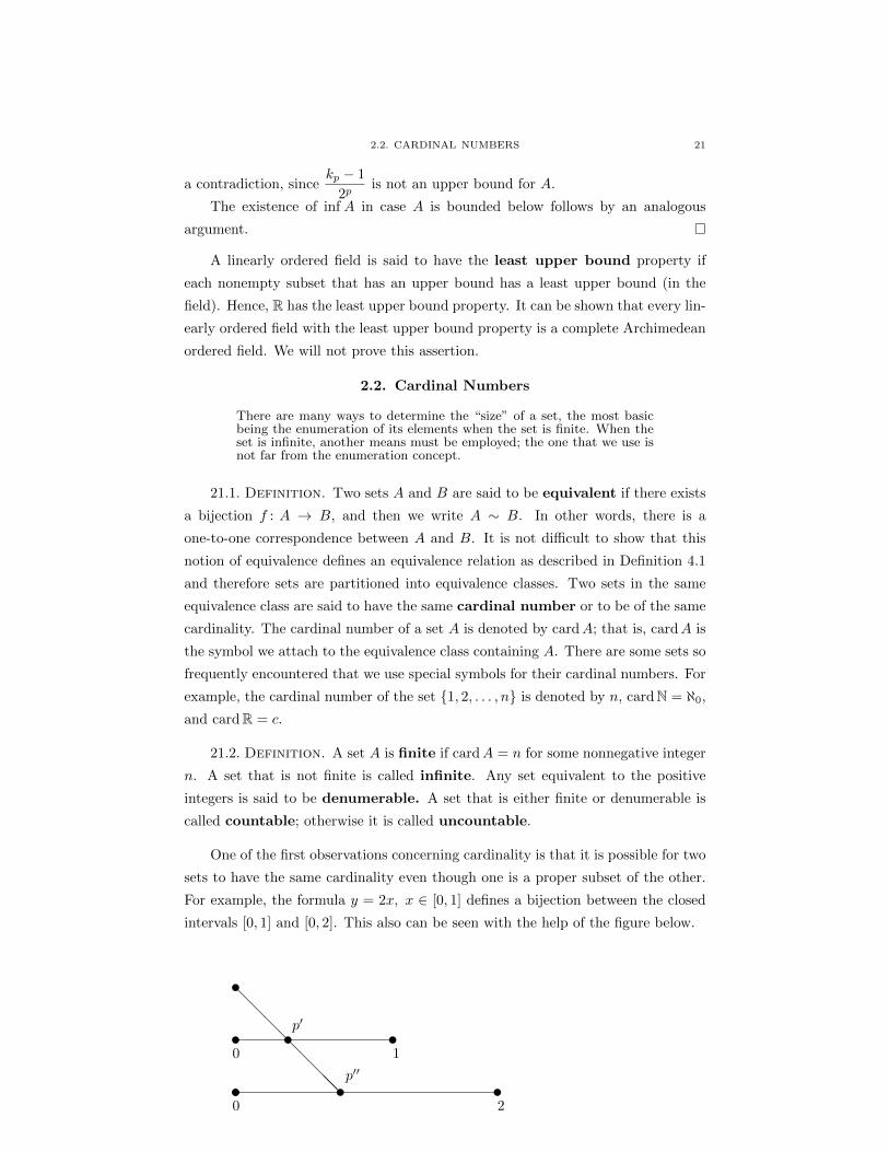
One of the first observations concerning cardinality is that it is possible for two
sets to have the same cardinality even though one is a proper subset of the other.
For example, the formula y = 2x, x ∈ [0, 1] defines a bijection between the closed
intervals [0, 1] and [0, 2]. This also can be seen with the help of the figure below.
tt t tt t
@@@@@@@@t t
0
p′
p′′
0
1
2
22 2. REAL, CARDINAL AND ORDINAL NUMBERS
Another example, utilizing a two-step process, establishes the equivalence be-
tween points x of (−1, 1) and y of R. The semicircle with endpoints omitted serves
In fact, the bijection between (A0 − A1) and (A2 − A3) is given by f restricted to
A0 −A1. Likewise, f restricted to A2 −A3 provides a bijection onto A4 −A5, and
similarly for the remaining sets in the sequence. Moreover, since A0 ⊃ A1 ⊃ A2 ⊃· · · , we have
(A0 ∩A1 ∩A2 ∩ · · · ) = (A1 ∩A2 ∩A3 ∩ · · · ).
The sets A0 and A1 are represented by a disjoint union of sets in (22.1) and (22.2).
With the help of (23.1), note that the union of the first two sets that appear in the
expressions for A and in A1 are equivalent; that is,
(A0 −A1) ∪ (A1 −A2) ∼ (A1 −A2) ∪ (A2 −A3).
Likewise,
(A2 −A3) ∪ (A4 −A5) ∼ (A3 −A4) ∪ (A5 −A6),
and similarly for the remaining sets. Thus, it is easy to see that A ∼ A1.
23.1. Theorem (Schroder-Bernstein). If A ⊃ A1, B ⊃ B1, A ∼ B1 and
B ∼ A1, then A ∼ B.
Proof. Denoting by f the bijection that determines the similarity between A
and B1, let B2 = f(A1) to obtain A1 ∼ B2 with B2 ⊂ B1. However, by hypothesis,
we have A1 ∼ B and therefore B ∼ B2. Now invoke Lemma (22.1) to conclude
that B ∼ B1. But A ∼ B1 by hypothesis and consequently, A ∼ B.
It is instructive to recast all of the information in this section in terms of
cardinality. First, we introduce the concept of comparability of cardinal numbers.
23.2. Definition. If α and β are the cardinal numbers of the sets A and B,
respectively, we say α ≤ β if and only if there exists a set B1 ⊂ B such that A ∼ B1.
In addition, we say that α < β if there exists no set A1 ⊂ A such that A1 ∼ B.
With this terminology, the Schroder-Bernstein Theorem states that
α ≤ β and β ≤ α implies α = β.
The next definition introduces arithmetic operations on the cardinal numbers.
24 2. REAL, CARDINAL AND ORDINAL NUMBERS
23.3. Definition. Using the notation of Definition (23.2) we define
α+ β = card (A ∪B) where A ∩B = ∅
α · β = card (A×B)
αβ = cardF
where F is the family of all functions f : B → A.
Let us examine the last definition in the special case where α = 2. If we take
the corresponding set A as A = 0, 1, it is easy to see that F is equivalent to the
class of all subsets of B. Indeed, the bijection can be defined by
f → f−11
where f ∈ F . This bijection is nothing more than correspondence between subsets
of B and their associated characteristic functions. Thus, 2β is the cardinality of
all subsets of B, which agrees with what we already know in case β is finite. Also,
from previous discussions in this section, we have
ℵ0 + ℵ0 = ℵ0, ℵ0 · ℵ0 = ℵ0 and c+ c = c.
In addition, we see that the customary basic arithmetic properties are pre-
served.
24.1. Theorem. If α, β and γ are cardinal numbers, then
(i) α+ (β + γ) = (α+ β) + γ
(ii) α(βγ) = (αβ)γ
(iii) α+ β = β + α
(iv) α(β+γ) = αβαγ
(v) αγβγ = (αβ)γ
(vi) (αβ)γ = αβγ
The proofs of these properties are quite easy. We give an example by proving
(vi):
Proof of (vi). Assume that sets A, B and C respectively represent the car-
dinal numbers α, β and γ. Recall that (αβ)γ is represented by the family F of all
mappings f defined on C where f(c) : B → A. Thus, f(c)(b) ∈ A. On the other
hand, αβγ is represented by the family G of all mappings g : B × C → A. Define
ϕ : F → G
2.2. CARDINAL NUMBERS 25
as ϕ(f) = g where
g(b, c) := f(c)(b);
that is,
ϕ(f)(b, c) = f(c)(b) = g(b, c).
Clearly, ϕ is surjective. To show that ϕ is univalent, let f1, f2 ∈ F be such that
f1 6= f2. For this to be true, there exists c0 ∈ C such that
f1(c0) 6= f2(c0).
This, in turn, implies the existence of b0 ∈ B such that
f1(c0)(b0) 6= f2(c0)(b0),
and this means that ϕ(f1) and ϕ(f2) are different mappings, as desired.
In addition to these arithmetic identities, we have the following theorems which
deserve special attention.
25.1. Theorem. 2ℵ0 = c.
Proof. First, to prove the inequality 2ℵ0 ≥ c, observe that each real number
r is uniquely associated with the subset Qr := q : q ∈ Q, q < r of Q. Thus
mapping r 7→ Qr is an injection from R into P(Q). Hence,
c = cardR ≤ card [P(Q)] = card [P(N)] = 2ℵ0
because Q ∼ N.
To prove the opposite inequality, consider the set S of all sequences of the form
xk where xk is either 0 or 1. Referring to the definition of a sequence (Definition
1.2), it is immediate that the cardinality of S is 2ℵ0 . We will see below (Corollary
27.2) that each number x ∈ [0, 1] has a decimal representation of the form
x = .x1x2 . . . , xi ∈ 0, 1.
Of course, such representations do not uniquely represent x. For example,
1
2= .10000 . . . = .01111 . . . .
Accordingly, the mapping from S into R defined by
f(xk) =
∞∑k=1
xk2k
if xk 6= 0 for all but finitely many k
∞∑k=1
xk2k
+ 1 if xk = 0 for infinitely many k.
is clearly an injection, thus proving that 2ℵ0 ≤ c. Now apply the Schroder-Bernstein
Theorem to obtain our result.
26 2. REAL, CARDINAL AND ORDINAL NUMBERS
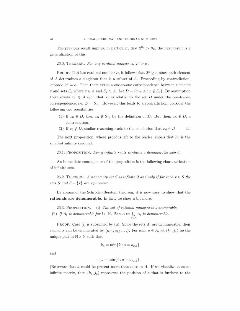
The previous result implies, in particular, that 2ℵ0 > ℵ0; the next result is a
generalization of this.
26.0. Theorem. For any cardinal number α, 2α > α.
Proof. If A has cardinal number α, it follows that 2α ≥ α since each element
of A determines a singleton that is a subset of A. Proceeding by contradiction,
suppose 2α = α. Then there exists a one-to-one correspondence between elements
x and sets Sx where x ∈ A and Sx ⊂ A. Let D = x ∈ A : x /∈ Sx. By assumption
there exists x0 ∈ A such that x0 is related to the set D under the one-to-one
correspondence, i.e. D = Sx0 . However, this leads to a contradiction; consider the
following two possibilities:
(1) If x0 ∈ D, then x0 /∈ Sx0by the definition of D. But then, x0 /∈ D, a
contradiction.
(2) If x0 /∈ D, similar reasoning leads to the conclusion that x0 ∈ D .
The next proposition, whose proof is left to the reader, shows that ℵ0 is the
smallest infinite cardinal.
26.1. Proposition. Every infinite set S contains a denumerable subset.
An immediate consequence of the proposition is the following characterization
of infinite sets.
26.2. Theorem. A nonempty set S is infinite if and only if for each x ∈ S the
sets S and S − x are equivalent
By means of the Schroder-Berstein theorem, it is now easy to show that the
rationals are denumerable. In fact, we show a bit more.
26.3. Proposition. (i) The set of rational numbers is denumerable,
(ii) If Ai is denumerable for i ∈ N, then A :=⋃i∈N
Ai is denumerable.
Proof. Case (i) is subsumed by (ii). Since the sets Ai are denumerable, their
elements can be enumerated by ai,1, ai,2, . . .. For each a ∈ A, let (ka, ja) be the
unique pair in N× N such that
ka = mink : a = ak,j
and
ja = minj : a = aka,j.
(Be aware that a could be present more than once in A. If we visualize A as an
infinite matrix, then (ka, ja) represents the position of a that is furthest to the
2.2. CARDINAL NUMBERS 27
“northwest” in the matrix.) Consequently, A is equivalent to a subset of N × N.
Further, observe that there is an injection of N× N into N given by
(i, j)→ 2i3j .
Indeed, if this were not an injection, we would have
2i−i′3j−j
′= 1
for some distinct positive integers i, i′, j, and j′, which is impossible. Thus, it
follows that A is equivalent to a subset of N and is therefore equivalent to a subset
of A1 because N ∼ A1. Since A1 ⊂ A we can now appeal to the Schroder-Bernstein
Theorem to arrive at the desired conclusion.
It is natural to ask whether the real numbers are also denumerable. This turns
out to be false, as the following two results indicate. It was G. Cantor who first
proved this fact.
27.1. Theorem. If I1 ⊃ I2 ⊃ I3 ⊃ . . . are closed intervals with the property
that length Ii → 0, then∞⋂i=1
Ii = x0
for some point x0 ∈ R.
Proof. Let Ii = [ai,bi] and choose xi ∈ Ii. Then xi is a Cauchy sequence
of real numbers since |xi − xj | ≤ max[lengthIi, lengthIj ]. Since R is complete
(Theorem 18.2), there exists x0 ∈ R such that
(27.1) limi→∞
xi = x0.
We claim that
(27.2) x0 ∈∞⋂i=1
Ii
for if not, there would be some positive integer i0 for which x0 /∈ Ii0 . Therefore,
since Ii0 is closed, there would be an η > 0 such that |x0 − y| > η for each y ∈ Ii0 .
Since the intervals are nested, it would follow that x0 /∈ Ii for all i ≥ i0 and thus
|x0 − xi| > η for all i ≥ i0. This would contradict (27.1) thus establishing (27.2).
We leave it to the reader to verify that x0 is the only point with this property.
27.2. Corollary. Every real number has a decimal representation relative to
any base.
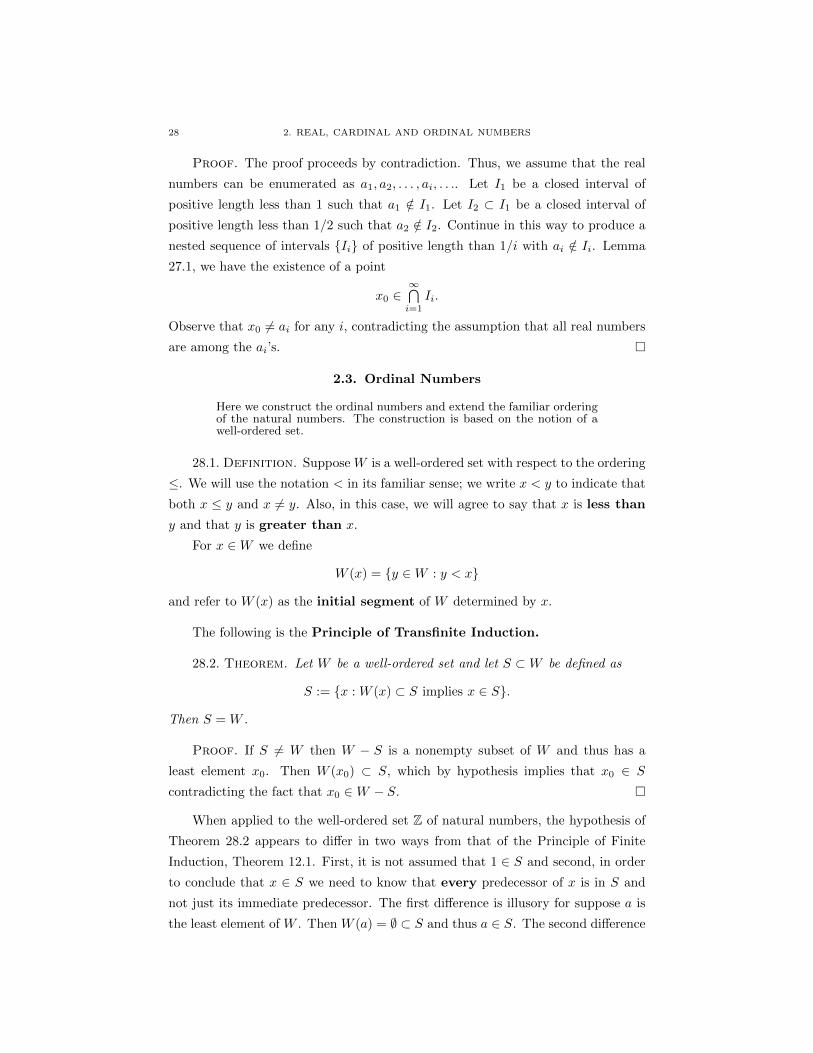
27.3. Theorem. The real numbers are uncountable.
28 2. REAL, CARDINAL AND ORDINAL NUMBERS
Proof. The proof proceeds by contradiction. Thus, we assume that the real
numbers can be enumerated as a1, a2, . . . , ai, . . .. Let I1 be a closed interval of
positive length less than 1 such that a1 /∈ I1. Let I2 ⊂ I1 be a closed interval of
positive length less than 1/2 such that a2 /∈ I2. Continue in this way to produce a
nested sequence of intervals Ii of positive length than 1/i with ai /∈ Ii. Lemma
27.1, we have the existence of a point
x0 ∈∞⋂i=1
Ii.
Observe that x0 6= ai for any i, contradicting the assumption that all real numbers
are among the ai’s.
2.3. Ordinal Numbers
Here we construct the ordinal numbers and extend the familiar orderingof the natural numbers. The construction is based on the notion of awell-ordered set.
28.1. Definition. Suppose W is a well-ordered set with respect to the ordering
≤. We will use the notation < in its familiar sense; we write x < y to indicate that
both x ≤ y and x 6= y. Also, in this case, we will agree to say that x is less than
y and that y is greater than x.
For x ∈W we define
W (x) = y ∈W : y < x
and refer to W (x) as the initial segment of W determined by x.
The following is the Principle of Transfinite Induction.
28.2. Theorem. Let W be a well-ordered set and let S ⊂W be defined as
S := x : W (x) ⊂ S implies x ∈ S.
Then S = W .
Proof. If S 6= W then W − S is a nonempty subset of W and thus has a
least element x0. Then W (x0) ⊂ S, which by hypothesis implies that x0 ∈ S
contradicting the fact that x0 ∈W − S.
When applied to the well-ordered set Z of natural numbers, the hypothesis of
Theorem 28.2 appears to differ in two ways from that of the Principle of Finite
Induction, Theorem 12.1. First, it is not assumed that 1 ∈ S and second, in order
to conclude that x ∈ S we need to know that every predecessor of x is in S and
not just its immediate predecessor. The first difference is illusory for suppose a is
the least element of W . Then W (a) = ∅ ⊂ S and thus a ∈ S. The second difference
2.3. ORDINAL NUMBERS 29
is more significant because, unlike the case of N, an element of an arbitrary well-
ordered set may not have an immediate predecessor.
29.0. Definition. A mapping ϕ from a well-ordered set V into a well-ordered
set W is order-preserving if ϕ(v1) ≤ ϕ(v2) whenever v1, v2 ∈ V and v1 ≤ v2. If, in
addition, ϕ is a bijection we will refer to it as an (order-preserving) isomorphism.
Note that, in this case, v1 < v2 implies ϕ(v1) < ϕ(v2); in other words, an order-
preserving isomorphism is strictly order-preserving.
Note: We have slightly abused the notation by using the same symbol ≤ to
indicate the ordering in both V and W above. But this should cause no confusion.
29.1. Lemma. If ϕ is an order-preserving injection of a well-ordered set W into
itself, then
w ≤ ϕ(w)
for each w ∈W .
Proof. Set
S = w ∈W : ϕ(w) < w.
If S is not empty, then it has a least element, say a. Thus ϕ(a) < a and consequently
ϕ(ϕ(a)) < ϕ(a) since ϕ is an order-preserving injection; moreover, ϕ(a) 6∈ S since
a is the least element of S. By the definition of S, this implies ϕ(a) ≤ ϕ(ϕ(a)),
which is a contradiction.
29.2. Corollary. If V and W are two well-ordered sets, then there is at most
one isomorphism of V onto W .
Proof. Suppose f and g are isomorphisms of V onto W . Then g−1 f is an
isomorphism of V onto itself and hence v ≤ g−1 f(v) for each v ∈ V . This implies
that g(v) ≤ f(v) for each v ∈ V . Since the same argument is valid with the roles
of f and g interchanged, we see that f = g.
29.3. Corollary. If W is a well-ordered set, then W is not isomorphic to an
initial segment of itself
Proof. Suppose a ∈ W and Wf−→ W (a) is an isomorphism. Since w ≤
f(w) for each w ∈ W , in particular we have a ≤ f(a). Hence f(a) 6∈ W (a), a
contradiction.
29.4. Corollary. No two distinct initial segments of a well ordered set W are
isomorphic.
30 2. REAL, CARDINAL AND ORDINAL NUMBERS
Proof. Since one of the initial segments must be an initial segment of the
other, the conclusion follows from the previous result.
30.1. Definition. We define an ordinal number as an equivalence class of
well-ordered sets with respect to order-preserving isomorphisms. If W is a well-
ordered set, we denote the corresponding ordinal number by ord(W ). We define a
linear ordering on the class of ordinal numbers as follows: if v = ord(V ) and w=
ord(W ), then v < w if and only if V is isomorphic to an initial segment of W . The
fact that this defines a linear ordering follows from the next result.
30.2. Theorem. If v and w are ordinal numbers, then precisely one of the
following holds:
(i) v = w
(ii) v < w
(iii) v > w
Proof. Let V and W be well-ordered sets representing v, w respectively and
let F denote the family of all order isomorphisms from an initial segment of V (or
V itself) onto either an initial segment of W (or W itself). Recall that a mapping
from a subset of V into W is a subset of V ×W . We may assume that V 6= ∅ 6= W .
If v and w are the least elements of V and W respectively, then (v, w) ∈ F and so
F is not empty. Ordering F by inclusion, we see that any linearly ordered subset S
of F has an upper bound; indeed the union of the subsets of V ×W corresponding
to the elements of S is easily seen to be an order isomorphism and thus an upper
bound for S. Therefore we may employ Zorn’s lemma to conclude that F has a
maximal element, say h. Since h ∈ F , it is an order isomorphism and h ⊂ V ×W .
If domainh and rangeh were initial segments say Vx and Wy of V and W , then
h∗ := h ∪ (x, y) would contradict the maximality of h unless domainh = V or
rangeh = W . If domainh = V , then either rangeh = W (i.e. v < w) or rangeh is
an initial segment of W , (i.e., v = w). If domainh 6= V , then domainh is an initial
segment of V and rangeh = W and the existence of h−1 in this case establishes
v > w.
30.3. Theorem. The class of ordinal numbers is well-ordered.
Proof. Let S be a nonempty set of ordinal numbers. Let α ∈ S and set
T = β ∈ S : β < α.
If T = ∅, then α is the least element of S. If T 6= ∅, let W be a well-ordered set
such that α= ord(W ). For each β ∈ T there is a well-ordered set Wβ such that β=
2.3. ORDINAL NUMBERS 31
ord(Wβ), and there is a unique xβ ∈ W such that Wβ is isomorphic to the initial
segment W (xβ) of W . The nonempty subset xβ : β ∈ T of W has a least element
xβ0. The element β0 ∈ T is the least element of T and thus the least element of
S.
31.1. Corollary. The cardinal numbers are comparable.
Proof. Suppose a is a cardinal number. Then, the set of all ordinals whose
cardinal number is a forms a well-ordered set that has a least element, call it α(a).
The ordinal α(a) is called the initial ordinal of a. Suppose b is another cardinal
number and let W (a) and W (b) be the well-ordered sets whose ordinal numbers
are α(a) and α(b), respectively. Either one of W (a) or W (b) is isomorphic to an
initial segment of the other if a and b are not of the same cardinality. Thus, one of
the sets W (a) and W (b) is equivalent to a subset of the other.
31.2. Corollary. Suppose α is an ordinal number. Then
α = ord(β : β is an ordinal number and β < α).
Proof. Let W be a well-ordered set such that α = ord(W ). Let β < α and
let W (β) be the initial segment of W whose ordinal number is β. It is easy to
verify that this establishes an isomorphism between the elements of W and the set
of ordinals less than α.
We may view the positive integers N as ordinal numbers in the following way.
Set
1 = ord(1),
2 = ord(1, 2),
3 = ord(1, 2, 3),
...
ω = ord(N).
We see that
(31.1) n < ω for each n ∈ N.
If β = ord(W ) < ω, then W must be isomorphic to an initial segment of N, i.e.,
β = n for some n ∈ N. Thus ω is the first ordinal number such that (31.1) holds
and is thus the first infinite ordinal.
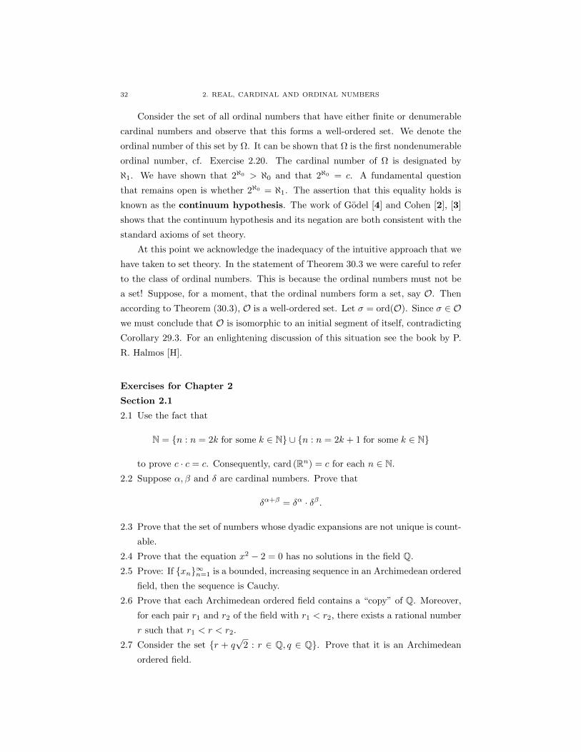
32 2. REAL, CARDINAL AND ORDINAL NUMBERS
Consider the set of all ordinal numbers that have either finite or denumerable
cardinal numbers and observe that this forms a well-ordered set. We denote the
ordinal number of this set by Ω. It can be shown that Ω is the first nondenumerable
ordinal number, cf. Exercise 2.20. The cardinal number of Ω is designated by
ℵ1. We have shown that 2ℵ0 > ℵ0 and that 2ℵ0 = c. A fundamental question
that remains open is whether 2ℵ0 = ℵ1. The assertion that this equality holds is
known as the continuum hypothesis. The work of Godel [4] and Cohen [2], [3]
shows that the continuum hypothesis and its negation are both consistent with the
standard axioms of set theory.
At this point we acknowledge the inadequacy of the intuitive approach that we
have taken to set theory. In the statement of Theorem 30.3 we were careful to refer
to the class of ordinal numbers. This is because the ordinal numbers must not be
a set! Suppose, for a moment, that the ordinal numbers form a set, say O. Then
according to Theorem (30.3), O is a well-ordered set. Let σ = ord(O). Since σ ∈ Owe must conclude that O is isomorphic to an initial segment of itself, contradicting
Corollary 29.3. For an enlightening discussion of this situation see the book by P.
R. Halmos [H].
Exercises for Chapter 2
Section 2.1
2.1 Use the fact that
N = n : n = 2k for some k ∈ N ∪ n : n = 2k + 1 for some k ∈ N
to prove c · c = c. Consequently, card (Rn) = c for each n ∈ N.
2.2 Suppose α, β and δ are cardinal numbers. Prove that
δα+β = δα · δβ .
2.3 Prove that the set of numbers whose dyadic expansions are not unique is count-
able.
2.4 Prove that the equation x2 − 2 = 0 has no solutions in the field Q.
2.5 Prove: If xn∞n=1 is a bounded, increasing sequence in an Archimedean ordered
field, then the sequence is Cauchy.
2.6 Prove that each Archimedean ordered field contains a “copy” of Q. Moreover,
for each pair r1 and r2 of the field with r1 < r2, there exists a rational number
r such that r1 < r < r2.
2.7 Consider the set r + q√
2 : r ∈ Q, q ∈ Q. Prove that it is an Archimedean
ordered field.
EXERCISES FOR CHAPTER 2 33
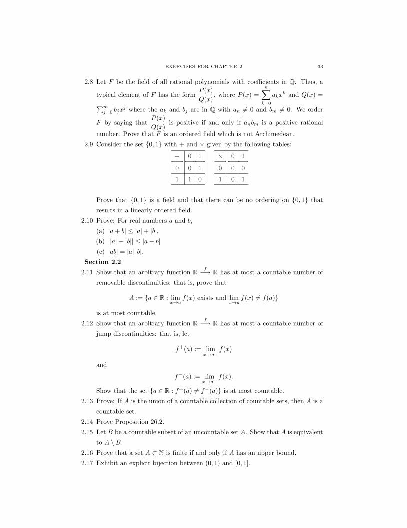
2.8 Let F be the field of all rational polynomials with coefficients in Q. Thus, a
typical element of F has the formP (x)
Q(x), where P (x) =
n∑k=0
akxk and Q(x) =∑m
j=0 bjxj where the ak and bj are in Q with an 6= 0 and bm 6= 0. We order
F by saying thatP (x)
Q(x)is positive if and only if anbm is a positive rational
number. Prove that F is an ordered field which is not Archimedean.
2.9 Consider the set 0, 1 with + and × given by the following tables:
+ 0 1
0 0 1
1 1 0
× 0 1
0 0 0
1 0 1
Prove that 0, 1 is a field and that there can be no ordering on 0, 1 that
2.11 Show that an arbitrary function R f−→ R has at most a countable number of
removable discontinuities: that is, prove that
A := a ∈ R : limx→a
f(x) exists and limx→a
f(x) 6= f(a)
is at most countable.
2.12 Show that an arbitrary function R f−→ R has at most a countable number of
jump discontinuities: that is, let
f+(a) := limx→a+
f(x)
and
f−(a) := limx→a−
f(x).
Show that the set a ∈ R : f+(a) 6= f−(a) is at most countable.
2.13 Prove: If A is the union of a countable collection of countable sets, then A is a
countable set.
2.14 Prove Proposition 26.2.
2.15 Let B be a countable subset of an uncountable set A. Show that A is equivalent
to A \B.
2.16 Prove that a set A ⊂ N is finite if and only if A has an upper bound.
2.17 Exhibit an explicit bijection between (0, 1) and [0, 1].
34 2. REAL, CARDINAL AND ORDINAL NUMBERS
2.18 If you are working in Zermelo-Fraenkel set theory without the Axiom of Choice,
can you choose an element from...
a finite set?
an infinite set?
each member of an infinite set of singletons (i.e., one-element sets)?
each member of an infinite set of pairs of shoes?
each member of an infinite set of pairs of socks?
each member of a finite set of sets if each of the members is infinite?
each member of an infinite set of sets if each of the members is infinite?
each member of a denumerable set of sets if each of the members is infinite?
each member of an infinite set of sets of rationals?
each member of a denumerable set of sets if each of the members is denumer-
able?
each member of an infinite set of sets if each of the members is finite?
each member of an infinite set of finite sets of reals?
each member of an infinite set of sets of reals?
each member of an infinite set of two-element sets whose members are sets of
reals?
Section 2.3
2.19 If E is a set of ordinal numbers, prove that that there is an ordinal number α
such that α > β for each β ∈ E.
2.20 Prove that Ω is the smallest nondenumerable ordinal.
2.21 Prove that the cardinality of all open sets in Rn is c.
2.22 Prove that the cardinality of all countable intersections of open sets in Rn is c.
2.23 Prove that the cardinality of all sequences of real numbers is c.
2.24 Prove that there are uncountably many subsets of an infinite set that are infi-
nite.
CHAPTER 3
Elements of Topology
3.1. Topological Spaces
The purpose of this short chapter is to provide enough point set topologyfor the development of the subsequent material in real analysis. An in-depth treatment is not intended. In this section, we begin with basicconcepts and properties of topological spaces.
Here, instead of the word “set,” the word “space” appears for the first time. Often
the word “space” is used to designate a set that has been endowed with a special
structure. For example a vector space is a set, such as Rn, that has been endowed
with an algebraic structure. Let us now turn to a short discussion of topological
spaces.
35.1. Definition. The pair (X, T ) is called a topological space where X is
a nonempty set and T is a family of subsets of X satisfying the following three
conditions:
(i) The empty set ∅ and the whole space X are elements of T ,
(ii) If S is an arbitrary subcollection of T , then⋃U : U ∈ S ∈ T ,
(iii) If S is any finite subcollection of T , then⋂U : U ∈ S ∈ T .
The collection T is called a topology for the space X and the elements of T are
called the open sets of X. An open set containing a point x ∈ X is called a
neighborhood of x. The interior of an arbitrary set A ⊂ X is the union of all
open sets contained in A and is denoted by Ao. Note that Ao is an open set and
that it is possible for some sets to have an empty interior. A set A ⊂ X is called
closed if X \A : = A is open. The closure of a set A ⊂ X, denoted by A, is
A = X ∩ x : U ∩A 6= ∅ for each open set U containing x
and the boundary of A is ∂A = A \Ao. Note that A ⊂ A.
35
36 3. ELEMENTS OF TOPOLOGY
These definitions are fundamental and will be used extensively throughout this
text.
36.0. Definition. A point x0 is called a limit point of a set A ⊂ X provided
A∩U contains a point of A different from x0 whenever U is an open set containing
x0. The definition does not require x0 to be an element of A. We will use the
notation A∗ to denote the set of limit points of A.
36.1. Examples. (i) If X is any set and T the family of all subsets of X,
then T is called the discrete topology. It is the largest topology (in the
sense of inclusion) that X can possess. In this topology, all subsets of X are
open.
(ii) The indiscrete is where T is taken as only the empty set ∅ and X itself; it
is obviously the smallest topology on X. In this topology, the only open sets
are X and ∅.(iii) Let X = Rn and let T consist of all sets U satisfying the following property:
for each point x ∈ U there exists a number r > 0 such that B(x, r) ⊂ U .
Here, B(x, r) denotes the ball or radius r centered at x; that is,
B(x, r) = y : |x− y| < r.
It is easy to verify that T is a topology. Note that B(x, r) itself is an open set.
This is true because if y ∈ B(x, r) and t = r − |y − x|, then an application of
the triangle inequality shows that B(y, t) ⊂ B(x, r). Of course, for n = 1, we
have that B(x, r) is an open interval in R.
(iv) Let X = [0, 1] ∪ (1, 2) and let T consist of 0 and 1 along with all open
sets (open relative to R) in (0, 1)∪ (1, 2). Then the open sets in this topology
contain, in particular, [0, 1] and [1, 2).
36.2. Definition. Suppose Y ⊂ X and T is a topology for X. Then it is easy
to see that the family S of sets of the form Y ∩U where U ranges over all elements
of T satisfies the conditions for a topology on Y . The topology formed in this way
is called the induced topology or equivalently, the relative topology on Y . The
space Y is said to inherit the topology from its parent space X.
36.3. Example. Let X = R2 and let T be the topology described in (iii)
above. Let Y = R2 ∩ x = (x1, x2) : x2 ≥ 0 ∪ x = (x1, x2) : x1 = 0. Thus, Y
is the upper half-space of R2 along with both the horizontal and vertical axes. All
intervals I of the form I = x = (x1, x2) : x1 = 0, a < x2 < b < 0, where a and
b are arbitrary negative real numbers, are open in the induced topology on Y , but
none of them is open in the topology on X. However, all intervals J of the form
3.1. TOPOLOGICAL SPACES 37
J = x = (x1, x2) : x1 = 0, a ≤ x2 ≤ b are closed both in the relative topology
and the topology on X.
37.1. Theorem. Let (X, T ) be a topological space. Then
(i) The union of an arbitrary collection of open sets is open.
(ii) The intersection of a finite number of open sets is open.
(iii) The union of a finite number of closed sets is closed.
(iv) The intersection of an arbitrary collection of closed sets is closed.
(v) A ∪B = A ∪B whenever A,B ⊂ X.
(vi) If Aα is an arbitrary collection of subsets of X, then⋃αAα ⊂
⋃αAα.
(vii) A ∩B ⊂ A ∩B whenever A,B ⊂ X.
(viii) A set A ⊂ X is closed if and only if A = A.
(ix) A = A ∪A∗
Proof. Parts (i) and (ii) constitute a restatement of the definition of a topo-
logical space. Parts (iii) and (iv) follow from (i) and (ii) and de Morgan’s laws,
2.2.
(v) Since A ⊂ A ∪B, we have A ⊂ A ∪B. Similarly, B ⊂ A ∪B, thus proving
A ∪B ⊃ A ∪ B. By contradiction, suppose the converse if not true. Then there
exists x ∈ A ∪B with x /∈ A ∪ B and therefore there exist open sets U and V
containing x such that U ∩ A = ∅ = V ∩ B. However, since U ∩ V is an open set
containing x, it follows that
∅ 6= (U ∩ V ) ∩ (A ∪B) ⊂ (U ∩A) ∪ (V ∩B) = ∅,
a contradiction.
(vi) This follows from the same reasoning used to establish the first part of (v).
(vii) This is immediate from definitions.
(viii) If A = A, then A is open (and thus A is closed) because x 6∈ A implies
that there exists an open set U containing x with U ∩ A = ∅; that is, U ⊂ A.
Conversely, if A is closed and x ∈ A, then x belongs to some open set U with
U ⊂ A. Thus, U ∩ A = ∅ and therefore x /∈ A. This proves A ⊂ (A)∼ or A ⊂ A.
But always A ⊂ A and hence, A = A.
(ix) is left as exercise 3.2.
37.2. Definition. Let (X, T ) be a topological space and xi∞i=1 a sequence
in X. The sequence is said to converge to x0 ∈ X if for each neighborhood U of
x0 there is a positive integer N such that xi ∈ U whenever i ≥ N .
38 3. ELEMENTS OF TOPOLOGY
It is important to observe that the structure of a topological space is so general
that a sequence could possibly have more than one limit. For example, every
sequence in the space with the indiscrete topology (Example 36.1 (ii)) converges
to every point in X. This cannot happen if an additional restriction is placed
on the topological structure, as in the following definition. (Also note that the
only sequences that converge in the discrete topology are those that are eventually
constant.)
38.1. Definition. A topological space X is said to be a Hausdorff space if
for each pair of distinct points x1, x2 ∈ X there exist disjoint open sets U1 and U2
containing x1 and x2 respectively. That is, two distinct points can be separated
by disjoint open sets.
38.2. Definition. Suppose (X, T ) and (Y,S) are topological spaces. A func-
tion f : X → Y is said to be continuous at x0 ∈ X if for each neighborhood V
containing f(x0) there is a neighborhood U of x0 such that f(U) ⊂ V . The function
f is said to be continuous on X if it is continuous at each point x ∈ X.
The proof of the next result is given as Exercise 3.4.
38.3. Theorem. Let (X, T ) and (Y,S) be topological spaces. Then for a func-
tion f : X → Y , the following statements are equivalent:
(i) f is continuous.
(ii) f−1(V ) is open in X for each open set V in Y .
(iii) f−1(K) is closed in X for each closed set K in Y .
38.4. Definition. A collection of open sets, F , in a topological space X is said
to be an open cover of a set A ⊂ X if
A ⊂⋃U∈F
U.
The family F is said to admit a subcover, G, of A if G ⊂ F and G is a cover of
A. A subset K ⊂ X is called compact if each open cover of K possesses a finite
subcover of K. A space X is said to be locally compact if each point of X is
contained in some open set whose closure is compact.
It is easy to give illustrations of sets that are not compact. For example, it is
readily seen that the set A = (0, 1] in R is not compact since the collection of open
intervals of the form (1/i, 2), i = 1, 2, . . ., provides an open cover of A admits no
finite subcover. On the other hand, it is true that [0, 1] is compact, but the proof
is not obvious. The reason for this is that the definition of compactness is usually
3.1. TOPOLOGICAL SPACES 39
not easy to employ directly. Later, in the context of metric spaces (Section 3.3),
we will find other ways of dealing with compactness.
The following two propositions reveal some basic connections between closed
and compact subsets.
39.1. Proposition. Let (X, T ) be a topological space. If A and K are respec-
tively closed and compact subsets of X with A ⊂ K, then A is compact.
Proof. If F is an open cover of A, then the elements of F along with X \ Aform an open cover of K. This open cover has a finite subcover, G, of K since K is
compact. The set X \A may possibly be an element of G. If X \A is not a member
of G, then G is a finite subcover of A; if X \A is a member of G, then G with X \Aomitted is a finite subcover of A.
39.2. Proposition. A compact subset of a Hausdorff space (X, T ) is closed.
Proof. We will show that X \K is open where K ⊂ X is compact. Choose a
fixed x0 ∈ X \K and for each y ∈ K, let Vy and Uy denote disjoint neighborhoods
of y and x0 respectively. The family
F = Vy : y ∈ K
forms an open cover of K. Hence, F possesses a finite subcover, say Vyi : i =
1, 2, . . . , N. Since Vyi∩Uyi = ∅, i = 1, 2, . . . , N , it follows thatN∩i=1
Uyi ∩N∪i=1
Vyi = ∅.
Since K ⊂N∪i=1
Vyi it follows thatN∩i=1
Vyi is an open set containing x0 that does not
intersect K. Thus, X \K is an open set, as desired.
The characteristic property of a Hausdorff space is that two distinct points can
be separated by disjoint open sets. The next result shows that a stronger property
holds, namely, that a compact set and a point not in this compact set can be
separated by disjoint open sets.
39.3. Proposition. Suppose K is a compact subset of a Hausdorff space X
space and assume x0 6∈ K. Then there exist disjoint open sets U and V containing
x0 and K respectively.
Proof. This follows immediately from the preceding proof by taking
U =N⋂i=1
Uyi and V =N⋃i=1
Vyi .
39.4. Definition. A family Eα : α ∈ I of subsets of a set X is said to have
the finite intersection property if for each finite subset F ⊂ I⋂α∈F
Eα 6= ∅.
40 3. ELEMENTS OF TOPOLOGY
39.5. Lemma. A topological space X is compact if and only if every family of
closed subsets of X having the finite intersection property has a nonempty intersec-
tion.
Proof. First assume that X is compact and let Cα be a family of closed sets
with the finite intersection property. Then Uα := X \Cα is a family, F , of open
sets. If⋂αCα were empty, then F would form an open covering of X and therefore
the compactness of X would imply that F has a finite subcover. This would imply
that Cα has a finite subfamily with an empty intersection, contradicting the fact
that Cα has the finite intersection property.
For the converse, let Uα be an open covering of X and let Cα := X \Uα.If Uα had no finite subcover of X, then Cα would have the finite intersection
property, and therefore,⋂αCα would be nonempty, thus contradicting the assump-
tion that Uα is a covering of X.
40.1. Remark. An equivalent way of stating the previous result is as follows:
A topological space X is compact if and only if every family of closed subsets of X
whose intersection is empty has a finite subfamily whose intersection is also empty.
40.2. Theorem. Suppose K ⊂ U are respectively compact and open sets in a
locally compact Hausdorff space X. Then there is an open set V whose closure is
compact such that
K ⊂ V ⊂ V ⊂ U.
Proof. Since each point of K is contained in an open set whose closure is
compact, and since K can be covered by finitely many such open sets, it follows
that the union of these open sets, call it G, is an open set containing K with
compact closure. Thus, if U = X, the proof is compete.
Now consider the case U 6= X. Proposition 39.3 states that for each x ∈ U
there is an open set Vx such that K ⊂ Vx and x 6∈ V x. Let F be the family of
compact sets defined by
F := U ∩G ∩ V x : x ∈ U.
and observe that the intersection of all sets in F is empty, for otherwise, we would
be faced with impossibility of some x0 ∈ U ∩G that also belongs to V x0 . Lemma
39.5 (or Remark 40.1) implies there is some finite subfamily of F that has an empty
intersection. That is, there exist points x1, x2, . . . , xk ∈ U such that
U ∩G ∩ V x1∩ · · · ∩ V xk = ∅.
3.2. BASES FOR A TOPOLOGY 41
The set
V = G ∩ Vx1 ∩ · · · ∩ Vxksatisfies the conclusion of our theorem since
K ⊂ V ⊂ V ⊂ G ∩ V x1 ∩ · · · ∩ V xk ⊂ U.
3.2. Bases for a Topology
Often a topology is described in terms of a primitive family of sets,called a basis. We will give a brief description of this concept.
41.1. Definition. A collection B of open sets in a topological space (X, T )
is called a basis for the topology T if and only if B is a subfamily of T with the
property that for each U ∈ T and each x ∈ U , there exists B ∈ B such that
x ∈ B ⊂ U . A collection B of open sets containing a point x is said to be a basis at
x if for each open set U containing x there is a B ∈ B such that x ∈ B ⊂ U . Observe
that a collection B forms a basis for a topology if and only if it contains a basis at
each point x ∈ X. For example, the collection of all sets B(x, r), r > 0, x ∈ Rn,
provides a basis for the topology on Rn as described in (iii) of Example 36.1.
The following is a useful tool for generating a topology on a space X.
41.2. Proposition. Let X be an arbitrary space. A collection B of subsets of
X is a basis for some topology on X if and only if each x ∈ X is contained in some
B ∈ B and if x ∈ B1 ∩B2, then there exists B3 ∈ B such that x ∈ B3 ⊂ B1 ∩B2.
Proof. It is easy to verify that the conditions specified in the Proposition are
necessary. To show that they are sufficient, let T be the collection of sets U with
the property that for each x ∈ U , there exists B ∈ B such that x ∈ B ⊂ U . It is
easy to verify that T is closed under arbitrary unions. To show that it is closed
under finite intersections, it is sufficient to consider the case of two sets. Thus,
suppose x ∈ U1 ∩ U2, where U1 and U2 are elements of T . There exist B1, B2 ∈ Bsuch that x ∈ B1 ⊂ U1 and x ∈ B2 ⊂ U2. We are given that there is B3 ∈ B such
that x ∈ B3 ⊂ B1 ∩B2, thus showing that U1 ∩ U2 ∈ T .
41.3. Definition. A topological space (X, T ) is said to satisfy the first axiom
of countability if each point x ∈ X has a countable basis Bx at x. It is said to
satisfy the second axiom of countability if there is a countable basis B.
The second axiom of countability obviously implies the first axiom of count-
ability. The usual topology on Rn, for example, satisfies the second axiom of
countability.
42 3. ELEMENTS OF TOPOLOGY
41.4. Definition. A family S of subsets of a topological space (X, T ) is called
a subbase for the topology T if the family consisting of all finite intersections of
members of S forms a base for the topology T .
In view of Proposition 41.2, every nonempty family of subsets of X is the sub-
base for some topology on X. This leads to the concept of the product topology.
42.1. Definition. Given an index set A, consider the Cartesian product∏α∈AXα where each (Xα, Tα) is a topological space. For each β ∈ A there is a
natural projection
Pβ :∏α∈A
Xα → Xβ
defined by Pβ(x) = xβ where xβ is the β th coordinate of x, (See (5.1) and its
following remarks.) Consider the collection S of subsets of∏α∈AXα given by
P−1α (Vα)
where Vα ∈ Tα and α ∈ A. The topology formed by the subbase S is called the
product topology on∏α∈AXα. In this topology, the projection maps Pβ are
continuous.
It is easily seen that a function f from a topological space (Y, T ) into a product
space∏α∈AXα is continuous if and only if (Pα f) is continuous for each α ∈ A.
Moreover, a sequence xi∞i=1 in a product space∏α∈AXα converges to a point x0
of the product space if and only if the sequence Pα(xi)∞i=1 converges to Pα(x0)
for each α ∈ A. See Exercises 3.8 and 3.9.
3.3. Metric Spaces
Metric spaces are used extensively throughout analysis. The main pur-pose of this section is to introduce basic definitions.
We already have mentioned two structures placed on sets that deserve the
designation space, namely, vector space and topological space. We now come to
our third structure, that of a metric space.
42.2. Definition. A metric space is an arbitrary set X endowed with a metric
ρ : X ×X → [0,∞) that satisfies the following properties for all x, y and z in X:
(i) ρ(x, y) = 0 if and only if x = y,
(ii) ρ(x, y) = ρ(y, x),
(iii) ρ(x, y) ≤ ρ(x, z) + ρ(z, y).
3.3. METRIC SPACES 43
We will write (X, ρ) to denote the metric space X endowed with a metric ρ. Often
the metric ρ is called the distance function and a reasonable name for property (iii)
is the triangle inequality. If Y ⊂ X, then the metric space (Y, ρ (Y × Y )) is
called the subspace induced by (X, ρ).
The following are easily seen to be metric spaces.
43.1. Example.
(i) Let X = Rn and with x = (x1, . . . , xn), y = (y1, . . . , yn) ∈ Rn, define
ρ(x, y) =
(n∑i=1
|xi − yi|2)1/2
.
(ii) Let X = Rn and with x = (x1, . . . , xn), y = (y1, . . . , yn) ∈ Rn, define
ρ(x, y) = max|xi − yi| : i = 1, 2, . . . , n.
(iii) The discrete metric on and arbitrary set X is defined as follows: for x, y ∈X,
ρ(x, y) =
1 if x 6= y
0 if x = y .
(iv) Let X denote the space of all continuous functions defined on [0, 1] and for
f, g ∈ C(X), let
ρ(f, g) =
∫ 1
0
|f(t)− g(t)| dt.
(v) Let X denote the space of all continuous functions defined on [0, 1] and for
f, g ∈ C(X), let
ρ(f, g) = max|f(x)− g(x)| : x ∈ [0, 1]
43.2. Definition. If X is a metric space with metric ρ, the open ball centered
at x ∈ X with radius r > 0 is defined as
B(x, r) = X ∩ y : ρ(x, y) < r.
The closed ball is defined as
B(x, r) := X ∩ y : ρ(x, y) ≤ r.
In view of the triangle inequality, the family S = B(x, r) : x ∈ X, r > 0 forms a
basis for a topology T on X called the topology induced by ρ. The two metrics
in Rn defined in Examples 43.1, (i) and (ii) induce the same topology on Rn. Two
metrics on a set X are said to be topologically equivalent if they induce the
same topology on X.
44 3. ELEMENTS OF TOPOLOGY
43.3. Definition. Using the notion of convergence given in Definition 37.2,
p.37, the reader can easily verify that the convergence of a sequence xi∞i=1 in a
metric space (X, ρ) becomes the following:
limi→∞
xi = x0
if and only if for each positive number ε there is a positive integer N such that
ρ(xi, x0) < ε whenever i ≥ N.
We often write xi → x0 for limi→∞ xi = x0.
The notion of a fundamental or a Cauchy sequence is not a topological one
and requires a separate definition:
44.1. Definition. A sequence xi∞i=1 is called Cauchy if for every ε > 0,
there exists a positive integer N such that ρ(xi, xj) < ε whenever i, j ≥ N . The
notation for this is
limi,j→∞
ρ(xi, xj) = 0.
Recall the definition of continuity given in Definition 38.2. In a metric space,
it is convenient to have the following characterization whose proof is left as an
exercise.
44.2. Theorem. If (X, ρ) and (Y, σ) are metric spaces, then a mapping
f : X → Y is continuous at x ∈ X if for each ε > 0, there exists δ > 0 such that
σ[f(x), f(y)] < ε whenever ρ(x, y) < δ.
44.3. Definition. If X and Y are topological spaces and if f : X → Y is a
bijection with the property that both f and f−1 are continuous, then f is called
a homeomorphism and the spaces X and Y are said to be homeomorphic.
A substantial part of topology is devoted to the investigation of those properties
that remain unchanged under the action of a homeomorphism. For example, in
view of Exercise 3.21, it follows that if U ⊂ X is open, then so is f(U) whenever
f : X → Y is a homeomorphism; that is, the property of being open is a topological
invariant. Consequently, so is closedness. But of course, not all properties are
topological invariants. For example, the distance between two points might be
changed under a homeomorphism. A mapping that preserves distances, that is,
one for which
σ[f(x), f(y)] = ρ(x, y)
for all x, y ∈ X is called an isometry. In particular, it is a homeomorphism, The
spaces X and Y are called isometric if there exists a surjection f : X → Y that
3.4. MEAGER SETS IN TOPOLOGY 45
is an isometry. In the context of metric space topology, isometric spaces can be
regarded as being identical.
It is easy to verify that a convergent sequence in a metric space is Cauchy, but
the converse need not be true. For example, the metric space, Q, consisting of the
rational numbers endowed with the usual metric on R, possesses Cauchy sequences
that do not converge to elements in Q. If a metric space has the property that
every Cauchy sequence converges (to an element of the space), the space is said
to be complete. Thus, the metric space of rational numbers is not complete,
whereas the real numbers are complete. However, we can apply the technique that
was employed in the construction of the real numbers (see Section 2.1, p.11) to
complete an arbitrary metric space. A precise statement of this is incorporated in
the following theorem, whose proof is left as Exercise 3.30.
45.1. Theorem. If (X, ρ) is a metric space, there exists a complete metric
space (X∗, ρ∗) in which X is isometrically embedded as a dense subset.
In the statement, the notion of a dense set is used. This notion is a topological
one. In a topological space (X, T ), a subset A of X is said to be a dense subset of
X if X = A.
3.4. Meager Sets in Topology
Throughout this book, we will encounter several ways of describing the“size” of a set. In Chapter 2 the size of a set was described in terms ofits cardinality. Later, we will discuss other methods. The notion of anowhere dense set and its related concept, that of a set being of the firstcategory, are ways of saying that a set is “meager” in the topologicalsense. In this section we shall prove one of the main results involv-ing these concepts, the Baire Category Theorem, which asserts that acomplete metric space is not meager.
Recall Definition 42.2 in which a subset S of a metric space (X, ρ) is endowed
with the induced topology. The metric placed on S is obtained by restricting the
metric ρ to S × S. Thus, the distance between any two points x, y ∈ S is defined
as ρ(x, y), which is the distance between x, y as points of X.
As a result of the definition, a subset U ⊂ S is open in S if for each x ∈ U ,
there exists r > 0 such that if y ∈ S and ρ(x, y) < r, then y ∈ U . In other words,
B(x, r)∩S ⊂ U where B(x, r) is taken as the ball in X. Thus, it is easy to see that
U is open in S if and only if there exists an open set V in X such that U = V ∩ S.
Consequently, a set F ⊂ S is closed relative to S if and only if F = C ∩ S for some
closed set C in S. Moreover, the closure of a set E relative to S is E ∩ S, where E
denotes the closure of E in X. This is true because if a point x is in the closure of
E in X, then it is a point in the closure of E in S if it belongs to S.
46 3. ELEMENTS OF TOPOLOGY
45.2. Definitions. A subset E of a metric space X is said to be dense in an
open set U if E ⊃ U . Also, a set E is defined to be nowhere dense if it is not
dense in any open subset U of X. Alternatively, we could say that E is nowhere
dense if E does not contain any open set. For example, the integers comprise a
nowhere dense set in R, whereas the set Q∩ [0, 1] is not nowhere dense in R. A set
E is said to be of first category in X if it is the union of a countable collection
of nowhere dense sets. A set that is not of the first category is said to be of the
second category in X .
We now proceed to investigate a fundamental result related to these concepts.
46.1. Theorem (Baire Category Theorem). A complete metric space X is not
the union of a countable collection of nowhere dense sets. That is, a complete
metric space is of the second category.
Before going on, it is important to examine the statement of the theorem in
various contexts. For example, let X be the integers endowed with the metric
induced from R. Thus, X is a complete metric space and therefore, by the Baire
Category Theorem, it is of the second category. At first, this may seem counter
intuitive, since X is the union of a countable collection of points. But remember
that a point in this space is an open set, and therefore is not nowhere dense.
However, if X is viewed as a subset of R and not as a space in itself, then indeed,
X is the union of a countable number of nowhere dense sets.
Proof. Assume by contradiction, that X is of the first category. Then there
exists a countable collection of nowhere dense sets Ei such that
X =∞⋃i=1
Ei.
Let B(x1, r1) be an open ball with radius r1 < 1. Since E1 is not dense in any open
set, it follows that B(x1, r1) \ E1 6= ∅. This is a nonempty open set, and therefore
there exists a ball B(x2, r2) ⊂ B(x1, r1)\E1 with r2 <12r1. In fact, by also choosing
r2 smaller than r1 − ρ(x1, x2), we may assume that B(x2, r2) ⊂ B(x1, r1) \ E1.
Similarly, since E2 is not dense in any open set, we have that B(x2, r2) \ E2 is a
nonempty open set. As before, we can find a closed ball with center x3 and radius
r3 <12r2 <
122 r1
B(x3, r3) ⊂ B(x2, r2) \ E2
⊂(B(x1, r1) \ E1
)\ E2
= B(x1, r1) \2⋃j=1
Ej .
3.4. MEAGER SETS IN TOPOLOGY 47
Proceeding inductively, we obtain a nested sequence B(x1, r1) ⊃ B(x1, r1) ⊃B(x2, r2) ⊃ B(x2, r2) . . . with ri <
12i r1 → 0 such that
(46.1) B(xi+1, ri+1) ⊂ B(x1, r1) \i⋃
j=1
Ej
for each i. Now, for i, j > N , we have xi, xj ∈ B(xN , rN ) and therefore ρ(xi, xj) ≤2rN . Thus, the sequence xi is Cauchy in X. Since X is assumed to be complete,
it follows that xi → x for some x ∈ X. For each positive integer N, xi ∈ B(xN , rN )
for i ≥ N . Hence, x ∈ B(xN , rN ) for each positive integer N . For each positive
integer i it follows from (46.1) that
x ∈ B(xi+1, ri+1) ⊂ B(x1, r1) \i⋃
j=1
Ej .
In particular, for each i ∈ N
x 6∈i⋃
j=1
Ej
and therefore
x 6∈∞⋃j=1
Ej = X
a contradiction.
47.1. Definition. A function f : X → Y where (X, ρ) and (Y, σ) are metric
spaces is said to bounded if there exists 0 < M <∞ such that σ(f(x), f(y)) ≤Mfor all x, y ∈ X. A family F of functions f : X → Y is called uniformly bounded
if σ(f(x), f(y)) ≤M for all x, y ∈ X and for all f ∈ F .
An immediate consequence of the Baire Category Theorem is the following re-
sult, which is known as the uniform boundedness principle. We will encounter
this result again in the framework of functional analysis, Theorem 283.1. It states
that if the upper envelope of a family of continuous functions on a complete met-
ric space is finite everywhere, then the upper envelope is bounded above by some
constant on some nonempty open subset. In other words, the family is uniformly
bounded on some open set. Of course, there is no estimate of how large the open
set is, but in some applications just the knowledge that such an open set exists, no
matter how small, is of great importance.
47.2. Theorem. Let F be a family of real-valued continuous functions defined
on a complete metric space X and suppose
(47.1) f∗(x) : = supf∈F|f(x)| <∞
for each x ∈ X. That is, for each x ∈ X, there is a constant Mx such that
f(x) ≤Mx for all f ∈ F .
48 3. ELEMENTS OF TOPOLOGY
Then there exist a nonempty open set U ⊂ X and a constant M such that |f(x)| ≤M for all x ∈ U and all f ∈ F .
48.1. Remark. Condition (47.1) states that the family F is bounded at each
point x ∈ X; that is, the family is pointwise bounded by Mx. In applications, a
difficulty arises from the possibility that supx∈XMx =∞. The main thrust of the
theorem is that there exist M > 0 and an open set U such that supx∈U Mx ≤M .
Proof. For each positive integer i, let
Ei,f = x : |f(x)| ≤ i, Ei =⋂f∈F
Ei,f .
Note that Ei,f is closed and therefore so is Ei since f is continuous. From the
hypothesis, it follows that
X =∞⋃i=1
Ei.
Since X is a complete metric space, the Baire Category Theorem implies that there
is some set, say EM , that is not nowhere dense. Because EM is closed, it must
contain an open set U . Now for each x ∈ U , we have |f(x)| ≤ M for all f ∈ F ,
which is the desired conclusion.
48.2. Example. Here is a simple example which illustrates this result. Define
a sequence of functions fk : [0, 1]→ R by
fk(x) =
k2x, 0 ≤ x ≤ 1/k
−k2x+ 2k, 1/k ≤ x ≤ 2/k
0, 2/k ≤ x ≤ 1
Thus, fk(x) ≤ k on [0, 1] and f∗(x) ≤ k on [1/k, 1] and so f∗(x) < ∞ for all
0 ≤ x ≤ 1. The sequence fk is not uniformly bounded on [0, 1], but it is uniformly
bounded on some open set U ⊂ [0, 1]. Indeed, in this example, the open set U can
be taken as any interval (a, b) where 0 < a < b < 1 because the sequence fkisbounded by 1/k on (2/k, 1).
3.5. Compactness in Metric Spaces
In topology there are various notions related to compactness includ-ing sequential compactness and the Bolzano-Weierstrass Property. Themain objective of this section is to show that these concepts are equiv-alent in a metric space.
The concept of completeness in a metric space is very useful, but is limited to
only those sequences that are Cauchy. A stronger notion called sequential compact-
ness allows consideration of sequences that are not Cauchy. This notion is more
3.5. COMPACTNESS IN METRIC SPACES 49
general in the sense that it is topological, whereas completeness is meaningful only
in the setting of a metric space.
There is an abundant supply of sets that are not compact. For example, the
set A : = (0, 1] in R is not compact since the collection of open intervals of the form
(1/i, 2], i = 1, 2, . . ., provides an open cover of A that admits no finite subcover. On
the other hand, while it is true that [0, 1] is compact, the proof is not obvious. The
reason for this is that the definition of compactness usually is not easy to employ
directly. It is best to first determine how it intertwines with other related concepts.
49.1. Definition. Definition If (X, ρ) is a metric space, a set A ⊂ X is called
totally bounded if, for every ε > 0, A can be covered by finitely many balls of
radius ε. A set A is bounded if there is a positive number M such that ρ(x, y) ≤Mfor all x, y ∈ A. While it is true that a totally bounded set is bounded (Exercise
3.32), the converse is easily seen to be false; consider (iii) of Example 43.1.
49.2. Definition. A set A ⊂ X is said to be sequentially compact if every
sequence in A has a subsequence that converges to a point in A. Also, A is said to
have the Bolzano-Weierstrass property if every infinite subset of A has a limit
point that belongs to A.
49.3. Theorem. If A is a subset of a metric space (X, ρ), the following are
equivalent:
(i) A is compact.
(ii) A is sequentially compact.
(iii) A is complete and totally bounded.
(iv) A has the Bolzano-Weierstrass property.
Proof. Beginning with (i), we shall prove that each statement implies its
successor.
(i) implies (ii): Let xi be a sequence in A; that is, there is a function f defined
on the positive integers such that f(i) = xi for i = 1, 2, . . .. Let E denote the range
of f . If E has only finitely many elements, then some member of the sequence
must be repeated an infinite number of times thus showing that the sequence has
a convergent subsequence.
Assuming now that E is infinite we proceed by contradiction and thus sup-
pose that xi had no convergent subsequence. Then each element of E would
be isolated. That is, with each x ∈ E there exists r = rx > 0 such that
B(x, rx) ∩ E = x. This would imply that E has no limit points; thus, Theorem
37.1 (viii) and (ix), (p. 37), would imply that E is closed and therefore compact
by Proposition 39.1. However, this would lead to a contradiction since the family
50 3. ELEMENTS OF TOPOLOGY
B(x, rx) : x ∈ E is an open cover of E that possesses no finite subcover; this is
impossible since E consists of infinitely many points.
(ii) implies (iii): The denial of (iii) leads to two possibilities: Either A is not
complete or it is not totally bounded. If A were not complete, there would exist a
fundamental sequence xi in A that does not converge to any point in A. Hence,
no subsequence converges for otherwise the whole sequence would converge, thus
contradicting the sequential compactness of A.
On the other hand, suppose A is not totally bounded; then there exists ε > 0
such that A cannot be covered by finitely many balls of radius ε. In particular, we
conclude that A has infinitely many elements. Now inductively choose a sequence
xi in A as follows: select x1 ∈ A. Then, since A \ B(x1, ε) 6= ∅ we can choose
it is sufficient to show that Q is totally bounded. For this purpose, choose ε > 0
and let k be an integer such that k >√na/ε. Then Q can be expressed as the
union of kn congruent subcubes by dividing the interval [−a, a] into k equal pieces.
The side length of each of these subcubes is 2a/k and hence the diameter of each
52 3. ELEMENTS OF TOPOLOGY
cube is 2√na/k < 2ε. Therefore, each cube is contained in a ball of radius ε about
its center.
3.6. Compactness of Product Spaces
In this section we prove Tychonoff’s Theorem which states that theproduct of an arbitrary number of compact topological spaces is com-pact. This is one of the most important theorems in general topology,in particular for its applications to functional analysis.
Let Xα : α ∈ A be a family of topological spaces and set X =∏α∈AXα.
Let Pα : X → Xα denote the projection of X onto Xα for each α. Recall that the
family of subsets of X of the form P−1α (U) where U is an open subset of Xα and
α ∈ A is a subbase for the product topology on X.
The proof of Tychonoff’s theorem will utilize the finite intersection property
introduced in Definition 39.4 and Lemma 39.5.
In the following proof, we utilize the Hausdorff Maximal Principle, see p. 7.
52.1. Lemma. Let A be a family of subsets of a set Y having the finite inter-
section property and suppose A is maximal with respect to the finite intersection
property, i.e., no family of subsets of Y that properly contains A has the finite
intersection property. Then
(i) A contains all finite intersections of members of A.
(ii) If S ⊂ Y and S ∩A 6= ∅ for each A ∈ A, then S ∈ A.
Proof. To prove (i) let B denote the family of all finite intersections of mem-
bers of A. Then A ⊂ B and B has the finite intersection property. Thus by the
maximality of A, it is clear that A = B.
To prove (ii), suppose S ∩A 6= ∅ for each A ∈ A. Set C = A∪S. Then, since
C has the finite intersection property, the maximality of A implies that C = A.
We can now prove Tychonoff’s theorem.
52.2. Theorem (Tychonoff’s Product Theorem). If Xα : α ∈ A is a family
of compact topological spaces and X =∏α∈AXα with the product topology, then X
is compact.
Proof. Suppose C is a family of closed subsets of X having the finite inter-
section property and let E denote the collection of all families of subsets of X such
that each family contains C and has the finite intersection property. Then E satisfies
the conditions of the Hausdorff Maximal Principle, and hence there is a maximal
element B of E in the sense that B is not a subset of any other member of E .
3.7. THE SPACE OF CONTINUOUS FUNCTIONS 53
For each α the family Pα(B) : B ∈ B of subsets of Xα has the finite inter-
section property. Since Xα is compact, there is a point xα ∈ Xα such that
xα ∈⋂B∈B
Pα(B).
For any α ∈ A, let Uα be an open subset of Xα containing xα. Then
B⋂P−1α (Uα) 6= ∅
for each B ∈ B. In view of Lemma 52.1 (ii) we see that P−1α (Uα) ∈ B. Thus by
Lemma 52.1 (i), any finite intersection of sets of this form is a member of B. It
follows that any open subset of X containing x has a nonempty intersection with
each member of B. Since C ⊂ B and each member of C is closed, it follows that
x ∈ C for each C ∈ C.
3.7. The Space of Continuous Functions
In this section we investigate an important metric space, C(X), thespace of continuous functions on a metric space X. It is shown that thisspace is complete. More importantly, necessary and sufficient conditionsfor the compactness of subsets of C(X) are given.
Recall the discussion of continuity given in Theorems 38.3 and 44.2. Our dis-
cussion will be carried out in the context of functions f : X → Y where (X, ρ) and
(Y, σ) are metric spaces. Continuity of f at x0 requires that points near x0 are
mapped into points near f(x0). We introduce the concept of “oscillation” to assist
in making this idea precise.
53.1. Definition. If f : X → Y is an arbitrary mapping, then the oscillation
Thus, the oscillation of f on a ball B(x0, r) is nothing more than the diam-
eter of the set f(B(x0, r)) in Y . The diameter of an arbitrary set E is defined
as supσ(x, y) : x, y ∈ E. It may possibly assume the value +∞. Note that
osc [f,B(x0, r)] is a nondecreasing function of r for each point x0.
We leave it to the reader to supply the proof of the following assertion.
53.2. Proposition. A function f : X → Y is continuous at x0 ∈ X if and only
if
limr→0
osc [f,B(x0, r)] = 0.
54 3. ELEMENTS OF TOPOLOGY
The concept of oscillation is useful in providing information concerning the set
on which an arbitrary function is continuous.
For this we need the following definitions
54.1. Definition. A subset E of a topological space is called a Gδ set if E
can be written as the countable intersection of open sets, and it is an Fσ set if it
can be written as the countable union of closed sets.
54.2. Theorem. Let f : X → Y be an arbitrary function. Then the set of
points at which f is continuous is a Gδ set.
Proof. For each integer i, let
Gi = X ∩ x : infr>0
osc [f,B(x, r)] < 1/i.
From the Proposition above, we know that f is continuous at x if and only if
limr→0 osc [f,B(x, r)] = 0. Therefore, the set of points at which f is continuous is
given by
A =∞⋂i=1
Gi.
To complete the proof we need only show that each Gi is open. For this, observe
that if x ∈ Gi, then there exists r > 0 such that osc [f,B(x, r)] < 1/i. Now for each
y ∈ B(x, r), there exists t > 0 such that B(y, t) ⊂ B(x, r) and consequently,
osc [f,B(y, t)] ≤ osc [f,B(x, r)] < 1/i.
This implies that each point y of B(x, r) is an element of Gi. That is, B(x, r) ⊂ Giand since x is an arbitrary point of Gi, it follows that Gi is open.
54.3. Theorem. Let f be an arbitrary function defined on [0, 1] and let E :=
x ∈ [0, 1] : f is continuous at x. Then E cannot be the set of rational numbers in
[0, 1].
Proof. It suffices to show that the rationals in [0, 1] do not constitute a Gδ
set. If this were false, the irrationals in [0, 1] would be an Fσ set and thus would be
the union of a countable number of closed sets, each having an empty interior. Since
the rationals are a countable union of closed sets (singletons, with no interiors), it
would follow that [0, 1] is also of the first category, contrary to the Baire Category
Theorem. Thus, the rationals cannot be a Gδ set.
Since continuity is such a fundamental notion, it is useful to know those proper-
ties that remain invariant under a continuous transformation. The following result
shows that compactness is a continuous invariant.
3.7. THE SPACE OF CONTINUOUS FUNCTIONS 55
54.4. Theorem. Suppose X and Y are topological spaces and f : X → Y is a
continuous mapping. If K ⊂ X is a compact set, then f(K) is a compact subset of
Y .
Proof. Let F be an open cover of f(K); that is, the elements of F are open
sets whose union contains f(K). The continuity of f implies that each f−1(U) is
an open subset of X for each U ∈ F . Moreover, the collection f−1(U) : U ∈ Fprovides an open cover of K. Indeed, if x ∈ K, then f(x) ∈ f(K), and therefore
that f(x) ∈ U for some U ∈ F . This implies that x ∈ f−1(U). Since K is compact,
F possesses a finite subcover for K, say, f−1(U1), . . . , f−1(Uk). From this it
easily follows that the corresponding collection U1, . . . , Uk is an open cover of
f(K), thus proving that f(K) is compact.
55.1. Corollary. Assume that X is a compact topological space and suppose
f : X → R is continuous. Then, f attains its maximum and minimum on X; that
is, there are points x1, x2 ∈ X such that f(x1) ≤ f(x) ≤ f(x2) for all x ∈ X.
Proof. From the preceding result and Corollary 51.1, it follows that f(X) is
a closed and bounded subset of R. Consequently, by Theorem 19.2, f(X) has a
least upper bound, say y0, that belongs to f(X) since f(X) is closed. Thus there is
a point, x2 ∈ X, such that f(x2) = y0. Then f(x) ≤ f(x2) for all x ∈ X. Similarly,
there is a point x1 at which f attains a minimum.
We proceed to examine yet another implication of continuous mappings defined
on compact spaces. The next definition sets the stage.
55.2. Definition. Suppose X and Y are metric spaces. A mapping f : X → Y
is said to be uniformly continuous on X if for each ε > 0 there exists δ > 0
such that σ[f(x), f(y)] < ε whenever x and y are points in X with ρ(x, y) < δ.
The important distinction between continuity and uniform continuity is that in
the latter concept, the number δ depends only on ε and not on ε and x as in
continuity. An equivalent formulation of uniform continuity can be stated in terms
of oscillation, which was defined in Definition 53.1, for each number r > 0, let
ωf (r) : = supx∈X
osc [f,B(x, r)].
The function ωf is called the modulus of continuity of f . It is not difficult to
show that f is uniformly continuous on X provided
limr→0
ωf (r) = 0.
55.3. Theorem. Let f : X → Y be a continuous mapping. If X is compact,
then f is uniformly continuous on X.
56 3. ELEMENTS OF TOPOLOGY
Proof. Choose ε > 0. Then the collection
F = f−1(B(y, ε)) : y ∈ Y
is an open cover of X. Let η denote the Lebesgue number of this open cover, (see
Exercise 3.35). Thus, for any x ∈ X, we have B(x, η/2) is contained in f−1(B(y, ε))
for some y ∈ Y . This implies ωf (η/2) ≤ ε.
56.1. Definition. For (X, ρ) a metric space, let
(56.1) d(f, g) : = sup(|f(x)− g(x)| : x ∈ X),
denote the distance between any two bounded, real valued functions defined on
X. This metric is related to the notion of uniform convergence. Indeed, a
sequence of bounded functions fi defined on X is said to converge uniformly
to a bounded function f on X provided that d(fi, f)→ 0 as i→∞. We denote by
C(X)
the space of bounded, real-valued, continuous functions on X.
56.2. Theorem. The space C(X) is complete.
Proof. Let fi be a Cauchy sequence in C(X). Since
|fi(x)− fj(x)| ≤ d(fi, fj)
for all x ∈ X, it follows for each x ∈ X that fi(x) is a Cauchy sequence of real
numbers. Therefore, fi(x) converges to a number, which depends on x and is
denoted by f(x). In this way, we define a function f on X. In order to complete
the proof, we need to show that f is an element of C(X) and that the sequence ficonverges to f in the metric of (56.1). First, observe that f is a bounded function
on X, because for any ε > 0, there exists an integer N such that
|fi(x)− fj(x)| < ε
whenever x ∈ X and i, j ≥ N . Therefore,
|f(x)| ≤ |fN (x)|+ ε
for all x ∈ X, thus showing that f is bounded since fN is.
Next, we show that
(56.2) limi→∞
d(f, fi) = 0.
3.7. THE SPACE OF CONTINUOUS FUNCTIONS 57
For this, let ε > 0. Since fi is a Cauchy sequence in C(X), there exists N > 0
such that d(fi, fj) < ε whenever i, j ≥ N . That is, |fi(x)− fj(x)| < ε for all
i, j ≥ N and for all x ∈ X. Thus, for each x ∈ X,
|f(x)− fi(x)| = limj→∞
|fi(x)− fj(x)| < ε,
when i > N . This implies that d(f, fi) < ε for i > N , which establishes (56.2) as
required.
Finally, it will be shown that f is continuous on X. For this, let x0 ∈ X and
ε > 0 be given. Let fi be a member of the sequence such that d(f, fi) < ε/3.
Since fi is continuous at x0, there is a δ > 0 such that |fi(x0)− fi(y)| < ε/3 when
ρ(x0, y) < δ. Then, for all y with ρ(x0, y) < δ, we have
Since X is compact, each fi is uniformly continuous on X. Thus, for each i, i =
1, . . . , k, there exists δi > 0 such that ωfi(r) < ε/3 for r < δi. Now let δ =
minδ1, . . . , δk. By (60.1) it follows that ωf (r) < ε whenever r < δ, which proves
that F is equicontinuous.
In many applications, it is not of great interest to know whether F itself is
compact, but whether a given sequence in F has a subsequence that converges
uniformly to an element of C(X), and not necessarily to an element of F . In other
words, the compactness of the closure of F is the critical question. It is easy to see
that if F is equicontinuous, then so is F . This leads to the following corollary.
3.8. LOWER SEMICONTINUOUS FUNCTIONS 61
60.1. Corollary. Suppose (X, ρ) is a compact metric space and suppose that
F ⊂ C(X) is bounded and equicontinuous. Then F is compact.
Proof. This follows immediately from the previous theorem since F is both
bounded and equicontinuous.
In particular, this corollary yields the following special result.
61.1. Corollary. Let fi be an equicontinuous, uniformly bounded sequence
of functions defined on [0, 1]. Then there is a subsequence that converges uniformly
to a continuous function on [0, 1].
We close this section with a result that will be used frequently throughout the
sequel.
61.2. Theorem. Suppose f is a bounded function on [a, b] that is either non-
decreasing or nonincreasing. Then f has at most a countable number of disconti-
nuities.
Proof. We will give the proof only in case f is nondecreasing, the proof for f
nonincreasing being essentially the same.
Since f is nondecreasing, it follows that the left and right-hand limits exist at
each point (see exercise 3.62) and the discontinuities of f occur precisely where
these limits are not equal. Thus, setting
f(x+) = limy→x+
f(y) and f(x−) = limy→x−
f(y),
the set D of discontinuities of f in (a, b) is given by
D = (a, b) ∩( ∞⋃k=1
x : f(x+)− f(x−) >1
k).
For each k the set
x : f(x+)− f(x−) >1
k
is finite since f is bounded and thus D is countable.
3.8. Lower Semicontinuous Functions
In many applications in analysis, lower and upper semicontinuous func-tions play an important role. The purpose of this section is to introducethese functions and develop their basic properties.
Recall that a function f on a metric space is continuous at x0 if for each ε > 0,
there exists r > 0 such that
f(x0)− ε < f(x) < f(x0) + ε
62 3. ELEMENTS OF TOPOLOGY
whenever x ∈ B(x0, r). Semicontinuous functions require only one part of this
inequality to hold.
62.0. Definition. Suppose (X, ρ) is a metric space. A function f defined on X
with possibly infinite values is said to be lower semicontinuous at x0 ∈ X if the
following conditions hold. If f(x0) <∞, then for every ε > 0 there exists r > 0 such
that f(x) > f(x0)− ε whenever x ∈ B(x0, r). If f(x0) =∞, then for every positive
number M there exists r > 0 such that f(x) ≥M for all x ∈ B(x0, r). The function
f is called lower semicontinuous if it is lower semicontinuous at all x ∈ X. An
upper semicontinuous function is defined analogously: if f(x0) > −∞, then
f(x) < f(x0) + ε for all x ∈ B(x0, r). If f(x0) = −∞, then f(x) < −M for all
x ∈ B(x0, r).
Of course, a continuous function is both lower and upper semicontinuous. It is
easy to see that the characteristic function of an open set is lower semicontinuous
and that the characteristic function of a closed set is upper semicontinuous.
Semicontinuity can be reformulated in terms of the lower limit (also called
limit inferior) and upper limit of (also called limit superior) f .
62.1. Definition. We define
lim infx→x0
f(x) = limr→0
m(r, x0)
where m(r, x0) = inff(x) : 0 < ρ(x, x0) < r. Similarly,
lim supx→x0
f(x) = limr→0
M(r, x0),
where M(r, x0) = supf(x) : 0 < ρ(x, x0) < r.
One readily verifies that f is lower semicontinuous at a limit point x0 of X if
and only if
lim infx→x0
f(x) ≥ f(x0)
and f is upper semicontinuous at x0 if and only if
lim supx→x0
f(x) ≤ f(x0).
In terms of sequences, these statements are equivalent, respectively, to the following:
lim infk→∞
f(xk) ≥ f(x0)
and
lim supk→∞
f(xk) ≤ f(x0)
whenever xk is a sequence converging to x0. This leads immediately to the
following.
3.8. LOWER SEMICONTINUOUS FUNCTIONS 63
62.2. Theorem. Suppose X is a compact metric space. Then a real valued
lower (upper) semicontinuous function on X assumes its minimum (maximum) on
X.
Proof. We will give the proof for f lower semicontinuous, the proof for f
upper semicontinuous being similar. Let
m = inff(x) : x ∈ X.
We will see that m 6= −∞ and that there exists x0 ∈ X such that f(x0) = m, thus
establishing the result.
To see this, let yk ∈ f(X) such that yk → m as k → ∞. At this point of
the proof, we must allow the possibility that m = −∞. Note that m 6= +∞. Let
xk ∈ X be such that f(xk) = yk. Since X is compact, there is a point x0 ∈ X
and a subsequence (still denoted by xk) such that xk → x0. Since f is lower
semicontinuous, we obtain
m = lim infk→∞
f(xk) ≥ f(x0),
which implies that f(x0) = m and that m 6= −∞.
The following result will require the definition of a Lipschitz function.
63.1. Definition. Suppose (X, ρ) and (Y, σ) are metric spaces. A mapping
f : X → Y is called Lipschitz if there is a constant Cf such that
(63.1) σ[f(x), f(y)] ≤ Cfρ(x, y)
for all x, y ∈ X. The smallest such constant Cf is called the Lipschitz constant
of f .
63.2. Theorem. Suppose (X, ρ) is a metric space.
(i) f is lower semicontinuous on X if and only if f > t is open for all t ∈ R.
(ii) If both f and g are lower semicontinuous on X, then minf, g is lower semi-
continuous.
(iii) The upper envelope of any collection of lower semicontinuous functions is lower
semicontinuous.
(iv) Each nonnegative lower semicontinuous function on X is the upper envelope
of a nondecreasing sequence of continuous (in fact, Lipschitzian) functions.
Proof. To prove (i), choose x0 ∈ f > t. Let ε = f(x0) − t, and use the
definition of lower semicontinuity to find a ball B(x0, r) such that f(x) > f(x0)−ε =
t for all x ∈ B(x0, r). Thus, B(x0, r) ⊂ f > t, which proves that f > t is open.
64 3. ELEMENTS OF TOPOLOGY
Conversely, choose x0 ∈ X and ε > 0 and let t = f(x0) − ε. Then x0 ∈ f > tand since f > t is open, there exists a ball B(x0, r) ⊂ f > t. This implies that
(i) immediately implies (ii) and (iii). For (ii), let h = min(f, g) and observe
that h > t = f > t ∩ g > t, which is the intersection of two open sets.
Similarly, for (iii) let F be a family of lower semicontinuous functions and set
h(x) = supf(x) : f ∈ F for x ∈ X.
Then, for each real number t,
h > t =⋃f∈Ff > t,
which is open since each set on the right is open.
Proof of (iv): For each positive integer k define
fk(x) = inff(y) + kρ(x, y) : y ∈ X.
Observe that f1 ≤ f2, . . . ,≤ f . To show that each fk is Lipschitzian, it is sufficient
to prove
(64.1) fk(x) ≤ fk(w) + kρ(x,w) for all w ∈ X,
since the roles of x and w can be interchanged. To prove (64.1) observe that for
each ε > 0, there exists y ∈ X such that
fk(w) ≤ f(y) + kρ(w, y) ≤ fk(w) + ε.
Now,
fk(x) ≤ f(y) + kρ(x, y)
= f(y) + kρ(w, y) + kρ(x, y)− kρ(w, y)
≤ fk(w) + ε+ kρ(x,w),
where the triangle inequality has been used to obtain the last inequality. This
implies (64.1) since ε is arbitrary.
Finally, to show that fk(x) → f(x) for each x ∈ X, observe for each x ∈ Xthere is a sequence xk ⊂ X such that
f(xk) + kρ(xk, x) ≤ fk(x) +1
k≤ f(x) + 1 <∞.
As a consequence, we have that limk→∞ ρ(xk, x) = 0. Given ε > 0 there exists
n ∈ N such that
fk(x) + ε ≥ fk(x) +1
k≥ f(xk) ≥ f(x)− ε
EXERCISES FOR CHAPTER 3 65
whenever k ≥ n and thus fk(x)→ f(x).
65.1. Remark. Of course, the previous theorem has a companion that pertains
to upper semicontinuous functions. Thus, the result analogous to (i) states that f
is upper semicontinuous on X if and only if f < t is open for all t ∈ R. We leave
it to the reader to formulate and prove the remaining three statements.
65.2. Definition. Theorem 63.2 provides a means of defining upper and lower
semicontinuity for functions defined merely on a topological space X.
Thus, f : X → R is called upper semicontinuous (lower semicontinuous)
if f < t (f > t) is open for all t ∈ R. It is easily verified that (ii) and (iii) of
Theorem 63.2 remain true when X is assumed to be only a topological space.
Exercises for Chapter 3
Section 3.1
3.1 In a topological space (X, T ), prove that A = A whenever A ⊂ X.
3.2 Prove (ix) of Theorem 37.1.
3.3 Prove that A∗ is a closed set.
3.4 Prove Theorem 38.3.
Section 3.2
3.5 Prove that the product topology on Rn agrees with the Euclidean topology on
Rn.
3.6 Suppose that Xi, i = 1, 2 satisfy the second axiom of countability. Prove that
the product space X1 ×X2 also satisfies the second axiom of countability.
3.7 Let (X, T ) be a topological space and let f : X → R and g : X → R be contin-
uous functions. Define F : X → R× R by
F (x) = (f(x), g(x)), x ∈ X.
Prove that F is continuous.
3.8 Show that a function f from a topological space (X, T ) into a product space∏α∈AXα is continuous if and only if (Pα f) is continuous for each α ∈ A.
3.9 Prove that a sequence xi∞i=1 in a product space∏α∈AXα converges to a
point x0 of the product space if and only if the sequence Pα(xi)∞i=1 converges
to Pα(x0) for each α ∈ A.
Section 3.3
3.10 In a metric space, prove that B(x, ρ) is an open set and that B(x, ρ) is closed.
Is B(x, ρ) = B(x, ρ)?
66 3. ELEMENTS OF TOPOLOGY
3.11 SupposeX is a complete metric space. Show that if F1 ⊃ F2 ⊃ . . . are nonempty
closed subsets of X with diameter Fi → 0, then there exists x ∈ X such that
∞⋂i=1
Fi = x
3.12 Suppose (X, ρ) and (Y, σ) are metric spaces with X compact and Y complete.
Let C(X,Y ) denote the space of all continuous mappings f : X → Y . Define a
metric on C(X,Y ) by
d(f, g) = supσ(f(x), g(x)) : x ∈ X.
Prove that C(X,Y ) is a complete metric space.
3.13 Let (X1, ρ1) and (X2, ρ2) be metric spaces and define metrics on X1 × X2 as
follows: For x = (x1, x2), y := (y1, y2) ∈ X1 ×X2, let
(a) d1(x,y) := ρ1(x1, y1) + ρ2(x2, y2)
(b) d2(x,y) :=√
(ρ1(x1, y1))2 + (ρ2(x2, y2))2
(i) Prove that d1 and d2 define identical topologies.
(ii) Prove that (X1×X2, d1) is complete if and only if X1 and X2 are complete.
(iii) Prove that (X1×X2, d1) is compact if and only if X1 and X2 are compact.
3.14 Suppose A is a subset of a metric space X. Prove that a point x0 6∈ A is a limit
point of A if and only if there is a sequence xi in A such that xi → x0.
3.15 Prove that a closed subset of a complete metric space is a complete metric
space.
3.16 A mapping f : X → X with the property that there exists a number 0 < K < 1
such that ρ(f(x), f(y)) < Kρ(x, y) for all x 6= y is called a contraction. Prove
that a contraction on a complete metric space has a unique fixed point.
3.17 Suppose (X, ρ) is metric space and consider a mapping from X into itself,
f : X → X. A point x0 ∈ X is called a fixed point for f if f(x0) = x0. Prove
that if X is compact and f has the property that ρ(f(x), f(y)) < ρ(x, y) for all
x 6= y, then f has a unique fixed point.
3.18 As on p.289, a mapping f : X → X with the property that ρ(f(x), f(y)) =
ρ(x, y) for all x, y ∈ X is called an isometry. If X is compact, prove that an
isometry is a surjection. Is compactness necessary?
3.19 Show that a metric space X is compact if and only if every continuous real-
valued function on X attains a maximum value.
3.20 If X and Y are topological spaces, prove f : X → Y is continuous if and only
if f−1(U) is open whenever U ⊂ Y is open.
3.21 Suppose f : X → Y is surjective and a homeomorphism. Prove that if U ⊂ X
is open, then so is f(U).
EXERCISES FOR CHAPTER 3 67
3.22 If X and Y are topological spaces, show that if f : X → Y is continuous, then
f(xi) → f(x0) whenever xi is a sequence that converges to x0. Show that
the converse is true if X and Y are metric spaces.
3.23 Prove that a subset C of a metric space X is closed if and only if every conver-
gent sequence xi in C converges to a point in C.
3.24 Prove that C[0, 1] is not a complete space when endowed with the metric given
in (iv) of Example 43.1, p.43.
3.25 Prove that in a topological space (X, T ), if A is dense in B and B is dense in
C, then A is dense in C.
3.26 A metric space is said to be separable if it has a countable dense subset.
(i) Show that Rn with its usual topology is separable.
(ii) Prove that a metric space is separable if and only if it satisfies the second
axiom of countability.
(iii) Prove that a subspace of a separable metric space is separable.
(iv) Prove that if a metric space X is separable, then cardX ≤ c.3.27 Let (X, %) be a metric space, Y ⊂ X, and let (Y, % (Y × Y )) be the induced
subspace. Prove that if E ⊂ Y , then the closure of E in the subspace Y is the
same as the closure of E in the space X intersected with Y .
3.28 Prove that the discrete metric on X induces the discrete topology on X.
Section 3.4
3.29 Prove that a set E in a metric space is nowhere dense if and only if for each
open set U , there is an non empty open set V ⊂ U such that V ∩ E = ∅.3.30 If (X, ρ) is a metric space, prove that there exists a complete metric space
(X∗, ρ∗) in which X is isometrically embedded as a dense subset.
3.31 Prove that the boundary of an open set (or closed set) is nowhere dense in a
topological space.
Section 3.5
3.32 Prove that a totally bounded set in a metric space is bounded.
3.33 Prove that a subset E of a metric space is totally bounded if and only if E is
totally bounded.
3.34 Prove that a totally bounded metric space is separable.
3.35 The proof that (iv) implies (i) in Theorem 49.3 utilizes a result that needs to
be emphasized. Prove: For each open cover F of a compact set in a metric
space, there is a number η > 0 with the property that if x, y are any two points
in X with ρ(x, y) < η, then there is an open set V ∈ F such that both x, y
belong to V . The number η is called a Lebesgue number for the covering F .
68 3. ELEMENTS OF TOPOLOGY
3.36 Let % : R× R→ R be defined by
%(x, y) = min|x− y| , 1 for (x, y) ∈ R× R.
Prove that % is a metric on R. Show that closed, bounded subsets of (R, %) need
not be compact. Hint: This metric is topologically equivalent to the Euclidean
metric.
Section 3.6
3.37 The set of all sequences xi∞i=1 in [0, 1] can be written as [0, 1]N. The Tychonoff
Theorem asserts that the product topology on [0, 1]N is compact. Prove that
the function % defined by
%(xi, yi) =
∞∑i=1
1
2i|xi − yi| for xi, yi ∈ [0, 1]N
is a metric on [0, 1]N and that this metric induces the product topology on [0, 1]N.
Prove that every sequence of sequences in [0, 1] has a convergent subsequence in
the metric space ([0, 1]N, %). This space is sometimes called the Hilbert Cube.
Section 3.7
3.38 Prove that the set of rational numbers in the real line is not a Gδ set.
3.39 Prove that the two definitions of uniform continuity given in Definition 55.2
are equivalent.
3.40 Assume that (X, ρ) is a metric space with the property that each function
f : X → R is uniformly continuous.
(a) Show that X is a complete metric space
(b) Give an example of a space X with the above property that is not compact.
(c) Prove that if X has only a finite number of isolated points, then X is
compact. See p.49 for the definition of isolated point.
3.41 Prove that a family of functions F is equicontinuous provided there exists a
nondecreasing real valued function ϕ such that
limr→0
ϕ(r) = 0
and ωf (r) ≤ ϕ(r) for all f ∈ F .
3.42 Suppose f, g are any two functions defined on a metric space. Prove that
ωf (r) ≤ ωg(r) + 2d(f, g).
3.43 Prove that a Lipschitzian function is uniformly continuous.
3.44 Prove: If F is a family of Lipschitzian functions from a bounded metric space
X into a metric space Y such that M is a Lipschitz constant for each member
of F and f(x0) : f ∈ F is a bounded set in Y for some x0 ∈ X, then F is a
uniformly bounded, equicontinuous family.
EXERCISES FOR CHAPTER 3 69
3.45 Let (X, %) and (Y, σ) be metric spaces and let f : X → Y be uniformly contin-
uous. Prove that if X is totally bounded, then f(X) is totally bounded.
3.46 Let (X, %) and (Y, σ) be metric spaces and let f : X → Y be an arbitrary
function. The graph of f is a subset of X × Y defined by
Gf := (x, y) : y = f(x).
Let d be the metric d1 on X × Y as defined in Exercise 3.13. If Y is compact,
show that f is continuous if and only if Gf is a closed subset of the metric
space (X × Y, d). Can the compactness assumption on Y be dropped?
3.47 Let Y be a dense subset of a metric space (X, %). Let f : Y → Z be a uniformly
continuous function where Z is a complete metric space. Show that there is a
uniformly continuous function g : X → Z with the property that f = g Y .
Can the assumption of uniform continuity be relaxed to mere continuity?
3.48 Exhibit a bounded function that is continuous on (0, 1) but not uniformly
continuous.
3.49 Let fi be a sequence of real-valued, uniformly continuous functions on a
metric space (X, ρ) with the property that for someM > 0, |fi(x)− fj(x)| ≤Mfor all positive integers i, j and all x ∈ X. Suppose also that d(fi, fj) → 0 as
i, j → ∞. Prove that there is a uniformly continuous function f on X such
that d(fi, f)→ 0 as i→∞.
3.50 Let Xf−→ Y where (X, ρ) and (Y, σ) are metric spaces and where f is contin-
uous. Suppose f has the following property: For each ε > 0 there is a compact
set Kε ⊂ X such that σ(f(x), f(y)) < ε for all x, y ∈ X \Ke. Prove that f is
uniformly continuous on X.
3.51 A family F of functions defined on a metric space X is called equicontinuous
at x ∈ X if for every ε > 0 there exists δ > 0 such that |f(x)− f(y)| < ε for
all y with |x− y| < δ and all f ∈ F . Show that the Arzela-Ascoli Theorem
remains valid with this definition of equicontinuity. That is, prove that if X is
compact and F is closed, bounded, and equicontinuous at each x ∈ X, then Fis compact.
3.52 Give an example of a sequence of real valued functions defined on [a, b] that
converges uniformly to a continuous function, but is not equicontinuous.
3.53 Let fi be a sequence of nonnegative, equicontinuous functions defined on a
totally bounded metric space X such that
lim supi→∞
fi(x) <∞ for each x ∈ X.
Prove that there is a subsequence that converges uniformly to a continuous
function f .
70 3. ELEMENTS OF TOPOLOGY
3.54 Let fi be a sequence of nonnegative, equicontinuous functions defined on
[0, 1] with the property that
lim supi→∞
fi(x0) <∞ for some x0 ∈ [0, 1].
Prove that there is a subsequence that converges uniformly to a continuous
function f .
3.55 Let fi be a sequence of nonnegative, equicontinuous functions defined on a
locallly compact metric space X such that
lim supi→∞
fi(x) <∞ for each x ∈ X.
Prove that there is an open set U and a subsequence that converges uniformly
on U to a continuous function f .
3.56 Let fi be a sequence of real valued functions defined on a compact metric
space X with the property that xk → x implies fk(xk) → f(x) where f is a
continuous function on X. Prove that fk → f uniformly on X.
3.57 Let fi be a sequence of nondecreasing, real valued (not necessarily continu-
ous) functions defined on [a, b] that converges pointwise to a continuous function
f . Show that the convergence is necessarily uniform.
3.58 Let fi be a sequence of continuous, real valued functions defined on a compact
metric space X that converges pointwise on some dense set to a continuous
function on X. Prove that fi → f uniformly on X.
3.59 Let fi be a uniformly bounded sequence in C[a, b]. For each x ∈ [a, b], define
Fi(x) :=
∫ x
a
fi(t) dt.
Prove that there is a subsequence of Fi that converges uniformly to some
function F ∈ C[a, b].
3.60 For each integer k > 1 let Fk be the family of continuous functions on [0, 1]
with the property that for some x ∈ [0, 1− 1/k] we have
|f(x+ h)− f(x)| ≤ kh whenever 0 < h <1
k.
(a) Prove that Fk is nowhere dense in the space C[0, 1] endowed with its usual
metric of uniform convergence.
(b) Using the Baire Category theorem, prove that there exists f ∈ C[0, 1] that
is not differentiable at any point of (0, 1).
3.61 The previous problem demonstrates the remarkable fact that functions that
are nowhere differentiable are in great abundance whereas functions that are
well-behaved are relatively scarce. The following are examples of functions that
are continuous and nowhere differentiable.
EXERCISES FOR CHAPTER 3 71
(a) For x ∈ [0, 1] let
f(x) :=
∞∑n=0
[10nx]
10n
where [y] denotes the distance from the greatest integer in y.
(b)
f(x) :=
∞∑k=0
ak cosb πx
where 1 < ab < b. Weierstrass was the first to prove the existence of
continuous nowhere differentiable functions by conceiving of this function
and then proving that it is nowhere differentiable for certain values of a
and b, [7]. Later, Hardy proved the same result for all a and b, [5].
3.62 Let f be a non-decreasing function on (a, b). Show that f(x+) and f(x−)
exist at every point of x of (a, b). Show also that if a < x < y < b then
f(x+) ≤ f(y−).
Section 3.8
3.63 Let fi be a decreasing sequence of upper semicontinuous functions defined
on a compact metric space X such that fi(x) → f(x) where f is lower semi-
continuous. Prove that fi → f uniformly.
3.64 Show that Theorem 63.2, (iv), remains true for lower semicontinuous functions
that are bounded below. Show also that this assumption is necessary.
CHAPTER 4
Measure Theory
4.1. Outer Measure
An outer measure on an abstract set X is a monotone, countably sub-additive function defined on all subsets of X. In this section, the notionof measurable set is introduced, and it is shown that the class of mea-surable sets forms a σ-algebra, i.e., measurable sets are closed under theoperations of complementation and countable unions. It is also shownthat an outer measure is countably additive on disjoint measurable sets.
In this section we introduce the concept of outer measure that will underlie and
motivate some of the most important concepts of abstract measure theory. The
“length” of set in R, the “area” of a set in R2 or the “volume” of a set in R3 are
notions that can be developed from basic and strongly intuitive geometric principles
provided the sets are well-behaved. If one wished to develop a concept of volume
in R3, for example, that would allow the assignment of volume to any set, then
one could hope for a function V that assigns to each subset E ⊂ R3 a number
V(E) ∈ [0,∞] having the following properties:
(i) If Eiki=1 is any finite sequence of mutually disjoint sets, then
(73.1) V(
k⋃i=1
Ei
)=
k∑i=i
V(Ei)
(ii) If two sets E and F are congruent, then V(E) = V(F )
(iii) V(Q) = 1 where Q is the cube of side length 1.
However, these three conditions are inconsistent. In 1924, Banach and Tarski [1]
proved that it is possible to decompose a ball in R3 into six pieces which can be
reassembled by rigid motions to form two balls, each the same size as the original.
The sets in this decomposition are pathological and require the axiom of choice for
their existence. If condition (i) is changed to require countable additivity rather
than mere finite additivity; that is, require that if Ei∞i=1 is any infinite sequence
of mutually disjoint sets, then
∞∑i=i
V(Ei) = V( ∞⋃i=1
Ei
).
73
74 4. MEASURE THEORY
this too suffers from the same inconsistency, and thus we are led to the conclusion
that there is no function V satisfying all three conditions above. Later, we will also
see that if we restrict V to a large class of subsets of R3 that omits only the truly
pathological sets, then it is possible to incorporate V in a satisfactory theory of
volume.
We will proceed to find this large class of sets by considering a very general
context and replace countable additivity by countable subadditivity.
74.1. Definition. A function ϕ defined for every subset A of an arbitrary set
X is called an outer measure on X provided the following conditions are satisfied:
(i) ϕ(∅) = 0,
(ii) 0 ≤ ϕ(A) ≤ ∞ whenever A ⊂ X,
(iii) ϕ(A1) ≤ ϕ(A2) whenever A1 ⊂ A2,
(iv) ϕ( ∞⋃i=1
Ai)≤∞∑i=1
ϕ(Ai) for any countable collection of sets Ai in X.
Condition (iii) states that ϕ is monotone while (iv) states that ϕ is countably
subadditive. As we mentioned earlier, suitable additivity properties are necessary
in measure theory; subadditivity, in general, will not suffice to produce a useful
theory. We will now introduce the concept of a “measurable set” and show later
that measurable sets enjoy a wide spectrum of additivity properties.
The term “outer measure” is derived from the way outer measures are con-
structed in practice. Often one uses a set function that is defined on some family
of primitive sets (such as the family of intervals in R) to approximate an arbitrary
set from the “outside” to define its measure. Examples of this procedure will be
given in Sections 4.3 and 4.4. First, consider some elementary examples of outer
measures.
74.2. Examples. (i) In an arbitrary set X, define ϕ(A) = 1 if A is nonempty
and ϕ(∅) = 0.
(ii) Let ϕ(A) be the number (possibly infinite) of points in A.
(iii) Let ϕ(A)=
0 if cardA ≤ ℵ0
1 if cardA > ℵ0
(iv) If X is a metric space, fix ε > 0. Let ϕ(A) be the smallest number of balls of
radius ε that cover A.
(v) Select a fixed x0 in an arbitrary set X, and let
ϕ(A) =
0 if x0 6∈ A
1 if x0 ∈ A
ϕ is called the Dirac measure concentrated at x0.
4.1. OUTER MEASURE 75
Notice that the domain of an outer measure ϕ is P(X), the collection of all
subsets of X. In general it may happen that the equality ϕ(A∪B) = ϕ(A) +ϕ(B)
fails when A ∩ B = ∅. This property and more generally, property (73.1), will
require a more restrictive class of subsets of X, called measurable sets, which we
now define.
75.1. Definition. Let ϕ be an outer measure on a set X. A set E ⊂ X is
called ϕ-measurable if
ϕ(A) = ϕ(A ∩ E) + ϕ(A− E)
for every set A ⊂ X. In view of property (iv) above, observe that ϕ-measurability
only requires
(75.1) ϕ(A) ≥ ϕ(A ∩ E) + ϕ(A− E)
This definition, while not very intuitive, says that a set is ϕ-measurable if it
decomposes an arbitrary set, A, into two parts for which ϕ is additive. We use
this definition in deference to Caratheodory, who established this property as an
alternative characterization of measurability in the special case of Lebesgue measure
(see Definition 85.3 below). The following characterization of ϕ-measurability is
perhaps more intuitively appealing.
75.2. Lemma. A set E ⊂ X is ϕ-measurable if and only if
ϕ(P ∪Q) = ϕ(P ) + ϕ(Q)
for any sets P and Q such that P ⊂ E and Q ⊂ E.
Proof. Sufficiency: Let A ⊂ X. Then with P : = A ∩ E ⊂ E and Q : =
But P ⊂ E1, Q− E2 ⊂ E1, and the ϕ-measurability of E1 imply
(76.2)ϕ(P ) + ϕ(Q ∩ E2) + ϕ(Q− E2)
= ϕ(Q ∩ E2) + ϕ[P ∪ (Q− E2)].
Also, Q ∩ E2 ⊂ E2, P ∪ (Q− E2) ⊂ E2, and the ϕ-measurability of E2 imply
(76.3)
ϕ(Q ∩ E2) + ϕ[P ∪ (Q− E2)]
= ϕ[(Q ∩ E2) ∪ (P ∪ (Q− E2))]
= ϕ(Q ∪ P ) = ϕ(P ∪Q).
4.1. OUTER MEASURE 77
Hence, by (76.1), (76.2) and (76.3) we have
ϕ(P ) + ϕ(Q) = ϕ(P ∪Q).
(iv) Let Sk = ∪ki=1Ei and let A be an arbitrary subset of X. We proceed by finite
induction and first note that the result is obviously true for k = 1. For k > 1
assume Sk is ϕ-measurable and that
(77.1) ϕ(A) ≥k∑i=1
ϕ(A ∩ Ei) + ϕ(A ∩ Sk
),
for any set A. Then
ϕ(A) = ϕ(A ∩ Ek+1) + ϕ(A ∩ Ek+1) because Ek+1 is ϕ-measurable
= ϕ(A ∩ Ek+1) + ϕ(A ∩ Ek+1 ∩ Sk)
+ ϕ(A ∩ Ek+1 ∩ Sk) because Sk is ϕ-measurable
= ϕ(A ∩ Ek+1) + ϕ(A ∩ Sk)
+ ϕ(A ∩ Sk+1) because Sk ⊂ Ek+1
≥k+1∑i=1
ϕ(A ∩ Ei) + ϕ(A ∩ Sk+1) use (77.1) with A replaced by A ∩ Sk.
By the countable subadditivity of ϕ, this shows that
ϕ(A) ≥ ϕ(A ∩ Sk+1) + ϕ(A ∩ Sk+1);
this, in turn, implies that Sk+1 is ϕ-measurable. Since we now know for any
set A ⊂ X and for all positive integers k that
ϕ(A) ≥k∑i=1
ϕ(A ∩ Ei) + ϕ(A ∩ Sk)
and that Sk ⊃ S, we have
ϕ(A) ≥∞∑i=1
ϕ(A ∩ Ei) + ϕ(A ∩ S)
≥ ϕ(A ∩ S) + ϕ(A ∩ S).
(77.2)
Again, the countable subadditivity of ϕ was used to establish the last inequal-
ity. This implies that S is ϕ-measurable, which establishes the first part of
(iv). For the second part of (iv), note that the countable subadditivity of ϕ
78 4. MEASURE THEORY
yields
ϕ(A) ≤ ϕ(A ∩ S) + ϕ(A ∩ S)
≤∞∑i=1
ϕ(A ∩ Ei) + ϕ(A ∩ S).
This, along with (77.2), establishes the last part of (iv).
The preceding result shows that ϕ-measurable sets are closed under the set-
theoretic operations of taking complements and countable disjoint unions. Of
course, it would be preferable if they were closed under countable unions, and
not merely countable disjoint unions. The proposition below addresses this issue.
But first, we will prove a lemma that will be frequently used throughout. It states
that the union of any countable family of sets can be written as the union of a
countable family of disjoint sets.
78.1. Lemma. Let Ei be a sequence of arbitrary sets. Then there exists a
sequence of disjoint sets Ai such that each Ai ⊂ Ei and
∞⋃i=1
Ei =∞⋃i=1
Ai.
In case each Ei is ϕ-measurable, so is Ai.
Proof. For each positive integer j, define Sj = ∪ji=1Ei. Note that
∞⋃i=1
Ei = S1
⋃( ∞⋃k=1
(Sk+1 \ Sk)).
Now take A1 = S1 and Ai+1 = Si+1 \ Si for all integers i ≥ 1.
In case each Ei is ϕ-measurable, the same is true for each Sj . Indeed, referring
to Theorem 76.1 (iii), we see that S2 is ϕ-measurable because S2 = E2∪(E1 \E2) is
the disjoint union of ϕ-measurable sets. Inductively, we see that Sj = Ej ∪ (Sj−1 \Ej) is the disjoint union of ϕ-measurable sets and therefore the sets Ai are also
ϕ-measurable.
78.2. Theorem. If Ei is a sequence of ϕ-measurable sets in X, then ∪∞i=1Ei
and ∩∞i=1Ei are ϕ-measurable.
Proof. From the previous lemma, we have
∞⋃i=1
Ei =∞⋃i=1
Ai
where each Ai is a ϕ-measurable subset of Ei and where the sequence Ai is
disjoint. Thus, it follows immediately from Theorem 76.1 (iv), that ∪∞i=1Ei is ϕ-
measurable.
4.1. OUTER MEASURE 79
To establish the second claim, note that
X \ (∞⋂i=1
Ei) =∞⋃i=1
Ei.
The right side is ϕ-measurable in view of Theorem 76.1 (ii), (iii) and the first claim.
By appealing again to Theorem 76.1 (iv), this concludes the proof.
Classes of sets that are closed under complementation and countable unions
play an important role in measure theory and are therefore given a special name.
79.1. Definition. A nonempty collection Σ of sets E satisfying the following
two conditions is called a σ-algebra:
(i) if E ∈ Σ, then E ∈ Σ,
(ii) ∪∞i=1Ei ∈ Σ provided each Ei ∈ Σ.
Note that it easily follows from the definition that a σ-algebra is closed under
countable intersections and finite differences. Note also that the entire space and
the empty set are elements of the σ-algebra since ∅ = E ∩ E ∈ Σ.
79.2. Definition. In a topological space, the elements of the smallest σ-algebra
that contains all open sets are called Borel Sets. The term “smallest” is taken in
the sense of inclusion and it is left as an exercise (Exercise 4.4) to show that such
a smallest σ-algebra, denoted as B, exists.
The following is an immediate consequence of Theorem 76.1 and Theorem 78.2.
79.3. Corollary. If ϕ is an outer measure on an arbitrary set X, then the
class of ϕ-measurable sets forms a σ-algebra.
Next we state a result that exhibits the basic additivity and continuity prop-
erties of outer measure when restricted to its measurable sets. These properties
follow almost immediately from Theorem 76.1.
79.4. Corollary. Suppose ϕ is an outer measure on X and Ei a countable
collection of ϕ-measurable sets.
(i) If E1 ⊂ E2 with ϕ(E1) <∞, then
ϕ(E2 \ E1) = ϕ(E2)− ϕ(E1).
(See Exercise 4.3.)
(ii) (Countable additivity) If Ei is a disjoint sequence of sets, then
ϕ(∞⋃i=1
Ei) =
∞∑i=1
ϕ(Ei).
80 4. MEASURE THEORY
(iii) (Continuity from the left) If Ei is an increasing sequence of sets, that is, if
Ei ⊂ Ei+1 for each i, then
ϕ( ∞⋃i=1
Ei)
= ϕ( limi→∞
Ei) = limi→∞
ϕ(Ei).
(iv) (Continuity from the right) If Ei is a decreasing sequence of sets, that is, if
Ei ⊃ Ei+1 for each i, and if ϕ(Ei0) <∞ for some i0, then
ϕ( ∞⋂i=1
Ei)
= ϕ( limi→∞
Ei) = limi→∞
ϕ(Ei).
(v) If Ei is any sequence of ϕ-measurable sets, then
ϕ(lim infi→∞
Ei) ≤ lim infi→∞
ϕ(Ei).
(vi) If
ϕ(∞⋃i=i0
Ei) <∞
for some positive integer i0, then
ϕ(lim supi→∞
Ei) ≥ lim supi→∞
ϕ(Ei).
Proof. We first observe that in view of Corollary 79.3, each of the sets that
appears on the left side of (ii) through (vi) is ϕ-measurable. Consequently, all sets
encountered in the proof will be ϕ-measurable.
(i): Observe that ϕ(E2) = ϕ(E2 \ E1) + ϕ(E1) since E2 \ E1 is ϕ-measurable
(Theorem 76.1 (iii)).
(ii): This is a restatement of Theorem 76.1 (iv).
(iii): We may assume that ϕ(Ei) < ∞ for each i, for otherwise the result
follows from the monotonicity of ϕ. Since the sets E1, E2 \ E1, . . . , Ei+1 \ Ei, . . .are ϕ-measurable and disjoint, it follows that
limi→∞
Ei =∞⋃i=1
Ei = E1 ∪[ ∞⋃i=1
(Ei+1 \ Ei)]
and therefore, from (iv) of Theorem 76.1, that
ϕ( limi→∞
Ei) = ϕ(E1) +
∞∑i=1
ϕ(Ei+1 \ Ei).
Since the sets Ei and Ei+1 \Ei are disjoint and ϕ-measurable, we have ϕ(Ei+1) =
ϕ(Ei+1 \Ei) +ϕ(Ei). Therefore, because ϕ(Ei) <∞ for each i, we have from (4.1)
ϕ( limi→∞
Ei) = ϕ(E1) +
∞∑i=1
[ϕ(Ei+1)− ϕ(Ei)]
= limi→∞
ϕ(Ei+1),
which proves (iii).
4.1. OUTER MEASURE 81
(iv): By replacing Ei with Ei∩Ei0 if necessary, we may assume that ϕ(E1) <∞.
Since Ei is decreasing, the sequence E1 \ Ei is increasing and therefore (iii)
implies
(81.0)ϕ( ∞⋃i=1
(E1 \ Ei))
= limi→∞
ϕ(E1 \ Ei)
= ϕ(E1)− limi→∞
ϕ(Ei).
It is easy to verify that∞⋃i=1
(E1 \ Ei) = E1 \∞⋂i=1
Ei,
and therefore, from (i) of Corollary 79.4, we have
ϕ( ∞⋃i=1
(E1 \ Ei))
= ϕ(E1)− ϕ( ∞⋂i=1
Ei)
which, along with (80.1), yields
ϕ(E1)− ϕ( ∞⋂i=1
Ei)
= ϕ(E1)− limi→∞
ϕ(Ei).
The fact that ϕ(E1) <∞ allows us to conclude (iv).
(v): Let Aj = ∩∞i=jEi for j = 1, 2, . . . . Then, Aj is an increasing sequence of ϕ-
measurable sets with the property that limj→∞Aj = lim infi→∞Ei and therefore,
by (iii),
ϕ(lim infi→∞
Ei) = limj→∞
ϕ(Aj).
But since Aj ⊂ Ej , it follows that
limj→∞
ϕ(Aj) ≤ lim infj→∞
ϕ(Ej),
thus establishing (v).
The proof of (vi) is similar to that of (v) and is left as Exercise 4.1.
81.1. Remark. We mentioned earlier that one of our major concerns is to de-
termine whether there is a rich supply of measurable sets for a given outer measure
ϕ. Although we have learned that the class of measurable sets constitutes a σ-
algebra, this is not sufficient to guarantee that the measurable sets exist in great
numbers. For example, suppose that X is an arbitrary set and ϕ is defined on X as
ϕ(E) = 1 whenever E ⊂ X is nonempty while ϕ(∅) = 0. Then it is easy to verify
that X and ∅ are the only ϕ-measurable sets. In order to overcome this difficulty,
it is necessary to impose an additivity condition on ϕ. This will be developed in
the following section.
We will need the following definitions:
82 4. MEASURE THEORY
81.2. Definitions. An outer measure ϕ on a topological space X is called a
Borel outer measure if all Borel sets are ϕ-measurable. A Borel outer measure
is finite if ϕ(X) is finite.
An outer measure ϕ on a set X is called regular if for each A ⊂ X there
exists a ϕ-measurable set B ⊃ A such that ϕ(B) = ϕ(A). A Borel regular outer
measure is a Borel outer measure such that for each A ⊂ X, there exists a Borel
set B such that ϕ(B) = ϕ(A) (see Theorem 108.1 and Corollary 111.1 for regularity
properties of Borel outer measures). A Radon outer measure is a Borel regular
outer measure that is finite on compact sets.
We began this section with the concept of an outer measure on an arbitrary
set X and proved that the family of ϕ-measurable sets forms a σ-algebra. We will
see in Section 4.9 that the restriction of ϕ to this σ-algebra generates a measure
space (see Definition 103.3). In the next few sections we will introduce important
examples of outer measures, which in turn will provide measure spaces that appear
in many areas of mathematics.
4.2. Caratheodory Outer Measure
In the previous section, we considered an outer measure ϕ on an arbi-trary set X. We now restrict our attention to a metric space X andimpose a further condition (an additivity condition) on the outer mea-sure. This will allow us to conclude that all closed sets are measurable.
82.1. Definition. An outer measure ϕ defined on a metric space (X, ρ) is
called a Caratheodory outer measure if
(82.1) ϕ(A ∪B) = ϕ(A) + ϕ(B)
whenever A,B are arbitrary subsets of X with d(A,B) > 0. The notation d(A,B)
denotes the distance between the sets A and B and is defined by
d(A,B) : = infρ(a, b) : a ∈ A, b ∈ B.
82.2. Theorem. If ϕ is a Caratheodory outer measure on a metric space X,
then all closed sets are ϕ-measurable.
Proof. We will verify the condition in Definition 75.1 whenever C is a closed
set. Because ϕ is subadditive, it suffices to show
(82.2) ϕ(A) ≥ ϕ(A ∩ C) + ϕ(A \ C)
4.2. CARATHEODORY OUTER MEASURE 83
whenever A ⊂ X. In order to prove (82.2), consider A ⊂ X with ϕ(A) < ∞ and
for each positive integer i, let Ci = x : d(x,C) ≤ 1/i. Note that
d(A \ Ci, A ∩ C) ≥ 1
i> 0.
Since A ⊃ (A \ Ci) ∪ (A \ C), (82.1) implies
(83.1) ϕ(A) ≥ ϕ((A \ Ci) ∪ (A ∩ C)
)= ϕ(A \ Ci) + ϕ(A ∩ C).
Because of this inequality, the proof of (82.2) will be concluded if we can show that
(83.2) limi→∞
ϕ(A \ Ci) = ϕ(A \ C).
For each positive integer i, let
Ti = A ∩x :
1
i+ 1< d(x,C) ≤ 1
i
and note that since C is closed, x 6∈ C if and only if d(x,C) > 0 and therefore that
(83.3) A \ C = (A \ Cj) ∪( ∞⋃i=j
Ti)
for each positive integer j. This, in turn, implies
(83.4) ϕ(A \ C) ≤ ϕ(A \ Cj) +
∞∑i=j
ϕ(Ti).
We now note that
(83.5)
∞∑i=1
ϕ(Ti) <∞,
To establish (83.5), first observe that d(Ti, Tj) > 0 if |i − j| ≥ 2. Thus, we obtain
from (82.1) that for each positive integer m,
m∑i=1
ϕ(T2i) = ϕ( m⋃i=1
T2i
)≤ ϕ(A) <∞,
m∑i=1
ϕ(T2i−1) = ϕ( m⋃i=1
T2i−1
)≤ ϕ(A) <∞.
From (83.4) and since A\Cj ⊂ A\C and∑∞i=1 ϕ(Ti) <∞ we have
ϕ(A\C)−∞∑i=j
ϕ(Ti) ≤ ϕ(A\Cj) ≤ ϕ(A\C)
Hence, the desired conclusion follows by letting j →∞ an using limj→∞∑∞i=j ϕ(Ti) =
0.
The following proposition provides a useful description of the Borel sets.
84 4. MEASURE THEORY
83.1. Theorem. Suppose F is a family of subsets of a topological space X that
contains all open and all closed subsets of X. Suppose also that F is closed under
countable unions and countable intersections. Then F contains all Borel sets; that
is, B ⊂ F .
Proof. Let
H = F ∩ A : A ∈ F.
Observe that H contains all closed sets. Moreover, it is easily seen that H is closed
under complementation and countable unions. Thus, H is a σ-algebra that contains
the open sets and therefore contains all Borel sets.
As a direct result of Corollary 79.3 and Theorem 82.2 we have the main result
of this section.
84.1. Theorem. If ϕ is a Caratheodory outer measure on a metric space X,
then the Borel sets of X are ϕ-measurable.
In case X = Rn, it follows that the cardinality of the Borel sets is at least
as great as that of the closed sets. Since the Borel sets contain all singletons of
Rn, their cardinality is at least c. We thus have shown that not only do the ϕ-
measurable sets have nice additivity properties (they form a σ-algebra), but in
addition, there is a plentiful supply of them in case ϕ is an Caratheodory outer
measure on Rn. Thus, the difficulty that arises from the example in Remark 81.1
is avoided. In the next section we discuss a concrete illustration of such a measure.
4.3. Lebesgue Measure
Lebesgue measure on Rn is perhaps the most important example of aCaratheodory outer measure. We will investigate the properties of thismeasure and show, among other things, that it agrees with the primitivenotion of volume on sets such as n-dimensional “intervals.”
For the purpose of defining Lebesgue outer measure on Rn, we consider closed
n-dimensional intervals
(84.1) I = x : ai ≤ xi ≤ bi, i = 1, 2, . . . , n
and their volumes
(84.2) v(I) =
n∏i=1
(bi − ai).
With I1 = [a1, b1], I2 = [a2, b2], . . . , In = [an, bn], we have
I = I1 × I2 × · · · × In.
4.3. LEBESGUE MEASURE 85
Notice that n-dimensional intervals have their edges parallel to the coordinate axes
of Rn. When no confusion arises, we shall simply say “interval” rather than “n-
dimensional interval.”
In preparation for the development of Lebesgue measure, we state two elemen-
tary propositions concerning intervals whose proofs will be omitted.
85.1. Theorem. Suppose each edge Ik = [ak, bk] of an n-dimensional interval
I is partitioned into αk subintervals. The products of these intervals produce a
partition of I into β : = α1 · α2 · · ·αn subintervals Ii and
v(I) =
β∑i=1
v(Ii).
85.2. Theorem. For each interval I and each ε > 0, there exists an interval J
whose interior contains I and
v(J) < v(I) + ε.
85.3. Definition. The Lebesgue outer measure of an arbitrary set E ⊂ Rn,
denoted by λ∗(E), is defined by
λ∗(E) = inf
∞∑k=1
v(Ik)
where the infimum is taken over all countable collections of closed intervals Ik such
that
E ⊂∞⋃k=1
Ik.
It may be necessary at times to emphasize the dimension of the Euclidean space
in which Lebesgue outer measure is defined. When clarification is needed, we will
write λ∗n(E) in place of λ∗(E) .
Our next result shows that Lebesgue outer measure is an extension of volume.
85.4. Theorem. For a closed interval I ⊂ Rn, λ∗(I) = v(I).
Proof. The inequality λ∗(I) ≤ v(I) holds since S consisting of I alone can be
taken as one of the admissible competitors in Definition 85.3.
To prove the opposite inequality, choose ε > 0 and let Ik∞k=1 be a sequence
of closed intervals such that
(85.1) I ⊂∞⋃k=1
Ik and
∞∑k=1
v(Ik) < λ∗(I) + ε
86 4. MEASURE THEORY
For each k, refer to Proposition 85.2 to obtain an interval Jk whose interior contains
Ik and
v(Jk) ≤ v(Ik) +ε
2k.
We therefore have∞∑k=1
v(Jk) ≤∞∑k=1
v(Ik) + ε.
Let F = interior (Jk) : k ∈ N and observe that F is an open cover of the compact
set I. Let η be the Lebesgue number for F (see Exercise 3.35). By Proposition
85.1, there is a partition of I into finitely many subintervals, K1,K2, . . . ,Km, each
with diameter less than η and having the property
I =m⋃i=1
Ki and v(I) =
m∑i=1
v(Ki).
Each Ki is contained in the interior of some Jk, say Jki , although more than one
Ki may belong to the same Jki . Thus, if Nm denotes the smallest number of the
Jki ’s that contain the Ki’s, we have Nm ≤ m and
v(I) =
m∑i=1
v(Ki) ≤Nm∑i=1
v(Jki) ≤∞∑k=1
v(Jk) ≤∞∑k=1
v(Ik) + ε.
From this and (85.1) it follows that
v(I) ≤ λ∗(I) + 2ε,
which yields the desired result since ε is arbitrary.
We will now show that Lebesgue outer measure is a Caratheodory outer measure
as defined in Definition 82.1. Once we have established this result, we then will
be able to apply the important results established in Section 4.2, such as Theorem
84.1, to Lebesgue outer measure.
86.1. Theorem. Lebesgue outer measure, λ∗, defined on Rn is a Caratheodory
outer measure.
Proof. We first verify that λ∗ is an outer measure. The first three conditions
of Definition 74.1 are immediate, so we proceed with the proof of condition (iv).
Let Ai be a countable collection of arbitrary sets in Rn and let A = ∪∞i=1Ai. We
may as well assume that λ∗(Ai) <∞ for i = 1, 2, . . . , for otherwise the conclusion
4.3. LEBESGUE MEASURE 87
is obvious. Choose ε > 0. For each i, the definition of Lebesgue outer measure
implies that there exists a countable family of closed intervals, I(i)j ∞j=1, such that
Ai ⊂∞⋃j=1
I(i)j(86.1)
and∞∑j=1
v(I(i)j ) < λ∗(Ai) +
ε
2i.(86.2)
Now A ⊂∞⋃
i,j=1
I(i)j and therefore
λ∗(A) ≤∞∑
i,j=1
v(I(i)j ) =
∞∑i=1
∞∑j=1
v(I(i)j )
≤∞∑i=1
(λ∗(Ai) +ε
2i) =
∞∑i=1
λ∗(Ai) + ε.
Since ε > 0 is arbitrary, the countable subadditivity of λ∗ is established.
Finally, we verify (82.1) of Definition 82.1. Let A and B be arbitrary sets with
d(A,B) > 0. From what has just been proved, we know that λ∗(A∪B) ≤ λ∗(A) +
λ∗(B). To prove the opposite inequality, choose ε > 0 and, from the definition of
Lebesgue outer measure, select closed intervals Ik whose union contains A ∪ Bsuch that
∞∑k=1
v(Ik) ≤ λ∗(A ∪B) + ε
By subdividing each interval Ik into smaller intervals if necessary, we may assume
that the diameter of each Ik is less than d(A,B). Thus, the family Ik consists
of two subfamilies, I ′k and I ′′k , where the elements of the first have nonempty
intersections with A while the elements of the second have nonempty intersections
with B. Consequently,
λ∗(A) + λ∗(B) ≤∞∑k=1
v(I ′k) +
∞∑k=1
v(I ′′k ) =
∞∑k=1
v(Ik) ≤ λ∗(A ∪B) + ε.
Since ε > 0 is arbitrary, this shows that
λ∗(A) + λ∗(B) ≤ λ∗(A ∪B)
which completes the proof.
87.1. Remark. We will henceforth refer to λ∗-measurable sets as Lebesgue
measurable sets. Now that we know that Lebesgue outer measure is a Caratheo-
dory outer measure, it follows from Theorem 84.1 that all Borel sets in Rn are
Lebesgue measurable. In particular, each open set and each closed set is Lebesgue
88 4. MEASURE THEORY
measurable. We will denote by λ the set function obtained by restricting λ∗ to the
family of Lebesgue measurable sets. Thus, whenever E is a Lebesgue measurable
set, we have by definition λ(E) = λ∗(E). λ is called Lebesgue measure. Note
that the additivity and continuity properties established in Corollary 79.4 apply to
Lebesgue measure.
In view of Theorem 85.4 and the continuity properties of Lebesgue measure,
it is possible to show that the Lebesgue measure of elementary geometric figures
in Rn agrees with the notion of volume. For example, suppose that J is an open
interval in Rn, that is, suppose J is the product of open 1-dimensional intervals.
It is easily seen that λ(J) equals the product of lengths of these intervals because
J can be written as the union of an increasing sequence Ik of closed intervals.
Then
λ(J) = limk→∞
λ(Ik) = limk→∞
vol (Ik) = vol (J).
Next, we give several characterizations of Lebesgue measurable sets. We recall
Definition 54.1, in which the concepts of Gδ and Fσ sets are introduced.
88.1. Theorem. The following five conditions are equivalent for Lebesgue outer
measure, λ∗, on Rn.
(i) E ⊂ Rn is λ∗-measurable.
(ii) For each ε > 0, there is an open set U ⊃ E such that λ∗(U \ E) < ε.
(iii) There is a Gδ set U ⊃ E such that λ∗(U \ E) = 0.
(iv) For each ε > 0, there is a closed set F ⊂ E such that λ∗(E \ F ) < ε.
(v) There is a Fσ set F ⊂ E such that λ∗(E \ F ) = 0.
Proof. (i) ⇒ (ii). We first assume that λ(E) < ∞. For arbitrary ε > 0, the
definition of Lebesgue outer measure implies the existence of closed
n-dimensional intervals Ik whose union contains E and such that
∞∑k=1
v(Ik) < λ∗(E) +ε
2.
Now, for each k, let I ′k be an open interval containing Ik such that v(I ′k) < v(Ik) +
ε/2k+1. Then, defining U = ∪∞k=1I′k, we have that U is open and from (4.3), that
λ(U) ≤∞∑k=1
v(I ′k) <
∞∑k=1
v(Ik) + ε/2 < λ∗(E) + ε.
Thus, λ(U) < λ∗(E)+ε, and since E is a Lebesgue measurable set of finite measure,
we may appeal to Corollary 79.4 (i) to conclude that
λ(U \ E) = λ∗(U \ E) = λ∗(U)− λ∗(E) < ε.
4.3. LEBESGUE MEASURE 89
In case λ(E) =∞, for each positive integer i, let Ei denote E ∩B(i) where B(i) is
the open ball of radius i centered at the origin. Then Ei is a Lebesgue measurable
set of finite measure and thus we may apply the previous step to find an open
set Ui ⊃ Ei such that λ(Ui \ Ei) < ε/2i. Let U = ∪∞i=1Ui and observe that
U \ E ⊂ ∪∞i=1(Ui \ Ei). Now use the subadditivity of λ to conclude that
λ(U \ E) ≤∞∑i=1
λ(Ui \ Ei) <∞∑i=1
ε
2i= ε,
which establishes the implication (i) ⇒ (ii).
(ii) ⇒ (iii). For each positive integer i, let Ui denote an open set with the
property that Ui ⊃ E and λ∗(Ui \ E) < 1/i. If we define U = ∩∞i=1Ui, then
λ∗(U \ E) = λ∗[∞⋂i=1
(Ui \ E)] ≤ limi→∞
1
i= 0.
(iii) ⇒ (i). This is obvious since both U and (U \E) are Lebesgue measurable
sets with E = U \ (U \ E).
(i) ⇒ (iv). Assume that E is a measurable set and thus that E is measurable.
We know that (ii) is equivalent to (i) and thus, given ε > 0, there is an open set
U ⊃ E such that λ(U \ E) < ε. Note that
E \ U = E ∩ U = U \ E.
Since U is closed, U ⊂ E and λ(E \ U) < ε, we see that (iv) holds with F = U .
The proofs of (iv) ⇒ (v) and (v) ⇒ (i) are analogous to those of (ii) ⇒ (iii)
and (iii) ⇒ (i), respectively.
89.1. Remark. The above proof is direct and uses only the definition of Lebesgue
measure to establish the various regularity properties. However, another proof,
which is not so long but is perhaps less transparent, proceeds as follows. Using
only the definition of Lebesgue measure, it can be shown that for any set A ⊂ Rn,
there is a Gδ set G ⊃ A such that λ(G) = λ∗(A) (see Exercise 4.23). Since λ∗ is a
Caratheodory outer measure (Theorem 86.1), its measurable sets contain the Borel
sets (Theorem 84.1). Consequently, λ∗ is a Borel regular outer measure and thus,
we may appeal to Corollary 111.1 below to conclude that assertions (ii) and (iv)
of Theorem 88.1 hold for any Lebesgue measurable set. The remaining properties
follow easily from these two.
90 4. MEASURE THEORY
4.4. The Cantor Set
The Cantor set construction discussed in this section provides a methodof generating a wide variety of important, and often unexpected, exam-ples in real analysis. One of our main interests here is to show how theCantor set exhibits the disparities in measuring the “size” of a set by themethods discussed so far, namely, by cardinality, topological density, orLebesgue measure.
The Cantor set is a subset of the interval [0, 1]. We will describe it by construct-
ing its complement in [0, 1]. The construction will proceed in stages. At the first
step, let I1,1 denote the open interval ( 13 ,
23 ). Thus, I1,1 is the open middle third of
the interval I = [0, 1]. The second step involves performing the first step on each of
the two remaining intervals of I− I1,1. That is, we produce two open intervals, I2,1
and I2,2, each being the open middle third of one of the two intervals comprising
I − I1,1. At the ith step we produce 2i−1 open intervals, Ii,1, Ii,2, . . . , Ii,2i−1 , each
of length ( 13 )i. The (i+ 1)th step consists of producing middle thirds of each of the
intervals of
I −i⋃
j=1
2j−1⋃k=1
Ij,k.
With C denoting the Cantor set, we define its complement by
I \ C =∞⋃j=1
2j−1⋃k=1
Ij,k.
Note that C is a closed set and that its Lebesgue measure is 0 since
λ(I \ C) =1
3+ 2
(1
32
)+ 22
(1
33
)+ · · ·
=
∞∑k=0
1
3
(2
3
)k= 1.
Note that C is closed and λ(C) = λ(C) = 0. Therefore C does not contain any
open set since otherwise we would have λ(C) > 0. This implies that C is nowhere
dense.
Thus, the Cantor set is small both in the sense of measure and topology. We
now will determine its cardinality.
Every number x ∈ [0, 1] has a ternary expansion of the form
x =
∞∑i=1
xi3i
where each xi is 0, 1, or 2 and we write x = .x1x2 . . . . This expansion is unique
except when
x =a
3n
4.5. EXISTENCE OF NONMEASURABLE SETS 91
where a and n are positive integers with 0 < a < 3n and where 3 does not divide
a. In this case x has the form
x =
n∑i=1
xi3i
where xi is either 1 or 2. If xn = 2, we will use this expression to represent x.
However, if xn = 1, we will use the following representation for x:
x =x1
3+x2
32+ · · ·+ xn−1
3n−1+
0
3n+
∞∑i=n+1
2
3i.
Thus, with this convention, each number x ∈ [0, 1] has a unique ternary expansion.
Let x ∈ I and consider its ternary expansion x = .x1x2 . . . , bearing in mind
the convention we have adopted above. Observe that x 6∈ I1,1 if and only if x1 6= 1.
Also, if x1 6= 1, then x 6∈ I2,1 ∪ I2,2 if and only if x2 6= 1. Continuing in this way,
we see that x ∈ C if and only if xi 6= 1 for each positive integer i. Thus, there is a
one-one correspondence between elements of C and all sequences xi where each
xi is either 0 or 2. The cardinality of the latter is 2ℵ0 which, in view of Theorem
25.1, is c.
The Cantor construction is very general and its variations lead to many in-
teresting constructions. For example, if 0 < α < 1, it is possible to produce a
Cantor-type set Cα in [0, 1] whose Lebesgue measure is 1 − α. The method of
construction is the same as above, except that at the ith step, each of the intervals
removed has length α3−i. We leave it as an exercise to show that Cα is nowhere
dense and has cardinality c.
4.5. Existence of Nonmeasurable Sets
The existence of a subset of R that is not Lebesgue measurable is inter-twined with the fundamentals of set theory. Vitali showed that if theAxiom of Choice is accepted, then it is possible to establish the existenceof nonmeasurable sets. However, in 1970, Solovay proved that using theusual axioms of set theory, but excluding the Axiom of Choice, it isimpossible to prove the existence of a nonmeasurable set.
91.1. Theorem. There exists a set E ⊂ R that is not Lebesgue measurable.
Proof. We define a relation on elements of the real line by saying that x and
y are equivalent (written x ∼ y) if x − y is a rational number. It is easily verified
that ∼ is an equivalence relation as defined in Definition 4.1. Therefore, the real
numbers are decomposed into disjoint equivalence classes. Denote the equivalence
class that contains x by Ex. Note that if x is rational, then Ex contains all rational
numbers. Note also that each equivalence class is countable and therefore, since Ris uncountable, there must be an uncountable number of equivalence classes. We
92 4. MEASURE THEORY
now appeal to the Axiom of Choice, Proposition 6.3, to assert the existence of a set
S such that for each equivalence class E, S ∩E consists precisely of one point. If x
and y are arbitrary elements of S, then x− y is an irrational number, for otherwise
they would belong to the same equivalence class, contrary to the definition of S.
Thus, the set of differences, defined by
DS : = x− y : x, y ∈ S,
is a subset of the irrational numbers and therefore cannot contain any interval.
Since the Lebesgue outer measure of any set is invariant under translation and R is
the union of the translates of S by every rational number, it follows that λ∗(S) 6= 0.
Thus, if S were a measurable set, we would have λ(S) > 0. If λ(S) < ∞, then
Lemma 92.1 is contradicted since DS can not contain an interval. If λ(S) = ∞then there exists a closed interval I such that 0 < λ(S ∩ I) < ∞ and S ∩ I is
measurable. But this contradicts Lemma 92.1, since DS∩I ⊂ DS can not contain
an interval.
92.1. Lemma. If S ⊂ R is a Lebesgue measurable set of positive and finite
measure, then the set of differences DS := x− y : x, y ∈ S contains an interval.
Proof. For each ε > 0, there is an open set U ⊃ S with λ(U) < (1 + ε)λ(S).
Now U is the union of a countable number of disjoint, open intervals,
U =∞⋃k=1
Ik.
Therefore,
S =∞⋃k=1
S ∩ Ik and λ(S) =
∞∑k=1
λ(S ∩ Ik).
Since λ(U) =∑∞k=1 λ(Ik) < (1 + ε)λ(S) = (1 + ε)
∑∞k=1 λ(S ∩ Ik), it follows that
λ(Ik0) < (1 + ε)λ(S ∩ Ik0) for some k0. With the choice of ε = 13 , we have
(92.1) λ(S ∩ Ik0) >3
4λ(Ik0).
Now select any number t with 0 < |t| < 12λ(Ik0) and consider the translate of the
set S∩Ik0 by t, denoted by (S∩Ik0)+ t. Then (S∩Ik0)∪((S∩Ik0)+ t) is contained
within an interval of length less than 32λ(Ik0). Using the fact that the Lebesgue
measure of a set remains unchanged under a translation, we conclude that the sets
S ∩ Ik0 and (S ∩ Ik0) + t must intersect, for otherwise we would contradict (92.1).
This means that for each t with |t| < 12λ(Ik0), there are points x, y ∈ S ∩ Ik0 such
that x− y = t. That is, the set
DS ⊃ x− y : x, y ∈ S ∩ Ik0
contains an open interval centered at the origin of length λ(Ik0).
4.6. LEBESGUE-STIELTJES MEASURE 93
4.6. Lebesgue-Stieltjes Measure
Lebesgue-Stieltjes measure on R is another important outer measurethat is often encountered in applications. A Lebesgue-Stieltjes measureis generated by a nondecreasing function, f, and its definition differsfrom Lebesgue measure in that the length of an interval appearing inthe definition of Lebesgue measure is replaced by the oscillation of f overthat interval. We will show that it is a Caratheodory outer measure.
Lebesgue measure is defined by using the primitive concept of volume in Rn. In
R, the length of a closed interval is used. If f is a nondecreasing function defined
on R, then the “length” of a half-open interval (a, b], denoted by αf ((a, b]), can be
defined by
(93.1) αf ((a, b]) = f(b)− f(a).
Based on this notion of length, a measure analogous to Lebesgue measure can
be generated. This establishes an important connection between measures on R and
monotone functions. To make this connection precise, it is necessary to use half-
open intervals in (93.1) rather than closed intervals. It is also possible to develop
this procedure in Rn, but it becomes more complicated, cf. [Sa].
93.1. Definition. The Lebesgue-Stieltjes outer measure of an arbitrary set
E ⊂ R is defined by
(93.2) λ∗f (E) = inf
∑hk∈F
αf (hk)
,
where the infimum is taken over all countable collections F of half-open intervals
hk of the form (ak, bk] such that
E ⊂⋃
hk∈Fhk.
Later in this section, we will show that there is an identification between Lebesgue-
Stieltjes measures and nondecreasing, right-continuous functions. This explains
why we use half-open intervals of the form (a, b]. We could have chosen intervals of
the form [a, b) and then we would show that the corresponding Lebesgue-Stieltjes
measure could be identified with a left-continuous function.
93.2. Remark. Also, observe that the length of each interval (ak, bk] that
appears in (93.2) can be assumed to be arbitrarily small because
αf ((a, b]) = f(b)− f(a) =
N∑k=1
[f(ak)− f(ak−1)] =
N∑k=1
αf ((ak−1, ak])
whenever a = a0 < a1 < · · · < aN = b.
94 4. MEASURE THEORY
94.1. Theorem. If f : R→ R is a nondecreasing function, then λ∗f is a Cara-
theodory outer measure on R.
Proof. Referring to Definitions 74.1 and 82.1, we need only show that λ∗f is
monotone, countably subadditive, and satisfies property (82.1). Verification of the
remaining properties is elementary.
For the proof of monotonicity, let A1 ⊂ A2 be arbitrary sets in R and assume,
without loss of generality, that λ∗f (A2) <∞. Choose ε > 0 and consider a countable
family of half-open intervals hk = (ak, bk] such that
A2 ⊂∞⋃k=1
hk and
∞∑k=1
αf (hk) ≤ λ∗f (A2) + ε.
Then, since A1 ⊂ ∪∞k=1hk,
λ∗f (A1) ≤∞∑k=1
αf (hk) ≤ λ∗f (A2) + ε
which establishes the desired inequality since ε is arbitrary.
The proof of countable subadditivity is virtually identical to the proof of the
corresponding result for Lebesgue measure given in Theorem 86.1 and thus will not
be repeated here.
Similarly, the proof of property (82.1) of Definition 82.1, runs parallel to the
one given in the proof of Theorem 86.1 for Lebesgue measure. Indeed, by Remark
93.2, we can may assume that the length of each (ak, bk] is less than d(A,B).
Now that we know that λ∗f is a Caratheodory outer measure, it follows that the
family of λ∗f -measurable sets contains the Borel sets. As in the case of Lebesgue
measure, we denote by λf the measure obtained by restricting λ∗f to its family of
measurable sets.
In the case of Lebesgue measure, we proved that λ(I) = vol (I) for all intervals
I ⊂ Rn. A natural question is whether the analogous property holds for λf .
94.2. Theorem. If f : R→ R is nondecreasing and right-continuous, then
λf ((a, b]) = f(b)− f(a).
Proof. The proof is similar to that of Theorem 85.4 and, as in that situation,
it suffices to show
λf ((a, b]) ≥ f(b)− f(a).
4.6. LEBESGUE-STIELTJES MEASURE 95
Let ε > 0 and select a cover of (a, b] by a countable family of half-open intervals,
(ai, bi] such that
(94.1)
∞∑i=1
f(bi)− f(ai) < λf ((a, b]) + ε.
Since f is right-continuous, it follows for each i that
limt→0+
αf ((ai, bi + t]) = αf ((ai, bi]).
Consequently, we may replace each (ai, bi] with (ai, b′i] where b′i > bi and f(b′i) −
f(ai) < f(bi) − f(ai) + ε/2i thus causing no essential change to (94.1), and thus
allowing
(a, b] ⊂∞⋃i=1
(ai, b′i).
Let a′ ∈ (a, b). Then
(95.1) [a′, b] ⊂∞⋃i=1
(ai, b′i).
Let η be the Lebesgue number of this open cover of the compact set [a′, b] (see
Exercise 3.35). Partition [a′, b] into a finite number, say m, of intervals, each of
whose length is less than η. We then have
[a′, b] =m⋃k=1
[tk−1, tk],
where t0 = a′ and tm = b and each [tk−1, tk] is contained in some element of the
open cover in (95.1), say (aik , b′ik
]. Furthermore, we can relabel the elements of our
partition so that each [tk−1, tk] is contained in precisely one (aik , b′ik
]. Then
f(b)− f(a′) =
m∑k=1
f(tk)− f(tk−1)
≤m∑k=1
f(b′ik)− f(aik)
≤∞∑k=1
f(b′i)− f(ai)
≤ λf ((a, b]) + 2ε.
Since ε is arbitrary, we have
f(b)− f(a′) ≤ λf ((a, b]).
Furthermore, the right continuity of f implies
lima′→a+
f(a′) = f(a)
96 4. MEASURE THEORY
and hence
f(b)− f(a) ≤ λf ((a, b]),
as desired.
We have just seen that a nondecreasing function f gives rise to a Borel outer
measure on R. The converse is readily seen to hold, for if µ is a finite Borel outer
measure on R (see Definition 81.2 ), let
f(x) = µ((−∞, x]).
Then, f is nondecreasing, right-continuous (see Exercise 4.32) and
µ((a, b]) = f(b)− f(a) whenever a < b.
(Incidentally, this now shows why half-open intervals are used in the development.)
With f defined this way, note from our previous result, Theorem 94.2, that the
thus proving that µ and λf agree on all half-open intervals. Since every open set in
R is a countable union of disjoint half-open intervals, it follows that µ and λf agree
on all open sets. Consequently, it seems plausible that these measures should agree
on all Borel sets. In fact, this is true because both µ and λ∗f are outer measures
with the approximation property described in Theorem 108.1 below. Consequently,
we have the following result.
96.1. Theorem. Suppose µ is a finite Borel outer measure on R and let
f(x) = µ((−∞, x]).
Then the Lebesgue- Stieltjes measure, λf , agrees with µ on all Borel sets.
4.7. Hausdorff Measure
As a final illustration of a Caratheodory measure, we introduce s-dimensional Hausdorff (outer) measure in Rn where s is any nonneg-ative real number. It will be shown that the only significant values ofs are those for which 0 ≤ s ≤ n and that for s in this range, Hausdorffmeasure provides meaningful measurements of small sets. For example,sets of Lebesgue measure zero may have positive Hausdorff measure.
96.2. Definitions. Hausdorff measure is defined in terms of an auxiliary set
function that we introduce first. Let 0 ≤ s < ∞, 0 < ε ≤ ∞ and let A ⊂ Rn.
Define
(96.1) Hsε (A) = inf
∞∑i=1
α(s)2−s( diam Ei)s : A ⊂
∞⋃i=1
Ei, diam Ei < ε
,
4.7. HAUSDORFF MEASURE 97
where α(s) is a normalization constant defined by
α(s) =πs2
Γ( s2 + 1),
with
Γ(t) =
∫ ∞0
e−xxt−1 dx, 0 < t <∞.
It follows from definition that if ε1 < ε2, then Hsε1(E) ≥ Hs
ε2(E). This allows the
following, which is the definition of s-dimensional Hausdorff measure:
Hs(A) = limε→0
Hsε (A) = sup
ε>0Hsε (A).
When s is a positive integer, it turns out that α(s) is the Lebesgue measure of
the unit ball in Rs. This makes it possible to prove that Hs assigns to elemen-
tary sets the value one would expect. For example, consider n = 3. In this case
α(3) = π3/2
Γ( 32 +1)
= π3/2
Γ( 52 )
= π3/2
34π
1/2 = 43π. Note that α(3)2−3(diamB(x, r))3 = 4
3πr3 =
λ(B(x, r)). In fact, it can be shown that Hn(B(x, r)) = λ(B(x, r)) for any ball
B(x, r) (see exercise 4.35). In Definition 96.1 we have fixed n > 0 and we have
defined, for any 0 ≤ s < ∞, the s-dimensional Hausdorff measures Hs. However,
for any A ⊂ Rn and s > n we have Hs(A) = 0. That is, Hs ≡ 0 on Rn for all s > n
(see exercise 4.37).
Before deriving the basic properties of Hs, a few observations are in order.
97.1. Remark.
(i) Hausdorff measure could be defined in any metric space since the essential
part of the definition depends on only the notion of diameter of a set.
(ii) The sets Ei in the definition of Hsε (A) are arbitrary subsets of Rn. However,
they could be taken to be closed sets since diam Ei = diam Ei.
(iii) The reason for the restriction of coverings by sets of small diameter is to
produce an accurate measurement of sets that are geometrically complicated.
For example, consider the set A = (x, sin(1/x)) : 0 < x ≤ 1 in R2. We
will see in Section 7.8 that H1(A) is the length of the set A, so that in this
case H1(A) = ∞ (it is an instructive exercise to show this directly from the
Definition). If no restriction on the diameter of the covering sets were imposed,
the measure of A would be finite.
(iv) Often Hausdorff measure is defined without the inclusion of the constant
α(s)2−s. Then the resulting measure differs from our definition by a con-
stant factor, which is not important unless one is interested in the precise
value of Hausdorff measure
We now proceed to derive some of the basic properties of Hausdorff measure.
98 4. MEASURE THEORY
97.2. Theorem. For each nonnegative number s, Hs is a Caratheodory outer
measure.
Proof. We must show that the four conditions of Definition 74.1 are satisfied
as well as condition (82.1). The first three conditions of Definition 74.1 are immedi-
ate, and so we proceed to show that Hs is countably subadditive. For this, suppose
Ai is a sequence of sets in Rn and select sets Ei,j such that
Ai ⊂∞⋃j=1
Ei,j , diam Ei,j ≤ ε,∞∑j=1
α(s)2−s(diam Ei,j)s < Hs
ε (Ai) +ε
2i.
Then, as i and j range through the positive integers, the sets Ei,j produce a
countable covering of A and therefore,
Hsε
( ∞⋃i=1
Ai
)≤∞∑i=1
∞∑j=1
α(s)2−s( diam Ei,j)s
=
∞∑i=1
[Hsε (Ai) +
ε
2i
].
Now Hsε (Ai) ≤ Hs(Ai) for each i so that
Hsε
( ∞⋃i=1
Ai
)≤∞∑i=1
Hs(Ai) + ε.
Now taking limits as ε→ 0 we obtain
Hs
( ∞⋃i=1
Ai
)≤∞∑i=1
Hs(Ai),
which establishes countable subadditivity.
Now we will show that condition (82.1) is satisfied. Choose A,B ⊂ Rn with
d(A,B) > 0 and let ε be any positive number less than d(A,B). Let Ei be a
covering of A∪B with diamEi ≤ ε. Thus no set Ei intersects both A and B. Let Abe the collection of those Ei that intersect A, and B those that intersect B. Then
∞∑i=1
α(s)2−s( diam Ei)s ≥
∑E∈A
α(s)2−s( diam Ei)s
+∑E∈B
α(s)2−s( diam Ei)s
≥ Hsε (A) +Hs
ε (B).
Taking the infimum over all such coverings Ei, we obtain
Hsε (A ∪B) ≥ Hs
ε (A) +Hsε (B)
4.7. HAUSDORFF MEASURE 99
where ε is any number less than d(A,B). Finally, taking the limit as ε → 0, we
have
Hs(A ∪B) ≥ Hs(A) +Hs(B).
Since we already established (countable) subadditivity of Hs, property (82.1) is
thus established and the proof is concluded.
Since Hs is a Caratheodory outer measure, it follows from Theorem 84.1 that
all Borel sets are Hs-measurable. We next show that Hs is, in fact, a Borel regular
outer measure in the sense of Definition 81.2.
99.1. Theorem. For each A ⊂ Rn, there exists a Borel set B ⊃ A such that
Hs(B) = Hs(A).
Proof. From the previous comment, we already know that Hs is a Borel
outer measure. To show that it is a Borel regular outer measure, recall from (ii)
in Remark 97.1 above that the sets Ei in the definition of Hausdorff measure
can be taken as closed sets. Suppose A ⊂ Rn with Hs(A) < ∞, thus implying
that Hsε (A) < ∞ for all ε > 0. Let εj be a sequence of positive numbers such
that εj → 0, and for each positive integer j, choose closed sets Ei,j such that
diam Ei,j ≤ εj , A ⊂ ∪∞i=1Ei,j , and
∞∑i=1
α(s)2−s( diam Ei,j)s ≤ Hs
εj (A) + εj .
Set
Aj =∞⋃i=1
Ei,j and B =∞⋂j=1
Aj .
Then B is a Borel set and since A ⊂ Aj for each j, we have A ⊂ B. Furthermore,
since
B ⊂∞⋃i=1
Ei,j
for each j, we have
Hsεj (B) ≤
∞∑i=1
α(s)2−s( diam Ei,j)s ≤ Hs
εj (A) + εj .
Since εj → 0 as j → ∞, we obtain Hs(B) ≤ Hs(A). But A ⊂ B so that we have
Hs(A) = Hs(B).
99.2. Remark. The preceding result can be improved. In fact, there is a Gδ
set G containing A such that Hs(G) = Hs(A). See Exercise 4.??.
99.3. Theorem. Suppose A ⊂ Rn and 0 ≤ s < t <∞. Then
100 4. MEASURE THEORY
(i) If Hs(A) <∞ then Ht(A) = 0
(ii) If Ht(A) > 0 then Hs(A) =∞
Proof. We need only prove (i) because (ii) is simply a restatement of (i). We
state (ii) only to emphasize its importance.
For the proof of (i), choose ε > 0 and a covering of A by sets Ei with
diam Ei < ε such that
∞∑i=1
α(s)2−s( diam Ei)s ≤ Hs
ε (A) + 1 ≤ Hs(A) + 1.
Then
Htε(A) ≤
∞∑i=1
α(t)2−t( diam Ei)t
=α(t)
α(s)2s−t
∞∑i=1
α(s)2−s( diam Ei)s( diam Ei)
t−s
≤ α(t)
α(s)2s−tεt−s[Hs(A) + 1].
Now let ε→ 0 to obtain Ht(A) = 0.
100.1. Definition. The Hausdorff dimension of an arbitrary set A ⊂ Rn is
that number 0 ≤ δA ≤ n such that
δA = inft : Ht(A) = 0 = sups : Hs(A) =∞
In other words, the Hausdorff dimension δA is that unique number such that
s < δA implies Hs(A) =∞
t > δA implies Ht(A) = 0.
The existence and uniqueness of δA follows directly from Theorem 99.3.
100.2. Remark. If s = δA then one of the following three possibilities has
to occur: Hs(A) = 0, Hs(A) = ∞ or 0 < Hs(A) < ∞. On the other hand, if
0 < Hs(A) <∞, then it follows from Theorem 99.3 that δA = s.
The notion of Hausdorff dimension is not very intuitive. Indeed, the Hausdorff
dimension of a set need not be an integer. Moreover, if the dimension of a set is an
integer k, the set need not resemble a “k-dimensional surface” in any usual sense.
See Falconer [FA] or Federer [F] for examples of pathological Cantor-like sets with
integer Hausdorff dimension. However, we can at least be reassured by the fact that
4.8. HAUSDORFF DIMENSION OF CANTOR SETS 101
the Hausdorff dimension of an open set U ⊂ Rn is n. To verify this, it is sufficient
to assume that U is bounded and to prove that
(100.1) 0 < Hn(U) <∞.
Exercise 4.36 deals with the proof of this. Also, it is clear that any countable set
has Hausdorff dimension zero; however, there are uncountable sets with dimension
zero, Exercise 4.41.
4.8. Hausdorff Dimension of Cantor Sets
In this section the Hausdorff dimension of Cantor sets will be determined. Note
that for H1 defined in R that the constant α(s)2−s in (96.2) equals 1.
101.1. Definition. [General Cantor Set] Let 0 < γ < 1/2 and denote I0,1 =
[0, 1]. Let I1,1 and I1,2 denote the intervals [0, γ] and [1 − γ, 1] respectively. They
result by deleting the open middle interval of length 1−2γ. At the next stage, delete
the open middle interval of length γ(1 − 2γ) of each of the intervals I1,1 and I1,2.
There remains 22 closed intervals each of length γ2. Continuing this process, at the
kth stage there are 2k closed intervals each of length γk. Denote these intervals by
Ik,1, . . . , Ik,2k . We define the generalized Cantor set as
C(γ) =∞⋂k=0
2k⋃j=1
Ik,j .
Note that C(1/3) is the Cantor set discussed in Section 4.4.
I0,1
I1,1 I1,2
I2,1 I2,2 I2,3 I2,4
102 4. MEASURE THEORY
Since C(γ) ⊂2k⋃j=1
Ik,j for each k, it follows that
Hsγk(C(γ)) ≤
2k∑j=1
l(Ik,j)s = 2kγks = (2γs)k,
where
l(Ik,j) denotes the length of Ik,j .
If s is chosen so that 2γs = 1, (if s = log 2/ log(1/γ)) we have
(102.1) Hs(C(γ)) = limk→∞
Hsγk(C(γ)) ≤ 1.
It is important to observe that our choice of s implies that the sum of the s-power
of the lengths of the intervals at any stage is one; that is,
(102.2)
2k∑j=1
l(Ik,j)s = 1.
Next, we show that Hs(C(γ)) ≥ 1/4 which, along with (102.1), implies that the
Hausdorff dimension of C(γ) = log(2)/ log(1/γ). We will establish this by showing
that if
C(γ) ⊂∞⋃i=1
Ji
is an open covering C(γ) by intervals Ji then
(102.3)
∞∑i=1
l(Ji)s ≥ 1
4.
Since this is an open cover of the compact set C(γ), we can employ the Lebesgue
number of this covering to conclude that each interval Ik,j of the kth stage is
contained in some Ji provided k is sufficiently large. We will show for any open
interval I and any fixed `, that
(102.4)∑I`,i⊂I
l(I`,i)s ≤ 4l(I)s.
This will establish (102.3) since
4∑i
l(Ji)s ≥
∑i
∑Ik,j⊂Ji
l(Ik,j)s by (102.4)
≥∞∑j=1
l(Ik,j)s = 1 because
2k⋃i=1
Ik,i ⊂∞⋃i=1
Ji and by (102.2).
To verify (102.4), assume that I contains some interval I`,i from the ` th stage. and
let k denote the smallest integer for which I contains some interval Ik,j from the
kth stage. Then k ≤ `. By considering the construction of our set C(γ), it follows
4.9. MEASURES ON ABSTRACT SPACES 103
that no more than 4 intervals from the kth stage can intersect I for otherwise, I
would contain some Ik−1,i. Call the intervals Ik,km ,m = 1, 2, 3, 4. Thus,
4l(I)s ≥4∑
m=1
l(Ik,km)s =
4∑m=1
∑I`,i⊂Ik,km
l(I`,i)s
≥∑I`,i⊂I
l(I`,i)s.
which establishes (102.4). This proves that the dimension of C(γ) = log 2/ log(1/γ).
103.1. Remark. It can be shown that (102.3) can be improved to read
(103.1)
∞∑i
l(Ji)s ≥ 1
which implies the precise result Hs(C(γ)) = 1 if
s =log 2
log(1/γ).
103.2. Remark. The Cantor sets C(γ) are prototypical examples of sets that
possess self-similar properties. A set is self-similar if it can be decomposed into
parts which are geometrically similar to the whole set. For example, the sets C(γ)∩[0, γ] and C(γ) ∩ [1 − γ, 1] when magnified by the factor 1/γ yield a translate of
C(γ). Self-similarity is the characteristic property of fractals.
4.9. Measures on Abstract Spaces
Given an arbitrary set X and a σ-algebra, M, of subsets of X, a non-negative, countably additive set function defined onM is called a mea-sure. In this section we extract the properties of outer measures whenrestricted to their measurable sets.
Before proceeding, recall the development of the first three sections of this
chapter. We began with the concept of an outer measure on an arbitrary set X
and proved that the family of measurable sets forms a σ-algebra. Furthermore, we
showed that the outer measure is countably additive on measurable sets. In order
to ensure that there are situations in which the family of measurable sets is large,
we investigated Caratheodory outer measures on a metric space and established
that their measurable sets always contain the Borel sets. We then introduced
Lebesgue measure as the primary example of a Caratheodory outer measure. In
this development, we begin to see that countable additivity plays a central and
indispensable role and thus, we now call upon a common practice in mathematics
of placing a crucial concept in an abstract setting in order to isolate it from the
clutter and distractions of extraneous ideas. We begin with a Definition
104 4. MEASURE THEORY
103.3. Definition. Let X be a set and M a σ-algebra of subsets of X. A
measure on M is a function µ : M→ [0,∞] satisfying the properties
(i) µ(∅) = 0,
(ii) if Ei is a sequence of disjoint sets in M, then
µ( ∞⋃i=1
Ei)
=
∞∑i=1
µ(Ei).
Thus, a measure is a countably additive set function defined onM. Sometimes
the notion of finite additivity is useful. It states that
(ii)′
If E1, E2, . . . , Ek is any finite family of disjoint sets in M, then
µ( k⋃i=1
Ei)
=
k∑i=1
µ(Ei).
If µ satisfies (i) and (ii′), but not necessarily (ii), µ is called a finitely additive
measure. The triple (X,M, µ) is called a measure space and the sets that
constitute M are called measurable sets. To be precise these sets should be
referred to as M-measurable, to indicate their dependence on M. However, in
most situations, it will be clear from the context which σ-algebra is intended and
thus, the more involved notation will not be required. In case M constitutes the
family of Borel sets in a metric space X, µ is called a Borel measure. A measure
µ is said to be finite if µ(X) <∞ and σ-finite if X can be written as X = ∪∞i=1Ei
where µ(Ei) <∞ for each i. A measure µ with the property that all subsets of sets
of µ-measure zero are measurable, is said to be complete and (X,M, µ) is called
a complete measure space. A Borel measure on a topological space X that is
finite on compact sets is called a Radon measure. Thus, Lebesgue measure on
Rn is a Radon measure, but s-dimensional Hausdorff measure, 0 ≤ s < n, is not
(see Theorem 116.1 for regularity properties of Borel measures).
We emphasize that the notation µ(E) implies that E is an element ofM, since
µ is defined only on M. Thus, when we write µ(Ei) as in the definition above, it
should be understood that the sets Ei are necessarily elements of M.
104.1. Examples. Here are some examples of measures.
(i) (Rn,M, λ) where λ is Lebesgue measure and M is the family of Lebesgue
measurable sets.
(ii) (X,M, ϕ) where ϕ is an outer measure on an abstract set X and M is the
family of ϕ-measurable sets.
4.9. MEASURES ON ABSTRACT SPACES 105
(iii) (X,M, δx0) where X is an arbitrary set and δx0
is an outer measure defined
by
δx0(E) =
1 if x0 ∈ E
0 if x0 6∈ E.
The point x0 ∈ X is selected arbitrarily. It can easily be shown that all
subsets of X are δx0-measurable and therefore, M is taken as the family of
all subsets of X.
(iv) (R,M, µ) whereM is the family of all Lebesgue measurable sets, x0 ∈ R and
µ is defined by
µ(E) = λ(E \ x0) + δx0(E)
whenever E ∈M.
(v) (X,M, µ) where M is the family of all subsets of an arbitrary space X and
where µ(E) is defined as the number (possibly infinite) of points in E ∈M.
The proof of Corollary 79.4 utilized only those properties of an outer measure
that an abstract measure possesses and therefore, most of the following do not
require a proof.
105.1. Theorem. Let (X,M, µ) be a measure space and suppose Ei is a
sequence of sets in M.
(i) (Monotonicity) If E1 ⊂ E2, then µ(E1) ≤ µ(E2).
(ii) (Subtractivity) If E1 ⊂ E2 and µ(E1) <∞, then µ(E2−E1) = µ(E2)−µ(E1).
(iii) (Countable Subadditivity)
µ( ∞⋃i=1
Ei)≤∞∑i=1
µ(Ei).
(iv) (Continuity from the left) If Ei is an increasing sequence of sets, that is, if
Ei ⊂ Ei+1 for each i, then
µ( ∞⋃i=1
Ei)
= µ( limi→∞
Ei) = limi→∞
µ(Ei).
(v) (Continuity from the right) If Ei is a decreasing sequence of sets, that is, if
Ei ⊃ Ei+1 for each i, and if µ(Ei0) <∞ for some i0, then
µ( ∞⋂i=1
Ei)
= µ( limi→∞
Ei) = limi→∞
µ(Ei).
(vi)
µ(lim infi→∞
Ei) ≤ lim infi→∞
µ(Ei).
106 4. MEASURE THEORY
(vii) If
µ(∞⋃i=i0
Ei) <∞
for some positive integer i0, then
µ(lim supi→∞
Ei) ≥ lim supi→∞
µ(Ei).
Proof. Only (i) and (iii) have not been established in Corollary 79.4. For (i),
observe that if E1 ⊂ E2, then µ(E2) = µ(E1) + µ(E2 − E1) ≥ µ(E1).
(iii) Refer to Lemma 78.1, to obtain a sequence of disjoint measurable sets Aisuch that Ai ⊂ Ei and
∞⋃i=1
Ei =∞⋃i=1
Ai.
Then,
µ( ∞⋃i=1
Ei)
= µ( ∞⋃i=1
Ai)
=
∞∑i=1
µ(Ai) ≤∞∑i=1
µ(Ei).
One property that is characteristic to an outer measure ϕ but is not enjoyed by
abstract measures in general is the following: if ϕ(E) = 0, then E is ϕ-measurable
and consequently, so is every subset of E. Not all measures are complete, but this
is not a crucial defect since every measure can easily be completed by enlarging its
domain of definition to include all subsets of sets of measure zero.
106.1. Theorem. Suppose (X,M, µ) is a measure space. DefineM = A∪N :
A ∈ M, N ⊂ B for some B ∈ M such that µ(B) = 0 and define µ on M by
µ(A ∪ N) = µ(A). Then, M is a σ-algebra, µ is a complete measure on M, and
(X,M, µ) is a complete measure space. Moreover, µ is the only complete measure
on M that is an extension of µ.
Proof. It is easy to verify thatM is closed under countable unions since this
is true for sets of measure zero. To show thatM is closed under complementation,
note that with sets A,N, and B as in the definition ofM, it may be assumed that
A∩N = ∅ because A∪N = A∪ (N \A) and N \A is a subset of a measurable set
of measure zero, namely, B \A. It can be readily verified that
A ∪N = (A ∪B) ∩ ((B ∪N) ∪ (A ∩B))
and therefore
(A ∪N)∼ = (A ∪B)∼ ∪ ((B ∪N) ∪ (A ∩B))∼
= (A ∪B)∼ ∪ ((B ∩ N) ∩ (A ∩B)∼)
= (A ∪B)∼ ∪ ((B \N) \A ∩B).
4.10. REGULAR OUTER MEASURES 107
Since (A ∪ B)∼ ∈ M and (B \ N) \ A ∩ B is a subset of a set of measure zero, it
follows that M is closed under complementation. Consequently, M is a σ-algebra.
To show that the definition of µ is unambiguous, suppose A1 ∪N1 = A2 ∪N2
Similarly, we have the opposite inequality. It is easily verified that µ is complete
since µ(N) = µ(∅ ∪N) = µ(∅) = 0. Uniqueness is left as Exercise 4.46.
4.10. Regular Outer Measures
In any context, the ability to approximate a complex entity by a simplerone is very important. The following result is one of many such approx-imations that occur in measure theory; it states that for outer measureswith rather general properties, it is possible to approximate Borel setsby both open and closed sets. Note the strong parallel to similar resultsfor Lebesgue measure and Hausdorff measure; see Theorems 88.1 and99.1 along with Exercise 4.23.
107.1. Theorem. If ϕ is a regular outer measure on X, then
(i) If A1 ⊂ A2 ⊂ . . . is an increasing sequence of arbitrary sets, then
ϕ
( ∞⋃i=1
Ai
)= limi→∞
ϕ(Ai),
(ii) If A∪B is ϕ-measurable, ϕ(A) <∞, ϕ(B) <∞ and ϕ(A∪B) = ϕ(A)+ϕ(B),
then both A and B are ϕ-measurable.
Proof. (i): Choose ϕ-measurable sets Ci ⊃ Ai with ϕ(Ci) = ϕ(Ai). The
ϕ-measurable sets
Bi :=∞⋂j=i
Cj
form an ascending sequence that satisfy the conditions Ai ⊂ Bi ⊂ Ci as well as
ϕ
( ∞⋃i=1
Ai
)≤ ϕ
( ∞⋃i=1
Bi
)= limi→∞
ϕ(Bi) ≤ limi→∞
ϕ(Ci) = limi→∞
ϕ(Ai).
Hence, it follows that
ϕ
( ∞⋃i=1
Ai
)≤ limi→∞
ϕ(Ai).
The opposite inequality is immediate since
ϕ
( ∞⋃i=1
Ai
)≥ ϕ(Ak) for each k ∈ N.
(ii): Choose a ϕ-measurable set C ′ ⊃ A such that ϕ(C ′) = ϕ(A). Then, with
C := C ′ ∩ (A ∪ B), we have a ϕ-measurable set C with A ⊂ C ⊂ A ∪ B and
ϕ(C) = ϕ(A). Note that
(107.1) ϕ(B ∩ C) = 0
108 4. MEASURE THEORY
because the ϕ-measurability of C implies
ϕ(B) = ϕ(B ∩ C) + ϕ(B \ C)
and
ϕ(C) + ϕ(B) = ϕ(A) + ϕ(B)
= ϕ(A ∪B)
= ϕ((A ∪B) ∩ C) + ϕ((A ∪B) \ C)
= ϕ(C) + ϕ(B \ C)
= ϕ(C) + ϕ(B)− ϕ(B ∩ C)
This implies that ϕ(B ∩ C) = 0 because ϕ(B) + ϕ(C) < ∞. Since C ⊂ A ∪ B we
have
C \A ⊂ B which leads to (C \A) ⊂ B∩C. Then (107.1) implies ϕ(C \A) = 0 which
yields the ϕ-measurability of A since A = C \(C \A). B is also ϕ-measurable, since
the roles of A and B are interchangeable.
108.1. Theorem. Suppose ϕ is an outer measure on a metric space X whose
measurable sets contain the Borel sets; that is, ϕ is a Borel outer measure.
Then, for each Borel set B ⊂ X with ϕ(B) < ∞ and each ε > 0, there exists a
closed set F ⊂ B such that
ϕ(B \ F ) < ε.
Furthermore, suppose
B ⊂∞⋃i=1
Vi
where each Vi is an open set with ϕ(Vi) < ∞. Then, for each ε > 0, there is an
open set W ⊃ B such that
ϕ(W \B) < ε.
Proof. For the proof of the first part, select a Borel set B with ϕ(B) < ∞and define a set function µ by
(108.1) µ(A) = ϕ(A ∩B)
whenever A ⊂ X. It is easy to verify that µ is an outer measure on X whose
measurable sets include all ϕ-measurable sets (see Exercise 4.6) and thus all open
sets. The outer measure µ is introduced merely to allow us to work with an outer
measure for which µ(X) <∞.
Let D be the family of all µ-measurable sets A ⊂ X with the following property:
For each ε > 0, there is a closed set F ⊂ A such that µ(A \ F ) < ε. The first
part of the Theorem will be established by proving that D contains all Borel sets.
4.10. REGULAR OUTER MEASURES 109
Obviously, D contains all closed sets. It also contains all open sets. Indeed, if U is
an open set, then the closed sets
Fi = x : d(x, U) ≥ 1/i
have the property that F1 ⊂ F2 ⊂ . . . and
U =∞⋃i=1
Fi
and therefore that∞⋂i=1
(U \ Fi) = ∅.
Therefore, since µ(X) <∞, Corollary 79.4 (iv) yields
limi→∞
µ(U \ Fi) = 0,
which shows that D contains all open sets U .
Since D contains all open and closed sets, according to Proposition 83.1, we
need only show that D is closed under countable unions and countable intersections
to conclude that it also contains all Borel sets. For this purpose, suppose Ai is
a sequence of sets in D and for given ε > 0, choose closed sets Ci ⊂ Ai with
µ(Ai \ Ci) < ε/2i. Since
∞⋂i=1
Ai \∞⋂i=1
Ci ⊂∞⋃i=1
(Ai \ Ci)
and∞⋃i=1
Ai \∞⋃i=1
Ci ⊂∞⋃i=1
(Ai \ Ci)
it follows that
µ[ ∞⋂i=1
Ai \∞⋂i=1
Ci]≤ µ
[ ∞⋃i=1
(Ai \ Ci)]<
∞∑i=1
ε
2i= ε(109.1)
and
limk→∞
µ[ ∞⋃i=1
Ai \k⋃i=1
Ci]
= µ[ ∞⋃i=1
Ai \∞⋃i=1
Ci]≤ µ
[ ∞⋃i=1
(Ai \ Ci)]< ε(109.2)
Consequently, there exists a positive integer k such that
(109.3) µ[ ∞⋃i=1
Ai \k⋃i=1
Ci]< ε.
We have used the fact that ∪∞i=1Ai and ∩∞i=1Ai are µ-measurable, and in (109.2), we
again have used (iv) of Corollary 79.4. Since the sets ∩∞i=1Ci and ∪ki=1Ci are closed
subsets of ∩∞i=1Ai and ∪∞i=1Ai respectively, it follows from (109.1) and (109.3) that
D is closed under the operations of countable unions and intersections.
110 4. MEASURE THEORY
To prove the second part of the Theorem, consider the Borel sets Vi \ B and
use the first part to find closed sets Ci ⊂ (Vi \B) such that
ϕ[(Vi \ Ci) \B] = ϕ[(Vi \B) \ Ci] <ε
2i.
For the desired set W in the statement of the Theorem, let W = ∪∞i=1(Vi \Ci) and
observe that
ϕ(W \B) ≤∞∑i=1
ϕ[(Vi \ Ci) \B] <
∞∑i=1
ε
2i= ε.
Moreover, since B ∩ Vi ⊂ Vi \ Ci, we have
B =∞⋃i=1
(B ∩ Vi) ⊂∞⋃i=1
(Vi \ Ci) = W.
110.1. Corollary. If two finite Borel outer measures agree on all open (or
closed) sets, then they agree on all Borel sets. In particular, in R, if they agree on
all half-open intervals, then they agree on all Borel sets.
110.2. Remark. The preceding theorem applies directly to any Caratheodory
outer measure since its measurable sets contain the Borel sets. In particular, the
result applies to both Lebesgue- Stieltjes measure λ∗f and Lebesgue measure and
thereby furnishes an alternate proof to Theorem 88.1.
110.3. Remark. In order to underscore the importance of Theorem 108.1, let
us return to Theorem 96.1. There we are given a Borel outer measure µ with
µ(R) <∞. Then define a function f by
f(x) := µ((−∞, x])
and observe that f is nondecreasing and right-continuous. Consequently, f pro-
duces a Lebesgue- Stieltjes measure λ∗f with the property that
λ∗f ((a, b]) = f(b)− f(a)
for each half-open interval. However, it is clear from the definition of f that µ also
enjoys the same property:
µ((a, b]) = f(b)− f(a).
Thus, µ and λ∗f agree on all half-open intervals and therefore they agree on all open
sets, since any open set is the disjoint union of half-open intervals. Hence, from
Corollary 110.1, they agree on all Borel sets. This allows us to conclude that there
is unique correspondance between nondecreasing, right-continuous functions and
finite Borel measures on R.
4.10. REGULAR OUTER MEASURES 111
It is natural to ask whether the previous theorem remains true if B is only
assumed to be ϕ-measurable rather than being a Borel set. In general the answer
is no, but it is true if ϕ is assumed to be a Borel regular outer measure. To see
this, observe that if ϕ is a Borel regular outer measure and A is a ϕ-measurable set
with ϕ(A) <∞, then there exist Borel sets B1 and B2 such that
(111.0) B2 ⊂ A ⊂ B1 and ϕ(B1 \B2) = 0.
Proof. For this, first choose a Borel set B1 ⊃ A with ϕ(B1) = ϕ(A). Then
choose a Borel set D ⊃ B1 \ A such that ϕ(D) = ϕ(B1 \ A). Note that since A
and B1 are ϕ-measurable, we have ϕ(B1 \ A) = ϕ(B1) − ϕ(A) = 0. Now take
B2 = B1 \D. Thus, we have the following corollary.
111.1. Corollary. In the previous theorem, if ϕ is assumed to be a Borel
regular outer measure, then the conclusions remain valid if the phrase “for each
Borel set B” is replaced by “for each ϕ-measurable set B.”
Although not all Caratheodory outer measures are Borel regular, the following
theorems show that they do agree with Borel regular outer measures on the Borel
sets.
111.2. Theorem. Let ϕ be a Caratheodory outer measure. For each set A ⊂ X,
define
(111.1) ψ(A) = infϕ(B) : B ⊃ A, B a Borel set.
Then ψ is a Borel regular outer measure on X, which agrees with ϕ on all Borel
sets.
Proof. We leave it as an easy exercise (Exercise 4.7) to show that ψ is an outer
measure on X. To show that all Borel sets are ψ-measurable, suppose D ⊂ X is a
Borel set. Then, by Definition 75.1, we must show that
(111.2) ψ(A) ≥ ψ(A ∩D) + ψ(A \D)
whenever A ⊂ X. For this we may as well assume ψ(A) < ∞. For ε > 0, choose
a Borel set B ⊃ A such that ϕ(B) < ψ(A) + ε. Then, since ϕ is a Borel outer
measure (Theorem 84.1), we have
ε+ ψ(A) ≥ ϕ(B) ≥ ϕ(B ∩D) + ϕ(B \D)
≥ ψ(A ∩D) + ψ(A \D),
112 4. MEASURE THEORY
which establishes (111.2) since ε is arbitrary. Also, if B is a Borel set, we claim that
ψ(B) = ϕ(B). Half the claim is obvious because ψ(B) ≤ ϕ(B) by definition. As
for the opposite inequality, choose a sequence of Borel sets Di ⊂ X with Di ⊃ B
and limi→∞ ϕ(Di) = ψ(B). Then, with D = lim infi→∞Di, we have by Corollary
79.4 (v)
ϕ(B) ≤ ϕ(D) ≤ lim infi→∞
ϕ(Di) = ψ(B),
which establishes the claim. Finally, since ϕ and ψ agree on Borel sets, we have for
arbitrary A ⊂ X,
ψ(A) = infϕ(B) : B ⊃ A, B a Borel set
= infψ(B) : B ⊃ A, B a Borel set.
For each positive integer i, let Bi ⊃ A be a Borel set with ψ(Bi) < ψ(A) + 1/i.
Then
B =∞⋂i=1
Bi ⊃ A
is a Borel set with ψ(B) = ψ(A), which shows that ψ is Borel regular.
4.11. Outer Measures Generated by Measures
Thus far we have seen that with every outer measure there is an associ-ated measure. This measure is defined by restricting the outer measureto its measurable sets. In this section, we consider the situation in re-verse. It is shown that a measure defined on an abstract space generatesan outer measure and that if this measure is σ-finite, the extension isunique. An important consequence of this development is that any finiteBorel measure is necessarily regular.
We begin by describing a process by which a measure generates an outer mea-
sure. This method is reminiscent of the one used to define Lebesgue- Stieltjes
measure. Actually, this method does not require the measure to be defined on
a σ-algebra, but rather, only on an algebra of sets. We make this precise in the
following Definition.
112.1. Definitions. An algebra in a space X is defined as a nonempty col-
lection of subsets of X that is closed under the operations of finite unions and
complements. Thus, the only difference between an algebra and a σ-algebra is that
the latter is closed under countable unions. By a measure on an algebra, A, we
mean a function µ : A → [0,∞] satisfying the properties
(i) µ(∅) = 0,
4.11. OUTER MEASURES GENERATED BY MEASURES 113
(ii) if Ai is a disjoint sequence of sets in A whose union is also in A, then
µ
( ∞⋃i=1
Ai
)=
∞∑i=1
µ(Ai).
Consequently, a measure on an algebra A is a measure (in the sense of Definition
103.3) if and only if A is a σ-algebra. A measure on A is called σ-finite if X can
be written
X =∞⋃i=1
Ai
with Ai ∈ A and µ(Ai) <∞.
A measure µ on an algebra A generates a set function µ∗ defined on all subsets
of X in the following way: for each E ⊂ X, let
(113.1) µ∗(E) := inf
∞∑i=1
µ(Ai)
where the infimum is taken over countable collections Ai such that
E ⊂∞⋃i=1
Ai, Ai ∈ A.
Note that this definition is in the same spirit as that used to define Lebesgue
measure or more generally, Lebesgue- Stieltjes measure.
113.1. Theorem. Let µ be a measure on an algebra A and let µ∗ be the corre-
sponding set function generated by µ. Then
(i) µ∗ is an outer measure,
(ii) µ∗ is an extension of µ; that is, µ∗(A) = µ(A) whenever A ∈ A.
(iii) each A ∈ A is µ∗-measurable.
Proof. The proof of (i) is similar to showing that λ∗ is an outer measure (see
the proof of Theorem 86.1) and is left as an exercise.
(ii) From the definition, µ∗(A) ≤ µ(A) whenever A ∈ A. For the opposite
inequality, consider A ∈ A and let Ai be any sequence of sets in A with
A ⊂∞⋃i=1
Ai.
Set
Bi = A ∩Ai \ (Ai−1 ∪Ai−2 ∪ · · · ∪A1).
These sets are disjoint. Furthermore, Bi ∈ A, Bi ⊂ Ai, and A = ∪∞i=1Bi. Hence,
by the countable additivity of µ,
µ(A) =
∞∑i=1
µ(Bi) ≤∞∑i=1
µ(Ai).
114 4. MEASURE THEORY
Since, by definition, the infimum of the right-side of this expression tends to µ∗(A),
this shows that µ(A) ≤ µ∗(A).
(iii) For A ∈ A, we must show that
µ∗(E) ≥ µ∗(E ∩A) + µ∗(E \A)
whenever E ⊂ X. For this we may assume that µ∗(E) <∞. Given ε > 0, there is
a sequence of sets Ai in A such that
E ⊂∞⋃i=1
Ai and
∞∑i=1
µ(Ai) < µ∗(E) + ε.
Since µ is additive on A, we have
µ(Ai) = µ(Ai ∩A) + µ(Ai \A).
In view of the inclusions
E ∩A ⊂∞⋃i=1
(Ai ∩A) and E \A ⊂∞⋃i=1
(Ai \A),
we have
µ∗(E) + ε >
∞∑i=1
µ(Ai ∩A) +
∞∑i=1
µ(Ai ∩ A)
> µ∗(E ∩A) + µ∗(E \A).
Since ε is arbitrary, the desired result follows.
114.1. Example. Let us see how the previous result can be used to produce
Lebesgue- Stieltjes measure. Let A be the algebra formed by including ∅, R, all
intervals of the form (−∞, a], (b,+∞) along with all possible finite disjoint unions
of these and intervals of the form (a, b]. Suppose that f is a nondecreasing, right-
continuous function and define µ on intervals (a, b] in A by
µ((a, b]) = f(b)− f(a),
and then extend µ to all elements of A by additivity. Then we see that the outer
measure µ∗ generated by µ using (113.1) agrees with the definition of Lebesgue-
Stieltjes measure defined by (93.2). Our previous result states that µ∗(A) = µ(A)
for all A ∈ A, which agrees with Theorem 94.2.
114.2. Remark. In the previous example, the right-continuity of f is needed
to ensure that µ is in fact a measure on A. For example, if
f(x) :=
0 x ≤ 0
1 x > 0
4.11. OUTER MEASURES GENERATED BY MEASURES 115
then µ((0, 1]) = 1. But (0, 1] =∞⋃k=1
( 1k+1 ,
1k ] and
µ
( ∞⋃k=1
(1
k + 1,
1
k]
)=
∞∑k=1
µ((1
k + 1,
1
k])
= 0,
which shows that µ is not a measure.
Next is the main result of this section, which in addition to restating the results
of Theorem 113.1, ensures that the outer measure generated by µ is unique.
115.1. Theorem (Caratheodory-Hahn Extension Theorem). Let µ be a mea-
sure on an algebra A, let µ∗ be the outer measure generated by µ, and let A∗ be the
σ-algebra of µ∗-measurable sets.
(i) Then A∗ ⊃ A and µ∗ = µ on A,
(ii) Let M be a σ-algebra with A ⊂ M ⊂ A∗ and suppose ν is a measure on Mthat agrees with µ on A. Then ν = µ∗ on M provided that µ is σ-finite.
Proof. As noted above, (i) is a restatement of Theorem 113.1.
(ii) Given any E ∈ M note that ν(E) ≤ µ∗(E) since if Ai is any countable
collection in A whose union contains E, then
ν(E) ≤ ν( ∞⋃i=1
Ai
)≤∞∑i=1
ν(Ai) =
∞∑i=1
µ(Ai).
To prove equality let A ∈ A with µ(A) <∞. Then we have
Note that A \E ∈M, and therefore ν(A \E) ≤ µ∗(A \E) from what we have just
proved. Since all terms in (115.1) are finite we deduce that
ν(A ∩ E) = µ∗(A ∩ E)
whenever A ∈ A with µ(A) <∞. Since µ is σ-finite, thee exist Ai ∈ A such that
X =∞⋃i=1
Ai
with µ(Ai) <∞ for each i. We may assume that the Ai are disjoint (Lemma 78.1)
and therefore
ν(E) =
∞∑i=1
ν(E ∩Ai) =
∞∑i=1
µ∗(E ∩Ai) = µ∗(E).
116 4. MEASURE THEORY
Let us consider a special case of this result, namely, the situation in which Ais the family of Borel sets in a metric space X. If µ is a finite measure defined on
the Borel sets, the previous result states that the outer measure, µ∗, generated by
µ agrees with µ on the Borel sets. Theorem 108.1 asserts that µ∗ enjoys certain
regularity properties. Since µ and µ∗ agree on Borel sets, it follows that µ also
enjoys these regularity properties. This implies the remarkable fact that any finite
Borel measure is automatically regular. We state this as our next result.
116.1. Theorem. Suppose (X,M, µ) is a measure space where X is a metric
space and µ is a finite Borel measure (that is, M denotes the Borel sets of X and
µ(X) <∞). Then for each ε > 0 and each Borel set B, there is an open set U and
a closed set F such that F ⊂ B ⊂ U , µ(B \ F ) < ε and µ(U \B) < ε.
In case µ is a measure defined on a σ-algebra M rather than on an algebra
A, there is another method for generating an outer measure. In this situation, we
define µ∗∗ on an arbitrary set E ⊂ X by
(116.1) µ∗∗(E) = infµ(B) : B ⊃ E,B ∈M.
We have the following result.
116.2. Theorem. Consider a measure space (X,M, µ). The set function µ∗∗
defined above is an outer measure on X. Moreover, µ∗∗ is a regular outer measure
and µ(B) = µ∗∗(B) for each B ∈M.
Proof. The proof proceeds exactly as in Theorem 111.2. One need only re-
place each reference to a Borel set in that proof with M-measurable set.
116.3. Theorem. Suppose (X,M, µ) is a measure space and let µ∗ and µ∗∗ be
the outer measures generated by µ as described in (113.1) and (116.1), respectively.
Then, for each E ⊂ X with µ(E) <∞ there exists B ∈M such that B ⊃ E,
µ(B) = µ∗(B) = µ∗(E) = µ∗∗(E).
Proof. We will show that for any E ⊂ X there exists B ∈ M such that
B ⊃ E and µ(B) = µ∗(B) = µ∗(E). From the previous result, it will then follow
that µ∗(E) = µ∗∗(E).
Note that for each ε > 0, and any set E, there exists a sequence Ai ∈ Msuch that
E ⊂∞⋃i=1
Ai and
∞∑i=1
µ(Ai) ≤ µ∗(E) + ε.
Setting A = ∪Ai, we have
µ(A) < µ∗(E) + ε.
EXERCISES FOR CHAPTER 4 117
For each positive integer k, use this observation with ε = 1/k to obtain a set
Ak ∈M such that Ak ⊃ E and µ(Ak) < µ∗(E) + 1/k. Let
B =∞⋂k=1
Ak.
Then B ∈M and since E ⊂ B ⊂ Ak, we have
µ∗(E) ≤ µ∗(B) ≤ µ(B) ≤ µ(Ak) < µ∗(E) + 1/k.
Since k is arbitrary, it follows that µ(B) = µ∗(B) = µ∗(E).
Exercises for Chapter 4
Section 4.1
4.1 Prove (vi) of Corollary 79.4.
4.2 In example (iv), let ϕε(A) := ϕ(A) to denote the dependence on ε, and define
ψ(A) := limε→0
ϕε(A).
What is ψ(A) and what are the corresponding ψ-measurable sets?
4.3 In (i) of Corollary 79.4, it was shown that ϕ(E2\E1) = ϕ(E2)−ϕ(E1) provided
E1 ⊂ E2 are ϕ-measurable with ϕ(E1) < ∞. Prove this result still remains
true if E2 is not assumed to be ϕ-measurable.
Section 4.2
4.4 Prove that, in any topological space X, there exists a smallest σ-algebra that
contains all open sets in X. That is, prove there is a σ-algebra Σ that contains
all open sets and has the property that if Σ1 is another σ-algebra containing
all open sets, then Σ ⊂ Σ1. In particular, for X = Rn, note that there is a
smallest σ-algebra that contains all the closed sets in Rn.
4.5 In a topological space X the family of Borel sets, B, is by definition, the σ-
algebra generated by the closed sets. The method below is another way of
describing the Borel sets using transfinite induction. You are to fill in the
necessary steps:
(a) For an arbitrary family F of sets, let
F∗ = ∞⋃k=1
Ek : where either Ei ∈ F or Ei ∈ F for all i ∈ N
Let Ω denote the smallest uncountable ordinal. We will use transfinite
induction to define a family Eα for each α < Ω.
(b) Let E0 := all closed sets := K. Now choose α < Ω and assume Eβ has been
defined for each β such that 0 ≤ β < α. Define
Eα :=
( ⋃0≤β<α
Eβ
)∗
118 4. MEASURE THEORY
and define
A :=⋃
0≤α<Ω
Eα.
(c) Show that each Eα ∈ B.
(d) Show that A ⊂ B(e) Now show that A is a σ-algebra to conclude that A = B.
(i) Show that ∅, X ∈ A.
(ii) Let A ∈ A =⇒ A ∈ Eα for some α < Ω. Show that this =⇒A ∈ E∗α ⊂ Eβ for every β > α.
(iii) Conclude that A ∈ A and thus conclude that A is closed under com-
plementation.
(iv) Now let Ak be a sequence in A. Show that∞⋃k=1
Ak ∈ A. (Hint:
Each Ak ∈ Aαk for some αk < Ω. We know there is β < Ω such that
β > αk for each k ∈ N ) .
4.6 Prove that the set function µ defined in (108.1) is an outer measure whose
measurable sets include all open sets.
4.7 Prove that the set function ψ defined in (111.1) is an outer measure on X.
4.8 An outer measure ϕ on a space X is called σ-finite if there exists a countable
number of sets Ai with ϕ(Ai) < ∞ such that X ⊂ ∪∞i=1Ai. Assuming ϕ is a
σ-finite Borel regular outer measure on a metric space X, prove that E ⊂ X is
ϕ-measurable if and only if there exists an Fσ set F ⊂ E such that ϕ(E\F ) = 0.
4.9 Let ϕ be an outer measure on a space X. Suppose A ⊂ X is an arbitrary set
with ϕ(A) < ∞ and such that there exists a ϕ-measurable set E ⊃ A with
ϕ(E) = ϕ(A). Prove that ϕ(A∩B) = ϕ(E ∩B) for every ϕ-measurable set B.
4.10 In R2, find two disjoint closed sets A and B such that d(A,B) = 0. Show this
is not possible if one of the sets is compact.
4.11 Let ϕ be an outer Caratheodory measure on R and let f(x) := ϕ(Ix) where
Ix is an open interval of fixed length centered at x. Prove that f is lower
semicontinuous. What can you say about f if Ix is taken as a closed interval?
Prove the analogous result in Rn; that is, let f(x) := ϕ(B(x, a)) where B(x, a)
is the open ball with fixed radius a and centered at x.
4.12 In a metric space X, prove that dist (A,B) = d(A, B) for arbitrary sets A,B ∈X.
4.13 Let A be a non-Borel subset of Rn and define for each subset E,
ϕ(E) =
0 if E ⊂ A
∞ if E \A 6= ∅.
Prove that ϕ is an outer measure that is not Borel regular.
EXERCISES FOR CHAPTER 4 119
4.14 LetM denote the class of ϕ-measurable sets of an outer measure ϕ defined on
a set X. If ϕ(X) <∞, prove that the family
F := A ∈M : ϕ(A) > 0
is at most countable.
Section 4.3
4.15 With λt defined by
λt(E) = λ(|t|E),
prove that λt(N) = 0 whenever λ(N) = 0.
4.16 Let I, I1, I2, . . . , Ik be intervals in R such that I ⊂ ∪ki=1Ii. Prove that
v(I) ≤k∑i=1
v(Ii)
where v(I) denotes the length of the interval I.
4.17 Complete the proofs of (iv) ⇒ (v) and (v) ⇒ (i) in Theorem 88.1.
4.18 Let E ⊂ R and for each real number t, let E + t = x+ t : x ∈ E. Prove that
λ∗(E) = λ∗(E + t). From this show that if E is Lebesgue measurable, then so
is E + t.
4.19 Prove that Lebesgue measure on Rn is independent of the choice of coordinate
system. That is, prove that Lebesgue outer measure is invariant under rigid
motions in Rn.
4.20 Let P denote an arbitrary n − 1-dimensional hyperplane in Rn. Prove that
λ(P ) = 0.
4.21 In this problem, we want to show that any Lebesgue measurable subset of Rmust be “densely populated” in some interval. Thus, let E ⊂ R be a Lebesgue
measurable set, λ(E) > 0. For each ε > 0, show that there exists an interval
I such thatλ(E ∩ I)
λ(I)> 1− ε.
4.22 Suppose E ⊂ Rn, λ∗(E) <∞, is an arbitrary set with the property that there
exists an Fσ-set F ⊂ E with λ(F ) = λ∗(E). Prove that E is a Lebesgue
measurable set.
4.23 Prove that any arbitrary set A ⊂ Rn is contained within a Gδ-set G with the
property λ(G) = λ∗(A).
4.24 Let Ek be a sequence of Lebesgue measurable sets contained in a compact
set K ⊂ Rn. Assume for some ε > 0, that λ(Ek) > ε for all k. Prove that there
is some point that belongs to infinitely many Ek’s.
4.25 Let T : Rn → Rn be a Lipschitz map. Prove that if λ(E) = 0, then λ(T (E)) = 0.
Section 4.4
120 4. MEASURE THEORY
4.26 Prove that the Cantor-type set Cα described at the end of Section 4.4 is nowhere
dense, has cardinality c, and has Lebesgue measure 1− α.
4.27 Construct an open set U ⊂ [0, 1] such that U is dense in [0, 1], λ(U) < 1, and
that λ(U ∩ (a, b)) > 0 for any interval (a, b) ⊂ [0, 1].
4.28 Consider the Cantor-type set C(γ) constructed in Section 4.8. Show that this
set has the same properties as the standard Cantor set; namely, it has measure
zero, it is nowhere dense, and has cardinality c.
4.29 Prove that the family of Borel subsets of R has cardinality c. From this deduce
the existence of a Lebesgue measurable set which is not a Borel set.
4.30 Let E be the set of numbers in [0, 1] whose ternary expansions have only finitely
many 1’s. Prove that λ(E) = 0.
Section 4.5
4.31 Referring to proof of Theorem 91.1, prove that any subset of R with positive
outer Lebesgue measure contains a nonmeasurable subset.
Section 4.6
4.32 Suppose µ is a finite Borel measure defined on R.
Let f(x) = µ((−∞, x]). Prove that f is right continuous.
4.33 Let f : R→ R be a nondecreasing function and let λf be the Lebesgue- Stieltjes
measure generated by f . Prove that λf (x0) = 0 if and only if f is left-
continuous at x0.
4.34 Let f be a nondecreasing function defined on R. Define a Lebesgue-Stieltjes-
type measure as follows: For A ⊂ R an arbitrary set,
(120.1) Λ∗f (A) = inf
∑hk∈F
[f(bk)− f(ak)]
,
where the infimum is taken over all countable collections F of closed intervals
of the form hk := [ak, bk] such that
E ⊂⋃
hk∈Fhk.
In other words, the definition of Λ∗f (A) is the same as λ∗f (A) except that closed
intervals [ak, bk] are used instead of half-open intervals (ak, bk].
As in the case of Lebesgue- Stieltjes measure it can be easily seen that Λ∗f
is a Carathedory measure. (You need not prove this).
(a) Prove that Λ∗f (A) ≤ λ∗f (A) for all sets A ⊂ Rn.
(b) Prove that Λ∗f (B) = λ∗f (B) for all Borel sets B if f is left-ontinuous.
Section 4.7
4.35 If A ⊂ R is an arbitrary set, show that H1(A) = λ∗(A).
EXERCISES FOR CHAPTER 4 121
120.1. Remark. In this problem, you will see the importance of the con-
stant that appears in the definition of Hausdorff measure. The constant α(s)
that appears in the definition of Hs-measure is equal to 2 when s = 1. That
is, α(1) = 2, and therefore, the definition of H1(A) can be written as
H1(A) = limε→0
H1ε (A)
where
H1ε (A) = inf
∞∑i=1
diam Ei : A ⊂∞⋃i=1
Ei ⊂ R, diam Ei < ε
.
This result is also true in Rn but more difficult to prove. The isodiametric
inequality λ∗(A) ≤ α(n)(
diamA2
)n(whose proof is omitted in this book), can
be used to prove that Hn(A) = λ∗(A) for all A ⊂ Rn.
4.36 For A ⊂ Rn, use the isodiametric inequality introduced in exercise 4.35 to show
that
λ∗(A) ≤ Hn(A) ≤ α(n)
(√n
2
)nλ∗(A).
4.37 Show that Hs ≡ 0 on Rn for all s > n.
4.38 Let C ⊂ R2 denote the circle of radius 1 and consider C as a topological space
with the topology induced from R2. Define an outer measure H on C by
H(A) :=1
2πH1(A) for any set A ⊂ C.
Later in the course, we will prove that H1(C) = 2π. Thus, you may assume
that. Show that
(i) H(C) = 1.
(ii) Prove that H is a Borel regular outer measure.
(iii) Prove thatH is rotationally invariant; that is, prove for any setA ⊂ C that
H(A) = H(A′) where A′ is obtained by rotating A through an arbitrary
angle.
(iv) Prove that H is the only outer measure defined on C that satisfies the
previous 3 conditions.
4.39 Another Hausdorff-type measure that is frequently used is Hausdorff spher-
ical measure, HsS . It is defined in the same way as Hausdorff measure
(Definition 96.2) except that the sets Ei are replaced by n-balls. Clearly,
Hs(E) ≤ HsS(E) for any set E ⊂ Rn. Prove that Hs
S(E) ≤ 2sHs(E) for
any set E ⊂ Rn.
4.40 Prove that a countable set A ⊂ Rn has Hausdorff dimension 0. The following
problem shows that the converse is not tue.
122 4. MEASURE THEORY
4.41 Let S = ai be any sequence of real numbers in (0, 1/2). We now will construct
a Cantor set C(S) similar in construction to that of C(λ) except the length of
the intervals Ik,j at the kth stage will not be a constant multiple of those in the
preceding stage. Instead, we proceed as follows: Define I0,1 = [0, 1] and then
define the both intervals I1,1, I1,2 to have length a1. Proceeding inductively,
the intervals at the kth, Ik,i, will have length akl(Ik−1,i). Consequently, at the
kth stage, we obtain 2k intervals Ik,j each of length
sk = a1a2 · · · ak.
It can be easily verified that the resulting Cantor set C(S) has cardinality c
and is nowhere dense.
The focus of this problem is to determine the Hausdorff dimension of C(S).
For this purpose, consider the function defined on (0,∞)
(122.1) h(r) :=
rs
log(1/r) when 0 ≤ s < 1
rs log(1/r) where 0 < s ≤ 1.
Note that h is increasing and limr→0 h(r) = 0. Corresponding to this function,
we will construct a Cantor set C(Sh) that will have interesting properties. We
will select inductively numbers a1, a2, . . . such that
(122.2) h(sk) = 2−k.
That is, a1 is chosen so that h(a1) = 1/2, i.e., a1 = h−1(1/2). Now that a1 has
been chosen, let a2 be that number such that h(a1a2) = 1/22. In this way, we
can choose a sequence Sh := a1, a2, . . . such that (122.2) is satisfied. Now
consider the following Hausdorff-type measure:
Hhε (A) := inf
∞∑i=1
h(diam Ei) : A ⊂∞⋃i=1
Ei ⊂ Rn, h(diam Ei) < ε
,
and
Hh(A) := limε→0
Hhε (A).
With the Cantor set C(Sh) that was constructed above, it follows that
(122.3)1
4≤ Hh(C(Sh)) ≤ 1.
The proof of this proceeds precisely the same way as in Section 4.8.
(a) With s = 0, our function h in (122.1) becomes h(r) = 1/ log(1/r) and
we obtain a corresponding Cantor set C(Sh). With the help of (122.3)
prove that the Hausdorff dimension of C(Sh) is zero, thus showing that the
converse of Problem 1 is not true.
EXERCISES FOR CHAPTER 4 123
(b) Now take s = 1 and then our function h in (122.1) becomes h(r) =
r log(1/r) and again we obtain a corresponding Cantor set C(Sh). Prove
that the Hausdorff dimension of C(Sh) is 1 which shows that there are sets
other than intervals in R that have dimension 1.
4.42 For each arbitrary set A ⊂ Rn, prove that there exists a Gδ set B ⊃ A such
that
(123.1) Hs(B) = Hs(A).
123.1. Remark. This result shows that all three of our primary measures,
namely, Lebesgue measure, Lebesgue- Stieltjes measure and Hausdorff measure,
share the same important regularity property (123.1).
4.43 If A ⊂ Rn is an arbitrary set and 0 ≤ t ≤ n, prove that if Htε(A) = 0 for some
0 < ε ≤ ∞, then Ht(A) = 0.
4.44 Let f : Rn → Rm be Lipschitz (see Definition 63.1), E ⊂ Rn, 0 ≤ s <∞. Then
Hs(f(A)) ≤ CsfHs(A)
Section 4.9
4.45 Let µk be a sequence of measures on a measure space such that µk+1(E) ≥µk(E) for each measurable set E. With µ defined as µ(E) = limk→∞ µk(E),
prove that µ is a measure.
4.46 Prove that the measure µ introduced in Theorem 106.1 is a unique extension
of µ.
4.47 Let µ be finite Borel measure on R2. For fixed r > 0, let Cx = y : |y − x| = rand define f : R2 → R by f(x) = µ[Cx]. Prove that f is continuous at x0 if and
only if µ[Cx0 ] = 0.
4.48 Let µ be finite Borel measure on R2. For fixed r > 0, define f : R2 → R by
f(x) = µ[B(x, r)]. Prove that f is continuous at x0 if and only if µ[Cx0] = 0.
4.49 This problem is set within the context of Theorem 106.1 of the text. With µ
given as in Theorem 106.1, define an outer measure µ∗ on all subsets of X in
the following way: For an arbitrary set A ⊂ X let
µ∗(A) := inf
∞∑i=1
µ(Ei)
where the infimum is taken over all countable collections Ei such that
A ⊂∞⋃i=1
Ei, Ei ∈M.
Prove that M = M∗ where M∗ denotes the σ-algebra of µ∗-measurable sets
and that µ = µ∗ on M.
124 4. MEASURE THEORY
4.50 In an abstract measure space (X,M, µ), if Ai is a countable disjoint family
of sets in M, we know that
µ(∞⋃i=1
Ai) =
∞∑i=1
µ(Ai).
Prove that converse is essentially true. That is, under the assumption that
µ(X) < ∞, prove that if Ai is a countable family of sets in M with the
property that
µ(∞⋃i=1
Ai) =
∞∑i=1
µ(Ai),
then µ(Ai ∩Aj) = 0 whenever i 6= j.
4.51 Recall that an algebra in a space X is a nonempty collection of subsets of X
that is closed under the operations of finite unions and complements. Also recall
that a measure on an algebra, A, is a function µ : A → [0,∞] satisfying the
properties
(i) µ(∅) = 0,
(ii) if Ai is a disjoint sequence of sets in A whose union is also in A, then
µ
( ∞⋃i=1
Ai
)=
∞∑i=1
µ(Ai).
Finally, recall that a measure µ on an algebra A generates a set function
µ∗ defined on all subsets of X in the following way: for each E ⊂ X, let
(124.1) µ∗(E) := inf
∞∑i=1
µ(Ai)
where the infimum is taken over countable collections Ai such that
E ⊂∞⋃i=1
Ai, Ai ∈ A.
Assuming that µ(X) <∞, prove that µ∗ is a regular outer measure.
4.52 Give an example of two σ-algebras in a set X whose union is not an algebra.
4.53 Prove that if the union of two σ-algebras is an algebra, then it is necessarily a
σ-algebra.
4.54 Let ϕ be an outer measure on a set X and let M denote the σ-algebra of ϕ-
measurable sets. Let µ denote the measure defined by µ(E) = ϕ(E) whenever
E ∈ M; that is, µ is the restriction of ϕ to M. Since, in particular, M is an
algebra we know that µ generates an outer measure µ∗. Prove:
(a) µ∗(E) ≥ ϕ(E) whenever E ∈M(b) µ∗(A) = ϕ(A) for A ⊂ X if and only if there exists E ∈ M such that
E ⊃ A and ϕ(E) = ϕ(A).
(c) µ∗(A) = ϕ(A) for all A ⊂ X if ϕ is regular.
CHAPTER 5
Measurable Functions
5.1. Elementary Properties of Measurable Functions
The class of measurable functions will play a critical role in the theoryof integration. It is shown that this class remains closed under theusual elementary operations, although special care must be taken in thecase of composition of functions. The main results of this chapter arethe theorems of Egoroff and Lusin. Roughly, they state that pointwiseconvergence of a sequence of measurable functions is “nearly” uniformconvergence and that a measurable function is “nearly” continuous.
Throughout this chapter, we will consider an abstract measure space (X,M, µ),
where µ is a measure defined on the σ-algebraM. Virtually all the material in this
first section depends only on the σ-algebra and not on the measure µ. This is a
reflection of the fact that the elementary properties of measurable functions are set-
theoretic and are not related to µ. Also, we will consider functions f : X → R, where
R = R ∪ −∞ ∪ +∞ is the set of extended real numbers. For convenience,
we will write ∞ for +∞. Arithmetic operations on R are subject to the following
conventions. For x ∈ R, we define
x+ (±∞) = (±∞) + x = ±∞
and
(±∞) + (±∞) = ±∞, (±∞)− (∓∞) = ±∞
but
(±∞) + (∓∞), and (±∞)− (±∞),
are undefined. Also, for the operation of multiplication, we define
x(±∞) = (±∞)x =
±∞, x > 0
0, x = 0,
∓∞, x < 0
for each x ∈ R and let
(±∞) · (±∞) = +∞ and (±∞) · (∓∞) = −∞.
125
126 5. MEASURABLE FUNCTIONS
The operations∞−∞
,−∞∞
,∞∞
and−∞−∞
are undefined.
We endow R with a topology called the order topology in the following manner.
For each a ∈ R let
La = R ∩ x : x < a = [−∞, a) and Ra = R ∩ x : x > a = (a,∞].
The collection S = La : a ∈ R ∪ Ra : a ∈ R is taken as a subbase for this
topology. A base for the topology is given by
S ∪ Ra ∩ Lb : a, b ∈ R, a < b.
Observe that the topology on R induced by the order topology on R is precisely
the usual topology on R.
Suppose X and Y are topological spaces. Recall that a mapping f : X → Y
is continuous if and only if f−1(U) is open whenever U ⊂ Y is open. We define a
measurable mapping analogously.
126.1. Definitions. Suppose (X,M) and (Y,N ) are measure spaces. A map-
ping f : X → Y is called measurable with respect to M and N if
(126.1) f−1(E) ∈M whenever E ∈ N .
If there is no danger of confusion, reference to M and N will be omitted, and we
will simply use the term “measurable mapping.”
In case Y is a topological space, a restriction is placed on N . In this case it is
always assumed that N is the σ-algebra of Borel sets B. Thus, in this situation, a
mapping (X,M)f−→ (Y,B) is measurable if
(126.2) f−1(E) ∈M whenever E ∈ B.
The reason for imposing this condition is to ensure that continuous mappings will
be measurable. That is, if both X and Y are topological spaces, Xf−→ Y is contin-
uous andM contains the Borel sets of X, then f is measurable, since f−1(E) ∈Mwhenever E is a Borel set, see Exercise 5.1. One of the most important situa-
tions is when Y is taken as R (endowed with the order topology) and (X,M) is
a topological space with M the collection of Borel sets. Then f is called a Borel
measurable function. Another important example of this is when X = Rn, Mis the class of Lebesgue measurable sets and Y = R. Here, it is required that
f−1(E) is Lebesgue measurable whenever E ⊂ R is Borel, in which case f is called
a Lebesgue measurable function. The definitions imply that E is a measurable
set if and only if χE is a measurable function.
5.1. ELEMENTARY PROPERTIES OF MEASURABLE FUNCTIONS 127
If the mapping (X,M)f−→ (Y,B) is measurable, where B is the σ-algebra of
Borel sets, then we can make the following observation which will be useful in the
development. Define
(127.1) Σ = E : E ⊂ Y and f−1(E) ∈M.
Note that Σ is closed under countable unions. It is also closed under comple-
mentation since
(127.2) f−1(E∼) = [f−1(E)]∼ ∈M
for E ∈ Σ and thus, Σ is a σ-algebra.
In view of (127.1) and (127.2), note that a continuous mapping is a Borel
measurable function (exercise 5.1).
In case f : X → R, it will be convenient to characterize measurability in terms
of the sets X ∩ x : f(x) > a for a ∈ R. To simplify notation, we simply write
f > a to denote these sets. The sets f > a are called the superlevel sets of
f . The behavior of a function f is to a large extent reflected in the properties of
its superlevel sets. For example, if f is a continuous function on a metric space X,
then f > a is an open set for each real number a. If the function is nicer, then
we should expect better behavior of the superlevel sets. Indeed, if f is an infinitely
differentiable function f defined on Rn with nonvanishing gradient, then not only
is each f > a an open set, but an application of the Implicit Function Theorem
shows that its boundary is a smooth manifold of dimension n− 1 as well.
We begin by showing that the definition of an R-valued measurable function
could just as well be stated in terms of its level sets.
127.1. Theorem. Let f : X → R where (X,M) is a measure space. The fol-
lowing conditions are equivalent:
(i) f is measurable.
(ii) f > a ∈ M for each a ∈ R.
(iii) f ≥ a ∈ M for each a ∈ R.
(iv) f < a ∈ M for each a ∈ R.
(v) f ≤ a ∈ M for each a ∈ R.
Proof. (i) implies (ii) by definition since f > a = f−1((a,∞]) and (a,∞]
is open in the order topology. In view of f ≥ a = ∩∞k=1f > a − 1/k, (ii)
implies (iii). The set f < a is the complement of f ≥ a, thus establishing
the next implication. Similar to the proof of the first implication, we have f ≤a = ∩∞k=1f < a + 1/k, which shows that (iv) implies (v). For the proof that
128 5. MEASURABLE FUNCTIONS
(v) implies (i), in view of (127.1) and (127.2) with Y = R, it is sufficient to show
that f−1(U) ∈ M whenever U ⊂ R is open. Since f−1 preserves unions and
intersections and U can be written as a countable union of elements of the base, we
need only consider f−1(J) where J assumes the form J1 = [−∞, a), J2 = (a, b),
and J3 = (b,∞] for a, b ∈ R. By assumption, f ≤ b ∈ M and therefore f−1(J3) =
x : f(x) ≤ b∼ ∈M. Also,
J1 =∞⋃k=1
[−∞, ak]
where ak < a and ak → a as k → ∞. Hence, f−1(J1) =∞⋃k=1
f−1([−∞, ak]) =
∞⋃k=1
x : f(x) ≤ ak ∈ M. Finally, f−1(J2) ∈M since J2 = J1 ∩ J3.
128.1. Theorem. A function f : X → R is measurable if and only if
(i) f−1−∞ ∈M and f−1∞ ∈M and
(ii) f−1(a, b) ∈M for all open intervals (a, b) ⊂ R.
Proof. If f is measurable, then (i) and (ii) are satisfied since ∞, −∞ and
(a, b) are Borel subsets of R.
In order to prove f is measurable, we need to show that f−1(E) ∈M whenever
E is a Borel subset of R. From (i), and since E ⊂ R is Borel if and only if E ∩ Ris Borel, we only need to show that f−1(E) ∈ M whenever E ⊂ R is a Borel set.
Since f−1 preserves unions of sets and since any open set in R is the disjoint union
of open intervals, we see from (ii) that f−1(U) ∈ M whenever U ⊂ R is an open
set. If we define Σ as in (127.1) with Y = R, we see that Σ is a σ-algebra that
contains the open sets of R and therefore it contains all Borel sets.
We now proceed to show that measurability is preserved under elementary
arithmetic operations on measurable functions. For this, the following will be useful.
128.2. Lemma. If f and g are measurable functions, then the following sets are
measurable:
(i) X ∩ x : f(x) > g(x),(ii) X ∩ x : f(x) ≥ g(x),
(iii) X ∩ x : f(x) = g(x)
Proof. If f(x) > g(x), then there is a rational number r such that f(x) >
r > g(x). Therefore, it follows that
f > g =⋃r∈Q
(f > r ∩ g < r) ,
5.1. ELEMENTARY PROPERTIES OF MEASURABLE FUNCTIONS 129
and (i) easily follows. The set (ii) is the complement of the set (i) with f and g
interchanged and it is therefore measurable. The set (iii) is the intersection of two
measurable sets of type (ii), and so it too is measurable.
Since all functions under discussion are extended real-valued, we must take
some care in defining the sum and product of such functions. If f and g are
measurable functions, then f + g is undefined at points where it would be of the
form ∞−∞. This difficulty is overcome if we define
(129.1) (f + g)(x) : =
f(x) + g(x) x ∈ X −B
α x ∈ B
where α ∈ R is chosen arbitrarily and where
(129.2) B : = (f−1∞⋂g−1−∞)
⋃(f−1−∞
⋂g−1∞).
With this definition we have the following.
129.1. Theorem. If f, g : X → R are measurable functions, then f + g and fg
are measurable.
Proof. We will treat the case when f and g have values in R. The proof is
similar in the general case and is left as an exercise, (exercise 5.2).
To prove that the sum is measurable, define F : X → R× R by
F (x) = (f(x), g(x))
and G : R× R→ R by
G(x, y) = x+ y.
Then G F (x) = f(x) + g(x), so it suffices to show that G F is measurable.
Referring to Theorem 128.1, we need only show that (G F )−1(J) ∈ M whenever
J ⊂ R is an open interval. Now U : = G−1(J) is an open set in R2 since G is
continuous. Furthermore, U is the union of a countable family, F , of 2-dimensional
intervals I of the form I = I1 × I2 where I1 and I2 are open intervals in R. Since
F−1(I) = f−1(I1) ∩ g−1(I2),
we have
F−1(U) = F−1
( ⋃I∈F
I
)=⋃I∈F
F−1(I),
which is a measurable set. Thus G F is measurable since
(G F )−1(J) = F−1(U).
The product is measurable by essentially the same proof.
130 5. MEASURABLE FUNCTIONS
129.2. Remark. In the situation of abstract measure spaces, if
(X,M)f−→ (Y,N )
g−→ (Z,P)
are measurable functions, the definitions immediately imply that the composition
g f is measurable. Because of this, one might be tempted to conclude that the
composition of Lebesgue measurable functions is again Lebesgue measurable. Let’s
look at this closely. Suppose f and g are Lebesgue measurable functions:
R f−→ R g−→ R
Thus, here we have X = Y = Z = R. Since Z = R, our convention requires that
we take P to be the Borel sets. Moreover, since f is assumed to be Lebesgue mea-
surable, the definition requiresM to be the σ-algebra of Lebesgue measurable sets.
If g f were to be Lebesgue measurable, it would be necessary that f−1(g−1(E))
is Lebesgue measurable whenever E is a Borel set in R. The definitions imply that
it would be necessary g−1(E) to be a Borel set set whenever E is a Borel set in R.
The following example shows that this is not generally true.
130.1. Example. (The Cantor-Lebesgue Function) Our example is based on
the construction of the Cantor ternary set. Recall (p. 90) that the Cantor set C
can be expressed as
C =∞⋂j=1
Cj
where Cj is the union of 2j closed intervals that remain after the jth step of the
construction. Each of these intervals has length 3−j . Thus, the set
Dj = [0, 1]− Cj
consists of those 2j − 1 open intervals that are deleted at the jth step. Let these
intervals be denoted by Ij,k, k = 1, 2, . . . , 2j − 1, and order them in the obvious
way from left to right. Now define a continuous function fj on [0,1] by
fj(0) = 0,
fj(1) = 1,
fj(x) =k
2jfor x ∈ Ij,k,
and define fj linearly on each interval of Cj . The function fj is continuous, nonde-
creasing and satisfies
|fj(x)− fj+1(x)| < 1
2jfor x ∈ [0, 1].
5.1. ELEMENTARY PROPERTIES OF MEASURABLE FUNCTIONS 131
Since
|fj − fj+m| <j+m−1∑i=j
1
2i<
1
2j−1
it follows that the sequence fj is uniformly Cauchy in the space of continu-
ous functions and thus converges uniformly to a continuous function f , called the
Cantor-Lebesgue function.
Note that f is nondecreasing and is constant on each interval in the complement
of the Cantor set. Furthermore, f : [0, 1] → [0, 1] is onto. In fact, it is easy to see
that f(C) = [0, 1] because f(C) is compact and f([0, 1]− C) is countable.
We use the Cantor-Lebesgue function to show that the composition of Lebesgue
measurable functions need not be Lebesgue measurable. Let h(x) = f(x) + x
and observe that h is strictly increasing since f is nondecreasing. Thus, h is a
homeomorphism from [0, 1] onto [0, 2]. Furthermore, it is clear that h carries the
complement of the Cantor set onto an open set of measure 1. Therefore, h maps the
Cantor set onto a set P of measure 1. Now let N be a non-Lebesgue measurable
subset of P , see Exercise 4.31. Then, with A = h−1(N), we have A ⊂ C and
therefore A is Lebesgue measurable since λ(A) = 0. Thus we have that h carries a
measurable set onto a nonmeasurable set.
Note that h−1 is measurable since it is continuous. Let F := h−1. Observe
that A is not a Borel set, for if it were, then F−1(A) would be a Borel set. But
F−1(A) = h(A) = N and N is not a Borel set. Now χA is a Lebesgue measurable
function since A is a Lebesgue measurable set. Let g := χA. Observe g−1(1) = A
and thus g is an example of a Lebesque measurable function that does not preserve
Borel sets. Also,
g F = χA h
−1 = χN,
which shows that this composition of Lebesgue measurable functions is not Lebesgue
measurable. To summarize the properties of the Cantor-Lebesgue function, we have:
131.1. Corollary. The Cantor-Lebesgue function, f and its associate h(x) :=
f(x) + x, described above has the following properties:
(i) f(C) = [0, 1]; that is, f maps a set of measure 0 onto a set of positive measure.
(ii) h maps a Lebesgue measurable set onto a non-measurable set.
(iii) The composition of Lebesgue measurable functions need not be Lebesgue mea-
surable.
Although the example above shows that Lebesgue measurable functions are not
generally closed under composition, a positive result can be obtained if the outer
132 5. MEASURABLE FUNCTIONS
function in the composition is assumed to be Borel measurable. The proof of the
following theorem is a direct consequence of the definitions.
132.0. Theorem. Suppose f : X → R is measurable and g : R → R is Borel
measurable. Then g f is measurable. In particular, if X = Rn and f is Lebesgue
measurable, then g f is Lebesgue measurable.
The function g is required to have R as its domain of definition because f is
extended real-valued; however, any Borel measurable function g defined on R can
be extended to R by assigning arbitrary values to ∞ and −∞.
As a consequence of this result, we have the following corollary which comple-
ments Theorem 129.1.
132.1. Corollary. Let f : X → R be a measurable function.
(i) Let ϕ(x) = |f(x)|p , 0 < p <∞, and let ϕ assume arbitrary extended values on
the sets f−1(∞), and f−1(−∞). Then ϕ is measurable.
(ii) Let ϕ(x) =1
f(x), and let ϕ assume arbitrary extended values on the sets
f−1(0), f−1(∞) and f−1(−∞). Then ϕ is measurable.
In particular, if X = Rn and f is Lebesgue measurable, then ϕ is Lebesgue
measurable in (i) and (ii).
Proof. For (i), define g(t) = |t|p for t ∈ R and assign arbitrary values to g(∞)
and g(−∞). Now apply the previous theorem.
For (ii), proceed in a similar way by defining g(t) =1
twhen t 6= 0,∞,−∞ and
assign arbitrary values to g(0), g(∞), and g(−∞).
For much of much of the development thus far, the measure µ in (X,M, µ)
has played no role. We have only used the fact that M is a σ-algebra. Later it
will be necessary to deal with functions that are not necessarily defined on all of
X, but only on the complement of some set of µ-measure 0. That is, we will deal
with functions that are defined only µ-almost everywhere. A measurable set N
is called a µ-null set if µ(N) = 0. A property that holds for all x ∈ X except
for those x in some µ-null set is said to hold µ-almost everywhere. The term
“µ-almost everywhere” is often written in abbreviated form, “µ-a.e. .” If it is clear
from context that the measure µ is under consideration, we will simply use the
terms “null set” and “almost everywhere.”
The next result shows that a measurable function on a complete measure space
remains measurable if it is altered on an arbitrary set of measure 0.
5.1. ELEMENTARY PROPERTIES OF MEASURABLE FUNCTIONS 133
132.2. Theorem. Let (X,M, µ) be a complete measure space and let f, g be
extended real-valued functions defined on X. If f is measurable and f = g almost
everywhere, then g is measurable.
Proof. Let N = x : f(x) = g(x). Then µ(N) = 0 and thus, N as well as
all subsets of N are measurable. For a ∈ R, we have
g > a =(g > a ∩N
)∪(g > a ∩ N
)=(f > a ∩N
)∪(g > a ∩ N
)∈M.
133.1. Remark. In case µ is a complete measure, this result allows us to
attach the meaning of measurability to a function f that is defined merely almost
everywhere. Indeed, if N is the null set on which f is not defined, we modify
the definition of measurability by saying that f is measurable if f > a ∩ N is
measurable for each a ∈ R. This is tantamount to saying that f is measurable,
where f is an extension of f obtained by assigning arbitrary values to f on N .
This is easily seen because
f > a =(f > a ∩N
)∪(f > a ∩ N
);
the first set on the right is of measure zero because µ is complete, and therefore
measurable. Furthermore, for functions f, g that are finite-valued at µ-almost every
point, we may define f + g as (f + g)(x) = f(x) + g(x) for all those x ∈ X at which
both f and g are defined and do not assume infinite values of opposite sign. Then,
if both f and g are measurable, f + g is measurable. A similar discussion holds for
the product fg.
It therefore becomes apparent that functions that coincide almost everywhere
may be considered equivalent. In fact, if we define f ∼ g to mean that f = g almost
everywhere, then ∼ defines an equivalence relation as discussed in Definition 14.6
and thus, a function could be regarded as an equivalence class of functions.
It should be kept in mind that this entire discussion pertains only to the situa-
tion in which the measure space (X,M, µ) is complete. In particular, it applies in
the context of Lebesgue measure on Rn, the most important example of a measure
space.
We conclude this section by returning to the context of an outer measure ϕ
defined on an arbitrary space X as in Definition 74.1. If f : X → R, then according
to Theorem 127.1, f is ϕ-measurable if f ≤ a is a ϕ-measurable set for each
a ∈ R. That is, with Ea = f ≤ a, the ϕ-measurability of f is equivalent to
(133.1) ϕ(A) = ϕ(A ∩ Ea) + ϕ(A− Ea)
134 5. MEASURABLE FUNCTIONS
for any arbitrary set A ⊂ X and each a ∈ R. The next result is often useful
in applications and gives a characterization of ϕ-measurability that appears to be
weaker than (133.1).
134.0. Theorem. Suppose ϕ is an outer measure on a space X. Then an
extended real-valued function f on X is ϕ-measurable if and only if
(134.1) ϕ(A) ≥ ϕ(A ∩ f ≤ a) + ϕ(A ∩ f ≥ b)
whenever A ⊂ X and a < b are real numbers.
Proof. If f is ϕ-measurable, then (134.1) holds since it is implied by (133.1).
To prove the converse, it suffices to show for any real number r, that (134.1)
implies
E = x : f(x) ≤ r
is ϕ-measurable. Let A ⊂ X be an arbitrary set with ϕ(A) <∞ and define
Bi = A ∩x : r +
1
i+ 1≤ f(x) ≤ r +
1
i
for each positive integer i. First 1, we will show
(134.2) ∞ > ϕ(A) ≥ ϕ( ∞⋃k=1
B2k
)=
∞∑k=1
ϕ(B2k).
The proof is by induction, so assume (134.2) is valid as k runs from 1 to j−1. That
is, assume
(134.3) ϕ
(j−1⋃k=1
B2k
)=
j−1∑k=1
ϕ(B2k).
Let
Aj =j−1⋃k=1
B2k.
Then, using (134.1), the induction hypothesis, and the fact that
(134.4) (B2j ∪Aj) ∩f ≤ r +
1
2j
= B2j
and
(134.5) (B2j ∪Aj) ∩f ≥ r +
1
2j − 1
= Aj ,
1Note the similarity between the technique used in the following argument and the proof of
Theorem 82.2, from (83.1) to the end of that proof
5.1. ELEMENTARY PROPERTIES OF MEASURABLE FUNCTIONS 135
we obtain
ϕ
(j⋃
k=1
B2k
)= ϕ(B2j ∪Aj)
≥ ϕ[(B2j ∪Aj) ∩
f ≤ r +
1
2j
]+ ϕ
[(B2j ∪Aj) ∩
f ≥ r +
1
2j − 1
]by (134.1)
= ϕ(B2j) + ϕ(Aj) by (134.4) and (134.5)
= ϕ(B2j) +
j−1∑k=1
ϕ(B2k) by induction hypothesis (134.3)
=
j∑k=1
ϕ(B2k).
Thus, (134.2) is valid as k runs from 1 to j for any positive integer j. In other
words, we obtain
∞ > ϕ(A) ≥ ϕ( ∞⋃k=1
B2k
)≥ ϕ
(j⋃
k=1
B2k
)=
j∑k=1
ϕ(B2k),
for any positive integer j. This implies
∞ > ϕ(A) ≥∞∑k=1
ϕ(B2k).
Virtually the same argument can be used to obtain
∞ > ϕ(A) ≥∞∑k=1
ϕ(B2k−1),
thus implying
∞ > 2ϕ(A) ≥∞∑k=1
ϕ(Bk).
Now the tail end of this convergent series can be made arbitrarily small; that is,
for each ε > 0 there exists a positive integer m such that
ε >
∞∑i=m
ϕ(Bi) = ϕ
( ∞⋃i=m
Bi
)≥ ϕ
(A ∩
r < f < r +
1
m
)
136 5. MEASURABLE FUNCTIONS
For ease of notation, define an outer measure ψ(S) = ϕ(S ∩ A) whenever S ⊂ X.
With this notation, we have shown
ε > ψ
(r < f < r +
1
m
)= ψ
(r < f ∩
f < r +
1
m
)≥ ψ(f > r)− ψ
(f ≥ r +
1
m
).
The last inequality is implied by the subadditivity of ψ. Therefore,
ϕ(A ∩ E) + ϕ(A− E) = ψ(E) + ψ(E)
= ψ(E) + ψ(f > r)
≤ ψ(E) + ψ
(f ≥ r +
1
m
)+ ε
= ϕ(A ∩ E) + ϕ
(A ∩
f ≥ r +
1
m
)+ ε
≤ ϕ(A) + ε. by (134.1)
Since ε is arbitrary, this proves that E is ϕ-measurable.
5.2. Limits of Measurable Functions
In order to be useful in applications, it is necessary for measurability tobe preserved by virtually all types of limit operations on sequences ofmeasurable functions. In this section, it is shown that measurability ispreserved under the operations of upper and lower limits of sequencesof functions as well as upper and lower envelopes. It is also shown thaton a finite measure space, pointwise a.e. convergence of a sequence ofmeasurable functions implies uniform convergence on the complementsof sets of arbitrarily small measure (Egoroff’s Theorem). Finally, therelationship between convergence in measure and pointwise a.e. conver-gence is investigated.
Throughout this section, it will be assumed that all functions are R-valued,
unless otherwise stated.
136.1. Definition. Let (X,M, µ) be a measure space, and let fi be a se-
quence of measurable functions defined on X. The upper and lower envelopes
of fi are defined respectively as
supifi(x) = supfi(x) : i = 1, 2, . . .
and
infifi(x) = inffi(x) : i = 1, 2, . . ..
5.2. LIMITS OF MEASURABLE FUNCTIONS 137
Also, the upper and lower limits of fi are defined as
lim supi→∞
fi(x) = infj≥1
(supi≥j
fi(x)
)and
lim infi→∞
fi(x) = supj≥1
(infi≥j
fi(x)
).
137.1. Theorem. Let fi be a sequence of measurable functions defined on
the measure space (X,M, µ). Then supifi, inf
ifi, lim sup
i→∞fi, and lim inf
i→∞fi are all
measurable functions.
Proof. For each a ∈ R the identity
X ∩ x : supifi(x) > a =
∞⋃i=1
(X ∩ fi(x) > a
)implies that sup
ifi is measurable. The measurability of the lower envelope follows
from
infifi(x) = − sup
i
(− fi(x)
).
Now that it has been shown that the upper and lower envelopes are measurable, it
is immediate that the upper and lower limits of fi are also measurable.
We begin by investigating what information can be deduced from the pointwise
almost everywhere convergence of a sequence of measurable functions on a finite
measure space.
137.2. Definition. A sequence of measurable functions, fi, with the prop-
erty that
limi→∞
fi(x) = f(x)
for µ-almost every x ∈ X is said to converge pointwise almost everywhere (or
more briefly, converge pointwise a.e.) to f .
We have the following:
137.3. Corollary. Let X = Rn. If fi is a sequence of Lebesgue measurable
functions that converge pointwise almost everywhere to f , then f is measurable.
The following is one of the main results of this section.
137.4. Theorem (Egoroff). Let (X,M, µ) be a finite measure space and sup-
pose fi and f are measurable functions that are finite almost everywhere on X.
Also, suppose that fi converges pointwise a.e. to f . Then for each ε > 0 there
exists a set A ∈M such that µ(A) < ε and fi → f uniformly on A.
138 5. MEASURABLE FUNCTIONS
First, we will prove the following lemma.
137.5. Theorem (Egoroff). Assume the hypotheses of the previous theorem.
Then for each pair of numbers ε, δ > 0, there exist a set A ∈M and an integer i0
such that µ(A) < ε and
|fi(x)− f(x)| < δ
whenever x ∈ A and i ≥ i0.
Proof. Choose ε, δ > 0. Let E denote the set on which the functions fi, i =
1, 2, . . . , and f are defined and finite. Also, let F be the set on which fi converges
pointwise to f . With A0 : = E ∩ F , we have by hypothesis, µ(A0) = 0. For each
positive integer i, let
Ai = A0 ∩ x : |fj(x)− f(x)| < δ for all j ≥ i.
Then, A1 ⊂ A2 ⊂ . . . and ∪∞i=1Ai = A0 and consequently, A1 ⊃ A2 ⊃ . . . with
∩∞i=1Ai = A0. Since µ(A1) ≤ µ(X) <∞, it follows from Theorem 105.1 (v) that
limi→∞
µ(Ai) = µ(A0) = 0.
The result follows by choosing i0 such that µ(Ai0) < ε and A = Ai0 .
Proof of Egoroff’s Theorem. Choose ε > 0. By the previous lemma, for
each positive integer i, there exist a positive integer ji and a measurable set Ai
such that
µ(Ai) <ε
2iand |fj(x)− f(x)| < 1
i
for all x ∈ Ai and all j ≥ ji. With A defined as A = ∩∞i=1Ai, we have
A =∞⋃i=1
Ai
and
µ(A) ≤∞∑i=1
µ(Ai) <
∞∑i=1
ε
2i= ε.
Furthermore, if j ≥ ji, then
supx∈A|fj(x)− f(x)| ≤ sup
x∈Ai|fj(x)− f(x)| ≤ 1
i
for every positive integer i. This implies that fi → f uniformly on A.
138.1. Corollary. In the previous theorem, assume in addition that X is a
metric space and that µ is a Borel measure with µ(X) <∞. Then A can be taken
as a closed set.
5.2. LIMITS OF MEASURABLE FUNCTIONS 139
Proof. The previous theorem provides a set A such that A ∈ M, fi con-
verges uniformly to f and µ(A) < ε/2. Since µ is a finite Borel measure, we see from
Theorem 116.1 (p.116) that there exists a closed set F ⊂ A with µ(A \ F ) < ε/2.
Hence, µ(F ) < ε and fi → f uniformly on F .
139.1. Definition. Because of its importance, we attach a name to the type of
convergence exhibited in the conclusion of Egoroff’s Theorem. Suppose that fiand f are measurable functions that are finite almost everywhere. We say that ficonverges to f almost uniformly if for every ε > 0, there exists a set A ∈M such
that µ(A) < ε and fi converges to f uniformly on A. Thus, Egoroff’s Theorem
states that pointwise a.e. convergence on a finite measure space implies almost
uniform convergence. The converse is also true and is left as Exercise 5.8.
139.2. Remark. The hypothesis that µ(X) <∞ is essential in Egoroff’s Theo-
rem. Consider the case of Lebesgue measure on R and define a sequence of functions
by
fi = χ[i,∞),
for each positive integer i. Then, limi→∞ fi(x) = 0 for each x ∈ R, but fi does
not converge uniformly to 0 on any set A whose complement has finite Lebesgue
measure. Indeed, for any such set, it would follow that A does not contain any
[i,∞); that is, for each i, there would exist x ∈ [i,∞) ∩ A with fi(x) = 1, thus
showing that fi does not converge uniformly to 0 on A.
139.3. Definition. A sequence of measurable functions fi defined relative
to the measure space (X,M, µ) is said to converge in measure to a measurable
function f if for every ε > 0, we have
limi→∞
µ(X ∩ x : |fi(x)− f(x)| ≥ ε
)= 0.
We already encountered a result (Lemma 137.5) that essentially shows that
pointwise a.e. convergence on a finite measure space implies convergence in mea-
sure. Formally, it is as follows.
139.4. Theorem. Let (X,M, µ) be a finite measure space, and suppose fiand f are measurable functions that are finite a.e. on X. If fi converges to f
a.e. on X, then fi converges to f in measure.
Proof. Choose positive numbers ε and δ. According to Lemma 137.5, there
exist a set A ∈M and an integer i0 such that µ(A) < ε and
|fi(x)− f(x)| < δ
140 5. MEASURABLE FUNCTIONS
whenever x ∈ A and i ≥ i0. Thus,
X ∩ x : |fi(x)− f(x)| ≥ δ ⊂ A
if i ≥ i0. Since µ(A) < ε and ε > 0 is arbitrary, the result follows.
140.1. Remark. It is easy to see that the converse is not true. Let X = [0, 1]
with µ taken as Lebesgue measure. Consider a sequence of partitions of [0, 1], Pi,each consisting of closed, nonoverlapping intervals of length 1/2i. Let F denote the
family of all intervals comprising the partitions Pi, i = 1, 2, . . . . Linearly order Fby defining I ≤ I ′ if both I and I ′ are elements of the same partition Pi and if I is
to the left of I ′. Otherwise, define I ≤ I ′ if the length of I is no greater than that
of I ′. Now put the elements of F into a one-to-one order preserving correspondence
with the positive integers. With the elements of F labeled as Ik, k = 1, 2, . . ., define
a sequence of functions fk by fk = χIk
. Then it is easy to see that fk → 0 in
measure but that fk(x) does not converge to 0 for any x ∈ [0, 1].
Although the sequence fk converges nowhere to 0, it does have a subsequence
that converges to 0 a.e., namely the subsequence
f1, f2, f4, . . . , f2k−1 , . . . .
In fact, this sequence converges to 0 at all points except x = 0. This illustrates the
following general result.
140.2. Theorem. Let (X,M, µ) be a measure space and let fi and f be
measurable functions such that fi → f in measure. Then there exists a subsequence
fij such that
limj→∞
fij (x) = f(x)
for µ-a.e. x ∈ X
Proof. Let i1 be a positive integer such that
µ(X ∩ x : |fi1(x)− f(x)| ≥ 1
)<
1
2.
Assuming that i1, i2, . . . , ik have been chosen, let ik+1 > ik be such that
µ
(X ∩
x :∣∣fik+1
(x)− f(x)∣∣ ≥ 1
k + 1
)≤ 1
2k+1.
Let
Aj =∞⋃k=j
x : |fik(x)− f(x)| ≥ 1
k
and observe that the sequence Aj is descending. Since
µ(A1) <
∞∑k=1
1
2k<∞,
5.3. APPROXIMATION OF MEASURABLE FUNCTIONS 141
with B = ∩∞j=1Aj , it follows that
µ(B) = limj→∞
µ(Aj) ≤ limj→∞
∞∑k=j
1
2k= limj→∞
1
2j−1= 0.
Now select x ∈ B. Then there exists an integer j = jx such that
x ∈ Ajx =∞⋂k=jx
(X ∩
y : |fik(y)− f(y)| < 1
k
).
If ε > 0, choose k0 such that k0 ≥ jx and 1k0≤ ε. Then for k ≥ k0, we have
|fik(x)− f(x)| < 1
k≤ ε,
which implies that fik(x)→ f(x) for all x ∈ B.
There is another mode of convergence, fundamental in measure, which is
discussed in Exercise 5.9.
5.3. Approximation of Measurable Functions
In Section 3.2 certain fundamental approximation properties of Cara-theodory outer measures were established. In particular, it was shownthat each Borel set B of finite measure contains a closed set whose mea-sure is arbitrarily close to that of B. The structure of a Borel set can bevery complicated, but yet this result states that a complicated set can beapproximated by one with an elementary topological property. In thissection we pursue an analogous situation by showing that each measur-able function on a metric space of finite measure is almost continuous(Lusin’s Theorem). That is, every measurable function is continuouson sets whose complements have arbitrarily small measure. This resultis in the same spirit as Egoroff’s Theorem, which states that pointwisea.e. convergence implies almost uniform convergence on a finite measurespace.
The characteristic function of a measurable set is the most elementary example
of a measurable function. The next level of complexity involves linear combinations
of such functions. A simple function on X is one that assumes only a finite
number of values: Thus, the range of a simple function, f , is a finite subset of R.
If rng f = a1, a2, . . . , ak, and Ai = f−1ai, then f can be written as
f =
k∑i=1
aiχAi.
If X = Rn, a step function is of the form f =∑Nk=1 akχRk , where each Rk is
an interval and the ak are real numbers.
We begin by proving that any measurable function is the pointwise a.e. limit
of measurable simple functions.
142 5. MEASURABLE FUNCTIONS
141.1. Theorem. Let f : X → R be an arbitrary (possibly nonmeasurable)
function. Then the following hold.
(i) There exists a sequence of simple functions, fi, such that
fi(x)→ f(x) for each x ∈ X,
(ii) If f is nonnegative, the sequence can be chosen so that fi ↑ f ,
(iii) If f is bounded, the sequence can be chosen so that fi → f uniformly on X,
(iv) If f is measurable, the fi can be chosen to be measurable.
Proof. Assume first that f ≥ 0. For each positive integer i, partition [0, i)
into i · 2i half-open intervals of the form
[k − 1
2i,k
2i
), k = 1, 2, . . . , i · 2i. Label
these intervals as Hi,k and let
Ai,k = f−1(Hi,k) and Ai = f−1([i,∞]
).
These sets are pairwise disjoint and form a partition of X. The approximating
simple function fi on X is defined as
fi(x) =
k−12i x ∈ Ai,k
i x ∈ Ai
If f is measurable, then the sets Ai,k and Ai are measurable and thus, so are the
functions fi. Moreover, it is easy to see that
f1 ≤ f2 ≤ . . . ≤ f.
If f(x) <∞, then for every i > f(x) we have
|fi(x)− f(x)| < 1
2i,
and hence fi(x)→ f(x). If f(x) =∞ then fi(x) = i→ f(x). In any case we obtain
limi→∞
fi(x) = f(x) for x ∈ X.
Suppose f is bounded by some number, say M ; that is, suppose f(x) ≤ M for
all x ∈ X. Then Ai = ∅ for all i > M and therefore |fi(x)− f(x)| < 1/2i for all
x ∈ X, thus showing that fi → f uniformly if f is bounded. This establishes the
Theorem in case f ≥ 0.
In general, let f+(x) = max(f(x), 0) and f−(x) = −min(f(x), 0) denote the
positive and negative parts of f . Then f+ and f− are nonnegative and f = f+ −f−. Now apply the previous results to f+ and f− to obtain the final form of the
Theorem.
The proof of the following Corollary is left to the reader (see exercise 5.11).
5.3. APPROXIMATION OF MEASURABLE FUNCTIONS 143
142.1. Corollary. Let f : Rn → R be a Lebesgue measurable function. Then,
there exists a sequence of step functions fi such that fi(x)→ f(x) for almost every
x ∈ Rn.
Since it is possible for a measurable function to be discontinuous at every point
of its domain, it seems unlikely that an arbitrary measurable function would have
any regularity properties. However, the next result gives some information in the
positive direction. It states, roughly, that any measurable function f is continuous
on a closed set F whose complement has arbitrarily small measure. It is important
to note that the result asserts the function is continuous on F with respect to the
relative topology on F . It should not be interpreted to say that f is continuous at
every point of F relative to the topology on X .
143.1. Theorem (Lusin’s Theorem). Suppose (X,M, µ) is a measure space
where X is a metric space and µ is a finite Borel measure. Let f : X → R be a
measurable function that is finite almost everywhere. Then for every ε > 0 there is
a closed set F ⊂ X with µ(F ) < ε such that f is continuous on F in the relative
topology.
Proof. Choose ε > 0. For each fixed positive integer i, write R as the disjoint
union of half-open intervals Hi,j , j = 1, 2, . . . , whose lengths are 1/i. Consider the
disjoint measurable sets
Ai,j = f−1(Hi,j)
and refer to Theorem 116.1 to obtain disjoint closed sets Fi,j ⊂ Ai,j such that
µ(Ai,j − Fi,j
)< ε/2i+j , j = 1, 2, . . . . Let
Ek = X −k⋃j=1
Fi,j
for k = 1, 2, . . . ,∞. (Keep in mind that i is fixed, so it is not necessary to indicate
that Ek depends on i). Then E1 ⊃ E2 ⊃ . . . , ∩∞k=1Ek = E∞, and
µ(E∞) = µ
(X −
∞⋃j=1
Fi,j
)=
∞∑j=1
µ(Ai,j − Fi,j
)<
ε
2i.
Since µ(X) <∞, it follows that
limk→∞
µ(Ek) = µ(E∞) <ε
2i.
Hence, there exists a positive integer J = J(i) such that
µ(EJ) = µ
(X −
J⋃j=1
Fi,j
)<
ε
2i.
144 5. MEASURABLE FUNCTIONS
For each Hi,j , select an arbitrary point yi,j ∈ Hi,j and let Bi = ∪Jj=1Fi,j . Then
define a continuous function gi on the closed set Bi by
gi(x) = yi,j whenever x ∈ Fi,j , j = 1, 2, . . . , J.
The functions gi are continuous (relative to Bi) because the closed sets Fi,j are
disjoint. Note that |f(x)− gi(x)| < 1/i for x ∈ Bi. Therefore, on the closed set
F =∞⋂i=1
Bi with µ(X − F ) ≤∞∑i=1
µ(X −Bi) < ε,
it follows that the continuous functions gi converge uniformly to f , thus proving
that f is continuous on F .
Using Corollary 111.1 we can rewrite Lusin’s Theorem as follows:
144.1. Corollary. Let ϕ be a Borel regular outer measure on a metric space
X. Let M be the σ-algebra of ϕ-measurable sets. Consider the measure space
(X,M, ϕ) and let A ∈ M, ϕ(A) <∞. If f : A→ R is a measurable function that
is finite almost everywhere, then for every ε > 0 there exists a closed set F ⊂ A
with ϕ(A \ F ) < ε such that f is continuous on F in the relative topology.
In particular, since λ∗ is a Borel regular outer measure, we conclude that if
f : A → R, A ⊂ Rn Lebesgue measurable, is a Lebesgue measurable function with
λ(A) <∞, then for every ε > 0 there exists a closed set F ⊂ A with λ(A \ F ) < ε
such that f is continuous on F in the relative topology.
We close this chapter with a table that reflects the interaction of the various
types of convergences that we have encountered so far. A convergence-type listed
in the first column implies one in the first row if the corresponding entry of the
matrix is indicated by ⇑ (along with the appropriate hypothesis).
EXERCISES FOR CHAPTER 5 145
Fundamentalin measure
Convergencein measure
Almostuniformconvergence
Pointwisea.e. conver-gence
Fundamentalin measure
⇑ ⇑ ⇑For a sub-sequence ifµ(X) <∞
⇑For a subse-quence
Convergencein measure
⇑ ⇑ ⇑For a sub-
sequence if
µ(X) <∞
⇑For a subse-
quence
Almostuniformconvergence
⇑ ⇑ ⇑ ⇑
Pointwisea.e. conver-gence
⇑if µ(X) <∞
⇑if µ(X) <∞
⇑if µ(X) <∞
⇑
Exercises for Chapter 5
Section 5.1
5.1 Let (X,M)f−→ (Y,B) be a continuous mapping where X and Y are topological
spaces, M is a σ-algebra that contains the Borel sets in X and B is the family
of Borel sets in Y . Prove that f is measurable.
5.2 Complete the proof of Theorem 129.1 when f and g have values in R.
5.3 Prove that a function defined on Rn that is continuous everywhere except for a
set of Lebesgue measure zero is a Lebesgue measurable function. In particular,
conclude that a nondecreasing function defined on [0, 1] is Lebesgue measurable.
Section 5.2
5.4 Let F be a family of continuous functions on a metric space (X, ρ). Let f
denote the upper envelope of the family F ; that is,
f(x) = supg(x) : g ∈ F.
Prove for each real number a, that x : f(x) > a is open.
5.5 Let f(x, y) be a function defined on R2 that is continuous in each variable
separately. Prove that f is Lebesgue measurable. Hint: Approximate f in the
variable x by piecewise-linear continuous functions fn so that fn → f pointwise.
146 5. MEASURABLE FUNCTIONS
5.6 Let (X,M, µ) be a finite measure space. Suppose that fi∞i=1 and f are mea-
surable functions. Prove that fi → f in measure if and only if each subsequence
of fi has a subsequence that converges to f µ-a.e.
5.7 Show that the supremum of an uncountable family of measurable R-valued
functions can fail to be measurable.
5.8 Suppose (X,M, µ) is a finite measure space. Prove that almost uniform con-
vergence implies convergence almost everywhere.
5.9 A sequence fi of a.e. finite-valued measurable functions on a measure space
(X,M, µ) is fundamental in measure if, for every ε > 0,
µ(x : |fi(x)− fj(x)| ≥ ε)→ 0
as i and j → ∞. Prove that if fi is fundamental in measure, then there
is a measurable function f to which the sequence fi converges in measure.
Hint: Choose integers ij+1 > ij such that µ∣∣fij − fij+1
∣∣ > 2−j < 2−j . The
sequence fij converges a.e. to a function f . Then it follows that
|fi − f | ≥ ε ⊂ ∣∣fi − fij ∣∣ ≥ ε/2 ∪ ∣∣fij − f ∣∣ ≥ ε/2.
By hypothesis, the measure of the first term on the right is arbitrarily small if
i and ij are large, and the measure of the second term tends to 0 since almost
uniform convergence implies convergence in measure.
Section 5.3
5.10 Let E ⊂ Rn be a Lebesgue measurable set with λ(E) < ∞ and let χE be the
characteristic function of E. Prove that there is a sequence of step functions
ψk∞k=1 that converges pointwise to χE almost everywhere. Hint: Show that
if λ(E) < ∞, then there exists a finite union of closed intervals Qj such that
F = ∪Nj=1Qj and λ(E∆F ) ≤ ε. Recall that E∆F = (E\F ) ∪ (F\E).
5.11 Use the exercise 5.10 to prove Corollary 142.1.
5.12 A union of n-dimensional (closed) intervals in Rn is said to be almost disjoint
if the interiors of the intervals are disjoint. Show that every open subset U of
Rn, n ≥ 1, can be written as a countable union of almost disjoint intervals.
5.13 Let (X,M, µ) be a σ-finite measure space and suppose that f, fk, k = 1, 2, . . . ,
are measurable functions that are finite almost everywhere and
limk→∞
fk(x) = f(x)
for µ almost all x ∈ X. Prove that there are measurable sets
E0, E1, E2, . . . , such that ν(E0) = 0,
X =∞⋃i=0
Ei,
EXERCISES FOR CHAPTER 5 147
and fk → f uniformly on each Ei, i > 0.
5.14 Use Corollary 111.1 to prove Corollary 144.1.
5.15 Suppose f : [0, 1]→ R is Lebesgue measurable. For any ε > 0, show that there
is a continuous function g on [0, 1] such that
λ([0, 1] ∩ x : f(x) 6= g(x)) < ε.
CHAPTER 6
Integration
6.1. Definitions and Elementary Properties
Based on the ideas of H. Lebesgue, a far-reaching generalization of Rie-mann integration has been developed. In this section we define anddeduce the elementary properties of integration with respect to an ab-stract measure.
We first extend the notion of simple function to allow better approximation of
unbounded functions. Throughout this section and the next, we will assume the
context of a general measure space (X,M, µ).
149.1. Definition. A function f : X → R is called countably-simple if
it assumes only a countable number of values, including possibly ±∞. Given
a measure space (X,M, µ), the integral of a nonnegative measurable countably-
simple function f : X → R is defined to be∫X
f dµ =
∞∑i=1
aiµ(f−1ai)
where the range of f = a1, a2, . . . and, by convention, 0 · ∞ = ∞ · 0 = 0. Note
that the integral may equal ∞.
149.2. Definitions. For an arbitrary function f : X → R, we define
f+(x) := f(x) if f(x) ≥ 0
f−(x) := −f(x) if f(x) ≥ 0.
Thus, f = f+ − f− and |f | = f+ + f−.
If f is a measurable countably-simple function and at least one of∫Xf+ dµ or∫
Xf− dµ is finite, we define∫
X
f dµ : =
∫X
f+ dµ−∫X
f− dµ.
If f : X → R (not necessarily measurable), we define the upper integral of f by∫X
f dµ := inf
∫X
g dµ : g is measurable, countably-simple and g ≥ f µ-a.e.
149
150 6. INTEGRATION
and the lower integral of f by∫X
f dµ := sup
∫X
g dµ : g is measurable, countably-simple and g ≤ f µ-a.e.
.
The integral (with respect to the measure µ) of a measurable function f : X → Ris said to exist if ∫
X
f dµ =
∫X
f dµ,
in which case we write ∫X
fdµ
for the common value. If this value is finite, f is said to be integrable.
150.1. Remark. Observe that our definition requires f to be measurable if it
is to be integrable. See Exercise 6.10 which shows that measurability is necessary
for a function to be integrable provided the measure µ is complete.
150.2. Remark. If f is a countably-simple function such that∫Xf− dµ is finite
then the definitions immediately imply that the integral of f exists and that
(150.1)
∫X
f dµ =
∞∑i=1
aiµ(f−1ai)
where the range of f = a1, a2, . . .. Clearly, the integral should not depend on
the order in which the terms of (150.1) appear. Consequently, the series converges
unconditionally, possibly to +∞ (see Exercise 6.1). An analogous statement holds
if∫Xf+ dµ is finite.
150.3. Remark. It is clear from the definitions of upper and lower integrals
that if f = g µ-a.e. , then∫Xf dµ =
∫Xg dµ and
∫Xf dµ =
∫Xg dµ. From this
observation it follows that if both f and g are measurable, f = g µ-a.e. , and f is
integrable then g is integrable and∫X
f dµ =
∫X
g dµ.
150.4. Definition. If A ⊂ X (possibly nonmeasurable), we write∫A
f dµ : =
∫X
fχA dµ
and use analogous notation for the other integrals.
150.5. Theorem.
(i) If f is an integrable function, then f is finite µ-a.e.
6.1. DEFINITIONS AND ELEMENTARY PROPERTIES 151
(ii) If f and g are integrable functions and a, b are constants, then af + bg is
integrable and ∫X
(af + bg) dµ = a
∫X
f dµ+ b
∫X
g dµ,
(iii) If f and g are integrable functions and f ≤ g µ-a.e., then∫X
f dµ ≤∫X
g dµ,
(iv) If f is a integrable function and E ∈M, then fχE is integrable.
(v) A measurable function f is integrable if and only if |f | is integrable.
(vi) If f is a integrable function, then∣∣∣∣∫X
f dµ
∣∣∣∣ ≤ ∫X
|f | dµ.
Proof. Each of the assertions above is easily seen to hold in case the functions
are countably-simple. We leave these proofs as exercises.
(i) If f is integrable, then there are integrable countably-simple functions g and
h such that g ≤ f ≤ h µ-a.e. Thus f is finite µ-a.e.
(ii) Suppose f is integrable and c is a constant. If c > 0, then for any integrable
countably-simple function g
cg ≤ cf if and only if g ≤ f.
Since∫Xcg dµ = c
∫Xg dµ it follows that∫
X
cf dµ = c
∫X
f dµ
and ∫X
cf dµ = c
∫X
f dµ.
Clearly −f is integrable and∫X−f dµ = −
∫Xf dµ. Thus if c < 0, then
cf = |c| (−f) is integrable and∫X
cf dµ = |c|∫X
(−f) dµ = − |c|∫X
f dµ = c
∫X
f dµ.
Now suppose f , g are integrable and f1, g1 are integrable countably-simple functions
such that f1 ≤ f , g1 ≤ g µ-a.e. Then f1 + g1 ≤ f + g µ-a.e. and∫X
(f + g) dµ ≥∫X
(f1 + g1) dµ =
∫X
f1 dµ+
∫X
g1 dµ.
Thus ∫X
f dµ+
∫X
g dµ ≤∫X
(f + g) dµ.
152 6. INTEGRATION
An analogous argument shows∫X
(f + g) dµ ≤∫X
f dµ+
∫X
g dµ
and assertion (ii) follows.
(iii) If f , g are integrable and f ≤ g µ-a.e., then, by (ii), g − f is integrable
and g − f ≥ 0 µ-a.e. . Clearly∫X
(g − f) dµ =∫X
(g − f) dµ ≥ 0 and hence, by (ii)
again, ∫X
g dµ =
∫X
f dµ+
∫X
(g − f) dµ ≥∫X
f dµ.
(iv) If f is integrable, then given ε > 0 there are integrable countably-simple
functions g, h such that g ≤ f ≤ h µ-a.e. and∫X
(h− g) dµ < ε.
Thus ∫X
(h− g)χE dµ ≤ ε
for E ∈M. Thus
0 ≤∫X
fχE dµ−∫X
fχE dµ < ε
and since
−∞ <
∫X
gχE dµ ≤∫X
fχE dµ ≤∫X
fχE dµ ≤∫X
hχE dµ <∞
it follows that fχE is integrable.
(v) If f is integrable, then by (iv) f+ : = fχx:f(x)>0 and
f− : = −fχx:f(x)<0 are integrable and by (ii) |f | = f+ + f− is integrable. If
|f | is integrable, then, by (iv), f+ = |f |χx:f(x)>0 and f− = |f |χx:f(x)<0 are
integrable and hence f = f+ − f− is integrable.
(vi) If f is integrable, then by (v) f± are integrable and∣∣∣∣∫X
f dµ
∣∣∣∣ =
∣∣∣∣∫X
f+ dµ−∫X
f− dµ
∣∣∣∣ ≤ ∫X
f+ dµ+
∫X
f− dµ =
∫X
|f | dµ.
The next result, whose proof is very simple, is remarkably strong in view of
the weak hypothesis. In particular, it implies that any bounded, nonnegative,
measurable function is µ-integrable. This exhibits a striking difference between the
Lebesgue and Riemann integral (see Theorem 158.1 below).
152.1. Theorem. If f is µ-measurable and f ≥ 0 µ-a.e. , then the integral of
f exists: that is, ∫X
f dµ =
∫X
f dµ.
6.1. DEFINITIONS AND ELEMENTARY PROPERTIES 153
Proof. If the lower integral is infinite, then the upper and lower integrals
are both infinite. Thus we may assume that the lower integral is finite and, in
particular, µ(x : f(x) =∞) = 0. For t > 1 and k = 0,±1,±2, . . . set
Ek = x : tk ≤ f(x) < tk+1
and
gt =
∞∑k=−∞
tkχEk.
Since each set Ek is measurable, it follows that gt is a measurable countably-simple
function and gt ≤ f ≤ tgt µ-a.e. Thus∫X
f dµ ≤∫X
tgt dµ = t
∫X
gt dµ ≤ t∫X
f dµ.
for each t > 1 and therefore on letting t→ 1+,∫X
f dµ ≤∫X
f dµ,
which implies our conclusion since∫X
f dµ ≤∫X
f dµ,
is always true.
153.1. Theorem. If f is a nonnegative measurable function and g is a inte-
grable function, then∫X
(f + g) dµ =
∫X
(f + g) dµ =
∫X
f dµ+
∫X
g dµ.
Proof. If f is integrable, the assertion follows from Theorem 150.5, so assume
that∫Xfdµ =∞. Let h be a countably-simple function such that 0 ≤ h ≤ f , and
let k be an integrable countably-simple function such that k ≥ |g|. Then, by
Exercise 6.1∫X
(f + g) dµ ≥∫X
(f − |g|) dµ ≥∫X
(h− k) dµ =
∫X
h dµ−∫X
k dµ
from which it follows that∫X
(f + g) dµ =∞ and the assertion is proved.
One of the main applications of this result is the following.
153.2. Corollary. If f is measurable, and if either f+ or f− is integrable,
then the integral exists: ∫X
f dµ.
154 6. INTEGRATION
Proof. For example, if f+ is integrable, take g := −f+ and f := f− in the
previous theorem to conclude that the integrals exist:∫X
(f− − f+) dµ =
∫X
−f dµ
and therefore that ∫X
f dµ
exists.
154.1. Theorem. If f is µ-measurable, g is integrable, and |f | ≤ |g| µ-a.e. then
f is integrable.
Proof. This follows immediately from Theorem 150.5 (v) and Lemma 152.1.
6.2. Limit Theorems
The most important results in integration theory are those related tothe continuity of the integral operator. That is, if fi converges to f insome sense, how are
∫f and limi→∞
∫fi related? There are three funda-
mental results that address this question: Fatou’s lemma, the MonotoneConvergence Theorem, and Lebesgue’s Dominated Convergence Theo-rem. These will be discussed along with associated results.
Our first result concerning the behavior of sequences of integrals is Fatou’s Lemma.
Note the similarity between this result and its measure-theoretic counterpart, The-
orem 105.1, (vi).
We continue to assume the context of a general measure space (X,M, µ).
154.2. Lemma (Fatou’s Lemma). If fk∞k=1 is a sequence of nonnegative µ-
measurable functions, then∫X
lim infk→∞
fk dµ ≤ lim infk→∞
∫X
fk dµ.
Proof. Let g be any measurable countably-simple function such that 0 ≤ g ≤lim infk→∞ fk µ-a.e. . For each x ∈ X, set
gk(x) = inffm(x) : m ≥ k
and observe that gk ≤ gk+1 and
limk→∞
gk = lim infk→∞
fk ≥ g µ-a.e.
Write g =∑∞j=1 ajχAj where Aj := g−1(aj). Therefore Aj ∩ Ai = ∅ if i 6= j and
X =∞⋃k=1
Aj . For 0 < t < 1 set
Bj,k = Aj ∩ x : gk(x) > taj.
6.2. LIMIT THEOREMS 155
Then each Bj,k ∈M , Bj,k ⊂ Bj,k+1 and since limk→∞ gk ≥ g µ-a.e., we have
∞⋃k=1
Bj,k = Aj and limk→∞
µ(Bj,k) = µ(Aj)
for j = 1, 2, . . . . Noting that
∞∑j=1
tajχBj,k ≤ gk ≤ fm
for each m ≥ k, we find
t
∫X
g dµ =
∞∑j=1
tajµ(Aj) = limk→∞
∞∑j=1
tajµ(Bj,k) ≤ lim infk→∞
∫X
fk dµ.
Thus, on letting t→ 1−, we obtain∫X
g dµ ≤ lim infk→∞
∫X
fk dµ.
By taking the supremum of the left-hand side over all countable simple functions
g with g ≤ lim infk→∞ fk, we have∫X
lim infk→∞
fk dµ ≤ lim infk→∞
∫X
fk dµ.
Since lim infk→∞ fk is a nonnegative measurable function, we can apply Theorem
152.1 to obtain our desired conclusion.
155.1. Theorem (Monotone Convergence Theorem). If fk∞k=1 is a sequence
of nonnegative µ-measurable functions such that fk ≤ fk+1 for k = 1, 2, . . . , then
limk→∞
∫X
fk dµ =
∫X
limk→∞
fk dµ.
Proof. Set f = limk→∞ fk. Then f is µ-measurable,∫X
fk dµ ≤∫X
f dµ for k = 1, 2, . . .
and
limk→∞
∫X
fk dµ ≤∫X
f dµ.
The opposite inequality follows from Fatou’s Lemma.
155.2. Theorem. If fk∞k=1 is a sequence of nonnegative µ-measurable func-
tions, then ∫X
∞∑k=1
fk dµ =
∞∑k=1
∫X
fk dµ.
Proof. With gm :=∑mk=1 fk we have gm ↑
∑∞k=1 fk and the conclusion follows
easily from the Monotone Convergence Theorem and Theorem 150.5 (ii).
156 6. INTEGRATION
155.3. Theorem. If f is integrable and Ek∞k=1 is a sequence of disjoint mea-
surable sets such that X =∞⋃k=1
Ek, then
∫X
f dµ =
∞∑k=1
∫Ek
f dµ.
Proof. Assume first that f ≥ 0, set fk = fχEk, and apply the previous
Theorem. For arbitrary integrable f use the fact that f = f+ − f−.
156.1. Corollary. If f ≥ 0 is integrable and if ν is a set function defined by
ν(E) :=
∫E
f dµ
for every measurable set E, then ν is a measure.
156.2. Theorem (Lebesgue’s Dominated Convergence Theorem). Suppose g is
integrable, f is measurable, fk∞k=1 is a sequence of µ-measurable functions such
that |fk| ≤ g µ-a.e. for k = 1, 2, . . . and
limk→∞
fk(x) = f(x)
for µ-a.e. x ∈ X. Then
limk→∞
∫X
|fk − f | dµ = 0.
Proof. Clearly |f | ≤ g µ-a.e. and hence f and each fk are integrable. Set
hk = 2g − |fk − f |. Then hk ≥ 0 µ-a.e. and by Fatou’s Lemma
2
∫X
g dµ =
∫X
lim infk→∞
hk dµ ≤ lim infk→∞
∫X
hk dµ
= 2
∫X
g dµ− lim supk→∞
∫X
|fk − f | dµ.
Thus
lim supk→∞
∫X
|fk − f | dµ = 0.
6.3. Riemann and Lebesgue Integration–A Comparison
The Riemann and Lebesgue integrals are compared, and it is shown thata bounded function is Riemann integrable if and only if it is continuousalmost everywhere.
We first recall the definition and some elementary facts concerning Riemann
integration. Suppose [a, b] is a closed interval in R. By a partition P of [a, b] we
mean a finite set of points ximi=0 such that a = x0 < x1 < · · · < xm = b. Let
‖P‖ : = maxxi − xi−1 : 1 ≤ i ≤ m.
6.3. RIEMANN AND LEBESGUE INTEGRATION–A COMPARISON 157
For each i ∈ 1, 2, . . . ,m let x∗i be an arbitrary point of the interval [xi−1, xi]. A
bounded function f : [a, b]→ R is Riemann integrable if
lim‖P‖→0
m∑i=1
f(x∗i )(xi − xi−1)
exists, in which case the value is the Riemann integral of f over [a, b], which we will
denote by
(R)
∫ b
a
f(x) dx.
Given a partition P = ximi=0 of [a, b] set
U(P) =
m∑i=1
[sup
x∈[xi−1,xi]
f(x)
](xi − xi−1)
L(P) =
m∑i=1
[inf
x∈[xi−1,xi]f(x)
](xi − xi−1).
Then
L(P) ≤m∑i=1
f(x∗i )(xi − xi−1) ≤ U(P)
for any choice of the x∗i . Since the supremum (infimum) of∑mi=1 f(x∗i )(xi − xi−1)
over all choices of the x∗i is equal to U(P) (L(P)) we see that a bounded function
f is Riemann integrable if and only if
(157.1) lim‖P‖→0
(U(P)− L(P)) = 0.
We next examine the effects of using a finer partition. Suppose then, that
P = ximi=1 is a partition of [a, b], z ∈ [a, b] − P, and Q = P ∪ z. Thus P ⊂ Qand Q is called a refinement P. Then z ∈ (xi−1, xi) for some 1 ≤ i ≤ m and
supx∈[xi−1,z]
f(x) ≤ supx∈[xi−1,xi]
f(x),
supx∈[z,xi]
f(x) ≤ supx∈[xi−1,xi]
f(x).
Thus
U(Q) ≤ U(P).
An analogous argument shows that L(P) ≤ L(Q). It follows by induction on the
number of points in Q that
L(P) ≤ L(Q) ≤ U(Q) ≤ U(P)
whenever P ⊂ Q. Thus, U does not increase and L does not decrease when a
refinement of the partition is used.
We will say that a Lebesgue measurable function f on [a, b] is Lebesgue in-
tegrable if f is integrable with respect to Lebesgue measure λ on [a, b].
158 6. INTEGRATION
157.1. Theorem. If f : [a, b] → R is a bounded Riemann integrable function,
then f is Lebesgue integrable and
(R)
∫ b
a
f(x) dx =
∫[a,b]
f dλ.
Proof. Let Pk∞k=1 be a sequence of partitions of [a, b] such that Pk ⊂ Pk+1
and ‖Pk‖ → 0 as k → ∞. Write Pk = xkj mkj=0. For each k define functions lk, uk
by setting
lk(x) = inft∈[xki−1,x
ki ]f(t)
uk(x) = supt∈[xki−1,x
ki ]
f(t)
whenever x ∈ [xki−1, xki ), 1 ≤ i ≤ mk. Then for each k the functions lk, uk are
Lebesgue integrable and∫[a,b]
lk dλ = L(Pk) ≤ U(Pk) =
∫[a,b]
uk dλ.
The sequence lk is monotonically increasing and bounded. Thus
l(x) := limk→∞
lk(x)
exists for each x ∈ [a, b] and l is a Lebesgue measurable function. Similarly, the
function
u := limk→∞
uk
is Lebesgue measurable and l ≤ f ≤ u on [a, b]. Since f is Riemann integrable, it
follows from Lebesgue’s Dominated Convergence Theorem 156.2 and (157.1) that
(158.1)
∫[a,b]
(u− l) dλ = limk→∞
∫[a,b]
(uk − lk) dλ = limk→∞
(U(Pk)− L(Pk)) = 0.
Thus l = f = u λ-a.e. on [a, b] (see exercise 6.4), and invoking Theorem 156.2 once
more we have∫[a,b]
f dλ = limk→∞
∫[a,b]
uk dλ = limk→∞
U(Pk) = (R)
∫ b
a
f(x) dx.
158.1. Theorem. A bounded function f : [a, b] → R is Riemann integrable if
and only if f is continuous λ-a.e. on [a, b].
Proof. Suppose f is Riemann integrable and let Pk be a sequence of par-
titions of [a, b] such that Pk ⊂ Pk+1 and limk→∞ ‖Pk‖ = 0. Set N = ∪∞k=1Pk. Let
lk, uk be as in the proof of Theorem 157.1. If x ∈ [a, b]−N, l(x) = u(x) and ε > 0,
then there is an integer k such that
uk(x)− lk(x) < ε.
6.4. IMPROPER INTEGRALS 159
Let Pk = xkj mkj=0. Then x ∈ [xkj−1, x
kj ) for some j ∈ 1, 2, . . . ,mk. For any
y ∈ (xkj−1, xkj )
|f(y)− f(x)| ≤ uk(x)− lk(x) < ε.
Thus f is continuous at x. Since l(x) = u(x) for λ-a.e. x ∈ [a, b] and λ(N) = 0 we
see that f is continuous at λ-a.e. point of [a, b].
Now suppose f is bounded, N ⊂ [a, b] with λ(N) = 0, and f is continuous at
each point of [a, b]−N . Let Pk be any sequence of partitions of [a, b] such that
limk→∞ ‖Pk‖ = 0. For each k define the Lebesgue integrable functions lk and uk
as in the proof of Theorem 157.1. Then
L(Pk) =
∫[a,b]
lk dλ ≤∫
[a,b]
uk dλ = U(Pk).
If x ∈ [a, b]−N and ε > 0, then there is a δ > 0 such that
|f(x)− f(y)| < ε/2
whenever |y − x| < δ. There is a k0 such that ‖Pk‖ < δ2 whenever k > k0. Thus
for each x ∈ [a, b] − N . By the Dominated Convergence Theorem 156.2 it follows
that
limk→∞
(U(Pk)− L(Pk)) = limk→∞
∫[a,b]
(uk − lk) dλ = 0,
thus showing that f is Riemann integrable.
6.4. Improper Integrals
In this section we study the relation between Lebesgue integrals andimproper integrals.
Let a ∈ R and f : [a,∞)→ R be a function that is Riemann integrable on each
subinterval of [a,∞). The improper integral of f is defined as
(159.1) (I)
∫ ∞a
f(x)dx := limb→∞
(R)
∫ b
a
f(x)dx.
If the limit in (159.1) is finite we say that the improper integral of f exist. We
have the following result
160 6. INTEGRATION
159.1. Theorem. Let f : [a,∞)→ R be a nonnegative function that is Riemann
integrable on each subinterval of [a,∞]. Then
(159.2)
∫[a,∞)
fdλ = limb→∞
(R)
∫ b
a
fdx
Thus, f is Lebesgue integrable on [a,∞) if and only if the improper integral
(I)∫∞af(x)dx exists. Moreover, in this case,
∫[a,∞)
f(x)dλ = (I)∫∞af(x)dx.
Proof. Let bn, n = 1, 2, 3... be any sequence with bn →∞, bn > a. We define
fn = fχ[a,bn]. Then the Monotone Convergence Theorem yields∫[a,∞)
fdλ = limn→∞
∫[a,∞)
fndλ.
Thus ∫[a,∞)
fdλ = limn→∞
∫[a,bn]
fdλ.
Since f is Riemann integrable on each interval [a, bn], then Theorem 157.1 yields∫[a,bn]
fdλ = (R)∫ bnafdx and we conclude
(160.1)
∫[a,∞)
fdλ = limn→∞
(R)
∫ bn
a
fdx.
The second part follows by noticing that the terms in (160.1) are both finite or ∞at the same time.
If f : [a,∞)→ R takes also negative values then we have the following result:
160.1. Theorem. Let f : [a,∞) → R be Riemann integrable on every subin-
terval of [a,∞). Then f is Lebesgue integrable if and only if the improper integral
(I)∫∞a|f(x)|dx exists. Moreover, in this case,
(160.2)
∫[a,∞)
fdλ = (I)
∫ ∞a
f(x)dx.
Proof. Let f = f+ − f−. Assume that f is Lebesgue integrable on [a,∞).
Thus f+, f− are both Lebesgue integrable. From Theorem 159.1 it follows that
the improper integrals (I)∫∞af+(x)dx and (I)
∫∞af−(x)dx exist. Moreover, for
bn →∞, bn > a we have
(160.3)
∫[a,∞)
f+dλ = (I)
∫ ∞a
f+dx = limn→∞
(R)
∫ bn
a
f+dx,
and
(160.4)
∫[a,∞)
f−dλ = (I)
∫ ∞a
f−dx = limn→∞
(R)
∫ bn
a
f−dx.
6.5. Lp SPACES 161
Note that
(R)
∫ bn
a
fdx = (R)
∫ bn
a
f+dx− (R)
∫ bn
a
f−dx.
Hence (160.3) and (160.4) imply that
limn→∞
(R)
∫ bn
a
fdx = limn→∞
(R)
∫ bn
a
f+dx− limn→∞
(R)
∫ bn
a
f−dx <∞,
which means that the improper integral (I)∫∞afdx exists. Moreover (160.3) and
(160.4) yield
(I)
∫ ∞a
fdx =
∫[a,∞)
f+dλ−∫
[a,∞)
f−dλ =
∫[a,∞)
fdλ,
which is (160.2). Analogously, using again (160.3) and (160.4),
(161.1) limn→∞
(R)
∫ bn
a
|f |dx = limn→∞
(R)
∫ bn
a
f+dx+ limn→∞
(R)
∫ bn
a
f−dx <∞,
and hence the improper integral (I)∫∞a|f |dx exists with value
(I)
∫ ∞a
|f |dx =
∫[a,∞)
f+dλ+
∫[a,∞)
f−dλ =
∫[a,∞)
|f |dλ.
Conversely, if (I)∫∞a|f(x)| dx < ∞ then (161.1) holds and hence by (160.3) and
(160.4) we have∫
[a,∞)f+dλ < ∞ and
∫[a,∞)
f−dλ < ∞, which yield∫
[a,∞)fdλ <
∞ and hence F is Lebesgue integrable. Finally, proceeding as above we obtain
(160.2).
6.5. Lp Spaces
The Lp spaces appear in many applications of analysis. They are alsothe prototypical examples of infinite dimensional Banach spaces whichwill be studied in Chapter VIII. It will be seen that there is a significantdifference in these spaces when p = 1 and p > 1.
161.1. Definition. For 1 ≤ p ≤ ∞ and E ∈ M, let Lp(E,M, µ) denote the
class of all measurable functions f on E such that ‖f‖p,E;µ <∞ where
‖f‖p,E;µ :=
(∫
E
|f |p dµ)1/p
if 1 ≤ p <∞
infM : |f | ≤M µ-a.e. on E if p =∞.
The quantity ‖f‖p,E;µ will be called the Lp norm of f on E and, for conve-
nience, written ‖f‖p when E = X and the measure is clear from the context. The
fact that it is a norm will be proved later in this section. We note immediately the
following:
(i) ‖f‖p ≥ 0 for any measurable f .
(ii) ‖f‖p = 0 if and only if f = 0 µ-a.e.
162 6. INTEGRATION
(iii) ‖cf‖p = |c| ‖f‖p for any c ∈ R.
For convenience, we will write Lp(X) for the class Lp(X,M, µ). In case X
is a topological space, we let Lploc(X) denote the class of functions f such that
f ∈ Lp(K) for each compact set K ⊂ X.
The next lemma shows that the classes Lp(X) are vector spaces or, as is more
commonly said in this context, linear spaces.
162.1. Theorem. Suppose 1 ≤ p ≤ ∞.
(i) If f, g ∈ Lp(X), then f + g ∈ Lp(X).
(ii) If f ∈ Lp(X) and c ∈ R, then cf ∈ Lp(X).
Proof. Assertion (ii) follows from property (iii) of the Lp norm noted above.
In case p is finite, assertion (i) follows from the inequality
(162.1) |a+ b|p ≤ 2p−1(|a|p + |b|p)
which holds for any a, b ∈ R, 1 ≤ p <∞. For p ≥ 1, inequality (162.1) follows from
the fact that t 7→ tp is a convex function on (0,∞) (note that t 7→ |t| is also convex
according the definition given in exercise 6.8) and therefore(a+ b
2
)p≤ 1
2(ap + bp).
In case p =∞, assertion (i) follows from the triangle inequality |a+ b| ≤ |a|+|b|since if |f(x)| ≤ M µ-a.e. and |g(x)| ≤ N µ-a.e. , then |f(x) + g(x)| ≤ M + N µ-
a.e.
To deduce further properties of the Lp norms we will use the following arith-
metic inequality.
162.2. Lemma. For a, b ≥ 0, 1 < p <∞ and p′ determined by the equation
1
p+
1
p′= 1
we have
ab ≤ ap
p+bp′
p′.
Equality holds if and only if ap = bp′.
Proof. Recall that ln(x) is an increasing, strictly concave function on (0,∞),
i.e.,
ln(λx+ (1− λ)y) > λ ln(x) + (1− λ) ln(y)
for x, y,∈ (0,∞), x 6= y and λ ∈ [0, 1].
6.5. Lp SPACES 163
Set x = ap, y = bp′, and λ = 1
p (thus (1− λ) = 1p′ ) to obtain
ln(1
pap +
1
p′bp′) >
1
pln(ap) +
1
p′ln(bp
′) = ln(ab).
Clearly equality holds in this inequality if and only if ap = bp′.
For p ∈ [1,∞] the number p′ defined by 1p + 1
p′ = 1 is called the Lebesgue
conjugate of p. We adopt the convention that p′ = ∞ when p = 1 and p′ = 1
when p =∞.
163.1. Theorem. (Holder’s inequality) If 1 ≤ p ≤ ∞ and f, g are measurable
functions, then ∫X
|fg| dµ =
∫X
|f | |g| dµ ≤ ‖f‖p‖g‖p′ .
Equality holds, for 1 < p <∞, if and only if
‖f‖pp |g|p′
= ‖g‖p′
p′ |f |pµ-a.e..
(Recall the convention that 0 · ∞ =∞ · 0 = 0.)
Proof. In case p = 1∫X
|f | |g| dµ ≤ ‖g‖∞∫X
|f | dµ = ‖g‖∞‖f‖1
and an analogous inequality holds in case p =∞.
In case 1 < p < ∞ the assertion is clear unless 0 < ‖f‖p, ‖g‖p′ < ∞. In this
case, set
f =f
‖f‖pand g =
g
‖g‖p′
so that ‖f‖p = 1 and ‖g‖p′ = 1 and apply Lemma 162.2 to obtain
1
‖f‖p‖g‖p′
∫X
|f | |g| dµ =
∫X
∣∣∣f ∣∣∣ |g| dµ ≤ 1
p
∥∥∥f∥∥∥pp
+1
p′‖g‖p
′
p′ .
The statement concerning equality follows immediately from the preceding lemma
when 1 < p <∞.
163.2. Theorem. Suppose (X,M, µ) is a σ-finite measure space. If f is mea-
surable, 1 ≤ p ≤ ∞, and 1p + 1
p′ = 1, then
(163.1) ‖f‖p = sup
∫X
fg dµ : ‖g‖p′ ≤ 1
.
Proof. Suppose f is measurable. If g ∈ Lp′(X) with ‖g‖p′ ≤ 1, then by
Holder’s inequality ∫X
fg dµ ≤ ‖f‖p‖g‖p′ ≤ ‖f‖p.
164 6. INTEGRATION
Thus
sup
∫X
fg dµ : ‖g‖p′ ≤ 1
≤ ‖f‖p
and it remains to prove the opposite inequality.
In case p = 1, set g = sign(f), then ‖g‖∞ ≤ 1 and∫X
fg dµ =
∫X
|f | dµ = ‖f‖1.
Now consider the case 1 < p <∞. If ‖f‖p = 0, then f = 0 a.e. and the desired
inequality is clear. If 0 < ‖f‖p <∞, set
g =|f |p/p
′sign(f)
‖f‖p/p′
p
.
Then ‖g‖p′ = 1 and∫fg dµ =
1
‖f‖p/p′
p
∫|f |p/p
′+1dµ =
‖f‖pp‖f‖p/p
′p
= ‖f‖p.
If ‖f‖p = ∞, let Xk∞k=1 be an increasing sequence of measurable sets such
that µ(Xk) <∞ for each k and X = ∪∞k=1Xk. For each k set
hk(x) = χXk
min(|f(x)| , k)
for x ∈ X. Then hk ∈ Lp(X), hk ≤ hk+1, and limk→∞ hk = |f |. By the Monotone
Convergence Theorem limk→∞ ‖hk‖p = ∞. Since we may assume without loss
of generality that ‖hk‖p > 0 for each k, there exist, by the result just proved,
gk ∈ Lp′(X) such that ‖gk‖p′ = 1 and∫
hkgk dµ = ‖hk‖p.
Since hk ≥ 0 we have gk ≥ 0 and hence∫f(sign(f)gk) dµ =
∫|f | gk dµ ≥
∫hkgkdµ = ‖hk‖p →∞
as k →∞. Thus
sup∫fg dµ : ‖g‖p′ ≤ 1 =∞ = ‖f‖p.
Finally, for the case p = ∞, suppose M := sup∫fgdµ : ‖g‖1 ≤ 1 < ‖f‖∞.
Thus there exists ε > 0 such that 0 < M + ε < ‖f‖∞. Then the set Eε := x :
|f(x)| ≥M+ε has positive measure, since otherwise we would have ‖f‖∞ ≤M+ε.
Since µ is σ-finite there is a measurable set E such that 0 < µ(Eε ∩ E) <∞. Set
gε =1
µ(Eε ∩ E)χEε∩E sign(f).
Then ‖gε‖1 = 1 and∫fgε dµ =
1
µ(Eε ∩ E)
∫Eε∩E
|f | dµ ≥M + ε.
6.5. Lp SPACES 165
Thus, M + ε ≤ supfgdµ : ‖g‖1 ≤ 1 ≤ ‖f‖∞ which contradicts that supfgdµ :
‖g‖1 ≤ 1 = M . We conclude
sup∫fg dµ : ‖g‖1 ≤ 1 = ‖f‖∞.
165.1. Theorem (Minkowski’s inequality). Suppose 1 ≤ p ≤ ∞ and f ,g ∈Lp(X). Then
‖f + g‖p ≤ ‖f‖p + ‖g‖p.
Proof. The assertion is clear in case p = 1 or p =∞, so suppose 1 < p <∞.
Then, applying first the triangle inequality and then Holder’s inequality, we obtain
‖f + g‖pp =
∫|f + g|p dµ =
∫|f + g|p−1 |f + g|
≤∫|f + g|p−1 |f | dµ+
∫|f + g|p−1 |g| dµ
≤(∫
(|f + g|p−1)p′)1/p′ (∫
|f |p dµ)1/p
+
(∫(|f + g|p−1
)p′)1/p′ (∫
|g|p dµ)1/p
≤(∫|f + g|p
)(p−1)/p(∫|f |p dµ
)1/p
+
(∫|f + g|p
)(p−1)/p(∫|g|p dµ
)1/p
= ‖f + g‖p−1p ‖f‖p + ‖f + g‖p−1
p ‖g‖p
= ‖f + g‖p−1p (‖f‖p + ‖g‖p).
The assertion is clear if ‖f + g‖p = 0. Otherwise we divide by ‖f + g‖p−1p to
obtain
‖f + g‖p ≤ ‖f‖p + ‖g‖p.
As a consequence of Theorem 165.1 and the remarks following Definition 161.1
we can say that for 1 ≤ p ≤ ∞ the spaces Lp(X) are, in the terminology of Chapter
8, normed linear spaces provided we agree to identify functions that are equal
µ-a.e. The norm ‖·‖p induces a metric ρ on Lp(X) if we define
ρ(f, g) := ‖f − g‖p
for f, g ∈ Lp(X) and agree to interpret the statement “f = g” as f = g µ-a.e.
166 6. INTEGRATION
165.2. Definitions. A sequence fk∞k=1 is a Cauchy sequence in Lp(X) if
given any ε > 0 there is a positive integer N such that
‖fk − fm‖p < ε
whenever k,m > N . The sequence fk∞k=1 converges in Lp(X) to f ∈ Lp(X) if
limk→∞
‖fk − f‖p = 0.
166.1. Theorem. If 1 ≤ p ≤ ∞, then Lp(X) is a complete metric space under
the metric ρ, i.e., if fk∞k=1 is a Cauchy sequence in Lp(X), then there is an
f ∈ Lp(X) such that
limk→∞
‖fk − f‖p = 0.
Proof. Suppose fk∞k=1 is a Cauchy sequence in Lp(X). There an integer N
such that ‖fk − fm‖p < 1 whenever k,m ≥ N . By Minkowski’s inequality
‖fk‖p ≤ ‖fN‖p + ‖fk − fN‖p ≤ ‖fN‖p + 1
whenever k ≥ N . Thus the sequence ‖fk‖p∞k=1 is bounded.
Consider the case 1 ≤ p <∞. For any ε > 0, let Ak,m := x : |fk(x)− fm(x)| ≥ε. Then, ∫
Ak,m
|fk − fm|p dµ ≥ εpµ(Ak,m);
that is,
εpµ(x : |fk(x)− fm(x)| ≥ ε) ≤ ‖fk − fm‖pp.
Thus fk is fundamental in measure, and consequently by Exercise 5.9 and Theo-
rem 140.2, there exists a subsequence fkj∞j=1 that converges µ-a.e. to a measurable
function f . By Fatou’s lemma,
‖f‖pp =
∫|f |p dµ ≤ lim inf
j→∞
∫ ∣∣fkj ∣∣p dµ <∞.Thus f ∈ Lp(X).
Let ε > 0 and let M be such that ‖fk − fm‖p < ε whenever k,m > M . Using
Fatou’s lemma again we see
‖fk − f‖pp =
∫|fk − f |p dµ ≤ lim inf
j→∞
∫ ∣∣fk − fkj ∣∣p dµ < εp
whenever k > M . Thus fk converges to f in Lp(X).
The case p =∞ is left as Exercise 6.23.
As a consequence of Theorem 166.1 we see for 1 ≤ p ≤ ∞, that Lp(X) is a
Banach space; i.e., a normed linear space that is complete with respect to the
metric induced by the norm.
6.5. Lp SPACES 167
Here we include a useful result relating norm convergence in Lp and pointwise
convergence.
167.0. Theorem (Vitali’s Convergence Theorem). Suppose fk, f ∈ Lp(X),
1 ≤ p <∞. Then ‖fk − f‖p → 0 if the following three conditions hold:
(i) fk → f µ-a.e.
(ii) For each ε > 0, there exists a measurable set E such that µ(E) <∞ and∫E
|fk|p dµ < ε, for all k ∈ N
(iii) For each ε > 0, there exists δ > 0 such that µ(E) < δ implies∫E
|fk|p dµ < ε for all k ∈ N.
Conversely, if ‖fk − f‖p → 0, then (ii) and (iii) hold. Furthermore, (i) holds for a
subsequence.
Proof. Assume the three conditions hold. Choose ε > 0 and let δ > 0 be the
corresponding number given by (iii). Condition (ii) provides a measurable set E
with µ(E) <∞ such that ∫E
|fk|p dµ < ε
for all positive integers k. Since µ(E) < ∞, we can apply Egoroff’s Theorem to
obtain a measurable set B ⊂ E with µ(E−B) < δ such that fk converges uniformly
to f on B. Now write∫X
|fk − f |p dµ =
∫B
|fk − f |p dµ
+
∫E−B
|fk − f |p dµ+
∫E
|fk − f |p dµ.
The first integral on the right can be made arbitrarily small for large k, because of
the uniform convergence of fk to f on B. The second and third integrals will be
estimated with the help of the inequality
|fk − f |p ≤ 2p−1(|fk|p + |f |p),
see (162.1). From (iii) we have∫E−B |fk|
p< ε for all k ∈ N and then Fatou’s
Lemma shows that∫E−B |f |
p< ε as well. The third integral can be handled in a
similar way using (ii). Thus, it follows that ‖fk − f‖p → 0.
Now suppose ‖fk − f‖p → 0. Then for each ε > 0 there exists a positive integer
k0 such that ‖fk − f‖p < ε/2 for k > k0. With the help of Exercise 6.24, there
exist measurable sets A and B of finite measure such that∫A
|f |p dµ < (ε/2)p and
∫B
|fk|p dµ < (ε)p for k = 1, 2, . . . , k0.
168 6. INTEGRATION
Minkowski’s inequality implies that
‖fk‖p,A ≤ ‖fk − f‖p,A + ‖f‖p,A < ε for k > k0.
Then set E = A ∪B to obtain the necessity of (ii).
Similar reasoning establishes the necessity of (iii).
According to Exercise 6.25 convergence in Lp implies convergence in measure.
Hence, (i) holds for a subsequence.
Finally, we conclude this section by considering how Lp(X) compares with
Lq(X) for 1 ≤ p < q ≤ ∞. For example, let X = [0, 1] and let µ := λ. In
this case it is easy to see that Lq ⊂ Lp, for if f ∈ Lq then |f(x)|q ≥ |f(x)|p if
x ∈ A := x : |f(x)| ≥ 1. Therefore,∫A
|f |p dλ ≤∫A
|f |q dλ <∞
while ∫[0,1]\A
|f |p dλ ≤ 1 · λ([0, 1]) <∞.
This observation extends to a more general situation via Holder’s inequality.
168.1. Theorem. If µ(X) <∞ and 1 ≤ p ≤ q ≤ ∞, then Lq(X) ⊂ Lp(X) and
‖f‖q;µ ≤ µ(X)1p−
1q ‖f‖p;µ .
Proof. If q =∞, then result is immediate:
‖f‖pp =
∫X
|f |p dµ ≤ ‖f‖p∞∫X
1 dµ = ‖f‖p∞ µ(X) <∞.
If q < ∞ Holder’s inequality with conjugate exponents q/p and q/(q − p) implies
168.2. Theorem. If 0 < p < q < r ≤ ∞, then Lp(X) ∩ Lr(X) ⊂ Lq(X) and
‖f‖q;µ ≤ ‖f‖λp;µ ‖f‖
1−λr;µ
where 0 < λ < 1 is defined by he equation
1
q=λ
p+
1− λr
.
6.6. SIGNED MEASURES 169
Proof. If r < ∞, use Holder’s inequality with conjugate indices p/λq and
r/(1− λ)q to obtain∫X
|f |q =
∫X
|f |λq |f |(1−λ)q ≤∥∥∥|f |λq∥∥∥
p/λq
∥∥∥|f |(1−λ)q∥∥∥r/(1−λ)q
=
(∫X
|f |p)λq/p(∫
X
|f |r)(1−λ)q/r
= ‖f‖λqp ‖f‖(1−λ)qr .
We obtain the desired result by taking qth roots of both sides.
When r =∞, we have ∫X
|f |q ≤ ‖f‖q−p∞∫X
|f |p
and so
‖f‖q ≤ ‖f‖p/qp ‖f‖1−(p/q)
∞ = ‖f‖λp ‖f‖1−λ∞ .
6.6. Signed Measures
We develop the basic properties of countably additive set functions of ar-bitrary sign, or signed measures. In particular, we establish the decom-position theorems of Hahn and Jordan, which show that signed measuresand (positive) measures are closely related.
Let (X,M, µ) be a measure space. Suppose f is measurable, at least one of f+,
f− is integrable, and set
(169.1) ν(E) =
∫E
f dµ
for E ∈M. (Recall from Corollary 153.2, that the integral in (169.1) exists.) Then
ν is an extended real-valued function on M with the following properties:
(i) ν assumes at most one of the values +∞, −∞,
(ii) ν(∅) = 0,
(iii) If Ek∞k=1 is a disjoint sequence of measurable sets then
ν(∞⋃k=1
Ek) =
∞∑k=1
ν(Ek)
where the series on the right either converges absolutely or diverges to ±∞(see Exercise 6.36),
(iv) ν(E) = 0 whenever µ(E) = 0.
In Section 6.6 we will show that the properties (i)–(iv) characterize set functions of
the type (169.1).
170 6. INTEGRATION
169.1. Remark. An extended real-valued function ν defined onM is a signed
measure if it satisfies properties (i)–(iii) above. If in addition it satisfies (iv) the
signed measure ν is said to be absolutely continuous with respect to µ, written
ν µ. In some contexts, we will underscore that a measure µ is not a signed
measure by saying that it is a positive measure. In other words, a positive
measure is merely a measure in the sense defined in Definition 103.3.
170.1. Definition. Let ν be a signed measure on M. A set A ∈ M is a
positive set for ν if ν(E) ≥ 0 for each measurable subset E of A. A set B ∈M is
a negative set for ν if ν(E) ≤ 0 for each measurable subset E of B. A set C ∈Mis a null set for ν if ν(E) = 0 for each measurable subset E of C.
Note that any measurable subset of a positive set for ν is also a positive set
and that analogous statements hold for negative sets and null sets. It follows that
any countable union of positive sets is a positive set. To see this suppose Pk∞k=1
is a sequence of positive sets. Then there exist disjoint measurable sets P ∗k ⊂ Pk
such that P :=∞⋃k=1
Pk =∞⋃k=1
P ∗k (Lemma 78.1). If E is a measurable subset of P ,
then
ν(E) =
∞∑k=1
ν(E ∩ P ∗k ) ≥ 0
since each P ∗k is positive for ν.
It is important to observe the distinction between measurable sets E such that
ν(E) = 0 and null sets for ν. If E is a null set for ν, then ν(E) = 0 but the converse
is not generally true.
170.2. Theorem. If ν is a signed measure on M, E ∈ M and 0 < ν(E) <∞then E contains a positive set A with ν(A) > 0.
Proof. If E is positive then the conclusion holds for A = E. Assume E is not
positive, and inductively construct a sequence of sets Ek as follows. Set
c1 := infν(B) : B ∈M, B ⊂ E < 0.
There exists a measurable set E1 ⊂ E such that
ν(E1) <1
2max(c1,−1) < 0.
For k ≥ 1, if E \k⋃j=1
Ej is not positive, then
ck+1 := infν(B) : B ∈M, B ⊂ E \k⋃j=1
Ej < 0
6.6. SIGNED MEASURES 171
and there is a measurable set Ek+1 ⊂ E \k⋃j=1
Ej such that
ν(Ek+1) <1
2max(ck+1,−1) < 0.
Note that if ck = −∞, then ν(Ek) < −1/2.
If at any stage E \k⋃j=1
Ej is a positive set, let A = E \k⋃j=1
Ej and observe
ν(A) = ν(E)−k∑j=1
ν(Ej) > ν(E) > 0.
Otherwise set A = E \∞⋃k=1
Ek and observe
ν(E) = ν(A) +
∞∑k=1
ν(Ek).
Since ν(E) > 0 we have ν(A) > 0. Since ν(E) is finite the series converges abso-
lutely, ν(Ek) → 0 and therefore ck → 0 as k → ∞. If B is a measurable subset of
A, then B⋂Ek = ∅ for k = 1, 2, . . . and hence
ν(B) ≥ ck
for k = 1, 2, . . . . Thus ν(B) ≥ 0. This shows that A is a positive set and the lemma
is proved.
171.1. Theorem (Hahn Decomposition). If ν is a signed measure on M, then
there exist disjoint sets P and N such that P is a positive set, N is a negative set,
and X = P ∪N .
Proof. By considering −ν in place of ν if necessary, we may assume ν(E) <∞for each E ∈M. Set
λ := supν(A) : A is a positive set for ν.
Since ∅ is a positive set, λ ≥ 0. Let Ak∞k=1 be a sequence of positive sets for
which
limk→∞
ν(Ak) = λ.
Set P =∞⋃k=1
Ak. Then P is positive and hence ν(P ) ≤ λ. On the other hand each
P \Ak is positive and hence
ν(P ) = ν(Ak) + ν(P \Ak) ≥ ν(Ak).
Thus ν(P ) = λ <∞.
172 6. INTEGRATION
Set N = X \ P . We have only to show that N is negative. Suppose B is a
measurable subset of N . If ν(B) > 0, then by Lemma 170.2 B must contain a
positive set B∗ such that ν(B∗) > 0. But then B∗⋃P is positive and
ν(B∗ ∪ P ) = ν(B∗) + ν(P ) > λ,
contradicting the choice of λ.
Note that the Hahn decomposition above is not unique if ν has a nonempty
null set.
The following definition describes a relation between measures that is the an-
tithesis of absolute continuity.
172.1. Definition. Two measures µ1 and µ2 defined on a measure space
(X,M) are said to be mutually singular (written µ1 ⊥ µ2) if there exists a
measurable set E such that
µ1(E) = 0 = µ2(X − E).
172.2. Theorem (Jordan Decomposition). If ν is a signed measure onM then
there exists a unique pair of mutually singular measures ν+ and ν−, at least one of
which is finite, such that
ν(E) = ν+(E)− ν−(E)
for each E ∈M.
Proof. Let P ∪N be a Hahn decomposition of X with P ∩N = ∅, P positive
and N negative for ν. Set
ν+(E) = ν(E ∩ P )
ν−(E) = −ν(E ∩N)
for E ∈ M. Clearly ν+ and ν− are measures on M and ν = ν+ − ν−. The
measures ν+ and ν− are mutually singular since ν+(N) = 0 = ν−(X −N). That
at least one of the measures ν+, ν− is finite follows immediately from the fact that
ν+(X) = ν(P ) and ν−(X) = −ν(N), at least one of which is finite.
If ν1 and ν2 are positive measures such that ν = ν1 − ν2 and A ∈M such that
ν1(X −A) = 0 = ν2(A), then
ν1(X − P ) = ν1((X ∩A) \ P )
= ν((X ∩A) \ P ) + ν2((X ∩A) \ P )
= −ν−(X ∩A) ≤ 0.
6.6. SIGNED MEASURES 173
Thus ν1(X \ P ) = 0. Similarly ν2(P ) = 0. For any E ∈M we have
ν+(E) = ν(E ∩ P ) = ν1(E ∩ P )− ν2(E ∩ P ) = ν1(E).
Analogously ν− = ν2.
Note that if ν is the signed measure defined by (169.1) then the sets P = x :
f(x) > 0 and N = x : f(x) ≤ 0 form a Hahn decomposition of X for ν and
ν+(E) =
∫E∩P
f dµ =
∫E
f+ dµ
and
ν−(E) = −∫E∩N
f dµ =
∫E
f− dµ
for each E ∈M.
173.1. Definition. The total variation of a signed measure ν is denoted as
‖ν‖ and is defined as
‖ν‖ = ν+ + ν−
.
We conclude this section by examining alternate characterizations of absolutely
continuous measures. We leave it as an exercise to prove that the following three
conditions are equivalent:
(173.1)
(i) ν µ
(ii) ‖ν‖ µ
(iii) ν+ µ and ν− µ.
173.2. Theorem. Let ν be a finite signed measure and µ a positive measure on
(X,M). Then ν µ if and only if for every ε > 0 there exists δ > 0 such that
|ν(E)| < ε whenever µ(E) < δ.
Proof. Because of condition (ii) in (173.1) and the fact that |ν(E)| ≤ ‖ν‖ (E),
we may assume that ν is a finite positive measure. Since the ε, δ condition is
easily seen to imply that ν µ, we will only prove the converse. Proceeding by
contradiction, suppose then there exists ε > 0 and a sequence of measurable sets
Ek such that µ(Ek) < 2−k and ν(Ek) > ε for all k. Set
Fm =∞⋃k=m
Ek
and
F =∞⋂m=1
Fm.
174 6. INTEGRATION
Then, µ(Fm) < 21−m, so µ(F ) = 0. But ν(Fm) ≥ ε for each m and, since ν is
finite, we have
ν(F ) = limm→∞
ν(Fm) ≥ ε,
thus reaching a contradiction.
6.7. The Radon-Nikodym Theorem
If f is an integrable function on the measure space (X,M, µ), then thesigned measure
ν(E) =
∫E
f dµ
defined for all E ∈ M is absolutely continuous with respect to µ. TheRadon-Nikodym theorem states that essentially every signed measure ν,absolutely continuous with respect to µ, is of this form. The proof ofTheorem 174.1 below is due to A. Schep, [6].
174.1. Theorem. Suppose (X,M, µ) is a finite measure space and ν is a mea-
sure on (X,M) with the property
ν(E) ≤ µ(E)
for each E ∈M. Then there is a measurable function f : X → [0, 1] such that
(174.1) ν(E) =
∫E
f dµ, for each E ∈M.
More generally, if g is a nonnegative measurable function on X, then∫X
g dν =
∫X
gf dµ.
Proof. Let
H :=
f : f measurable, 0 ≤ f ≤ 1,
∫E
f dµ ≤ ν(E) for all E ∈M.
and let
M := sup
∫X
f dµ : f ∈ H.
Then, there exist functions fk ∈ H such that∫X
fk dµ > M − k−1.
Observe that we may assume 0 ≤ f1 ≤ f2 ≤ . . . because if f, g ∈ H, then so is
maxf, g in view of the following:∫E
maxf, g dµ =
∫E∩A
maxf, g dµ+
∫E∩(X\A)
maxf, g dµ
=
∫E∩A
f dµ+
∫X\A
g dµ
≤ ν(E ∩A) + ν(E ∩ (X \A)) = ν(E),
6.7. THE RADON-NIKODYM THEOREM 175
where A := x : f(x) ≥ g(x). Therefore, since fk is an increasing sequence, the
limit below exists:
f∞(x) := limk→∞
fk(x).
Note that f∞ is a measurable function. Clearly 0 ≤ f∞ ≤ 1 and the Monotone
Convergence theorem implies∫X
f∞ dµ = limk→∞
∫X
fk = M
for each E ∈M and ∫E
fk dµ ≤ ν(E).
for each k and E ∈M. So f∞ ∈ H.
The proof of the theorem will be concluded by showing that (174.1) is satisfied
by taking f as f∞. For this purpose, assume by contradiction that
(175.1)
∫E
f∞ dµ < ν(E)
for some E ∈M. Let
E0 = x ∈ E : f∞(x) < 1
E1 = x ∈ E : f∞(x) = 1.
Then
ν(E) = ν(E0) + ν(E1)
>
∫E
f∞ dµ
=
∫E0
f∞ dµ+ µ(E1)
≥∫E0
f∞ dµ+ ν(E1),
which implies
ν(E0) >
∫E0
f∞ dµ.
Let ε∗ > 0 be such that
(175.2)
∫E0
f∞ + ε∗χE0dµ < ν(E0)
and let Fk := x ∈ E0 : f∞(x) < 1 − 1/k. Observe that F1 ⊂ F2 ⊂ . . . and
since f∞ < 1 on E0, we have ∪∞k=1Fk = E0 and therefore that ν(Fk) ↑ ν(E0).
Furthermore, it follows from (175.2) that∫E0
f∞ + ε∗χE0dµ < ν(E0)− η
176 6. INTEGRATION
for some η > 0. Therefore, since [f∞+ ε∗χFk]χFk↑ [f∞+ ε∗χE0
]χE0, there exists k∗
such that ∫Fk
f∞ + ε∗χFk dµ
=
∫X
[f∞ + ε∗χFk]χFkdµ
→∫E0
f∞ + ε∗χE0dµ by Monotone Convergence Theorem
< ν(E0)− η
< ν(Fk) for all k ≥ k∗.
For all such k ≥ k∗ and ε := min(ε∗, 1/k), we claim that
(176.1) f∞ + εχFk ∈ H
The validity of this claim would imply that∫f∞ + εχFk dµ = M + εµ(Fk) >
M , contradicting the definition of M which would mean that our contradiction
hypothesis, (175.1), is false, thus establishing our theorem.
So, to finish the proof, it suffices to prove (176.1) for any k ≥ k∗, which will
remain fixed throughout the remainder of the proof. For this, first note that 0 ≤f∞ + εχFk ≤ 1. To show that∫
E
f∞ + εχFk dµ ≤ ν(E) for all E ∈M,
we proceed by contradiction; if not, there would exist a measurable set G ⊂ X such
that
ν(G \ Fk) +
∫G∩Fk
f∞ + εχFk dµ
≥∫G\Fk
f∞ dµ+
∫G∩Fk
f∞ + εχFk dµ
=
∫G\Fk
f∞ + εχFk dµ+
∫G∩Fk
f∞ + εχFk dµ
=
∫G
f∞ + εχFk dµ > ν(G).
This implies
(176.2)
∫G∩Fk
(f∞ + εχFk) dµ > ν(G)− ν(G \ Fk) = ν(G ∩ Fk).
Hence, we may assume G ⊂ Fk.
Let F1 be the collection of all measurable sets G ⊂ Fk such that (176.2) holds.
Define α1 := supµ(G) : G ∈ F1 and let G1 ∈ F1 be such that µ(G1) > α1 − 1.
Similarly, let F2 be the collection of all measurable sets G ⊂ Fk \ G1 such that
6.7. THE RADON-NIKODYM THEOREM 177
*) holds for G. Define α2 := supµ(G) : G ∈ F2 and let G2 ∈ F2 be such that
µ(G2) > α2 − 122 . Proceeding inductively, we obtain a decreasing sequence αk and
disjoint measurable sets Gj where µ(Gj) > αj − 1j2 . Observe that αj → 0, for if
αj → a > 0, then µ(Gj) ↓ a. Since∑∞j=1
1j2 <∞ this would imply
µ(⋃Gj) =
∞∑j=1
µ(Gj) >
∞∑j=1
(αj −
1
j2
)=∞,
contrary to the finiteness of µ. This implies
µ(Fk \∞⋃j=1
Gj) = 0
for if not, there would be two possibilities:
(i) there would exist a set T ⊂ Fk \∞⋃j=1
Gj of positive µ measure for which
(176.2) would hold with T replacing G. Since µ(T ) > 0, there would exist αk such
that
αk < µ(T )
and since
T ⊂ Fk \∞⋃j=1
Gj ⊂ Fk \j−1⋃i=1
Gj
this would contradict the definition of αj . Hence,
ν(Fk) >
∫Fk
f∞ + εχFkdµ
=∑j
∫Gj
f∞ + εχFkdµ
>∑j
ν(Gj) = ν(Fk),
which is impossible and therefore (i) cannot occur.
(ii) If there were no set T as in (i), then Fk \∞⋃j
Gj could not satisfy (176.1) and
thus
(177.1)
∫Fk\∪jG∞j=1
f∞ + εχFk dµ ≤ ν(Fk \ ∪∞j=1Gj).
With S := Fk \∞⋃j=1
Gj we have
∫S
f∞ + εχFk dµ ≤ ν(S).
Since ∫Gj
f∞ + εχFk > ν(Gj)
178 6. INTEGRATION
for each j ∈ N, it follows that Fk \ S must also satisfy (176.1), which contradicts
(177.1). Hence, both (i) and (ii) do not occur and thus we conclude that
µ(Fk \∞⋃j=1
Gj) = 0,
as desired.
178.1. Notation. The function f in (174.1) (and also in (178.2) below) is
called the Radon-Nikodym derivative of ν with respect to µ and is denoted by
f :=dν
dµ.
The previous theorem yields the notationally convenient result
(178.1)
∫X
g dν =
∫X
gdν
dµdµ.
178.2. Theorem (Radon-Nikodym). If (X,M, µ) is a σ-finite measure space
and ν is a σ-finite signed measure onM that is absolutely continuous with respect to
µ, then there exists a measurable function f such that either f+ or f− is integrable
and
(178.2) ν(E) =
∫E
f dµ
for each E ∈M.
Proof. We first assume, temporarily, that µ and ν are finite measures. Re-
ferring to Theorem 174.1, there exist Radon-Nikodym derivatives
fν :=dν
d(ν + µ)and fµ :=
dµ
d(ν + µ).
Define A = X ∩ fµ(x) > 0 and B = X ∩ fµ(x) = 0. Then
µ(B) =
∫B
fµ d(ν + µ) = 0
and therefore, ν(B) = 0 since ν µ. Now define
f(x) =
fν(x)fµ(x) if x ∈ A
0 if x ∈ B.
If E is a measurable subset of A, then
ν(E) =
∫E
fν d(ν + µ) =
∫E
f · fµ d(ν + µ) =
∫E
f dµ
by (178.1). Since both ν and µ are 0 on B, we have
ν(E) =
∫E
f dµ
for all measurable E.
6.7. THE RADON-NIKODYM THEOREM 179
Next, consider the case where µ and ν are σ-finite measures. There is a sequence
of disjoint measurable sets Xk∞k=1 such that X = ∪∞k=1Xk and both µ(Xk) and
ν(Xk) are finite for each k. Set µk := µ Xk, νk := ν Xk for k = 1, 2, . . . . Clearly
µk and νk are finite measures on M and νk µk. Thus there exist nonnegative
measurable functions fk such that for any E ∈M
ν(E ∩Xk) = νk(E) =
∫E
fk dµk =
∫E∩Xk
fk dµ.
It is clear that we may assume fk = 0 on X −Xk. Set f :=∑∞k=1 fk. Then for any
E ∈M
ν(E) =
∞∑k=1
ν(E ∩Xk) =
∞∑k=1
∫E∩Xk
f dµ =
∫E
f dµ.
Finally suppose that ν is a signed measure and let ν = ν+ − ν− be the Jordan
decomposition of ν. Since the measures are mutually singular there is a measurable
set P such that ν+(X − P ) = 0 = ν−(P ). For any E ∈M such that µ(E) = 0,
ν+(E) = ν(E ∩ P ) = 0
ν−(E) = −ν(E − P ) = 0
since µ(E ∩P ) +µ(E−P ) = µ(E) = 0. Thus ν+ and ν− are absolutely continuous
with respect to µ and consequently, there exist nonnegative measurable functions
f+ and f− such that
ν±(E) =
∫E
f± dµ
for each E ∈ M. Since at least one of the measures ν± is finite it follows that at
least one of the functions f± is µ-integrable. Set f = f+−f−. In view of Theorem
153.1, p. 153,
ν(E) =
∫E
f+ dµ−∫E
f− dµ =
∫E
f dµ
for each E ∈M.
An immediate consequence of this result is the following.
179.1. Theorem (Lebesgue Decomposition). Let µ and ν be σ-finite measures
defined on the measure space (X,M). Then there is a decomposition of ν such that
ν = ν0 + ν1 where ν0 ⊥ µ and ν1 µ. The measures ν0 and ν1 are unique.
Proof. We employ the same device as in the proof of the preceding theorem
by considering the Radon-Nikodym derivatives
fν :=dν
d(ν + µ)and fµ :=
dµ
d(ν + µ).
180 6. INTEGRATION
Define A = X ∩ fµ(x) > 0 and B = X ∩ fµ(x) = 0. Then X is the disjoint
union of A and B. With γ := µ+ ν we will show that the measures
ν0(E) := ν(E ∩B) and ν1(E) := ν(E ∩A) =
∫E∩A
fν dγ
provide our desired decomposition. First, note that ν = ν0 + ν1. Next, we have
ν0(A) = 0 and so ν0 ⊥ µ. Finally, to show that ν1 µ, consider E with µ(E) = 0.
Then
0 = µ(E) =
∫E
fµ dγ =
∫A∩E
fµ dλ.
Thus, fµ = 0 γ-a.e. on E. Then, since fµ > 0 on A, we must have γ(A ∩ E) = 0.
This implies ν(A∩E) = 0 and therefore ν1(E) = 0, which establishes ν1 µ. The
proof of uniqueness is left as an exercise.
6.8. The Dual of Lp
Using the Radon-Nikodym Theorem we completely characterize the con-tinuous linear mappings of Lp(X) into R.
180.1. Definitions. Let (X,M, µ) be a measure space. A linear functional
on Lp(X) = Lp(X,M, µ) is a real-valued linear function on Lp(X), i.e., a function
F : Lp(X)→ R such that
F (af + bg) = aF (f) + bF (g)
whenever f, g ∈ Lp(X) and a, b ∈ R. Set
‖F‖ ≡ sup|F (f)| : f ∈ Lp(X), ‖f‖p ≤ 1.
A linear functional F on Lp(X) is said to be bounded if ‖F‖ <∞.
180.2. Theorem. A linear functional on Lp(X) is bounded if and only if it is
continuous with respect to (the metric induced by) the norm ‖·‖p.
Proof. Let F be a linear functional on Lp(X).
If F is bounded, then ‖F‖ <∞ and if 0 6= f ∈ Lp(X) then∣∣∣∣∣F(
f
‖f‖p
)∣∣∣∣∣ ≤ ‖F‖i.e.,
|F (f)| ≤ ‖F‖ ‖f‖pwhenever f ∈ Lp(X). In particular for any f, g ∈ Lp(X)
|F (f − g)| ≤ ‖F‖ ‖f − g‖p
and hence F is uniformly continuous on Lp(X).
6.8. THE DUAL OF Lp 181
On the other hand if F is continuous at 0, then there exists a δ > 0 such that
|F (f)| ≤ 1
whenever ‖f‖p ≤ δ. Thus if f ∈ Lp(X) with ‖f‖p > 0, then
|F (f)| =
∣∣∣∣∣‖f‖pδ F
(δ
‖f‖pf
)∣∣∣∣∣ ≤ 1
δ‖f‖p
whence ‖F‖ ≤ 1δ .
181.1. Theorem. If 1 ≤ p ≤ ∞, 1p + 1
p′ = 1 and g ∈ Lp′(X), then
F (f) =
∫fg dµ
defines a bounded linear functional on Lp(X) with
‖F‖ = ‖g‖p′ .
Proof. That F is a bounded linear functional on Lp(X) follows immediately
from Holder’s inequality and the elementary properties of the integral. The rest of
the assertion follows from Theorem 163.2 since
‖F‖ = sup
∫fg dµ : ‖f‖p ≤ 1
= ‖g‖p′ .
Note that while the hypotheses of Theorem 163.2, include a σ-finiteness condition,
that assumption is not needed to establish (163.1) if the function is integrable.
That’s the situation we have here since it is assumed that g ∈ Lp′ .
The next theorem shows that all bounded linear functionals on Lp(X) (1 ≤p <∞) are of this form.
181.2. Theorem. If 1 < p <∞ and F is a bounded linear functional on Lp(X),
then there is a g ∈ Lp′(X), ( 1p + 1
p′ = 1) such that
(181.1) F (f) =
∫fg dµ
for all f ∈ Lp(X). Moreover ‖g‖p′ = ‖F‖ and the function g is unique in the
sense that if (181.1) holds with g ∈ Lp′(X), then g = g µ-a.e. . If p = 1, the same
conclusion holds under the additional assumption that µ is σ-finite.
Proof. Assume first µ(X) < ∞. Note that our assumption imply that χE ∈Lp(X) whenever E ∈M. Set
ν(E) = F (χE)
for E ∈ M. Suppose Ek∞k=1 is a sequence of disjoint measurable sets and let
E :=∞⋃k=1
Ek. Then for any positive integer N
182 6. INTEGRATION
∣∣∣∣∣ν(E)−N∑k=1
ν(Ek)
∣∣∣∣∣ =
∣∣∣∣∣F (χE −N∑k=1
χEk
)
∣∣∣∣∣=
∣∣∣∣∣F (
∞∑k=N+1
χEk
)
∣∣∣∣∣≤ ‖F‖ (µ(
∞⋃k=N+1
Ek))1p
and µ(∞⋃
k=N+1
Ek) =
∞∑k=N+1
µ(Ek)→ 0 as N →∞ since
µ(E) =
∞∑k=1
µ(Ek) <∞.
Thus,
ν(E) =
∞∑k=1
ν(Ek)
and since the same result holds for any rearrangement of the sequence Ek∞k=1,
the series converges absolutely. It follows that ν is a signed measure and since
|ν(E)| ≤ ‖F‖ (µ(E))1p we see that ν µ. By the Radon-Nikodym Theorem there
is a g ∈ L1(X) such that
F (χE) = ν(E) =
∫χEg dµ
for each E ∈M. From the linearity of both F and the integral, it is clear that
(182.1) F (f) =
∫fg dµ
whenever f is a simple function.
Step 1: Assume µ(X) <∞ and p = 1.
We proceed to show that g ∈ L∞(X). Assume that ‖g+‖∞ > ||F ||. Let M > 0 such
that ‖g+‖∞ > M > ||F || and set EM := x : g(x) > M. We have µ(EM ) > 0,
since otherwise we would have ‖g+‖∞ ≤M . Then
Mµ(EM ) ≤∫χEM
g dµ = F (χEM) ≤ ‖F‖µ(EM )
Thus µ(EM ) > 0 yields M ≤ ‖F‖, which is a contradiction. We conclude that
‖g+‖∞ ≤ ‖F‖. Similarly ‖g−‖∞ ≤ ‖F‖ and hence ‖g‖∞ ≤ ‖F‖.If f is an arbitrary function in L1, then we know by Theorem 141.1, that
there exist simple functions fk with |fk| ≤ |f | such that fk → f pointwise and
and thus we have our desired result when p = 1 and µ(X) <∞. By Theorem 163.2,
we have ‖g‖∞ = ‖F‖.Step 2. Assume µ(X) <∞ and 1 < p <∞.
Let hk∞k=1 be an increasing sequence of nonnegative simple functions such
that limk→∞ hk = |g|. Set gk = hp′−1k sign(g). Then
(183.1)
‖hk‖p′
p′ =
∫|hk|p
′dµ ≤
∫gkg dµ = F (gk)
≤ ‖F‖ ‖gk‖p = ‖F‖(∫
hp′
k dµ
) 1p
= ‖F‖ ‖hk‖p′p
p′ .
We wish to conclude that g ∈ Lp′(X). For this we may assume that ‖g‖p′ > 0 and
hence that ‖hk‖p′ > 0 for large k. It then follows from (183.1) that ‖hk‖p′ ≤ ‖F‖for all k and thus by Fatou’s Lemma we have
‖g‖p′ ≤ lim infk→∞
‖hk‖p′ ≤ ‖F‖ ,
which shows that g ∈ Lp′(X), 1 < p <∞.
Now let f ∈ Lp(X) and let fk be a sequence of simple functions such that
‖f − fk‖p → 0 as k →∞ (exercise 6.22). Then∣∣∣∣F (f)−∫fg dµ
∣∣∣∣ ≤ |F (f − fk)|+∣∣∣∣∫ (fk − f)g dµ
∣∣∣∣≤ ‖F‖ ‖f − fk‖p + ‖f − fk‖p‖g‖p′
≤ 2 ‖F‖ ‖f − fk‖p
for all k; whence,
F (f) =
∫fg dµ
for all f ∈ Lp(X). By Theorem 163.2, we have ‖g‖p′ = ‖F‖. Thus, using step 1
also, we conclude that the proof is complete under the assumptions that µ(X) <∞,
1 ≤ p <∞.
Step 3. Assume µ is σ-finite and 1 ≤ p <∞.
184 6. INTEGRATION
Suppose Y ∈M is σ-finite. Let Yk be an increasing sequence of measurable
sets such that µ(Yk) < ∞ for each k and such that Y =∞⋃k=1
Yk. Then, from Steps
1 and 2 above (see also Exercise 6.7), for each k there is a measurable function gk
such that∥∥gkχYk∥∥p′ ≤ ‖F‖ and
F (fχYk) =
∫fχYkgk dµ
for each f ∈ Lp(X). We may assume gk = 0 on Y − Yk. If k < m then
F (fχYk) =
∫fgmχYk dµ
for each f ∈ Lp(X). Thus ∫f(gk − gmχYk) dµ = 0
for each f ∈ Lp(X). By Theorem 163.2, this implies that gk = gm µ-a.e. on Yk.
Thus gk converges µ-a.e. to a measurable function g and by Fatou’s Lemma
(184.1) ‖g‖p′ ≤ lim infk→∞
‖gk‖p′ ≤ ‖F‖ ,
which shows that g ∈ Lp′ , 1 < p′ <∞. For p′ =∞, we also have ‖g‖∞ ≤ ‖F‖.Fix f ∈ Lp(X) and set fk := fχYk. Then fk converges to fχY and |f − fk| ≤
2 |f |. By the Dominated Convergence Theorem ‖(fχY − fk)‖p → 0 as k → ∞.
Thus, since gk = g µ-a.e. on Yk,∣∣∣∣F (fχY )−∫fg dµ
∣∣∣∣ ≤ |F (fχY − fk)|+∫|f − fk| |g| dµ
≤ 2 ‖F‖ ‖fχY − fk‖p
and therefore
(184.2) F (fχY ) =
∫fg dµ
for each f ∈ Lp(X).
If µ is σ-finite, we may set Y = X and deduce that
F (f) =
∫fg dµ
whenever f ∈ Lp(X). Thus, in view of Theorem 181.1,
‖F‖ = sup|F (f)| : ‖f‖p = 1 = ‖g‖p′
Step 4. Assume µ is not σ-finite and 1 < p <∞.
When 1 < p < ∞ and µ is not assumed to be σ-finite, we will conclude the
proof by making a judicious choice for Y in (184.2) so that
(184.3) F (f) = F (fχY ) for each f ∈ Lp(X) and ‖g‖p′ = ‖F‖.
6.8. THE DUAL OF Lp 185
For each positive integer k there is hk ∈ Lp(X) such that ‖hk‖p ≤ 1 and
‖F‖ − 1
k< |F (hk)| .
Set
Y =∞⋃k=1
x : hk(x) 6= 0.
Then Y is a measurable, σ-finite subset of X and thus, by Step 3, there is a
g ∈ Lp′(X) such that g = 0 µ-a.e. on X − Y and
(185.1) F (fχY ) =
∫fg dµ
for each f ∈ Lp(X). Since for each k
‖F‖ − 1
k< F (hk) =
∫hkg dµ ≤ ‖g‖p′ ,
we see that ‖g‖p′ ≥ ‖F‖. On the other hand, appealing to Theorem 163.2 again,
‖F‖ ≥ sup‖f‖p≤1
F (fχY ) = sup‖f‖p≤1
∫fg dµ = ‖g‖p′ ,
which establishes the second part of (184.3),
To establish the first part of (184.3), with the help of (185.1), it suffices to
show that F (f) = F (fχY ) for each f ∈ Lp(X). By contradiction, suppose there is
a function f0 ∈ Lp(X) such that F (f0) 6= F (f0χY ). Set Y0 = x : f0(x) 6= 0 − Y .
Then, since Y0 is σ-finite, there is a g0 ∈ Lp′(X) such that g0 = 0 µ-a.e. on X − Y0
and
F (fχY0) =
∫fg0 dµ
for each f ∈ Lp(X). Since g and g0 are non-zero on disjoint sets, note that
‖g + g0‖p′
p′ = ‖g‖p′
p′ + ‖g0‖p′
p′
and that ‖g0‖p′ > 0 since∫f0g0 dµ = F (f0[1− χY ]) = F (f0)− F (f0χY ) 6= 0.
Moreover, since
F (fχY ∪Y0) =
∫f(g + g0) dµ
for each f ∈ Lp(X), we see that ‖g + g0‖p′ ≤ ‖F‖. Thus
‖F‖p′
= ‖g‖p′
p′
< ‖g‖p′
p′ + ‖g0‖p′
p′
= ‖g + g0‖p′
p′
≤ ‖F‖p′.
186 6. INTEGRATION
This contradiction implies that
F (f) =
∫fg dµ
for each f ∈ Lp(X), which establishes the first part of (184.3), as desired.
Step 5. Uniqueness of g.
If g ∈ Lp′(X) is such that ∫f(g − g) dµ = 0
for all f ∈ Lp(X), then by Theorem 163.2 ‖g − g‖p′ = 0 and thus g = g µ-a.e. thus
establishing the uniqueness of g.
6.9. Product Measures and Fubini’s Theorem
In this section we introduce product measures and prove Fubini’s theo-rem, which generalizes the notion of iterated integration of Riemanniancalculus.
Let (X,MX , µ) and (Y,MY , ν) be two complete measure spaces. In order to
define the product of µ and ν we first define an outer measure on X × Y in terms
of µ and ν.
186.1. Definition. For each S ⊂ X × Y set
(186.1) ϕ(S) = inf
∞∑j=1
µ(Aj)ν(Bj)
where the infimum is taken over all sequences Aj × Bj∞j=1 such that Aj ∈ MX ,
Bj ∈MY for each j and S ⊂∞⋃j=1
(Aj ×Bj).
186.2. Theorem. The set function ϕ is an outer measure on X × Y .
Proof. It is immediate from the definition that ϕ ≥ 0 and ϕ(∅) = 0. To see
that ϕ is countably subadditive suppose S ⊂∞⋃k=1
Sk and assume that ϕ(Sk) < ∞
for each k. Fix ε > 0. Then for each k there is a sequence Akj × Bkj ∞j=1 with
Akj ∈MX and Bkj ∈MY for each j such that
Sk ⊂∞⋃j=1
(Akj ×Bkj )
and∞∑j=1
µ(Akj )ν(Bkj ) < ϕ(Sk) +ε
2k.
6.9. PRODUCT MEASURES AND FUBINI’S THEOREM 187
Thus
ϕ(S) ≤∞∑k=1
∞∑j=1
µ(Akj )ν(Bkj )
≤∞∑k=1
(ϕ(Sk) +ε
2k)
≤∞∑k=1
ϕ(Sk) + ε
for any ε > 0.
Since ϕ is an outer measure, we know its measurable sets form a σ-algebra
(See Corollary 79.3) which we denote by MX×Y . Also, we denote by µ × ν the
restriction of ϕ toMX×Y . The main objective of this section is to show that µ× νmay appropriately be called the “product measure” corresponding to µ and ν, and
that the integral of a function over X × Y with respect to µ× ν can be computed
by iterated integration. This is the thrust of the next result.
187.1. Theorem (Fubini’s Theorem). Suppose (X,MX , µ) and (Y,MY , ν) are
complete measure spaces.
(i) If A ∈MX and B ∈MY , then A×B ∈MX×Y and
(µ× ν)(A×B) = µ(A)ν(B).
(ii) If S ∈MX×Y and S is σ-finite with respect to µ× ν then
Sy = x : (x, y) ∈ S ∈ MX , for ν − a.e. y ∈ Y,
Sx = y : (x, y) ∈ S ∈ MY , for µ− a.e. x ∈ X,
y 7→ µ(Sy) is MY -measurable,
x 7→ ν(Sx) is MX-measurable,
(µ× ν)(S) =
∫X
ν(Sx) dµ(x) =
∫X
[∫Y
χS(x, y)dν(y)
]dµ(x)
=
∫Y
µ(Sy)dν(y) =
∫Y
[∫X
χS(x, y) dµ(x)
]dν(y).
188 6. INTEGRATION
(iii) If f ∈ L1(X × Y,MX×Y , µ× ν), then
y 7→ f(x, y) is ν-integrable for µ-a.e. x ∈ X,
x 7→ f(x, y) is µ-integrable for ν-a.e. y ∈ Y ,
x 7→∫Y
f(x, y)dν(y) is µ-integrable,
y 7→∫X
f(x, y) dµ(x) is ν-integrable,∫X×Y
fd(µ× ν) =
∫X
[∫Y
f(x, y)dν(y)
]dµ(x)
=
∫Y
[∫X
f(x, y) dµ(x)
]dν(y).
Proof. Let F denote the collection of all subsets S of X × Y such that
Sx := y : (x, y) ∈ S ∈ MY for µ-a.e. x ∈ X
and that the function
x 7→ ν(Sx) is MX -measurable.
For S ∈ F set
ρ(S) =
∫X
ν(Sx) dµ(x) =
∫X
[∫Y
χS(x, y)dν(y)
]dµ(x).
Another words, F is precisely the family of sets that makes is possible to define ρ.
Proof of (i). First, note that ρ is monotone on F . Next observe that if ∪∞j=1Sj is
a countable union of disjoint Sj ∈ F , then clearly ∪∞j=1Sj ∈ F and the Monotone
Convergence Theorem implies
(188.1)
∞∑j=1
ρ(Sj) = ρ(∞⋃j=1
Sj); hence∞⋃i=1
Si ∈ F .
Finally, if S1 ⊃ S2 ⊃ · · · are members of F then
(188.2)∞⋂j=1
Sj ∈ F
and if ρ(S1) <∞, then Lebesgue’s Dominated Convergence Theorem yields
(188.3) limj→∞
ρ(Sj) = ρ
(∞⋂j=1
Sj
); hence
∞⋂j=1
Sj ∈ F .
6.9. PRODUCT MEASURES AND FUBINI’S THEOREM 189
Set
P0 = A×B : A ∈MX and B ∈MY
P1 = ∞⋃j=1
Sj : Sj ∈ P0 for j = 1, 2, . . .
P2 = ∞⋂j=1
Sj : Sj ∈ P1 for j = 1, 2, . . .
Note that if A ∈MX and B ∈MY , then A×B ∈ F and
(189.1) ρ(A×B) = µ(A)ν(B)
and thus P0 ⊂ F . If A1 ×B1, A2 ×B2 ⊂ X × Y , then
It follows from Lemma 78.1, (189.2) and (189.3) that each member of P1 can be
written as a countable disjoint union of members of P0 and since F is closed under
countable disjoint unions, we have P1 ⊂ F . It also follows from (189.2) that any
finite intersection of members of P1 is also a member of P1. Therefore, from (188.2),
P2 ⊂ F . In summary, we have
(189.4) P0, P1, P2 ⊂ F .
Suppose S ⊂ X × Y , Aj ⊂ MX , Bj ⊂ MY and S ⊂ R = ∪∞j=1(Aj × Bj).Using (189.1) and that R ∈ P1 ⊂ F , we obtain
ρ(R) ≤∞∑j=1
ρ(Aj ×Bj) =
∞∑j=1
µ(Aj)ν(Bj).
Thus, by the definition of σ, (186.1),
(189.5) infρ(R) : S ⊂ R ∈ P1 ≤ σ(S).
To establish the opposite inequality, note that if S ⊂ R = ∪∞j=1(Aj×Bj) where the
sets Aj ×Bj are disjoint, then referring to (188.1)
σ(S) ≤∞∑j=1
µ(Aj)ν(Bj) = ρ(R)
and consequently, with (189.5), we have
(189.6) σ(S) = infρ(R) : S ⊂ R ∈ P1
190 6. INTEGRATION
for each S ⊂ X × Y . If A ∈ MX and B ∈ MY , then A× B ∈ P0 ⊂ F and hence,
for any R ∈ P1 with A×B ⊂ R.
σ(A×B) ≤ µ(A)ν(B) by (186.1)
= ρ(A×B) by (189.1)
≤ ρ(R) because ρ is monotone.
Therefore, by (189.6) and (189.1)
(190.1) σ(A×B) = ρ(A×B) = µ(A)ν(B).
Moreover if T ⊂ R ∈ P1 ⊂ F , then using the additivity of ρ (see(188.1)) it follows
that
σ(T \ (A×B)) + σ(T ∩ (A×B))
≤ ρ(R \ (A×B)) + ρ(R ∩ (A×B)) by (189.6)
= ρ(R) since ρ is additive.
In view of (189.6) we see that σ(T \ (A×B)) + σ(T ∩ (A×B)) for any T ⊂ X × Yand thus, (see Definition 75.1) that A×B is σ-measurable; that is, A×B ∈MX×Y .
Thus assertion (i) is proved.
Proof of (ii). Suppose S ⊂ X × Y and σ(S) < ∞. Then there is a sequence
Rj ⊂ P1 such that S ⊂ Rj for each j and
(190.2) σ(S) = limj→∞
ρ(Rj).
Set
R =∞⋂j=1
Rj ∈ P2.
Since P2 ⊂ F and σ(S) <∞ the Dominated Convergence Theorem implies
(190.3) ρ(R) = limm→∞
ρ
(m⋂j=1
Rj
).
Thus, since S ⊂ R ⊂ ∩mj=1Rj ∈ P2 for each finite m, by (190.3) we have
σ(S) ≤ limm→∞
ρ
(m⋂j=1
Rj
)= ρ(R) ≤ lim
m→∞ρ(Rm) = σ(S),
which implies that
(190.4) for each S ⊂ X × Y there is R ∈ P2 such that S ⊂ R and σ(S) = ρ(R).
We now are in a position to finish the proof of assertion (ii). First suppose
S ⊂ X × Y , S ⊂ R ∈ P2 and ρ(R) = 0. Then ν(Rx) = 0 for µ-a.e. x ∈ X and
6.9. PRODUCT MEASURES AND FUBINI’S THEOREM 191
Sx ⊂ Rx for each x ∈ X. Since ν is complete, Sx ∈ MY for µ-a.e. x ∈ X and
S ∈ F with ρ(S) = 0. In particular we see that if S ⊂ X × Y with σ(S) = 0, then
S ∈ F and ρ(S) = 0.
Now suppose S ∈ MX×Y and (µ × ν)(S) < ∞. Then, from (190.4), there is
an R ∈ P2 such that S ⊂ R and
(µ× ν)(S) = σ(S) = ρ(R).
From assertion (i) we see that R ∈MX×Y , and since (µ× ν)(S) <∞
(µ× ν)(R \ S) = 0.
This in turn implies that R \ S ∈ F and ρ(R \ S) = 0. Since ν is complete and
Rx \ Sx ∈MY
for µ-a.e. x ∈ X we see that Sx ∈MY for µ-a.e. x ∈ X and thus that S ∈ F with
(µ× ν)(S) = ρ(S) =
∫X
ν(Sx) dµ(x).
If S ∈ MX×Y is σ-finite with respect the measure µ × ν, then there exists a
sequence Sj of disjoint sets Sj ∈ MX×Y with (µ × ν)(Sj) < ∞ for each j such
that
S =∞⋃j=1
Sj .
Since the sets are disjoint and each Sj ∈ F we have S ∈ F and
(µ× ν)(S) =
∞∑j=1
(µ× ν)(Sj) =
∞∑j=1
ρ(Sj) = ρ(S).
Of course the above argument remains valid if the roles of µ and ν are interchanged,
and thus we have proved assertion (ii).
Proof of (iii). Assume first that f ∈ L1(X × Y,MX×Y , µ × ν) and f ≥ 0.
Fix t > 1 and set
Ek = (x, y) : tk < f(x, y) ≤ tk+1.
for each k = 0,±1,±2, . . . . Then each Ek ∈ MX×Y with (µ × ν)(Ek) < ∞. In
view of (ii) the function
ft =
∞∑k=−∞
tkχEk
192 6. INTEGRATION
satisfies the first four assertions of (ii) and∫ftd(µ× ν) =
∞∑k=−∞
tk(µ× ν)(Ek)
=
∞∑k=−∞
tkρ(Ek) by (190.1)
=
∞∑k=−∞
tk∫X
[∫Y
χEk
(x, y)dν(y)
]dµ(x)
=
∫X
[ ∞∑k=−∞
tk∫Y
χEk
(x, y)dν(y)
]dµ(x)
=
∫X
[∫Y
ft(x, y)dν(y)
]dµ(x)
by the Monotone Convergence Theorem. Similarly∫ftd(µ× ν) =
∫Y
[∫X
ft(x, y) dµ(x)
]dν(y).
Since1
tf ≤ ft ≤ f
we see that ft(x, y)→ f(x, y) as t→ 1+ for each (x, y) ∈ X×Y . Thus the function
y 7→ f(x, y)
is MY -measurable for µ-a.e. x ∈ X. It follows that
1
t
∫Y
f(x, y)dν(y) ≤∫Y
ft(x, y)dν(y) ≤∫Y
f(x, y)dν(y)
for µ-a.e. x ∈ X, the function
x 7→∫Y
f(x, y)dν(y)
is MX -measurable and
1
t
∫X
[∫Y
f(x, y)dν(y)
]dµ(x) ≤
∫X
[∫Y
ft(x, y)dν(y)
]dµ(x)
≤∫X
[∫Y
f(x, y)dν(y)
]dµ(x).
Thus we see ∫fd(µ× ν) = lim
t→1+
∫ft(x, y)d(µ× ν)
= limt→1+
∫X
[∫Y
ft(x, y)dν(y)
]dµ(x)
=
∫X
[∫Y
f(x, y)dν(y)
]dµ(x).
6.9. PRODUCT MEASURES AND FUBINI’S THEOREM 193
Since the first integral above is finite we have established the first and third parts
of assertion (iii) as well as the first half of the fifth part. The remainder of (iii)
follows by an analogous argument.
To extend the proof to general f ∈ L1(X × Y,MX×Y , µ × ν) we need only
recall that
f = f+ − f−
where f+ and f− are nonnegative integrable functions.
It is important to observe that the hypothesis (iii) in Fubini’s theorem, namely
that f ∈ L1(X × Y,MX×Y , µ × ν), is necessary. Indeed, consider the following
example.
193.1. Example. Let Q denote the unit square [0, 1] × [0, 1] and consider a
sequence of subsquares Qk defined as follows: Let Q1 := [0, 1/2]× [0, 1/2]. Let Q2
be a square with half the area of Q1 and placed so that Q1 ∩ Q2 = (1/2, 1/2);that is, so that its “southwest” vertex is the same as the “northeast” vertex of
Q1. Similarly, let Q3 be a square with half the area of Q2 and as before, place
it so that its “southwest” vertex is the same as the “northeast” vertex of Q2. In
this way, we obtain a sequence of squares Qk all of whose southwest-northeast
diagonal vertices lie on the line y = x. Subdivide each subsquare Qk into four
equal squares Q(1)k , Q
(2)k , Q
(3)k , Q
(4)k , where we will regard Q
(1)k as occupying the
“first quadrant”, Q(2)k the “second quadrant”, Q
(3)k the “third quadrant” and Q
(4)k
the “fourth quadrant.” In the next section it will be shown that two dimensional
Lebesgue measure λ2 is the same as the product λ1 × λ1 where λ1 denotes one-
dimensional Lebesgue measure. Define a function f on Q such that f = 0 on
complement of the Qk’s and otherwise, on each Qk define f = 1λ2(Qk) on subsquares
in the first and third quadrants and f = − 1λ2(Qk) on the subsquares in the second
and fourth quadrants. Clearly, ∫Qk
|f | dλ2 = 1
and therefore ∫Q
|f | dλ2 =∑k
∫Qk
|f | =∞
whereas ∫ 1
0
f(x, y) dλ1(x) =
∫ 1
0
f(x, y) dλ1(y) = 0.
This is an example where the iterated integral exists but Fubini’s Theorem does
not hold because f is not integrable. However, this integrability hypothesis is not
194 6. INTEGRATION
necessary if f ≥ 0 and if f is measurable in each variable separately. The proof of
this follows readily from the proof of Theorem 187.1.
193.2. Corollary (Tonelli). If f is a nonnegativeMX×Y -measurable function
and (x, y) : f(x, y) 6= 0 is σ-finite with respect to the measure µ × ν, then the
function
y 7→ f(x, y) is MY -measurable for µ-a.e. x ∈ X,
x 7→ f(x, y) is MX-measurable for ν-a.e. y ∈ Y,
x 7→∫Y
f(x, y) dν(y) is MX-measurable,
y 7→∫X
f(x, y) dµ(x) is MY -measurable,
and∫X×Y
f d(µ× ν) =
∫X
[∫Y
f(x, y) dν(y)
]dµ(x) =
∫Y
[∫X
f(x, y) dµ(x)
]dν(y)
in the sense that either both expressions are infinite or both are finite and equal.
Proof. Let fk be a sequence of nonnegative real-valued measurable func-
tions with finite range such that fk ≤ fk+1 and limk→∞ fk = f . By assertion (ii)
of Theorem 187.1 the conclusion of the corollary holds for each fk. For each k let
Nk be a MX -measurable subset of X such that µ(Nk) = 0 and
y 7→ fk(x, y)
is MY -measurable for each x ∈ X − Nk. Set N = ∪∞k=1Nk. Then µ(N) = 0 and
for each x ∈ X −N
y 7→ f(x, y) = limk→∞
fk(x, y)
is MY -measurable and by the Monotone Convergence Theorem
(194.1)
∫Y
f(x, y) dν(y) = limk→∞
∫Y
fk(x, y) dν(y)
for x ∈ X −N .
Theorem 187.1 implies that hk(x) :=∫Yfk(x, y) dν(y) is MX -measurable.
Since 0 ≤ hk ≤ hk+1, we can use again the Monotone Convergence Theorem to
6.10. LEBESGUE MEASURE AS A PRODUCT MEASURE 195
obtain ∫X×Y
f d(µ× ν) = limk→∞
∫X×Y
fk(x, y) d(µ× ν)
= limk→∞
∫X
[∫Y
fk(x, y) dν(y)
]dµ(x)
= limk→∞
∫X
hk(x) dµ(x)
=
∫X
limk→∞
hk(x) dµ(x)
=
∫X
limk→∞
[∫Y
fk(x, y) dν(y)
]dµ(x)
=
∫X
[∫Y
f(x, y) dν(y)
]dµ(x),
where the last line follows from (194.1). The reversed iteration can be obtained
with a similar argument.
6.10. Lebesgue Measure as a Product Measure
We will now show that n-dimensional Lebesgue measure on Rn is aproduct of lower dimensional Lebesgue measures.
For each positive integer k let λk denote Lebesgue measure on Rk and let Mk
denote the σ-algebra of Lebesgue measurable subsets of Rk.
195.1. Theorem. For each pair of positive integers n and m
λn+m = λn × λm.
Proof. Let ϕ denote the outer measure on Rn × Rm defined as in Definition
186.1 with µ = λn and ν = λm. We will show that ϕ = λ∗n+m.
If A ∈Mn and B ∈Mm are bounded sets and ε > 0, then there are open sets
Suppose E is a bounded subset of Rn+m and Ak × Bk∞k=1 a sequence of subsets
of Rn × Rm such that Ak ∈ Mn, Bk ∈ Mm, and E ⊂ ∪∞k=1Ak × Bk. Assume that
the sequences λn(Ak)∞k=1 and λm(Bk)∞k=1 are bounded. Fix ε > 0. In view of
(195.1) there exist open sets Uk, Vk such that Ak ⊂ Uk, Bk ⊂ Vk, and
∞∑k=1
λn(Ak)λm(Bk) ≥∞∑k=1
λn(Uk)λm(Vk)− ε.
It is not difficult to show that each of the open sets Uk × Vk can be written as a
countable union of nonoverlapping closed intervals
Uk × Vk =∞⋃l=1
Ikl × Jkl
where Ikl , Jkl are closed intervals in Rn,Rm respectively. Thus for each k
λn(Uk)λm(Vk) =
∞∑l=1
λn(Ikl )λm(Jkl ) =
∞∑l=1
λn+m(Ikl × Jkl ).
It follows that∞∑k=1
λn(Ak)λm(Bk) ≥∞∑k=1
λn(Uk)λm(Vk)− ε ≥ λ∗n+m(E)− ε
and hence
ϕ(E) ≥ λ∗n+m(E)
whenever E is a bounded subset of Rn+m.
In case E is an unbounded subset of Rn+m we have
ϕ(E) ≥ λ∗n+m(E ∩B(0, j))
for each positive integer j. Since λ∗n+m is a Borel regular outer measure, (see
Exercise 4.(23)), there is a Borel set Aj ⊃ E∩B(0, j) such that λ(Aj) = λ∗m+n(E∩B(0, j)). With A := ∪∞j=1Aj , we have
λ∗n+m(E) ≤ λn+m(A) = limj→∞
λn+m(Aj) = limj→∞
λ∗n+m(E ∩B(0, j)) ≤ λ∗n+m(E)
and therefore
limj→∞
λ∗m+n(E ∩B(0, j)) = λ∗m+n(E).
This yields
ϕ(E) ≥ λ∗m+n(E)
for each E ⊂ Rn+m.
On the other hand it is immediate from the definitions of the two outer measures
that
ϕ(E) ≤ λ∗m+n(E)
for each E ⊂ Rn+m.
6.11. CONVOLUTION 197
6.11. Convolution
As an application of Fubini’s Theorem, we determine conditions on func-tions f and g that ensure the existence of the convolution f∗g and deducethe basic properties of convolution.
197.1. Definition. Given two Lebesgue measurable functions f and g on Rn
we define the convolution f ∗ g of f and g to be the function defined for each
x ∈ Rn by
(f ∗ g)(x) =
∫Rnf(y)g(x− y) dy.
Here and in the remainder of this section we will indicate integration with respect
to Lebesgue measure by dx, dy, etc.
We first observe that if g is a nonnegative Lebesgue measurable function on
Rn, then ∫Rng(x− y) dy =
∫Rng(y) dy
for any x ∈ Rn. This follows readily from the definition of the integral and the fact
that λn is invariant under translation.
To study the integrability properties of the convolution of two functions we will
need the following lemma.
197.2. Lemma. If f is a Lebesgue measurable function on Rn, then the function
F defined on Rn × Rn = R2n by
F (x, y) = f(x− y)
is λ2n-measurable.
Proof. First, define F1 : R2n → R by F1(x, y) := f(x) and observe that F1
is λ2n-measurable because for any Borel set B ⊂ R, we have F−11 (B) = f−1(B)×
Rn. Then define T : R2n → R2n by T (x, y) = (x − y, x + y) and note that
T−1(x, y) =(x+y
2 , y−x2
). The mean value theorem implies |T (x1, y1)−T (x2, y2)| ≤
every (x1, y1), (x2, y2) ∈ R2n. Therefore T and T−1 are Lipschitz functions in
R2n. Hence, it follows that F1 T = F is λ2n-measurable. Indeed, if B ⊂ Ris a Borel set, then E := F−1
1 (B) is λ2n-measurable and thus can be expressed
as E = B1 ∪ N where B1 ⊂ R2n is a Borel set and λ2n(N) = 0. Consequently,
T−1(E) = T−1(B1) ∪ T−1(N), which is the union of a Borel set and a set of λ2n-
measure zero (see exercise 4.25).
198 6. INTEGRATION
We now prove a basic result concerning convolutions. Recall our notation
Lp(Rn) for Lp(Rn,Mn, λn) and ‖f‖p for ‖f‖p,Rn;λn.
198.0. Theorem. If f ∈ Lp(Rn), 1 ≤ p ≤ ∞ and g ∈ L1(Rn), then f ∗ g ∈Lp(Rn) and
‖f ∗ g‖p ≤ ‖f‖p ‖g‖1 .
Proof. Observe that |f ∗ g| ≤ |f |∗|g| and thus it suffices to prove the assertion
for f, g ≥ 0. Then by Lemma 197.2 the function
(x, y) 7→ f(y)g(x− y)
is nonnegative and M2n-measurable and by Corollary 193.2
∫(f ∗ g)(x) dx =
∫ ∫f(y)g(x− y) dy dx
=
∫f(y)
[∫g(x− y) dx
]dy
=
∫f(y) dy
∫g(x) dx.
Thus the assertion holds if p = 1.
In case p =∞ we see
(f ∗ g)(x) ≤ ‖f‖∞∫g(x− y) dy = ‖f‖∞ ‖g‖1
whence
‖f ∗ g‖∞ ≤ ‖f‖∞ ‖g‖1 .
Finally suppose 1 < p <∞. Then
(f ∗ g)(x) =
∫f(y)(g(x− y))
1p (g(x− y))1− 1
p dy
≤(∫
fp(y)g(x− y) dy
) 1p(∫
g(x− y) dy
)1− 1p
= (fp ∗ g)1p (x) ‖g‖1−
1p
1 .
Thus ∫(f ∗ g)p(x) dx ≤
∫(fp ∗ g)(x) dx ‖g‖p−1
1
= ‖fp‖1 ‖g‖1 ‖g‖p−11
= ‖f‖pp ‖g‖p1
and the assertion is proved.
6.12. DISTRIBUTION FUNCTIONS 199
If we fix g ∈ L1(Rn) and set
T (f) = f ∗ g,
then we may interpret the theorem as saying that for any 1 ≤ p ≤ ∞,
T : Lp(Rn)→ Lp(Rn)
is a bounded linear mapping. Such mappings induced by convolution will be further
studied in Chapter 9.
6.12. Distribution Functions
Here we will study an interesting and useful connection between abstractintegration and Lebesgue integration.
Let (X,M, µ) be a complete σ-finite measure space. Let f be a measurable
function on X and for t ∈ R set
Et = x : |f(x)| > t ∈ M.
We have the following
199.1. Definition. The distribution function of f is the nonincreasing func-
tion defined as
Af (t) := µ(Et).
An interesting relation between f and its distribution function can be deduced
from Fubini’s Theorem.
199.2. Theorem. If f is nonnegative and measurable, then
(199.1)
∫X
f dµ =
∫[0,∞)
Af dλ =
∫[0,∞]
µ(x : f(x) > t)dλ(t)
Proof. Let M denote the σ-algebra of measurable subsets of X × R corre-
sponding to µ× λ. Set
W = (x, t) : 0 < t < f(x) ⊂ X × R.
Since f is measurable there is a sequence fk of measurable simple functions
such that fk ≤ fk+1 and limk→∞ fk = f pointwise on X. If fk =∑nkj=1 a
kjχEkj
where for each k the sets Ekj are disjoint and measurable, then
Wk = (x, t) : 0 < t < fk(x) =nk⋃j=1
Ekj × (0, akj ) ∈ M.
200 6. INTEGRATION
Since χW = limk→∞ χWk
we see that W ∈ M. Thus by Corollary 193.2∫[0,∞)
Af dλ =
∫R
∫X
χW(x, t) dµ(x) dλ(t)
=
∫X
∫RχW(x, t) dλ(t) dµ(x)
=
∫X
λ(t : 0 < t < f(x)) dµ(x)
=
∫X
f dµ.
Thus a nonnegative measurable function f is integrable over X with respect to
µ if and only if its distribution function Af is integrable over [0,∞) with respect
to one-dimensional Lebesgue measure λ.
If µ(X) <∞, then Af is a bounded monotone function and thus continuous λ-
a.e. on [0,∞). In view of Theorem 158.1 this implies that Af is Riemann integrable
on any compact interval in [0,∞) and thus that the right-hand side of (199.1) can
be interpreted as an improper Riemann integral.
The simple idea behind the proof of Theorem 199.2 can readily be extended as
in the following theorem.
200.1. Theorem. If f is measurable and 1 ≤ p <∞,then∫X
|f |p dµ = p
∫[0,∞)
tp−1µ(x : |f(x)| > t) dλ(t).
Proof. Set
W = (x, t) : 0 < t < |f(x)|
and note that the function
(x, t) 7→ ptp−1χW(x, t)
is M-measurable. Thus by Corollary 193.2
∫X
|f |p dµ =
∫X
∫(0,|f(x)|)
ptp−1 dλ(t) dµ(x)
=
∫X
∫Rptp−1χ
W(x, t) dλ(t) dµ(x)
=
∫R
∫X
ptp−1χW(x, t) dµ(x) dλ(t)
= p
∫[0,∞)
tp−1µ(x : |f(x)| > t) dλ(t).
6.13. THE MARCINKIEWICZ INTERPOLATION THEOREM 201
200.2. Remark. A useful mnemonic relating to the previous result is that if f
is measurable and 1 ≤ p <∞, then∫X
|f |p dµ =
∫ ∞0
µ(|f | > t) dtp.
6.13. The Marcinkiewicz Interpolation Theorem
In the previous section, we employed Fubini’s theorem extensively toinvestigate the properties of the distribution function. We close thischapter by pursuing this topic further to establish the MarcinkiewiczInterpolation Theorem, which has important applications in diverse ar-eas of analysis, such as Fourier analysis and nonlinear potential theory.Later, in Chapter 7, we will see a beautiful interaction between thisresult and the Hardy-Littlewood Maximal function, Definiton 224.1.
In preparation for the main theorem of this section, we will need two preliminary
results. The first, due to Hardy, gives two inequalities that are related to Jensen’s
inequality Exercise 6.31. If f is a non-negative measurable function defined on the
positive real numbers, let
F (x) =1
x
∫ x
0
f(t)dt, x > 0.
G(x) =1
x
∫ ∞x
f(t)dt, x > 0.
Jensen’s inequality states that, for p ≥ 1, [F (x)]p ≤ ‖f‖p;(0,x) for each x > 0
and thus provides an estimate of F (x)p; Hardy’s inequality (201.1) below, gives an
estimate of a weighted integral of F p.
201.1. Lemma (Hardy’s Inequalities). If 1 ≤ p < ∞, r > 0 and f is a
non-negative measurable function on (0,∞), then with F and G defined as above,∫ ∞0
[F (x)]pxp−r−1dx ≤(pr
)p ∫ ∞0
[f(t)]ptp−r−1dt.(201.1) ∫ ∞0
[G(x)]pxp+r−1dx ≤(pr
)p ∫ ∞0
[f(t)]ptp+r−1dt.(201.2)
Proof. To prove (201.1), we apply Jensen’s inequality (Exercise 6.31) with
the measure t(r/p)−1dt, we obtain(∫ x
0
f(t)dt
)p=
(∫ x
0
f(t)t1−(r/p)t(r/p)−1dt
)p(201.3)
≤(pr
)p−1
xr(1−1/p)
∫ x
0
[f(t)]ptp−r−1+r/pdt.(201.4)
202 6. INTEGRATION
Then by Fubini’s theorem,∫ ∞0
(∫ x
0
f(t)dt
)pxp−r−1dx
≤(pr
)p−1∫ ∞
0
x−1−(r/p)
(∫ x
0
[f(t)]ptp−r−1+(r/p)dt
)dx
=(pr
)p−1∫ ∞
0
[f(t)]ptp−r−1+(r/p)
(∫ ∞t
x−1−(r/p)dx
)dt
=(pr
)p ∫ ∞0
[f(t)t]pt−r−1dt.
The proof of (201.2) proceeds in a similar way.
202.1. Lemma. If f ≥ 0 is a non-increasing function on (0,∞), 0 < p ≤ ∞and p1 ≤ p2 ≤ ∞, then(∫ ∞
0
[x1/pf(x)]p2dλ(x)
x
)1/p2
≤ C(∫ ∞
0
[x1/pf(x)]p1dλ(x)
x
)1/p1
where C = C(p, p1, p2).
Proof. Since f is non-increasing, we have for any x > 0
x1/pf(x) ≤ C
(∫ x
x/2
[(x/2)1/pf(x)]p1dλ(y)
y
)1/p1
≤ C
(∫ x
x/2
[y1/pf(x)]p1dλ(y)
y
)1/p1
≤ C
(∫ x
x/2
[y1/pf(y)]p1dλ(y)
y
)1/p1
≤ C(∫ ∞
0
[y1/pf(y)]p1dλ(y)
y
)1/p1
,
which implies the desired result when p2 =∞. The general result follows by writing∫ ∞0
[x1/pf(x)]p2dλ(x)
x≤ sup
x>0[x1/pf(x)]p2−p1
∫ ∞0
[x1/pf(x)]p1dλ(x)
x.
202.2. Definition. Let µ be a nonnegative Radon measure defined on Rn and
suppose f is a µ-measurable function defined on Rn. Its distribution function,
Af (·), is defined by
Af (t) := µ(x : |f(x)| > t
).
The non-increasing rearrangement of f , denoted by f∗, is defined as
(202.1) f∗(t) = infα : Af (α) ≤ t.
For example, if µ is taken as Lebesgue measure, then f∗ can be identified with
that radial function F defined on Rn having the property that, for all t > 0, F > t
6.13. THE MARCINKIEWICZ INTERPOLATION THEOREM 203
is a ball centered at the origin whose Lebesgue measure is equal to µ(x : |f(x)| >
t). Note that both f∗ and Af are non-increasing and right continuous. Since Af
is right continuous, it follows that the infimum in (202.1) is attained. Therefore if
(203.0) f∗(t) = α, then Af (α′) > t where α′ < α.
Furthermore,
f∗(t) > α if and only if t < Af (α).
Thus, it follows that t : f∗(t) > α is equal to the interval(0, Af (α)
). Hence,
Af (α) = λ(f∗ > α), which implies that f and f∗ have the same distribution
function. Consequently, in view of Theorem 200.1, observe that for all 1 ≤ p ≤ ∞,
(203.1) ‖f∗‖p =
(∫ ∞0
|f∗(t)|p dt)1/p
=
(∫Rn|f(x)|p dµ
)1/p
= ‖f‖p;µ .
203.1. Remark. Observe that the Lp norm of f relative to the measure µ is
thus expressed as the norm of f∗ relative to Lebesgue measure.
Notice also that right continuity implies
(203.2) Af(f∗(t)
)≤ t for all t > 0.
203.2. Lemma. For any t > 0, σ > 0, suppose an arbitrary function f ∈ Lp(Rn)
is decomposed as follows: f = f t + ft where
f t(x) =
f(x) if |f(x)| > f∗(tσ)
0 if |f(x)| ≤ f∗(tσ)
and ft := f − f t. Then
(203.3)
(f t)∗(y) ≤ f∗(y) if 0 ≤ y ≤ tσ
(f t)∗(y) = 0 if y > tσ
(ft)∗(y) ≤ f∗(y) if y > tσ
(ft)∗(y) ≤ f∗(tσ) if 0 ≤ y ≤ tσ
Proof. We will prove only the first set, since the proof of the other set is
similar.
For the first inequality, let [f t]∗(y) = α as in (202.2), and similarly, let f∗(y) =
α′. If it were the case that α′ < α, then we would have Aft(α′) > y. But, by the
definition of f t,
∣∣f t∣∣ > α′ ⊂ |f | > α′,
which would imply
y < Aft(α′) ≤ Af (α′) ≤ y,
a contradiction.
204 6. INTEGRATION
In the second inequality, assume y > tσ. Now f t = fχ|f |>f∗(tσ) and f∗(tσ) =
α where Af (α) ≤ tσ as in (202.2). Thus, Af [f∗(tσ)] = Af (α) ≤ tσ and therefore
µ(∣∣f t∣∣ > α′) = µ(|f | > f∗(tσ)) ≤ tσ < y
for all α′ > 0. This implies (f t)∗(y) = 0.
204.1. Definition. Suppose (XM, µ) is a measure space and let (p, q) be a
pair of numbers such that 1 ≤ p, q < ∞. Also, let µ be a Radon measure defined
on X and suppose T is an sub-additive operator defined on Lp(X) whose values
are µ-measurable functions. Thus, T (f) is a µ-measurable function on X and we
will write Tf := T (f). The operator T is said to be of weak-type (p, q) if there is
a constant C such that for any f ∈ Lp(X,µ) and α > 0,
µ(x : |(Tf)(x)| > α) ≤ (α−1C‖f‖p;µ)q.
T is said to be of strong type (p, q) if there is a constant C such that ‖Tf‖q;µ ≤C ‖f‖p;µ for all f ∈ Lp(X,µ).
204.2. Theorem (Marcinkiewicz Interpolation Theorem). Let (p0, q0) and
(p1, q1) be pairs of numbers such that 1 ≤ pi ≤ qi < ∞, i = 0, 1, and q0 6= q1. Let
µ be a Radon measure defined on Rn and suppose T is an sub-additive operator
defined on Lp0(Rn) + Lp1(Rn) whose values are µ-measurable functions. Suppose
T is simultaneously of weak-types (p0, q0) and (p1, q1). If 0 < θ < 1, and
(204.1)
1/p =1− θp0
+θ
p1
1/q =1− θq0
+θ
q1,
then T is of strong type (p, q); that is,
‖Tf‖q;µ ≤ C ‖f‖p;µ, f ∈ Lp(Rn),
where C = C(p0, q0, p1, q1, θ).
Proof. The easiest case arises when p0 = p1 and is left as an exercise.
Henceforth, assume p0 < p1. Let (Tf)∗(t) = α as in (202.2). Then for α′ <
α, ATf (α′) > t. The weak-type (p0, q0) assumption on T implies
α′ ≤ C0
(ATf (α′)
)−1/q0 ‖f‖p0;µ
< C0t−1/q0 ‖f‖p0;µ
whenever f ∈ Lp0(Rn). Since α′ < C0t−1/q0 ‖f‖p0;µ for all α′ < α = (Tf)∗(t), it
follows that
(204.2) (Tf)∗(t) ≤ C0t−1/q0 ‖f‖p0;µ .
6.13. THE MARCINKIEWICZ INTERPOLATION THEOREM 205
A similarly argument shows that if f ∈ Lp1(Rn), then
(204.3) (Tf)∗(t) ≤ C1t−1/q1 ‖f‖p1;µ .
We now appeal to Lemma 203.2 where σ is taken as
(205.1) σ :=1/q0 − 1/q
1/p0 − 1/p=
1/q − 1/q1
1/p− 1/p1.
Recall the decomposition f = f t + ft; since p0 < p < p1, observe from (203.3) that
f t ∈ Lp0(Rn) and ft ∈ Lp1(Rn). Also, we leave the following as an exercise 6.60:
(205.2) (Tf)∗(t) ≤ (Tf t)∗(t/2) + (Tft)∗(t/2)
Since pi ≤ qi, i = 0, 1, by (204.1) we have p ≤ q. Thus, we obtain
‖(Tf)∗‖q =
(∫ ∞0
(t1/q(Tf)∗(t)
)q dtt
)1/q
≤ C(∫ ∞
0
(t1/q(Tf)∗(t)
)p dtt
)1/p
by Lemma 202.1
≤ C(∫ ∞
0
(t1/q(Tf t)∗(t)
)p dtt
)1/p
+ C
(∫ ∞0
(t1/q(Tft)
∗(t))p dtt
)1/p
by (205.2)(205.3)
≤ C(∫ 1
0
(t1/q−1/q0
∥∥f t∥∥p0
)p dtt
)1/p
by (204.2)(205.4)
+ C
(∫ 1
0
(t1/q−1/q1 ‖ft‖p1
)p dtt
)1/p
by (204.3) .(205.5)
With σ defined by (205.1) we estimate the last two integrals with an appeal to
Lemma 202.1 and write∥∥f t∥∥p0
=
(∫ ∞0
(y1/p0(f t)∗(y)
)p0 dλ(y)
y
)1/p0
≤ C∫ tσ
0
y1/p0(f t)∗(y)dλ(y)
y
≤ C∫ tσ
0
y1/p0f∗(y)dλ(y)
y
Inserting this estimate for ‖f t‖p into (205.4) we obtain(∫ 1
0
(t1/q−1/q0
∥∥f t∥∥p0
)p dtt
)1/p
≤ C
(∫ 1
0
((t1/q−1/q0
∫ tσ
0
y1/p0f∗(y)dλ(y)
y
)pdt
t
)1/p
206 6. INTEGRATION
Thus, to estimate (205.4) we analyze∫ ∞0
(t1/q−1/q0
∫ tσ
0
y1/p0f∗(y)dλ(y)
y
)pdt
t
which, under the change of variables tσ 7→ s, becomes
1
σ
∫ ∞0
(s1/p−1/p0
∫ s
0
y1/p0−1f∗(y) dλ(y)
)pds
s.
which is equal to
1
σ
∫ ∞0
(s1/p−1/p0−1/p
∫ s
0
y1/p0−1f∗(y) dλ(y)
)pds.
Now apply Hardy’s inequality (201.1) with−r−1 = −p/p0 and f(y) = y1/p0−1f∗(y)
to obtain
(∫ 1
0
(t1/q−1/q0
∥∥f t∥∥p0;µ
)p dtt
)1/p
≤ C(p, r)
(∫ ∞0
f(y)pyp−r−1
)1/p
= C(p, r) ‖f∗‖p .
The estimate of
∫ ∞0
(t1/q−1/q1
∫ tσ
0
y1/p1f∗(y)dy
y
)pdt
t
proceeds in a similar way, and thus our result is established.
Exercises for Chapter 6
Section 6.1
6.1 A series∑∞i=1 ci is said to converge unconditionally if it converges, and for any
one-to-one mapping σ of N onto N the series∑∞i=1 cσ(i) converges to the same
limit. Verify the assertion in Remark (150.2). That is, suppose N1 and N2 are
both infinite subsets of N such that N1 ∩ N2 = ∅ and N1 ∪ N2 = N. Suppose
ai : i ∈ N are real numbers such that ai : i ∈ N1 are all nonpositive and
that ai : i ∈ N2 are all positive numbers. If
−∑i∈N1
ai <∞ and∑i∈N2
ai =∞
prove that ∑σ(i)∈N
aσ(i) =∞
EXERCISES FOR CHAPTER 6 207
for any bijection σ : N→ N. Also, show that
∑σ(i)∈N
aσ(i) <∞ and
∞∑i=1
|ai| <∞
if∑i∈N2
ai <∞. Use the assertion to show that if f is a nonnegative countably-
simple function and g is an integrable countably-simple function, then∫X
(f + g) dµ =
∫X
f dµ+
∫X
g dµ.
6.2 Verify the assertions of Theorem 150.5 for countably-simple functions.
6.3 Suppose f is a nonnegative measurable function. Show that∫X
f dµ = sup
N∑k=1
( infx∈Ek
f(x))µ(Ek)
where the supremum is taken over all finite measurable partitions of X, i.e.,
over all finite collections EkNk=1 of disjoint measurable subsets of X such that
X =N⋃k=1
Ek.
6.4 Suppose f is a nonnegative, integrable function with the property that∫X
f dµ = 0
Show that f = 0 µ-a.e.
6.5 Suppose f is an integrable function with the property that∫E
f dµ = 0
whenever E is an µ-measurable set. Show that f = 0 µ-a.e.
6.6 Show that if f is measurable, g is µ-integrable, and f ≥ g, then f− is µ-
integrable and∫X
f dµ =
∫X
f dµ =
∫X
f+ dµ−∫X
f− dµ.
6.7 Suppose (X,M, µ) is a measure space and Y ∈M. Set
µY (E) = µ(E ∩ Y )
for each E ∈M. Show that µY is a measure on (X,M) and that∫X
g dµY =
∫X
gχY dµ
for each nonnegative measurable function g on X.
208 6. INTEGRATION
6.8 A function f : (a, b)→ R is convex if
f [(1− t)x+ ty] ≤ (1− t)f(x) + tf(y)
for all x, y ∈ (a, b) and t ∈ [0, 1]. Prove that this is equivalent to
f(y)− f(x)
y − x≤ f(z)− f(y)
z − y
whenever a < x < y < z < b.
Section 6.2
6.9 Let (X,M, µ) be an arbitrary measure space. For an arbitrary Xf−→ R prove
that there is a measurable function with g ≥ f µ-a.e such that∫X
g dµ =
∫X
f dµ
6.10 Suppose (X,M, µ) is a measure space, f : X → R, and∫X
f dµ =
∫X
f dµ <∞
Show that there exists an integrable (and measurable) function g such that
f = g µ-a.e. Thus, if (X,M, µ) is complete, f is measurable.
6.11 Suppose fk is a sequence of measurable functions, g is a µ-integrable function,
and fk ≥ g µ-a.e. for each k. Show that∫X
lim infk→∞
fk dµ ≤ lim infk→∞
∫X
fk dµ.
6.12 Let (X,M, µ) be an arbitrary measure space. For arbitrary nonnegative func-
tions fi : X → R, prove that∫X
lim infi→∞
fi dµ ≤ lim infi→∞
∫X
fi dµ
Hint: See Exercise 6.9.
6.13 If fk is an increasing sequence of measurable functions, g is µ-integrable, and
fk ≥ g µ-a.e. for each k, show that
limk→∞
∫X
fk dµ =
∫X
limk→∞
fk dµ.
6.14 Show that there exists a sequence of bounded Lebesgue measurable functions
mapping R into R such that
lim infi→∞
∫Rfi dλ <
∫R
lim infi→∞
fi dλ.
EXERCISES FOR CHAPTER 6 209
6.15 Let f be a bounded function on the unit square Q in R2. Suppose for each
fixed y, that f is a measurable function of x. For each (x, y) ∈ Q let the partial
derivative∂f
∂yexist. Under the assumption that
∂f
∂yis bounded in Q, prove
that
d
dy
∫ 1
0
f(x, y) dλ(x) =
∫ 1
0
∂f
∂ydλ(x).
Section 6.3
6.16 Give an example of a nondecreasing sequence of functions mapping [0, 1] into
[0, 1] such that each term in the sequence is Riemann integrable and such that
the limit of the resulting sequence of Riemann integrals exists, but that the
limit of the sequence of functions is not Riemann integrable.
6.17 From here to Exercise 6.21 we outline a development of the Riemann-Stieltjes
integral that is similar to that of the Riemann integral. Let f and g be two real-
valued functions defined on a finite interval [a, b]. Given a partition P = ximi=0
of [a, b], for each i ∈ 1, 2, . . . ,m let x∗i be an arbitrary point of the interval
[xi−1, xi]. We say that the Riemann-Stieltjes integral of f with respect to g
exists provided
lim‖P‖→0
m∑i=1
f(x∗i )(g(xi)− g(xi−1))
exists, in which case the value is denoted by∫ b
a
f(x) dg(x).
Prove that if f is continuous and g is continuously differentiable on [a, b], then∫ b
a
f dg =
∫ b
a
fg′ dx
6.18 Suppose f is a bounded function on [a,b] and g nondecreasing. Set
URS(P) =
m∑i=1
[sup
x∈[xi−1,xi]
f(x)
](g(xi)− g(xi−1))
LRS(P) =
m∑i=1
[inf
x∈[xi−1,xi]f(x)
](g(xi)− g(xi−1)).
Prove that if P ′ is a refinement of P, then LRS(P ′) ≥ LRS(P) and URS(P ′) ≤URS(P). Also, if P1 and P2 are any two partitions, then LRS(P1) ≤ URS(P2).
6.19 If f is continuous and g nondecreasing, prove that∫ b
a
f dg
210 6. INTEGRATION
exists. Thus establish the same conclusion if g is assumed to be of bounded
variation.
6.20 Prove the following integration by parts formula. If∫ baf dg exists, then so does∫ b
ag df and
f(b)g(b)− f(a)g(a) =
∫ b
a
f dg +
∫ b
a
g df.
6.21 Using the proof of Theorem 157.1 as a guide, show that the Riemann-Stieltjes
and Lebesgue-Stieltjes integrals are in agreement. That is, if f is bounded, g
is nondecreasing and right-continuous, and if the Riemann-Stieltjes integral of
f with respect to g exists, then∫ b
a
f dg =
∫[a,b]
f dλg
where λg is the Lebesgue-Stieltjes measure induced by g as in Section 4.6.
Section 6.5
6.22 Use Theorem 141.1 to show that if f ∈ Lp(X) (1 ≤ p < ∞), then there is a
sequence fk of measurable simple functions such that |fk| ≤ |f | for each k
and
limk→∞
‖f − fk‖Lp(X) = 0.
6.23 Prove Theorem 166.1 in case p =∞.
6.24 Suppose (X,M, µ) is an arbitrary measure space, ‖f‖p < ∞, 1 ≤ p < ∞, and
ε > 0. Prove that there is a measurable set E with µ(E) <∞ such that∫E
|f |p dµ < ε.
6.25 Prove that convergence in Lp, 1 ≤ p <∞, implies convergence in measure.
6.26 Let (X,M, µ) be a σ-finite measure space. Prove that there is a function
f ∈ L1(µ) such that 0 < f < 1 everywhere on X.
6.27 Suppose µ and ν are measures on (X,M) with the property that µ(E) ≤ ν(E)
for each E ∈ M. For p ≥ 1 and f ∈ Lp(X, ν), show that f ∈ Lp(X,µ) and
that ∫X
|f |p dµ ≤∫X
|f |p dν.
6.28 Suppose f ∈ Lp(X,M, µ), 1 ≤ p <∞. Then for any t > 0,
µ(|f | > t) ≤ t−p ‖f‖pp;µ .
This is known as Chebyshev’s Inequality.
6.29 Prove that a differentiable function f on (a, b) is convex if and only if f ′ is
monotonically increasing.
6.30 Prove that a convex function is continuous.
EXERCISES FOR CHAPTER 6 211
6.31 (a) Prove Jensen’s inequality: Let f ∈ L1(X,M, µ) where µ(X) < ∞ and
suppose f(X) ⊂ [a, b]. If ϕ is a convex function on [a, b], then
ϕ
(1
µ(X)
∫X
f dµ
)≤ 1
µ(X)
∫X
(ϕ f) dµ.
Thus, ϕ(average(f)) ≤ average(ϕ f). Hint: let
t0 = [µ(X)−1]
∫X
f dµ. Then t0 ∈ (a, b).
Furthermore, with
α := supt∈(a,t0)
ϕ(t0)− ϕ(t)
t0 − t,
we have ϕ(t)− ϕ(t0) ≥ α(t− t0) for all t ∈ (a, b). In particular, ϕ(f(x))−ϕ(t0) ≥ α(f(x)− t0) for all x ∈ X. Now integrate.
(b) Observe that if ϕ(t) = tp, 1 ≤ p <∞, then Jensen’s inequality follows from
Holder’s inequality:
[µ(X)]−1
∫X
f · 1 dµ ≤ ‖f‖p [µ(X)]1p′−1
= ‖f‖p [µ(X)]−1/p
=⇒ (1
µ(X)
∫X
f dµ
)p≤ 1
µ(X)
∫X
(|f |p) dµ.
(c) However, Jensen’s inequality is stronger than Holder’s inequality in the
following sense: If f is defined on [0, 1]then
e∫Xf dλ ≤
∫X
ef(x) dλ.
(d) Suppose ϕ : R→ R is such that
ϕ
(∫ 1
0
f dλ
)≤∫ 1
0
ϕ(f) dλ
for every real bounded measurable f . Prove that ϕ is convex.
(e) Thus, we have
ϕ
(∫ 1
0
f dλ
)≤∫ 1
0
ϕ(f) dλ
for each bounded, measurable f if and only if ϕ is convex.
6.32 In the context of a measure space (X,M, µ), suppose f is a bounded measurable
function with a ≤ f(x) ≤ b for µ-a.e. x ∈ X. Prove that for each integrable
function g, there exists a number c ∈ [a, b] such that∫X
f |g| dµ = c
∫X
|g| dµ.
212 6. INTEGRATION
6.33 (a) Suppose f is a Lebesgue integrable function on Rn. Prove that for each
ε > 0 there is a continuous function g with compact support on Rn such that∫Rn|f(y)− g(y)| dλ(y) < ε.
(b) Show that the above result is true for f ∈ Lp(Rn), 1 ≤ p < ∞. That is,
show that the continuous functions with compact support are dense in Lp(Rn).
Hint: Use Corollary 142.1 to show that step functions are dense in Lp(Rn).
6.34 If f ∈ Lp(Rn), 1 ≤ p <∞, then prove
lim|h|→0
‖f(x+ h)− f(x)‖p = 0.
Also, show that this result fails when p =∞.
6.35 Let p1, p2, . . . , pm be positive real numbers such that
6.37 Prove that the three conditions in (173.1) are equivalent.
6.38 Let (X,M, µ) be a finite measure space, and let f ∈ L1(X,µ). In particular,
f is M-measurable. Suppose M0 ⊂ M be a σ-algebra. Of course, f may
not beM0-measurable. However, prove that there is a uniqueM0-measurable
function f0 such that ∫X
fg dµ =
∫X
f0g dµ
for each M0-measurable g for which the integrals are finite and µ = µ M0.
Hint: Use the Radon-Nikodym Theorem.
6.39 Show that the total variation of the measure ν satisfies
‖ν‖ (A) = sup
∣∣∣∣∫A
f dν : f ∈ Cc(A), |f | ≤ 1
∣∣∣∣ .for each open set A.
6.40 Suppose that µ and ν are σ-finite measures on (X,M) such that µ << ν and
ν << µ. Prove thatdν
dµ6= 0
EXERCISES FOR CHAPTER 6 213
almost everywhere anddµ
dν= 1/
dν
dµ.
6.41 Let f : R→ R be a nondecreasing, continuously differentiable function and let
λf be the corresponding Lebesgue-Stieltjes measure, see Definition 93.1. Prove:
(a) λf << λ.
(b)dλfdλ = f ′.
6.42 Let (X,M, µ) be a finite measure space with µ(X) <∞. Let νk be a sequence
of finite measures on M (that is, νk(X) <∞ for all k) with the property that
they are uniformly absolutely continuous with respect to µ; that is, for
each ε > 0, there exists δ > 0 and a positive integer K such that νk(E) < ε for
all k ≥ K and all E ∈M for which µ(E) < δ. Assume that the limit
ν(E) := limk→∞
νk(E), E ∈M
exists. Prove that ν is a σ-finite measure on M.
6.43 Let (X,M, µ) a finite measure space and define a metric space M as follows:
for A,B ∈M, define
d(A,B) := µ(A∆B) where A∆B denotes symmetric difference.
The space M is defined as all sets in M where sets A and B are identified if
µ(A∆B) = 0.
(a) Prove that (M,d) is a complete metric space.
(b) Prove that (M,d) is separable if and only if Lp(X,M, µ) is, 1 ≤ p <∞.
6.44 Show that the space above is not compact when X = [0, 1], M is the family of
Borel sets on [0, 1], and µ is Lebesgue measure.
6.45 Let νk be a sequence of measures on the finite measure space (X,M, µ) such
that
• νk(X) <∞ for each k,
• the limit exists and is finite for each E ∈M
ν(E) := limk→∞
νk(E),
• νk << µ for each k.
(a) Prove that each νk is well defined and continuous on the space (M,d).
(b) For ε > 0, let
Mi,j := E ∈M : |νi(E)− νj(E)| ≤ ε
3, i, j = 1, 2, . . .
and
Mp :=⋂
i,j≥pMi,j , p = 1, 2, . . . .
Prove that Mp is a closed set in (M,d).
214 6. INTEGRATION
(c) Prove that there is some q such thatMq contains an open set, call it U .
(d) Prove that the νk are uniformly absolutely continuous with respect to
µ, as in Problem 6.42.
Hint: Let A be an interior point in U and for B ∈M, write
νk(B) = νq(B) + [νk(B)− νq(B)]
and use the identity νi(B) = νi(B∩A)+νi(B\A), i = 1, 2 . . . to estimate
νi(B).
(e) Prove that ν is a finite measure.
Section 6.7
6.46 Prove the uniqueness assertion in Theorem 179.1.
Section 6.8
6.47 Suppose f is a nonnegative measurable function. Set
Et = x : f(x) > t
and
g(t) = −µ(Et)
for t ∈ R. Show that ∫f dµ =
∫ ∞0
t dλg(t)
where λg is the Lebesgue-Stieltjes measure induced by g as in Section 4.6.
6.48 Let X be a well-ordered set (with ordering denoted by <) that is a represen-
tative of the ordinal number Ω and let M be the σ-algebra consisting of those
sets E with the property that either E or its complement is at most countable.
Let µ be the measure defined on E ∈M as µ(E) = 0 if E is at most countable
and µ(E) = 1 otherwise. Let Y := X, ν := µ and
(a) Show that if A := (x, y) ∈ X×Y : x < y, then Ax and Ay are measurable
for all x and y.
(b) Show that both ∫Y
(∫X
χA(x, y) dµ(x)
)dν(y)
and ∫X
(∫Y
χA(x, y) dν(y)
)dµ(x)
exist.
(c) Show that∫Y
(∫X
χA(x, y) dµ(x)
)dν(y) 6=
∫X
(∫Y
χA(x, y) dν(y)
)dµ(x)
(d) Why doesn’t Fubini’s Theorem apply in this example?
EXERCISES FOR CHAPTER 6 215
6.49 Let f and g be integrable functions on a measure space (X,M, µ) with the
property that
µ[f > t∆g > t] = 0
for λ-a.e. t. Prove that f = g µ-a.e.
6.50 Let f be a Lebesgue measurable function on [0, 1] and let Q := [0, 1]× [0, 1].
(a) Show that F (x, y) := f(x) − f(y) is measurable with respect to Lebesgue
measure in R2.
(b) If F ∈ L1(Q), show that f ∈ L1([0, 1]).
Section 6.11
6.51 (a) For p > 1 and p′ := p/(p − 1), prove that if f ∈ Lp(Rn) and g ∈ Lp′(Rn),
then
f ∗ g(x) ≤ ‖f‖p ‖g‖p′ .
for any x ∈ Rn.
(b) Suppose that f ∈ Lp(Rn) and g ∈ Lp′(Rn). Prove that f ∗ g vanishes at
infinity. That is, prove that for each ε > 0, there exists R > 0 such that
f ∗ g(x) < ε for all |x| > R.
6.52 Let φ be a non-negative, real-valued function in C∞0 (Rn) with the property
that ∫Rnφ(x)dx = 1, sptφ ⊂ B(0, 1).
An example of such a function is given by
φ(x) =
C exp[−1/(1− |x|2)] if |x| < 1
0 if |x| ≥ 1
where C is chosen so that∫Rn
φ = 1. For ε > 0, the function φε(x) :=
ε−nφ(x/ε) belongs to C∞0 (Rn) and sptφε ⊂ B(0, ε). φε is called a regularizer
(or mollifier) and the convolution
uε(x) := φε ∗ u(x) :=
∫Rnφε(x− y)u(y)dy
defined for functions u ∈ L1loc(Rn) is called the regularization (mollification) of
u. As a consequence of Fubini’s theorem, we have
‖u ∗ v‖p ≤ ‖u‖p ‖v‖1
whenever 1 ≤ p ≤ ∞, u ∈ Lp(Rn) and v ∈ L1(Rn).
Prove the following (see Theorem 337.1):
(a) If u ∈ L1loc(Rn), then for every ε > 0, uε ∈ C∞(Rn).
216 6. INTEGRATION
(b) If u is continuous, then uε converges to u uniformly on compact subsets of
Rn.
6.53 If u ∈ Lp(Rn), 1 ≤ p <∞, then uε ∈ Lp(Rn), ‖uε‖p ≤ ‖u‖p, and
limε→0 ‖uε − u‖p = 0.
6.54 Let µ be a Radon measure on Rn, x ∈ Rn and 0 < α < n. Then∫Rn
dµ(y)
|x− y|n−α= (n− α)
∫ ∞0
rα−n−1µ(B(x, r)) dr,
provided that ∫Rn
dµ(y)
|x− y|n−α<∞.
6.55 In this problem, we will consider R2 for simplicity, but everything carries over
to Rn. Let P be a polynomial in R2; that is, P has the form
P (x, y) = anxnyn + an−1x
nyn−1 + bn−1xn−1yn + · · ·+ a1x
1y0 + b1xy1 + a0,
where the a′s and b′s are real numbers and n ∈ N. Let ϕε denote the mollifying
kernel discussed in the previous problem. Prove that ϕε∗P is also a polynomial.
In other words, it isn’t possible to make a polynomial anymore smooth than
itself.
6.56 Consider (X,M, µ) where µ is σ-finite and complete and suppose f ∈ L1(X)
is nonnegative. Let
Gf := (x, y) ∈ X × [0,∞] : 0 ≤ y ≤ f(x).
Prove the following:
(a) The set Gf is µ× λ1-measurable.
(b) µ× λ1(Gf ) =
∫X
f dµ.
This shows that the “area under the graph is the integral of the function.”
Section 6.12
6.57 Suppose f ∈ L1(Rn) and let At := x : |f(x)| > t. Prove that
limt→∞
∫At
|f | dλ = 0
Section 6.13
6.58 Let f be a measurable function on a measure space (X,M). Define Af (s) =
µ(|f | > s). The nonincreasing rearrangement of f on (0,∞) is defined
as
f∗(t) : = infs : Af (s) ≤ t.
Prove the following:
(i) f∗ is continuous from the right.
(ii) Af∗(s) = Af (s) for all s in case µ is Lebesgue measure on Rn.
EXERCISES FOR CHAPTER 6 217
6.59 Prove the Marcinkiewicz Interpolation Theorem in the case when p0 = p1.
6.60 If f = f1 + f2 prove that
(217.1) (Tf)∗(t) ≤ (Tf1)∗(t/2) + (Tf2)∗(t/2)
CHAPTER 7
Differentiation
7.1. Covering Theorems
Certain covering theorems, such as the Vitali Covering Theorem, willbe developed in this section. These covering theorems are of essentialimportance in the theory of differentiation of measures.
We depart from the theory of abstract measure spaces encountered in previous
chapters and focus on certain aspects of functions defined in R. A major result
in elementary analysis is the fundamental theorem of calculus, which states that
a C1 function can be expressed as the integral of its derivative. One of the main
objectives of this chapter is to show that this result still holds for a more general
class of functions. In fact, we will determine precisely those functions for which
the fundamental theorem holds. We will take a broader view of differentiation by
developing a framework for differentiation of measures. This will include the usual
notion of differentiability of a function. The following result, whose proof is left as
an exercise, will serve to motivate our point of view.
219.1. Remark. Suppose µ is a Borel measure on R and let
F (x) = µ((−∞, x]) for x ∈ R.
Then the following two statements are equivalent:
(i) F is differentiable at x0 and F ′(x0) = c
(ii) For every ε > 0 there exists δ > 0 such that∣∣∣∣µ(I)
λ(I)− c∣∣∣∣ < ε
whenever I is a half-open interval whose left or right endpoint is x0 and λ(I) < δ.
Condition (ii) may be interpreted as the derivative of µ with respect to Lebesgue
measure, λ. This concept will be developed more fully throughout this chapter. As
an example in this framework, let f ∈ L1(R) be nonnegative and define a measure
µ by
(219.1) µ(E) =
∫E
f(y) dλ(y)
219
220 7. DIFFERENTIATION
for every Lebesgue measurable set E. Then the function F introduced above can
be expressed as
F (x) =
∫ x
−∞f(y) dλ(y).
Of course, the derivative of F at x0 is the limit
(220.1) limh→0
1
h
∫ x0+h
x0
f(y) dλ(y).
This, in turn, is equivalent to statement (ii) above. Given f ∈ L1(Rn), we define µ
as in (219.1) and we consider
(220.2) limr→0
µ[B(x0, r)]
λ[B(x0, r)]= limr→0
1
λ[B(x0, r)]
∫B(x0,r)
f(y) dλ(y)
At this stage we know nothing about the existence of the limit.
220.1. Remark. Strictly speaking, (220.2) is not the precise analog of (220.1)
since we have considered only balls B(x0, r) centered at x0. In R this would exclude
the use of intervals whose left endpoint is x0 as required by (220.1). Nevertheless,
in our development we choose to use the family of open concentric balls for several
reasons. First, they are slightly easier to employ than nonconcentric balls; second,
we will see that it is immaterial to the main results of the theory whether or not
concentric balls are used (see Theorem 230.3). Finally, in the development of the
derivative of µ relative to an arbitrary measure ν, it is important that concentric
balls are used. Thus, we formally introduce the notation
(220.3) Dλµ(x0) = limr→0
µ[B(x0, r)]
λ[B(x0, r)]
which is the derivative of µ with respect to λ.
One of the major objectives of the next section is to prove that the limit in
(220.3) exists λ almost everywhere and to see how it relates to the results sur-
rounding the Radon-Nikodym Theorem. In particular, in view of Theorems 94.2
and (219.1), it will follow from our development that a nondecreasing function is
differentiable almost everywhere. In the following we will use the following nota-
tion: Given B = B(x, r) we will call B(x, 5r) the enlargement of B and denote it
by B. The next lemma states that any collection of balls (that may be either open
or closed) whose radii are bounded has a countable disjoint subcollection with the
property that the union of their enlargements contains the union of the original
collection. We emphasize here that the point of the lemma is that the subcollec-
tion consists of disjoint elements, a very important consideration since countable
additivity plays a central role in measure theory.
7.1. COVERING THEOREMS 221
220.2. Theorem. Let G be a family of closed or open balls in Rn with
R := supdiamB : B ∈ G <∞.
Then there is a countable subfamily F ⊂ G of pairwise disjoint elements such that⋃B : B ∈ G ⊂
⋃B : B ∈ F
In fact, for each B ∈ G there exists B′ ∈ F such that B ∩B′ 6= 0 and B ⊂ B′.
Proof. Throughout this proof, we will adopt the following notation: If A is
set and F a family of sets, then we use the notation A ∩ F 6= ∅ to mean that
A ∩B 6= ∅ for some B ∈ F .
Let a be a number such that 1 < a < a1+2R < 2. For j = 1, 2, . . . let
Gj =B := B(x, r) ∈ G : a|x|−j <
r
R≤ a|x|−j+1
,
and observe that G =∞⋃j=1
Gj . Since r/R < 1 and a > 1, observe that for any
B = B(x, r) ∈ Gj we have
|x| < j and r > a−jR.
Hence the elements of Gj are centered at points x ∈ B(0, j) and their radii are
bounded away from zero; this implies that there is a number Mj > 0 depending
only on a, j and R such that any disjoint subfamily of Gj has at most Mj elements.
The family F will be of the form
F =∞⋃j=0
Fj
where the Fj are finite, disjoint families defined inductively as follows. We set
F0 = ∅. Let F1 be the largest (in the sense of inclusion) disjoint subfamily of G1.
Note that F1 can have no more than M1 elements. Proceeding by induction, we
assume that Fj−1 has been determined, and then define Hj as the largest disjoint
subfamily of Gj with the property that B ∩ Fj−1 = ∅ for each B ∈ Hj . Note that
the number of elements in Hj could be 0 but no more than Mj . Define
Fj := Fj−1 ∪Hj
We claim that the family F :=∞⋃j=1
Fj has the required properties: that is, we will
show that
(221.1) B ⊂⋃B : B ∈ F for each B ∈ G.
222 7. DIFFERENTIATION
To verify this, first note that F is a disjoint family. Next, select B := B(x, r) ∈G which implies B ∈ Gj for some j. If B∩Hj 6= ∅, then there exists B′ := B(x′, r′) ∈Hj such that B ∩B′ 6= ∅, in which case
(222.1)r′
R≥ a|x
′|−j .
On the other hand, if B∩Hj = ∅, then B∩Fj−1 6= ∅, for otherwise the maximality
of Hj would be violated. Thus, there exists B′ = B(x′, r′) ∈ Fj−1 such that
B ∩B′ 6= ∅ and in this case
(222.2)r′
R> a|x
′|−j+1 > a|x′|−j .
Sincer
R≤ a|x|−j+1,
it follows from (222.1) and (222.2) that
r ≤ a|x|−j+1R ≤ a(|x|−|x′|+1)r′.
Since a was chosen so that 1 < a < a1+2R < 2, we have
This implies that B ⊂ B′, because if z ∈ B(x, r) and y ∈ B ∩B′, then
|z − x′| ≤ |z − x|+ |x− y|+ |y − x′|
≤ r + r + r′
≤ 5r′.
If we assume a bit more about G we can show that the union of elements in
F contains almost all of the union⋃B : B ∈ G. This requires the following
definition.
222.1. Definition. A collection G of balls is said to cover a set E ⊂ Rn in the
sense of Vitali if for each x ∈ E and each ε > 0, there exists B ∈ G containing x
whose radius is positive and less than ε. We also say that G is a Vitali covering
of E. Note that if G is a Vitali covering of a set E ⊂ Rn and R > 0 is arbitrary,
then G⋂B : diamB < R is also a Vitali covering of E.
222.2. Theorem. Let G be a family of closed balls that covers a set E ⊂ Rn in
the sense of Vitali. Then with F as in Theorem 220.2, we have
E \⋃B : B ∈ F∗ ⊂
⋃B : B ∈ F \ F∗
for each finite collection F∗ ⊂ F .
7.1. COVERING THEOREMS 223
Proof. Since G is a Vitali covering of E, there is no loss of generality if
we assume that the radius of each ball in G is less than some fixed number R.
Let F be as in Theorem 220.2 and let F∗ be any finite subfamily of F . Since
Rn \ ∪B : B ∈ F∗ is open, for each x ∈ E \ ∪B : B ∈ F∗ there exists B ∈ Gsuch that x ∈ B and B ∩ [∪B : B ∈ F∗] = ∅. From Theorem 220.2, there is
B1 ∈ F such that B ∩ B1 6= ∅ and B1 ⊃ B. Since F∗ is disjoint, it follows that
B1 6∈ F∗ since B ∩B1 6= ∅. Therefore
x ∈ B1 ⊂⋃B : B ∈ F \ F∗.
223.1. Remark. The preceding result and the next one are not needed in the
sequel, although they are needed in some of the Exercises, such as 7.38. We include
them because they are frequently used in the analysis literature and because they
follow so easily from the main result, Theorem 220.2.
Theorem 222.2 states that any finite family F∗ ⊂ F along with the enlarge-
ments of F \F∗ provide a covering of E. But what covering properties does F itself
have? The next result shows that F covers almost all of E.
223.2. Theorem. Let G be a family of closed balls that covers a (possibly non-
measurable) set E ⊂ Rn in the sense of Vitali. Then there exists a countable disjoint
subfamily F ⊂ G such that
λ (E \⋃B : B ∈ F) = 0.
Proof. First, assume that E is a bounded set. Then we may as well assume
that each ball in G is contained in some bounded open set H ⊃ E. Let F be the
subfamily of disjoint balls provided by Theorem 220.2 and Corollary 222.2. Since
all elements of F are disjoint and contained in the bounded set H, we have
(223.1)∑B∈F
λ(B) ≤ λ(H) <∞.
Now, by Corollary 222.2, for any finite subfamily F∗ ⊂ F , we obtain
λ∗ (E \ ∪B : B ∈ F) ≤ λ∗ (E \ ∪B : B ∈ F∗)
≤ λ∗(∪B : B ∈ F \ F∗
)≤
∑B∈F\F∗
λ(B)
≤ 5n∑
B∈F\F∗λ(B).
Referring to (223.1), we see that the last term can be made arbitrarily small by an
appropriate choice of F∗. This establishes our result in case E is bounded.
224 7. DIFFERENTIATION
The general case can be handled by observing that there is a countable family
Ck∞k=1 of disjoint open cubes Ck such that
λ
(Rn \
∞⋃k=1
Ck
)= 0.
The details are left to the reader.
7.2. Lebesgue Points
In integration theory, functions that differ only on a set of measure zerocan be identified as one function. Consequently, with this identifica-tion a measurable function determines an equivalence class of functions.This raises the question of whether it is possible to define a measurablefunction at almost all points in a way that is independent of any repre-sentative in the equivalence class. Our investigation of Lebesgue pointsprovides a positive answer to this question.
224.1. Definition. With each f ∈ L1(Rn), we associate its maximal func-
tion, Mf , which is defined as
Mf(x) := supr>0
∫B(x,r)
|f | dλ
where ∫E
|f | dλ :=1
λ[E]
∫E
|f | dλ
denotes the integral average of |f | over an arbitrary measurable set E. In other
words, Mf(x) is the upper envelope of integral averages of |f | over balls centered
at x.
Clearly, Mf : Rn → R is a nonnegative function. Furthermore, it is Lebesgue
measurable. To see this, note that for each fixed r > 0,
x 7→∫B(x,r)
|f | dλ
is a continuous function of x. (See Exercise 7.9.) Therefore, we see that Mf > tis an open set for each real number t, thus showing that Mf is lower semicontinuous
and therefore measurable.
The next question is whether Mf is integrable over Rn. In order for this to be
true, it follows from Theorem 199.2 that it would be necessary that∫ ∞0
λ(Mf > t) dλ(t) <∞.(224.1)
It turns out that Mf is never integrable unless f is identically zero (see Exercise
4.8). However, the next result provides an estimate of how the measure of the set
Mf > t becomes small as t increases. It also shows that inequality (224.1) fails
to be true by only a small margin.
7.2. LEBESGUE POINTS 225
224.2. Theorem (Hardy-Littlewood). If f ∈ L1(Rn), then
λ[Mf > t] ≤ 5n
t
∫Rn|f | dλ
for every t > 0.
Proof. For fixed t > 0, the definition implies that for each x ∈ Mf > tthere exists a ball Bx centered at x such that∫
Bx
|f | dλ > t
or what is the same
(225.1)1
t
∫Bx
|f | dλ > λ(Bx).
Since f is integrable and t is fixed, the radii of all balls satisfying (225.1) is bounded.
Thus, with G denoting the family of these balls, we may appeal to Lemma 220.2 to
obtain a countable subfamily F ⊂ G of disjoint balls such that
Mf > t ⊂⋃B : B ∈ F.
Therefore,
λ(Mf > t) ≤ λ( ⋃B∈F
B
)≤∑B∈F
λ(B)
= 5n∑B∈F
λ(B)
<5n
t
∑B∈F
∫B
|f | dλ
≤ 5n
t
∫Rn|f | dλ
which establishes the desired result.
We now appeal to the results of Section 6.13 concerning the Marcinkiewicz
Interpolation Theorem. Clearly, the operator M is sub-additive and our previous
result shows that it is of weak type (1, 1), (see Definition 204.1). Also, it is clear
that
‖Mf‖∞ ≤ ‖f‖∞
for all f ∈ L∞. Therefore, we appeal to the Marcinkiewicz Interpolation Theorem
to conclude that M is of strong type (p, p). That is, we have
226 7. DIFFERENTIATION
225.1. Corollary. There exists a constant C > 0 such that
‖Mf‖p ≤ Cp(p− 1)−1 ‖f‖p
whenever 1 < p <∞ and f ∈ Lp(Rn).
If f ∈ L1loc(Rn) is continuous, it follows from elementary considerations that
(226.1) limr→0
∫B(x,r)
f(y) dλ(y) = f(x) for x ∈ Rn.
Since Lusin’s Theorem tells us that a measurable function is almost continuous, one
might suspect that (226.1) is true in some sense for an integrable function. Indeed,
we have the following.
226.1. Theorem. If f ∈ L1loc(Rn), then
(226.2) limr→0
∫B(x,r)
f(y) dλ(y) = f(x)
for a.e. x ∈ Rn.
Proof. Since the limit in (226.2) depends only on the values of f in an ar-
bitrarily small neighborhood of x, and since Rn is a countable union of bounded
measurable sets, we may assume without loss of generality that f vanishes on the
complement of a bounded set. Choose ε > 0. From Exercise 4.33 we can find a
continuous function g ∈ L1(Rn) such that∫Rn|f(y)− g(y)| dλ(y) < ε.
For each such g we have
limr→0
∫B(x,r)
g(y) dλ(y) = g(x)
for every x ∈ Rn. This implies
(226.3)
lim supr→0
∣∣∣∣∣∫B(x,r)
f(y) dλ(y)− f(x)
∣∣∣∣∣= lim sup
r→0
∣∣∣∣∣∫B(x,r)
[f(y)− g(y)] dλ(y)
+
( ∫B(x,r)
g(y) dλ(y)− g(x)
)+ [g(x)− f(x)]
∣∣∣∣∣≤M(f − g)(x) + 0 + |f(x)− g(x)| .
7.2. LEBESGUE POINTS 227
For each positive number t let
Et = x : lim supr→0
∣∣∣∣∣∫B(x,r)
f(y) dλ(y)− f(x)
∣∣∣∣∣ > t,
Ft = x : |f(x)− g(x)| > t,
and
Ht = x : M(f − g)(x) > t.
Then, by (226.3), Et ⊂ Ft/2 ∪Ht/2. Furthermore,
tλ(Ft) ≤∫Ft
|f(y)− g(y)| dλ(y) < ε
and Theorem 224.2 implies
λ(Ht) ≤5nε
t.
Hence
λ(Et) ≤ 2ε
t+ 2
5nε
t.
Since ε is arbitrary, we conclude that λ(Et) = 0 for all t > 0, thus establishing the
conclusion.
The theorem states that
(227.1) limr→0
∫B(x,r)
f(y) dλ(y)
exists for a.e. x and that the limit defines a function that is equal to f almost
everywhere. The limit in (227.1) provides a way to define the value of f at x that
is independent of the choice of representative in the equivalence class of f . Observe
that (226.2) can be written as
limr→0
∫B(x,r)
[f(y)− f(x)] dλ(y) = 0.
It is rather surprising that Theorem 226.1 implies the following apparently stronger
result.
227.1. Theorem. If f ∈ L1loc(Rn), then
(227.2) limr→0
∫B(x,r)
|f(y)− f(x)| dλ(y) = 0
for a.e. x ∈ Rn.
Proof. For each rational number ρ apply Theorem 226.1 to conclude that
there is a set Eρ of measure zero such that
(227.3) limr→0
∫B(x,r)
|f(y)− ρ| dλ(y) = |f(x)− ρ|
228 7. DIFFERENTIATION
for all x 6∈ Eρ. Thus, with
E :=⋃ρ∈Q
Eρ,
we have λ(E) = 0. Moreover, for x 6∈ E and ρ ∈ Q, then, since |f(y)− f(x)| <|f(y)− ρ|+ |f(x)− ρ|, (227.3) implies
lim supr→0
∫B(x,r)
|f(y)− f(x)| dλ(y) ≤ 2 |f(x)− ρ| .
Since
inf|f(x)− ρ| : ρ ∈ Q = 0,
the proof is complete.
A point x for which (227.2) holds is called a Lebesgue point of f . Thus,
almost all points are Lebesgue points for any f ∈ L1loc(Rn).
An important special case of Theorem 226.1 is when f is taken as the charac-
teristic function of a set. For E ⊂ Rn a Lebesgue measurable set, let
(228.1) D(E, x) = lim supr→0
λ(E ∩B(x, r))
λ(B(x, r))
(228.2) D(E, x) = lim infr→0
λ(E ∩B(x, r))
λ(B(x, r)).
228.1. Theorem (Lebesgue Density Theorem). If E ⊂ Rn is a Lebesgue mea-
surable set, then
D(E, x) = 1 for λ-almost all x ∈ E,
and
D(E, x) = 0 for λ-almost all x ∈ E.
Proof. For the first part, let B(r) denote the open ball centered at the origin
of radius r and let f = χE∩B(r). Since E ∩ B(r) is bounded, it follows that f is
integrable and then Theorem 226.1 implies that D(E ∩ B(r), x) = 1 for λ-almost
all x ∈ E ∩B(r). Since r is arbitrary, the result follows.
For the second part, take f = χE∩B(r) and conclude, as above, that D(E ∩
B(r), x) = 1 for λ-almost all x ∈ E ∩ B(r). Observe that D(E, x) = 0 for all such
x, and thus the result follows since r is arbitrary.
7.3. The Radon-Nikodym Derivative – Another View
We return to the concept of the Radon-Nikodym derivative in the settingof Lebesgue measure on Rn. In this section it is shown that the Radon-Nikodym derivative can be interpreted as a classical limiting process,very similar to that of the derivative of a function.
7.3. THE RADON-NIKODYM DERIVATIVE – ANOTHER VIEW 229
We now turn to the question of relating the derivative in the sense of (220.3)
to the Radon-Nikodym derivative. Consider a σ-finite measure µ on Rn that is
absolutely continuous with respect to Lebesgue measure. The Radon-Nikodym
Theorem asserts the existence of a measurable function f (the Radon-Nikodym
derivative) such that µ can be represented as
µ(E) =
∫E
f(y) dλ(y)
for every Lebesgue measurable set E ⊂ Rn. Theorem 226.1 implies that
(229.1) Dλµ(x) = limr→0
µ[B(x, r)]
λ[B(x, r)]= f(x)
for λ-a.e. x ∈ Rn. Thus, the Radon-Nikodym derivative of µ with respect to λ and
Dλµ agree almost everywhere. Now we turn to measures that are singular with
respect to Lebesgue measure.
229.1. Theorem. Let σ be a Radon measure that is singular with respect to λ.
Then
Dλσ(x) = 0
for λ-almost all x ∈ Rn.
Proof. Since σ ⊥ λ we know that σ is concentrated on a Borel set A with
σ(A) = λ(A) = 0. For each positive integer k, let
Ek = A ∩x : lim sup
r→0
σ[B(x, r)]
λ[B(x, r)]>
1
k
.
In view of Exercise 4.11, we see for fixed r, that σ[B(x, r)] is lower semicontinuous
and therefore that Ek is a Borel set. It suffices to show that
λ(Ek) = 0 for all k
because Dλσ(x) = 0 for all x ∈ A−∪∞k=1Ek and λ(A) = 0. Referring to Theorems
116.1 and 108.1, it follows that for every ε > 0 there exists an open set Uε ⊃ Ek
such that σ(Uε) < ε. For each x ∈ Ek there exists a ball B(x, r) with 0 < r < 1
such that B(x, r) ⊂ Uε and λ[B(x, r)] < kσ[B(x, r)]. The collection of all such
balls B(x, r) provides a covering of Ek. Now employ Theorem 220.2 with R = 1 to
obtain a disjoint collection of balls, F , such that
Ek ⊂⋃B∈F
B.
230 7. DIFFERENTIATION
Then
λ(Ek) ≤ λ ⋃B∈F
B
≤ 5n
∑B∈F
λ(B)
< 5nk∑B∈F
σ(B)
≤ 5nkσ(Uε)
≤ 5nkε.
Since ε is arbitrary, this shows that λ(Ek) = 0.
This result together with (229.1) establishes the following theorem.
230.1. Theorem. Suppose ν is a Radon measure on Rn. Let ν = µ+ σ be its
Lebesgue decomposition with µ λ and σ ⊥ λ. Finally, let f denote the Radon-
Nikodym derivative of µ with respect to λ. Then
limr→0
ν[B(x, r)]
λ[B(x, r)]= f(x)
for λ-a.e. x ∈ Rn.
230.2. Definition. Now we address the issue raised in Remark 220.1 concern-
ing the use of concentric balls in the definition of (220.3). It can easily be shown
that nonconcentric balls or even a more general class of sets could be used. For
x ∈ Rn, a sequence of Borel sets Ek(x) is called a regular differentiation basis
at x provided there is a number αx > 0 with the following property: There is a
sequence of balls B(x, rk) with rk → 0 such that Ek(x) ⊂ B(x, rk) and
λ(Ek(x)) ≥ αxλ[B(x, rk)].
The sets Ek(x) are in no way related to x except for the condition Ek ⊂ B(x, rk).
In particular, the sets are not required to contain x.
The next result shows that Theorem 230.1 can be generalized to include regular
differentiation bases.
230.3. Theorem. Suppose the hypotheses and notation of Theorem 230.1 are
in force. Then for λ almost every x ∈ Rn, we have
limk→∞
σ[Ek(x)]
λ[Ek(x)]= 0
and
limk→∞
µ[Ek(x)]
λ[Ek(x)]= f(x)
7.3. THE RADON-NIKODYM DERIVATIVE – ANOTHER VIEW 231
whenever Ek(x) is a regular differentiation basis at x.
Proof. In view of the inequalities
(231.1)αxσ[Ek(x)]
λ[Ek(x)]≤ σ[Ek(x)]
λ[B(x, rk)]≤ σ[B(x, rk)]
λ[B(x, rk)]
the first conclusion of the Theorem follows from Lemma 229.1.
Concerning the second conclusion, Theorem 227.1 implies
limrk→0
∫B(x,rk)
|f(y)− f(x)| dλ(y) = 0
for almost all x and consequently, by the same reasoning as in (231.1),
limk→∞
∫Ek(x)
|f(y)− f(x)| dλ(y) = 0
for almost all x. Hence, for almost all x it follows that
limk→∞
µ[Ek(x)]
λ[Ek(x)]= limk→∞
∫Ek(x)
f(y) dλ(y) = f(x)
This leads immediately to the following theorem which is fundamental to the
theory of functions of a single variable. For the companion result for functions
of several variables, see Theorem 354.1. Also, see Exercise 7.11 for a completely
different proof.
231.1. Theorem. Let f : R → R be a nondecreasing function. Then f ′(x)
exists at λ-a.e. x ∈ R.
Proof. Since f is nondecreasing, Theorem 61.2 implies that f is countinuous
except possibly on the countable set D = x1, x2, .... Indeed, from Theorem 61.2
we have
f(xi−) < f(xi+),
for each xi ∈ D. Define g : R → R as g(x) = f(x) if x /∈ D and g(x) = f(xi+) if
xi ∈ D. Then g is a right continuous, nondecreasing function that agrees with f
except on the countable set D (see exercise 7.10). Now refer to Theorem 94.1 and
theorem 94.2 to obtain a Borel measure µ such that
(231.2) µ((a, b]) = g(b)− g(a)
whenever a < b. For x ∈ R take as a regular differentiation basis an arbitrary
sequence of half-open intervals Ik(x) with Ik = (x, x + hk], hk > 0, hk → 0.
Indeed note that λ(Ik(x)) = 12λ[(x−hk, x+hk)]. From Theorem 230.1 we have the
decomposition µ = µ+ σ where µ << λ and σ λ. Theorem 230.3 and Theorem
232 7. DIFFERENTIATION
229.1 state that Dλµ(x) = Dλµ(x)(x) + Dλσ(x) = Dλµ(x)(x), for λ-almost every
x. Hence, for λ-a.e. x, there exists cx such that
limk→∞
µ(Ik(x))
λ(Ik(x))= limk→∞
µ((x, x+ hk])
λ((x, x+ hk])= cx.
Clearly, the limit above is true for any sequence hk → 0, hk > 0, and thus
(232.1) limh→0+
µ((x, x+ h])
λ((x, x+ h])= cx for λ-a.e. x.
In a similar way we see that
(232.2) limh→0+
µ((x− h, x])
λ((x− h, x])= cx, for λ-a.e. x.
From (232.1), (232.2) and (231.2) we have, for λ-a.e. x
(232.3) limh→0+
g(x+ h)− g(x)
h= cx = lim
h→0+
g(x)− g(x− h)
h,
which means that g′(x) exists for λ-a.e. x and g′(x) = cx for such x. Let G :=
x ∈ R : g′(x) exists and g(x) = f(x). Clearly, R \ G is a set of λ-measure zero.
We now show that f is differentiable at each x ∈ G and f ′(x) = g′(x). Consider
the sequence hk → 0, hk > 0. For each hk choose 0 < h′k < hk < h′′k such thath′′khk→ 1 and
h′khk
= 1. Then
h′khk· f(x+ h′k)− f(x)
h′k≤ f(x+ hk)− f(x)
hk≤ f(x+ h′′k)− f(x)
h′′k· h′′k
hk.
Note that h′k and h′′k can be chosen so that f(x+ h′k) = g(x+ h′k) and f(x+ h′′k) =
g(x+ h′′k). Since g(x) = f(x) for ∈ G, we obtain
h′khk· g(x+ h′k)− g(x)
h′k≤ f(x+ hk)− f(x)
hk≤ g(x+ h′′k)− g(x)
h′′k· h′′k
hk.
Letting hk → 0 we obtain
(232.4) limhk→0+
f(x+ hk)− f(x)
hk= g′(x).
The same argument shows that
(232.5) limhk→0+
f(x)− f(x− hk)
hk= g′(x).
Since (232.4) and (232.5) hold for any hk → 0, hk > 0 we conclude that f ′(x) =
g′(x) = cx for each x ∈ G.
Another consequence of the above results is the following theorem concerning
the derivative of the indefinite integral.
7.4. FUNCTIONS OF BOUNDED VARIATION 233
232.1. Theorem. Suppose f is a Lebesgue integrable function defined on [a, b].
For each x ∈ [a, b] let
F (x) =
∫ x
a
f(t) dλ(t).
Then F ′ = f almost everywhere on [a, b].
Proof. The derivative F ′(x) is given by
F ′(x) = limh→0
1
h
∫ x+h
x
f(t) dλ(t).
Let µ be the measure defined by
µ(E) =
∫E
f dλ
for every measurable set E. Using intervals of the form Ih(x) = [x, x + h] as a
regular differentiation basis, it follows from Theorem 230.3 that
limh→0
1
h
∫ x+h
x
f(t) dλ(t) = limh→0
µ[Ih(x)]
λ[Ih(x)]= f(x)
for almost all x ∈ [a, b].
7.4. Functions of Bounded Variation
The main objective of this and the next section is to completely de-termine the conditions under which the following equation holds on aninterval [a, b]:
f(x)− f(a) =
∫ x
a
f ′(t) dt for a ≤ x ≤ b.
This formula is well known in the context of Riemann integration andour purpose is to investigate its validity via the Lebesgue integral. It willbe shown that the formula is valid precisely for the class of absolutelycontinuous functions. In this section we begin by introducing functionsof bounded variation.
In the elementary version of the Fundamental Theorem of Calculus, it is as-
sumed that f ′ exists at every point of [a, b] and that f ′ is continuous. Since the
Lebesgue integral is more general than the Riemann integral, one would expect a
more general version of the Fundamental Theorem in the Lebesgue theory. What
then would be the necessary assumptions? Perhaps it would be sufficient to assume
that f ′ exists almost everywhere on [a, b] and that f ′ ∈ L1. But this is obviously
not true in view of the Cantor-Lebesgue function, f ; see Example 130.1. We have
seen that it is continuous, nondecreasing on [0, 1], and constant on each interval
in the complement of the Cantor set. Consequently, f ′ = 0 at each point of the
complement and thus
1 = f(1)− f(0) >
∫ 1
0
f ′(t) dt = 0.
234 7. DIFFERENTIATION
The quantity f(1)−f(0) indicates how much the function varies on [0, 1]. Intuitively,
one might have guessed that the quantity∫ 1
0
|f ′| dλ
provides a measurement of the variation of f . Although this is false in general, for
what class of functions is it true? We will begin to investigate the ideas surrounding
these questions by introducing functions of bounded variation.
234.1. Definitions. Suppose a function f is defined on I = [a, b]. The total
variation of f from a to x, x ≤ b, is defined by
Vf (a;x) = sup
k∑i=1
|f(ti)− f(ti−1)|
where the supremum is taken over all finite sequences a = t0 < t1 < · · · < tk = x. f
is said to be of bounded variation (abbreviated, BV ) on [a, b] if Vf (a; b) <∞. If
there is no danger of confusion, we will sometimes write Vf (x) in place of Vf (a;x).
Note that if f is of bounded variation on [a, b] and x ∈ [a, b], then
|f(x)− f(a)| ≤ Vf (a;x) ≤ Vf (a; b)
from which we see that f is bounded.
It is easy to see that a bounded function that is either nonincreasing or non-
decreasing is of bounded variation. Also, the sum (or difference) of two functions
of bounded variation is again of bounded variation. The converse, which is not so
immediate, is also true.
234.2. Theorem. Suppose f is of bounded variation on [a, b]. Then f can be
written as
f = f1 − f2
where both f1 and f2 are nondecreasing.
Proof. Let x1 < x2 ≤ b and let a = t0 < t1 < · · · < tk = x1. Then
(234.1) Vf (x2) ≥ |f(x2)− f(x1)|+k∑i=1
|f(ti)− f(ti−1)| .
Now,
Vf (x1) = sup
k∑i=1
|f(ti)− f(ti−1)|
over all sequences a = t0 < t1 < · · · < tk = x1. Hence,
for each y such that N(f, [a, b], y) <∞, i.e., for a.e. y ∈ R because N(f, [a, b], ·) is
integrable. Thus
(246.1)
0 ≤ Vf (x)− Vf (x0) =
∫RN(f, [a, x], y) dλ(y)
−∫RN(f, [a, x0], y) dλ(y)
=
∫RN(f, (x0, x], y) dλ(y)
≤∫f((x0,x])
N(f, [a, b], y) dλ(y).
Since f is continuous at x0, λ[f((x0, x])]→ 0 as x→ x0 and thus
limx→x+
0
Vf (x) = Vf (x0).
A similar argument shows that
limx→x−0
Vf (x) = Vf (x0).
and thus that Vf is continuous at x0.
Now assume that f also satisfies condition N and let A be a set with λ(A) = 0
so that λ(f(A)) = 0. Observe that for any measurable set E ⊂ R, the set function
µ(E) :=
∫E
N(f, [a, b], y) dy
7.6. VARIATION OF CONTINUOUS FUNCTIONS 247
is a measure that is absolutely continuous with respect to Lebesgue measure. Con-
sequently, for each ε > 0 there exists δ > 0 such that µ(E) < ε whenever λ(E) < δ.
Hence if U ⊃ f(A) is an open set with λ(f(A)) < δ, we have
(247.0)
∫U
N(f, [a, b], y) dy < ε.
The open set f−1(U) can be expressed as the countable disjoint union of intervals∞⋃i=1
Ii ⊃ A. Thus, with the notation Ii := [ai, bi] we have
λ(Vf (A)) ≤ λ(Vf (∞⋃i
Ii)
)≤∞∑i=1
λ(Vf (Ii))
=
∞∑i=1
Vf (bi)− Vf (ai)
=
∞∑i=1
∫RN(f, (ai, bi], y) dy by (246.1)
=
∫∪∞i=1f((ai,bi])
N(f, [a, b], y) dy since the I ′is are disjoint
=
∫U
N(f, [a, b], y),
< ε by (246.2)
which implies that λ(Vf (A)) = 0.
247.1. Theorem. If f is a nondecreasing function defined on [a, b], then it is
absolutely continuous if and only if the following two conditions are satisfied:
(i) f is continuous,
(ii) f satisfies condition N .
Proof. Clearly condition (i) is necessary for absolute continuity and Theorem
240.1 shows that condition (ii) is also necessary.
To prove that the two conditions are sufficient, let g(x) := x+ f(x), so that g
is a strictly increasing, continuous function. Note that g satisfies condition N since
f does and λ(g(I)) = λ(I) + λ(f(I)) for any interval I. Also, if E is a measurable
set, then so is g(E) because E = F ∪N where F is an Fσ set and N has measure
zero, by Theorem 88.1. Since g is continuous and since F can be expressed as the
countable union of compact sets, it follows that g(E) = g(F ) ∪ g(N) is the union
of a countable number of compacts sets and a set of measure zero and is therefore
248 7. DIFFERENTIATION
a measurable set. Now define a measure µ by
µ(E) = λ(g(E))
for any measurable set E. Observe that µ is, in fact, a measure since g is injective.
Furthermore, µ << λ because g satisfies condition N . Consequently, the Radon-
Nikodym Theorem applies (Theorem 178.2) and we obtain a function h ∈ L1(λ)
such that
µ(E) =
∫E
h dλ for every measurable set E.
In particular, taking E = [a, x], we obtain
g(x)− g(a) = λ(g(E)) = µ(E) =
∫E
h dλ =
∫ x
a
h dλ.
Thus, as in (238.2), we conclude that g is absolutely continuous and therefore, so
is f .
248.1. Corollary. A function f defined on [a, b] is absolutely continuous if
and only if f satisfies the following three conditions on [a, b] :
(i) f is continuous,
(ii) f is of bounded variation,
(iii) f satisfies condition N .
Proof. The necessity of the three conditions is established by Theorems 239.1
and 240.1.
To prove sufficiency suppose f satisfies conditions (i)–(iii). It follows from
Corollary 246.1 that Vf (·) is continuous, satisfies condition N and therefore is ab-
solutely continuous by Theorem 248.1. Since f = f1 − f2 where f1 = 12 (Vf + f)
and f1 = 12 (Vf − f), it follows that both f1 and f2 are absolutely continuous and
therefore so is f .
7.7. Curve Length
Adapting the methods of the previous section, the notion of length isdeveloped and shown to be closely related to 1-dimensional Hausdorffmeasure.
248.2. Definitions. A curve in Rn is a continuous mapping γ : [a, b] → Rn,
and its length is defined as
(248.1) Lγ = sup
k∑i=1
|γ(ti)− γ(ti−1)|,
7.7. CURVE LENGTH 249
where the supremum is taken over all finite sequences a = t0 < t1 < · · · < tk = b.
Note that γ(x) is a vector in Rn for each x ∈ [a, b]; writing γ(x) in terms of its
component functions we have
γ(x) = (γ1(x), γ2(x), . . . , γn(x)).
Thus, in (248.1) γ(ti)− γ(ti−1) is a vector in Rn and |γ(ti)− γ(ti−1)| is its length.
For x ∈ [a, b], we will use the notation Lγ(x) to denote the length of γ restricted to
the interval [a, x]. γ is said to have finite length or to be rectifiable if Lγ(b) <∞.
We will show that there is a strong parallel between the notions of length and
bounded variation. In case γ is a curve in R, i.e, in case γ : [a, b] → R, the two
notions coincide. More generally, we have the following.
249.1. Theorem. A continuous curve γ : [a, b] → Rn is rectifiable if and only
if each component function, γi, is of bounded variation on [a, b].
Proof. Suppose each component function is of bounded variation. Then there
are numbers M1,M2, · · · ,Mn such that for any finite partition P of [a, b] into
nonoverlapping intervals I = [aI , bI ],∑I∈P|γj(bI)− γj(aI)| ≤Mj , j = 1, 2, . . . , n.
Thus, with M = M1 +M2 + · · ·+Mn we have∑I∈P|γ(bI)− γ(aI)|
=∑I∈P
[(γ1(bI)− γ1(aI))
2 + (γ2(bI)− γ2(aI))2
+ · · ·+ (γn(bI)− γn(aI))2]1/2
≤∑I∈P|γ1(bI)− γ1(aI)|+
∑I∈P|γ2(bI)− γ2(aI)|
+ · · ·+∑I∈P|γn(bI)− γn(aI)|
≤M.
Since the partition P is arbitrary, we conclude that the length of γ is less than or
equal to M .
Now assume that γ is rectifiable. Then for any partition P of [a, b] and any
integer j ∈ [1, n], ∑I∈P|γ(bI)− γ(aI)| ≥
∑I∈P|γj(bI)− γj(aI)| ,
thus showing that the total variation of γj is no more than the length of γ.
250 7. DIFFERENTIATION
In elementary calculus, we know that the formula for the length of a curve
γ = (γ1, γ2) defined on [a, b] is given by
Lγ =
∫ b
a
√(γ′1(t))2 + (γ′2(t))2 dt.
We will proceed to investigate the conditions under which this formula holds using
our definition of length. We will consider a curve γ in Rn; thus we have γ : [a, b]→Rn with γ(t) = (γ1(t), γ2(t), . . . , γn(t)) and we recall the notation Lγ(t) introduced
earlier that denotes the length of γ from a to t.
250.1. Theorem. If γ is rectifiable, then
L′γ(t) =√
(γ′1(t))2 + (γ′2(t))2 + · · ·+ (γ′n(t))2
for almost all t ∈ [a, b].
Proof. The number |Lγ(t+ h)− Lγ(t)| denotes the length along the curve
between the points γ(t+h) and γ(t), which is clearly not less than the straight-line
distance. Therefore, it is intuitively clear that
(250.1) |Lγ(t+ h)− Lγ(t)| ≥ |γ(t+ h)− γ(t)| .
The rigorous argument to establish this is very similar to the proof of (234.1).
Thus, for h > 0, consider an arbitrary partition a = t0 < t1 < · · · < tk = x. Then
from the definition of Lγ ,
Lγ(x+ h) ≥ |γ(x+ h)− γ(x)|+k∑i=1
|γ(ti)− γ(ti−1)| .
Since
Lγ(x) = sup
k∑i=1
|γ(ti)− γ(ti−1)|
over all partitions a = t0 < t1 < · · · < tk = x, it follows
Lγ(x+ h) ≥ |γ(x+ h)− γ(x)|+ Lγ(x).
A similar inequality holds for h < 0 and therefore we obtain
(250.2) |Lγ(t+ h)− Lγ(t)| ≥ |γ(t+ h)− γ(t)| .
consequently,
(250.3)
|Lγ(t+ h)− Lγ(t)| ≥ |γ(t+ h)− γ(t)|
=[(γ1(t+ h)− γ1(t))2 + (γ2(t+ h)− γ2(t))2
+ · · ·+ (γn(t+ h)− γn(t))2]1/2
7.7. CURVE LENGTH 251
whenever t+ h, t ∈ [a, b]. Consequently,
|Lγ(t+ h)− Lγ(t)|h
≥
[(γ1(t+ h)− γ1(t)
h
)2
+ · · ·+(γn(t+ h)− γn(t)
h
)2]1/2
.
Taking the limit as h→ 0, we obtain
(251.1) L′γ(t) ≥√
(γ′1(t))2 + (γ′2(t))2 + · · ·+ (γ′n(t))2
whenever all derivatives exist, which is almost everywhere in view of Theorem
249.1. The remainder of the proof is completely analogous to the proof of (235.1)
in Theorem 235.1 and is left as an exercise.
The proof of the following result is completely analogous to the proof of Theo-
rem 242.2 and is also left as an exercise.
251.1. Theorem. If each component function γi of the curve γ : [a, b]→ Rn is
absolutely continuous, the function Lγ(·) is absolutely continuous and
Lγ(x) =
∫ x
a
L′γ dλ =
∫ x
a
√(γ′1)2 + (γ′2)2 + · · ·+ (γ′n)2 dλ
for each x ∈ [a, b].
251.2. Example. Intuitively, one might expect that the trace of a continuous
curve would resemble a piece of string, perhaps badly crumpled, but still like a piece
of string. However, Peano discovered that the situation could be far worse. He was
the first to demonstrate the existence of a continuous mapping γ : [0, 1]→ R2 such
that γ[0, 1] occupies the unit square, Q. In other words, he showed the existence
of an “area-filling curve.” In the figure below, we show the first three stages of the
construction of such a curve. This construction is due to Hilbert.
•• •
252 7. DIFFERENTIATION
Each stage represents the graph of a continuous (piecewise linear) mapping
γk : [0, 1]→ R2. From the way the construction is made, we find that
supt∈[0,1]
|γk(t)− γl(t)| ≤√
2
2k
where k ≤ l. Hence, since the space of continuous functions with the topology of
uniform convergence is complete, there exists a continuous mapping γ that is the
uniform limit of γk. To see that γ[0, 1] is the unit square Q, first observe that
each point x0 in the unit square belongs to some square of each of the partitions of
Q. Denoting by Pk the kth partition of Q into 4k subsquares of side-length (1/2)k,
we see that each point x0 ∈ Q belongs to some square, Qk, of Pk for k = 1, 2, . . ..
For each k the curve γk passes through Qk, and so it is clear that there exist points
tk ∈ [0, 1] such that
(252.1) x0 = limk→∞
γk(tk).
For ε > 0, choose K1 such that |x0 − γk(tk)| < ε/2 for k ≥ K1. Since γk → γ
uniformly, we see by Theorem 57.2, that there exists δ = δ(ε) > 0 such that
|γk(t)− γk(s)| < ε for all k whenever |s− t| < δ. Choose K2 such that |t− tk| < δ
for k ≥ K2. Since [0, 1] is compact, there is a point t0 ∈ [0, 1] such that (for a
subsequence) tk → t0 as k →∞. Then x0 = γ(t0) because
so that g is a Lipschitz function with Lipschitz constant 1. From the definition of
g, we clearly have γ = g Lγ . Let S be the set of points in [0,M ] such that L−1γ s
is a nondegenerate interval. Then it follows that
N(γ, [a, b], y) = N(g, [0,M ], y)
for all y 6∈ g(S). Since S is countable and therefore also g(S), we have
(253.5)
∫N(γ, [a, b], y) dH1(y) =
∫N(g, [0,M ], y) dH1(y).
We will appeal to the proof of Theorem 243.1 to show that
M ≥∫N(g, [0,M ], y) dH1(y).
Let Pi be a sequence of partitions of [0,M ] each having the property that its
intervals have length less than 1/i. Then, using the argument that established
(244.4), we have
N(g, [0,M ], y) = limi→∞
∑I∈Pi
χg(I)(y)
.
Since
H1(g(I)) =
∫χg(I)(y) dH1(y),
254 7. DIFFERENTIATION
for each interval I, we adapt the proof of (245.1) to obtain
(253.6) limi→∞
∑I∈Pi
H1[g(I)]
=
∫N(g, [0,M ], y) dH1(y).
Now use (253.4) and Exercise 7.27 to conclude that H1[g(I)] ≤ λ(I) so that (253.6)
yields
(254.1) lim infi→∞
∑I∈Pi
λ(I)
≥∫ ∞
0
N(g, [0,M ], y) dH1(y).
It is necessary to use the lim inf here because we don’t know that the limit exists.
However, since ∑I∈Pi
λ(I) = λ([0,M ]) = M,
we see that the limit does exist and that the left-side of (254.1) equals M . Thus,
we obtain
M ≥∫ ∞
0
N(g, [0,M ], y) dH1(y),
which, along with (253.5), establishes (253.1).
We now will prove
(254.2) M ≤∫ ∞
0
N(γ, [a, b], y) dH1(y)
to conclude the proof of the theorem. Again, we adapt the reasoning leading to
(253.6) to obtain
(254.3) limi→∞
∑I∈Pi
H1[γ(I)]
=
∫N(γ, [a, b], y) dH1(y).
In this context, Pi is a sequence of partitions of [a, b], each of whose intervals has
maximum length 1/i. Each term on the left-side involves H1[γ(I)]. Now γ(I) is the
trace of a curve defined on the interval I = [aI , bI ]. By Exercise 7.27, we know that
H1[γ(I)] is greater than or equal to the H1 measure of the orthogonal projection
of γ(I) onto any straight line, l. That is, if p : Rn → l is an orthogonal projection,
then
H1[p(γ(I))] ≤ H1[γ(I)].
In particular, consider the straight line l that passes through the points γ(aI) and
γ(bI). Since I is connected and γ is continuous, γ(I) is connected and therefore,
its projection, p[γ(I)], onto l is also connected. Thus, p[γ(I)] must contain the
interval with endpoints γ(aI) and γ(bI). Hence |γ(bI)− γ(aI)| ≤ H1[γ(I)]. Thus,
from (254.3), we have
limi→∞
∑I∈Pi
|γ(bI)− γ(aI)|
≤∫N(γ, [a, b], y) dH1(y).
7.8. THE CRITICAL SET OF A FUNCTION 255
By Exercise 7.28 the expression on the left is the length of γ on [a, b], which is M ,
thus proving (254.2).
255.1. Remark. The function g defined in (253.3) is called a para-metrization
of γ with respect to arc-length. The purpose of g is to give an alternate and
equivalent description of the curve γ. It is equivalent in the sense that the trace and
length of g are the same as those of γ. In case γ is not constant on any interval,
then Lγ is a homeomorphism and thus g and γ are related by a homeomorphic
change of variables.
7.8. The Critical Set of a Function
During the course of our development of the Fundamental Theorem ofCalculus in Section 7.5, we found that absolutely continuous functionsare continuous functions of bounded variation that satisfy condition N .We will show here that these properties characterize AC functions. Thiswill be done by carefully analyzing the behavior of a function on the setwhere its derivative is 0.
Recall that a function f defined on [a, b] is said to satisfy condition N provided
λ[f(E)] = 0 whenever λ(E) = 0 for E ⊂ [a, b].
An example of a function that does not satisfy condition N is the Cantor-
Lebesgue function. Indeed, it maps the Cantor set (of Lebesgue measure zero) onto
the unit interval [0, 1]. On the other hand, a Lipschitz function is an example of
a function that does satisfy condition N (see Exercise 16). Recall Definition 63.1,
which states that f satisfies a Lipschitz condition on [a,b] if there exists a constant
C = Cf such that
|f(x)− f(y)| ≤ C |x− y| whenever x, y ∈ [a, b].
One of the important aspects of a function is its behavior on the critical
set, the set where its derivative is zero. One would expect that the critical set of a
function f would be mapped onto a set of measure zero since f is neither increasing
nor decreasing at points where f ′ = 0. For convenience, we state this result which
was proved earlier, Theorem 240.3.
255.2. Theorem. Suppose f is defined on [a, b]. Let
E = (a, b) ∩ x : f ′(x) = 0.
Then λ[f(E)] = 0.
Now we will investigate the behavior of a function on the complement of its
critical set and show that good things happen there. We will prove that the set on
which a continuous function has a non-zero derivative can be decomposed into a
256 7. DIFFERENTIATION
countable collection of disjoint sets on each of which the function is bi-Lipschitzian.
That is, on each of these sets the function is Lipschitz and injective; furthermore,
its inverse is Lipschitz on the image of each such set.
256.0. Theorem. Suppose f is defined on [a, b] and let A be defined by
A := [a, b] ∩ x : f ′(x) exists and f ′(x) 6= 0.
Then for each θ > 1, there is a countable collection Ek of disjoint Borel sets such
that
(i) A =∞⋃k=1
Ek
(ii) For each positive integer k there is a positive rational number rk such that
rkθ≤ |f ′(x)| ≤ θrk for x ∈ Ek,
|f(y)− f(x)| ≤ θrk |x− y| for x, y ∈ Ek,(256.1)
|f(y)− f(x)| ≥ rkθ
(y − x) for x, y ∈ Ek.(256.2)
Proof. Since θ > 1 there exists ε > 0 so that
1
θ+ ε < 1 < θ − ε.
For each positive integer k and each positive rational number r let A(k, r) be the
set of all points x ∈ A such that(1
θ+ ε
)r ≤ |f ′(x)| ≤ (θ − ε)r
With the help of the triangle inequality, observe that if x, y ∈ [a, b] with x ∈ A(k, r)
where the union is taken as k and r range through the positive integers and positive
rationals, respectively. To ensure that (256.1) and (256.2) hold for all a, b ∈ Ek
7.8. THE CRITICAL SET OF A FUNCTION 257
(defined below), we express A(k, r) as the countable union of sets each having
diameter 1/k by writing
A(k, r) =⋃s∈Q
[A(k, r) ∩ I(s, 1/k)]
where I(s, 1/k) denotes the open interval of length 1/k centered at the rational
number s. The sets [A(k, r) ∩ I(s, 1/k)] constitute a countable collection as k, r,
and s range through their respective sets. Relabel the sets [A(k, r) ∩ I(s, 1/k)] as
Ek, k = 1, 2, . . . . We may assume the Ek are disjoint by appealing to Lemma 78.1,
thus obtaining the desired result.
The next result differs from the preceding one only in that the hypothesis now
allows the set A to include critical points of f . There is no essential difference in
the proof.
257.1. Theorem. Suppose f is defined on [a, b] and let A be defined by
A = [a, b] ∩ x : f ′(x) exists.
Then for each θ > 1, there is a countable collection Ek of disjoint sets such that
(i) A = ∪∞k=1Ek,
(ii) For each positive integer k there is a positive rational number r such that
|f ′(x)| ≤ θr for x ∈ Ek,
and
|f(y)− f(x)| ≤ θr |y − x| for x, y ∈ Ek,
Before giving the proof of the next main result, we take a slight diversion that
is concerned with the extension of Lipschitz functions. We will give a proof of
a special case of Kirzbraun’s Theorem whose general formulation we do not
require and is more difficult to prove.
257.2. Theorem. Let A ⊂ R be an arbitrary set and suppose f : A → R is a
Lipschitz function with Lipschitz constant C. Then there exists a Lipschitz function
f : R→ R with the same Lipschitz constant C such that f = f on A.
Proof. Define
f(x) = inff(a) + C |x− a| : a ∈ A.
Clearly, f = f on A because if b ∈ A, then
f(b)− f(a) ≤ C |b− a|
258 7. DIFFERENTIATION
for any a ∈ A. This shows that f(b) ≤ f(b). On the other hand, f(b) ≤ f(b)
follows immediately from the definition of f . Finally, to show that f has Lipschitz
constant C, let x, y ∈ R. Then
f(x) ≤ inff(a) + C(|y − a|+ |x− y|) : a ∈ A
= f(y) + C |x− y| ,
which proves f(x) − f(y) ≤ C |x− y|. The proof with x and y interchanged is
similar.
258.1. Theorem. Suppose f is a continuous function on [a, b] and let
A = [a, b] ∩ x : f ′(x) exists and f ′(x) 6= 0.
Then, for every Lebesgue measurable set E ⊂ A,
(258.1)
∫E
|f ′| dλ =
∫ ∞−∞
N(f,E, y) dλ(y).
Equality is understood in the sense that either both sides are finite and equal or both
sides are infinite.
Proof. We apply Theorem 255.3 with A replaced by E. Thus, for each k ∈ Nthere is a positive rational number r such that
r
θλ(Ek) ≤
∫Ek
|f ′| dλ ≤ θrλ(Ek)
and f restricted to Ek satisfies a Lipschitz condition with constant θr. Therefore by
Lemma 257.2, f has a Lipschitz extension to R with the same Lipschitz constant.
From Exercise 7.17, we obtain
(258.2) λ[f(Ek)] ≤ θrλ(Ek).
Theorem 255.3 states that f restricted to Ek is univalent and that its inverse
function is Lipschitz with constant θ/r. Thus, with the same reasoning as before,
λ(Ek) ≤ θ
rλ[f(Ek)].
Hence, we obtain
(258.3)1
θ2λ(f [Ek]) ≤
∫Ek
|f ′| dλ ≤ θ2λ[f(Ek)].
Each Ek can be expressed as the countable union of compact sets and a set of
Lebesgue measure zero. Since f restricted to Ek satisfies a Lipschitz condition, f
maps the set of measure zero into a set of measure zero and each compact set is
7.8. THE CRITICAL SET OF A FUNCTION 259
mapped into a compact set. Consequently, f(Ek) is the countable union of compact
sets and a set of measure zero and therefore, Lebesgue measurable. Let
g(y) =
∞∑k=1
χf(Ek)(y),
so that g(y) is the number of sets f(Ek) that contain y. Observe that g is
Lebesgue measurable. Since the sets Ek are disjoint, their union is E, and f
restricted to each Ek is univalent, we have
g(y) = N(f,E, y).
Finally,
1
θ2
∞∑k=1
λ(f [Ek]) ≤∫E
|f ′| dλ ≤ θ2∞∑k=1
λ[f(Ek)]
and, with the aid of Corollary 155.3∫N(f,E, y) dλ(y) =
∫g(y) dλ(y)
=
∫ ∞∑k=1
χf(Ek)(y) dλ(y)
=
∞∑k=1
∫χf(Ek)(y) dλ(y)
=
∞∑k=1
λ[f(Ek)].
The result now follows from (258.3) since θ > 1 is arbitrary.
259.1. Corollary. If f satisfies (258.1), then f satisfies condition N on the
set A.
We conclude this section with a another result concerning absolute continuity.
Theorem 257.1 states that a function possesses some regularity properties on the
set where it is differentiable. Therefore, it seems reasonable to expect that if f is
differentiable everywhere in its domain of definition, then it will have to be a “nice”
function. This is the thrust of the next result.
259.2. Theorem. Suppose f : (a, b)→ R has the property that f ′ exists every-
where and f ′ is integrable. Then f is absolutely continuous.
Proof. Referring to Theorem 255.3, we find that (a, b) can be written as the
union of a countable collection Ek, k = 1, 2, . . . of disjoint Borel sets such that
the restriction of f to each Ek is Lipschitzian. Hence, it follows that f satisfies
260 7. DIFFERENTIATION
condition N on (a, b). Since f is continuous on (a, b), it remains to show that f is
of bounded variation.
For this, let E0 = (a, b) ∩ x : f ′(x) = 0. According to Theorem 255.2,
λ[f(E0)] = 0. Therefore, Theorem 258.1 implies∫Ek
|f ′| dλ =
∫ ∞−∞
N(f,Ek, y) dλ(y)
for k = 1, 2, . . . . Hence,∫ b
a
|f ′| dλ =
∫ ∞−∞
N(f, (a, b), y) dλ(y),
and since f ′ is integrable by assumption, it follows that f is of bounded variation
by Theorem 243.1.
7.9. Approximate Continuity
In Section 7.2 the notion of Lebesgue point allowed us to define anintegrable function, f , at almost all points in a way that does not dependon the choice of any function in the equivalence class determined by f .In the development below the concept of approximate continuity willpermit us to carry through a similar program for functions that aremerely measurable.
A key ingredient in the development of Section 7.2 occurred in the proof of
Theorem 226.1, where a continuous function was used to approximate an integrable
function in the L1-norm. A slightly disquieting feature of this development is that it
does not allow the approximation of measurable functions, only integrable ones. In
this section this objection is addressed by introducing the concept of approximate
continuity.
Throughout this section, we use the following notation. Recall that some of it
was introduced in (228.1) and (228.2).
At = x : f(x) > t,
Bt = x : f(x) < t,
D(E, x) = lim supr→0
λ(E ∩B(x, r))
λ(B(x, r))
and
D(E, x) = lim infr→0
λ(E ∩B(x, r))
λ(B(x, r)).
In case the upper and lower limits are equal, we denote their common value by
D(E, x). Note that the sets At and Bt are defined up to sets of Lebesgue measure
zero.
7.9. APPROXIMATE CONTINUITY 261
260.1. Definition. Before giving the next definition, let us first review the
definition of limit superior of a function that we discussed earlier on page p. 62.
Recall that
lim supx→x0
f(x) := limr→0
M(x0, r)
where M(x0, r) = supf(x) : 0 < |x − x0| < r. Since M(x0, r) is a nonde-
creasing function of r, the limit of the right-side exists. If we denote L(x0) :=
lim supx→x0f(x), let
T := t : B(x0, r) ∩At = ∅ for all small r(261.1)
If t ∈ T , then there exists r0 > 0 such that for all 0 < r < r0, M(x0, r) ≤t. Since M(x0, r) ↓ L(x0) it follows that L(x0) ≤ t, and therefore, L(x0) is a
lower bound for T . On the other hand, if L(x0) < t < t′, then the definition of
M(x0, r) implies that M(x0, r) < t′ for all small r > 0, =⇒ B(x0, r) ∩ At′ =
∅ for all small r. As this is true for each t′ > L(x0), we conclude that t is not a
lower bound for T and therefore that L(x0) is the greatest lower bound; that is,
(261.2) lim supx→x0
f(x) = L(x0) = inf T.
With the above serving as motivation, we proceed with the measure-theoretic
counterpart of (261.2): If f is a Lebesgue measurable function defined on Rn, the
upper (lower) approximate limit of f at a point x0 is defined by
ap lim supx→x0
f(x) = inft : D(At, x0) = 0
ap lim infx→x0
f(x) = supt : D(Bt, x0) = 0
We speak of the approximate limit of f at x0 when
ap lim supx→x0
f(x) = ap lim infx→x0
f(x)
and f is said to be approximately continuous at x0 if
ap limx→x0
f(x) = f(x0).
Note that if g = f a.e., then the sets At and Bt corresponding to g differ from
those for f by at most a set of Lebesgue measure zero, and thus the upper and
lower approximate limits of g coincide with those of f everywhere.
In topology, a point x is interior to a set E if there is a ball B(x, r) ⊂ E. In
other words, x is interior to E if it is completely surrounded by other points in E.
In measure theory, it would be natural to say that x is interior to E (in the measure
theoretic sense) if D(E, x) = 1. See Exercise 7.36.
262 7. DIFFERENTIATION
The following is a direct consequence of Theorem 226.1, which implies that
almost every point of a measurable set is interior to it (in the measure-theoretic
sense).
262.0. Theorem. If E ⊂ Rn is a Lebesgue measurable set, then
D(E, x) = 1 for λ-almost all x ∈ E,
D(E, x) = 0 for λ-almost all x ∈ E.
Recall that a function f is continuous at x if for every open interval I containing
f(x), x is interior to f−1(I). This remains true in the measure-theoretic context.
262.1. Theorem. Suppose f : Rn → R is Lebesgue measurable function. Then
f is approximately continuous at x if and only if for every open interval I containing
f(x), D[f−1(I), x] = 1.
Proof. Assume f is approximately continuous at x and let I be an arbitrary
open interval containing f(x). We will show that D[f−1(I), x] = 1. Let J = (t1, t2)
be an interval containing f(x) whose closure is contained in I. From the definition
of approximate continuity, we have
D(At2 , x) = D(Bt1 , x) = 0
and therefore
D(At2 ∪Bt1 , x) = 0.
Since
Rn − f−1(I) ⊂ At2 ∪Bt1 ,
it follows that D(Rn − f−1(I)) = 0 and therefore that D[f−1(I), x] = 1 as desired.
For the proof in the opposite direction, assume D(f−1(I), x) = 1 whenever I
is an open interval containing f(x). Let t1 and t2 be any numbers t1 < f(x) < t2.
With I = (t1, t2) we have D(f−1(I), x) = 1. Hence D[Rn − f−1(I), x] = 0. This
implies D(At2 , x) = D(Bt1 , x) = 0, which implies that the approximate limit of f
at x is f(x).
The next result shows the great similarity between continuity and approximate
continuity.
262.2. Theorem. f is approximately continuous at x if and only if there exists
a Lebesgue measurable set E containing x such that D(E, x) = 1 and the restriction
of f to E is continuous at x.
7.9. APPROXIMATE CONTINUITY 263
Proof. We will prove only the difficult direction. The other direction is left to
the reader. Thus, assume that f is approximately continuous at x. The definition of
approximate continuity implies that there are positive numbers r1 > r2 > r3 > . . .
tending to zero such that
λ
[B(x, r) ∩
y : |f(y)− f(x)| > 1
k
]<λ[B(x, r)]
2k, for r ≤ rk.
Define
E = Rn \∞⋃k=1
[B(x, rk) \B(x, rk+1) ∩
y : |f(y)− f(x)| > 1
k
].
From the definition of E, it follows that the restriction of f to E is continuous at
x. In order to complete the assertion, we will show that D(E, x) = 0. For this
purpose, choose ε > 0 and let J be such that∑∞k=J
12k< ε. Furthermore, choose
r such that 0 < r < rJ and let K ≥ J be that integer such that rK+1 ≤ r < rK .
which yields the desired result since ε is arbitrary.
263.1. Theorem. Assume f : Rn → R is Lebesgue measurable. Then f is
approximately continuous λ- almost everywhere.
Proof. First, we will prove that there exist disjoint compact sets Ki ⊂ Rn
such that
λ
[Rn −
∞⋃i=1
Ki
]= 0
264 7. DIFFERENTIATION
and f restricted to each Ki is continuous. To this end, set Bi = B(0, i) for each
positive integer i . By Lusin’s Theorem, there exists a compact set K1 ⊂ B1
with λ(B1 − K1) ≤ 1 such that f restricted to K1 is continuous. Assuming that
K1,K2, . . . ,Kj have been constructed, appeal to Lusin’s Theorem again to obtain
a compact set Kj+1 such that
Kj+1 ⊂ Bj+1 −j⋃i=1
Ki, λ
[Bj+1 −
j+1⋃i=1
Ki
]≤ 1
j + 1,
and f restricted to Kj+1 is continuous. Let
Ei = Ki ∩ x : D(Ki, x) = 1
and recall from Theorem 228.1 that λ(Ki−Ei) = 0. Thus, Ei has the property that
D(Ei, x) = 1 for each x ∈ Ei. Furthermore, f restricted to Ei is continuous since
Ei ⊂ Ki. Hence, by Theorem 262.2 we have that f is approximately continuous at
each point of Ei and therefore at each point of
∞⋃i=1
Ei.
Since
λ
[Rn −
∞⋃i=1
Ei
]= λ
[Rn −
∞⋃i=1
Ki
]= 0,
we obtain the conclusion of the theorem.
Exercises for Chapter 7
Section 7.1
7.1 (a) Prove for each open set U ⊂ Rn there exists a collection F of disjoint closed
balls contained in U such that
λ (U \⋃B : B ∈ F) = 0.
(b) Thus, U =⋃B∈F
B ∪N where λ(N) = 0. Prove that N 6= ∅. (Hint: to show
that N 6= ∅, consider the proof in R2. Then consider the intersection of U
with a line. This intersection is an open subset of the line and note that
the closed balls become closed intervals.)
7.2 Let µ be a finite Borel measure on Rn with the property that µ[B(x, 2r)] ≤cµ[B(x, r)] for all x ∈ Rn and all 0 < r <∞, where c is a constant independent
of x and r. Prove that the Vitali covering theorem, Theorem 223.2, is valid
with λ replaced by µ.
7.3 Supply the proof of Theorem 219.1.
EXERCISES FOR CHAPTER 7 265
7.4 Prove the following alternate version of Theorem 223.2. Let E ⊂ Rn be an
arbitrary set, possibly nonmeasurable. Suppose G is a family of closed cubes
with the property that for each x ∈ E and each ε > 0 there exists a cube C ∈ Gcontaining x whose diameter is less than ε. Prove that there exists a countable
disjoint subfamily F ⊂ G such that
λ(E −⋃C : C ∈ F) = 0.
7.5 With the help of the preceding exercise, prove that for each open set U ⊂ Rn,
there exists a countable family F of closed, disjoint cubes, each contained in U
such that
λ(U \⋃C : C ∈ F) = 0.
Section 7.2
7.6 Let f be a measurable function defined on Rn with the property that, for some
constant C, f(x) ≥ C |x|−n for |x| ≥ 1. Prove that f is not integrable on Rn.
Hint: One way to proceed is to use Theorem 199.2.
7.7 Let f ∈ L1(Rn) be a function that does not vanish identically on B(0, 1).
Show that Mf 6∈ L1(Rn) by establishing the following inequality for all x with
|x| > 1:
Mf(x) ≥∫B(x,|x|+1)
|f | dλ ≥ 1
C(|x|+ 1)n
∫B(0,1)
|f | dλ
>1
2nC |x|n∫B(0,1)
|f | dλ,
where C = λ[B(0, 1)].
7.8 Prove that the maximal function Mf is not integrable on Rn unless f is iden-
tically 0. (cf. Exercise 7.7)
7.9 Let f ∈ L1loc(Rn). Prove for each fixed r > 0, that∫
B(x,r)
|f | dλ
is a continuous function of x.
Section 7.3
7.10 Show that g : R → R defined in Theorem 231.1 is a nondecreasing and right-
continuous function.
7.11 Here is an outline of an alternative proof of Theorem 231.1, which states that
a nondecreasing function f defined on (a, b) is differentiable (Lebesgue) almost
everywhere. For this, we introduce the Dini Derivatives:
266 7. DIFFERENTIATION
D+f(x0) = lim suph→0+
f(x0 + h)− f(x0)
h
D+f(x0) = lim infh→0+
f(x0 + h)− f(x0)
h
D−f(x0) = lim suph→0−
f(x0 + h)− f(x0)
h
D−f(x0) = lim infh→0−
f(x0 + h)− f(x0)
h
If all four Dini derivatives are finite and equal, then f ′(x0) exists and is equal
to the common value. Clearly, D+f(x0) ≤ D+f(x0) and D−f(x0) ≤ D−f(x0).
To prove that f ′ exists almost everywhere, it suffices to show that the set
x : D+f(x) > D−f(x)
has measure zero. A similar argument would apply to any two Dini derivatives.
For any two rationals r, s > 0, let
Er,s = x : D+f(x) > r > s > D−f(x).
The proof reduces to showing that Er,s has measure zero. If x ∈ Er,s, then
there exist arbitrarily small positive h such that
f(x− h)− f(x)
−h< s.
Fix ε > 0 and use the Vitali Covering Theorem to find a countable family of
closed, disjoint intervals [xk − hk, xk], k = 1, 2, . . . , such that
f(xk)− f(xk − hk) < shk,
λ(Er,s⋂( ∞⋃
k=1
[xk − hk, xk]
)= λ(Er,s),
m∑k=1
hk < (1 + ε)λ(Er,s).
From this it follows that∞∑k=1
[f(xk)− f(xk − hk)] < s(1 + ε)λ(Er,s).
For each point
y ∈ A := Er,s⋂( ∞⋃
k=1
(xk − hk, xk)
),
EXERCISES FOR CHAPTER 7 267
there exist arbitrarily small h > 0 such that
f(y + h)− f(y)
h> r.
Employ the Vitali Covering Theorem again to obtain a countable family of
disjoint, closed intervals [yj , yj + hj ] such that
each [yj , yj + hj ] lies in some [xk − hk, xk],
f(yj + hj)− f(yj) > rhj j = 1, 2, . . . ,
∞∑j=1
hj ≥ λ(A).
Since f is nondecreasing, it follows that
∞∑j=1
[f(yj + hj)− f(yj)] ≤∞∑k=1
[f(xk)− f(xk − hk)],
and from this a contradiction is readily reached.
Section 7.4
7.12 Prove that a function of bounded variation is a Borel measurable function.
7.13 If f is of bounded variation on [a, b], Theorem 234.2 states that f = f1 − f2
where both f1 and f2 are nondecreasing. Prove that
f1(x) = sup
k∑i=1
(f(ti)− f(ti−1))+
where the supremum is taken over all partitions a = t0 < t1 < · · · < tk = x.
Section 7.5
7.14 Prove directly from the definition that the Cantor-Lebesgue function is not
absolutely continuous.
7.15 Prove that a Lipschitz function on [a, b] is absolutely continuous.
7.16 Prove directly from definitions that a Lipschitz function satisfies condition N .
7.17 Suppose f is a Lipschitz function defined on R having Lipschitz constant C.
Prove that λ[f(A)] ≤ Cλ(A) whenever A ⊂ R is Lebesgue measurable.
7.18 Let fk be a uniformly bounded sequence of absolutely continuous functions
on [0, 1]. Suppose that fk → f in L1[0, 1] and that f ′k is Cauchy in L1[0, 1].
Prove that f = g almost everywhere, where g is absolutely continuous on [0, 1].
7.19 Let f be a strictly increasing continuous function defined on (0, 1). Prove that
f ′ > 0 almost everywhere if and only if f−1 is absolutely continuous.
268 7. DIFFERENTIATION
7.20 Prove that the sum and product of absolutely continuous functions are abso-
lutely continuous.
7.21 Prove that the composition of BV functions is not necessarily BV . (Hint:
Consider the composition of f(x) =√x and g(x) = x2 cos2
(π2x
), x 6= 0, g(0) =
0, both defined on [0, 1]).
7.22 Find two absolutely continuous functions f, g : [0, 1] → [0, 1] such that their
composition is not absolutely continuous. However, show that if g : [a, b] →[c, d] is absolutely continuous and f : [c, d] → R is Lipschitz then f g is
absolutely continuous.
7.23 Establish the integration by parts formula: If f and g are absolutely continuous
functions defined on [a, b], then∫ b
a
f ′g dx = f(b)g(b)− f(a)g(a)−∫ b
a
fg′ dx.
7.24 Give an example of a function f : (0, 1) → R that is differentiable everywhere
but is not absolutely continuous. Compare this with Theorem 259.2.
7.25 Given a Lebesgue measurable set E, prove that x : D(E, x) = 1 is a Borel
set.
Section 7.7
7.26 In the proof of Theorem 258.1 we established (258.2) by means of Lemma 257.2.
Another way to obtain (258.2) is the following. Prove that if f is Lipschitz on
a set E with Lipschitz constant C, then λ[f(A)] ≤ Cλ(A) whenever A ⊂ E
is a Lebesgue measurable. This is the same as Exercise 7.17 except that f is
defined only on E, not necessarily on R. First prove that Lebesgue measure
can be defined as follows:
λ(A) = inf
∞∑i=1
diam Ei : A ⊂∞⋃i=1
Ei
where the Ei are arbitrary sets.
7.27 Suppose f : Rn → Rm is a Lipschitz mapping with Lipschitz constant C. Prove
that
Hk[f(E)] ≤ CkHk(E)
for E ⊂ Rn.
7.28 Prove that if γ : [a, b] → Rn is a continuous curve and Pi is a sequence of
partitions of [a, b] such that
limi→∞
maxI∈Pi
|bI − aI | = 0,
EXERCISES FOR CHAPTER 7 269
then
limi→∞
∑I∈Pi
|γ(bI)− γ(aI)| = Lγ(b).
7.29 Prove that the example of an area filling curve in Section 7.7 actually has the
unit square as its trace.
7.30 It follows from Theorem 252.1 that the area filling curve is not rectifiable. Prove
this directly from the construction of the curve.
7.31 Give an example of a continuous curve that fills the unit cube in R3.
7.32 Give a proof of Lemma 251.1.
7.33 Let γ : [0, 1] → R2 be defined by γ(x) = (x, f(x)) where f is the Cantor-
Lebesgue function described in Example 130.1. Thus, γ describes the graph of
the Cantor function. Find the length of γ.
Section 7.8
7.34 Show that the conclusion of Theorem 259.2 still holds if the following assump-
tions are satisfied: f ′ to exists everywhere on (a, b) except for a countable set,
f ′ is integrable, and f is continuous.
7.35 Prove that the sets A(k, r) defined in the proof of Theorem 255.3 are Borel sets.
Hints:
(a) For each positive rational number r, let A1(r) denote all points x ∈ A such
that (1
θ+ ε
)r ≤ |f ′(x)| ≤ (θ − ε)r
Show that A1(r) is a Borel set.
(b) Let f be a continuous function on [a, b]. Let
F1(x, y) :=f(y)− f(x)
x− yfor all x, y ∈ [a, b] with a 6= b.
Prove that F1 is a Borel function on [a, b]× [a, b] \ (x, y) : x = y.(c) Let F2(x, y) := f ′(x) for x ∈ [a, b]. Show that F2 is a Borel function on
A× R.
(d) For each positive integer k, let A(k) = (x, y) : |y − x| < 1/k. Note that
A(k) is open.
(e) A(k, r) is thus a Borel set since
A(k, r) = x : |F1(x, y)− F2(x, y)| ≤ εr ∩A1(r) ∩ x : (x, y) ∈ A(k).
Section 7.9
7.36 Define a set E to be “density open” if E is Lebesgue measurable and if
D(E, x) = 1 for all x ∈ E. Prove that the density open sets form a topology.
270 7. DIFFERENTIATION
The issue here is the following: In order to show that the“density open” sets
form a topology, let Eα denote an arbitrary (possibly uncountable) collection
of density open sets. It must be shown that E := ∪αEα is density open. In
particular, it must be shown that E is measurable.
7.37 Prove that a function f : Rn → R is approximately continuous at every point
if and only if f is continuous in the density open topology of Exercise 36.
7.38 Let f be an arbitrary function with the property that for each x ∈ Rn there
exists a measurable set E such that D(E, x) = 1 and f restricted to E is
continuous at x. Prove that f is a measurable function
7.39 Suppose f is a bounded measurable function on Rn that is approximately con-
tinuous at x0. Prove that x0 is a Lebesgue point for f . Hint: Use Definition
260.1.
7.40 Show that if f has a Lebesgue point at x0, then f is approximately continuous
at x0.
CHAPTER 8
Elements of Functional Analysis
8.1. Normed Linear Spaces
We have already encountered examples of normed linear spaces, namelythe Lp spaces. Here we introduce the notion of abstract normed linearspaces and begin the investigation of the structure of such spaces.
271.1. Definition. A linear space (or vector space) is a set X that is en-
dowed with two operations, addition and scalar multiplication, that satisfy the
following conditions: for any x, y, z ∈ X and α, β ∈ R
(i) x+ y = y + x ∈ X.
(ii) x+ (y + z) = (x+ y) + z.
(iii) There is an element 0 ∈ X such that x+ 0 = x for each x ∈ X.
(iv) For each x ∈ X there is an element w ∈ X such that x+ w = 0.
(v) αx ∈ X.
(vi) α(βx) = (αβ)x.
(vii) α(x+ y) = αx+ αy.
(viii) (α+ β)x = αx+ βy.
(ix) 1x = x.
We note here some immediate consequences of the definition of a linear space.
If x, y, z ∈ X and
x+ y = x+ z,
then, by conditions (i) and (iv), there is a w ∈ X such that w + x = 0 and hence
y = 0 + y = (w + x) + y = w + (x+ y) = w + (x+ z) = (w + x) + z = 0 + z = z.
Thus, in particular, for each x ∈ X there is exactly one element w ∈ X such that
x+w = 0. We will denote that element by −x and we will write y−x for y+ (−x).
If α ∈ R and x ∈ X, then αx = α(x + 0) = αx + α0, from which we can
conclude α0 = 0. Similarly αx = (α + 0)x = αx + 0x, from which we conclude
0x = 0.
If λ 6= 0 and λx = 0, then
x =(λλ
)x =
1
λ
(λx)
=1
λ0 = 0.
271
272 8. ELEMENTS OF FUNCTIONAL ANALYSIS
272.0. Definition. A subset Y of a linear space X is a subspace of X if for
any x, y ∈ Y and α, β ∈ R we have αx+ βy ∈ Y .
Thus if Y is a subspace of X, then Y is itself a linear space with respect to the
addition and scalar multiplication it inherits from X. The notion of subspace that
we have defined above might more properly be called linear subspace to distinguish
it from the notion of topological subspace in case X is also a topological space. In
this chapter we will use the term “subspace” in the sense of the definition above.
If we have occasion to refer to a topological subspace we will mention it explicitly.
If S is any nonempty subset of a linear space X, then the set Y of all elements
of X of the form
α1x1 + α2x2 + · · ·+ αmxm
where m is any positive integer and αj ∈ R, xj ∈ S for 1 ≤ j ≤ m is easily seen to
be a subspace of X. The subspace Y will be called the subspace spanned by S. It
is the smallest subspace of X that contains S.
272.1. Definition. If S = x1, x2, . . . , xm is a finite subset of a linear space
X, then S is linearly independent if
α1x1 + α2x2 + · · ·+ αmxm = 0
implies α1 = α2 = · · · = αm = 0. In general, a subset S of X is linearly independent
if every finite subset of S is linearly independent.
Suppose S is a subset of a linear space X. If S is linearly independent and X
is spanned by S, then for any x ∈ X there is a finite subset ximi=1 of S and a
finite sequence of real numbers αimi=1 such that
x =
m∑i=1
αixi.
where αi 6= 0 for each i.
Suppose that for some other choice yjkj=1 of elements in S and real numbers
βjkj=1
x =
k∑j=1
βjyj ,
where βj 6= 0 for each j. Then
m∑i=1
αixi −k∑j=1
βjyj = 0.
If for some i ∈ 1, 2, . . . ,m there were no j ∈ 1.2. . . . , k such that xi = yj ,
then since S is linearly independent we would have αi = 0. Similarly, for each j ∈
8.1. NORMED LINEAR SPACES 273
1.2. . . . , k there is an i ∈ 1, 2, . . . ,m such that xi = yj . Thus the two sequences
ximi=1 and yjkj=1 must contain exactly the same elements. Renumbering the βj ,
if necessary, we see thatm∑i=1
(αi − βi)xi = 0.
Since S is linearly independent we have αi = βi for 1 ≤ i ≤ k. Thus each x ∈ Xhas a unique representation as a finite linear combination of elements of S.
273.1. Definition. A subset of a linear space X that is linearly independent
and spans X is a basis for X. A linear space is finite dimensional if it has a
finite basis.
The proof of the following result is a consequence of the Hausdorff Maximal
Principle; see Exercise 1.
273.2. Theorem. Every linear space has a basis.
273.3. Examples. (i) The set Rn is a linear space with respect to the addi-
Suppose X and Y are linear spaces, and let L(X,Y ) denote the set of all linear
mappings of X into Y . For T, S ∈ L(X,Y ) and α, β ∈ R define
(T + S)(x) = T (x) + S(x)
(αT )(x) = αT (x)
278 8. ELEMENTS OF FUNCTIONAL ANALYSIS
for x ∈ X. Note that these are the “usual” definitions of the sum and scalar
multiple of functions. It is left as an exercise to show that with these operations
L(X,Y ) is a linear space.
278.0. Notation. If X and Y are normed linear spaces, denote by B(X,Y )
the set of all bounded linear mappings of X into Y . Clearly B(X,Y ) is a subspace
of L(X,Y ). In case Y = R we will refer to the elements of L(X,R) as linear
functionals on X.
278.1. Theorem. Suppose X and Y are normed linear spaces and for T ∈B(X,Y ) set
(278.1) ‖T‖ = sup‖T (x)‖ : x ∈ X, ‖x‖ = 1.
Then (278.1) defines a norm on B(X,Y ). If Y is a Banach space, then B(X,Y ) is
a Banach space with respect to this norm.
Proof. Clearly ‖T‖ ≥ 0. If ‖T‖ = 0, then T (x) = 0 for any x ∈ X with
‖x‖ = 1. Thus if 0 6= x ∈ X, then
T (x) = ‖x‖T(
x
‖x‖
)= 0
i.e., T = 0.
If T, S ∈ B(X,Y ) and α ∈ R, then
‖αT‖ = sup|α| ‖T (x)‖ : x ∈ X, ‖x‖ = 1 = |α| ‖T‖
and
‖T + S‖ = sup‖T (x) + S(x)‖ : x ∈ X, ‖x‖ = 1
≤ sup‖T (x)‖+ ‖S(x)‖ : x ∈ X, ‖x‖ = 1
≤ ‖T‖+ ‖S‖ .
Thus (278.1) defines a norm on B(X,Y ).
Suppose Y is a Banach space and Tk is a Cauchy sequence in B(X,Y ). Then
‖Tk‖ is bounded, i.e., there is a constant M such that ‖Tk‖ ≤M for all k.
For any x ∈ X and k,m ≥ 1
‖Tk(x)− Tm(x)‖ ≤ ‖Tk − Tm‖ ‖x‖ .
Thus Tk(x) is a Cauchy sequence in Y . Since Y is a Banach space there is an
element T (x) ∈ Y such that
‖Tk(x)− T (x)‖ → 0
8.2. HAHN-BANACH THEOREM 279
as k →∞. In view of Proposition 277.1 we know that T is a linear mapping of X
into Y . Moreover, again by Proposition 277.1
‖T‖ = lim infk→∞
‖Tk‖ ≤M
whence T ∈ B(X,Y ).
8.2. Hahn-Banach Theorem
In this section we prove the existence of extensions of linear functionalsfrom a subspace Y of X to all of X satisfying various conditions.
279.1. Theorem (Hahn-Banach Theorem: semi-norm version). Suppose X is
a linear space and p is a semi-norm on X. Let Y be a subspace of X and f : Y → Ra linear functional such that f(x) ≤ p(x) for all x ∈ Y . Then there exists a linear
functional g : X → R such that g(x) = f(x) for all x ∈ Y and g(x) ≤ p(x) for all
x ∈ X.
Proof. Let F denote the family of all pairs (W,h) where W is a subspace
with Y ⊂ W ⊂ X and h is a linear functional on W such that h = f on Y and
h ≤ p on W . For each (W,h) ∈ F let
G(W,h) = (x, r) : x ∈W, r = h(x) ⊂ X × R.
Observe that if (W1, h1), (W2, h2) ∈ F , then G(W1, h1) ⊂ G(W2, h2) if and
only if
W1 ⊂W2(279.1)
h2 = h1 on W1.(279.2)
Set E = G(W,h) : (W,h) ∈ F. If T is a subfamily of E that is linearly ordered
by inclusion, set
W∞ =⋃W : G(W,h) ∈ T for some (W,h) ∈ T .
Clearly W∞ is a subspace with Y ⊂ W∞ ⊂ X. In view of (279.1) we can define a
linear functional h∞ on W∞ by setting
h∞(x) = h(x) if G(W,h) ∈ T and x ∈W.
Thus (W∞, h∞) ∈ F and G(W,h) ⊂ G(W∞, h∞) for each G(W,h) ∈ T . Hence,
we may apply Zorn’s Lemma ,p. 7, to conclude that E contains a maximal element.
This means there is a pair (W0, h0) ∈ F such that G(W0, h0) is not contained in
any other set G(W,h) ∈ E .
280 8. ELEMENTS OF FUNCTIONAL ANALYSIS
Since from the definition of F we have h0 = f on Y and h0 ≤ p on W0, the
proof will be complete when we show that W0 = X.
To the contrary, suppose W0 6= X, and let x0 ∈ X −W0. Set
W ′ = x+ αx0 : x ∈W0, α ∈ R.
Then W ′ is a subspace of X containing W0. If x, x′ ∈W0, α, α′ ∈ R and
x+ αx0 = x′ + α′x0,
then
x− x′ = (α′ − α)x0.
If α′ − α 6= 0 this would imply that x0 ∈ W0. Thus x = x′ and α′ = α. Thus each
element of W ′ has a unique representation in the form x+ αx0, and hence we can
define a linear functional h′ on W ′ by fixing c ∈ R and setting
h′(x+ αx0) = h0(x) + αc
for each x ∈ W0, α ∈ R. Clearly h′ = h0 on W0. We now choose c so that h′ ≤ p
In view of the last inequality there is a c ∈ R such that
suph0(x)− p(x− x0) : x ∈W0 ≤ c ≤ infp(x+ x0)− h0(x) : x ∈W0.
With this choice of c we see that for any x ∈W0 and α 6= 0
h′(x+ αx0) = αh′(x
α+ x0) = α(h0(
x
α) + c);
if α > 0, then αc ≤ p(x+ x0)− h0(x) and therefore
h′(x+ αx0) ≤ α(h0(x
α) + p(
x
α+ x0)− h0(
x
α))
= αp(x
α+ x0) = p(x+ αx0).
8.2. HAHN-BANACH THEOREM 281
If α < 0, then
h′(x+ αx0) = α(h0(x
α) + c)
= |α| (h0(x
|α|)− c)
≤ |α| (h0(x
|α|) + p(
x
|α|− x0)− h0(
x
|α|))
= |α| p( x|α|− x0) = p(x+ αx0).
Thus (W ′, h′) ∈ F and G(W0, h0) is a proper subset of G(W ′, h′), contradicting
the maximality of G(W0, h0). This implies our assumption that W0 6= X must be
false and so it follows that g := h0 is a linear functional on X such that g = f on
Y and g ≤ p on X.
281.1. Remark. The proof of Theorem 279.1 actually gives more than is as-
serted in the statement of the Theorem. A careful reading of the proof shows that
the function p need not be a semi-norm; it suffices that p be subadditive, i.e.,
p(x+ y) ≤ p(x) + p(y)
and positively homogeneous, i.e.,
p(αx) = αp(x)
whenever α ≥ 0. In particular p need not be nonnegative.
As an immediate consequence of Theorem 279.1 we obtain
281.2. Theorem (Hahn-Banach Theorem: norm version). Suppose X is a
normed linear space and Y is a subspace of X. If f is a linear functional on
Y and M is a positive constant such that
|f(x)| ≤M ‖x‖
for each x ∈ Y , then there is a linear functional g on X such that g = f on Y and
|g(x)| ≤M ‖x‖
for each x ∈ X.
Proof. Observe that p(x) = M ‖x‖ is a semi-norm on X. Thus by Theorem
279.1 there is a linear functional g on X that extends f to X and such that
g(x) ≤M ‖x‖
for each x ∈ X. Since g(−x) = −g(x) and ‖−x‖ = ‖x‖ it follows immediately that
|g(x)| ≤M ‖x‖
282 8. ELEMENTS OF FUNCTIONAL ANALYSIS
for each x ∈ X.
The following is a useful consequence of Theorem 281.2,
282.1. Theorem. Suppose X is a normed linear space, Y is a subspace of X,
and x0 ∈ X such that
ρ = infy∈Y‖x0 − y‖ > 0,
i.e., the distance from x0 to Y is positive. Then there is a bounded linear functional
f on X such that
f(y) = 0 for all y ∈ Y, f(x0) = 1 and ‖f‖ =1
ρ.
Proof. We will use the following observation throughout the proof, namely,
that since Y is a vector space, then
ρ = infy∈Y‖x0 − y‖ = inf
y∈Y‖x0 − (−y)‖ = inf
y∈Y‖x0 + y‖ .
Set
W = y + αx0 : y ∈ Y, α ∈ R.
Then, as noted in the proof of Theorem 279.1, W is a subspace of X containing
Y and each element of W has a unique representation in the form y + αx0 with
y ∈ Y and α ∈ R. Thus we can define a linear functional g on W by
g(y + αx0) = α.
If α 6= 0 then
‖y + αx0‖ = |α|∥∥∥ yα
+ x0
∥∥∥ ≥ |α| ρwhence
|g(y + αx0)| ≤ 1
ρ‖y + αx0‖ .
Thus g is a bounded linear functional on W such that g(y) = 0 for y ∈ Y , |g(w)| ≤1ρ ‖w‖ for w ∈ W and g(x0) = 1. In view of Theorem 281.2 there is a bounded
linear functional f on X such that f = g on W and ‖f‖ ≤ 1ρ . There is a sequence
yk in Y such that
limk→∞
‖yk + x0‖ = ρ.
Let xk =yk + x0
‖yk + x0‖. Then ‖xk‖ = 1 and
‖f(xk)‖ = ‖g(xk)‖ =1
‖yk + x0‖
for all k, whence ‖f‖ =1
ρ.
8.3. CONTINUOUS LINEAR MAPPINGS 283
8.3. Continuous Linear Mappings
In this section we deduce from the Baire Category Theorem three im-portant results concerning continuous linear mappings between Banachspaces.
We first prove a “linear” version of the Uniform Boundedness Principle; Theo-
rem 47.2.
283.1. Theorem (Uniform Boundedness Principle). Let F be a family of con-
tinuous linear mappings from a Banach space X into a normed linear space Y such
that
supT∈F‖T (x)‖ <∞
for each x ∈ X. Then
supT∈F‖T‖ <∞.
Proof. Observe that for each T ∈ F the real-valued function x 7→ ‖T (x)‖ is
continuous. In view of Theorem 47.2, there is a nonempty open subset U of X and
an M > 0 such that
‖T (x)‖ ≤M
for each x ∈ U and T ∈ F .
Fix x0 ∈ U and let r > 0 be such that B(x0, r) ⊂ U . If z = x0 + y ∈ B(x0, r)
and T ∈ F , then
‖T (z)‖ = ‖T (x0) + T (y)‖ ≥ ‖T (y)‖ − ‖T (x0)‖
i.e.,
‖T (y)‖ ≤ ‖T (z)‖+ ‖T (x0)‖ ≤ 2M
for each y ∈ B(0, r).
If x ∈ X with ‖x‖ = 1, then ρx ∈ B(0, r) for all 0 < ρ < r, in particular for
ρ = r/2. Therefore, for each T ∈ F
‖T (x)‖ =2
r
∥∥∥T (r
2x)∥∥∥ ≤ 4M
r.
Thus
supT∈F‖T‖ ≤ 4M
r.
283.2. Corollary. Suppose X is a Banach space, Y is a normed linear space,
Tk is a sequence of bounded linear mappings of X into Y and T : X → Y is a
mapping such that
limk→∞
‖Tk(x)− T (x)‖ → 0
284 8. ELEMENTS OF FUNCTIONAL ANALYSIS
for each x ∈ X. Then T is a bounded linear mapping and
‖T‖ ≤ lim infk→∞
‖Tk‖ <∞.
Proof. In view of Proposition 277.1 we need only verify that ‖Tk‖is bounded.Since for each x ∈ X the sequence Tk(x) converges, it is bounded.
From Theorem 283.1 we see that ‖Tk‖ is bounded.
284.1. Theorem (Open Mapping Theorem). If T is a bounded linear mapping
of a Banach space X onto a Banach space Y , then T is an open mapping, i.e.,
T (U) is an open subset of Y whenever U is an open subset of X.
Proof. Fix ε > 0. Since T maps X onto Y
Y =∞⋃k=1
T (B(0, kε)).
=∞⋃k=1
T (B(0, kε)).
Since Y is a complete metric space, the Baire Category Theorem asserts that one
of these closed sets has a non-empty interior; that is, there exist k0 ≥ 1, y ∈ Y and
δ > 0 such that
T (B(0, k0ε) ⊃ B(y, δ).
First, we will show that the origin is in the interior of T (B(0, 2ε)). For this
purpose, note that if z ∈ B( yk0 ,δk0
) then∥∥∥∥z − y
k0
∥∥∥∥ < δ
k0
i.e.,
‖k0z − y‖ < δ.
Thus k0z ∈ B(y, δ) ⊂ T (B(0, k0ε)) which implies that z ∈ T (B(0, ε)). Setting
y0 = yk0
and δ0 = δk0
we have
B(y0, δ0) ⊂ T (B(0, ε)).
If w ∈ B(0, δ0), then z = y0 + w ∈ B(y0, δ0) and there exist sequences xk and
x′k in B(0, ε) such that
‖T (xk)− y0‖ → 0
‖T (x′k)− z‖ → 0
8.3. CONTINUOUS LINEAR MAPPINGS 285
and hence
‖T (x′k − xk)− w‖ → 0
as k →∞. Thus, since ‖x′k − xk‖ < 2ε,
(284.1) B(0, δ0) ⊂ T (B(0, 2ε)).
Now we will show that the origin is interior to T (B(0, 2ε)). So fix 0 < ε0 < ε
and let εk be a decreasing sequence of positive numbers such that∑∞k=1 εk < ε0.
In view of (284.1), for each k ≥ 0 there is a δk > 0 such that
B(0, δk) ⊂ T (B(0, εk)).
We may assume δk → 0 as k → ∞. Fix y ∈ B(0, δ0). Then y is arbirarily close to
elements of T (B(0, ε0)) and therefore there is an x0 ∈ B(0, ε0) such that
‖y − T (x0)‖ < δ1
i.e.,
y − T (x0) ∈ B(0, δ1) ⊂ T (B(0, ε1)).
Thus there is an x1 ∈ B(0, ε1) such that
‖y − T (x0)− T (x1)‖ < δ2
whence y − T (x0) − T (x1) ∈ T (B(0, ε2)). By induction there is a sequence xksuch that xk ∈ B(0, εk) and ∥∥∥∥∥y − T (
m∑k=0
xk)
∥∥∥∥∥ < δm+1.
Thus T (∑mk=0 xk) converges to y as m→∞. For all m > 0, we have
m∑k=0
‖xk‖ <∞∑k=0
εk < ε0,
which implies the series∑∞k=0 xk converges absolutely; since X is a Banach space
and since xk ∈ B(0, ε0) for all k, the series converges to an element x in the closure
of B(0, ε0) which is contained in B(0, 2ε0), see Proposition 275.1. The continuity
of T implies T (x) = y. Since y is an arbitrary point in B(0, δ0), we conclude that
(285.1) B(0, δ0) ⊂ T (B(0, 2ε0)) ⊂ T (B(0, 2ε)),
which shows that the origin is interior to T (B(0, 2ε).
Finally suppose U is an open subset of X and y = T (x) for some x ∈ U . Let
ε > 0 be such that B(x, ε) ⊂ U . (285.1) states that there exists a δ > 0 such that
B(0, δ) ⊂ T (B(0, ε)).
286 8. ELEMENTS OF FUNCTIONAL ANALYSIS
From the linearity of T
T (B(x, ε)) = T (x) + T (w);w ∈ B(0, ε)
= y + T (w) : w ∈ B(0, ε)
⊃ y + z : z ∈ B(0, δ) = B(y, δ).
As an immediate consequence of the Open Mapping Theorem we have the
following corollary.
286.1. Corollary. If T is a one-to-one bounded linear mapping of a Banach
space X onto a Banach space Y , then T−1 : Y → X is a bounded linear mapping.
Proof. The existence and linearity of T−1 are evident. If U is an open subset
of X, then the inverse image of U under T−1 is simply T (U), which is open by
Theorem 284.1. Thus, T−1 is bounded, by Theorem 276.1.
286.2. Definition. The graph of a mapping T : X → Y is the set
(x, T (x)) : x ∈ X ⊂ X × Y.
It is left as an exercise to show that the graph of a continuous linear mapping
T of a normed linear space X into a normed linear space Y is a closed subset of
X × Y . The following theorem shows that, when X and Y are Banach spaces, the
converse is true, (cf. Exercise 8.11).
286.3. Theorem (Closed Graph Theorem.). If T is a linear mapping of a
Banach space X into a Banach space Y and the graph of T is closed in X × Y ,
then T is continuous.
Proof. For each x ∈ X set
‖x‖1 := ‖x‖+ ‖T (x)‖ .
It is readily verified that ‖ · ‖1 is a norm on X. Let us show that it is complete.
Suppose xk is a Cauchy sequence in X with respect to ‖ · ‖1. Then xk is a
Cauchy sequence in X and T (xk) is a Cauchy sequence in Y . Since X and Y
are Banach spaces there exist x ∈ X and y ∈ Y such that ‖xk − x‖ → 0 and
‖T (xk)− y‖ → 0 as k →∞. Since the graph of T is closed we must have
(x, y) = (x, T (x)).
This implies ‖T (xk)− T (x)‖ → 0 as k → ∞, and hence that ‖x− xk‖1 → 0 as
k →∞. Thus X is a Banach space with respect to the norm ‖ · ‖1.
8.4. DUAL SPACES 287
Consider two copies of X, the first one with X equipped with norm ‖·‖1 and
the second with X equipped with ‖·‖. Then the identity mapping I : (X, ‖·‖1) →(X, ‖·‖) is continuous since ‖x‖ ≤ ‖x‖1 for any x ∈ X. According to Corollary
286.1, I is an open map which means that the inverse mapping of I is also contin-
uous. Hence, there is a constant C such that
‖x‖+ ‖T (x)‖ = ‖x‖1 ≤ C ‖x‖
for all x ∈ X. Evidently C ≥ 1. Thus
‖T (x)‖ ≤ (C − 1) ‖x‖ .
from which we conclude that T is continuous.
8.4. Dual Spaces
Here we introduce the important concept of the dual space of a normedlinear space and the associated notion of weak topology.
287.1. Definition. Let X be a normed linear space. The dual space X∗ of X
is the linear space of all bounded linear functionals on X equipped with the norm
‖f‖ = sup|f(x)| : x ∈ X, ‖x‖ = 1.
In view of Theorem 278.1 we know that X∗ = B(X,R) is a Banach space.
We will begin with a result concerning the relation between the topologies of X and
X∗. Recall that a topological space is separable if it contains a countable dense
subset.
287.2. Theorem. X is separable if X∗ is separable.
Proof. Let fk∞k=1 be a countable dense subset of X∗. For each k there is
an element xk ∈ X with ‖xk‖ = 1 such that
|fk(xk)| ≥ 1
2‖fk‖ .
Let W denote the set of all finite linear combinations of elements of xk with
rational coefficients. Then it is easily verified that W is a subspace of X.
If W 6= X, then there is an element x0 ∈ X −W and
infw∈W
‖x0 − w‖ > 0.
By Theorem 282.1 there exists an f ∈ X∗ such that
f(w) = 0 for all w ∈W and f(x0) = 1.
288 8. ELEMENTS OF FUNCTIONAL ANALYSIS
Since fk is dense in X∗ there is a subsequence fkj for which
i.e., f is linear. In view of (295.1) f ∈ B′. Thus B′ is closed and hence compact in
the product topology, from which it follows immediately that B is compact in the
weak∗ topology.
The proof of the following corollary of Theorem 294.2 is left as an exercise.
Also, see Exercise 8.16
296 8. ELEMENTS OF FUNCTIONAL ANALYSIS
295.1. Corollary. The unit ball in a reflexive Banach space is both compact
and sequentially compact in the weak topology.
296.1. Example. We apply Alaoglu’s Theorem with X = L1(Rn, λ), which is
a normed linear space. Therefore, for any M > 0, the ball B = f ∈ L1(Rn, λ)∗ :
‖f‖ ≤M ⊂ L1(Rn, λ)∗ is compact in the weak* topology. We recall the isometric
isomorphism
Ψ : L∞(Rn, λ)→ L1(Rn, λ)∗,
given by
Ψ(g)(f) =
∫Rngf, f ∈ L1(Rn, λ).
Using Ψ we can rewrite the conclusion of Alaoglu’s Theorem as
B = Ψ(f) ∈ L1(Rn, λ)∗ : ‖f‖∞ ≤ 1 ⊂ L1(Rn, λ)∗
is compact in the weak* topology of L1(Rn, λ)∗. From this it follows that if fk ⊂L∞(Rn, λ) satisfies
‖fk‖∞ = ‖Ψ(fk)‖ ≤M, k = 1, 2, 3...
then there exists a subsequence fkj of fk and f ∈ L∞(Rn, λ) such that Ψ(fkj )→Ψ(f) in the weak* topology of L1(Rn, λ)∗. This is equivalent to
Ψ(fkj )(g)→ Ψ(f)(g) for all g ∈ L1(Rn, λ),
that is, ∫Rnfkjgdλ→
∫Rnfgdλ for all g ∈ L1(Rn, λ).
8.5. Hilbert Spaces
We consider in this section Hilbert spaces, i.e., Banach spaces in whichthe norm is induced by an inner product. This additional structureallows us to study the representation of elements of the space in termsof orthonormal systems.
296.2. Definition. An inner product on a linear space X is a real-valued
function (x, y) 7→ 〈x, y〉 on X ×X such that for x, y, z ∈ X and α, β ∈ R
〈x, y〉 = 〈y, x〉
〈αx+ βy, z〉 = α〈x, z〉+ β〈y, z〉
〈x, x〉 ≥ 0
〈x, x〉 = 0 if, and only if, x = 0
8.5. HILBERT SPACES 297
296.3. Theorem. Suppose that X is a linear space on which an inner product
〈·, ·〉 is defined . Then
‖x‖ =√〈x, x〉
defines a norm on X.
Proof. It follows immediately from the definition of an inner product that
‖x‖ ≥ 0 for all x ∈ X
‖x‖ = 0 if, and only if x = 0
‖αx‖ = |α| ‖x‖ for all α ∈ R, x ∈ X.
Only the triangle inequality remains to be proved. To do this, we first prove the
Schwarz Inequality
|〈x, y〉| ≤ ‖x‖ ‖y‖ .
Suppose x, y ∈ X and λ ∈ R. From the properties of an inner product,
0 ≤ ‖x− λy‖2 = 〈x− λy, x− λy〉
= ‖x‖2 − 2λ〈x, y〉+ λ2 ‖y‖2 ,
and thus
2〈x, y〉 ≤ 1
λ‖x‖2 + λ ‖y‖2
for any λ > 0. Assuming y 6= 0 and setting λ = ‖x‖‖y‖ , we see that
(297.1) 〈x, y〉 ≤ ‖x‖ ‖y‖ .
Note that (297.1) also holds in case y = 0. Since
−〈x, y〉 = 〈x,−y〉 ≤ ‖x‖ ‖y‖ ,
we see that
(297.2) |〈x, y〉| ≤ ‖x‖ ‖y‖
for all x, y ∈ X.
For the triangle inequality, observe that
‖x+ y‖2 = ‖x‖2 + 2〈x, y〉+ ‖y‖2
≤ ‖x‖2 + 2 ‖x‖ ‖y‖+ ‖y‖2
= (‖x‖+ ‖y‖)2.
298 8. ELEMENTS OF FUNCTIONAL ANALYSIS
Thus
‖x+ y‖ ≤ ‖x‖+ ‖y‖
for any x, y ∈ X, from which we see that ‖·‖ is a norm on X.
Thus we see that a linear space equipped with an inner product is a normed
linear space. The inequality (297.2) is called the Schwarz Inequality.
298.1. Definition. A Hilbert space is a linear space with an inner product
that is a Banach space with respect to the norm induced by the inner product (as
in Theorem 296.3).
298.2. Definition. We will say that two elements x, y in a Hilbert space H
are orthogonal if 〈x, y〉 = 0. If M is a subspace of H, we set
M⊥ = x ∈ H : 〈x, y〉 = 0 for all y ∈M.
It is easily seen that M⊥ is a subspace of H.
We next investigate the “geometry” of a Hilbert space.
298.3. Theorem. Suppose M is a closed subspace of a Hilbert space H. Then
for each x0 ∈ H there exists a unique y0 ∈M such that
‖x0 − y0‖ = infy∈M‖x0 − y‖ .
Moreover y0 is the unique element of M such that x0 − y0 ∈M⊥.
Proof. If x0 ∈ M the assertion is obvious, so assume x0 ∈ H −M . Since M
(ii) The Banach space L2(X,µ) is a Hilbert space with inner product
〈f, g〉 =
∫X
fg dµ.
306 8. ELEMENTS OF FUNCTIONAL ANALYSIS
(iii) The Banach space l2 is a Hilbert space with inner product
〈ak, bk〉 =
∞∑k=1
akbk.
Suppose H is a separable Hilbert space containing a countable orthonormal
system xk∞k=1. For any x ∈ H the sequence 〈x, xk〉 ∈ l2 and
∞∑k=1
〈x, xk〉2 = ‖x‖2 .
On the other hand, if ak ∈ l2, then according to Theorem 302.3 the series∑∞k=1 akxk converges in H. Set x =
∑∞k=1 akxk. Then
〈x, xl〉 = limm→∞
〈m∑k=1
akxk, xl〉 = al
for each l and hence∞∑k=1
a2k = ‖x‖2 .
Thus the linear mapping T : H → l2 given by
T (x) = 〈x, xk〉
is an isometric isomorphism of H onto l2.
If Ω is a open subset of Rn and λ denotes Lebesgue measure on Ω then L2(Ω, λ)
is separable and hence isometrically isomorphic to l2.
8.6. Weak and Strong Convergence in Lp
Although it is easily seen that strong convergence implies weak con-vergence in Lp, it is shown below that under certain conditions, weakconvergence implies strong convergence.
We now apply some of the results of this chapter in the setting of Lp spaces.
To begin we note that if 1 ≤ p <∞, then, in view of Example 289.2 (ii), a sequence
fk∞k=1 in Lp(X,M, µ) converges weakly to f ∈ Lp(X,M, µ) if and only if
limk→∞
∫X
fkg dµ =
∫X
fg dµ
for each g ∈ Lp′(X,M, µ).
306.1. Theorem. Let (X,M, µ) be a measure space and suppose f and fk∞k=1
are functions in Lp(X,M, µ). If 1 ≤ p < ∞, and ‖fk − f‖p → 0, then fk → f
weakly in Lp.
Proof. This is an immediate consequence of Holder’s inequality.
8.6. WEAK AND STRONG CONVERGENCE IN Lp 307
If fk∞k=1 is a sequence of functions with ‖fk‖p ≤ M for some M and all k,
then since Lp(X) is reflexive for 1 < p < ∞, Theorem 292.1 asserts that there is
a subsequence that converges weakly to some f ∈ Lp(X). The next result shows
that if it is also known that fk → f µ-a.e., then the full sequence converges weakly
to f .
307.1. Theorem. Let 1 < p <∞. If fk → f µ-a.e., then fk → f weakly in Lp
if and only if ‖fk‖p is a bounded sequence.
Proof. Necessity follows immediately from Theorem 291.1.
To prove sufficiency, let M ≥ 0 be such that ‖fk‖p ≤M for all positive integers
k. Then Fatou’s Lemma implies
(307.1)
‖f‖pp =
∫X
|f |p dµ =
∫X
limk→∞
|fk|p dµ
≤ lim infk→∞
∫X
|fk|p dµ ≤Mp.
Let ε > 0 and g ∈ Lp′(X). Refer to Theorem 173.2 to obtain δ > 0 such that
(307.2)
(∫E
|g|p′dµ
)1/p′
<ε
6M
whenever E ∈ M and µ(E) < δ. We claim there exists a set F ∈ M such that
µ(F ) <∞ and
(307.3)
(∫F
|g|p′dµ
)1/p′
<ε
6M.
To verify the claim, set At: = x : |g(x)|p′≥ t and observe that by the Monotone
Convergence Theorem,
limt→0+
∫X
χAt|g|p
′dµ =
∫X
|g|p′dµ
and thus (307.3) holds with F = At for sufficiently small positive t.
We can now apply Egoroff’s Theorem (Theorem 137.4) on F to obtain A ∈Msuch that A ⊂ F, µ(F − A) < δ, and fk → f uniformly on A. Let k0 be such that
k ≥ k0 implies
(307.4)
(∫A
|f − fk|p dµ)1/p
‖g‖p′ <ε
3.
308 8. ELEMENTS OF FUNCTIONAL ANALYSIS
Setting E = F−A in (307.2), we obtain from (307.1), (307.3), (307.4), and Holder’s
inequality,∣∣∣∣∫X
fg dµ−∫X
fkg dµ
∣∣∣∣ ≤ ∫X
|f − fk| |g| dµ
=
∫A
|f − fk| |g| dµ+
∫F−A
|f − fk| |g| dµ
+
∫F
|f − fk| |g| dµ
≤ ‖f − fk‖p,A ‖g‖p′
+ ‖f − fk‖p (‖g‖p′,F−A + ‖g‖p′,F )
≤ ε
3+ 2M(
ε
6M+
ε
6M)
= ε
for all k ≥ k0.
If the hypotheses of the last result are changed to include that ‖fk‖p → ‖f‖p,then we can prove that ‖fk − f‖p → 0. This is an immediate consequence of the
following theorem.
308.1. Theorem. Let 1 ≤ p < ∞. Suppose f and fk∞k=1 are functions in
Lp(X,M, µ) such that fk → f µ-a.e. and the sequence ‖fk‖p∞k=1 is bounded.
Then
limk→∞
(‖fk‖pp − ‖fk − f‖pp) = ‖f‖pp .
Proof. Set
M : = supk≥1‖fk‖p <∞
and note that by Fatou’s Lemma, ‖f‖p ≤M .
Fix ε > 0 and observe that the function
hε(t) : = ||t+ 1|p − |t|p| − ε |t|p
is continuous on R and
lim|t|→∞
hε(t) = −∞.
Thus there is a constant Cε > 0 such that hε(t) < Cε for all t ∈ R. It follows that
(308.1) ||a+ b|p − |a|p| ≤ ε |a|p + Cε |b|p
for any real numbers a and b.
Set
Gεk : =[∣∣ |fk|p − |fk − f |p − |f |p ∣∣− ε |fk − f |p]+
8.6. WEAK AND STRONG CONVERGENCE IN Lp 309
and note that Gεk → 0 µ-a.e. as k →∞.
Setting a = fk − f and b = f in (308.1) we see that∣∣ |fk|p − |fk − f |p − |f |p ∣∣ ≤ ∣∣ |fk|p − |fk − f |p ∣∣+ |f |p
≤ ε |fk − f |p + (Cε + 1) |f |p
from which it follows that
Gεk ≤ (Cε + 1) |f |p
and, by the Dominated Convergence Theorem,
limk→∞
∫X
Gεk dµ = 0.
Since
||fk|p − |fk − f |p − |f |p| ≤ Gεk + ε |fk − f |p ,
we see that
lim supk→∞
∫X
||fk|p − |fk − f |p − |f |p| dµ ≤ ε(2M)p.
Since ε is arbitrary the proof is complete.
We have the following
309.1. Corollary. Let 1 < p <∞. If fk → f µ-a.e. and ‖fk‖p → ‖f‖p, then
fk → f weakly in Lp and ‖fk − f‖p → 0.
The following provides a summary of results.
309.2. Theorem. The following statements hold in a general measure space
(X,M, µ).
(i) If fk → f µ-a.e., then
‖f‖p ≤ lim infk→∞
‖fk‖p , 1 ≤ p <∞.
(ii) If fk → f µ-a.e. and ‖fk‖p is a bounded sequence, then fk → f weakly in
Lp, 1 < p <∞.
(iii) If fk → f µ-a.e. and there exists a function g ∈ Lp such that for each k,
|fk| ≤ g µ-a.e. on X, then ‖fk − f‖p → 0, 1 ≤ p <∞.
(iv) If fk → f µ-a.e. and ‖fk‖p → ‖f‖p, then ‖fk − f‖p → 0, 1 ≤ p <∞.
Proof. Fatou’s Lemma implies (i), (ii) follows from Theorem 307.1, (iii) fol-
lows from Lebesgue’s Dominated Convergence Theorem, and (iv) is a restatement
of Theorem 308.1.
310 8. ELEMENTS OF FUNCTIONAL ANALYSIS
We conclude this chapter with another proof of the Radon-Nikodym Theorem,
which is based on the Riesz Representation Theorem for Hilbert spaces (Theorem
300.1). Since L2(X,µ) is a Hilbert space, Theorem 300.1 applied to H = L2(X,µ) is
a particular case of Theorem 181.2, which is the Riesz Representation Theorem for
Lp spaces. The proof of Theorem 181.2 is based on Theorem 178.2, which proves the
Radon-Nikodym Theorem. We note that the shorter proof of the Radon-Nikodym
Theorem that we now present does not rely on Theorem 181.2.
310.1. Theorem. Let µ and ν be σ-finite measures on (X,M) with ν µ.
Then there exists a function h ∈ L1loc(X,M, µ) such that
ν(E) =
∫X
h dµ
for all E ∈M.
Proof. First, we will assume ν ≥ 0 and that both measures are finite. We
will prove that there is a measurable function g on X such that 0 ≤ g < 1 and∫X
f(1− g) dν =
∫X
fg dµ
for all f ∈ L2(X,M, µ+ ν). For this purpose, define
(310.1) T (f) =
∫X
f dν
for f ∈ L2(X,M, µ+ ν). By Holder’s inequality, it follows that
f ∈ L1(X,M, µ+ ν)
and therefore f ∈ L1(X,M, ν) also. Hence, we see that T is finite for f ∈L2(X,M, µ + ν) and thus is a well-defined linear functional. Furthermore, it is
a bounded linear functional because
|T (f)| ≤(∫
X
|f |2 dν
)1/2
(ν(X))1/2
= ‖f‖2;ν (ν(X))1/2
≤ ‖f‖2;ν+µ (ν(X))1/2.
Referring to Theorem 300.1, there is a function ϕ ∈ L2(µ+ ν) such that
(310.2) T (f) =
∫X
fϕ d(ν + µ)
for all f ∈ L2(µ+ν). Observe that ϕ ≥ 0 (µ+ν)-a.e, for otherwise we would obtain
T (χA) < 0
EXERCISES FOR CHAPTER 8 311
where A : = ϕ < 0, which is impossible. Now, (310.1) and (310.2) imply
(310.3)
∫X
f(1− ϕ) dν =
∫X
fϕ dµ
for f ∈ L2(µ+ ν). If f is taken as χE where E : = ϕ ≥ 1, we obtain
0 ≤ µ(E) =
∫X
χE dµ ≤
∫X
χEϕ dµ =
∫X
χE(1− ϕ) dν ≤ 0.
Hence, we have µ(E) = 0 and consequently, ν(E) = 0. Setting g = ϕχE, we have
0 ≤ g < 1 and g = ϕ almost everywhere with respect to both µ and ν. Reference
to (310.3) yields ∫X
f(1− g) dν =
∫X
fg dµ.
Since g is bounded, we can replace f by (1 + g + g2 + · · ·+ gk)χE in this equation
for any positive integer k and E measurable. Then we obtain∫E
(1− gk+1) dν =
∫E
g(1 + g + g2 + · · ·+ gk)dµ.
Since 0 ≤ g < 1 almost everywhere with respect to both µ and ν, the left side
tends to ν(E) while the integrands on the right side increase monotonically to
some function measurable h. Thus, by the Monotone Convergence Theorem, we
obtain
ν(E) =
∫E
h dµ
for every measurable set E. This gives us the desired result in case both µ and ν
are finite measures.
The proof of the general case proceeds as in Theorem 178.2.
Exercises for Chapter 8
Section 8.1
8.1 Use the Hausdorff Maximal Principle to show that every linear space has a
basis. Hint: observe that a linearly independent subset of a linear space X
spans X if, and only if, it is maximal with respect to set inclusion i.e., it is not
contained in any other linearly independent subset of X.
8.2 For i = 1, 2, . . . ,m, let Xi be a Banach space with norm ‖·‖i. The Cartesian
product
X =
m∏i=1
Xi
consisting of points x = (x1, x2, . . . , xm) with xi ∈ Xi is a vector space under
Prove that X is a Banach space with respect to any of the equivalent norms
‖x‖ =
(m∑i=1
‖xi‖pi
)1/p
, 1 ≤ p <∞.
Section 8.2
8.3 Suppose Y is a closed subspace of a normed linear space X, Y 6= X, and ε > 0.
Show that there is an element x ∈ X such that ‖x‖ = 1 and
infy∈Y‖x− y‖ > 1− ε.
8.4 Let f : X → R1 be a linear functional on the normed linear space X. Show
that f is bounded if and only if f is continuous at one point.
8.5 The kernel of a linear f : X → R1 is the set x : f(x) = 0. Prove that f is
bounded if and only if the kernel of f is closed in X.
Section 8.3
8.6 Suppose T : X → Y is a continuous linear mapping of a normed linear space
X into a normed linear space Y . Show that the graph of T is closed in X × Y .
8.7 Suppose T : X → Y is a univalent, continuous linear mapping of a Banach
space X onto a Banach space Y . Show that the inverse mapping T−1 : Y → X
is also continuous.
8.8 Suppose T : X → Y is a univalent, continuous linear mapping of a Banach
space X into a Banach space Y . Prove that T (X) is closed in Y if and only if
‖x‖ ≤ C ‖T (x)‖
for each x ∈ X.
8.9 (a) Let Tk be a sequence of bounded linear operators Tk : X → Y where X is
a Banach space and Y is a normed linear space. Suppose
limk→∞
Tk(x)
exists for each x ∈ X. Prove that there exists a bounded linear operator
T : X → Y such that
limk→∞
Tk(x) = T (x)
for each x ∈ X.
(b) Give an example that shows part (a) is false is X is not assumed to be a
Banach space.
8.10 Let M be an arbitrary closed subspace of a normed linear space X. Let us say
that x, y ∈ X are equivalent, written as x ∼ y, if x − y ∈ M . We will denote
by [x] all elements y ∈ X such that x ∼ y.
EXERCISES FOR CHAPTER 8 313
(a) With [x] + [y] := [x + y] and [cx] := c[x] where c ∈ R, prove that these
operations are well-defined and that these cosets form a vector space.
(b) Let us define
‖[x]‖ := infy∈M‖x− y‖ .
Prove that ‖[·]‖ is a norm on the space, M, of all cosets [x].
(c) The space M is called the quotient space and is denoted by X/M . Prove
that if M is a closed subspace of a Banach space X, then X/M is also a
Banach space.
8.11 Let X denote the set of all sequences ak∞k=1 such that all but finitely many
of the ak = 0.
(a) Show that X is a linear space under the usual definitions of addition and
scalar multiplication.
(b) Show that ‖ak‖ = maxk≥1 |ak| is a norm on X.
(c) Define a mapping T : X → X by
T (ak) = kak.
Show that T is a linear mapping.
(d) Show that the graph of T is closed in X ×X.
(e) Show that T is not continuous.
Section 8.4
8.12 Suppose X is a normed linear space and fk is a sequence in X∗ that converges
in the weak∗ topology to f ∈ X∗. Show that
supk≥1‖fk‖ <∞,
and
‖f‖ ≤ lim infk→∞
‖fk‖ .
8.13 Show that a subspace of a normed linear space is closed in the strong topology
if and only if it is closed in the weak topology.
8.14 Prove that any subspace of a normed linear space cannot be open.
8.15 Show that a finite dimensional subspace of a normed linear space is closed in
the strong topology.
8.16 Show that if X is an infinite dimensional normed linear space, then there is
a bounded sequence xk in X of which no subsequence is convergent in the
strong topology. (Hint: Use Exercise 8.15 and 8.3.) Thus conclude that the
unit ball in any infinite dimensional normed linear space is not compact.
314 8. ELEMENTS OF FUNCTIONAL ANALYSIS
8.17 Show that any Banach space X is isometrically isomorphic to a closed linear
subspace of C(Γ) (cf. Example 274.3(iv)) where Γ is a compact Hausdorff space.
(Hint: Set
Γ = f ∈ X∗ : ‖f‖ ≤ 1
with the weak∗ topology. Use the natural imbedding of X into X∗∗.)
8.18 As usual, let C[0, 1] denote the space of continuous functions on [0, 1] endowed
with the sup norm. Prove that if fk is a sequence of functions in C[0, 1] that
converge weakly to f , then the sequence is bounded and fk(t)→ f(t) for each
t ∈ [0, 1].
8.19 Suppose Ω is an open subset of Rn, and let λ denote Lebesgue measure on Ω.
Set
P = x = (x1, x2, . . . , xn) ∈ Rn : xj is rational for each 1 ≤ j ≤ n
and let Q denote the set of all open cubes in Rn with edges parallel to the
coordinate axes and vertices in P. (i) Show that if E is a Lebesgue measurable
subset of Rn with λ(E) < ∞ and ε > 0, then there exists a disjoint finite
sequence Qkmk=1 with each Qk ∈ Q such that∥∥∥∥∥χE −m∑k=1
χQk
∥∥∥∥∥Lp(Ω,λ)
< ε.
(ii) Show that the set of all finite linear combinations of elements of χQ : Q ∈Q with rational coefficients is dense in Lp(Ω, λ).
(iii) Conclude that Lp(Ω, λ) is separable.
8.20 Suppose Ω is an open subset of Rn and let λ denote Lebesgue measure on Ω.
Show that L∞(Ω, λ) is not separable. (Hint: IfB(x, r) ∈ Ω and 0 < r1 < r2 ≤ r,then ∥∥∥χB(x,r1)− χB(x,r2)
∥∥∥L∞(Ω,λ)
= 1.)
8.21 Referring to Exercise 8.2, prove that there is a natural isomorphism between
X∗ and∏mi=1X
∗i . Thus conclude that X is reflexive if each Xi is reflexive.
Section 8.5
8.22 Show that every Hilbert space contains a complete orthonormal system. (Hint:
Observe that an orthonormal system in a Hilbert space H is complete if and
only if it is maximal with respect to set inclusion i.e., it is not contained in any
other orthonormal system.)
8.23 Suppose T is a linear mapping of a Hilbert space H into a Hilbert space E such
that ‖T (x)‖ = ‖x‖ for each x ∈ H. Show that
〈T (x), T (y)〉 = 〈x, y〉
EXERCISES FOR CHAPTER 8 315
for any x, y ∈ H.
8.24 Show that a Hilbert space that contains a countable complete orthonormal
system is separable.
8.25 Fix 1 < p <∞. Set xm = xmk ∞k=1 where
xmk =
1 if k = m
0 otherwise.
Show that the sequence xm∞m=1 in lp (cf. Example 274.3(iii)) converges to 0
in the weak topology but does not converge in the strong topology.
Section 8.6
8.26 Suppose fi → f weakly in Lp(X,M, µ), 1 < p <∞ and that fi → f pointwise
µ-a.e. Prove that f+i → f+ and f−i → f− weakly in Lp.
8.27 Show that the previous Exercise 8.26 is false if the hypothesis of pointwise
convergence is dropped.
8.28 Let C := C[0, 1] denote the space of continuous functions on [0, 1] endowed
with the usual sup norm and let X be a linear subspace of C that is closed
relative to the L2 norm.
(i) Prove that X is also closed in C.
(ii) Show that ‖f‖2 ≤ ‖f‖∞ for each f ∈ X(iii) Prove that there exists M > 0 such that ‖f‖∞ ≤M ‖f‖2 for all f ∈ X.
(iv) For each t ∈ [0, 1], show that there is a function gt ∈ L2 such that
f(t) =
∫gt(x)f(x) dx
for all f ∈ X.
(v) Show that if fk → f weakly in L2 where fk ∈ X, then fk(x) → f(x) for
each x ∈ [0, 1].
(vi) As a consequence of the above, show that if fk → f weakly in L2 where
fk ∈ X, then fk → f strongly in L2; that is ‖fk − f‖2 → 0.
8.29 A subset K ⊂ X in a linear space is called convex if for any two points
x, y ∈ K, the line segment tx+ (1− t)y, t ∈ [0, 1], also belong to K.
(i) Prove that the unit ball in any normed linear space is convex.
(ii) If K is a convex set, a point x0 ∈ K is called an extreme point of K
if x0 is not in the interior of any line segment that lies in K; that is, if
x0 = ty + (1− t)z where 0 < t < 1, then either y or z is not in K. Show
that any f ∈ Lp[0, 1], 1 < p < ∞, with ‖f‖p = 1 is an extreme point of
the unit ball.
(iii) Show that the extreme points of the unit ball in L∞[0, 1] are those func-
tions f with |f(x)| = 1 for a.e. x.
316 8. ELEMENTS OF FUNCTIONAL ANALYSIS
(iv) Show that the unit ball in L1[0, 1] has no extreme points.
CHAPTER 9
Measures and Linear Functionals
9.1. The Daniell Integral
Theorem 181.2 states that a function in Lp′
can be regarded as abounded linear functional on Lp. Here we show that a large class ofmeasures can be represented as bounded linear functionals on the spaceof continuous functions. This is a very important result that has manyuseful applications and provides a fundamental connection between mea-sure theory and functional analysis.
Suppose (X,M, µ) is a measure space. Integration defines an operation that is
linear, order preserving, and continuous relative to increasing convergence. Specif-
ically, we have
(i)∫
(kf) dµ = k∫f dµ whenever k ∈ R and f is an integrable function
(ii)∫
(f + g) dµ =∫f dµ+
∫g dµ whenever f, g are integrable
(iii)∫f dµ ≤
∫g dµ whenever f, g are integrable functions with f ≤ g µ-a.e.
(iv) If fi is an nondecreasing sequence of integrable functions, then
limi→∞
∫fi dµ =
∫limi→∞
fi dµ.
The main objective of this section is to show that if a linear functional, defined
on an appropriate space of functions, possesses the four properties above, then it can
be expressed as the operation of integration with respect to some measure. Thus,
we will have shown that these properties completely characterize the operation of
integration.
It turns out that the proof of our main result is no more difficult when cast in
a very general framework, so we proceed by introducing the concept of a lattice.
317.1. Definition. If f, g are real-valued functions defined on a space X, we
define
(f ∧ g)(x) := min[f(x), g(x)]
(f ∨ g)(x) := max[f(x), g(x)].
A collection L of real-valued functions defined on an abstract space X is called a
lattice provided the following conditions are satisfied: if 0 ≤ c < ∞ and f and g
317
318 9. MEASURES AND LINEAR FUNCTIONALS
are elements of L, then so are the functions f+g, cf, f∧g, and f∧c. Furthermore,
if f ≤ g, then g − f is required to belong to L. Note that if f and g belong to L
with g ≥ 0, then so does f ∨ g = f + g − f ∧ g. Therefore, f+ belongs to L. We
define f− = f+ − f and so f− ∈ L. We let L+ denote those functions f in L for
which f ≥ 0. Clearly, if L is a lattice, then so is L+.
For example, the space of continuous functions on a metric space is a lattice as
well as the space of integrable functions, but the collection of lower semicontinuous
functions is not a lattice because it is not closed under the ∧-operation (see Exercise
9.1).
318.1. Theorem. Suppose L is a lattice of functions on X and let T : L → Rbe a functional satisfying the following conditions for all functions in L:
(i) T (f + g) = T (f) + T (g)
(ii) T (cf) = cT (f) whenever 0 ≤ c <∞(iii) T (f) ≥ T (g) whenever f ≥ g(iv) T (f) = limi→∞ T (fi) whenever f : = limi→∞ fi is a member of L
(v) and fi is nondecreasing.
Then, there exists an outer measure µ on X such that for each f ∈ L, f is µ-
measurable and
T (f) =
∫X
f dµ.
In particular, f > t is µ-measurable whenever f ∈ L and t ∈ R.
Proof. First, observe that since T (0) = T (0 · f) = 0 · T (f) = 0, (iii) above
implies T (f) ≥ 0 whenever f ∈ L+. Next, with the convention that the infimum of
the empty set is ∞, for an arbitrary set A ⊂ X, we define
µ(A) = inf
limi→∞
T (fi)
where the infimum is taken over all sequences of functions fi with the property
(318.1) fi ∈ L+, fi∞i=1 is nondecreasing, and limi→∞
fi ≥ χA.
Such sequences of functions are called admissible for A. In accordance with our
convention, if there is no admissible sequence of functions for A, we define µ(A) =
∞. It follows from definition that if f ∈ L+ and f ≥ χA, then
(318.2) T (f) ≥ µ(A).
On the other hand, if f ∈ L+ and f ≤ χA, then
(318.3) T (f) ≤ µ(A).
9.1. THE DANIELL INTEGRAL 319
This is true because if fi is admissible for A, then gi : = fi∧f is a nondecreasing
sequence with limi→∞ gi = f . Hence,
T (f) = limi→∞
T (gi) ≤ limi→∞
T (fi)
and therefore
T (f) ≤ µ(A).
The first step is to show that µ is an outer measure on X. For this, the only
nontrivial property to be established is countable subadditivity. For this purpose,
let
A ⊂∞⋃i=1
Ai.
For each fixed i and arbitrary ε > 0, let fi,j∞j=1 be an admissible sequence of
functions for Ai with the property that
limj→∞
T (fi,j) < µ(Ai) +ε
2i.
Now define
gk =
k∑i=1
fi,k
and obtain
T (gk) =
k∑i=1
T (fi,k)
≤k∑i=1
limm→∞
T (fi,m)
≤k∑i=1
(µ(Ai) +
ε
2i
).
After we show that gk is admissible for A, we can take limits of both sides as
k →∞ and conclude
µ(A) ≤∞∑i=1
µ(Ai) + ε.
Since ε is arbitrary, this would prove the countable subadditivity of µ and thus
establish that µ is an outer measure on X.
To see that gk is admissible for A, select x ∈ A. Then x ∈ Ai for some i and
with k : = max(i, j), we have gk(x) ≥ fi,j(x). Hence,
limk→∞
gk(x) ≥ limj→∞
fi,j(x) ≥ 1.
The next step is to prove that each element f ∈ L is a µ-measurable function.
Since f = f+− f−, it suffices to show that f+ is µ-measurable, the proof involving
320 9. MEASURES AND LINEAR FUNCTIONALS
f− being similar. For this we appeal to Theorem 133.2 which asserts that it is
sufficient to prove
(319.1) µ(A) ≥ µ(A ∩ f+ ≤ a) + µ(A ∩ f+ ≥ b)
whenever A ⊂ X and a < b are real numbers. Since f+ ≥ 0, we may as well take
a ≥ 0. Let gi be an admissible sequence of functions for A and define
h =[f+ ∧ b− f+ ∧ a]
b− a, ki = gi ∧ h.
Observe that h = 1 on f+ ≥ b. Since gi is admissible for A it follows that kiis admissible for A ∩ f+ ≥ b. Furthermore, since h = 0 on f+ ≤ a, we have
that gi − ki is admissible for A ∩ f+ ≤ a. Consequently,
limi→∞
T (gi) = limi→∞
[T (ki) + T (gi − ki)] ≥ µ(A ∩ f+ ≥ b) + µ(A ∩ f+ ≤ a).
Since gi is an arbitrary admissible sequence for A, we obtain
µ(A) ≥ µ(A ∩ f+ ≥ b) + µ(A ∩ f+ ≤ a),
which proves (319.1).
The last step is to prove that
T (f) =
∫f dµ for f ∈ L.
We begin by considering f ∈ L+. With ft : = f ∧ t, t ≥ 0, note that if ε > 0 and
k is a positive integer, then
0 ≤ fkε(x)− f(k−1)ε(x) for x ∈ X,
and
fkε(x)− f(k−1)ε(x) =
ε for f(x) ≥ kε
0 for f(x) ≤ (k − 1)ε.
Therefore,
T (fkε − f(k−1)ε) ≥ εµ(f ≥ kε) by (318.2)
≥∫
(f(k+1)ε − fkε) dµ since f(k+1)ε − fkε ≤ εχf≥kε
≥ εµ(f ≥ (k + 1)ε) since f(k+1)ε − fkε = εχf≥kε
on f ≥ (k + 1)ε
≥ T (f(k+2)ε − f(k+1)ε). by (318.3)
Now taking the sum as k ranges from 1 to n, we obtain
T (fnε) ≥∫
(f(n+1)ε − fε) dµ ≥ T (f(n+2)ε − f2ε).
9.1. THE DANIELL INTEGRAL 321
Since fnε is a nondecreasing sequence with limn→∞ fnε = f , we have
T (f) ≥∫
(f − fε) dµ ≥ T (f − f2ε).
Also, fε → 0 as ε→ 0+ so that
T (f) =
∫f dµ.
Finally, if f ∈ L, then f+ ∈ L+, f− ∈ L+, thus yielding
T (f) = T (f+)− T (f−) =
∫f+ dµ−
∫f− dµ =
∫f dµ.
Now that we have established the existence of an outer measure µ corresponding
to the functional T , we address the question of its uniqueness. For this purpose, we
need the following lemma, which asserts that µ possesses a type of outer regularity.
321.1. Lemma. Under the assumptions of the preceding Theorem, letM denote
the σ-algebra generated by all sets of the form f > t where f ∈ L and t ∈ R.
Then, for any A ⊂ X there is a set W ∈M such that
A ⊂W and µ(A) = µ(W ).
Proof. If µ(A) = ∞, take W = X. If µ(A) < ∞, we proceed as follows.
For each positive integer i let fi,j∞j=1 be an admissible sequence for A with the
for j ≥ ji. Thus, for j larger than maxj1, j2, . . . , ji, we have gi,j(x0) > 1 − 1/i.
For each positive integer i,
(321.1)
µ(A) ≤ µ(Vi) = limj→∞
µ(Bi,j)
≤ (1− 1/i)−1 limj→∞
T (fi,j)
≤ (1− 1/i)−1[µ(A) + 1/i],
and therefore,
(322.1) µ(A) = limi→∞
µ(Vi).
Note that (321.1) implies µ(Vi) <∞. Therefore, if we take
W =∞⋂i=1
Vi,
we obtain A ⊂W, W ∈M, and
µ(W ) = µ
( ∞⋂i=1
Vi
)= limi→∞
µ(Vi)
= µ(A).
The preceding proof reveals the manner in which T uniquely determines µ.
Indeed, for f ∈ L+ and for t, h > 0, define
(322.2) fh =f ∧ (t+ h)− f ∧ t
h.
Let hi be a nonincreasing sequence of positive numbers such that hi → 0. Observe
that fhi is admissible for the set f > t while fhi ≤ χf>t for all small hi. From
Theorem 318.1 we know that
T (fhi) =
∫fhi dµ.
Thus, the Monotone Convergence Theorem implies that
limi→∞
T (fhi) = µ(f > t),
and this shows that the value of µ on the set f > t is uniquely determined by
T . From this it follows that µ(Bi,j) is uniquely determined by T , and therefore by
(321.1), the same is true for µ(Vi). Finally, referring to (322.1), where it is assumed
that µ(A) <∞, we have that µ(A) is uniquely determined by T . The requirement
that µ(A) <∞ will be be ensured if χA ≤ f for some f ∈ L, see (318.2). Thus, we
have the following corollary.
9.1. THE DANIELL INTEGRAL 323
322.1. Corollary. If T is as in Theorem 318.1, the corresponding outer mea-
sure µ is uniquely determined by T on all sets A with the property that χA ≤ f for
some f ∈ L.
Functionals that satisfy the conditions of Theorem 318.1 are called monotone
(or alternatively, positive). In the spirit of the Jordan Decomposition Theorem, we
now investigate the question of determining those functionals that can be written
as the difference of monotone functionals.
323.1. Theorem. Suppose L is a lattice of functions on X and let T : L → Rbe a functional satisfying the following four conditions for all functions in L:
T (f + g) = T (f) + T (g)
T (cf) = cT (f) whenever 0 ≤ c <∞
supT (k) : 0 ≤ k ≤ f <∞ for all f ∈ L+
T (f) = limi→∞
T (fi) whenever f = limi→∞
fi and fi is nondecreasing.
Then, there exist positive functionals T+ and T− defined on the lattice L+ satisfying
the conditions of Theorem 318.1 and the property
(323.1) T (f) = T+(f)− T−(f)
for all f ∈ L+.
Proof. We define T+ and T− on L+ as follows:
T+(f) = supT (k) : 0 ≤ k ≤ f,
T−(f) = − infT (k) : 0 ≤ k ≤ f
To prove (323.1), let f, g ∈ L+ with f ≥ g. Then f ≥ f − g and therefore
−T−(f) ≤ T (f − g). Hence, T (g)− T−(f) ≤ T (g) + T (f − g) = T (f). Taking the
supremum over all g with g ≤ f yields
T+(f)− T−(f) ≤ T (f).
Similarly, since f − g ≤ f, T (f − g) ≤ T+(f) so that T (f) = T (g) + T (f − g) ≤T (g) + T+(f). Taking the infimum over all 0 ≤ g ≤ f implies
T (f) ≤ −T−(f) + T+(f).
Hence we obtain
T (f) = T+(f)− T−(f).
324 9. MEASURES AND LINEAR FUNCTIONALS
Now we will prove that T+ satisfies the conditions of Theorem 318.1 on L+.
For this, let f, g, h ∈ L+ with f + g ≥ h and set k = inff, h. Then f ≥ k and
g ≥ h− k; consequently,
T+(f) + T+(g) ≥ T (k) + T (h− k) = T (h).
Since this holds for all h ≤ f + g with h ∈ L+, we have
T+(f) + T+(g) ≥ T+(f + g).
It is easy to verify the opposite inequality and also that T+ is both positively
homogeneous and monotone.
To show that T+ satisfies the last condition of Theorem 318.1, let fi be a
nondecreasing sequence in L+ such that fi → f . If k ∈ L+ and k ≤ f , then the
sequence gi = inffi, k is nondecreasing and converges to k as i→∞. Hence
T (k) = limi→∞
T (gi) ≤ limi→∞
T+(fi),
and therefore
T+(f) ≤ limi→∞
T+(fi).
The opposite inequality is obvious and thus equality holds.
That T− also satisfies the conditions of Theorem 318.1 is almost immediate.
Indeed, let R = −T and observe that R satisfies the first, second, and fourth
conditions of our current theorem. It also satisfies the third because R+(f) =
(−T )+(f) = T−(f) = T (f) − T+(f) < ∞ for each f ∈ L+. Thus what we have
just proved for T+ applies to R+ as well. In particular, R+ satisfies the conditions
of Theorem 318.1.
324.1. Corollary. Let T be as in the previous theorem. Then there exist
outer measures µ+ and µ− on X such that for each f ∈ L, f is both µ+ and µ−
measurable and
T (f) =
∫f dµ+ −
∫f dµ−.
Proof. Theorem 318.1 supplies outer measures µ+, µ− such that
T+(f) =
∫f dµ+,
T−(f) =
∫f dµ−
for all f ∈ L+. Since each f ∈ L can be written as f = f+ − f−, the result
follows.
9.2. THE RIESZ REPRESENTATION THEOREM 325
A functional T satisfying the conditions of Theorem 318.1 is called a monotone
Daniell integral. By a Daniell integral, we mean a functional T of the type in
Theorem 323.1.
9.2. The Riesz Representation Theorem
As a major application of the theorem in the previous section, we willprove the Riesz Representation theorem which asserts that a large classof measures on a locally compact Hausdorff space can be identified withpositive linear functionals on the space of continuous functions withcompact support.
We recall that a Hausdorff space X is said to be locally compact if for each x ∈ X,
there is an open set U containing x such that U is compact. We let
Cc(X)
denote the set of all continuous maps f : X → R whose support
spt f : = closurex : f(x) 6= 0
is compact. The class of Baire sets is defined as the smallest σ-algebra containing
the sets f > t for all f ∈ Cc(X) and all real numbers t. Since each f > tis an open set, it follows that the Borel sets contain the Baire sets. In case X is
a locally compact Hausdorff space satisfying the second axiom of countability, the
converse is true (Exercise 9.8). We will call an outer measure µ on X a Baire
outer measure if all Baire sets are µ-measurable.
We first establish two results that are needed for our development.
325.1. Lemma (Urysohn’s Lemma). Let K ⊂ U be compact and open sets,
respectively, in a locally compact Hausdorff space X. Then there exists an f ∈Cc(X) such that
χK ≤ f ≤ χU.
Proof. Let r1, r2, . . . be an enumeration of the rationals in (0, 1) where we
take r1 = 0 and r2 = 1. By Theorem 40.2, there exist open sets V0 and V1 with
compact closures such that
K ⊂ V1 ⊂ V 1 ⊂ V0 ⊂ V 0 ⊂ V.
Proceeding by induction, we will associate an open set Vrk with each rational rk
in the following way. Assume that Vr1 , . . . , Vrk have been chosen in such a manner
that V rj ⊂ Vri whenever ri < rj . Among the numbers r1, r2, . . . , rk let rm denote
326 9. MEASURES AND LINEAR FUNCTIONALS
the smallest that is larger than rk+1 and let rn denote the largest that is smaller
than rk+1. Referring again to Theorem 40.2, there exists Vrk+1such that
V rn ⊂ Vrk+1⊂ V rk+1
⊂ Vrm .
Continuing this process, for rational number r ∈ [0, 1] there is a corresponding
open set Vr. The countable collection Vr satisfies the following properties: K ⊂V1, V 0 ⊂ U , V r is compact, and
(326.1) V s ⊂ Vr for r < s.
For rational numbers r and s, define
fr : = r χVr and gs : = χV s
+ s χX−V s.
Referring to Definition 65.2, it is easy to see that each fr is lower semicontinuous
and each gs is upper semicontinuous. Consequently, with
f(x) : = supfr(x) : r ∈ Q ∩ (0, 1 ) and g : = infgs(x) : r ∈ Q ∩ (0, 1 )
it follows that f is lower semicontinuous and g is upper semicontinuous. Note that
0 ≤ f ≤ 1, f = 1 on K, and that spt f ⊂ V 0.
The proof will be completed when we show that f is continuous. This is
established by showing f = g. To this end, note that f ≤ g, for otherwise there
exists x ∈ X such that fr(x) > gs(x) for some rationals r and s. But this is possible
only if r > s, x ∈ Vr, and x 6∈ V s. However, r > s implies Vr ⊂ Vs.Finally, we observe that if f(x) < g(x) for some x, then there would exist
rationals r and s such that
f(x) < r < s < g(x).
This would imply x 6∈ Vr and x ∈ V s, contradicting (326.1). Hence, f = g.
326.1. Theorem. Suppose K is compact and V1, . . . , Vn are open sets in a
locally compact Hausdorff space X such that
K ⊂ V1 ∪ · · · ∪ Vn.
Then there are continuous functions gi with 0 ≤ gi ≤ 1 and spt gi ⊂ Vi, i =
1, 2, . . . , n such that
g1(x) + g2(x) + · · ·+ gn(x) = 1 for all x ∈ K.
9.2. THE RIESZ REPRESENTATION THEOREM 327
Proof. By Theorem 40.2, each x ∈ K is contained in an open set Ux with
compact closure such that Ux ⊂ Vi for some i. Since K is compact, there exist
finitely many points x1, x2, . . . , xk in K such that
K ⊂k⋃i=1
Uxi .
For 1 ≤ j ≤ n, let Gj denote the union of those Uxi that lie in Vj . Urysohn’s
Lemma, Lemma 325.1, provides continuous functions fj with 0 ≤ fj ≤ 1 such that
χGj≤ fj ≤ χVj.
Now∑nj=1 fj ≥ 1 on K, so applying Urysohn’s Lemma again, there exists f ∈
Cc(X) with f = 1 on K and spt f ⊂ ∑nj=1 fj > 0. Let fn+1 = 1 − f so that∑n+1
j=1 fj > 0 everywhere. Now define
gi =fi∑n+1j=1 fj
to obtain the desired conclusion.
The theorem on the existence of the Daniell integral provides the following as
an immediate application.
327.1. Theorem (Riesz Representaton Theorem). Let X be a locally compact
Hausdorff space and let L denote the lattice Cc(X) of continuous functions with
compact support. If T : L→ R is a linear functional such that
(327.1) supT (g) : 0 ≤ g ≤ f <∞
whenever f ∈ L+, then there exist Baire outer measures µ+ and µ− such that for
each f ∈ Cc(X),
T (f) =
∫X
f dµ+ −∫X
f dµ−.
The outer measures µ+ and µ− are uniquely determined on the family of compact
sets.
Proof. If we can show that T satisfies the hypotheses of Theorem 323.1, then
All the conditions of Theorem 323.1 are easily verified except perhaps the last
one. Thus, let fi be a nondecreasing sequence in L+, whose limit is f ∈ L+ and
refer to Urysohn’s Lemma to find a function g ∈ Cc(X) such that g ≥ 1 on spt f .
Choose ε > 0 and define compact sets
Ki = x : f(x) ≥ fi(x) + ε,
328 9. MEASURES AND LINEAR FUNCTIONALS
so that K1 ⊃ K2 ⊃ . . . . Now∞⋂i=1
Ki = ∅
and therefore the Ki form an open covering of X, and in particular, of spt f . Since
spt f is compact, there is an index i0 such that
spt f ⊂i0⋃i=1
Ki = Ki0 .
Since fi is a nondecreasing sequence and g ≥ 1 on spt f , this implies that
f(x) < fi(x) + εg(x)
for all i ≥ i0 and all x ∈ X. Note (327.1) implies that
M : = sup|T (k)| : k ∈ L, 0 ≤ k ≤ g <∞.
Thus, we obtain
0 ≤ f − fi ≤ εg, |T (f − fi)| ≤ εM <∞.
Since ε is arbitrary, we conclude T (fi)→ T (f) as required.
Concerning the assertion of uniqueness, select a compact set K and use Theo-
rem 40.2 to find an open set U ⊃ K with compact closure. Consider the lattice
LU : = Cc(X) ∩ f : spt f ⊂ U
and let TU (f) : = T (f) for f ∈ LU . Then we obtain outer measures µ+U and µ−U
such that
TU (f) =
∫f dµ+
U −∫f dµ−U
for all f ∈ LU . With the help of Urysohn’s Lemma and Corollary 322.1, we find
that µ+U and µ−U are uniquely determined and so µ+
U (K) = µ+(K) and µ−U (K) =
µ−(K).
328.1. Remark. In the previous result, it might be tempting to define a signed
measure µ by µ : = µ+ − µ− and thereby reach the conclusion that
T (f) =
∫X
f dµ
for each f ∈ Cc(X). However, this is not possible because µ+ − µ− may be un-
defined. That is, both µ+(E) and µ−(E) may possibly assume the value +∞ for
some set E. See Exercise 9.11 to obtain a resolution of this in some situations.
If X is a compact Hausdorff space, then all continuous functions are bounded
and C(X) becomes a normed linear space with the norm ‖f‖ : = sup|f(x)| : x ∈X. We will show that there is a very useful characterization of the dual of C(X)
that results as a direct consequence of the Riesz Representation Theorem. First,
9.2. THE RIESZ REPRESENTATION THEOREM 329
recall that the norm of a linear functional T on C(X) is defined in the usual way
by
‖T‖ = supT (f) : ‖f‖ ≤ 1.
If T is written as the difference of two positive functionals, T = T+ − T−, then
‖T‖ ≤∥∥T+
∥∥+∥∥T−∥∥ = T+(1) + T−(1).
The opposite inequality is also valid, for if f ∈ C(X) is any function with 0 ≤ f ≤ 1,
then |2f − 1| ≤ 1 and
‖T‖ ≥ T (2f − 1) = 2T (f)− T (1).
Taking the supremum over all such f yields
‖T‖ ≥ 2T+(1)− T (1)
= T+(1) + T−(1).
Hence,
(329.1) ‖T‖ = T+(1) + T−(1).
329.1. Corollary. Let X be a compact Hausdorff space. Then for every
bounded linear functional T : C(X)→ R, there exists a unique, signed, Baire outer
measure µ on X such that
T (f) =
∫X
f dµ
for each f ∈ C(X). Moreover, ‖T‖ = ‖µ‖ (X). Thus, the dual of C(X) is isomet-
rically isomorphic to the space of signed, Baire outer measures on X.
This will be used in the proof below.
Proof. A bounded linear functional T on C(X) is easily seen to imply prop-
erty (327.1), and therefore Theorem 327.1 implies there exist Baire outer measures
µ+ and µ− such that, with µ : = µ+ − µ−,
T (f) =
∫X
f dµ
for all f ∈ C(X). Thus,
|T (f)| ≤∫|f | d ‖µ‖
≤ ‖f‖ ‖µ‖ (X),
and therefore, ‖T‖ ≤ ‖µ‖ (X). On the other hand, with
T+(f) : =
∫X
f dµ+ and T−(f) : =
∫X
f dµ−,
330 9. MEASURES AND LINEAR FUNCTIONALS
we have with the help of (329.1)
‖µ‖ (X) ≤ µ+(X) + µ−(X)
= T+(1) + T−(1) = ‖T‖ .
Hence, ‖T‖ = ‖µ‖ (X).
Baire sets arise naturally in our development because they comprise the smallest
σ-algebra that contains sets of the form f > t where f ∈ Cc(X) and t ∈ R. These
are precisely the sets that occur in Theorem 318.1 when L is taken as Cc(X). In view
of Exercise 9.7, note that the outer measure obtained in the preceding Corollary is
Borel. In general, it is possible to have access to Borel outer measures rather than
merely Baire measures, as seen in the following result.
330.1. Theorem. Assume the hypotheses and notation of the Riesz Representa-
tion Theorem. Then there is a signed Borel outer measure µ on X with the property
that
(330.1)
∫f dµ = T (f) =
∫f dµ
for all f ∈ Cc(X).
Proof. Assuming first that T satisfies the conditions of Theorem 318.1, we
will prove there is a Borel outer measure µ such that (330.1) holds for every f ∈ L+.
Then referring to the proof of the Riesz Representation Theorem, it follows that
there is a signed outer measure µ that satisfies (330.1).
We define µ in the following way. For every open set U let
(330.2) α(U) : = supT (f) : f ∈ L+, f ≤ 1 and spt f ⊂ U
and for every A ⊂ X, define
µ(A) : = infα(U) : A ⊂ U,U open.
Observe that µ and α agree on all open sets.
First, we verify that µ is countably subadditive. Let Ui be a sequence of
open sets and let
V =∞⋃i=1
Ui.
If f ∈ L+, f ≤ 1, and spt f ⊂ V , the compactness of spt f implies that
spt f ⊂N⋃i=1
Ui
9.2. THE RIESZ REPRESENTATION THEOREM 331
for some positive integer N . Now appeal to Lemma 377.1 to obtain functions
g1, g2, . . . , gN ∈ L+ with gi ≤ 1, spt gi ⊂ Ui, and
N∑i=1
gi(x) = 1 whenever x ∈ spt f.
Thus,
f(x) =
N∑i=1
gi(x)f(x),
and therefore
T (f) =
N∑i=1
T (gif) ≤N∑i=1
α(Ui) <
∞∑i=1
α(Ui).
This implies
α
( ∞⋃i=1
Ui
)≤∞∑i=1
α(Ui).
From this and the definition of µ, it follows easily that µ is countably subadditive
on all sets.
Next, to show that µ is a Borel outer measure, it suffices to show that each
open set U is µ is measurable. For this, let ε > 0 and let A ⊂ X be an arbitrary
set with µ(A) < ∞. Choose an open set V ⊃ A such that α(V ) < µ(A) + ε and
a function f ∈ L+ with f ≤ 1, spt f ⊂ V ∩ U , and T (f) > α(V ∩ U) − ε. Also,
choose g ∈ L+ with g ≤ 1 and spt g ⊂ V − spt f so that T (g) > α(V − spt f)− ε.Then, since f + g ≤ 1, we obtain
µ(A) + ε ≥ α(V ) ≥ T (f + g) = T (f) + T (g)
≥ α(V ∩ U) + α(V − spt f)
≥ µ(A ∩ U) + µ(A− U)− 2ε
This shows that U is µ-measurable since ε is arbitrary.
Finally, to establish (330.1), by Theorem 200.1 it suffices to show that
µ(f > s) = µ(f > s)
for all f ∈ L+ and all s ∈ R. It follows from definitions that
µ(U) = α(U) ≤ µ(U)
whenever U is an open set. In particular, we have µ(Us) ≤ µ(Us) where Us : =
f > s. To prove the opposite inequality, note that if f ∈ L+ and 0 < s < t, then
α(Us) ≥T [f ∧ (t+ h)− f ∧ t]
hfor h > 0
332 9. MEASURES AND LINEAR FUNCTIONALS
because each
fh : =f ∧ (t+ h)− f ∧ t
h=
1 if f ≥ t+ h
f−th if t < f < t+ h
0 if f ≤ t
is a competitor in (330.2). Furthermore, since fh1 ≥ fh2 when h1 ≤ h2 and
limh→0+ fh = χf>t, we may apply the Monotone Convergence Theorem to obtain
µ(f > t) = limh→0+
∫X
fh dµ
= limh→0+
T [f ∧ (t+ h)− f ∧ t]h
≤ α(Us) = µ(Us).
Since
µ(Us) = limt→s+
µ(f > t),
we have µ(Us) ≤ µ(Us).
From Corollary 322.1 we see that µ and µ agree on compact sets and therefore,
µ is finite on compact sets. Furthermore, it follows from Lemma 321.1 that for an
arbitrary set A ⊂ X, there exists a Borel set B ⊃ A such that µ(B) = µ(A). Recall
that an outer measure with these properties is called a Radon outer measure
(see Definition 81.2). Note that this definition is compatible with that of Radon
measure given in Definition 103.3.
Exercises for Chapter 9
Section 9.1
9.1 Show that the space of lower semicontinuous functions on a metric space is not
a lattice because it is not closed under the ∧-operation.
9.2 Let L denote the family of all functions of the form u p where u : R → R is
continuous and p : R2 → R is the orthogonal projection defined by p(x1, x2) =
x1. Define a functional T on L by
T (u p) =
∫ 1
0
u dλ.
Prove that T meets the conditions of Theorem 318.1 and that the measure µ
representing T satisfies
µ(A) = λ[p(A) ∩ [0, 1]]
for all A ⊂ R2. Also, show that not all Borel sets are µ-measurable.
EXERCISES FOR CHAPTER 9 333
9.3 Prove that the sequence fhi is admissible for the set f > t where fh is defined
by (322.2).
9.4 Let L = Cc(R).
(i) Prove Dini’s Theorem: If fi is a nonincreasing sequence in L that
converges pointwise to 0, then fi → 0 uniformly.
(ii) Define T : L→ R by
T (f) =
∫f
where the integral denotes the Riemann integral. Prove that T is a Daniell
integral.
9.5 Roughly speaking, it can be shown that the measures µ+ and µ− that occur
in Corollary 324.1 are carried by disjoint sets. This can be made precise in
the following way. Prove, for an arbitrary f ∈ L+, there exists a µ-measurable
function g on X such that
g(x) =
f(x) for µ+-a.e. x
0 for µ−-a.e. x
Section 9.2
9.6 Provide an alternate (and simpler) proof of Urysohn’s Lemma (Lemma 325.1)
in the case when X is a locally compact metric space.
9.7 Suppose X is a locally compact Hausdorff space.
(i) If f ∈ Cc(X) is nonnegative, then a ≤ f ≤ ∞ is a compact Gδ set for
all a > 0.
(ii) If K ⊂ X is a compact Gδ set, there exists f ∈ Cc(X) with 0 ≤ f ≤ 1
and K = f−1(1).
(iii) The Baire sets are generated by compact Gδ sets.
9.8 Prove that the Baire sets and Borel sets are the same in a locally compact
Hausdorff space satisfying the second axiom of countability.
9.9 Consider (X,M, µ) where X is a compact Hausdorff space andM is the family
of Borel sets. If νi is a sequence of Radon measures with νi(X) ≤ M for
some positive M , then Alaoglu’s Theorem (Theorem 294.2) implies there is
a subsequence νij that converges weak∗ to some Radon measure ν. Suppose
fi is a sequence of functions in L1(X,M, µ). What can be concluded if
‖fi‖1;µ ≤M?
9.10 With the same notation as in the previous problem, suppose that νi converges
weak∗ to ν. Prove the following:
(i) lim supi→∞ νi(F ) ≤ ν(F ) whenever F is a closed set.
(ii) lim infi→∞ νi(U) ≥ ν(U) whenever U is an open set.
334 9. MEASURES AND LINEAR FUNCTIONALS
(iii) limi→∞ νi(E) = ν(E) whenever E is a measurable set with ν(∂E) = 0.
9.11 Assume that X is a locally compact Hausdorff space that can be written as the
countable union of compact sets. Then, under the hypotheses and notation of
the Riesz Representation Theorem, prove that there is a (nonnegative) Baire
outer measure µ and a µ-measurable function g such that
(i) |g(x)| = 1 for µ-a.e. x, and
(ii) T (f) =∫Xfg dµ for all f ∈ Cc(X).
CHAPTER 10
Distributions
10.1. The Space D
In the previous chapter, we saw how a bounded linear functional on thespace Cc(Rn) can be identified with a measure. In this chapter, we willpursue this idea further by considering linear functionals on a smallerspace, thus producing objects called distributions that are more generalthan measures. Distributions are of fundamental importance in manyareas such as partial differential equations, the calculus of variations,and harmonic analysis. Their importance was formally acknowledgedby the mathematics community when Laurent Schwartz, who initiatedand developed the theory of distributions, was awarded the Fields Medalat the 1950 International Congress. In the next chapter some applica-tions of distributions will be given. In particular, it will be shown howdistributions are used to obtain a solution to a fundamental problem inpartial differential equations, namely, the Dirichlet Problem. We beginby introducing the space of functions on which distributions are defined.
Let Ω ⊂ Rn be an open set. We begin by investigating a space that is much
smaller than Cc(Ω), namely, the space D(Ω) of all infinitely differentiable functions
whose supports are contained in Ω. We let Ck(Ω), 1 ≤ k ≤ ∞, denote the class of
functions defined on Ω whose partial derivatives of all orders up to and including k
are continuous. Also, we denote by Ckc (Ω) those functions in Ck(Ω) whose supports
are contained in Ω.
It is not immediately obvious that such functions exist, so we begin by analyzing
the following function defined on R:
f(x) =
e−1/x x > 0
0 x ≤ 0.
Observe that f is C∞ on R−0. It remains to show that all derivatives exist and
are continuous at x = 0. Now,
f ′(x) =
1x2 e−1/x x > 0
0 x < 0
and therefore
(335.1) limx→0
f ′(x) = 0.
335
336 10. DISTRIBUTIONS
Also,
(335.2) limh→0+
f(h)− f(0)
h= 0,
Note that (335.2) implies that f ′(0) exists and f ′(0) = 0. Moreover, (335.1) gives
that f ′ is continuous at x = 0.
A similar argument establishes the same conclusion for all higher derivatives of
f . Indeed, a direct calculation shows that the kth derivatives of f for x 6= 0 are of
the form P2k( 1x )f(x), where P is a polynomial of degree 2k. Thus
limx→0+
f (k)(x) = limx→0+
P
(1
x
)e−1x .(336.1)
= limx→0+
P ( 1x )
e1x
= limt→∞
P (t)
et= 0,
where this limit is computed by using L’Hopital’s rule repeatedly. Finally,
limh→0+
f (k−1)(h)− f (k−1)(0)
h= lim
h→0+
f (k−1)(h)
h(336.2)
= limh→0+
P2(k−1)
(1h
)e−1h
h
= limh→0+
Q
(1
h
)e−1h
= limh→0+
Q(t)
et= 0.
where Q is a polynomial of degree 2k − 1. From (336.2) we conclude f (k) exists at
x = 0 and f (k)(0) = 0. Moreover, (336.1) shows that f (k) is continuous at x = 0.
We can now construct a C∞ function with compact support in Rn. For this,
let
F (x) = f(1− |x|2), x ∈ Rn.
With x = (x1, x2, . . . , xn), observe that 1−|x|2 is the polynomial 1−(x21 +x2
2 + · · ·+x2n) and therefore, that F is an infinitely differentiable function of x. Moreover, F
is nonnegative and is zero for |x| ≥ 1.
It is traditional in many parts of analysis to denote C∞ functions with compact
support by ϕ. We will adopt this convention. Now for some notation. The partial
derivative operators are denoted by Di = ∂/∂xi for 1 ≤ i ≤ n. Thus,
(336.3) Diϕ =∂ϕ
∂xi.
10.1. THE SPACE D 337
If α = (α1, α2, . . . , αn) is an n-tuple of nonnegative integers, α is called a multi-
index and the length of α is defined as
|α| =n∑i=1
αi.
Using this notation, higher order derivatives are denoted by
Dαϕ =∂|α|ϕ
∂xα11 . . . ∂xαnn
For example,∂2ϕ
∂x∂y= D(1,1)ϕ and
∂3ϕ
∂2x∂y= D(2,1)ϕ.
Also, we let ∇ϕ(x) denote the gradient of ϕ at x, that is,
(337.1)∇ϕ(x) =
(∂ϕ
∂x1(x),
∂ϕ
∂x2(x), . . . ,
∂ϕ
∂xn(x)
)= (D1ϕ(x), D2ϕ(x), . . . , Dnϕ(x)).
We have shown that there exist C∞ functions ϕ with the property that ϕ(x) > 0
for x ∈ B(0, 1) and that ϕ(x) = 0 whenever |x| ≥ 1. By multiplying ϕ by a suitable
constant, we can assume
(337.2)
∫B(0,1)
ϕ(x) dλ(x) = 1.
By employing an appropriate scaling of ϕ, we can duplicate these properties on the
ball B(0, ε) for any ε > 0. For this purpose, let
ϕε(x) = ε−nϕ(xε
).
Then ϕε has the same properties on B(0, ε) as does ϕ on B(0, 1). Furthermore,
(337.3)
∫B(0,ε)
ϕε(x) dλ(x) = 1.
Thus, we have shown that D(Ω) is nonempty; we will often call functions in D(Ω)
test functions.
We now show how the functions ϕε can be used to generate more C∞ functions
with compact support. Given a function f ∈ L1loc(Rn), recall the definition of
convolution first introduce in Section 6.11:
(337.4) f ∗ ϕε(x) =
∫Rnf(x− y)ϕε(y) dλ(y)
for all x ∈ Rn. We will use the notation fε : = f ∗ϕε. The function fε is called the
mollifier of f .
337.1. Theorem.
(i) If f ∈ L1loc(Rn), then for every ε > 0, fε ∈ C∞(Rn).
338 10. DISTRIBUTIONS
(ii)
limε→0
fε(x) = f(x)
whenever x is a Lebesgue point for f . In case f is continuous, then fε con-
verges to f uniformly on compact subsets of Rn.
(iii) If f ∈ Lp(Rn), 1 ≤ p <∞, then fε ∈ Lp(Rn), ‖fε‖p ≤ ‖f‖p, and limε→0 ‖fε−f‖p = 0.
Proof. Recall that Dif denotes the partial derivative of f with respect to the
ith variable. The proof that fε is C∞ will be established if we can show that
(338.1) Di(ϕε ∗ f) = (Diϕε) ∗ f
for each i = 1, 2, . . . , n. To see this, assume (338.1) for the moment. The right side
of the equation is a continuous function (Exercise 2), thus showing that fε is C1.
Then, if α denotes the n-tuple with |α| = 2 and with 1 in the ith and jth positions,
it follows that
Dα(ϕε ∗ f) = Di[Dj(ϕε ∗ f)]
= Di[(Djϕε) ∗ f ]
= (Dαϕε) ∗ f,
which proves that fε ∈ C2 since again the right side of the equation is continuous.
Proceeding this way by induction, it follows that f ∈ C∞.
We now turn to the proof of (338.1). Let e1, . . . , en be the standard basis of
Rn and consider the partial derivative with respect to the ith variable. For every
real number h, we have
fε(x+ hei)− fε(x) =
∫Rn
[ϕε(x− z + hei)− ϕε(x− z)]f(z) dλ(z).
Let α(t) denote the integrand:
α(t) = ϕε(x− z + tei)f(z)
Then α is a C∞ function of t. The chain rule implies
α′(t) = ∇ϕε(x− z + tei) · eif(z)
= Diϕε(x− z + tei)f(z).
Since
α(h)− α(0) =
∫ h
0
α′(t) dt,
10.1. THE SPACE D 339
we have
fε(x+ hei)− fε(x)
=
∫Rn
[ϕε(x− z + hei)− ϕε(x− z)]f(z) dλ(z)
=
∫Rnα(h)− α(0) dλ(z)
=
∫Rn
∫ h
0
Diϕε(x− z + tei)f(z) dt dλ(z)
=
∫ h
0
∫RnDiϕε(x− z + tei)f(z) dλ(z) dt.
It follows from Lebesgue’s Dominated Convergence Theorem that the inner integral
is a continuous function of t. Now divide both sides of the equation by h and take
the limit as h→ 0 to obtain
Difε(x) =
∫RnDiϕε(x− z)f(z) dλ(z) = (Diϕε) ∗ f(x),
which establishes (338.1) and therefore (i).
In case (ii), observe that
(339.1)
|fε(x)− f(x)|
≤∫Rnϕε(x− y) |f(y)− f(x)| dλ(y)
≤ maxRn
ϕ ε−n∫B(x,ε)
|f(x)− f(y)| dλ(y)→ 0.
as ε → 0 whenever x is a Lebesgue point for f . Now consider the case where f is
continuous and K ⊂ Rn is a compact. Then f is uniformly continuous on K and
also on the closure of the open set U = x : dist (x,K) < 1. For each η > 0, there
exists 0 < ε < 1 such that |f(x)− f(y)| < η whenever |x− y| < ε and whenever
x, y ∈ U ; in particular when x ∈ K. Consequently, it follows from (339.1) that
whenever x ∈ K,
|fε(x)− f(x)| ≤Mη,
where M is the product of maxRn ϕ and the Lebesgue measure of the unit ball.
Since η is arbitrary, this shows that fε converges uniformly to f on K.
The first part of (iii) follows from Theorem 197.3 since ‖ϕε‖1 = 1.
Finally, addressing the second part of (iii), for each η > 0, select a continuous
function g with compact support on Rn such that
(339.2) ‖f − g‖p < η
340 10. DISTRIBUTIONS
(see Exercise 6.33). Because g has compact support, it follows from (ii) that
‖g − gε‖p < η for all ε sufficiently small. Now apply Theorem 337.1 (iii) and
340.1. Definition. Let Ω ⊂ Rn be an open set. A linear functional T on D(Ω)
is a distribution if and only if for every compact set K ⊂ Ω, there exist constants
C and N such that
|T (ϕ)| ≤ C(K) supx∈K
∑|α|≤N(K)
|Dαϕ(x)|
for all test functions ϕ ∈ D(Ω) with support in K. If the integer N can be chosen
independent of the compact set K, and N is the smallest possible choice, the
distribution is said to be of order N . We use the notation
‖ϕ‖K;N : = supx∈K
∑|α|≤N
|Dαϕ(x)|.
Thus, in particular, ‖ϕ‖K;0 denotes the sup norm of ϕ on K.
Here are some examples of distributions. First, suppose µ is a signed Radon
measure on Ω. Define the corresponding distribution by
T (ϕ) =
∫Ω
ϕ(x)dµ(x)
for every test function ϕ. Note that the integral is finite since µ is finite on compact
sets, by definition. If K ⊂ Ω is compact, and C(K) = |µ| (K) (recall the notation
in 173.1), then
|T (ϕ)| ≤ C(K) ‖ϕ‖L∞
= C(K) ‖ϕ‖K;0
for all test functions ϕ with support in K. Thus, the distribution T corresponding
to the measure µ is of order 0. In the context of distribution theory, a Radon
measure will be identified as a distribution in this way. In particular, consider the
Dirac measure δ whose total mass is concentrated at the origin:
δ(E) =
1 0 ∈ E
0 0 6∈ E.
10.2. BASIC PROPERTIES OF DISTRIBUTIONS 341
The distribution identified with this measure is defined by
(340.1) T (ϕ) = ϕ(0),
for every test function ϕ.
341.1. Definition. Let f ∈ L1loc(Ω). The distribution corresponding to f is
defined as
T (ϕ) =
∫Ω
ϕ(x)f(x) dλ(x).
Thus, a locally integrable function can be considered as an absolutely continuous
measure and is therefore identified with a distribution of order 0. The distribution
corresponding to f is sometimes denoted as Tf .
We have just seen that a Radon measure is a distribution of order 0. The
following result shows that we can actually identify measures and distributions of
order 0.
341.2. Theorem. A distribution T is a Radon measure if and only if T is of
order 0.
Proof. Assume that T is a distribution of order 0. We will show that T can
be extended in a unique way to a linear functional T ∗ on the space Cc(Ω) so that
(341.1) |T ∗(ϕ)| ≤ C(K) ‖ϕ‖K;0 ,
for each compact set K and ϕ supported on K. Then, by appealing to the Riesz
Representation Theorem, it will follow that there is a (signed) Radon measure µ
such that
T ∗(ϕ) =
∫Rnϕ dµ
for each ϕ ∈ Cc(Ω). In particular, we will have
T (ϕ) = T ∗(ϕ) =
∫Rnϕ dµ
whenever ϕ ∈ D(Ω), thus establishing that µ is the measure identified with T .
In order to prove (341.1), select a continuous function ϕ with support in a
compact set K. By using mollifiers and Theorem 337.1, it follows that there is
a sequence of test functions ϕi ∈ D(Ω) whose supports are contained in a fixed
compact neighborhood of spt ϕ such that
‖ϕi − ϕ‖K;0 → 0 as i→∞.
Now define
T ∗(ϕ) = limi→∞
T (ϕi).
342 10. DISTRIBUTIONS
The limit exists because when i, j →∞, we have
|T (ϕi)− T (ϕj)| = |T (ϕi − ϕj)| ≤ C ‖ϕi − ϕj‖K;0 → 0.
Similar reasoning shows that the limit is independent of the sequence chosen. Fur-
thermore, since T is of order 0, it follows that
|T ∗(ϕ)| ≤ C ‖ϕ‖K;0 ,
which establishes (341.1).
We conclude this section with a simple but very useful condition that ensures
that a distribution is a measure.
342.1. Definition. A distribution on Ω is positive if T (ϕ) ≥ 0 for all test
functions on Ω satisfying ϕ ≥ 0.
342.2. Theorem. A distribution T on Ω is positive if and only if T is a positive
measure.
Proof. From previous discussions, we know that a Radon measure is a dis-
tribution is of order 0, so we need only consider the case when T is a positive
distribution. Let K ⊂ Ω be a compact set. Then, by Exercise 1, there exists a
function α ∈ C∞c (Ω) that equals 1 on a neighborhood of K. Now select a test
function ϕ whose support is contained in K. Then we have
−‖ϕ‖K;0 α(x) ≤ ϕ(x) ≤ ‖ϕ‖K;0 α(x) for all x,
and therefore
−‖ϕ‖K;0 T (α) ≤ T (ϕ) ≤ ‖ϕ‖K;0 T (α).
Thus, |T (ϕ)| ≤ |T (α)| ‖ϕ‖K;0, which shows that T is of order 0 and therefore a
measure µ. The measure µ is clearly non-negative.
10.3. Differentiation of Distributions
One of the primary reasons why distributions were created was to pro-vide a notion of differentiability for functions that are not differentiablein the classical sense. In this section, we define the derivative of a dis-tribution and investigate some of its properties.
In order to motivate the definition of a distribution, consider the following sim-
ple case. Let Ω denote the open interval (0, 1) in R, and let f denote an absolutely
continuous function on (0, 1). If ϕ is a test function in Ω, we can integrate by parts
(Exercise 7.20) to obtain
(342.1)
∫ 1
0
f ′(x)ϕ(x) dλ(x) = −∫ 1
0
f(x)ϕ′(x) dλ(x),
10.3. DIFFERENTIATION OF DISTRIBUTIONS 343
since by definition, ϕ(1) = ϕ(0) = 0. If we consider f as a distribution T , we have
T (ϕ) =
∫ 1
0
f(x)ϕ(x) dλ(x)
for every test function ϕ in (0, 1). Now define a distribution S by
S(ϕ) =
∫ 1
0
f(x)ϕ′(x) dλ(x)
and observe that it is a distribution of order 1. From (342.1) we see that S can be
identified with −f ′. From this it is clear that the derivative T ′ should be defined
as
T ′(ϕ) = −T (ϕ′)
for every test function ϕ. More generally, we have the following definition.
343.1. Definition. Let T be a distribution of order N defined on an open set
Ω ⊂ Rn. The partial derivative of T with respect to the ith coordinate direction is
defined by
∂T
∂xi(ϕ) = −T (
∂ϕ
∂xi).
Observe that since the derivative of a test function is again a test function, the
differentiated distribution is a linear functional on D(Ω). It is in fact a distribution
since ∣∣∣∣T ( ∂ϕ∂xi)∣∣∣∣ ≤ C ‖ϕ‖N+1
is valid whenever ϕ is a test function supported by a compact set K on which
|T (ϕ)| ≤ C ‖ϕ‖N .
Let α be any multi-index. More generally, the αth derivative of the distribution T
is another distribution defined by:
DαT (ϕ) = (−1)|α|T (Dαϕ).
Recall that a function f ∈ L1loc(Ω) is associated with the distribution Tf (see
Definition 341.1). Thus, if f, g ∈ L1loc(Ω) we say that Dαf = gα in the sense of
distributions if ∫Ω
fDαϕdλ = (−1)|α|∫
Ω
ϕgαdλ, for all ϕ ∈ D(Ω).
Let us consider some examples. The first one has already been discussed above,
but is repeated for emphasis.
344 10. DISTRIBUTIONS
1. Let Ω = (a, b), and suppose f is an absolutely continuous function defined on
[a, b]. If T is the distribution corresponding to f , we have
T (ϕ) =
∫ b
a
ϕf dλ
for each test function ϕ. Since f is absolutely continuous and ϕ has compact
support in [a, b] (so that ϕ(b) = ϕ(a) = 0), we may employ integration by parts
to conclude
T ′(ϕ) = −T (ϕ′) = −∫ b
a
ϕ′f dλ =
∫ b
a
ϕf ′ dλ.
Thus, the distribution T ′ is identified with the function f ′.
The next example shows how it is possible for a function to have a derivative
in the sense of distributions, but not be differentiable in the classical sense.
2. Let Ω = R and define
f(x) =
1 x > 0
0 x ≤ 0
With T defined as the distribution corresponding to f , we obtain
T ′(ϕ) = −T (ϕ′) = −∫Rϕ′f dλ = −
∫ ∞0
ϕ′ dλ = ϕ(0).
Thus, the derivative T ′ is equal to the Dirac measure, see (340.1).
3. We alter the function of Example 2 slightly:
f(x) = |x| .
Then
T (ϕ) =
∫ ∞0
xϕ(x) dλ(x)−∫ 0
−∞xϕ(x) dλ(x),
so that, after integrating by parts, we obtain
T ′(ϕ) =
∫ ∞0
ϕ(x) dλ(x)−∫ 0
−∞ϕ(x) dλ(x)
=
∫Rϕ(x)g(x) dλ(x)
where
g(x) : =
1 x > 0
−1 x ≤ 0
This shows that the derivative of f is g in the sense of distributions.
One would hope that the basic results of calculus carry over within the frame-
work of distributions. The following is the first of many that do.
344.1. Theorem. If T is a distribution in R with T ′ = 0, then T is a constant.
That is, T is the distribution that corresponds to a constant function.
10.3. DIFFERENTIATION OF DISTRIBUTIONS 345
Proof. Observe that ϕ = ψ′ where
ψ(x) : =
∫ x
−∞ϕ(t) dt.
Since ϕ has compact support, it follows that ψ has compact support precisely when
(345.1)
∫ ∞−∞
ϕ(t) dt = 0.
Thus, ϕ is the derivative of another test function if and only if (345.1) holds.
To prove the theorem, choose an arbitrary test function ψ with the property∫ψ(x) dλ(x) = 1.
Then any test function ϕ can be written as
ϕ(x) = [ϕ(x)− aψ(x)] + aψ(x)
where
a =
∫ϕ(t) dλ(t).
The function in brackets is a test function, call it α, whose integral is 0 and is
therefore the derivative of another test function. Since T ′ = 0, it follows that
T (α) = 0 and therefore we obtain
T (ϕ) = aT (ψ) =
∫T (ψ)ϕ(t) dλ(t),
which shows that T corresponds to the constant T (ψ).
This result along with Example 1 gives an interesting characterization of abso-
lutely continuous functions.
345.1. Theorem. Suppose f ∈ L1loc(a, b). Then f is equal almost everywhere
to an absolutely continuous function on [a, b] if and only if the derivative of the
distribution corresponding to f is a function.
Proof. In Example 1 we have already seen that if f is absolutely continuous,
then its derivative in the sense of distributions is again a function. Indeed, the
function associated with the derivative of the distribution is f ′.
Now suppose that T is the distribution associated with f and that T ′ = g.
In order to show that f is equal almost everywhere to an absolutely continuous
function, let
h(x) =
∫ x
a
g(t) dλ(t).
346 10. DISTRIBUTIONS
Observe that h is absolutely continuous and that h′ = g almost everywhere. Let S
denote the distribution corresponding to h; that is,
S(ϕ) =
∫hϕ
for every test function ϕ. Then
S′(ϕ) = −∫hϕ′ =
∫h′ϕ =
∫gϕ.
Thus, S′ = g. Since T ′ = g also, we have T = S + k for some constant k by the
previous theorem. This implies that∫fϕ dλ = T (ϕ) = S(ϕ) +
∫kϕ
=
∫hϕ+ kϕ
=
∫(h+ k)ϕ
for every test function ϕ. This implies that f = h + k almost everywhere (see
Exercise 10.3).
Since functions of bounded variation are closely related to absolutely continuous
functions, it is natural to inquire whether they too can be characterized in terms
of distributions.
346.1. Theorem. Suppose f ∈ L1loc(a, b). Then f is equivalent to a function
of bounded variation if and only if the derivative of the distribution corresponding
to f is a signed measure whose total variation is finite.
Proof. Suppose f ∈ L1loc(a, b) is a nondecreasing function and let T be the
distribution corresponding to f . Then, for every test function ϕ,
T (ϕ) =
∫fϕ dλ
and
T ′(ϕ) = −T (ϕ′) = −∫fϕ′ dλ .
Since f is nondecreasing, it generates a Lebesgue-Stieltjes measure λf . By the
integration by parts formula for such measures (see Exercises 6.20 and 6.21), we
have
−∫fϕ′ dλ =
∫ϕ dλf ,
which shows that T ′ corresponds to the measure λf . In case f is of bounded
variation on (a, b), we can write
f = f1 − f2
10.4. ESSENTIAL VARIATION 347
where f1 and f2 are nondecreasing functions. Then the distribution corresponding
to f, Tf , can be written as Tf = Tf1 − Tf2 and therefore
T ′f = T ′f1 − T′f2 = λf1 − λf2 .
Consequently, the signed measure λf1 − λf2 corresponds to the distributional de-
rivative of f .
Conversely, suppose the derivative of f is a signed measure µ. By the Jor-
dan Decomposition Theorem, we can write µ as the difference of two nonnegative
measures, µ = µ1 − µ2. Let
fi(x) = µi((−∞, x]) i = 1, 2.
From Theorem 96.1, we have that µi agrees with the Lebesgue-Stieltjes measure
λfi on all Borel sets. Furthermore, utilizing the formula for integration by parts,
we obtain
T ′fi(ϕ) = −Tfi(ϕ′) = −∫fiϕ′ dλ =
∫ϕ dλfi =
∫ϕ dµi.
Thus, with g : = f1 − f2, we have that g is of bounded variation and that its
distributional derivative is µ1 − µ2 = µ. Since f ′ = µ, we conclude from Theorem
344.1 that f − g is a constant, and therefore that f is equivalent to a function of
bounded variation.
10.4. Essential Variation
We have seen that a function of bounded variation defines a distributionwhose derivative is a measure. Question: How is the variation of thefunction related to the variation of the measure? The notion of essentialvariation provides the answer.
A function f of bounded variation gives rise to a distribution whose derivative
is a measure. Furthermore, any other function g agreeing with f almost everywhere
defines the same distribution. Of course, g need not be of bounded variation. This
raises the question of what condition on f is equivalent to f ′ being a measure. We
will see that the needed ingredient is a concept of variation that remains unchanged
when the function is altered on a set of measure zero.
347.1. Definition. The essential variation of a function f defined on (a, b)
is
ess V ba f = sup
k∑i=1
|f(ti+1)− f(ti)|
where the supremum is taken over all finite partitions a < t1 < · · · < tk+1 < b such
that each ti is a point of approximate continuity of f .
348 10. DISTRIBUTIONS
Recall that the variation of a function is defined similarly, but without the
restriction that f be approximately continuous at each ti. Clearly, if f = g a.e. on
(a, b), then
ess V ba f = ess V ba g.
A signed Radon measure µ on (a, b) defines a linear functional on the space of
continuous functions with compact support in (a, b) by
Tµ(ϕ) =
∫ b
a
ϕ dµ.
Recall that the total variation of µ on (a, b) is defined (see definition 173.1) as
the norm of Tµ; that is,
(348.1) ‖µ‖ = sup
∫ b
a
ϕ dµ : ϕ ∈ Cc(a, b), |ϕ| ≤ 1
.
Notice that the supremum could just as well be taken over C∞ functions with
compact support since they are dense in Cc(a, b) in the topology of uniform con-
vergence.
348.1. Theorem. Suppose f ∈ L1(a, b). Then f ′ (in the sense of distributions)
is a measure with finite total variation if and only if ess V ba f < ∞. Moreover, the
total variation of the measure f ′ is given by ‖f ′‖ = ess V ba f .
Proof. First, under the assumption that ess V ba f < ∞, we will prove that f ′
is a measure and that
(348.2) ‖f ′‖ ≤ ess V ba f.
For this purpose, choose ε > 0 and let fε = ψε ∗ f denote the mollifier of f (see
(337.4)). Consider an arbitrary partition with the property a + ε < t1 < · · · <tm+1 < b− ε. If a function g is defined for fixed ti by g(s) = f(ti − s), then almost
every s is a point of approximate continuity of g and therefore of f(ti − ·). Hence,
m∑i=1
|fε(ti+1)− fε(ti)| =m∑i=1
∣∣∣∣∫ ε
−εψε(s)(f(ti+1 − s)− f(ti − s)) dλ(s)
∣∣∣∣≤∫ ε
−εψε(s)
m∑i=1
|f(ti+1 − s)− f(ti − s)| dλ(s)
≤∫ ε
−εψε(s) ess V ba f dλ(s)
≤ ess V ba f.
In obtaining the last inequality, we have used the fact that∫ ε
−εψε(s) dλ(s) = 1.
10.4. ESSENTIAL VARIATION 349
Now take the supremum of the left side over all partitions and obtain∫ b−ε
a+ε
|(fε)′| dλ ≤ ess V ba f.
Let ϕ ∈ C∞c (a, b) with |ϕ| ≤ 1. Choosing ε > 0 such that spt ϕ ⊂ (a+ ε, b− ε), we
obtain ∫ b
a
fεϕ′ dλ = −
∫ b
a
(fε)′ϕ dλ ≤
∫ b−ε
a+ε
|(fε)′| dλ ≤ ess V ba f.
Since fε converges to f in L1(a, b), it follows that
(349.1)
∫ b
a
fϕ′ dλ ≤ ess V ba f.
Thus, the distribution S defined for all test functions ψ by
S(ψ) =
∫ b
a
fψ′ dλ
is a distribution of order 0 and therefore a measure since by (349.1),
S(ψ) =
∫ b
a
fψ′ dλ =
∫ b
a
fϕ′ ‖ψ‖(a,b);0 dλ ≤ ess V ba f ‖ψ‖(a,b);0 ,
where we have taken
ϕ =ψ
‖ψ‖(a,b);0.
Since S = −f ′, we have that f ′ is a measure with
‖f ′‖ = sup
∫ b
a
fϕ′ dλ : ϕ ∈ C∞c (a, b), |ϕ| ≤ 1
≤ ess V ba f,
thus establishing (348.2) as desired.
Now for the opposite inequality. We assume that f ′ is a measure with finite
total variation, and we will first show that f ∈ L∞(a, b). For 0 < h < (b− a)/3, let
Ih denote the interval (a+ h, b− h) and let η ∈ C∞c (Ih) with |η| ≤ 1. Then, for all
sufficiently small ε > 0, we have the mollifier ηε = η ∗ ϕε ∈ C∞c (a, b). Thus, with
the help of (338.1) and Fubini’s Theorem,∫Ih
fεη′ dλ =
∫ b
a
fεη′ dλ =
∫ b
a
(f ∗ ϕε)η′ dλ
=
∫ b
a
f(ϕε ∗ η)′ dλ =
∫ b
a
fη′ε dλ ≤ ‖f ′‖ ,
since |ηε| ≤ 1. Taking the supremum over all such η shows that
(349.2) ‖f ′ε‖L1;Ih≤ ‖f ′‖ ,
because ∫Ih
f ′εη dλ = −∫Ih
fεη′ dλ.
350 10. DISTRIBUTIONS
For arbitrary y, z ∈ Ih, we have
fε(z) = fε(y) +
∫ z
y
f ′ε dλ
and therefore, taking integral averages with respect to y,∫Ih
|fε(z)| dλ ≤∫Ih
|fε| dλ+
∫ b
a
|f ′ε| dλ.
Thus, from Theorem 337.1 (iii) and (349.2)
|fε| (z) ≤3
b− a‖f‖L1(a,b) + ‖f ′‖
for z ∈ Ih. Since fε → f a.e. in (a, b) as ε→ 0, we conclude that f ∈ L∞(a, b).
Now that we know that f is bounded on (a, b), we see that each point of approx-
imate continuity of f is also a Lebesgue point (see Exercise 7.39). Consequently,
for each partition a < t1 < · · · < tm+1 < b where each ti is a point of approximate
continuity of f , reference to Theorem 337.1 (ii) yields
m∑i=1
|f(ti+1)− f(ti)| = limε→0
m∑i=1
|fε(ti+1)− fε(ti)|
≤ lim supε→0
∫ b
a
|f ′ε| dλ
≤ ‖f‖ (a, b). by (349.2)
Now take the supremum over all such partitions to conclude that
ess V ba f ≤ ‖f ′‖ .
Exercises for Chapter 10
Section 10.1
10.1 Let K be a compact subset of an open set Ω. Prove that there exists f ∈C∞c (Ω) such that f ≡ 1 on K.
10.2 Suppose f ∈ L1loc(Rn) and ϕ a continuous function with compact support.
Prove that ϕ ∗ f is continuous.
10.3 If f ∈ L1loc(Rn) and ∫
Rnfϕ dx = 0
for every ϕ ∈ C∞c (Rn), show that f = 0 almost everywhere. Hint: use
Theorem 337.1.
Section 10.2
10.4 Use the Hahn-Banach theorem to provide an alternative proof of (341.1).
Section 10.3
EXERCISES FOR CHAPTER 10 351
10.5 If a distribution T defined on R has the property that T ′′ = 0, what can be
said about T?
CHAPTER 11
Functions of Several Variables
11.1. Differentiability
Because of the central role played by absolutely continuous functionsand functions of bounded variation in the development of the Funda-mental Theorem of Calculus in R, it is natural to ask whether theyhave analogues among functions of more than one variable. One of themain objectives of this chapter is to show that this is true. We havefound that the BV functions in R comprise a large class of functionsthat are differentiable almost everywhere. Although there are functionson Rn that are analogous to BV functions, they are not differentiablealmost everywhere. Among the functions that are often encountered inapplications, Lipschitz functions on Rn form the largest class that aredifferentiable almost everywhere. This result is due to Rademacher andis one of the fundamental results in the analysis of functions of severalvariables.
The derivative of a function f at a point x0 satisfies
limh→0
∣∣∣∣f(x0 + h)− f(x0)− f ′(x0)h
h
∣∣∣∣ = 0.
This limit implies that
(353.1) f(x0 + h)− f(x0) = f ′(x0)h+ r(h)
where the ”remainder” r(h) is small, in the sense that
limh→0
r(h)
h= 0.
Note that (353.1) expresses the difference f(x0 +h)−f(x0) as the sum of the linear
function that takes h to f ′(x0)h, plus a small remainder. We can therefore regard
the derivative of f at x0, not as a real number, but as linear function of R that takes
h to f ′(x0)h. Observe that every real number α gives rise to the linear function
L : R → R, L(h) = α · h. Conversely, every linear function that carries R to R is
multiplication by some real number. It is this natural 1-1 correspondence which
motivates the definition of differentiability for functions of several variables. Thus,
if f : Rn → R, we say that f is differentiable at x0 ∈ Rn provided there is a linear
function L : Rn → R with the property that
(353.2) limh→0
|f(x0 + h)− f(x0)− L(h)||h|
= 0.
353
354 11. FUNCTIONS OF SEVERAL VARIABLES
The linear function L is called the derivative of f at x0 and is denoted by df(x0). It
is commonly accepted to use the term differential interchangeably with derivative.
Recall that the existence of partial derivatives at a point is not sufficient to en-
sure differentiability. For example, consider the following function of two variables:
f(x, y) =
xy2+x2yx2+y2 if (x, y) 6= (0, 0)
0 if (x, y) = (0, 0).
Both partial derivatives are 0 at (0, 0), but yet the function is not differentiable
there. We leave it to the reader to verify this.
We now consider Lipschitz functions f on Rn, see (63.1); thus there is a constant
Cf such that
|f(x)− f(y)| ≤ Cf |x− y|
for all x, y ∈ Rn. The next result is fundamental in the study of functions of several
variables.
354.1. Theorem. If f : Rn → R is Lipschitz, then f is differentiable almost
everywhere.
Proof. Step 1: Let v ∈ Rn with |v| = 1. We first show that dfv(x) exist for
λ-a.e. x, where dfv(x) denotes the directional derivative of f at x in the direction
of v.
Let
Nv := Rn ∩ x : dfv(x) fails to exist.
For each x ∈ Rn define
dfv(x) := lim supt→0
f(x+ tv)− f(x)
t,
and
dfv(x) := lim inft→0
f(x+ tv)− f(x)
t.
Notice that
(354.1) Nv = x ∈ Rn : dfv(x) < dfv(x).
From Definition 62.1, it is clear that
dfv(x) = limk→∞
sup0<|t|<1/kt∈Q, k∈N
f(x+ tv)− f(x)
t
.
We now claim that
x→ dfv(x) is a Borel measurable function of x.
11.1. DIFFERENTIABILITY 355
Indeed, the rational numbers 0 < |t| < 1k can be enumerated as tk1 , t
k2 , t
k3 , .... If we
define for each i = 1, 2, ... and fixed k the sequence Gki (x) :=f(x+tki v)−f(x)
tkithen,
since f is continuous, the functions Gki are Borel measurable and hence F k(x) :=
supiGki (x) is also Borel measurable. Note that
F k(x) = sup0<|t|<1/k
t∈Q
f(x+ tv)− f(x)
t.
Since the pointwise limit of measurable functions is again measurable it follows that
(355.1) dfv(x) = limk→∞
F k(x)
is Borel measurable. Proceeding as before we also have
x→ dfv(x) is a Borel measurable function of x.
Therefore, from (354.1) we conclude
(355.2) Nv is a Borel set.
Now we proceed to show that
(355.3) H1(Nv ∩ L) = 0, for each line L parallel to v.
In order to prove (355.3) we consider the line Lx that contains x ∈ Rn and is
parallel to v. We now consider the restriction of f to Lx given by
γ : R→ R, γ(t) = f(x+ tv).
Note that γ is Lipschitz in R since f is Lipschitz in Rn. Therefore, γ is absolutely
continuous and hence differentiable at λ1-a.e. t. Let Av = t ∈ R : γ(t) is not
differentiable and Rv = z(Av), where z : R→ Rn is given by z(t) = x+ tv. Since
z is Lipschitz, exercise 4.44 implies that H1(Rv) ≤ CH1(Av) = 0, which gives
(355.4) H1(Rv) = 0.
We have that t0 /∈ Av if and only if z(t0) = x+ t0v /∈ Nv. Indeed, for such t0 γ′(t0)
exists and:
γ′(t0) = limt→0
γ(t)− γ(t0)
t− t0= limt→0
f(x+ tv)− f(x+ t0v)
t− t0
= limt→0
f(x+ t0v + (t− t0)v)− f(x+ t0v)
t− t0
= limh→0
f(x+ t0v + hv)− f(x+ t0v)
h; with h = t− t0
= limh→0
f(z(t0) + hv)− f(z(t0))
h= dfv(z(t0)).
356 11. FUNCTIONS OF SEVERAL VARIABLES
Hence the directional derivative of f exists at the point z(t0) = x+ t0v. It is now
clear that
Rv = Nv ∩ Lx,
and from (355.4) we conclude
(356.1) H1(Nv ∩ Lx) = 0.
Since (356.1) holds for every arbitrary x, we have
(356.2) H1(Nv ∩ L) = 0 for every line parallel to v.
Therefore, since Nv is a Borel set, we can appeal to Fubini’s Theorem to conclude
that
(356.3) λ(Nv) = 0.
Step 2: Our next objective is to prove that
(356.4) dfv(x) = ∇f(x) · v
for λ-almost all x ∈ Rn. Here, ∇f denotes the gradient of f as defined in (337.1).
Of course, this formula is valid for all x if f ∈ C∞. As a result of (356.3), we
see that ∇f(x) exists for λ-almost all x. To establish (356.4), we begin with an
observation that follows directly from Theorem 360.2 (change of variables formula),
which will be established later:
∫Rn
(f(x+ tv)− f(x)
t
)ϕ(x) dλ(x) =
−∫Rnf(x)
(ϕ(x)− ϕ(x− tv)
t
)dλ(x)(356.5)
whenever ϕ ∈ C∞c (Rn). Letting t assume the values t = 1/k for all nonnegative
integers k, we have
(356.6)
∣∣∣∣f(x+ 1kv)− f(x)
1k
∣∣∣∣ ≤ Cf |v| = Cf .
11.1. DIFFERENTIABILITY 357
From (356.5),(356.6) and the Dominated Convergence Theorem we have∫Rndfv(x)ϕ(x)dλ(x) =
∫Rn
limk→∞
f(x+ 1
kv)− f(x)
1k
ϕ(x)dλ(x)
= limk→∞
∫Rn
f(x+ 1
kv)− f(x)
1k
ϕ(x)dλ(x)
= limk→∞
∫Rn
ϕ(x− 1
kv)− ϕ(x)
1k
f(x)dλ(x)
= −∫Rn
limk→∞
ϕ(x− 1
kv)− ϕ(x)
−1k
f(x)dλ(x)
= −∫Rndϕv(x)f(x)dλ(x)
We recall that f is absolutely continuous on lines and therefore, using Fubini’s
Theorem and integration by parts along lines we compute∫Rndfv(x)ϕ(x)dλ(x) = −
∫Rndϕv(x)f(x)dλ(x)
= −∫Rnf(x)∇ϕ(x) · vdλ(x)
= −n∑i=1
vi
∫Rnf(x)
∂ϕ
∂xi(x)dλ(x)
=
n∑i=1
vi
∫Rn
∂f
∂xi(x)ϕ(x)dλ(x)
=
∫Rn∇f(x) · v ϕ(x)dλ(x).
Thus ∫Rndfv(x)ϕ(x)dλ(x) =
∫Rn∇f(x) · vϕ(x)dλ(x), for all ϕ ∈ C∞c (Rn).
Hence
dfv(x) = ∇f(x) · v, λ -a.e. x.
Now chose vk∞k=1 be a countable dense subset of ∂B(0, 1). Observe that there is
a set E, λ(E) = 0, such that
dfv(x) = ∇f(x) · vk, for all x ∈ Rn \ E.
Step 3: We will now show that f is differentiable at each point x ∈ Rn \ E. For
Since dfvk(x) = ∇f(x) · vk, then for 0 < |t| ≤ δ we have |Q(x, vk, t| ≤ ε2 . Thus from
(358.1), (358.2), (358.3)
|Q(x, v, t)| ≤ ε
2+ε
2= ε, 0 ≤ |t| ≤ δ
We have shown that
limt→0|Q(x, v, t)| = 0,
which is
(358.4) limt→0
∣∣∣∣f(x+ tv)− f(x)
t−∇f(x) · v
∣∣∣∣ = 0.
The last step is to show that (358.4) implies that f is differentiable at every x ∈Rn \ E. Choose any y ∈ Rn, y 6= x. Let
v :=y − x‖y − x‖
, y = x+ tv, t = |y − x|
From (358.4)
(358.5) lim|y−x|→0
|f(y)− f(x)−∇f(x) · (y − x)||y − x|
= 0,
or, with h := y − x,
(358.6) lim|h|→0
|f(x+ h)− f(x)−∇f(x) · h||h|
= 0,
which means the f is differentiable at x. Since x /∈ E we conclude f is differentiable
almost everywhere.
11.2. CHANGE OF VARIABLE 359
The concept of differentiability for a transformation T : Rn → Rm is virtually
the same as in (353.2). Thus, we say that T is differentiable at x0 ∈ Rn if there
is a linear mapping L : Rn → Rm such that
(359.0) limh→0
|T (x0 + h)− T (x0)− L(h)||h|
= 0.
As in the case when T is real-valued, we call L the derivative of T at x0. We will
denote the linear function L by dT (x0). Thus, dT (x0) is a linear transformation,
and when it is applied to a vector v ∈ Rn, we will write dT (x0)(v). Writing T in
terms of its coordinate functions, T = (T 1, T 2, . . . , Tm), it is easy to see that T is
differentiable at a point x0 if and only if each T i is. Consequently, the following
corollary is immediate.
359.1. Corollary. If T : Rn → Rm is a Lipschitz transformation, then T is
differentiable λ-almost everywhere.
11.2. Change of Variable
We give a treatment of the behavior of the integral when the inte-grand is subjected to a change of variables by a Lipschitz transformationT : Rn → Rn.
Consider T : Rn → Rn with T = (T 1, T 2, . . . , Tn). If T is differentiable at x0,
then it follows immediately from definitions that each of the partial derivatives
∂T i
∂xji, j = 1, 2, . . . , n.
exists at x0. The linear mapping L = dT (x0) in (358.7) can be represented by the
n× n matrix
dT (x0) =
∂T 1
∂x1· · · ∂T 1
∂xn...
...∂Tn
∂x1· · · ∂Tn
∂xn
where it is understood that each partial derivative is evaluated at x0. The deter-
minant of [dT (x0)] is called the Jacobian of T at x0 and is denoted by JT (x0).
Recall from elementary linear algebra that a linear map L : Rn → Rn can be
identified with the n× n matrix (Lij) where
Lij = L(ei) · ej , i, j = 1, 2, . . . , n
and where ei is the standard basis for Rn. The determinant of Lij is denoted by
detL. If M : Rn → Rn is also a linear map,
(359.1) det(M L) = (detM) · (detL).
360 11. FUNCTIONS OF SEVERAL VARIABLES
Every nonsingular n × n matrix (Lij) can be row-reduced to the identity matrix.
That is, L can be written as the composition of finitely many linear transformations
With v := T (x) − L(x) we see that |v| ≤ |T (x)| + |L(x)| ≤ κL |x| + κL |x| ≤R(κT + κL) and that (363.2) becomes
|T (y)− L(y)− v| ≤ ε |y − x| ;
that is, T (y) is within distance εr of L(y) translated by the vector v. This means
that the set T (B(x, r)) is contained within an εr-neighborhood of a bounded set in
an affine space of dimension n− 1. The bound on this set depends only on r,R, κL
and κT . Thus there is a constant M = M(R, κL, κT ) such that
λ(T (B(x, r))) ≤ εrMrn−1.
The collection of balls B(x, r) with x ∈ ER and 0 < r < δx determines a Vitali
covering of ER and accordingly there is a countable disjoint subcollection Bi :=
B(xi, ri) whose union contains almost all of ER:
λ(F ) = 0 where F := ER \∞⋃i=1
Bi.
11.2. CHANGE OF VARIABLE 365
Since T is Lipschitz we know that λ(T (F )) = 0. Therefore, because
ER ⊂ F ∪∞⋃i=1
Bi,
we have
T (ER) ⊂ T (F ) ∪∞⋃i=1
T (Bi),
and thus,
λ(T (ER)) ≤∞∑i=1
T (Bi)
≤∞∑i=1
εriMrn−1i
≤ εM∞∑i=1
λ(B(xi, ri)).
Since the balls B(xi, ri) are disjoint and all contained in B(0, R+1) and since ε > 0
was chosen arbitrarily, we conclude that λ(T (ER)) = 0, as desired.
365.1. Theorem. (Area Formula) Let T : Rn → Rn be Lipschitz. Then for
each Lebesgue measurable set E ⊂ Rn,∫E
|JT (x)| dλ(x) =
∫RnN(T,E, y) dλ(y).
Proof. Since T is Lipschitz, we know that T carries sets of measure zero into
sets of measure zero. Thus, by Rademacher’s Theorem, we might as well assume
that dT (x) exists for all x ∈ E. Furthermore, it is easy to see that we may assume
λ(E) <∞.
In view of Lemma 363.1 it suffices to treat the case when |JT | 6= 0 on E. Fix
t > 1 and let Bk denote the sets provided by Theorem 361.1. By Lemma 78.1,
we may assume that the sets Bk are disjoint. For the moment, select some set
Bk and set B = Bk. For each positive integer j, let Qj denote a decomposition of
Rn into disjoint, “half-open” cubes with side length 1/j and of the form [a1, b1)×· · · × [an, bn). Set
Fi,j = B ∩ E ∩Qi, Qi ∈ Qj .
Then, for fixed j the sets Fi,j are disjoint and
B ∩ E =∞⋃i=1
Fi,j .
Furthermore, the sets T (Fi,j) are measurable since T is Lipschitz. Thus, the func-
tions gj defined by
gj =
∞∑i=1
χT (Fi,j)
366 11. FUNCTIONS OF SEVERAL VARIABLES
are measurable. Now gj(y) is the number of sets Fi,j such that Fi,j ∩T−1(y) 6= 0
and
limj→∞
gj(y) = N(T,B ∩ E, y).
An application of the Monotone Convergence Theorem yields
(366.1) limj→∞
∞∑i=1
λ[T (Fi,j)] =
∫RnN(T,B ∩ E, y) dλ(y).
Let Lk and Tk be as in Theorem 361.1. Then, recalling that B = Bk, we obtain
(366.2)λ[T (Fi,j)] = λ[Tk(Fi,j)]
= λ[(Tk L−1k Lk)(Fi,j)] ≤ tnλ[Lk(Fi,j)].
(366.3)λ[Lk(Fi,j)] = λ[(Lk T−1
k Tk)(Fi,j)]
≤ tnλ[Tk(Fi,j)] = tnλ[T (Fi,j)].
and thus
t−2nλ[T (Fi,j)] ≤ t−nλ[Lk(Fi,j)] by (366.2)
= t−n |det Lk|λ(Fi,j) by Theorem 360.1
≤∫Fi,j
|JT | dλ by Theorem 361.1
≤ tn |det Lk|λ(Fi,j) by Theorem 361.1
= tnλ[Lk(Fi,j)] by Theorem 360.1
≤ t2nλ[T (Fi,j)]. by (366.3)
With j fixed, sum on i and use the fact that the sets Fi,j are disjoint:
(366.4) t−2n∞∑i=1
λ[T (Fi,j)] ≤∫B∩E
|JT | dλ ≤ t2n∞∑i=1
λ[T (Fi,j)].
Now let j →∞ and recall (366.1):
t−2n
∫RnN(T,B ∩ E, y) dλ(y) ≤
∫B∩E
|JT | dλ
≤ t2n∫RnN(T,B ∩ E, y) dλ(y).
Since t was initially chosen as any number larger than 1, we conclude that
(366.5)
∫B∩E
|JT | dλ =
∫RnN(T,B ∩ E, y) dλ(y).
Now B was defined as an arbitrary set of the sequence Bk that was provided by
Theorem 361.1. Thus (366.5) holds with B replaced by an arbitrary Bk. Since the
11.2. CHANGE OF VARIABLE 367
sets Bk are disjoint and both sides of (366.5) are additive relative to ∪Bk, the
Monotone Convergence Theorem implies∫E
|JT | dλ =
∫RnN(T,E, y) dλ(y).
We have reached this conclusion under the assumption that |JT | 6= 0 on E.
The proof will be concluded if we can show that
λ[T (E0)] = 0
where E0 = E ∩ x : JT (x) = 0. Note that E0 is a Borel set. Note also that
nothing is lost if we assume E0 is bounded. Choose ε > 0 and let U ⊃ E0 be a
bounded, open set with λ(U − E0) < ε. For each x ∈ E0, there exists δx > 0 such
that B(x, δx) ⊂ U and
|T (x+ h)− T (x)| < ε |h|
for all h ∈ Rn with |h| < δx. In other words,
(367.1) T [B(x, r)] ⊂ B(T (x), εr)
whenever r < δx. The collection of all balls B(x, r) where x ∈ E0 and r < δx
provides a Vitali covering of E0 in the sense of Definition 222.1. Thus, by Theorem
223.2, there exists a disjoint, countable subcollection Bi such that
λ
(E0 −
∞⋃i=1
Bi
)= 0.
Note that ∪Bi ⊂ U . Let us suppose that each Bi is of the form Bi = B(xi, ri).
Then, using the fact that T carries sets of measure zero into sets of measure zero,
λ[T (E0)] ≤∞∑i=1
λ[T (Bi)]
≤∞∑i=1
λ[B(T (xi), εri)] by (367.1)
=
∞∑i=1
α(n)(εri)n
= εn∞∑i=1
α(n)rni
= εn∞∑i=1
λ(Bi)
≤ εnλ(U). since the Bi are disjoint
Since λ(U) < ∞ (because U is bounded) and ε is arbitrary, we have λ[T (E0)] =
0.
368 11. FUNCTIONS OF SEVERAL VARIABLES
367.1. Corollary. If T : Rn → Rn is Lipschitz and univalent, then∫E
|JT (x)| dλ(x) = λ[T (E)]
whenever E ⊂ Rn is measurable.
Proof. Since T is univalent we have N(T,E, y) = 1 on T (E) and N(T,E, y) =
0 in Rn\T (E). Therefore, the result is clear from Theorem 365.1. See also Theorem
360.1.
368.1. Theorem. Let T : Rn → Rn be a Lipschitz transformation and suppose
f ∈ L1(Rn). Then∫Rnf T (x) |JT (x)| dλ(x) =
∫Rnf(y)N(T,Rn, y) dλ(y).
Proof. First, suppose f is the characteristic function of a measurable set
A ⊂ Rn. Then f T = χT−1(A) and∫
Rnf T |JT | dλ =
∫T−1(A)
|JT | dλ =
∫RnN(T, T−1(A), y) dλ(y)
=
∫RnχA(y)N(T,Rn, y) dλ(y).
=
∫Rnf(y)N(T,Rn, y) dλ(y).
Clearly, this also holds whenever f is a simple function. Reference to Theorem
141.1 and the Monotone Convergence Theorem shows that it then holds whenever
f is nonnegative. Finally, writing f = f+ − f− yields the final result.
368.2. Corollary. If T : Rn → Rn is Lipschitz and univalent, then∫Rnf T (x) |JT (x)| dλ(x) =
∫Rnf(y) dλ(y).
Proof. This is immediate from Theorem 368.1 since in this case N(T,Rn, y) ≡1.
368.3. Corollary. (Change of Variables Formula) Let T : Rn → Rn be
a Lipschitz map and f ∈ L1(Rn). If E ⊂ Rn is Lebesgue measurable and T is
injective on E, then∫T (E)
f(y)dλ(y) =
∫E
f T (x)|JT (x)|dλ(x)
Proof. We apply Theorem 368.1 with χT (E)f instead of f .
11.2. CHANGE OF VARIABLE 369
368.4. Remark. This result provides a geometric interpretation of JT (x). In
case T is linear, Theorem 360.1 states that |JT | is given by
(368.1)λ[T (E)]
λ(E)
for any measurable set E. Roughly speaking, the same is true locally when T is
Lipschitz and univalent because Corollary 367.1 implies∫B(x0,r)
|JT (x)| dλ(x) = λ[T (B(x0, r))]
for an arbitrary ball B(x0, r). Now use the result on Lebesgue points (Theorem
226.1) to conclude that
|JT (x0)| = limr→0
λ[T (B(x0, r))]
λ(B(x0, r))
for λ-almost all x0, which is the infinitesimal analogue of (368.1).
We close this section with a discussion of spherical coordinates in Rn. First,
consider R2 with points designated by (x1, x2). Let Ω denote R2 with the set
N := (x1, 0) : x1 ≥ 0 removed. Let r =√x2
1 + x22 and let θ be the angle from N
to the ray emanating from (0, 0) passing through (x1, x2) with 0 < θ(x1, x2) < 2π.
Then (r, θ) are the coordinates of (x1, x2) and
x1 = r cos θ : = T 1(r, θ), x2 = r sin θ : = T 2(r, θ).
The transformation T = (T 1, T 2) is a C∞ bijection of (0,∞)× (0, 2π) onto R2−N .
Furthermore, since JT (r, θ) = r, we obtain from Corollary 368.3 that∫A
f T (r, θ)r dr dθ =
∫B
f dλ
where T (A) = B−N . Of course, λ(N) = 0 and therefore the integral over B is the
same as the integral over T (A).
Now, we consider the case n > 2 and proceed inductively. For
x = (x1, x2, . . . , xn) ∈ Rn, Let r = |x| and let θ1 = cos−1(x1/r), 0 < θ1 < π.
Also, let (ρ, θ2, . . . , θn−1) be spherical coordinates for x′ = (x2, . . . , xn) where
ρ = |x′| = r sin θ1. The coordinates of x are
x1 = r cos θ1 : = T 1(r, θ1, . . . , θn)
x2 = r sin θ1 cos θ2 : = T 2(r, θ1, . . . , θn)
...
xn−1 = r sin θ1 sin θ2 . . . sin θn−2 cos θn−1 : = Tn−1(r, θ1, . . . , θn)
xn = r sin θ1 sin θ2 . . . sin θn−2 sin θn−1 : = Tn(r, θ1, . . . , θn).
370 11. FUNCTIONS OF SEVERAL VARIABLES
The mapping T = (T 1, T 2, . . . , Tn) is a bijection of
(0,∞)× (0, π)n−2 × (0, 2π)
onto
Rn − (Rn−2 × [0,∞)× 0).
A straightforward calculation shows that the Jacobian is
JT (r, θ1, . . . , θn−1) = rn−1 sinn−2 θ1 sinn−3 θ2 . . . sin θn−2.
Hence, with θ = (θ1, . . . , θn−1), we obtain
(370.1)
∫A
f T (r, θ)rn−1 sinn−2 θ1 sinn−3 θ2 . . . sin θn−2 dr dθ1 . . . θn−1
=
∫T (A)
f dλ.
11.3. Sobolev Functions
It is not obvious that there is a class of functions defined on Rn that isanalogous to the absolutely continuous functions on R. However, it istempting to employ the multi-dimensional analogue of Theorem 345.1which states roughly that a function is absolutely continuous if and onlyif its derivative in the sense of distributions is a function. We will followthis direction and by considering functions whose partial derivatives arefunctions and show that this definition leads to a fruitful development.
370.1. Definition. Let Ω ⊂ Rn be an open set and let f ∈ L1loc(Ω). We use
Definition 343.1 to define the partial derivatives of f in the sense of distributions.
Thus, for 1 ≤ i ≤ n, we say that a function gi ∈ L1loc(Ω) is the ith partial
derivative of f in the sense of distributions if
(370.2)
∫Ω
f∂ϕ
∂xidλ = −
∫Ω
giϕ dλ
for every test function ϕ ∈ C∞c (Ω). We will write
∂f
∂xi= gi;
thus, ∂f∂xi
is merely defined to be the function gi.
At this time we cannot assume that the partial derivative ∂f∂xi
exists in the
classical sense for the Sobolev function f . This existence will be discussed later
after Theorem 373.1 has been proved. Consistent with the notation introduced in
(336.3), we will sometimes write Dif to denote ∂f∂xi
.
The definition in (370.2) is a restatement of Definition 343.1 with the require-
ment that the derivative of f (in the sense of distributions) is again a function
and not merely a distribution. This requirement imposes a condition on f and the
11.3. SOBOLEV FUNCTIONS 371
purpose of this section is to see what properties f must possess in order to satisfy
this condition.
In general, we recall what it means for a higher order derivative of f to be a
function (see Definition 343.1). If α is a multi-index, then gα ∈ L1loc(Ω) is called
the αth distributional derivative of f if∫Ω
fDαϕ dλ = (−1)|α|∫
Ω
ϕgα dλ
for every test function ϕ ∈ C∞c (Ω). We write Dαf : = gα. For 1 ≤ p ≤ ∞ and k a
nonnegative integer, we say that f belongs to the Sobolev Space
W k,p(Ω)
if Dαf ∈ Lp(Ω) for each multi-index α with |α| ≤ k. In particular, this implies
that f ∈ Lp(Ω). Similarly, the space
W k,ploc (Ω)
consists of all f with Dαf ∈ Lploc(Ω) for |α| ≤ k.
In order to motivate the definition of the distributional partial derivative, we
recall the classical Gauss-Green Theorem.
371.1. Theorem. Suppose that U is an open set with smooth boundary and
let ν(x) denote the unit exterior normal to U at x ∈ ∂U . If V : Rn → Rn is a
transformation of class C1, then
(371.1)
∫U
divV dλ =
∫∂U
V (x) · ν(x) dHn−1(x)
where divV , the divergence of V = (V 1, . . . , V n), is defined by
divV =
n∑i=1
∂V i
∂xi.
Now suppose that f : Ω→ R is of class C1 and ϕ ∈ C∞c (Ω). Define V : Rn → Rn
to be the transformation whose coordinate functions are all 0 except for the ith one,
which is fϕ. Then
divV =∂(fϕ)
∂xi= f
∂ϕ
∂xi+∂f
∂xiϕ.
Since the support of ϕ is a compact set contained in Ω, it is possible to find an
open set U with smooth boundary containing the support of ϕ such that U ⊂ Ω.
Then, ∫Ω
divV dλ =
∫U
divV dλ =
∫∂U
V · ν dHn−1 = 0.
Thus,
(371.2)
∫Ω
f∂ϕ
∂xidλ = −
∫Ω
∂f
∂xiϕ dλ,
372 11. FUNCTIONS OF SEVERAL VARIABLES
which is precisely (370.2) in case f ∈ C1(Ω). Note that for a Sobolev function f ,
the formula (371.2) is valid for all test functions ϕ ∈ C∞c (Ω) by the definition of
the distributional derivative. The Sobolev norm of f ∈W 1,p(Ω) is defined by
(372.0) ‖f‖1,p;Ω : = ‖f‖p;Ω +
n∑i=1
‖Dif‖p;Ω ,
for 1 ≤ p <∞ and
‖f‖1,∞;Ω : = ess supΩ
(|f |+n∑i=1
|Dif |).
One can readily verify that W 1,p(Ω) becomes a Banach space when it is endowed
with the above norm (Exercise 11.7).
372.1. Remark. When 1 ≤ p < ∞, it can be shown (Exercise 11.8) that the
norm
(372.1) ‖f‖ : = ‖f‖p;Ω +
(n∑i=1
‖Dif‖pp;Ω
)1/p
is equivalent to (371.3). Also, it is sometimes convenient to regard W 1,p(Ω) as a
subspace of the Cartesian product of spaces Lp(Ω). The identification is made by
defining P : W 1,p(Ω)→∏n+1i=1 L
p(Ω) as
P (f) = (f,D1f, . . . ,Dnf) for f ∈W 1,p(Ω).
In view of Exercise 8.2, it follows that P is an isometric isomorphism of W 1,p(Ω)
onto a subspace W of this Cartesian product. Since W 1,p(Ω) is a Banach space, W
is a closed subspace. By Exercise 8.21, W is reflexive and therefore so is W 1,p(Ω).
372.2. Remark. Observe f ∈ W 1,p(Ω) is determined only up to a set of
Lebesgue measure zero. We agree to call the Sobolev function f continuous,
bounded, etc. if there is a function f with these respective properties such that
f = f almost everywhere.
We will show that elements in W 1,p(Ω) have representatives that permit us
to regard them as generalizations of absolutely continuous functions on R1. First,
we prove an important result concerning the convergence of regularizers of Sobolev
functions.
372.3. Notation. If Ω′ and Ω are open sets of Rn, we will write Ω′ ⊂⊂ Ω to
signify that the closure of Ω′ is compact and that the closure of Ω′ is a subset of Ω.
Also, we will frequently use dx instead of dλ(x) to denote integration with respect
to Lebesgue measure.
11.3. SOBOLEV FUNCTIONS 373
372.4. Lemma. Suppose f ∈ W 1,p(Ω), 1 ≤ p < ∞. Then the mollifiers, fε, of
f (see (337.4)) satisfy
limε→0‖fε − f‖1,p;Ω′ = 0
whenever Ω′ ⊂⊂ Ω.
Proof. Since Ω′ is a bounded domain, there exists ε0 > 0 such that ε0 <
dist (Ω′, ∂Ω). For ε < ε0, we may differentiate under the integral sign (see the proof
of (338.1)) to obtain for x ∈ Ω′ and 1 ≤ i ≤ n,
∂fε∂xi
(x) = ε−n∫
Ω
∂ϕ
∂xi
(x− yε
)f(y) dλ(y)
= −ε−n∫
Ω
∂ϕ
∂yi
(x− yε
)f(y) dλ(y)
= ε−n∫
Ω
ϕ
(x− yε
)∂f
∂yidλ(y) by(370.2)
=
(∂f
∂xi
)ε
(x).
Our result now follows from Theorem 337.1.
Since the definition of Sobolev functions requires that their distributional deriva-
tives belong to Lp, it is natural to inquire if they have partial derivatives in the
classical sense. To this end, we begin by showing that their partial derivatives exist
almost everywhere. That is, in keeping with Remark 372.2, we will show that there
is a function f∗ such that f∗ = f a.e. and that the partial derivatives of f∗ exist
almost everywhere.
In the next theorem, the set R is an interval of the form
(373.1) R : = (a1, b1)× · · · × (an, bn).
373.1. Theorem. Suppose f ∈ W 1,p(Ω), 1 ≤ p < ∞. Let R ⊂⊂ Ω. Then f
has a representative f∗ that is absolutely continuous on almost all line segments
of R that are parallel to the coordinate axes, and the classical partial derivatives
of f∗ agree almost everywhere with the distributional derivatives of f . Conversely,
if f = f∗ almost everywhere for some function f∗ that is absolutely continuous
on almost all line segments of R that are parallel to the coordinate axes and if all
partial derivatives of f∗ belong to Lp(R), then f ∈W 1,p(R).
Proof. First, suppose f ∈ W 1,p(Ω) and fix i with 1 ≤ i ≤ n. Since R ⊂⊂ Ω,
the mollifiers fε are defined for all x ∈ R provided ε is sufficiently small. Throughout
the proof, only such mollifiers will be considered. We know from Lemma 372.4 that
374 11. FUNCTIONS OF SEVERAL VARIABLES
‖fε − f‖1,p;R → 0 as ε → 0. Choose a sequence εk → 0 and let fk : = fεk . Also
for λn−1-almost all x′ ∈ Ri. From Holder’s inequality we have∫ bi
ai
|∇fk(x′, t)−∇f(x′, t)| dt(374.3)
≤ (bi − ai)1/p′
(∫ bi
ai
|∇fk(x′, t)−∇f(x′, t)|p dt
)1/p
.
The Fundamental Theorem of Calculus implies, for all [a, b] ⊂ [ai, bi],
|fk(x′, b)− fk(x′, a)| =
∣∣∣∣∣∫ b
a
∂fk∂xi
(x′, t)dt
∣∣∣∣∣≤
∫ b
a
∣∣∣∣∂fk∂xi(x′, t)
∣∣∣∣ dt≤
∫ b
a
|∇fk(x′, t)| dt
≤∫ b
a
|∇fk(x′, t)−∇f(x′, t)|dt+
∫ b
a
|∇f(x′, t)| dt.(374.4)
11.3. SOBOLEV FUNCTIONS 375
Consequently, it follows from (374.2), (374.3) and (374.4) that there is a con-
stant Mx′ such that
(374.5) |fk(x′, b)− fk(x′, a)| ≤∫ bi
ai
|∇f(x′, t)| dt+ 1
whenever k > Mx′ and a, b ∈ [ai, bi]. Note that (374.2) implies that there exists a
subsequence of fk(x′, ·), which again is denoted as the full sequence, such that
(375.1) fk(x′, t)→ f(x′, t), λ-a.e. t.
Fix t0 for which fk(x′, t0) → fk(x′, t0), t0 < b. Then (using this further subse-
quence), (374.5) with a = t0 yields,
(375.2) |fk(x′, b)| ≤ 1 +
∫ bi
ai
|∇f(x′, t)|dt+ |fk(x′, t0)|
Thus, for k large enough (depending on x′),
(375.3) |fk(x′, b)| ≤ 1 +
∫ bi
ai
|∇f(x′, t)|dt+ |f(x′, t0)|+ 1
which proves that the sequence of functions fk(x′, · is pointwise bounded for
almost every x′.
We now note that, for each x′ under consideration, the functions fk(x′, ·),as functions of t, are absolutely continuous (see Theorem 248.1). Moreover, the
functions are absolutely continuous uniformly in k. Indeed, it is easy to check,
using (374.4), that for each ε > 0 there exists δ > 0 such that for any finite
collection F of nonoverlapping intervals in [ai, bi] with∑I∈F |bI − aI | < δ,∑
I∈F|fk(x′, bI)− fk(x′, aI)| < ε
for all positive integers k. Here, as in Definition 237.1, the endpoints of the interval
I are denoted by aI , bI . In particular, the sequence is equicontinuous on [ai, bi].
Since the sequence fk(x′, ·) is pointwise bounded and equicontinuous, we now use
the Arzela-Ascoli Theorem, and we find that there is a subsequence that converges
uniformly to a function on [ai, bi], call it f∗i (x′, ·). The uniform absolute continuity
of this subsequence implies that f∗i (x′, ·) is absolutely continuous. We now recall
(375.1) and conclude that
f(x′, t) = f∗i (x′, t) for λ-a.e. t ∈ [ai, bi]
To summarize what has been done so far, recall that for each interval R ⊂ Ω
of the form (373.1) and each 1 ≤ i ≤ n, there is a representative of f, f∗i , that
is absolutely continuous in t for λn−1-almost all x′ ∈ Ri. This representative was
obtained as the pointwise a.e. limit of a subsequence of mollifiers of f . Observe
376 11. FUNCTIONS OF SEVERAL VARIABLES
that there is a single subsequence and a single representative that can be found for
all i simultaneously. This can be accomplished by first obtaining a subsequence and
a representative for i = 1. Then a subsequence can be extracted from this one that
can be used to define a representative for i = 1 and 2. Continuing in this way, the
desired subsequence and representative are obtained. Thus, there is a sequence of
mollifiers, denoted by fk, and a function f∗ such that for each 1 ≤ i ≤ n, fk(x′, ·)converges uniformly to f∗(x′, ·) for λn−1-almost all x′. Furthermore, f∗(x′, t) is
absolutely continuous in t for λn−1-almost all x′.
The proof that classical partial derivatives of f∗ agree with the distributional
derivatives almost everywhere is not difficult. Consider any partial derivative, say
the ith one, and recall that Di = ∂∂xi
. The distributional derivative is defined by
Dif(ϕ) = −∫R
fDiϕ dx
for any test function ϕ ∈ C∞c (R). Since f∗ is absolutely continuous on almost all
line segments parallel to the ith axis, we have∫R
f∗Diϕ dx =
∫Ri
∫ bi
ai
f∗Diϕ dxidx′
= −∫Ri
∫ bi
ai
(Dif∗)ϕ dxidx
′
= −∫R
(Dif∗)ϕ dx
Since f = f∗ almost everywhere, we have∫R
fDiϕ dx =
∫R
f∗Diϕ dx
and therefore, ∫R
Difϕ dx =
∫R
Dif∗ϕ dx
for every ϕ ∈ C∞c (R). This implies that the partial derivatives of f∗ agree with
the distributional derivatives almost everywhere (see Exercise 10.3). To prove the
converse, suppose that f has a representative f∗ as in the statement of the theorem.
Then, for ϕ ∈ C∞c (R), f∗ϕ has the same absolutely continuous properties as does
f∗. Thus, for 1 ≤ i ≤ n, we can apply the Fundamental Theorem of Calculus to
obtain ∫ bi
ai
∂(f∗ϕ)
∂xi(x′, t) dt = 0
for λn−1-almost all x′ ∈ Ri and therefore (see problem 7.23),∫ bi
ai
f∗(x′, t)∂ϕ
∂xi(x′, t) dt = −
∫ bi
ai
∂f∗
∂xi(x′, t)ϕ(x′, t) dt.
11.4. APPROXIMATING SOBOLEV FUNCTIONS 377
Fubini’s Theorem implies
−∫R
f∗∂ϕ
∂xidλ =
∫R
∂f∗
∂xiϕ dλ
for all ϕ ∈ C∞c (R). Recall that the distributional derivative ∂f∂xi
is defined as
∂f
∂xi(ϕ) = −
∫R
f∂ϕ
∂xidλ, ϕ ∈ C∞c (R).
Hence, since f = f∗ a.e.,
(377.1)∂f
∂xi(ϕ) =
∫R
∂f∗
∂xiϕ dλ, for all C∞c (R).
From (377.1), it follows that the distribution ∂f∂xi
is the function ∂f∗
∂xi∈ Lp(R).
Therefore ∂f∂xi∈ Lp(R) and we conclude f ∈W 1,p(R).
11.4. Approximating Sobolev Functions
We will show that the Sobolev space W 1,p(Ω) can be characterized asthe closure of C∞(Ω) in the Sobolev norm. This is a very useful resultand is employed frequently in applications. In the next section we willdemonstrate its utility in proving the Sobolev inequality, which impliesthat W 1,p(Ω) ⊂ Lp∗(Ω), where p∗ = np/(n− p).
We begin with a smooth version of Theorem 377.1.
377.1. Lemma. Let G be an open cover of a set E ⊂ Rn. Then there exists a
family F of functions f ∈ C∞c (Rn) such that 0 ≤ f ≤ 1 and
(i) For each f ∈ F , there exists U ∈ G such that (spt) f ⊂ U ,
(ii) If K ⊂ E is compact, then spt f ∩K 6= 0 for only finitely many f ∈ F ,
(iii)∑f∈F
f(x) = 1 for each x ∈ E. The family F is called a smooth partition of
unity of E subordinate to the open covering G.
Proof. In case E is compact, our desired result follows from the proof of
Theorem 377.1 and Exercise 1.
Now assume E is open and for each positive integer i define
Ei = E ∩B(0, i) ∩ x : dist (x, ∂E) ≥ 1
i.
Thus, Ei is compact, Ei ⊂ int Ei+1, and E = ∪∞i=1Ei. Let Gi denote the collection
of all open sets of the form
U ∩ int Ei+1 − Ei−2,
where U ∈ G and where we take E0 = E−1 = ∅. The family Gi forms an open
covering of the compact set Ei − intEi−1. Therefore, our first case applies and we
378 11. FUNCTIONS OF SEVERAL VARIABLES
obtain a smooth partition of unity, Fi, subordinate to Gi, which consists of finitely
many elements. For each x ∈ Rn, define
s(x) =
∞∑i=1
∑g∈Fi
g(x).
The sum is well defined since only a finite number of terms are nonzero for each x.
Note that s(x) > 0 for x ∈ E. Corresponding to each positive integer i and to each
function g ∈ Gi, define a function f by
f(x) =
g(x)s(x) if x ∈ E
0 if x 6∈ E
The partition of unity F that we want is comprised of all such functions f .
If E is arbitrary, then any partition of unity for the open set ∪U : U ∈ G is
also one for E.
Clearly, the set
S = C∞(Ω) ∩ f : ‖f‖1,p;Ω <∞
is contained in W 1,p(Ω). Moreover, the same is true of the closure of S in the
Sobolev norm since W 1,p(Ω) is complete. The next result shows that S = W 1,p(Ω).
378.1. Theorem. If 1 ≤ p <∞, then the space
C∞(Ω) ∩ f : ‖f‖1,p;Ω <∞
is dense in W 1,p(Ω).
Proof. Let Ωi be subdomains of Ω such that Ωi ⊂ Ωi+1 and ∪∞i=1Ωi = Ω. Let
F be a partition of unity of Ω subordinate to the covering Ωi+1 − Ωi−1, where
Ω−1 is defined as the null set. Let fi denote the sum of the finitely many f ∈ Fwith spt f ⊂ Ωi+1 − Ωi−1. Then fi ∈ C∞c (Ωi+1 − Ωi−1) and
(378.1)∑i=1
fi ≡ 1 on Ω.
Choose ε > 0. For f ∈ W 1,p(Ω), refer to Lemma 372.4 to obtain εi > 0 such
that
spt ((fif)εi) ⊂ Ωi+1 − Ωi−1,(378.2)
‖(fif)εi − fif‖1,p;Ω < ε2−i.
With gi : = (fif)εi , (378.2) implies that only finitely many of the gi can fail to
vanish on any given Ω′ ⊂⊂ Ω. Therefore g : =∑∞i=1 gi is defined and is an element
11.4. APPROXIMATING SOBOLEV FUNCTIONS 379
of C∞(Ω). For x ∈ Ωi, we have
f(x) =
i∑j=1
fj(x)f(x),
and by (378.2)
g(x) =
i∑j=1
(fjf)εj (x).
Consequently,
‖f − g‖1,p;Ωi ≤i∑
j=1
∥∥(fjf)εj − fjf∥∥
1,p;Ω< ε.
Now an application of the Monotone Convergence Theorem establishes our desired
result.
The previous result holds in particular when Ω = Rn, in which case we get the
following apparently stronger result.
379.1. Corollary. If 1 ≤ p <∞, then the space C∞c (Rn) is dense in W 1,p(Rn).
Proof. This follows from the previous result and the fact that C∞c (Rn) is
dense in
C∞(Rn) ∩ f : ‖f‖1,p <∞
relative to the Sobolev norm (see Exercise 11.11).
Recall that if f ∈ Lp(Rn), then ‖f(x+ h)− f(x)‖p → 0 as h → 0. A similar
result provides a very useful characterization of W 1,p.
379.2. Theorem. Let 1 < p < ∞ and suppose Ω ⊂ Rn is an open set. If
f ∈ W 1,p(Ω) and Ω′ ⊂⊂ Ω, then∣∣h−1
∣∣ ‖f(x+ h)− f(x)‖p;Ω′ remains bounded for
all sufficiently small h. Conversely, if f ∈ Lp(Ω) and∣∣h−1∣∣ ‖f(x+ h)− f(x)‖p;Ω′
remains bounded for all sufficiently small h, then f ∈W 1,p(Ω′).
Proof. Assume f ∈ W 1,p(Ω) and let Ω′ ⊂⊂ Ω. By Theorem 378.1, there
exists a sequence of C∞(Ω) functions fk such that ‖fk − f‖1,p;Ω → 0 as k →∞.
For each g ∈ C∞(Ω), we have
g(x+ h)− g(x)
|h|=
1
|h|
∫ |h|0
∇g(x+ t
h
|h|
)· h|h|
dt,
so by Jensen’s inequality (Exercise 31),∣∣∣∣g(x+ h)− g(x)
h
∣∣∣∣p ≤ 1
|h|
∫ |h|0
∣∣∣∣∇g(x+ th
|h|
)∣∣∣∣p dt
380 11. FUNCTIONS OF SEVERAL VARIABLES
whenever x ∈ Ω′ and h < δ : = dist (∂Ω′, ∂Ω). Therefore,
‖g(x+ h)− g(x)‖pp;Ω′ ≤ |h|p 1
|h|
∫ |h|0
∫Ω′
∣∣∣∣∇g(x+ th
|h|
)∣∣∣∣p dx dt≤ |h|p−1
∫ |h|0
∫Ω
|∇g(x)|p dx dt,
or
‖g(x+ h)− g(x)‖p;Ω′ ≤ |h| ‖∇g‖p;Ω
for all h < δ. As this inequality holds for each fk, it also holds for f .
For the proof of the converse, let ei denote the ith unit basis vector. By as-
sumption, the sequence f(x+ ei/k)− f(x)
1/k
is bounded in Lp(Ω′) for all large k. Therefore by Alaoglu’s Theorem (Theorem
294.2), there exist a subsequence (denoted by the full sequence) and fi ∈ Lp(Ω′)such that
f(x+ ei/k)− f(x)
1/k→ fi
weakly in Lp(Ω′). Thus, for ϕ ∈ C∞0 (Ω′),∫Ω′fiϕdx = lim
k→∞
∫Ω′
[f(x+ ei/k)− f(x)
1/k
]ϕ(x)dx
= limk→∞
∫Ω′f(x)
[ϕ(x− ei/k)− ϕ(x)
1/k
]dx
= −∫
Ω′fDiϕdx.
This shows that Dif = fi in the sense of distributions. Hence, f ∈W 1,p(Ω′).
11.5. Sobolev Imbedding Theorem
One of the most useful estimates in the theory of Sobolev functions isthe Sobolev inequality. It implies that a Sobolev function is in a higherLebesgue class than the one in which it was originally defined. In fact,
for 1 ≤ p < n, W 1,p(Ω) ⊂ Lp∗(Ω) where p∗ = np/(n− p).
We use the result of the previous section to set the stage for the next defini-
tion. First, consider a bounded open set Ω ⊂ Rn whose boundary has Lebesgue
measure zero. Recall that Sobolev functions are only defined almost everywhere.
Consequently, it is not possible in our present state of development to define what
it means for a Sobolev function to be zero (pointwise) on the boundary of a domain
Ω. Instead, we define what it means for a Sobolev function to be zero on ∂Ω in a
global sense.
11.5. SOBOLEV IMBEDDING THEOREM 381
380.1. Definition. Let Ω ⊂ Rn be an arbitrary open set. The space W 1,p0 (Ω)
is defined as the closure of C∞c (Ω) relative to the Sobolev norm. Thus, f ∈W 1,p0 (Ω)
if and only if there is a sequence of functions fk ∈ C∞c (Ω) such that
limk→∞
‖fk − f‖1,p;Ω = 0.
381.1. Remark. If Ω = Rn, exercise 11.11 implies that W 1,p0 (Rn) = W 1,p(Rn).
381.2. Theorem. Let 1 ≤ p < n and let Ω ⊂ Rn be any open set. There is a
constant C = C(n, p) such that for f ∈W 1,p0 (Ω),
‖f‖p∗;Ω ≤ C ‖∇f‖p;Ω .
Proof. Step 1: Assume first that p = 1 and f ∈ C∞c (Rn). Appealing to the
Fundamental Theorem of Calculus and using the fact that f has compact support,
it follows for each integer i, 1 ≤ i ≤ n, that
f(x1, . . . , xi, . . . , xn) =
∫ xi
−∞
∂f
∂xi(x1, . . . , ti, . . . , xn) dti,
and therefore,
|f(x)| ≤∫ ∞−∞
∣∣∣∣ ∂f∂xi (x1, . . . , ti, . . . , xn)
∣∣∣∣ dti≤
∫ ∞−∞|∇f(x1, . . . , ti, . . . , xn) | dti, 1 ≤ i ≤ n.
Consequently,
|f(x)|nn−1 ≤
n∏i=1
(∫ ∞−∞|∇f(x1, . . . , ti, . . . , xn)| dti
) 1n−1
.
This can be rewritten as
|f(x)|nn−1
≤(∫ ∞−∞|∇f(x)| dt1
) 1n−1
·n∏i=2
(∫ ∞−∞|∇f(x1, . . . , ti, . . . , xn)| dti
) 1n−1
.
Only the first factor on the right is independent of x1. Thus, when the inequality
is integrated with respect to x1 we obtain, with the help of generalized Holder’s
inequality (see Exercise 6.35),∫ ∞−∞|f |
nn−1 dx1
≤(∫ ∞−∞|∇f | dt1
) 1n−1
∫ ∞−∞
n∏i=2
(∫ ∞−∞|∇f | dti
) 1n−1
dx1
≤(∫ ∞−∞|∇f | dt1
) 1n−1
(n∏i=2
∫ ∞−∞
∫ ∞−∞|∇f | dx1dti
) 1n−1
.
382 11. FUNCTIONS OF SEVERAL VARIABLES
Similarly, integration with respect to x2 yields
∫ ∞−∞
∫ ∞−∞|f |
nn−1 dx1dx2
≤(∫ ∞−∞
∫ ∞−∞|∇f | dx1dt2
) 1n−1
∫ ∞−∞
n∏i=1,i6=2
I1
n−1
i dx2,
I1 :=
∫ ∞−∞|∇f |dt1 Ii =
∫ ∞−∞
∫ ∞−∞|∇f |dx1 dti, i = 3, ...., n.
Applying once more the generalized Holder inequality, we find
∫ ∞−∞
∫ ∞−∞|f |
nn−1 dx1dx2
≤(∫ ∞−∞
∫ ∞−∞|∇f | dx1dt2
) 1n−1
(∫ ∞−∞
∫ ∞−∞|∇f | dt1dx2
) 1n−1
×n∏i=3
(∫ ∞−∞
∫ ∞−∞
∫ ∞−∞|∇f | dx1dx2dti
) 1n−1
.
Continuing this way for the remaining n− 2 steps, we finally arrive at∫Rn|f |
nn−1 dx ≤
n∏i=1
(∫Rn|∇f | dx
) 1n−1
or
(382.1) ‖f‖ nn−1≤∫Rn|∇f | dx, f ∈ C∞c (Rn),
which is the desired result in the case p = 1 and f ∈ C∞c (Rn).
Step 2: Assume now that 1 ≤ p < n and f ∈ C∞c (Rn). This case is treated
by replacing f by positive powers of |f |. Thus, for q to be determined later, apply
our previous step to g : = |f |q. Technically, the previous step requires g ∈ C∞c (Ω).
However, a close examination of the proof reveals that we only need g to be an
absolutely continuous function in each variable separately. Then,
‖fq‖n/(n−1) ≤∫Rn|∇ |f |q| dx
=
∫Rnq |f |q−1 |∇f | dx
≤ q∥∥fq−1
∥∥p′‖∇f‖p
where we have used Holder’s inequality in the last inequality. Requesting (q−1)p′ =
q nn−1 , with 1
p′ = 1 − 1p , we obtain q = (n − 1)p/(n − p). With this q we have
11.5. SOBOLEV IMBEDDING THEOREM 383
q nn−1 = np
n−p and hence(∫Rn|f |
npn−p
)n−1n
≤ q(∫
Rn|f |
npn−p
) 1p′
‖∇f‖p;Rn .
Since n−1n −
1p′ = n−p
np we obtain(∫Rn|f |
npn−p
)n−pnp
≤ q ‖∇f‖p;Rn ,
which is
(383.1) ‖f‖ npn−p ;Rn ≤
(n− 1)p
n− p‖∇f‖p;Rn , f ∈ C
∞c (Rn).
Step 3:
Let Ω be a bounded open set and let f ∈ W 1,p0 (Ω). Let fi be a sequence of
functions in C∞c (Ω) converging to f in the Sobolev norm. We have
(383.2) ‖fi − fj‖1,p;Ω → 0.
Applying (383.1) to ‖fi − fj‖ we obtain
‖fi − fj‖p∗;Rn ≤ C ‖fi − fj‖1,p;Rn ,
where we have extended the functions fi by zero outside Ω. Therefore we have
(383.3) ‖fi − fj‖p∗;Ω ≤ C ‖fi − fj‖1,p;Ω .
From (383.2) and (383.3) it follows that fi is Cauchy in Lp∗(Ω), and hence there
exists g ∈ Lp∗(Ω) such that
fi → g in Lp∗(Ω).
Since p∗ > p and Ω bounded we have
fi → g in Lp(Ω),
and fi → f in Lp(Ω) implies f = g almost everywhere. That is,
(383.4) fi → f in Lp∗(Ω).
Using that |∇fi| → |∇f | in Lp(Ω) and (383.4), we can let i→∞ in
‖fi‖p∗;Ω ≤ C ‖∇fi‖p;Ω
to obtain
‖f‖p∗;Ω ≤ C ‖∇f‖p;Ω .
384 11. FUNCTIONS OF SEVERAL VARIABLES
11.6. Applications
A basic problem in the calculus of variations is to find a harmonic func-tion in a domain that assumes values that have been prescribed on theboundary. Using results of the previous sections, we will discuss a so-lution to this problem. Our first result shows that this problem has a“weak solution,” that is, a solution in the sense of distributions.
384.1. Definition. A function f ∈ C2(Ω) is called harmonic in Ω if
∂2f
∂x21
(x) +∂2f
∂x22
(x) + · · ·+ ∂2f
∂x2n
(x) = 0
for each x ∈ Ω.
A straightforward calculation shows that this is equivalent to div(∇f)(x) = 0. In
general, if we let ∆ denote the operator
∆ =∂2
∂x21
+∂2
∂x22
+ · · ·+ ∂2
∂x2n
,
taking V = ϕ∇f in (371.1) we have
(384.1) 0 =
∫Ω
divV =
∫Ω
ϕ∆f dx+
∫Ω
∇ϕ · ∇f dx
whenever f ∈ C2(Ω) and ϕ ∈ C∞c (Ω), and hence if f is harmonic in Ω then∫Ω
∇f · ∇ϕ dx = 0
whenever ϕ ∈ C∞c (Ω).
Returning to the context of distributions, recall that a distribution can be dif-
ferentiated any number of times. In particular, it is possible to define ∆T whenever
T is a distribution. If T is taken as an integrable function f , we have
∆f(ϕ) =
∫Ω
f∆ϕ dx
for all ϕ ∈ C∞c (Ω).
384.2. Definition. We say that f is harmonic in the sense of distribu-
tions or weakly harmonic if ∆f(ϕ) = 0 for every test function ϕ.
Therefore (see exercise 11.12), f ∈ C2(Ω) is harmonic in Ω if and only if f is
weakly harmonic in Ω. Also, f ∈ C2(Ω) is weakly harmonic in Ω if and only if∫Ω∇ϕ · ∇f dx = 0.
If f ∈ W 1,2(Ω) is weakly harmonic, then (384.1) implies (with f and ϕ inter-
changed) that
(384.2)
∫Ω
∇f · ∇ϕ dx = 0
11.6. APPLICATIONS 385
for every test function ϕ ∈ C∞c (Ω) (see exercise 11.13). Since f ∈ W 1,2(Ω), note
that (384.2) remains valid with ϕ ∈W 1,20 (Ω).
385.0. Theorem. Suppose Ω ⊂ Rn is a bounded open set and let ψ ∈W 1,2(Ω).
Then there exists a weakly harmonic function f ∈ W 1,2(Ω) such that f − ψ ∈W 1,2
0 (Ω).
The theorem states that for a given function ψ ∈W 1,2(Ω), there exists a weakly
harmonic function f that assumes the same values (in a weak sense) on ∂Ω as does
ψ. That is, f and ψ have the same boundary values and∫Ω
∇f · ∇ϕ dx = 0
for every test function ϕ ∈ C∞c (Ω). Later we will show that f is, in fact, harmonic
in the sense of Definition 384.1. In particular, it will be shown that f ∈ C∞(Ω).
Proof. Let
(385.1) m : = inf
∫Ω
|∇f |2 dx : f − ψ ∈W 1,20 (Ω)
.
This definition requires f −ψ ∈W 1,20 (Ω). Since ψ ∈W 1,2(Ω), note that f must be
an element of W 1,2(Ω) and therefore that |∇f | ∈ L2(Ω).
Our first objective is to prove that the infimum is attained. For this purpose,
let fi be a sequence such that fi − ψ ∈W 1,20 (Ω) and
(385.2)
∫Ω
|∇fi|2 dx→ m as i→∞.
Now apply both Holder’s and Sobolev’s inequality (Theorem 381.2) to obtain
‖fi − ψ‖2;Ω ≤ λ(Ω)( 12−
12∗ ) ‖fi − ψ‖2∗;Ω ≤ C ‖∇(fi − ψ)‖2;Ω
This along with (385.2) shows that ‖fi‖1,2;Ω∞i=1 is a bounded sequence. Referring
to Remark 372.1, we know that W 1,2(Ω) is a reflexive banach space and therefore
Theorem 292.1 implies that there is a subsequence (denoted by the full sequence)
and f ∈W 1,2(Ω) such that fi → f weakly in W 1,2(Ω). This is equivalent to
fi → f weakly in L2(Ω)(385.3)
∇fi → ∇f weakly in L2(Ω).(385.4)
Furthermore, it follows from the lower semicontinuity of the norm (note that
Theorem 291.1 (iii) is also true with ‖x‖2 ≤ limk→∞ ‖xk‖2 ) and (385.4) that∫Ω
|∇f |2 dx ≤ lim infi→∞
∫Ω
|∇fi|2 dx.
386 11. FUNCTIONS OF SEVERAL VARIABLES
To show that f is a valid competitor in (385.1) we need to establish that
f − ψ ∈W 1,20 (Ω), for then we will have∫
Ω
|∇f |2 dx = m,
thus establishing that the infimum in (385.1) is attained. To show that f assumes
the correct boundary values, note that (for a subsequence) fi − ψ → g weakly for
some g ∈W 1,20 (Ω) since ‖fi − ψ‖1,2;Ω is a bounded sequence. But fi−ψ → f−ψ
weakly in W 1,2(Ω) and therefore f − ψ = g ∈W 1,20 (Ω).
The next step is to show that f is weakly harmonic. Choose ϕ ∈ C∞c (Ω) and
for each real number t, let
α(t) =
∫Ω
|∇(f + tϕ)|2 dx
=
∫Ω
|∇f |2 + 2t∇f · ∇ϕ+ t2 |∇ϕ|2 dx.
Note that α has a local minimum at t = 0. Furthermore, referring to Exercise 6.15,
we see that it is permissible to differentiate under the integral sign to compute
α′(t). Thus, it follows that
0 = α′(0) = 2
∫Ω
∇f · ∇ϕ dx,
which shows that f is weakly harmonic.
11.7. Regularity of Weakly Harmonic Functions
We will now show that the weak solution found in the previous sectionis actually a classical C∞ solution.
386.1. Theorem. If f ∈W 1,2loc (Ω) is weakly harmonic, then f is continuous in
Ω and
f(x0) =
∫B(x0,r)
f(y) dy
whenever B(x0, r) ⊂ Ω.
Proof. Step 1: We will proof first that, for every x0 ∈ Ω, the function
(386.1) F (r) =
∫∂B(x0,1)
f(r, z)dHn−1(z)
is constant for all 0 < r < d(x0,Ω). Without loss of generality we assume x0 = 0.
In order to prove (386.1) we recall that, since f ∈ W 1,2loc (Ω) is weakly harmonic,
then
(386.2)
∫Ω
f∆ϕ dλ(x) = 0, for all ϕ ∈ C∞c (Ω).
11.7. REGULARITY OF WEAKLY HARMONIC FUNCTIONS 387
We want to choose an appropriate test function ϕ in (386.2). We consider a test
function of the form
(386.3) ϕ(x) = ω(|x|)
A direct calculation shows
∂ϕ
∂xi= ω′(|x|) ∂
∂xi(x2
1 + ...+ x2n)
12
= ω′(|x|)1
2(x2
1 + ...+ x2n)−
12 (2xi)
= ω′(|x|) xi|x|,
and hence
∂2ϕ
∂x2i
=xi|x|
(ω′′(|x|) xi
|x|
)+ ω′(|x|)
[|x| − xi xi|x||x|2
]=
x2i
|x|2ω′′(|x|) + w′(|x|)
[|x|2 − x2
i
|x|3
], i = 1, 2, 3....
Therefore,
∂2ϕ
∂x2i
+ ...+∂2ϕ
∂x2n
= ω′′(|x|) +n
|x|ω′(|x|)− ω′(|x|)
|x|
from which we conclude
∆ϕ(x) = ω′′(|x|) +(n− 1)
|x|ω′(|x|).
Let r = |x|. Let 0 < t < T < d(x0, ∂Ω). We choose w(r) such that w ∈ C∞c (t, T ),
and with this w we compute
0 =
∫Ω
f(x)∆ϕ(x)dλ(x)
=
∫Ω
f(x)
[w′′(|x|) +
(n− 1)
|x|w′(|x|)
]dλ(x)
=
∫ T
t
∫∂B(0,1)
f(r, z)
[w′′(r) +
(n− 1)
rw′(r)
]rn−1dHn−1(z)dr
=
∫ T
t
∫∂B(0,1)
f(r, z)[w′′(r)rn−1 + (n− 1)rn−2w′(r)
]dHn−1(z)dr
=
∫ T
t
∫∂B(0,1)
f(r, z)(rn−1w′(r))′dHn−1(z)dr
=
∫ T
t
F (r)(rn−1w′(r))′dr.
We conclude
(387.1)
∫ T
t
F (r)(rn−1w′(r))′dr = 0,
388 11. FUNCTIONS OF SEVERAL VARIABLES
for every test function of the form (386.3), w ∈ C∞c (t, T ). Given any ψ ∈ C∞c (t, T ),∫ Ttψ = 0, we now proceed to construct a particular function w(r) such that
(rn−1w′(r))′ = ψ. Indeed, for each real number r, define:
y(r) =
∫ r
t
ψ(s)ds
and define η by
η(r) =
∫ r
t
y(s)
sn−1ds
Finally, let
w(r) = η(r)− η(T )
Note that w ≡ 0 on [0, t] and [T,∞). Since w′(r) = y(r)rn−1 we obtain from (387.1)
0 =
∫ T
t
F (r)(rn−1 y(r)
rn−1)′dr
=
∫ T
t
F (r)y′(r)dr
=
∫ T
t
F (r)ψ(r)dr.
We have proved that
(388.1)
∫ T
t
F (r)ψ(r)dr = 0, for every ψ ∈ C∞c (t, T ),
∫ T
t
ψ = 0.
We consider the function F (r) as a distribution, say TF (see Definition 341.1). It
is clear that (388.1) implies∫ T
t
F (r)ϕ′(r) = 0, for every ϕ ∈ C∞c (t, T ),
and, from Definition 343.1, this is equivalent to
(388.2) T ′F (ϕ) = 0, for every ϕ ∈ C∞c (t, T ).
From (388.2) we conclude that T ′F , in the sense of distributions, is 0 and we now
appeal to Theorem 344.1 to conclude that the distribution TF is a constant, say
α. Therefore, we have shown that F (r) = α(x0) for all t < r < T . Since t and T
are arbitrary we conclude that F (r) = α(x0) for all 0 < r < d(x0, ∂Ω), which is
(386.1).
Step 2: In this step we show that
(388.3)
∫B(x0,δ)
f(y)dλ(y) = C(x0, n),
11.7. REGULARITY OF WEAKLY HARMONIC FUNCTIONS 389
for every x0 ∈ Ω and every 0 < δ < d(x0, ∂Ω). Without loss of generality we assume
x0 = 0. We fix 0 < δ < d(x0, ∂Ω). We have, with the help of step 1,∫B(0,δ)
f(x)dλ(x) =
∫ δ
0
∫∂B(0,1)
f(r, z)rn−1dHn−1(z)dr
=
∫ δ
0
α(0)rn−1dr
= α(0)δn
n.
Hence,
1
δn
∫B(x0,δ)
f(x)dλ(x) =α(x0)
n,
and therefore,
(389.1)1
λ(B(x0, δ))
∫B(x0,δ)
f(x)dλ(x) = α(x0)C(n).
Step 3: Since almost every x0 ∈ Ω is a Lebesgue point for f , we deduce from
(389.1) that
f(x0) =1
λ(B(x0, δ))
∫B(x0,δ)
f(x)dλ(x) = α(x0)C(n),
for λ-a.e. x0 ∈ Ω and any ball B(x0, δ) ⊂ Ω.
Step 4: f can now be redefined on a set of measure zero in such a way as to
ensure its continuity in Ω. Indeed, if x0 is not a Lebesgue point and B(x0, r) ⊂ Ω,
we define, with the aid of Step 2,
f(x0) :=
∫B(x0,r)
f(y)dλ(y).
We left as an exercise to show that, with this definition, f is continuous in Ω.
389.1. Definition. A function ϕ : B(x0, r)→ R is called radial relative to x0
if ϕ is constant on ∂B(x0, t), t ≤ r.
389.2. Corollary. Suppose f ∈ W 1,2(Ω) is weakly harmonic and B(x0, r) ⊂Ω. If ϕ ∈ C∞c (B(x0, r)) is nonnegative and radial relative to x0 with∫
B(x0,r)
ϕ(x) dx = 1,
then
(389.2) f(x0) =
∫B(x0,r)
f(x)ϕ(x) dx.
390 11. FUNCTIONS OF SEVERAL VARIABLES
Proof. For convenience, assume x0 = 0. Since ϕ is radial, note that each
superlevel set ϕ > t is a ball centered at 0; let r(t) denote its radius. Then, with
M : = supB(0,r) ϕ we compute∫B(0,r)
f(x)ϕ(x) dx =
∫B(0,r)
(f+(x)− f−(x))ϕ(x) dx
=
∫B(0,r)
ϕ(x)f+(x)dλ(x)−∫B(0,r)
ϕ(x)f−(x)dλ(x)
=
∫B(0,r)
ϕ(x)dµ+(x)−∫B(0,r)
ϕ(x)dµ−(x),
where the positive measures µ+ and µ− are given by
µ+(E) =
∫E
f+(x)dλ(x) and µ−(E) =
∫E
f−(x)dλ(x).
Hence, from Theorem 199.2,∫B(0,r)
f(x)ϕ(x)dx =
∫ M
0
µ+(x : ϕ(x) > t)dλ(t)−∫ M
0
µ−(x : ϕ(x) > t)dλ(t).
Since ϕ > t = B(0, r(t)), we have∫B(0,r)
f(x)ϕ(x)dx =
∫ M
0
∫ϕ>t
dµ+(x)dλ(t)−∫ M
0
∫ϕ>t
dµ−(x)dλ(t)
=
∫ M
0
∫ϕ>t
(f+(x)− f−(x))dλ(x)dλ(t)
=
∫ M
0
∫B(0,r(t))
f(x)dλ(x)dλ(t).
Appealing now to Theorem 386.1 we conclude∫B(0,r)
f(x)ϕ(x)dx =
∫ M
0
f(0)λ[B(0, r(t))] dλ(t)
= f(0)
∫ M
0
λ[ϕ > t] dt
= f(0)
∫B(0,r)
ϕ(x)dλ(x)
= f(0).
We have shown (389.2).
390.1. Theorem. A weakly harmonic function f ∈W 1,2(Ω) is of class C∞(Ω).
Proof. For each domain Ω′ ⊂⊂ Ω we will show that f(x) = f ∗ ϕε(x) for
x ∈ Ω′. Since f ∗ ϕε ∈ C∞(Ω′), this will suffice to establish our result. As usual,
ϕε(x) : = ε−nϕ(x/ε), ϕ ∈ C∞c (B(0, 1)) and∫B(0,1)
ϕ(x)dλ(x) = 1. We also require
EXERCISES FOR CHAPTER 11 391
ϕ to be radial with respect to 0. Finally, we take ε small enough to ensure that
f ∗ ϕε is defined on Ω′. We have, for each x ∈ Ω′,
f ∗ϕε(x) =
∫Ω
ϕε(x−y)f(y)dy =
∫B(x,ε)
ϕε(x−y)f(y)dy =
∫B(0,ε)
ϕε(y)f(x−y)dy.
By Exercise 11.16, the function h(y) := f(x − y) is weakly harmonic in B(0, ε).
Therefore, since ϕε is radial and∫B(0,ε)
ϕε(x)dλ(x) = 1 we obtain, with the help
Corollary 389.2,
f ∗ ϕε(x) =
∫B(0,ε)
h(y)ϕε(y) dy = h(0) = f(x).
Theorem 384.3 states that if Ω is a bounded open set and ψ ∈W 1,2(Ω) a given
function, then there exists a weakly harmonic function f ∈ W 1,2(Ω) such that
f − ψ ∈ W 1,20 (Ω). That is, f assumes the same values as ψ on the boundary of
Ω in the sense of Sobolev theory. The previous result shows that f is a classically
harmonic function in Ω. If ψ is known to be continuous on the boundary of Ω, a
natural question is whether f assumes the values ψ continuously on the boundary.
The answer to this is well understood and is the subject of other areas in analysis.
Exercises for Chapter 11
Section 11.1
11.1 Prove that a linear map L : Rn → Rm is Lipschitz.
11.2 Show that a linear map L : Rn → Rn satisfies condition N and therefore leaves
Lebesgue measurable sets invariant.
11.3 Use Fubini’s Theorem to prove
∂2f
∂x∂y=
∂2f
∂y∂x
if f ∈ C2(R2). Use this result to conclude that all second order mixed partials
are equal if f ∈ C2(Rn).
11.4 Let C1[0, 1] denote the space of functions on [0, 1] that have continuous deriva-
tives on [0, 1], including one-sided derivatives at the endpoints. Define a norm
on C1[0, 1] by
‖f‖ : = supx∈[0,1]
|f(x)|+ supx∈[0,1]
f ′(x).
Prove that C1[0, 1] with this norm is a Banach space.
Section 11.2
11.5 Prove that the sets E(c,R, i) defined by (361.2) and (362.1) are Borel sets.
11.6 Give another proof of Theorem 360.2.
Section 11.3
11.7 Prove that W 1,p(Ω) endowed with the norm (371.3) is a Banach space.
392 11. FUNCTIONS OF SEVERAL VARIABLES
11.8 Prove that the norm
‖f‖ : = ‖f‖p;Ω +
(n∑i=1
‖Dif‖pp;Ω
)1/p
is equivalent to (371.3).
11.9 With the help of Exercise 8.2 show that W 1,p(Ω) can be regarded as a closed
subspace of the Cartesian product of Lp(Ω) spaces. Referring now to 8.21,
show that this subspace is reflexive and hence W 1,p(Ω) is reflexive if 1 < p <
∞.
11.10 Suppose f ∈ W 1,p(Rn). Prove that f+ and f− are in W 1,p(Rn). Hint: use
Theorem 373.1.
Section 11.4
11.11 Relative to the Sobolev norm, prove that C∞c (Rn) is dense in
C∞(Rn) ∩W 1,p(Rn).
11.12 Let f ∈ C2(Ω). Show that f is harmonic in Ω if and only if f is weakly
harmonic in Ω (i.e.,∫
Ωf∆ϕ dx = 0 for every ϕ ∈ C∞c (Ω)) . Show also that f
is weakly harmonic in Ω if and only if∫
Ω∇ϕ ·∇f dx = 0 for every ϕ ∈ C∞c (Ω).
11.13 Let f ∈W 1,2(Ω). Show that f is weakly harmonic (i.e.,∫Ω
f∆ϕ dx = 0
for every ϕ ∈ C∞c (Ω)) if and only if∫Ω
∇f · ∇ϕ dx = 0
for every test function ϕ. Hint: Use Theorem 378.1 along with (371.1).
11.14 Let Ω ⊂ Rn be an open connected set and suppose f ∈ W 1,p(Ω) has the
property that ∇f = 0 almost everywhere in Ω. Prove that f is constant on Ω.
Section 11.5
11.15 Suppose ‖fi − fj‖q;Ω → 0 and ‖fi − f‖p;Ω → 0 where Ω ⊂ Rn and q > p.
Prove that ‖fi − f‖q;Ω → 0.
Section 11.6
11.16 Suppose f ∈ W 1,2(Ω) is weakly harmonic and let x ∈ Ω′ ⊂⊂ Ω. Choose
r ≤ dist (Ω′, ∂Ω). Prove that the function h(y) : = f(x − y) is weakly
harmonic in B(0, r).
Bibliography
[1] St. Banach and A. Tarski. Sur la decomposition des ensambles de points en parties respective-
ment congruentes. Fund. math., 6:244–277, 1924.
[2] Paul Cohen. The independence of the continuum hypothesis. Proc. Nat. Acad. Sci. U.S.A.,
50:1143–1148, 1963.
[3] Paul J. Cohen. The independence of the continuum hypothesis. II. Proc. Nat. Acad. Sci.
U.S.A., 51:105–110, 1964.
[4] Kurt Godel. The Consistency of the Continuum Hypothesis. Annals of Mathematics Studies,
no. 3. Princeton University Press, Princeton, N. J., 1940.
[5] G.H. Hardy. Weierstrass’s nondifferentiable function. Transactions of the American Mathe-
matical Society, 17(2):301–325, 1916.
[6] Anton R. Schep. And still one more proof of the Radon-Nikodym theorem. Amer. Math.
Monthly, 110(6):536–538, 2003.
[7] Karl Weierstrass. On continuous functions of a real argument which possess a definite derivative
for no value of the argument. Kniglich Preussichen Akademie der Wissenschaften, 110(2):71–