Modi ed trigonometric integrators - NTNU

Modified trigonometric integrators

Ari Stern

Department of MathematicsWashington University in St. Louis

[email protected]

FoCM’14, MontevideoDecember 17, 2014

Joint work with Robert McLachlan (SINUM, 2014).

Ari Stern Department of Mathematics, Washington University in St. Louis


The challenge of fast oscillations

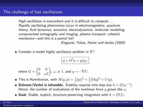
High oscillation is everywhere and it is difficult to compute.. . .Rapidly oscillating phenomena occur in electromagnetics, quantumtheory, fluid dynamics, acoustics, electrodynamics, molecular modelling,computerised tomography and imaging, plasma transport, celestialmechanics—and this is a partial list!

Engquist, Fokas, Hairer and Iserles (2009)

Consider a model highly oscillatory problem in Rd:

q + Ω2q = g(q),

where Ω =

(0 00 ωI

), ω 1, and g = −∇U .

This is Hamiltonian, with H(q, p) = 12‖p‖2 + 1

2‖Ωq‖2 + U(q).

Stormer/Verlet is infeasible. Stability requires time step size h = O(ω−1).Hence, the number of evaluations of the nonlinear force g grows like ω.

Goal: Stable, explicit, structure-preserving integrators with h = O(1).



Kinetic-potential splitting and the Stormer/Verlet method

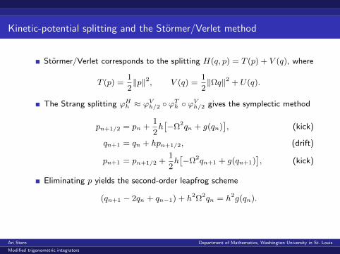
Stormer/Verlet corresponds to the splitting H(q, p) = T (p) + V (q), where

T (p) =1

2‖p‖2, V (q) =

1

2‖Ωq‖2 + U(q).

The Strang splitting ϕHh ≈ ϕVh/2 ϕTh ϕVh/2 gives the symplectic method

pn+1/2 = pn +1

2h[−Ω2qn + g(qn)

], (kick)

qn+1 = qn + hpn+1/2, (drift)

pn+1 = pn+1/2 +1

2h[−Ω2qn+1 + g(qn+1)

], (kick)

Eliminating p yields the second-order leapfrog scheme

(qn+1 − 2qn + qn−1) + h2Ω2qn = h2g(qn).



Fast-slow splitting and the impulse method

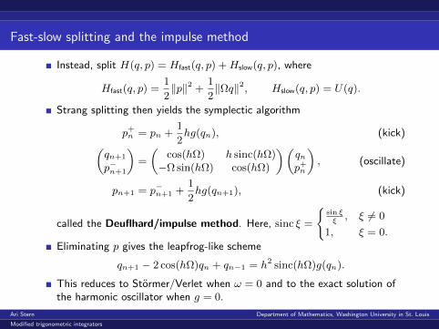
Instead, split H(q, p) = Hfast(q, p) +Hslow(q, p), where

Hfast(q, p) =1

2‖p‖2 +

1

2‖Ωq‖2, Hslow(q, p) = U(q).

Strang splitting then yields the symplectic algorithm

p+n = pn +1

2hg(qn), (kick)(

qn+1

p−n+1

)=

(cos(hΩ) h sinc(hΩ)−Ω sin(hΩ) cos(hΩ)

)(qnp+n

), (oscillate)

pn+1 = p−n+1 +1

2hg(qn+1), (kick)

called the Deuflhard/impulse method. Here, sinc ξ =

sin ξξ, ξ 6= 0

1, ξ = 0.

Eliminating p gives the leapfrog-like scheme

qn+1 − 2 cos(hΩ)qn + qn−1 = h2 sinc(hΩ)g(qn).

This reduces to Stormer/Verlet when ω = 0 and to the exact solution ofthe harmonic oscillator when g = 0.



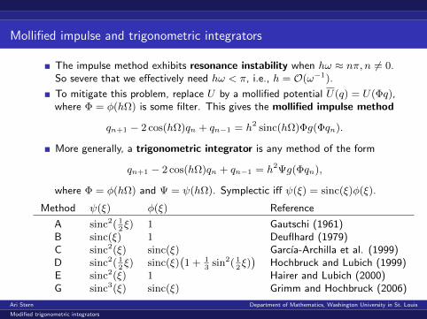
Mollified impulse and trigonometric integrators

The impulse method exhibits resonance instability when hω ≈ nπ, n 6= 0.So severe that we effectively need hω < π, i.e., h = O(ω−1).

To mitigate this problem, replace U by a mollified potential U(q) = U(Φq),where Φ = φ(hΩ) is some filter. This gives the mollified impulse method

qn+1 − 2 cos(hΩ)qn + qn−1 = h2 sinc(hΩ)Φg(Φqn).

More generally, a trigonometric integrator is any method of the form

qn+1 − 2 cos(hΩ)qn + qn−1 = h2Ψg(Φqn),

where Φ = φ(hΩ) and Ψ = ψ(hΩ). Symplectic iff ψ(ξ) = sinc(ξ)φ(ξ).

Method ψ(ξ) φ(ξ) Reference

A sinc2( 12ξ) 1 Gautschi (1961)

B sinc(ξ) 1 Deuflhard (1979)C sinc2(ξ) sinc(ξ) Garcıa-Archilla et al. (1999)D sinc2( 1

2ξ) sinc(ξ)

(1 + 1

3sin2( 1

2ξ))

Hochbruck and Lubich (1999)E sinc2(ξ) 1 Hairer and Lubich (2000)G sinc3(ξ) sinc(ξ) Grimm and Hochbruck (2006)




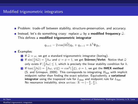
Problem: trade-off between stability, structure-preservation, and accuracy.

Instead, let’s do something crazy: replace ω by a modified frequency ω.This defines a modified trigonometric integrator

qn+1 − 2 cos(hΩ)qn + qn−1 = h2Ψgn.

Examples:1 If ω = ω, we get a standard trigonometric integrator (boring).

2 If sin( 12hω) = 1

2hω and ψ = φ = 1, we get Stormer/Verlet. Notice that ω

only exists if | 12hω| ≤ 1, which is precisely the linear stability condition for h.

3 If tan( 12hω) = 1

2hω, ψ(ξ) = cos2( 1

2ξ), φ = 1, we get the IMEX method

(S. and Grinspun, 2009). This corresponds to integrating Hfast with implicitmidpoint rather than finding the exact solution. Equivalently, a variationalintegrator using the trapezoid rule for Lslow and midpoint rule for Lfast.No resonance instability, since arctan: R→ (−π

2, π2).



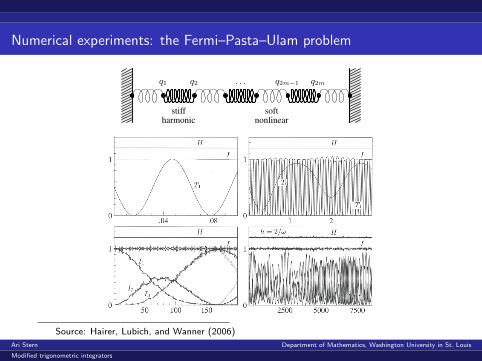
Numerical experiments: the Fermi–Pasta–Ulam problem

I.5 Highly Oscillatory Problems 21

but the symplectic Euler and the Verlet methods show the desired behaviour. Thistime a reduction of the step size does not reduce the amplitude of the oscillations,which indicates that the fluctuation of the exact temperature is of the same size.

I.5 Highly Oscillatory Problems

In this section we discuss a system with almost-harmonic high-frequency oscilla-tions. We show numerical phenomena of methods applied with step sizes that arenot small compared to the period of the fastest oscillations.

I.5.1 A Fermi–Pasta–Ulam Problem

. . . dealing with the behavior of certain nonlinear physical systems wherethe non-linearity is introduced as a perturbation to a primarily linear prob-lem. The behavior of the systems is to be studied for times which are longcompared to the characteristic periods of the corresponding linear prob-lems. (E. Fermi, J. Pasta, S. Ulam 1955)

In the early 1950s MANIAC-I had just been completed and sat poisedfor an attack on significant problems. ... Fermi suggested that it wouldbe highly instructive to integrate the equations of motion numerically fora judiciously chosen, one-dimensional, harmonic chain of mass pointsweakly perturbed by nonlinear forces. (J. Ford 1992)

The problem of Fermi, Pasta & Ulam (1955) is a simple model for simulations instatistical mechanics which revealed highly unexpected dynamical behaviour. Weconsider a modification consisting of a chain of 2m mass points, connected with al-ternating soft nonlinear and stiff linear springs, and fixed at the end points (see Gal-gani, Giorgilli, Martinoli & Vanzini (1992) and Fig. 5.1). The variables q1, . . . , q2m

q1 q2 q2m−1 q2m· · ·

stiffharmonic

softnonlinear

Fig. 5.1. Chain with alternating soft nonlinear and stiff linear springs

(q0 = q2m+1 = 0) stand for the displacements of the mass points, and pi = qi fortheir velocities. The motion is described by a Hamiltonian system with total energy

H(p, q) =1

2

m∑

i=1

(p22i−1 + p2

2i

)+

ω2

4

m∑

i=1

(q2i − q2i−1)2 +

m∑

i=0

(q2i+1 − q2i)4,

where ω is assumed to be large. It is quite natural to introduce the new variables

Source: Hairer, Lubich, and Wanner (2006)



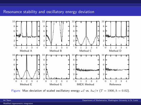
Resonance stability and oscillatory energy deviation

0 1 2 3 40

2

4

6

8

10

Method A0 1 2 3 4

0

2

4

6

8

10

Method B0 1 2 3 4

0

2

4

6

8

10

Method C0 1 2 3 4

0

2

4

6

8

10

Method D

0 1 2 3 40

2

4

6

8

10

Method E0 1 2 3 4

0

2

4

6

8

10

Method G0 1 2 3 4

0

2

4

6

8

10

IMEX Method0 1 2 3 4

0

2

4

6

8

10

Reference

Figure: Max deviation of scaled oscillatory energy ωI vs. hω/π (T = 1000, h = 0.02).



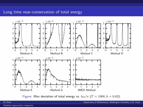
Long time near-conservation of total energy

0 1 2 3 40

1

2

3

4

5×10−3

Method A0 1 2 3 4

0

1

2

3

4

5×10−2

Method B0 1 2 3 4

0

1

2

3

4

5×10−2

Method C0 1 2 3 4

0

1

2

3

4

5×10−3

Method D

0 1 2 3 40

1

2

3

4

5×10−2

Method E0 1 2 3 4

0

1

2

3

4

5×10−2

Method G0 1 2 3 4

0

1

2

3

4

5×10−3

IMEX Method

Figure: Max deviation of total energy vs. hω/π (T = 1000, h = 0.02).



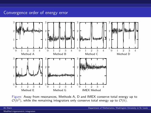
Convergence order of energy error

0 1 2 3 40

1

2

3

Method A0 1 2 3 4

0

1

2

3

Method B0 1 2 3 4

0

1

2

3

Method C0 1 2 3 4

0

1

2

3

Method D

0 1 2 3 40

1

2

3

Method E0 1 2 3 4

0

1

2

3

Method G0 1 2 3 4

0

1

2

3

IMEX Method

Figure: Away from resonances, Methods A, D and IMEX conserve total energy up toO(h2), while the remaining integrators only conserve total energy up to O(h).



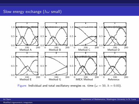
Slow energy exchange (hω small)

0 100 2000.0

0.5

1.0

Method A0 100 200

0.0

0.5

1.0

Method B0 100 200

0.0

0.5

1.0

Method C0 100 200

0.0

0.5

1.0

Method D

0 100 2000.0

0.5

1.0

Method E0 100 200

0.0

0.5

1.0

Method G0 100 200

0.0

0.5

1.0

IMEX Method0 100 200

0.0

0.5

1.0

Reference

Figure: Individual and total oscillatory energies vs. time (ω = 50, h = 0.03).



Slow energy exchange (hω larger)

0 100 2000.0

0.5

1.0

Method A0 100 200

0.0

0.5

1.0

Method B0 100 200

0.0

0.5

1.0

Method C0 100 200

0.0

0.5

1.0

Method D

0 100 2000.0

0.5

1.0

Method E0 100 200

0.0

0.5

1.0

Method G0 100 200

0.0

0.5

1.0

IMEX Method0 100 200

0.0

0.5

1.0

Reference




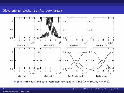
Slow energy exchange (hω very large)

0 1 2 3 4×104

0.0

0.5

1.0

Method A

0 1 2 3 4×104

0.0

0.5

1.0

Method B

0 1 2 3 4×104

0.0

0.5

1.0

Method C

0 1 2 3 4×104

0.0

0.5

1.0

Method D

0 1 2 3 4×104

0.0

0.5

1.0

Method E

0 1 2 3 4×104

0.0

0.5

1.0

Method G

0 1 2 3 4×104

0.0

0.5

1.0

IMEX Method

0 1 2 3 4×104

0.0

0.5

1.0

Reference




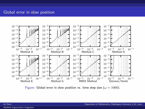
Global error in slow position

10−3 10−2 10−110−7

10−6

10−5

10−4

10−3

10−2

Method A10−3 10−2 10−1

10−7

10−6

10−5

10−4

10−3

10−2

Method B10−3 10−2 10−1

10−7

10−6

10−5

10−4

10−3

10−2

Method C10−3 10−2 10−1

10−7

10−6

10−5

10−4

10−3

10−2

Method D

10−3 10−2 10−110−7

10−6

10−5

10−4

10−3

10−2

Method E10−3 10−2 10−1

10−7

10−6

10−5

10−4

10−3

10−2

Method G10−3 10−2 10−1

10−7

10−6

10−5

10−4

10−3

10−2

IMEX Method10−3 10−2 10−1

10−7

10−6

10−5

10−4

10−3

10−2

Stormer/Verlet

Figure: Global error in slow position vs. time step size (ω = 1000).



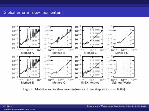
Global error in slow momentum

10−3 10−2 10−110−7

10−6

10−5

10−4

10−3

10−2

Method A10−3 10−2 10−1

10−7

10−6

10−5

10−4

10−3

10−2

Method B10−3 10−2 10−1

10−7

10−6

10−5

10−4

10−3

10−2

Method C10−3 10−2 10−1

10−7

10−6

10−5

10−4

10−3

10−2

Method D

10−3 10−2 10−110−7

10−6

10−5

10−4

10−3

10−2

Method E10−3 10−2 10−1

10−7

10−6

10−5

10−4

10−3

10−2

Method G10−3 10−2 10−1

10−7

10−6

10−5

10−4

10−3

10−2

IMEX Method10−3 10−2 10−1

10−7

10−6

10−5

10−4

10−3

10−2

Stormer/Verlet

Figure: Global error in slow momentum vs. time step size (ω = 1000).



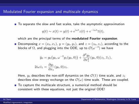
Modulated Fourier expansion and multiscale dynamics

To separate the slow and fast scales, take the asymptotic approximation

q(t) ∼ x(t) = y(t) + eiωtz(t) + e−iωtz(t),

which are the principal terms of the modulated Fourier expansion.

Decomposing x = (x0, x1), y = (y0, y1), and z = (z0, z1), according to theblocks of Ω, and plugging into the ODE, up to O(ω−3) we have

y0 = g0(y0, ω

−2g1(y0, 0))

+∂2g0∂x21

(y0, 0)(z1, z1),

2iωz1 =∂g1∂x1

(y0, 0)z1.

Here, y0 describes the non-stiff dynamics on the O(1) time scale, and z1describes slow energy exchange on the O(ω) time scale. These are coupled.

To capture the multiscale structure, a numerical method should beconsistent with these equations, not just the original ODE!



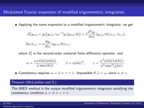
Modulated Fourier expansion of modified trigonometric integrators

Applying the same expansion to a modified trigonometric integrator, we get

δ2hyh,0 = g0(yh,0, γω

−2g1(yh,0, 0))

+ β∂2g0∂x21

(yh,0, 0)(zh,1, zh,1),

2iωzh,1 = α∂g1∂x1

(yh,0, 0)zh,1,

where δ2h is the second-order centered finite difference operator, and

α =ωψ(hω)φ(hω)

ω sinc(hω), β = φ(hω)2, γ =

ω2ψ(hω)φ(hω)

ω2 sinc2( 12hω)

.

Consistency requires α = β = γ = 1. Impossible if ω = ω, since α 6= γ.

Theorem (McLachlan and S.)

The IMEX method is the unique modified trigonometric integrator satisfying theconsistency condition α = β = γ = 1.



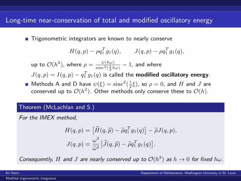
Long-time near-conservation of total and modified oscillatory energy

Trigonometric integrators are known to nearly conserve

H(q, p)− ρqT1 g1(q), J(q, p)− ρqT1 g1(q),

up to O(h2), where ρ = ψ(hω)

sinc2( 12hω)− 1, and where

J(q, p) = I(q, p)− qT1 g1(q) is called the modified oscillatory energy.

Methods A and D have ψ(ξ) = sinc2( 12ξ), so ρ = 0, and H and J are

conserved up to O(h2). Other methods only conserve these to O(h).

Theorem (McLachlan and S.)

For the IMEX method,

H(q, p) =[H(q, p)− ρqT1 g1(q)

]− ρJ(q, p),

J(q, p) =ω2

ω2

[J(q, p)− ρqT1 g1(q)

].

Consequently, H and J are nearly conserved up to O(h2) as h→ 0 for fixed hω.



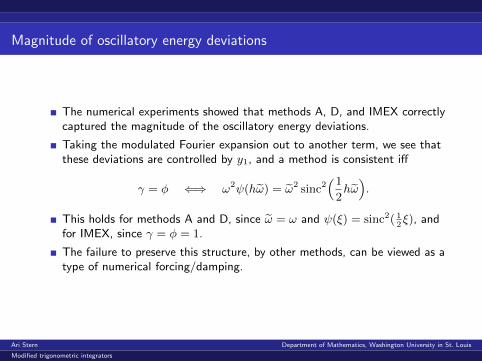
Magnitude of oscillatory energy deviations

The numerical experiments showed that methods A, D, and IMEX correctlycaptured the magnitude of the oscillatory energy deviations.

Taking the modulated Fourier expansion out to another term, we see thatthese deviations are controlled by y1, and a method is consistent iff

γ = φ ⇐⇒ ω2ψ(hω) = ω2 sinc2(1

2hω).

This holds for methods A and D, since ω = ω and ψ(ξ) = sinc2( 12ξ), and

for IMEX, since γ = φ = 1.

The failure to preserve this structure, by other methods, can be viewed as atype of numerical forcing/damping.



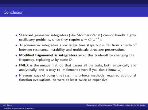
Conclusion

Standard geometric integrators (like Stormer/Verlet) cannot handle highlyoscillatory problems, since they require h = O(ω−1).

Trigonometric integrators allow larger time steps but suffer from a trade-offbetween resonance instability and multiscale structure preservation.

Modified trigonometric integrators avoid this trade-off by changing thefrequency, replacing ω by some ω.

IMEX is the unique method that passes all the tests, both empirically andanalytically, and is easy to implement (even if you don’t know ω).

Previous ways of doing this (e.g., multi-force methods) required additionalfunction evaluations, so were at least twice as expensive.



Date post:	25-Feb-2022
Category:	Documents
Upload:	others
View:	0 times
Download:	0 times

Modi ed trigonometric integrators - NTNU

Documents