82
Modul Layout and Design Prof. Dr. Richard F. Hartl Dr. Margaretha Gansterer SS 2010 © Produktion und Logistik
Modul
Layout and Design
Prof. Dr. Richard F. Hartl
Dr. Margaretha Gansterer
SS 2010
© Produktion und Logistik
Hartl, Gansterer Layout and Design 2
© Produktion und Logistik
Contents
0. Introduction ..................................................................................................................... 5
1. Methodological Basics ..................................................................................................... 9
Complexity ........................................................................................................................ 9
Costs and distances ......................................................................................................... 10
Basics on Graph Theory .................................................................................................. 11
2. Job shop production ..................................................................................................... 13
2.1. The Linear Assignment Problem ............................................................................. 14
2.1.1. Formulation as transportation problem ........................................................ 15
2.1.2. Assignment Method (Kuhn’s Algorithm) .................................................... 17
2.2. The Quadratic Assignment Problem (QAP) ............................................................ 22
2.2.1. QAP: Mathematical formulation .................................................................. 24
2.2.2. Starting heuristics ......................................................................................... 26 2.2.3. Improvement methods .................................................................................. 27
2.2.4. „Umlaufmethode“ ........................................................................................ 28
2.2.5. Different space requirements........................................................................ 30
2.2.5.1. CRAFT Algorithm .................................................................. 31
3. Group Technology / Cellular Manufacturing ............................................................ 38
3.1 Introduction ............................................................................................................... 38
3.2 How to form groups .................................................................................................. 41
3.3 Coding schemes ........................................................................................................ 42
3.4 Classification (group formation) ............................................................................... 45
3.5 Production Flow Analysis (PFA) .............................................................................. 45
3.5.1 Binary Ordering (Rank Order Clustering, King’s Algorithm) ........................ 47
3.5.2 Single-Pass Heuristic Considering Capacities (Askin and Standridge) .......... 50
3.5.3 LP-Model for the model by Askin and Standridge ......................................... 52
3.5.4. Clustering using Similarity Coefficients ........................................................ 54
3.5.5. Group Formation using Graph Partitioning ................................................... 57
3.5.6 Group analysis without binary ordering: “key" machine ................................ 65
3.6 Metaheuristics ........................................................................................................... 67
References ....................................................................................................................... 67
4. Exact Methods for Assembly Line Balancing ............................................................. 69
Hartl, Gansterer Layout and Design 3
© Produktion und Logistik
Jackson Algorithm (Dynamic Programming, Decision Tree) .................................. 69
The B&B algorithm by Johnson von (FABLE) ....................................................... 75
Hartl, Gansterer Layout and Design 4
© Produktion und Logistik
Hartl, Gansterer Layout and Design 5
© Produktion und Logistik
0. Introduction 12
Layout decisions are one of the key facts determining the long-run efficiency of operations. Layouts have numerous strategic implications because they establish an organization´s competitive priorities in regard to capacity, processes, flexibility, and cost. They are associated with the tactical decision horizon and are dedicated to the concretion of strategic decisions like, e.g., facility location. Configured production systems are input for the operational level, where the goal is to run the given system as efficiently a possible.
An efficient layout facilitates and reduces costs of material flow, people, and information between areas. To achieve these objectives, a variety of configuration designs have been developed. The most relevant ones, in the context of this course, are:
1. Fixed-position layout: addresses the layout requirements of large, bulky projects
2. Job shop production (Process-oriented layout): deals with low-volume, high-variety production
3. Cellular manufacturing systems (work cell layout): arranges machinery and equipment to focus on production of a single product or group of related products
4. Flow shop production (Product-oriented layout): seeks the best personnel and machine utilization in repetitive or continuous production.
As a matter of fact layouts 1 and 2 are often described as centralized, and layouts 3 and 4 as decentralized manufacturing systems.
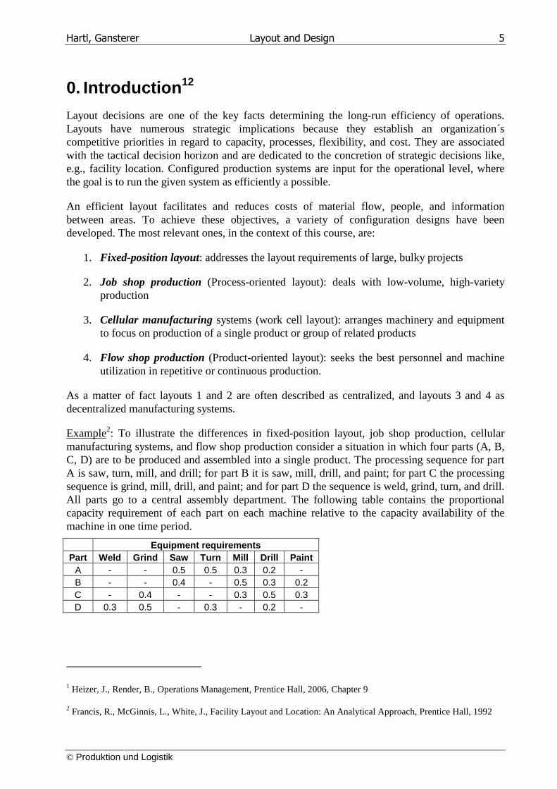
Example2: To illustrate the differences in fixed-position layout, job shop production, cellular manufacturing systems, and flow shop production consider a situation in which four parts (A, B, C, D) are to be produced and assembled into a single product. The processing sequence for part A is saw, turn, mill, and drill; for part B it is saw, mill, drill, and paint; for part C the processing sequence is grind, mill, drill, and paint; and for part D the sequence is weld, grind, turn, and drill. All parts go to a central assembly department. The following table contains the proportional capacity requirement of each part on each machine relative to the capacity availability of the machine in one time period.
Equipment requirements Part Weld Grind Saw Turn Mill Drill Paint
A - - 0.5 0.5 0.3 0.2 - B - - 0.4 - 0.5 0.3 0.2 C - 0.4 - - 0.3 0.5 0.3 D 0.3 0.5 - 0.3 - 0.2 -
1 Heizer, J., Render, B., Operations Management, Prentice Hall, 2006, Chapter 9
2 Francis, R., McGinnis, L., White, J., Facility Layout and Location: An Analytical Approach, Prentice Hall, 1992
Hartl, Gansterer Layout and Design 6
© Produktion und Logistik
Based on the given capacity requirements we know that the minimum equipment needed is: 1 weld, 1 grind, 1 saw, 1 turning machine, 2 mills (0.3+0.5+0.3 > 1), 2 drills, and 1 painting machine.
According to the layout concepts listed above the following configurations for the example problem could be realized (this is not a complete list of all possible configurations but an illustrative selection of possible realizations).
1. In case of a fixed-position layout it may be sufficient to have the minimum machine equipment (see above). But depending on how production is scheduled it could also be necessary to install more machines in order to come up with the needed production output.
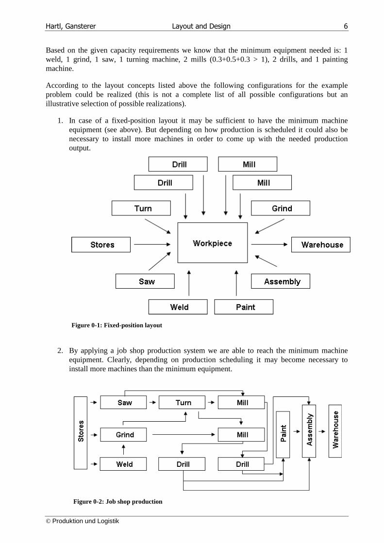
2. By applying a job shop production system we are able to reach the minimum machine equipment. Clearly, depending on production scheduling it may become necessary to install more machines than the minimum equipment.
Figure 0-1: Fixed-position layout
Figure 0-2: Job shop production
Hartl, Gansterer Layout and Design 7
© Produktion und Logistik
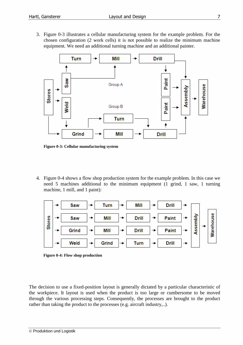
3. Figure 0-3 illustrates a cellular manufacturing system for the example problem. For the chosen configuration (2 work cells) it is not possible to realize the minimum machine equipment. We need an additional turning machine and an additional painter.
Figure 0-3: Cellular manufacturing system
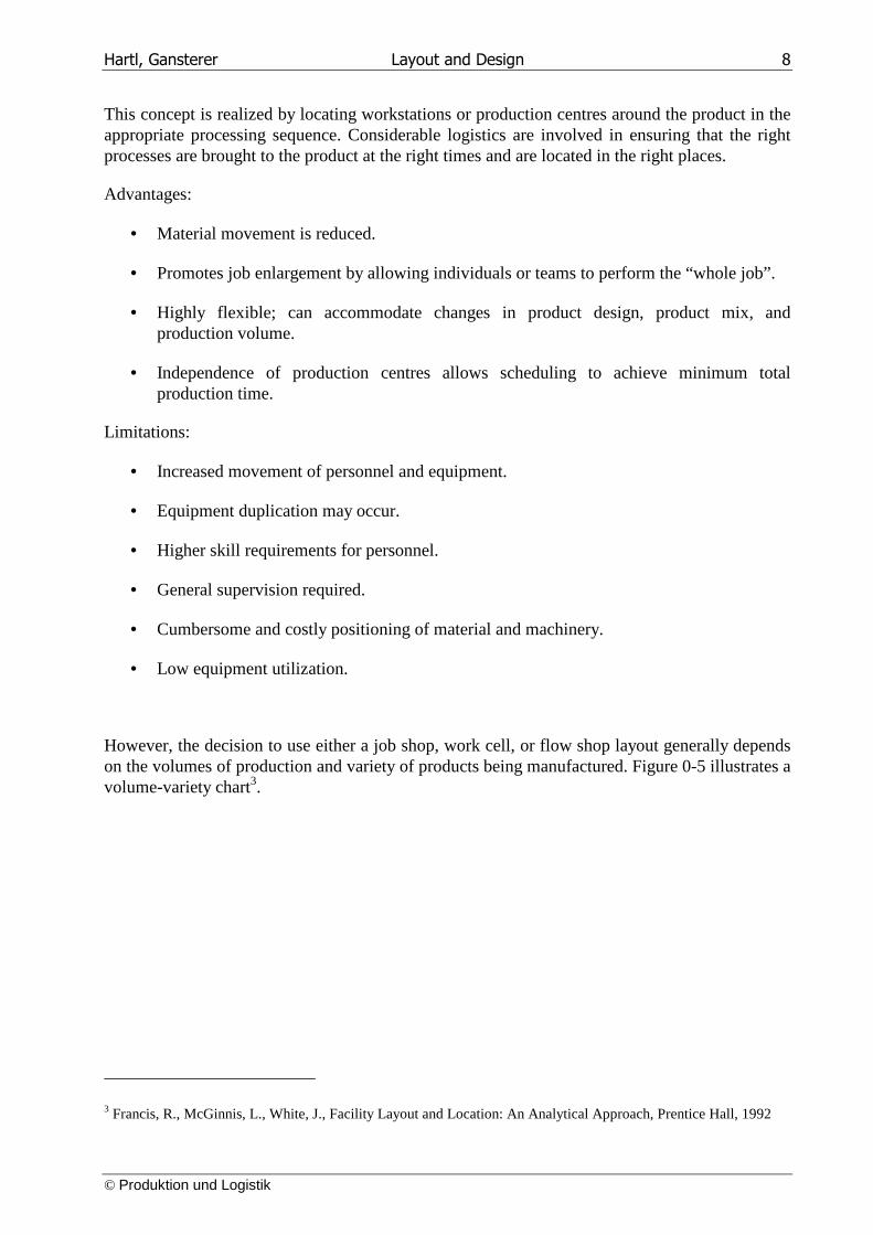
4. Figure 0-4 shows a flow shop production system for the example problem. In this case we need 5 machines additional to the minimum equipment (1 grind, 1 saw, 1 turning machine, 1 mill, and 1 paint):
Figure 0-4: Flow shop production
The decision to use a fixed-position layout is generally dictated by a particular characteristic of the workpiece. It layout is used when the product is too large or cumbersome to be moved through the various processing steps. Consequently, the processes are brought to the product rather than taking the product to the processes (e.g. aircraft industry,..).
Hartl, Gansterer Layout and Design 8
© Produktion und Logistik
This concept is realized by locating workstations or production centres around the product in the appropriate processing sequence. Considerable logistics are involved in ensuring that the right processes are brought to the product at the right times and are located in the right places.
Advantages:
• Material movement is reduced.
• Promotes job enlargement by allowing individuals or teams to perform the “whole job”.
• Highly flexible; can accommodate changes in product design, product mix, and production volume.
• Independence of production centres allows scheduling to achieve minimum total production time.
Limitations:
• Increased movement of personnel and equipment.
• Equipment duplication may occur.
• Higher skill requirements for personnel.
• General supervision required.
• Cumbersome and costly positioning of material and machinery.
• Low equipment utilization.
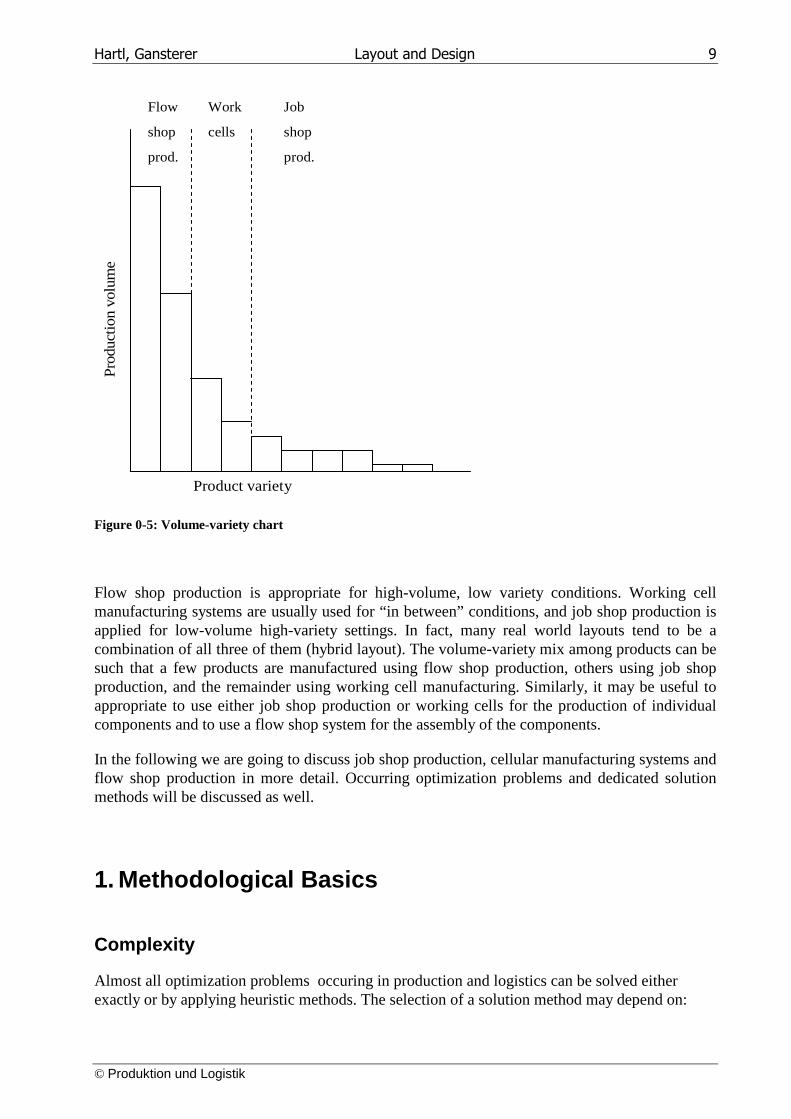
However, the decision to use either a job shop, work cell, or flow shop layout generally depends on the volumes of production and variety of products being manufactured. Figure 0-5 illustrates a volume-variety chart3.
3 Francis, R., McGinnis, L., White, J., Facility Layout and Location: An Analytical Approach, Prentice Hall, 1992
Hartl, Gansterer Layout and Design 9
© Produktion und Logistik
Product variety
Pro
duct
ion
volu
me
Flow
shop
prod.
Work
cells
Job
shop
prod.
Figure 0-5: Volume-variety chart
Flow shop production is appropriate for high-volume, low variety conditions. Working cell manufacturing systems are usually used for “in between” conditions, and job shop production is applied for low-volume high-variety settings. In fact, many real world layouts tend to be a combination of all three of them (hybrid layout). The volume-variety mix among products can be such that a few products are manufactured using flow shop production, others using job shop production, and the remainder using working cell manufacturing. Similarly, it may be useful to appropriate to use either job shop production or working cells for the production of individual components and to use a flow shop system for the assembly of the components.
In the following we are going to discuss job shop production, cellular manufacturing systems and flow shop production in more detail. Occurring optimization problems and dedicated solution methods will be discussed as well.
1. Methodological Basics
Complexity
Almost all optimization problems occuring in production and logistics can be solved either exactly or by applying heuristic methods. The selection of a solution method may depend on:

Hartl, Gansterer Layout and Design 10
© Produktion und Logistik
● Software availability
● Cost-benefit
● Problem complexity
Even if we know adequate (time consuming) exact methods we are going to apply heuristic methods if we do not have adequate software available or costs (installation, personnel instruction, etc.) exceed the expected benefit.
On the other hand we know a number of combinatorial problems, which are classified to be „NP-hard“, which indicates the assumption that the computational effort for solving the problem will not increase polynomial with the problem dimension. In case of real-world applications with the according problem size we face unacceptable computational times, even for high performance IT-systems, regularly.
LP-Problems (average case) are to be solved with polynomial effort, since the number of simplex-iterations increases linearly with the number of constraints (and each iteration causes quadratic effort).
LP-Problems with integer variables usually are solved by applying a Branch and Bound (B&B) method, where a common LP-model is solved in each iteration. Here the number of iterations increases exponentially with the number of integer variables. Thus, these problems cannot be solved with polynomial effort.
For some problem classes (e.g. transportation problems, (linear) assignment) due to their problem structure integer/binary property of the decision variables is guaranteed automatically leading to a low problem complexity.
Some problems with integer/binary variables can (by using special exact methods) be solved with polynomial effort, anyway.
Referring to heuristic methods we usually distinguish between:
● Starting heuristics (quick generation of a feasible solution)
● Improvement heuristics (start with a feasible solution and try to find a better one)
● Combinations of starting and improvement heuristics
We use “general purpose”-heuristics or metaheuristics (e.g. Simulated Annealing, Tabu Search or Genetic Algortihms) in order to leave local optima during improvement steps.
Costs and distances
The majority of problems being dealt with during this course will be solved based on costs and/or distances cij. In most cases costs are determined based on given technical parameters (machine setup,..) or distances (e.g. distance between object i and j). In the following we are going to introduce three common distances:
Hartl, Gansterer Layout and Design 11
© Produktion und Logistik
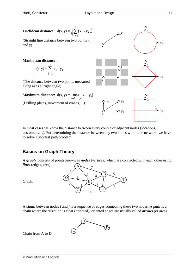
Euclidean distance: ( )d(x,y) = x - yi ii=1
n2∑
(Straight line distance between two points x and y)
x
y
x2
x1 1
1
Manhattan distance:
d(x,y) = x - yi ii =1
n
∑
(The distance between two points measured along axes at right angle)
y
x
x2
x1 1
1
Maximum distance: d(x, y) = max x - yi=1,...,n
i i
(Drilling plates, movement of cranes,…)
x y1
y2 y3
x2
x1 1
1
In most cases we know the distance between every couple of adjacent nodes (locations, customers,…). For determining the distance between any two nodes within the network, we have to solve a shortest path problem.
Basics on Graph Theory
A graph consists of points known as nodes (vertices) which are connected with each other using lines (edges, arcs).
Graph:
A chain between nodes I and j is a sequence of edges connecting these two nodes. A path is a chain where the direction is clear (oriented); oriented edges are usually called arrows (or arcs).
Chain from A to D:
O
A
C
B
E
D
T
4
2
52
7
4 5
71
3
4
1
Hartl, Gansterer Layout and Design 12
© Produktion und Logistik
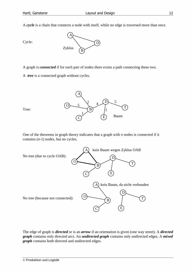
A cycle is a chain that connects a node with itself, while no edge is traversed more than once.
Cycle:
A graph is connected if for each pair of nodes there exists a path connecting these two.
A tree is a connected graph without cycles.
Tree:
One of the theorems in graph theory indicates that a graph with n nodes is connected if it contains (n-1) nodes, but no cycles.
No tree (due to cycle OAB):
No tree (because not connected):
The edge of graph is directed or is an arrow if an orientation is given (one way street). A directed graph contains only directed arcs. An undirected graph contains only undirected edges. A mixed graph contains both directed and undirected edges.
A
B
DZyklus
O
A
C
B
E
D
T52 4 5
11
Baum
O
A
C
B
E
D
T
kein Baum wegen Zyklus OAB
O
A
C
B
E
D
T
kein Baum, da nicht verbunden
Hartl, Gansterer Layout and Design 13
© Produktion und Logistik
2. Job shop production 45
The process-oriented layout can simultaneously handle a wide variety of products. It is typically the low-volume, high-variety strategy. Each product or product group undergoes a different sequence of operations. It is produced moving it from one department to another in the required sequence. Different products have different material flows. Thus, it is not efficient to arrange machines due to a product-oriented layout (flow shop system) but according to a process-oriented layout.
A process-oriented layout consists of a collection of processing departments or cells. All machines involved in performing a particular process are grouped together in a machine shop (e.g. drill, weld,..). This concept is used when there are many low-volume, dissimilar products. It is also used in case of rapid changes in product mix or volume, as well as when conditions are such that neither product-oriented nor cellular manufacturing systems are useful. In comparison with cellular manufacturing systems this layout concept is characterized by high degrees of interdepartmental flow. A big advantage of this process-oriented layout is its flexibility in equipment and labor assignment. The breakdown of one machine need not halt an entire process; work can be transferred to other machines in the department.
Advantages:
• Better utilization of machines can result; consequently, fewer machines are required.
• A high degree of flexibility exists relative to equipment or manpower allocation for specific tasks.
• Comparatively low investment in machines is required.
• The diversity of tasks offers a more interesting and satisfying occupation for the operator.
• Specialized supervision is possible.
Limitations:
• Since longer flow lines are needed, material handling is more expensive.
• Production planning and control systems are more involved than for other layouts.
• Usually, total production time is longer than for other layouts.
4 Heizer, J., Render, B., Operations Management, Prentice Hall, 2006, Chapter 9
5 Francis, R., McGinnis, L., White, J., Facility Layout and Location: An Analytical Approach, Prentice Hall, 1992
Hartl, Gansterer Layout and Design 14
© Produktion und Logistik
• Due to the fact that jobs have to queue before being processed in a machine job comparatively large amounts of in-process inventory occur.
• Comparatively high degree of (machine) idle time because machines have to wait until the subsequent job is finished with its foregoing process.
• Space and capital are tied up by work in process.
• Because of the diversity of the jobs in specialized departments, higher grades of skill are required.
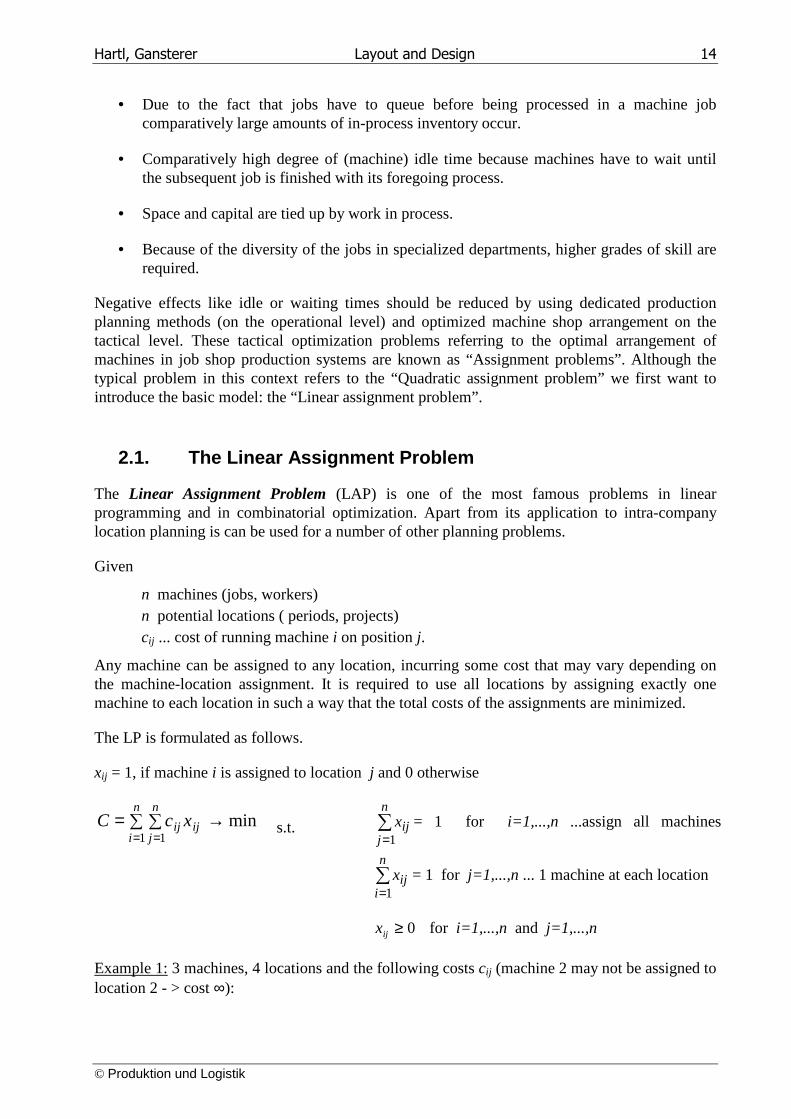
Negative effects like idle or waiting times should be reduced by using dedicated production planning methods (on the operational level) and optimized machine shop arrangement on the tactical level. These tactical optimization problems referring to the optimal arrangement of machines in job shop production systems are known as “Assignment problems”. Although the typical problem in this context refers to the “Quadratic assignment problem” we first want to introduce the basic model: the “Linear assignment problem”.
2.1. The Linear Assignment Problem
The Linear Assignment Problem (LAP) is one of the most famous problems in linear programming and in combinatorial optimization. Apart from its application to intra-company location planning is can be used for a number of other planning problems.
Given
n machines (jobs, workers) n potential locations ( periods, projects) cij ... cost of running machine i on position j.
Any machine can be assigned to any location, incurring some cost that may vary depending on the machine-location assignment. It is required to use all locations by assigning exactly one machine to each location in such a way that the total costs of the assignments are minimized.
The LP is formulated as follows.
xij = 1, if machine i is assigned to location j and 0 otherwise
min1 1
→∑ ∑== =
n
iij
n
jij xcC s.t. ∑
=
n
jijx
1= 1 for i=1,...,n ...assign all machines
∑=
n
iijx
1= 1 for j=1,...,n ... 1 machine at each location
0≥ijx for i=1,...,n and j=1,...,n
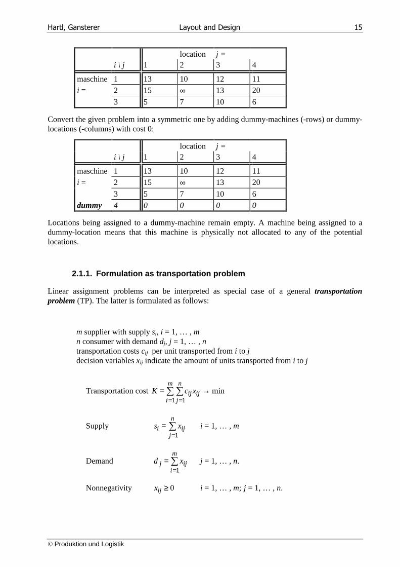
Example 1: 3 machines, 4 locations and the following costs cij (machine 2 may not be assigned to location 2 - > cost ∞):
Hartl, Gansterer Layout and Design 15
© Produktion und Logistik
location j = i \ j 1 2 3 4
maschine 1 13 10 12 11
i = 2 15 ∞ 13 20
3 5 7 10 6
Convert the given problem into a symmetric one by adding dummy-machines (-rows) or dummy-locations (-columns) with cost 0:
location j = i \ j 1 2 3 4
maschine 1 13 10 12 11
i = 2 15 ∞ 13 20
3 5 7 10 6
dummy 4 0 0 0 0
Locations being assigned to a dummy-machine remain empty. A machine being assigned to a dummy-location means that this machine is physically not allocated to any of the potential locations.
2.1.1. Formulation as transportation problem
Linear assignment problems can be interpreted as special case of a general transportation problem (TP). The latter is formulated as follows:
m supplier with supply si, i = 1, … , m n consumer with demand dj, j = 1, … , n transportation costs cij per unit transported from i to j decision variables xij indicate the amount of units transported from i to j
Transportation cost min1 1
→= ∑ ∑= =
m
iij
n
jij xcK
Supply ∑=
=n
jiji xs
1 i = 1, … , m
Demand ∑=
=m
iijj xd
1 j = 1, … , n.
Nonnegativity 0≥ijx i = 1, … , m; j = 1, … , n.
Hartl, Gansterer Layout and Design 16
© Produktion und Logistik
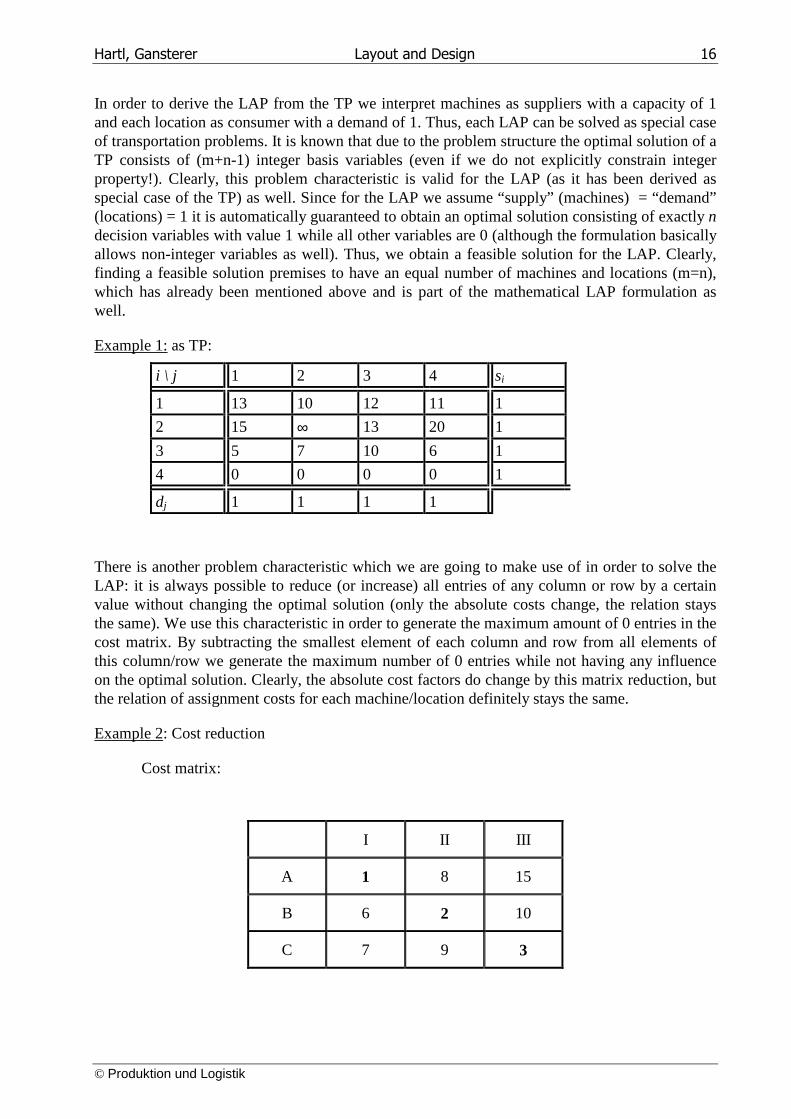
In order to derive the LAP from the TP we interpret machines as suppliers with a capacity of 1 and each location as consumer with a demand of 1. Thus, each LAP can be solved as special case of transportation problems. It is known that due to the problem structure the optimal solution of a TP consists of (m+n-1) integer basis variables (even if we do not explicitly constrain integer property!). Clearly, this problem characteristic is valid for the LAP (as it has been derived as special case of the TP) as well. Since for the LAP we assume “supply” (machines) = “demand” (locations) = 1 it is automatically guaranteed to obtain an optimal solution consisting of exactly n decision variables with value 1 while all other variables are 0 (although the formulation basically allows non-integer variables as well). Thus, we obtain a feasible solution for the LAP. Clearly, finding a feasible solution premises to have an equal number of machines and locations (m=n), which has already been mentioned above and is part of the mathematical LAP formulation as well.
Example 1: as TP:
i \ j 1 2 3 4 si
1 13 10 12 11 1
2 15 ∞ 13 20 1
3 5 7 10 6 1
4 0 0 0 0 1
dj 1 1 1 1
There is another problem characteristic which we are going to make use of in order to solve the LAP: it is always possible to reduce (or increase) all entries of any column or row by a certain value without changing the optimal solution (only the absolute costs change, the relation stays the same). We use this characteristic in order to generate the maximum amount of 0 entries in the cost matrix. By subtracting the smallest element of each column and row from all elements of this column/row we generate the maximum number of 0 entries while not having any influence on the optimal solution. Clearly, the absolute cost factors do change by this matrix reduction, but the relation of assignment costs for each machine/location definitely stays the same.
Example 2: Cost reduction
Cost matrix:
I II III
A 1 8 15
B 6 2 10
C 7 9 3
Hartl, Gansterer Layout and Design 17
© Produktion und Logistik
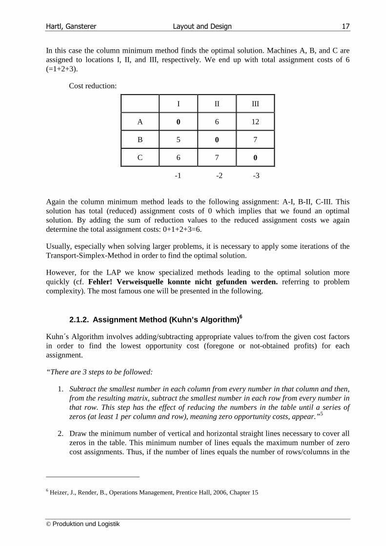
In this case the column minimum method finds the optimal solution. Machines A, B, and C are assigned to locations I, II, and III, respectively. We end up with total assignment costs of 6 (=1+2+3).
Cost reduction:
I II III
A 0 6 12
B 5 0 7
C 6 7 0
-1 -2 -3
Again the column minimum method leads to the following assignment: A-I, B-II, C-III. This solution has total (reduced) assignment costs of 0 which implies that we found an optimal solution. By adding the sum of reduction values to the reduced assignment costs we again determine the total assignment costs: 0+1+2+3=6.
Usually, especially when solving larger problems, it is necessary to apply some iterations of the Transport-Simplex-Method in order to find the optimal solution.
However, for the LAP we know specialized methods leading to the optimal solution more quickly (cf. Fehler! Verweisquelle konnte nicht gefunden werden. referring to problem complexity). The most famous one will be presented in the following.
2.1.2. Assignment Method (Kuhn’s Algorithm) 6
Kuhn´s Algorithm involves adding/subtracting appropriate values to/from the given cost factors in order to find the lowest opportunity cost (foregone or not-obtained profits) for each assignment.
“There are 3 steps to be followed:
1. Subtract the smallest number in each column from every number in that column and then, from the resulting matrix, subtract the smallest number in each row from every number in that row. This step has the effect of reducing the numbers in the table until a series of zeros (at least 1 per column and row), meaning zero opportunity costs, appear.”5
2. Draw the minimum number of vertical and horizontal straight lines necessary to cover all zeros in the table. This minimum number of lines equals the maximum number of zero cost assignments. Thus, if the number of lines equals the number of rows/columns in the
6 Heizer, J., Render, B., Operations Management, Prentice Hall, 2006, Chapter 15
Hartl, Gansterer Layout and Design 18
© Produktion und Logistik
table, then we can make an optimal assignment. If the number of lines is less than the number of rows or columns, we proceed to step 3.
At this point we want to complete this step of the Assignment Method by specifying the procedure during step 2. In fact, finding the minimum number of vertical and horizontal lines necessary to cover all zeros in a matrix may be trivial in case of very small matrices, but should be solved systematically in case of larger ones. Thus, we want to introduce the following procedure in addition to step 2:
We proceed systematically by choosing a column or row with as few as possible zero entries (preferably exactly one 0) and framing (shading) a 0 in this column or row. This leads to an interim assignment.
Then we cross all remaining zeros in this column or row. Now in each column or row related to a framed 0 all other zeros are crossed which means that in this column or row no further assignments are possible.
Now the next column or row with as few as possible non-marked (not crossed and not framed) zeros is chosen and so on. We stop as soon as we do not have zeros left to be framed. Now we have an arrangement of marked columns and rows including all zeros.
If we are able to make an assignment with (reduced) costs of 0 for each machine we have found an optimal assignment otherwise we proceed as follows:
2.1. Mark (for example „X“) all rows with no framed 0
2.2. Mark all columns having at least 1 crossed 0 in a marked row
2.3. Mark all rows having a framed 0 in a marked column
2.4. Repeat 2.2 and 2.3 until there is no column or row left to be marked
2.5. Mark each non-marked row and each marked column (shaded) with a continuous line -> all framed zeros are crossed now and we have the minimum number of crossed lines and rows needed to cover all zeros, i.e. the maximum number of zero cost assignments. If this number equals the number of rows or columns an optimal assignment is already found (in this case it would not have been necessary to perform the given subprocedure (2.1.-2.6.) because we should already have succeeded in finding a zero cost assignment as described above).
3. “Substract the smallest number not covered by a line from every other uncovered number. Add the same number to any number(s) lying at the intersection of any two lines. Do not change the value of the numbers that are covered by only one line. Return to step 2 and continue until an optimal assignment is possible.
Some assignment problems entail maximizing profit, effectiveness, or payoff of an assignment of people to tasks or of jobs to machines. It is easy to obtain an equivalent minimization problem by converting every number in the matrix to an opportunity loss. To convert a maximization problem to an equivalent minimization problem, we subtract every number in the original matrix from the largest single number in that matrix. We then proceed to step 1. It turns out that
Hartl, Gansterer Layout and Design 19
© Produktion und Logistik
minimizing the opportunity loss produces the same assignment solution as the original maximization problem.”7
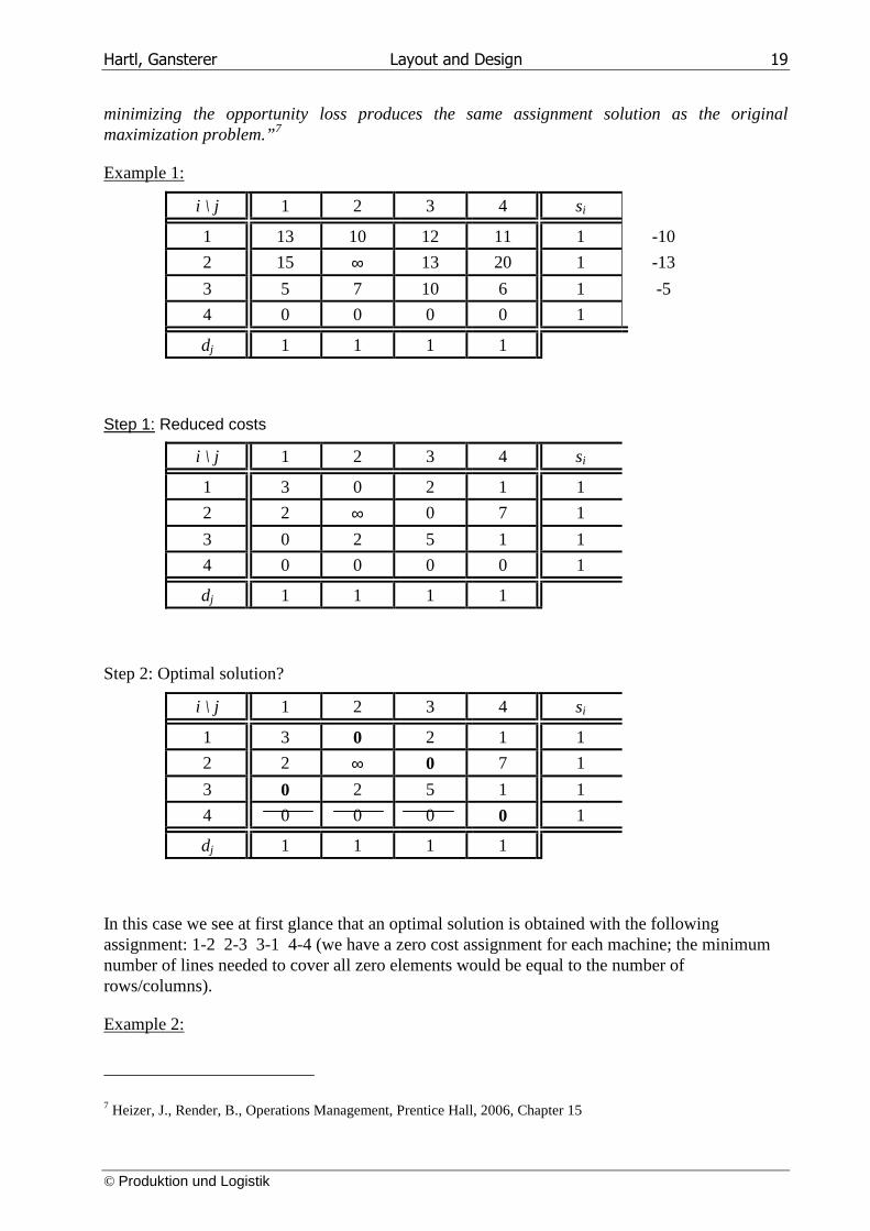
Example 1:
i \ j 1 2 3 4 si
1 13 10 12 11 1 -10
2 15 ∞ 13 20 1 -13
3 5 7 10 6 1 -5
4 0 0 0 0 1
dj 1 1 1 1
Step 1: Reduced costs
i \ j 1 2 3 4 si
1 3 0 2 1 1
2 2 ∞ 0 7 1
3 0 2 5 1 1
4 0 0 0 0 1
dj 1 1 1 1
Step 2: Optimal solution?
i \ j 1 2 3 4 si
1 3 0 2 1 1
2 2 ∞ 0 7 1
3 0 2 5 1 1
4 0 0 0 0 1
dj 1 1 1 1
In this case we see at first glance that an optimal solution is obtained with the following assignment: 1-2 2-3 3-1 4-4 (we have a zero cost assignment for each machine; the minimum number of lines needed to cover all zero elements would be equal to the number of rows/columns).
Example 2:
7 Heizer, J., Render, B., Operations Management, Prentice Hall, 2006, Chapter 15
Hartl, Gansterer Layout and Design 20
© Produktion und Logistik
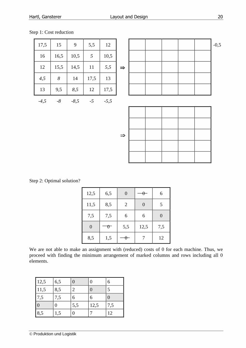
Step 1: Cost reduction
17,5 15 9 5,5 12 -0,5
16 16,5 10,5 5 10,5
12 15,5 14,5 11 5,5 ⇒⇒⇒⇒
4,5 8 14 17,5 13
13 9,5 8,5 12 17,5
-4,5 -8 -8,5 -5 -5,5
⇒⇒⇒⇒
Step 2: Optimal solution?
12,5 6,5 0 0 6
11,5 8,5 2 0 5
7,5 7,5 6 6 0
0 0 5,5 12,5 7,5
8,5 1,5 0 7 12
We are not able to make an assignment with (reduced) costs of 0 for each machine. Thus, we proceed with finding the minimum arrangement of marked columns and rows including all 0 elements.
12,5 6,5 0 0 6
11,5 8,5 2 0 5
7,5 7,5 6 6 0
0 0 5,5 12,5 7,5
8,5 1,5 0 7 12
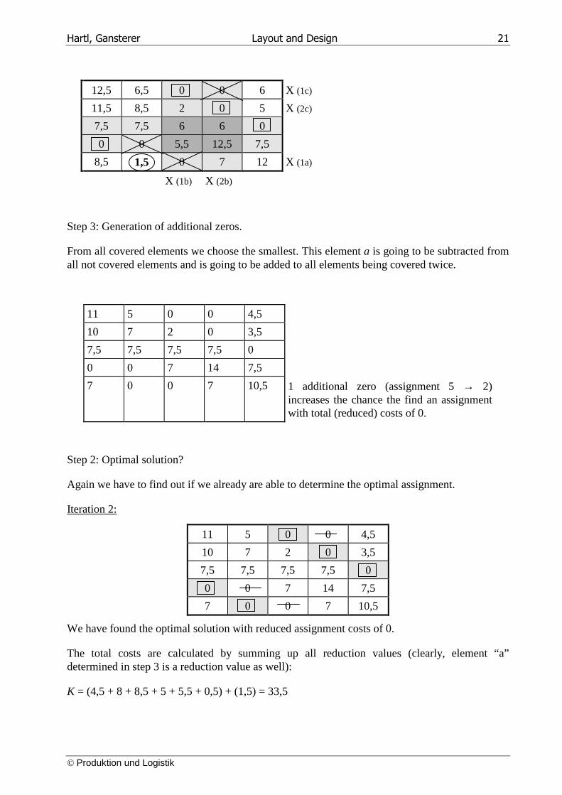
Hartl, Gansterer Layout and Design 21
© Produktion und Logistik
12,5 6,5 0 0 6 X (1c)
11,5 8,5 2 0 5 X (2c)
7,5 7,5 6 6 0
0 0 5,5 12,5 7,5
8,5 1,5 0 7 12 X (1a)
X (1b) X (2b)
Step 3: Generation of additional zeros.
From all covered elements we choose the smallest. This element a is going to be subtracted from all not covered elements and is going to be added to all elements being covered twice.
11 5 0 0 4,5
10 7 2 0 3,5
7,5 7,5 7,5 7,5 0
0 0 7 14 7,5
7 0 0 7 10,5 1 additional zero (assignment 5 → 2) increases the chance the find an assignment with total (reduced) costs of 0.
Step 2: Optimal solution?
Again we have to find out if we already are able to determine the optimal assignment.
Iteration 2:
11 5 0 0 4,5
10 7 2 0 3,5
7,5 7,5 7,5 7,5 0
0 0 7 14 7,5
7 0 0 7 10,5
We have found the optimal solution with reduced assignment costs of 0.
The total costs are calculated by summing up all reduction values (clearly, element “a” determined in step 3 is a reduction value as well):
K = (4,5 + 8 + 8,5 + 5 + 5,5 + 0,5) + (1,5) = 33,5
Hartl, Gansterer Layout and Design 22
© Produktion und Logistik
2.2. The Quadratic Assignment Problem (QAP)
The more common mathematical formulation for intra-company location problems (especially in case of job shop production) is the Quadratic Assignment Problem (QAP). For the QAP the cost of an assignment is determined by the distances and the material flows between all given entities. While, in case of LAP the costs for assigning a machine to a location do not depend on the location chosen for any other machine we now want to take distances of locations and material flow between entities into account as well. In fact, we are now going to minimize the total transportation costs occurring due to the chosen assignment whereas for the LAP we minimize isolated location-oriented costs.
So called “Activity Relationship Charts” are useful graphical means of representing the desirability of locating pairs of machines/operations near to each other. The following letter codes have been suggested in literature for determining a “closeness” rating:8
“A Absolutely necessary. Because two machines/operations use the same equipment or facilities, they must be located near each other.
E Especially important. The facilities may for example require the same personnel or records.
I Important. The activities may be located in sequence in the normal work flow.
O Ordinary importance. It would be convenient to have the facilities near each other, but it is not essential.
U Unimportant. It does not matter whether the facilities are located near each other or not.
X Undesirable. Locating a wedding department near one that uses flammable liquids would be an example of this category.”7
Example8: “Met Me, Inc., is a franchised chain of fast-food hamburger restaurants. A new restaurant is being located in a growing suburban community near Reston, Virginia. Each restaurant has the following departments:
1. Cooking burgers
2. Cooking fries
3. Packing and storing burgers
4. Drink dispensers
5. Counter servers
6. Drive-up server
8 Nahmias, S.: Production and Operations Analysis, 4th ed., McGraw-Hill, 2000, Chapter 10
Hartl, Gansterer Layout and Design 23
© Produktion und Logistik
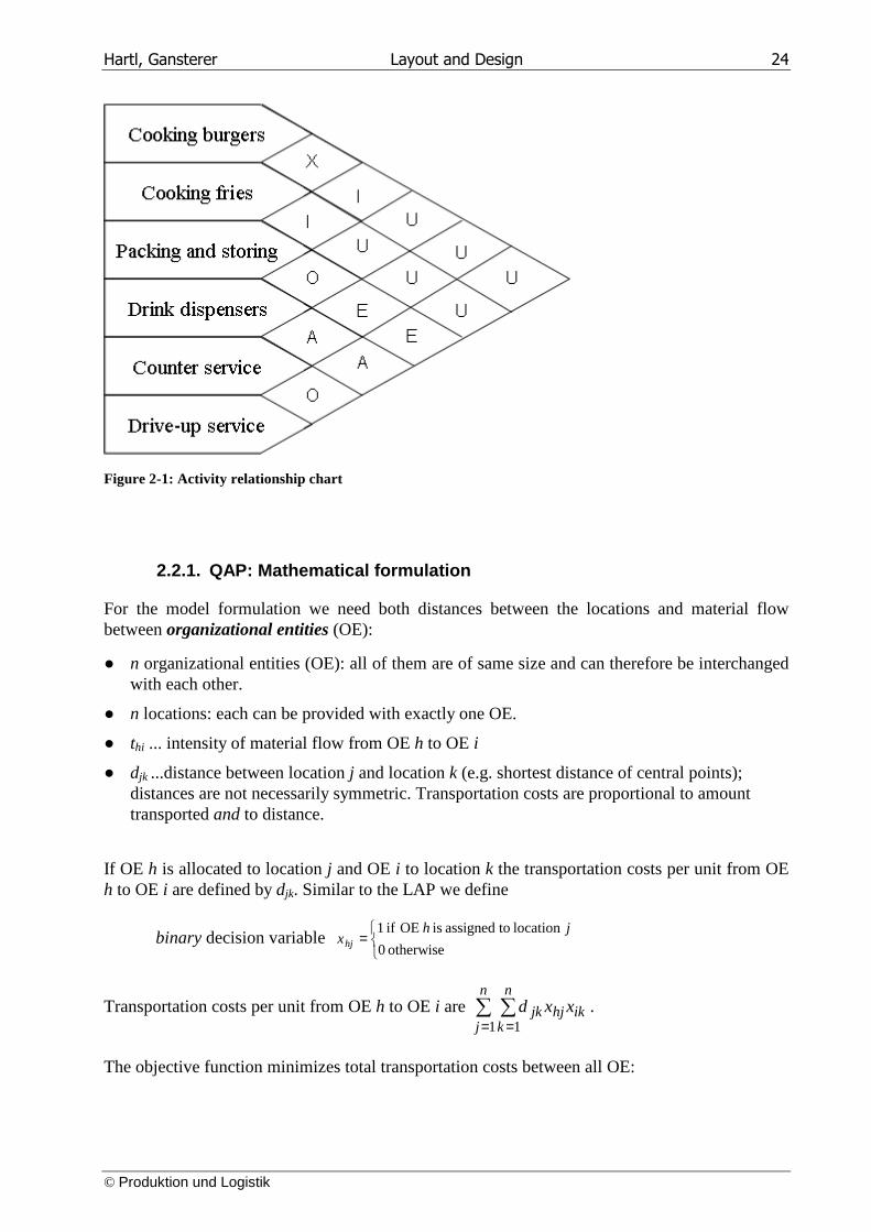
The burgers are cooked on a large grill, and the fries are deep fried in hot oil. For safety reasons the company requires that these cooking areas not be located near each other. All hamburgers are individually wrapped after cooking and stored near the counter. The service counter can accommodate six servers, and the site has an area reserved for a drive-up window.
An activity relationship chart for this facility appears in the following. In the chart, each pair of activities is given one of the letter designations A, E, I, O, U, or X. Once a final layout is determined, the proximity of the various departments can be compared to the closeness ratings in the chart. Figure 2-1 illustrates the activity relationship chart for Met me Inc .”8
In the original conception of the QAP a number giving the reason for each closeness rating is needed as well. In case of closeness rating “X” a negative value would be used to indicate the undesirability of closeness for the according machines/operations.
Hartl, Gansterer Layout and Design 24
© Produktion und Logistik
2.2.1. QAP: Mathematical formulation
For the model formulation we need both distances between the locations and material flow between organizational entities (OE):
● n organizational entities (OE): all of them are of same size and can therefore be interchanged with each other.
● n locations: each can be provided with exactly one OE.
● thi ... intensity of material flow from OE h to OE i
● djk ...distance between location j and location k (e.g. shortest distance of central points); distances are not necessarily symmetric. Transportation costs are proportional to amount transported and to distance.
If OE h is allocated to location j and OE i to location k the transportation costs per unit from OE h to OE i are defined by djk. Similar to the LAP we define
binary decision variable
=otherwise 0
location toassigned is OE if 1 jhxhj
Transportation costs per unit from OE h to OE i are ∑ ∑= =
n
j
n
kikhjjk xxd
1 1.
The objective function minimizes total transportation costs between all OE:
Figure 2-1: Activity relationship chart
Hartl, Gansterer Layout and Design 25
© Produktion und Logistik
min1 1 1 1
→∑ ∑ ∑ ∑= = = =
n
h
n
i
n
j
n
kikhjjkhi xxdt
where we refer to the following constraints (similar to the LAP):
11
=∑=
n
jhjx for h = 1, ... , n ... each OE h on exactly 1 location j
11
=∑=
n
hhjx for j = 1, ... , n ... each location j gets exactly 1 OE h
hjx = 0 or 1 ... binary decision variable
While all constraints are still linear we now face a non-linear objective function. Due to the combination of integer property and non-linearity finding optimal solutions for larger problems is almost impossible (cf. Fehler! Verweisquelle konnte nicht gefunden werden.). Thus, heuristic methods are applied in most cases. As usual we distinguish between starting heuristics and improvement methods or a combination of both of them.
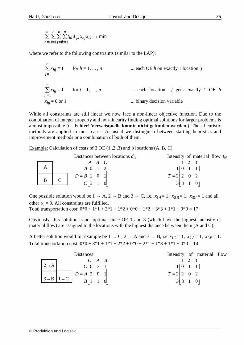
Example: Calculation of costs of 3 OE (1 ,2 ,3) and 3 locations (A, B, C)
A
B C
Distances between locations djk
=013
101
210
C
B
A
D
CBA
Intensity of material flow thi
=013
202
110
3
2
1321
T
One possible solution would be 1 → A, 2 → B and 3 → C, i.e. Ax1 = 1, Bx2 = 1, Cx3 = 1 and all
other thj = 0. All constraints are fulfilled. Total transportation cost: 0*0 + 1*1 + 2*1 + 1*2 + 0*0 + 1*2 + 3*3 + 1*1 + 0*0 = 17
Obviously, this solution is not optimal since OE 1 and 3 (which have the highest intensity of material flow) are assigned to the locations with the highest distance between them (A and C).
A better solution would for example be 1 → C, 2 → A and 3 → B, i.e. Cx1 = 1, Ax2 = 1, Bx3 = 1.
Total transportation cost: 0*0 + 3*1 + 1*1 + 2*2 + 0*0 + 2*1 + 1*3 + 1*1 + 0*0 = 14
2→A
3→B 1→C
Distances
=011
102
130
B
A
C
D
BAC
Intensity of material flow
=013
202
110
3
2
1321
T
Hartl, Gansterer Layout and Design 26
© Produktion und Logistik
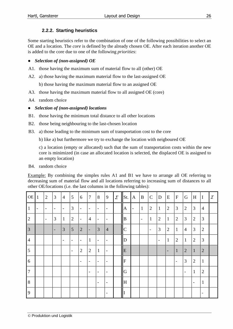
2.2.2. Starting heuristics
Some starting heuristics refer to the combination of one of the following possibilities to select an OE and a location. The core is defined by the already chosen OE. After each iteration another OE is added to the core due to one of the following priorities:
● Selection of (non-assigned) OE
A1. those having the maximum sum of material flow to all (other) OE
A2. a) those having the maximum material flow to the last-assigned OE
b) those having the maximum material flow to an assigned OE
A3. those having the maximum material flow to all assigned OE (core)
A4. random choice
● Selection of (non-assigned) locations
B1. those having the minimum total distance to all other locations
B2. those being neighbouring to the last-chosen location
B3. a) those leading to the minimum sum of transportation cost to the core
b) like a) but furthermore we try to exchange the location with neigboured OE
c) a location (empty or allocated) such that the sum of transportation costs within the new core is minimized (in case an allocated location is selected, the displaced OE is assigned to an empty location)
B4. random choice
Example: By combining the simples rules A1 and B1 we have to arrange all OE referring to decreasing sum of material flow and all locations referring to increasing sum of distances to all other OE/locations (i.e. the last columns in the following tables):
OE 1 2 3 4 5 6 7 8 9 Σ St. A B C D E F G H I Σ
1 - - - - 3 - - - - A - 1 2 1 2 3 2 3 4
2 - 3 1 2 - 4 - - B - 1 2 1 2 3 2 3
3 - 3 5 2 - 3 4 C - 3 2 1 4 3 2
4 - - - 1 - - D - 1 2 1 2 3
5 - 2 2 1 - E - 1 2 1 2
6 - - - - F - 3 2 1
7 - - - G - 1 2
8 - - H - 1
9 - I -
Hartl, Gansterer Layout and Design 27
© Produktion und Logistik
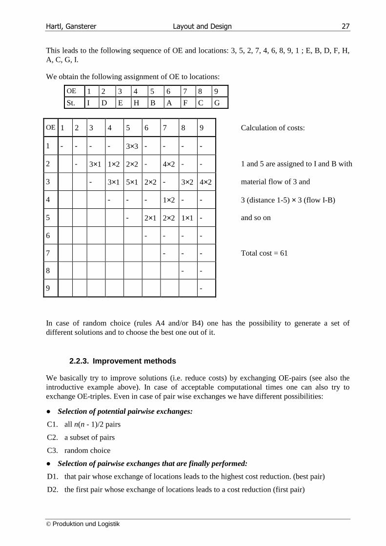
This leads to the following sequence of OE and locations: 3, 5, 2, 7, 4, 6, 8, 9, 1 ; E, B, D, F, H, A, C, G, I.
We obtain the following assignment of OE to locations:
OE 1 2 3 4 5 6 7 8 9
St. I D E H B A F C G
OE 1 2 3 4 5 6 7 8 9 Calculation of costs:
1 - - - - 3×3 - - - -
2 - 3×1 1×2 2×2 - 4×2 - - 1 and 5 are assigned to I and B with
3 - 3×1 5×1 2×2 - 3×2 4×2 material flow of 3 and
4 - - - 1×2 - - 3 (distance 1-5) × 3 (flow I-B)
5 - 2×1 2×2 1×1 - and so on
6 - - - -
7 - - - Total cost = 61
8 - -
9 -
In case of random choice (rules A4 and/or B4) one has the possibility to generate a set of different solutions and to choose the best one out of it.
2.2.3. Improvement methods
We basically try to improve solutions (i.e. reduce costs) by exchanging OE-pairs (see also the introductive example above). In case of acceptable computational times one can also try to exchange OE-triples. Even in case of pair wise exchanges we have different possibilities:
● Selection of potential pairwise exchanges:
C1. all n(n - 1)/2 pairs
C2. a subset of pairs
C3. random choice
● Selection of pairwise exchanges that are finally performed:
D1. that pair whose exchange of locations leads to the highest cost reduction. (best pair)
D2. the first pair whose exchange of locations leads to a cost reduction (first pair)
Hartl, Gansterer Layout and Design 28
© Produktion und Logistik
A combination of C1 and D1 increases solution quality but also computational time. A common method is to start with C2 and skip to C1 as soon as the solution is reasonably good. (A combination of C1 and D2 is equivalent to the 2-opt method which we use to solve TSP).
A well-known (heuristic) method is CRAFT (computerized relative allocation of facilities techniques) which equals (in case of OE with similar place requirements) a combination of C1 and D1 (this method will be introduced later in this chapter in the context of OE with unequal place requirements).
In case of random choice (C3 and D2) we quite often find good results. Especially the fact that sometimes the best exchange of all exchanges which have been checked leads to an increase of costs is no disadvantage, because it reduces the risk to be trapped in local optima.
The basic idea and several adaptions/combinations of A, B, C, and D are discussed in literature.
2.2.4. „Umlaufmethode“
„Umlaufmethode“ is one of the numerous heuristics which combine the idea of starting heuristics and imporvement methods. This method consists of the following components:
Initialization ( i = 1): Those OE having the maximum sum of material flow [A1] is assigned to the centre of locations (i.e. the location having the minimum sum of distances to all other locations [B1]).
Iteration i ( i = 2, ... , n): assign OE i
Part 1: (Selection of OE and of free location):
● select those OE with the maximum sum of material flow to all OE assigned to the core [A3]
● assign the selected OE to a free location so that the sum of transportation costs to the core (within the core) is minimized [B3a]
Part 2: (Improvement step in iteration i = 4):
● check pair wise exchanges of the last-assigned OE with all other OE in the core [C2]
● if an improvement is found, the exchange is conducted and we start again with Part 2 [D2].
The method ends with the finalization of iteration i = n having assigned all OE.
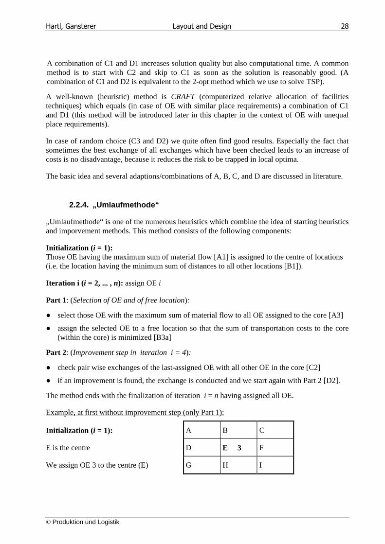
Example, at first without improvement step (only Part 1):
Initialization ( i = 1): A B C
E is the centre D E 3 F
We assign OE 3 to the centre (E) G H I
Hartl, Gansterer Layout and Design 29
© Produktion und Logistik
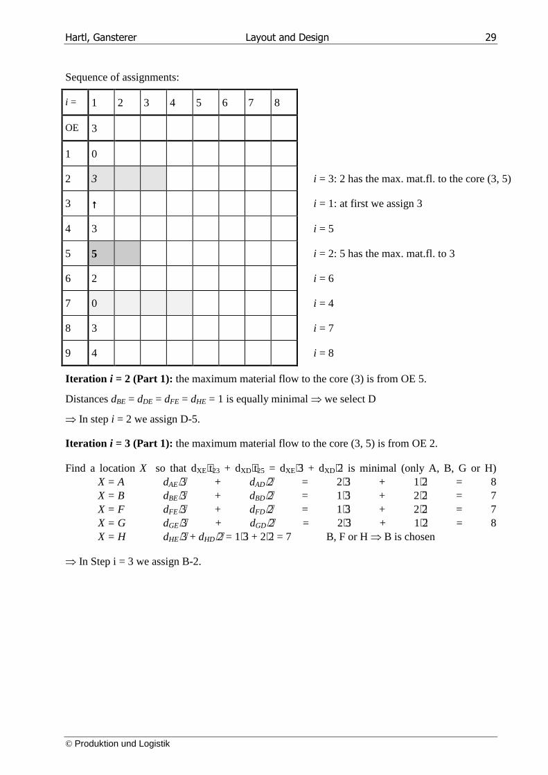
Sequence of assignments:
i = 1 2 3 4 5 6 7 8
OE 3
1 0
2 3 i = 3: 2 has the max. mat.fl. to the core (3, 5)
3 ↑↑↑↑ i = 1: at first we assign 3
4 3 i = 5
5 5 i = 2: 5 has the max. mat.fl. to 3
6 2 i = 6
7 0 i = 4
8 3 i = 7
9 4 i = 8
Iteration i = 2 (Part 1): the maximum material flow to the core (3) is from OE 5.
Distances dBE = dDE = dFE = dHE = 1 is equally minimal ⇒ we select D
⇒ In step i = 2 we assign D-5.
Iteration i = 3 (Part 1): the maximum material flow to the core (3, 5) is from OE 2.
Find a location X so that dXE⋅t23 + dXD⋅t25 = dXE⋅3 + dXD⋅2 is minimal (only A, B, G or H) X = A dAE⋅3 + dAD⋅2 = 2⋅3 + 1⋅2 = 8 X = B dBE⋅3 + dBD⋅2 = 1⋅3 + 2⋅2 = 7 X = F dFE⋅3 + dFD⋅2 = 1⋅3 + 2⋅2 = 7 X = G dGE⋅3 + dGD⋅2 = 2⋅3 + 1⋅2 = 8 X = H dHE⋅3 + dHD⋅2 = 1⋅3 + 2⋅2 = 7 B, F or H ⇒ B is chosen
⇒ In Step i = 3 we assign B-2.
Hartl, Gansterer Layout and Design 30
© Produktion und Logistik
Iteration i = 4 (Part 1) the maximum material flow to the core (2, 3, 5) is from OE 7.
Find a location X so that dXE⋅t73 + dXD⋅t75 + dXB⋅t72 = dXE⋅0 + dXD⋅2 + dXB⋅4 is minimal in the map we see that A is the best choice ⇒ in iteration i = 4 we tentatively assign A-7.
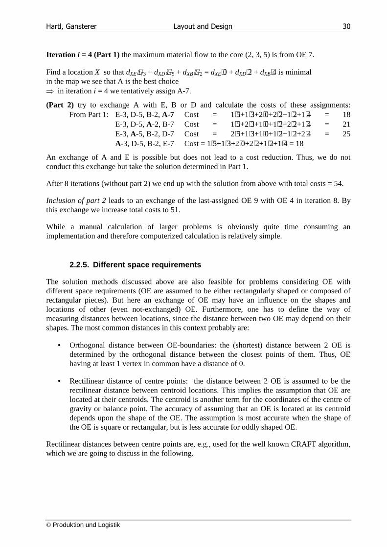
(Part 2) try to exchange A with E, B or D and calculate the costs of these assignments: From Part 1: E-3, D-5, B-2, A-7 Cost = 1⋅5+1⋅3+2⋅0+2⋅2+1⋅2+1⋅4 = 18 E-3, D-5, A-2, B-7 Cost = 1⋅5+2⋅3+1⋅0+1⋅2+2⋅2+1⋅4 = 21 E-3, A-5, B-2, D-7 Cost = 2⋅5+1⋅3+1⋅0+1⋅2+1⋅2+2⋅4 = 25 A-3, D-5, B-2, E-7 Cost = 1⋅5+1⋅3+2⋅0+2⋅2+1⋅2+1⋅4 = 18
An exchange of A and E is possible but does not lead to a cost reduction. Thus, we do not conduct this exchange but take the solution determined in Part 1.
After 8 iterations (without part 2) we end up with the solution from above with total costs = 54.
Inclusion of part 2 leads to an exchange of the last-assigned OE 9 with OE 4 in iteration 8. By this exchange we increase total costs to 51.
While a manual calculation of larger problems is obviously quite time consuming an implementation and therefore computerized calculation is relatively simple.
2.2.5. Different space requirements
The solution methods discussed above are also feasible for problems considering OE with different space requirements (OE are assumed to be either rectangularly shaped or composed of rectangular pieces). But here an exchange of OE may have an influence on the shapes and locations of other (even not-exchanged) OE. Furthermore, one has to define the way of measuring distances between locations, since the distance between two OE may depend on their shapes. The most common distances in this context probably are:
• Orthogonal distance between OE-boundaries: the (shortest) distance between 2 OE is determined by the orthogonal distance between the closest points of them. Thus, OE having at least 1 vertex in common have a distance of 0.
• Rectilinear distance of centre points: the distance between 2 OE is assumed to be the rectilinear distance between centroid locations. This implies the assumption that OE are located at their centroids. The centroid is another term for the coordinates of the centre of gravity or balance point. The accuracy of assuming that an OE is located at its centroid depends upon the shape of the OE. The assumption is most accurate when the shape of the OE is square or rectangular, but is less accurate for oddly shaped OE.
Rectilinear distances between centre points are, e.g., used for the well known CRAFT algorithm, which we are going to discuss in the following.
Hartl, Gansterer Layout and Design 31
© Produktion und Logistik
2.2.5.1. CRAFT Algorithm 910
CRAFT (computerized relative allocation of facilities techniques) was one of the first computer-aided layout routines developed. It is an improvement method which means that it requires an initial layout to be used as a starting solution.
Again we try to improve the given solution by moving around OE. The additional challenge now is that the shapes of OE are not fixed. Thus, the problem simply has too many degrees of freedom for us to devise a good method for modifying the starting solution. All the common improvement methods are based on limiting the kinds of changes that are permitted. This has already been addressed in the context of problems with similar space requirements.
We know that a pair of OE that can be exchanged without a direct influence on the shapes or locations of all remaining OE has to satisfy one of the following conditions:
1. the OE have the same space requirement,
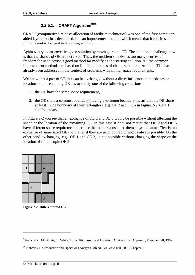
2. the OE share a common boundary (having a common boundary means that the OE share at least 1 side boundary of their rectangles). E.g. OE 2 and OE 5 in Figure 2-2 share 1 side boundary.
In Figure 2-2 you see that an exchange of OE 2 and OE 5 would be possible without affecting the shape or the location of the remaining OE. In this case it does not matter that OE 2 and OE 5 have different space requirements because the total area used for them stays the same. Clearly, an exchange of same sized OE (no matter if they are neighboured or not) is always possible. On the other hand exchanging, e.g., OE 1 and OE 3, is not possible without changing the shape or the location of for example OE 2.
1 4
2 5
3
Figure 2-2: Different sized OE
9 Francis, R., McGinnis, L., White, J., Facility Layout and Location: An Analytical Approach, Prentice Hall, 1992
10 Nahmias, S.: Production and Operations Analysis, 4th ed., McGraw-Hill, 2000, Chapter 10
Hartl, Gansterer Layout and Design 32
© Produktion und Logistik
The CRAFT algorithm, which is probably the earliest widely known improvement algorithm, uses an estimate of the transportation cost that is based on the rectilinear distance between the centroid locations. If, e.g., OE 2 and 5 are considered for an exchange, the new costs is estimated by assuming that the new centroid of OE 2 is the old centroid of OE 5 and vice versa. This method of estimating transportation costs for the new layout is exact if OE have the same space requirement, but can be in error if the requirements are different. In this case we revise the estimated transportation costs by developing a distance chart for the new layout and calculating the “real” total transportation costs. This is done whenever an exchange has been identified to be the most useful (based on the estimation of costs) in an iteration. The algorithm continues until no further reductions in the predicted transportation costs can be achieved.
So we summarize the steps to be followed according to CRAFT:
1. Estimate total transportation costs considering all pairwise exchanges of OE that share at least 1 border or that are of same size (i.e. equal number of rectangles).
2. Perform that exchange that leads to the minimum estimated total transportation costs (based on an estimation of distances as described above). If all possible exchanges lead to an increase of predicted total costs, stop here.
3. Revise the estimated distance chart and calculate the new total costs. Go back to step 1.
You see that by applying this procedure the “best” exchange could be passed over, due to estimation errors. This generally will be the case for any improvement algorithm that does not actually evaluate every exchange possible.
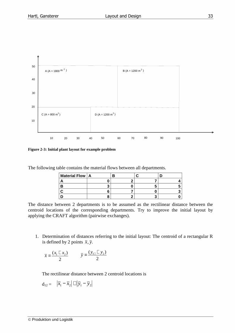
Example11: A local manufacturing firm has recently completed construction of a new plant to house 4 departments: A, B, C, and D. The plant is 100m2 by 50m2. The plant manager has chosen an initial layout of the 4 departments. This layout is given in Figure 2-3. From the figure we see that department A requires 1800 m2, department B 1200m2, department C 800m2, and department D 1200m2.
11 Nahmias, S.: Production and Operations Analysis, 4th ed., McGraw-Hill, 2000, Chapter 10
Hartl, Gansterer Layout and Design 33
© Produktion und Logistik
The following table contains the material flows between all departments.
Material Flow A B C D A 0 2 7 4 B 3 0 5 5 C 6 7 0 3 D 8 2 3 0
The distance between 2 departments is to be assumed as the rectilinear distance between the centroid locations of the corresponding departments. Try to improve the initial layout by applying the CRAFT algorithm (pairwise exchanges).
1. Determination of distances referring to the initial layout: The centroid of a rectangular R is defined by 2 points ., yx
The rectilinear distance between 2 centroid locations is
d12 =
Figure 2-3: Initial plant layout for example problem
2
)( 21 xxx
+=2
)( 21 yyy
+= +
2121 yyxx −+−
10 30 40 50 60 70 80 90 100
20
30
40
50 A (A = 1800 m 2 ) B (A = 1200 m 2 )
C (A = 800 m2 ) D (A = 1200 m2 )
10
20
Hartl, Gansterer Layout and Design 34
© Produktion und Logistik
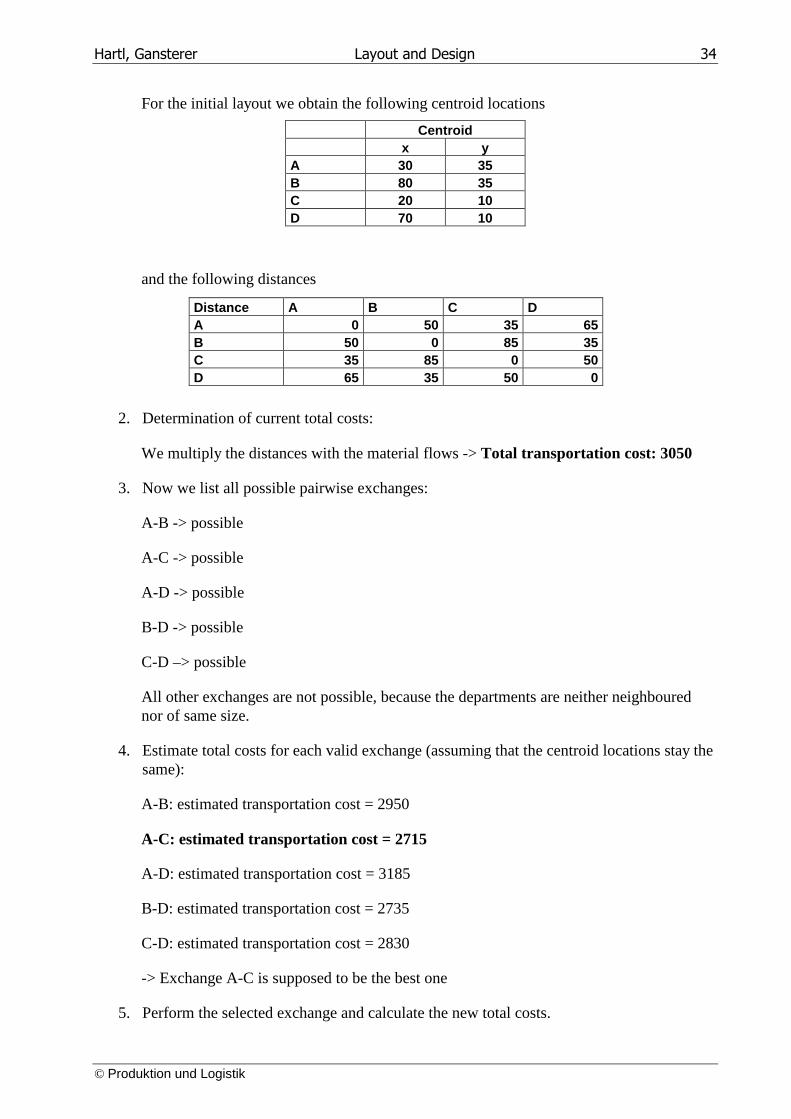
For the initial layout we obtain the following centroid locations
Centroid x y A 30 35 B 80 35 C 20 10 D 70 10
and the following distances
2. Determination of current total costs:
We multiply the distances with the material flows -> Total transportation cost: 3050
3. Now we list all possible pairwise exchanges:
A-B -> possible
A-C -> possible
A-D -> possible
B-D -> possible
C-D –> possible
All other exchanges are not possible, because the departments are neither neighboured nor of same size.
4. Estimate total costs for each valid exchange (assuming that the centroid locations stay the same):
A-B: estimated transportation cost = 2950
A-C: estimated transportation cost = 2715
A-D: estimated transportation cost = 3185
B-D: estimated transportation cost = 2735
C-D: estimated transportation cost = 2830
-> Exchange A-C is supposed to be the best one
5. Perform the selected exchange and calculate the new total costs.
Distance A B C D A 0 50 35 65 B 50 0 85 35 C 35 85 0 50 D 65 35 50 0
Hartl, Gansterer Layout and Design 35
© Produktion und Logistik
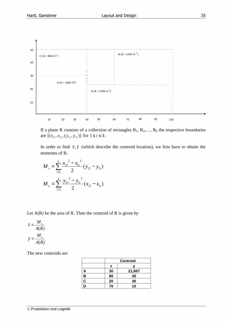
If a plane R consists of a collection of rectangles R1, R2,…, Rk the respective boundaries are )],(,,[( 2121 iiii yyxx for .1 ki ≤≤
In order to find yx, (which describe the centroid location), we first have to obtain the moments of R:
Let A(R) be the area of R. Then the centroid of R is given by
The new centroids are
Centroid x y A 30 21,667 B 80 35 C 20 40 D 70 10
∑=
−−=k
iii
iix yy
xxM
112
21
22 )(
2
∑=
−−=k
iii
iiy xx
yyM
112
21
22 )(
2
)(
)(
RA
My
RA
Mx
y
x
=
=
10 30 40 50 60 70 80 90 100
20
30
40
50
A (A = 1800 m2)
B (A = 1200 m 2 )C (A = 800 m2 )
D (A = 1200 m 2)
10
20
Hartl, Gansterer Layout and Design 36
© Produktion und Logistik
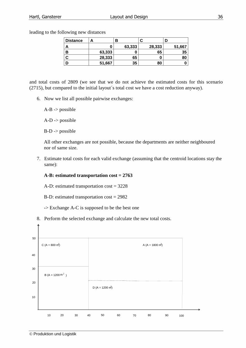
leading to the following new distances
Distance A B C D A 0 63,333 28,333 51,667 B 63,333 0 65 35 C 28,333 65 0 80 D 51,667 35 80 0
and total costs of 2809 (we see that we do not achieve the estimated costs for this scenario (2715), but compared to the initial layout´s total cost we have a cost reduction anyway).
6. Now we list all possible pairwise exchanges:
A-B -> possible
A-D -> possible
B-D -> possible
All other exchanges are not possible, because the departments are neither neighboured nor of same size.
7. Estimate total costs for each valid exchange (assuming that the centroid locations stay the same):
A-B: estimated transportation cost = 2763
A-D: estimated transportation cost = 3228
B-D: estimated transportation cost = 2982
-> Exchange A-C is supposed to be the best one
8. Perform the selected exchange and calculate the new total costs.
20 30 40 50 60 70 80 90 100
20
30
40
50
B (A = 1200 m 2)
A (A = 1800 m2)C (A = 800 m2)
D (A = 1200 m2)
10
10
Hartl, Gansterer Layout and Design 37
© Produktion und Logistik
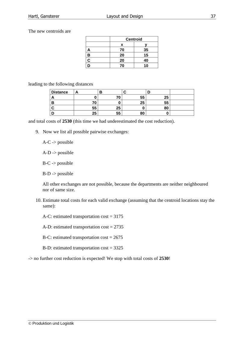
The new centroids are
Centroid x y A 70 35 B 20 15 C 20 40 D 70 10
leading to the following distances
Distance A B C D A 0 70 55 25 B 70 0 25 55 C 55 25 0 80 D 25 55 80 0
and total costs of 2530 (this time we had underestimated the cost reduction).
9. Now we list all possible pairwise exchanges:
A-C -> possible
A-D -> possible
B-C -> possible
B-D -> possible
All other exchanges are not possible, because the departments are neither neighboured nor of same size.
10. Estimate total costs for each valid exchange (assuming that the centroid locations stay the same):
A-C: estimated transportation cost = 3175
A-D: estimated transportation cost = 2735
B-C: estimated transportation cost = 2675
B-D: estimated transportation cost = 3325
-> no further cost reduction is expected! We stop with total costs of 2530!
Hartl, Gansterer Layout and Design 38
© Produktion und Logistik
3. Group Technology / Cellular Manufacturing 12
3.1 Introduction
As early as in the 1920ies it was observed, that using product-oriented departments to manufacture standardized products in machine companies lead to reduced transportation. This can be considered the start of Group Technology (GT). Parts are classified and parts with similar features are manufactured together with standardized processes. As a consequence, small "focused factories" are being created as independent operating units within large facilities.
More generally, Group Technology can be considered a theory of management based on the principle that "similar things should be done similarly". In our context, "things" include product design, process planning, fabrication, assembly, and production control. However, in a more general sense GT may be applied to all activities, including administrative functions.
The principle of group technology is to divide the manufacturing facility into small groups or cells of machines. The term cellular manufacturing is often used in this regard. Each of these cells is dedicated to a specified family or set of part types. Typically, a cell is a small group of machines (as a rule of thumb not more than five). An example would be a machining center with inspection and monitoring devices, tool and Part Storage, a robot for part handling, and the associated control hardware.
The idea of GT can also be used to build larger groups, such as for instance, a department, possibly composed of several automated cells or several manned machines of various types. As mentioned in Chapter 1 (see also Figure 1.5) pure item flow lines are possible, if volumes are very large. If volumes are very small, and parts are very different, a functional layout (job shop) is usually appropriate. In the intermediate case of medium-variety, medium-volume environments, group configuration is most appropriate.
GT can produce considerable improvements where it is appropriate and the basic idea can be utilized in all manufacturing environments:
• To the manufacturing engineer GT can be viewed as a role model to obtain the advantages of flow line systems in environments previously ruled by job shop layouts. The idea is to form groups and to aim at a product-type layout within each group (for a family of parts). Whenever possible, new parts are designed to be compatible with the processes and tooling of an existing part family. This way, production experience is quickly obtained, and standard process plans and tooling can be developed for this restricted part set.
• To the design engineer the idea of GT can mean to standardize products and process plans. If a new part should be designed, first retrieve the design for a similar, existing part. Maybe, the need for the new part is eliminated if an existing part will suffice. If a
12 This chapter is based on Chapter 6 of Askin & Standridge (1993). It is recommended to read this chapter parallel to the course notes.
Hartl, Gansterer Layout and Design 39
© Produktion und Logistik
new part is actually needed, the new plan can be developed quickly by relying on decisions and documentation previously made for similar parts. Hence, the resulting plan will match current manufacturing procedures and document preparation time is reduced. The design engineer is freed to concentrate on optimal design.
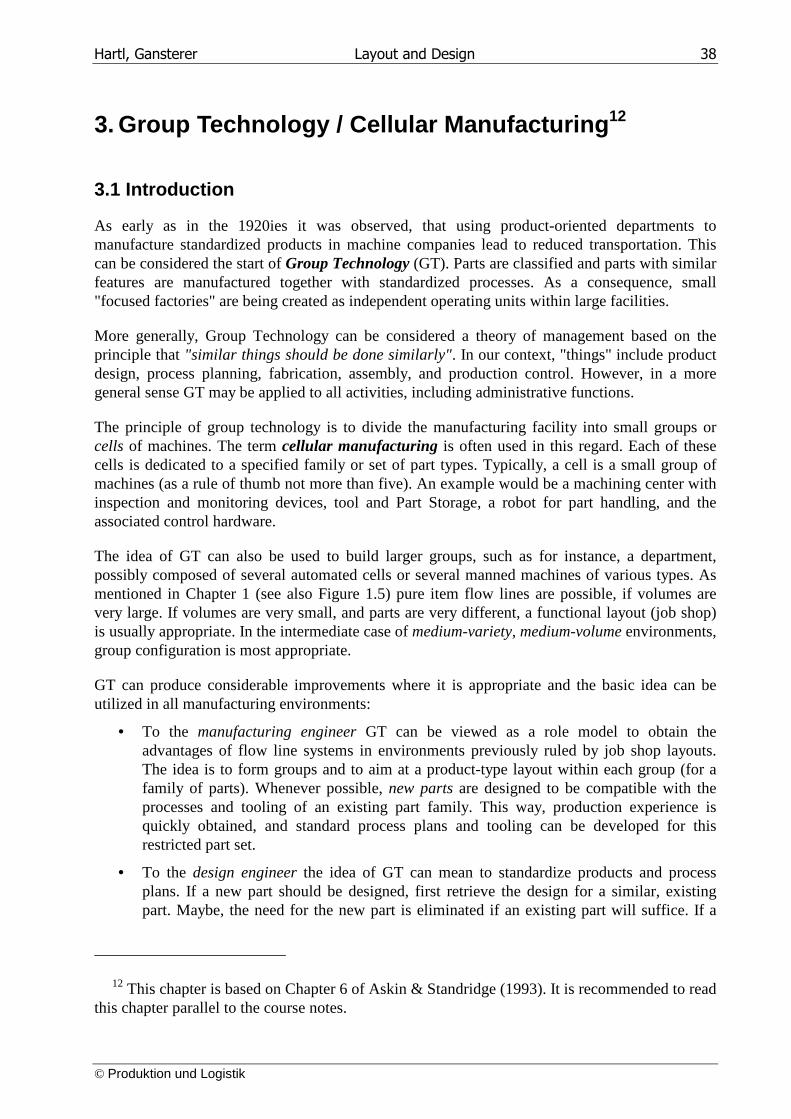
In this GT context a typical approach would be the use of composite Part families. Consider e.g. the parts family shown in Figure 3.1.
Figure 3.1. Composite Group Technology Part (Askin & Standridge, 1993, p. 165).
The parameter values for the features of this single part family have the same allowable ranges. Each part in the family requires the same set of machines and tools; in our example: turning/lathing (Drehbank), internal drilling (Bohrmaschine), face milling (Planfräsen), etc.
Raw material should be reasonably consistent (e.g. plastic and metallic parts require different manufacturing operations and should not be in the same family).
Fixtures can be designed that are capable of supporting all the actual realizations of the composite parts within the family.
Standard machine setups are often possible with little or no changeover required between the different parts within the family (same material, same fixture method, similar size, same tools/machines required).
In the functional process (job shop) layout, all parts travel through the entire shop. Scheduling and material control are complicated. Job priorities are difficult to set, and large WIP inventories are used to assure reasonable capacity utilisation. In GT, each part type flows only through its specific group area. The reduced setup time allows faster adjustment to changing conditions.
Often, workers are cross-trained on all machines within the group and follow the job from Start to finish. This usually leads to higher job satisfaction/motivation and higher efficiency.
For smaller-volume part families it may be necessary to include several such part families in a machine group to justify machine utilization.
One can identify three different types group layout:
Hartl, Gansterer Layout and Design 40
© Produktion und Logistik
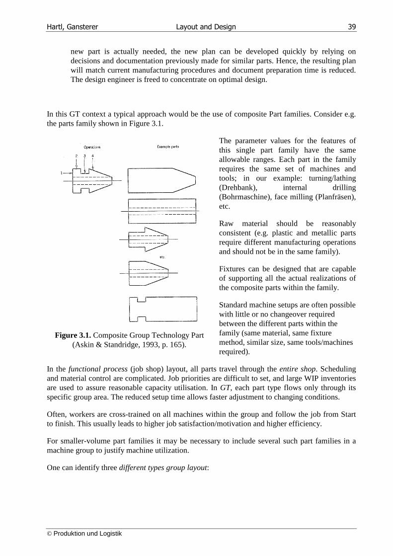
Figure 3.2a. GT flow line (Askin & Standridge, 1993, p. 167).
In a GT flow line concept all parts assigned to a group follow the same machine sequence and require relatively proportional time requirements on each machine.
The GT flow line operates as a mixed-product assembly line system; see Figure 3.2a. Automated transfer mechanisms may be possible. See also Chapter 4 for mixed-product assembly lines.
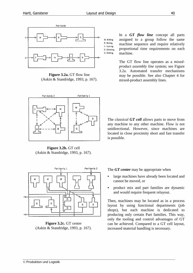
Figure 3.2b. GT cell (Askin & Standridge, 1993, p. 167).
The classical GT cell allows parts to move from any machine to any other machine. Flow is not unidirectional. However, since machines are located in close proximity short and fast transfer is possible.
Figure 3.2c. GT center (Askin & Standridge, 1993, p. 167).
The GT center may be appropriate when
• large machines have already been located and cannot be moved, or
• product mix and part families are dynamic and would require frequent relayout.
Then, machines may be located as in a process layout by using functional departments (job shops), but each machine is dedicated to producing only certain Part families. This way, only the tooling and control advantages of GT can be achieved. Compared to a GT cell layout, increased material handling is necessary.
Hartl, Gansterer Layout and Design 41
© Produktion und Logistik
GT offers numerous benefits w.r.t. throughput time, WIP inventory, materials handling, job satisfaction, fixtures, setup time, space needs, quality, finished goods, and labor cost; read also Chapter 6.1 of Askin & Standridge, 1993.
In general, GT simplifies and standardizes. The approach to simplify, standardize, and internalize through repetition produces efficiency.
Since a workcenter will work only on a family of similar parts generic fixtures can be developed and used. Tooling can be stored locally since parts will always be processed through the same machines. Tool changes may be required due to tool wear only, not part changeovers (e.g. a press may have a generic fixture that can hold all the parts in a family without any change or simply by changing a part-specific insert secured by a single screw. Hence setup time is reduced, and tooling cost is reduced. Using queuing theory (M/M/1 model) it is possible to show that if setup time is reduced, also the throughput time for the system is reduced by the same percentage.
3.2 How to form groups
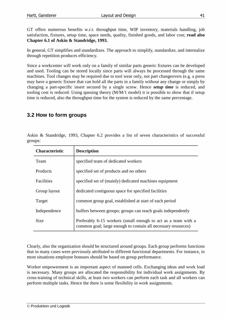
Askin & Standridge, 1993, Chapter 6.2 provides a list of seven characteristics of successful groups:
Characteristic Description
Team specified team of dedicated workers
Products specified set of products and no others
Facilities specified set of (mainly) dedicated machines equipment
Group layout dedicated contiguous space for specified facilities
Target common group goal, established at start of each period
Independence buffers between groups; groups can reach goals independently
Size Preferably 6-15 workers (small enough to act as a team with a common goal; large enough to contain all necessary resources)
Clearly, also the organization should be structured around groups. Each group performs functions that in many cases were previously attributed to different functional departments. For instance, in most situations employee bonuses should be based on group performance.
Worker empowerment is an important aspect of manned cells. Exchanging ideas and work load is necessary. Many groups are allocated the responsibility for individual work assignments. By cross-training of technical skills, at least two workers can perform each task and all workers can perform multiple tasks. Hence the there is some flexibility in work assignments.
Hartl, Gansterer Layout and Design 42
© Produktion und Logistik
The group should be an independent profit center in some sense. It should also retain the responsibility for its performance and authority to affect that performance. The group is a single entity and must act together to resolve problems.
There are three basic steps in group technology planning:
1. coding 2. classification 3. layout.
These will be discussed in separate subsections.
3.3 Coding schemes
The knowledge concerning the similarities between parts must be coded somehow. This will facilitate determination and retrieval of similar parts. Often this involves the assignment of a symbolic or numerical description to parts (part number) based on their design and manufacturing characteristics. However, it may also simply mean listing the machines used by each part.
There are four major issues in the construction of a coding system:
• part (component) population • code detail • code structure, and • (digital) representation.
Numerous codes exist, including Brisch-Birn, MULTICLASS, and KK-3. One of the most widely used coding systems is OPITZ. Many firms customize existing coding systems to their specific needs. Important aspects are
• The code should be sufficiently flexible to handle future as well as current parts. • The scope of part types to be included must be known (e.g. are the parts rotational,
prismatic, sheet metal, etc.?) • To be useful, the code must discriminate between parts with different values for key
attributes (material, tolerances, required machines, etc.)
Code detail is crucial to the success of the coding project. Ideal is a short code that uniquely identifies each part and fully describes the part from design and manufacturing viewpoints,
• Too much detail results in cumbersome codes and the waste of resources in data collection.
• With too few details and the code becomes useless.
As a general rule, all information necessary for grouping the part for manufacturing should be included in the code whenever possible. Features like outside shape, end shape, internal shape, holes, and dimensions are typically included in the coding scheme.
Hartl, Gansterer Layout and Design 43
© Produktion und Logistik
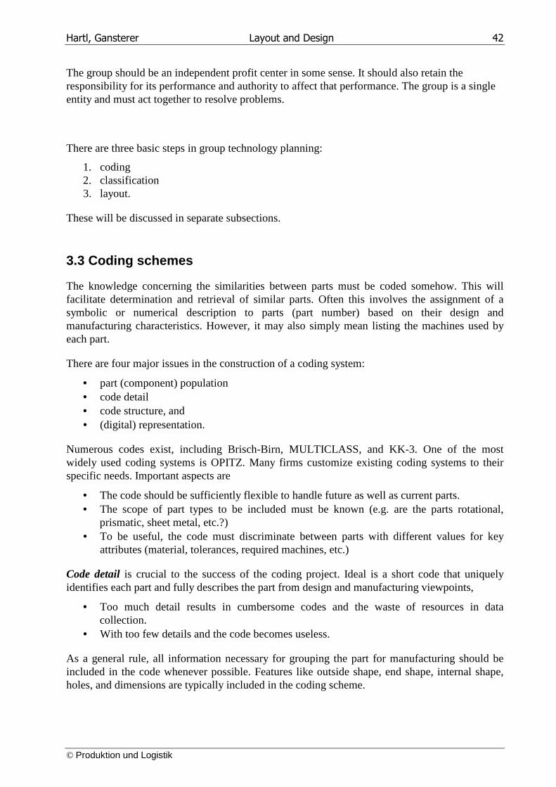
W.r.t. code structure, codes are generally classified as, hierarchical (also called monocode), chain (also called polycode), or hybrid. This is explained in Figure 3.3 (taken from Askin & Standridge, 1993).
Figure 3.3a. Hierarchical structure.
Hierarchical code structure: the meaning of a digit in the code depends on the values of preceding digits. The value of 3 in the third place may indicate
• the existence of internal threads in a rotational part: "1232"
• a smooth internal feature: "2132"
Hierarchical codes are efficient; they only consider relevant information at each digit. But they are difficult to learn because of the large number of conditional inferences.
Figure 3.3b. Chain structure.
Chain code: each value for each digit of the code has a consistent meaning. The value 3 in the third place has the same meaning for all parts.
They are easier to learn but less efficient. Certain digits may be almost meaningless for some parts.
Figure 3.3c. Chain structure.
Since both hierarchical and chain codes have advantages, many commercial codes are hybrid: combination of both:
Some section of the code is a chain code and then several hierarchical digits further detail the specified characteristics. Several such sections may exist. One example of a hybrid code is OPITZ.
The final decision is, code representation. The digits can be
• numeric or even binary; for direct use in computer (storage and retrieval efficiency)
• alphabetic; humans are more comfortable with a coding like "S" for smooth or "T" for thread (Gewinde) than with digits
The proper decision process involves the design engineer, manufacturing engineer, and Computer scientist working together as a team.
A well known coding system is OPITZ. It can have 3 sections:
Hartl, Gansterer Layout and Design 44
© Produktion und Logistik
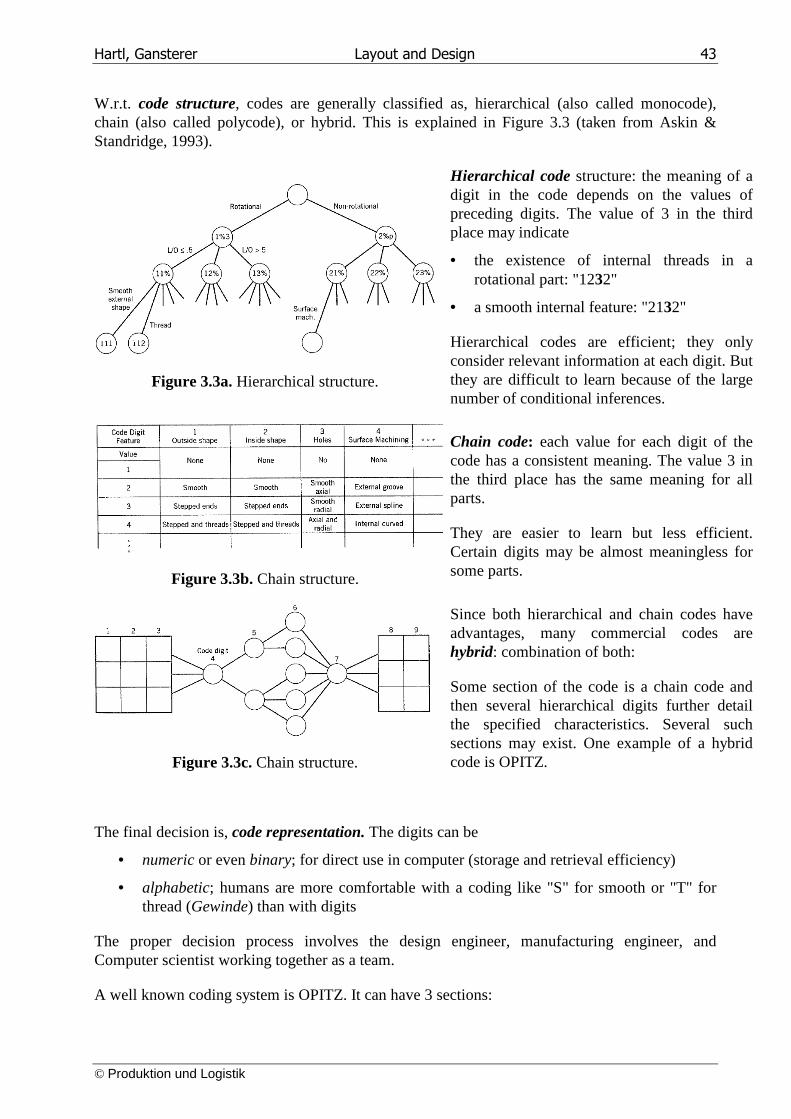
• it starts with a five-digit "geometric form code" • followed by a fourdigit "supplementary code." • This may be followed by a company-specific four-digit "secondary code" intended for
describing production operations and sequencing.
Figure 3.4. Overview of the Opitz code (Askin & Standridge, 1993, p. 167).
Digit 1: shows whether the part is rotational and also the basic dimension ratio (length/diameter if rotational, length/width if nonrotational).
Digit 2: main external shape; partly dependent on digit 1.
Digit 3: main internal shape.
Digit 4: machining requirements for plane surfaces.
Digit 5: auxiliary features like additional holes, etc.
For more details on the meaning of these digits see Figure 6.6 in Askin & Standridge, 1993.
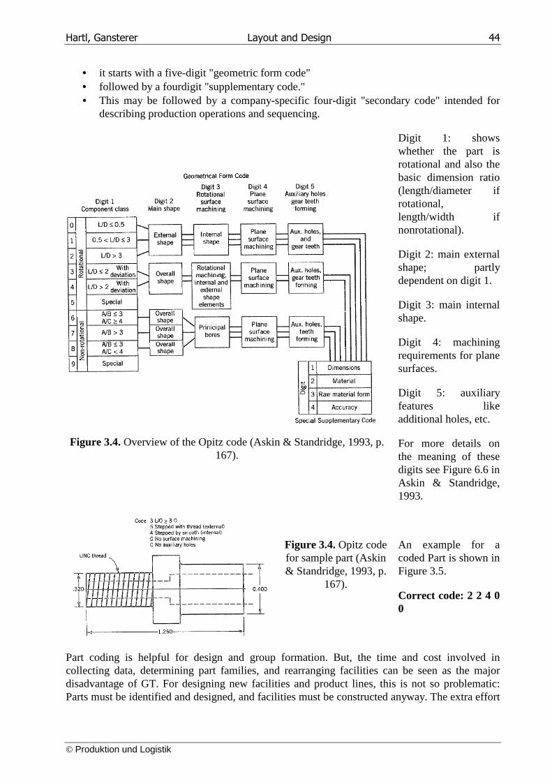
Figure 3.4. Opitz code for sample part (Askin & Standridge, 1993, p.
167).
An example for a coded Part is shown in Figure 3.5.
Correct code: 2 2 4 0 0
Part coding is helpful for design and group formation. But, the time and cost involved in collecting data, determining part families, and rearranging facilities can be seen as the major disadvantage of GT. For designing new facilities and product lines, this is not so problematic: Parts must be identified and designed, and facilities must be constructed anyway. The extra effort
Hartl, Gansterer Layout and Design 45
© Produktion und Logistik
to plan under a GT framework is marginal, and the framework facilitates standardization and operation thereafter. Hence, GT is a logical approach to product and facility planning.
3.4 Classification (group formation)
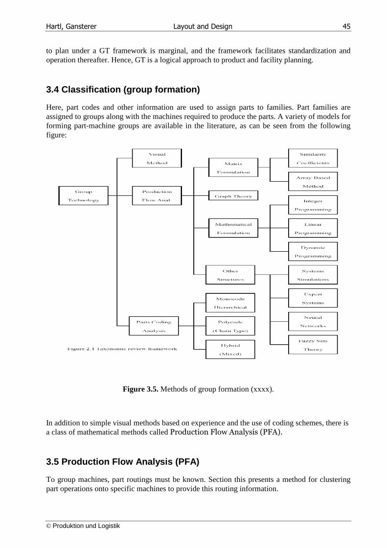
Here, part codes and other information are used to assign parts to families. Part families are assigned to groups along with the machines required to produce the parts. A variety of models for forming part-machine groups are available in the literature, as can be seen from the following figure:
Figure 3.5. Methods of group formation (xxxx).
In addition to simple visual methods based on experience and the use of coding schemes, there is a class of mathematical methods called Production Flow Analysis (PFA).
3.5 Production Flow Analysis (PFA)
To group machines, part routings must be known. Section this presents a method for clustering part operations onto specific machines to provide this routing information.
Hartl, Gansterer Layout and Design 46
© Produktion und Logistik
The basic idea is:
• identify items that are made with the same processes / the same equipment
• These parts are assembled into a part family
• Can be grouped into a cell to minimize material handling requirements.
The clustering methods can be classified into:
• Part family grouping: Form part families and then group machines into cells • Machine grouping: Form machine cells based upon similarities in part routing and then
allocate parts to cells • Machine-part grouping: Form part families and machine cells simultaneously.
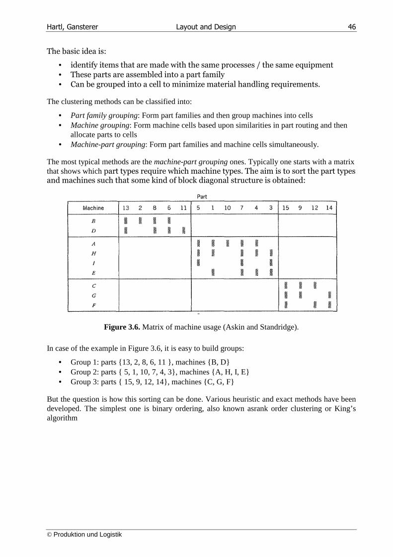
The most typical methods are the machine-part grouping ones. Typically one starts with a matrix that shows which part types require which machine types. The aim is to sort the part types and machines such that some kind of block diagonal structure is obtained:
Figure 3.6. Matrix of machine usage (Askin and Standridge).
In case of the example in Figure 3.6, it is easy to build groups:
• Group 1: parts {13, 2, 8, 6, 11 }, machines {B, D} • Group 2: parts { 5, 1, 10, 7, 4, 3}, machines {A, H, I, E} • Group 3: parts { 15, 9, 12, 14}, machines {C, G, F}
But the question is how this sorting can be done. Various heuristic and exact methods have been developed. The simplest one is binary ordering, also known asrank order clustering or King’s algorithm
Hartl, Gansterer Layout and Design 47
© Produktion und Logistik
3.5.1 Binary Ordering (Rank Order Clustering, King’ s Algorithm)
This is is done in three steps
• Interpret rows and columns as binary numbers • Sort rows w.r.t. decreasing binary numbers • Sort columns w.r.t. decreasing binary numbers
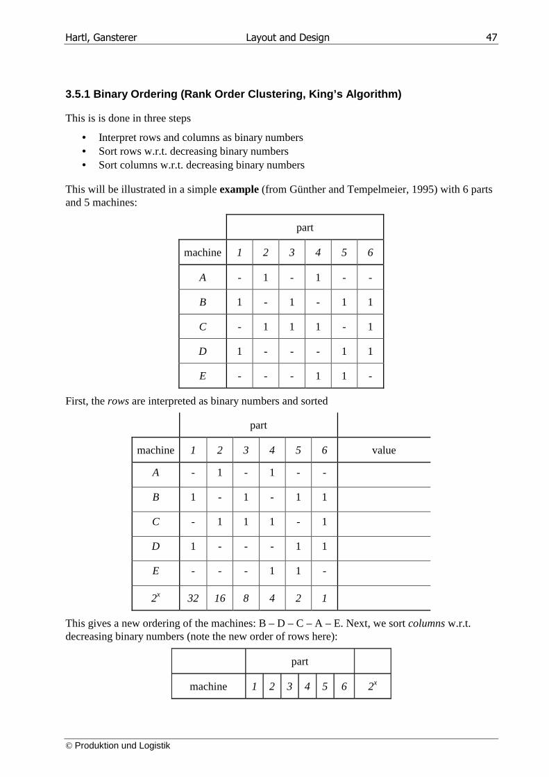
This will be illustrated in a simple example (from Günther and Tempelmeier, 1995) with 6 parts and 5 machines:
part
machine 1 2 3 4 5 6
A - 1 - 1 - -
B 1 - 1 - 1 1
C - 1 1 1 - 1
D 1 - - - 1 1
E - - - 1 1 -
First, the rows are interpreted as binary numbers and sorted
part
machine 1 2 3 4 5 6 value
A - 1 - 1 - -
B 1 - 1 - 1 1
C - 1 1 1 - 1
D 1 - - - 1 1
E - - - 1 1 -
2x 32 16 8 4 2 1
This gives a new ordering of the machines: B – D – C – A – E. Next, we sort columns w.r.t. decreasing binary numbers (note the new order of rows here):
part
machine 1 2 3 4 5 6 2x
Hartl, Gansterer Layout and Design 48
© Produktion und Logistik
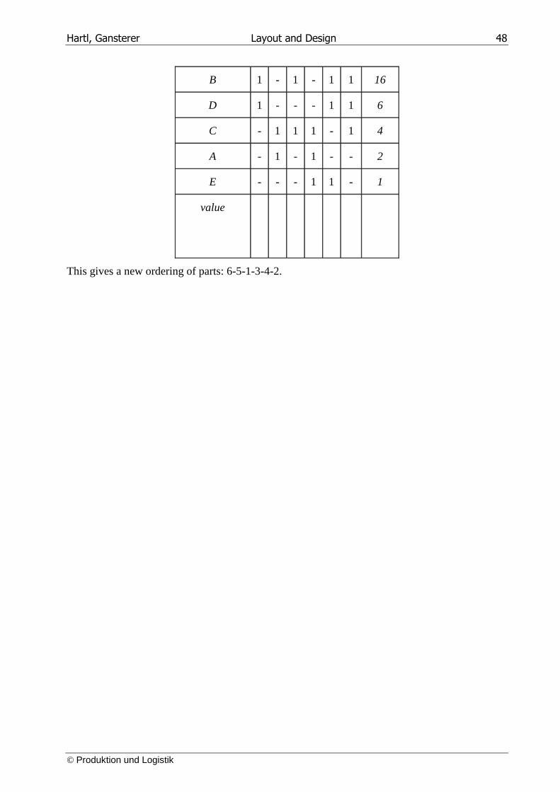
B 1 - 1 - 1 1 16
D 1 - - - 1 1 6
C - 1 1 1 - 1 4
A - 1 - 1 - - 2
E - - - 1 1 - 1
value
This gives a new ordering of parts: 6-5-1-3-4-2.
Hartl, Gansterer Layout and Design 49
© Produktion und Logistik
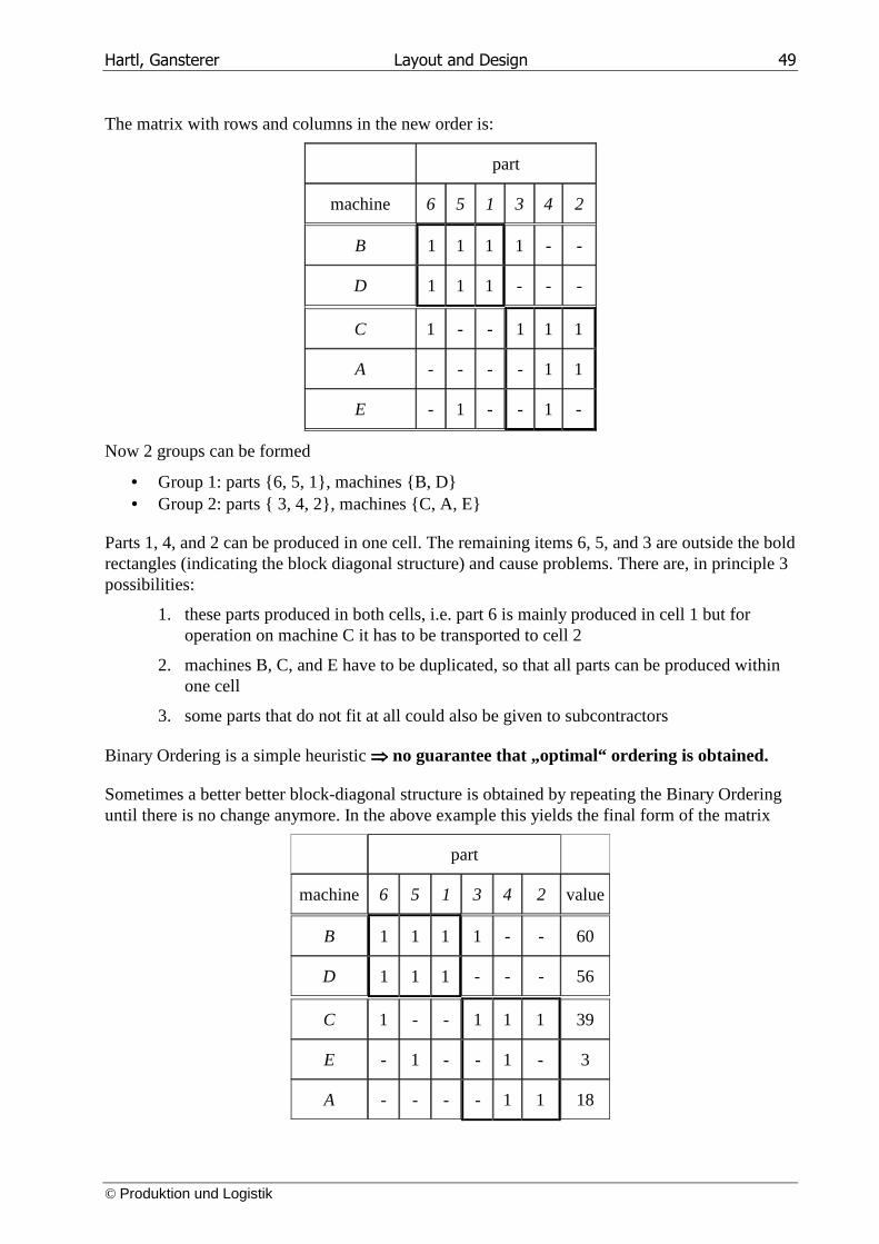
The matrix with rows and columns in the new order is:
part
machine 6 5 1 3 4 2
B 1 1 1 1 - -
D 1 1 1 - - -
C 1 - - 1 1 1
A - - - - 1 1
E - 1 - - 1 -
Now 2 groups can be formed
• Group 1: parts {6, 5, 1}, machines {B, D} • Group 2: parts { 3, 4, 2}, machines {C, A, E}
Parts 1, 4, and 2 can be produced in one cell. The remaining items 6, 5, and 3 are outside the bold rectangles (indicating the block diagonal structure) and cause problems. There are, in principle 3 possibilities:
1. these parts produced in both cells, i.e. part 6 is mainly produced in cell 1 but for operation on machine C it has to be transported to cell 2
2. machines B, C, and E have to be duplicated, so that all parts can be produced within one cell
3. some parts that do not fit at all could also be given to subcontractors
Binary Ordering is a simple heuristic ⇒⇒⇒⇒ no guarantee that „optimal“ ordering is obtained.
Sometimes a better better block-diagonal structure is obtained by repeating the Binary Ordering until there is no change anymore. In the above example this yields the final form of the matrix
part
machine 6 5 1 3 4 2 value
B 1 1 1 1 - - 60
D 1 1 1 - - - 56
C 1 - - 1 1 1 39
E - 1 - - 1 - 3
A - - - - 1 1 18
Hartl, Gansterer Layout and Design 50
© Produktion und Logistik
value 28 26 24 20 7 5
Hence, repeated Binary Ordering did not help in this example.
3.5.2 Single-Pass Heuristic Considering Capacities (Askin and Standridge)
In the previous section we assumed that all machines have sufficient capacity to produce all products that need to go on this machine, i.e. we ignored capacity. The following algorithm by Askin and Standridge extends the model by introducing capacity considerations:
We make the following assumptions:
• All parts must be processed in one cell (machines must be duplicated, if off-diagonal elements occur in the matrix)
• All machines have capacities (normalized to be 1)
• There are constraints on number of identical machines in a group
• There are constraints on total number of machines in a group
Example: We will demonstrate the methods in an example (from Günther and Tempelmeier, 1995) with 7 parts and 6 machines. At most 4 machines can be in a group and not mot than one copy of each machine is allowed in each group. The following matrix contains the processing times (incl. set up times) for typical lot size of parts on machines (i.e., the entries in matrix are not just 0/1 for used/not used). All times are normalized as percentage of total machine capacity:
part
machine 1 2 3 4 5 6 7 sum min. # machines
A 0.3 - - - 0.6 - - 0.9 1
B - 0.3 - 0.3 - - 0.1
C 0.4 - - 0.5 - 0.3 -
D 0.2 - 0.4 - 0.3 - 0.5
E - 0.4 - - - 0.5 -
F - 0.2 0.3 0.4 - - 0.2
By summing up all entries in a row we obtain total machine utilization. If this value exceeds one, at least two machines are needed. More generally, this number must be rounded up to the next integer to give the minimum number of machines needed. It should be noted, that this minimum number of machines is a lower bound. It may be necessary to use more copies of some machines than this minimum number suggests.
Summing up the minimum number of machines for all machine types we obtain, that at least 9 machines are needed. Since not more than 4 machines are permitted in a group, we know that at
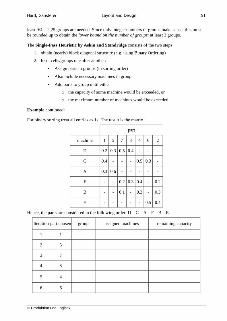
Hartl, Gansterer Layout and Design 51
© Produktion und Logistik
least 9/4 = 2,25 groups are needed. Since only integer numbers of groups make sense, this must be rounded up to obtain the lower bound on the number of groups: at least 3 groups.
The Single-Pass Heuristic by Askin and Standridge consists of the two steps
1. obtain (nearly) block diagonal structure (e.g. using Binary Ordering)
2. form cells/groups one after another:
• Assign parts to groups (in sorting order)
• Also include necessary machines in group
• Add parts to group until either
o the capacity of some machine would be exceeded, or
o the maximum number of machines would be exceeded
Example continued:
For binary sorting treat all entries as 1s. The result is the matrix
part
machine 1 5 7 3 4 6 2
D 0.2 0.3 0.5 0.4 - - -
C 0.4 - - - 0.5 0.3 -
A 0.3 0.6 - - - - -
F - - 0.2 0.3 0.4 - 0.2
B - - 0.1 - 0.3 - 0.3
E - - - - - 0.5 0.4
Hence, the parts are considered in the following order: D – C – A – F – B – E.
Iteration part chosen group assigned machines remaining capacity
1 1
2 5
3 7
4 3
5 4
6 6
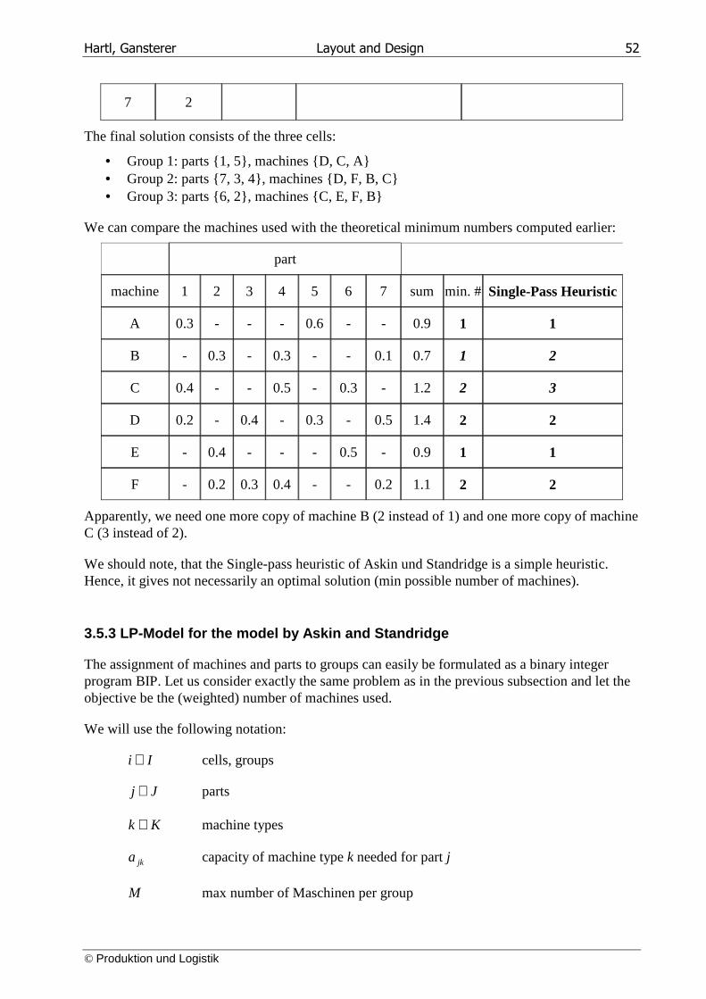
Hartl, Gansterer Layout and Design 52
© Produktion und Logistik
7 2
The final solution consists of the three cells:
• Group 1: parts {1, 5}, machines {D, C, A} • Group 2: parts {7, 3, 4}, machines {D, F, B, C} • Group 3: parts {6, 2}, machines {C, E, F, B}
We can compare the machines used with the theoretical minimum numbers computed earlier:
part
machine 1 2 3 4 5 6 7 sum min. # Single-Pass Heuristic
A 0.3 - - - 0.6 - - 0.9 1 1
B - 0.3 - 0.3 - - 0.1 0.7 1 2
C 0.4 - - 0.5 - 0.3 - 1.2 2 3
D 0.2 - 0.4 - 0.3 - 0.5 1.4 2 2
E - 0.4 - - - 0.5 - 0.9 1 1
F - 0.2 0.3 0.4 - - 0.2 1.1 2 2
Apparently, we need one more copy of machine B (2 instead of 1) and one more copy of machine C (3 instead of 2).
We should note, that the Single-pass heuristic of Askin und Standridge is a simple heuristic. Hence, it gives not necessarily an optimal solution (min possible number of machines).
3.5.3 LP-Model for the model by Askin and Standridg e
The assignment of machines and parts to groups can easily be formulated as a binary integer program BIP. Let us consider exactly the same problem as in the previous subsection and let the objective be the (weighted) number of machines used.
We will use the following notation:
Ii ∈ cells, groups
Jj ∈ parts
Kk ∈ machine types
jka capacity of machine type k needed for part j
M max number of Maschinen per group
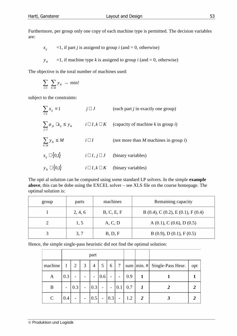
Hartl, Gansterer Layout and Design 53
© Produktion und Logistik
Furthermore, per group only one copy of each machine type is permitted. The decision variables are:
ijx =1, if part j is assigend to group i (and = 0, otherwise)
iky =1, if machine type k is assigend to group i (and = 0, otherwise)
The objective is the toral number of machines used:
→∑∑∈∈ Kk
ikIi
y min!
subject to the constraints:
∑∈
=Ii
ijx 1 Jj ∈ (each part j in exactly one group)
∑∈
≤⋅Jj
ikijjk yxa KkIi ∈∈ , (capacity of machine k in group i)
∑∈
≤Kk
ik My Ii ∈ (not more than M machines in group i)
{ }1,0∈ijx JjIi ∈∈ , (binary variables)
{ }1,0∈iky KkIi ∈∈ , (binary variables)
The opti al solution can be computed using some standard LP solvers. In the simple example above, this can be dobe using the EXCEL solver – see XLS file on the course homepage. The optimal solution is:
group parts machines Remaining capacity
1 2, 4, 6 B, C, E, F B (0.4), C (0.2), E (0.1), F (0.4)
2 1, 5 A, C, D A (0.1), C (0.6), D (0.5)
3 3, 7 B, D, F B (0.9), D (0.1), F (0.5)
Hence, the simple single-pass heuristic did not find the optimal solution:
part
machine 1 2 3 4 5 6 7 sum min. # Single-Pass Heur. opt
A 0.3 - - - 0.6 - - 0.9 1 1 1
B - 0.3 - 0.3 - - 0.1 0.7 1 2 2
C 0.4 - - 0.5 - 0.3 - 1.2 2 3 2
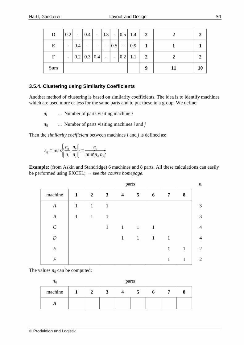
Hartl, Gansterer Layout and Design 54
© Produktion und Logistik
D 0.2 - 0.4 - 0.3 - 0.5 1.4 2 2 2
E - 0.4 - - - 0.5 - 0.9 1 1 1
F - 0.2 0.3 0.4 - - 0.2 1.1 2 2 2
Sum 9 11 10
3.5.4. Clustering using Similarity Coefficients
Another method of clustering is based on similarity coefficients. The idea is to identify machines which are used more or less for the same parts and to put these in a group. We define:
ni ... Number of parts visiting machine i
nij ... Number of parts visiting machines i and j
Then the similarity coefficient between machines i and j is defined as:
{ }ji
ij
j
ij
i
ijij nn
n
n
n
n
ns
,min,max =
=
Example: (from Askin and Standridge) 6 machines and 8 parts. All these calculations can easily be performed using EXCEL; → see the course homepage.
parts ni
machine 1 2 3 4 5 6 7 8
A 1 1 1 3
B 1 1 1 3
C 1 1 1 1 4
D 1 1 1 1 4
E 1 1 2
F 1 1 2
The values nij can be computed:
nij parts
machine 1 2 3 4 5 6 7 8
A
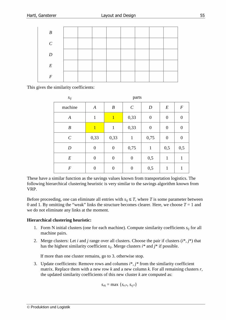
Hartl, Gansterer Layout and Design 55
© Produktion und Logistik
B
C
D
E
F
This gives the similarity coefficients:
sij parts
machine A B C D E F
A 1 1 0,33 0 0 0
B 1 1 0,33 0 0 0
C 0,33 0,33 1 0,75 0 0
D 0 0 0,75 1 0,5 0,5
E 0 0 0 0,5 1 1
F 0 0 0 0,5 1 1
These have a similar function as the savings values known from transportation logistics. The following hierarchical clustering heuristic is very similar to the savings algorithm known from VRP.
Before proceeding, one can eliminate all entries with sij ≤ T, where T is some parameter between 0 and 1. By omitting the “weak” links the structure becomes clearer. Here, we choose T = 1 and we do not eliminate any links at the moment.
Hierarchical clustering heuristic:
1. Form N initial clusters (one for each machine). Compute similarity coefficients sij for all machine pairs.
2. Merge clusters: Let i and j range over all clusters. Choose the pair if clusters (i*, j*) that has the highest similarity coefficient sij. Merge clusters i* and j* if possible.
If more than one cluster remains, go to 3. otherwise stop.
3. Update coefficients: Remove rows and columns i*, j* from the similarity coefficient matrix. Replace them with a new row k and a new column k. For all remaining clusters r, the updated similarity coefficients of this new cluster k are computed as:
srk = max {sri* , srj* }
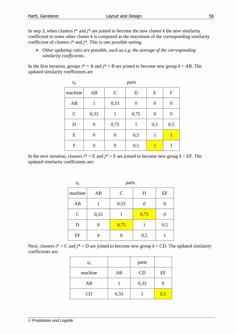
Hartl, Gansterer Layout and Design 56
© Produktion und Logistik
In step 3, when clusters i* and j* are joined to become the new cluster k the new similarity coefficient to some other cluster k is computed as the maximum of the corresponding similarity coefficient of clusters i* and j*. This is one possible setting.
� Other updating rules are possible, such as e.g. the average of the corresponding similarity coefficients.
In the first iteration, groups i* = A and j* = B are joined to become new group k = AB. The updated similarity coefficients are
sij parts
machine AB C D E F
AB 1 0,33 0 0 0
C 0,33 1 0,75 0 0
D 0 0,75 1 0,5 0,5
E 0 0 0,5 1 1
F 0 0 0,5 1 1
In the next iteration, clusters i* = E and j* = F are joined to become new group k = EF. The updated similarity coefficients are:
sij parts
machine AB C D EF
AB 1 0,33 0 0
C 0,33 1 0,75 0
D 0 0,75 1 0,5
EF 0 0 0,5 1
Next, clusters i* = C and j* = D are joined to become new group k = CD. The updated similarity coefficients are:
sij parts
machine AB CD EF
AB 1 0,33 0
CD 0,33 1 0,5
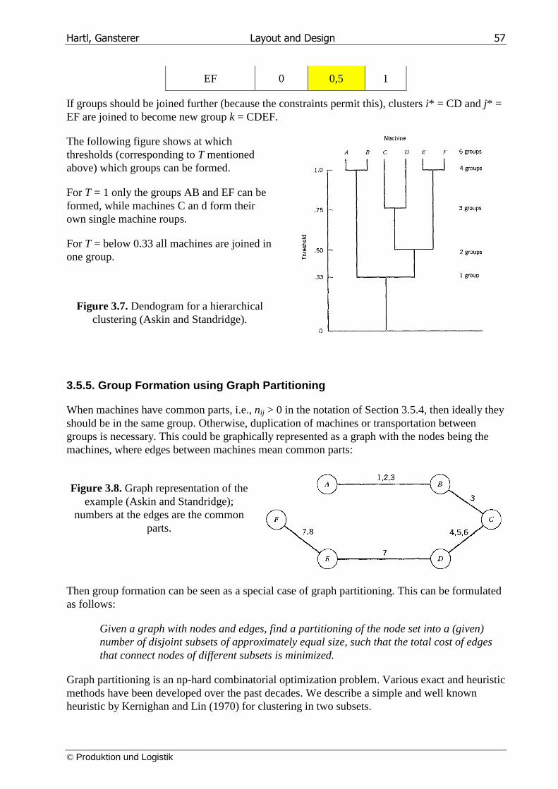
Hartl, Gansterer Layout and Design 57
© Produktion und Logistik
EF 0 0,5 1
If groups should be joined further (because the constraints permit this), clusters i* = CD and j* = EF are joined to become new group k = CDEF.
The following figure shows at which thresholds (corresponding to T mentioned above) which groups can be formed.
For T = 1 only the groups AB and EF can be formed, while machines C an d form their own single machine roups.
For T = below 0.33 all machines are joined in one group.
Figure 3.7. Dendogram for a hierarchical clustering (Askin and Standridge).
3.5.5. Group Formation using Graph Partitioning
When machines have common parts, i.e., nij > 0 in the notation of Section 3.5.4, then ideally they should be in the same group. Otherwise, duplication of machines or transportation between groups is necessary. This could be graphically represented as a graph with the nodes being the machines, where edges between machines mean common parts:
Figure 3.8. Graph representation of the example (Askin and Standridge);
numbers at the edges are the common parts.
Then group formation can be seen as a special case of graph partitioning. This can be formulated as follows:
Given a graph with nodes and edges, find a partitioning of the node set into a (given) number of disjoint subsets of approximately equal size, such that the total cost of edges that connect nodes of different subsets is minimized.
Graph partitioning is an np-hard combinatorial optimization problem. Various exact and heuristic methods have been developed over the past decades. We describe a simple and well known heuristic by Kernighan and Lin (1970) for clustering in two subsets.
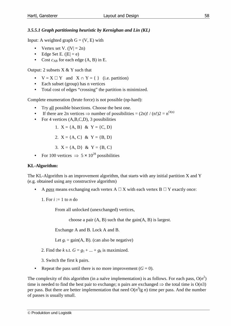
Hartl, Gansterer Layout and Design 58
© Produktion und Logistik
3.5.5.1 Graph partitioning heuristic by Kernighan and Lin (KL)
Input: A weighted graph G = (V, E) with
• Vertex set V. (|V| = 2n) • Edge Set E. (|E| = e) • Cost cAB for each edge (A, B) in E.
Output: 2 subsets X & Y such that
• V = X ∪ Y and X ∩ Y = { } (i.e. partition) • Each subset (group) has n vertices • Total cost of edges “crossing” the partition is minimized.
Complete enumeration (brute force) is not possible (np-hard):
• Try all possible bisections. Choose the best one. • If there are 2n vertices ⇒ number of possibilities = (2n)! / (n!)2 = nO(n) • For 4 vertices (A,B,C,D), 3 possibilities
1. X = {A, B} & Y = {C, D}
2. X = {A, C} & Y = {B, D}
3. X = {A, D} & Y = {B, C}
• For 100 vertices ⇒ 5 × 1028 possibilities
KL-Algorithm:
The KL-Algorithm is an improvement algorithm, that starts with any initial partition X and Y (e.g. obtained using any constructive algorithm)
• A pass means exchanging each vertex A ∈ X with each vertex B ∈ Y exactly once:
1. For i := 1 to n do
From all unlocked (unexchanged) vertices,
choose a pair (A, B) such that the gain(A, B) is largest.
Exchange A and B. Lock A and B.
Let gi = gain(A, B). (can also be negative)
2. Find the k s.t. G = g1 + ... + gk is maximized.
3. Switch the first k pairs.
• Repeat the pass until there is no more improvement (G = 0).
The complexity of this algorithm (in a naïve implementation) is as follows. For each pass, O(n2) time is needed to find the best pair to exchange; n pairs are exchanged ⇒ the total time is O(n3) per pass. But there are better implementation that need O(n2lg n) time per pass. And the number of passes is usually small.
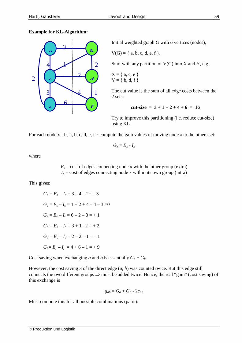
Hartl, Gansterer Layout and Design 59
© Produktion und Logistik
Example for KL-Algorithm:
Initial weighted graph G with 6 vertices (nodes),
V(G) = { a, b, c, d, e, f }.
Start with any partition of V(G) into X and Y, e.g.,
X = { a, c, e } Y = { b, d, f }
The cut value is the sum of all edge costs between the 2 sets:
cut-size = 3 + 1 + 2 + 4 + 6 = 16
Try to improve this partitioning (i.e. reduce cut-size) using KL.
For each node x ∈ { a, b, c, d, e, f }.compute the gain values of moving node x to the others set:
Gx = Ex - Ix
where
Ex = cost of edges connecting node x with the other group (extra) Ix = cost of edges connecting node x within its own group (intra)
This gives:
Ga = Ea – Ia = 3 – 4 – 2= – 3
Gc = Ec – Ic = 1 + 2 + 4 – 4 – 3 =0
Ge = Ee – Ie = 6 – 2 – 3 = + 1
Gb = Eb – Ib = 3 + 1 –2 = + 2
Gd = Ed – Id = 2 – 2 – 1 = – 1
Gf = Ef – If = 4 + 6 – 1 = + 9
Cost saving when exchanging a and b is essentially Ga + Gb
However, the cost saving 3 of the direct edge (a, b) was counted twice. But this edge still connects the two different groups ⇒ must be added twice. Hence, the real “gain” (cost saving) of this exchange is
gab = Ga + Gb - 2cab
Must compute this for all possible combinations (pairs):
a
c
b
d
e f
3
1
2
4
3 4
6
2
1
2
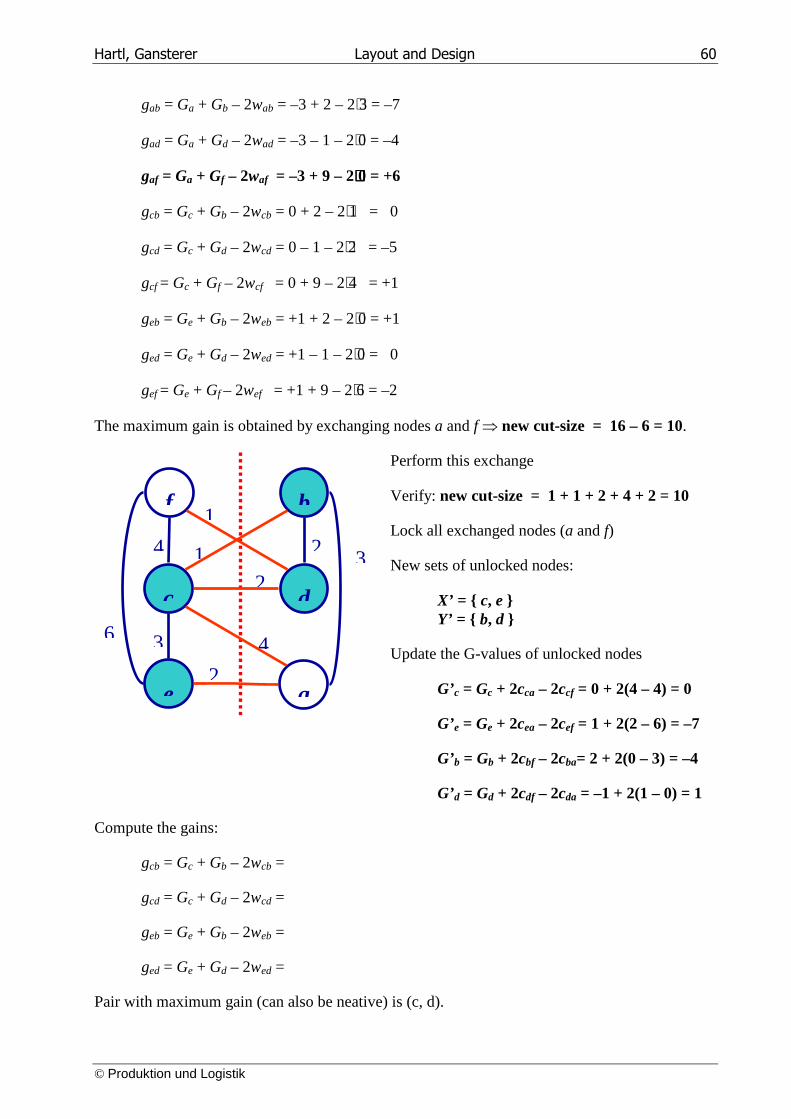
Hartl, Gansterer Layout and Design 60
© Produktion und Logistik
gab = Ga + Gb – 2wab = –3 + 2 – 2⋅3 = –7
gad = Ga + Gd – 2wad = –3 – 1 – 2⋅0 = –4
gaf = Ga + Gf – 2waf = –3 + 9 – 2⋅⋅⋅⋅0 = +6
gcb = Gc + Gb – 2wcb = 0 + 2 – 2⋅1 = 0
gcd = Gc + Gd – 2wcd = 0 – 1 – 2⋅2 = –5
gcf = Gc + Gf – 2wcf = 0 + 9 – 2⋅4 = +1
geb = Ge + Gb – 2web = +1 + 2 – 2⋅0 = +1
ged = Ge + Gd – 2wed = +1 – 1 – 2⋅0 = 0
gef = Ge + Gf – 2wef = +1 + 9 – 2⋅6 = –2
The maximum gain is obtained by exchanging nodes a and f ⇒ new cut-size = 16 – 6 = 10.
Perform this exchange
Verify: new cut-size = 1 + 1 + 2 + 4 + 2 = 10
Lock all exchanged nodes (a and f)
New sets of unlocked nodes:
X’ = { c, e } Y’ = { b, d }
Update the G-values of unlocked nodes
G’c = Gc + 2cca – 2ccf = 0 + 2(4 – 4) = 0
G’e = Ge + 2cea – 2cef = 1 + 2(2 – 6) = –7
G’b = Gb + 2cbf – 2cba= 2 + 2(0 – 3) = –4
G’d = Gd + 2cdf – 2cda = –1 + 2(1 – 0) = 1
Compute the gains:
gcb = Gc + Gb – 2wcb =
gcd = Gc + Gd – 2wcd =
geb = Ge + Gb – 2web =
ged = Ge + Gd – 2wed =
Pair with maximum gain (can also be neative) is (c, d).
a
c
b
d
e
f
3
1
2
4
3 4 6
2 1
2
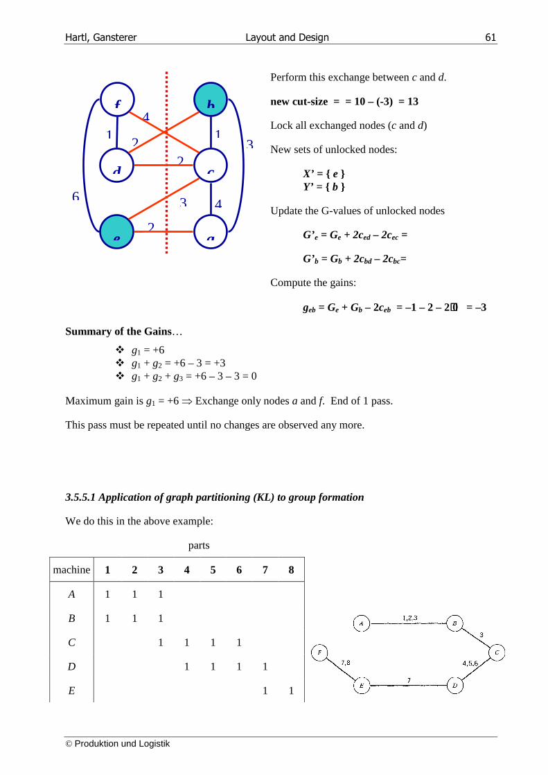
Hartl, Gansterer Layout and Design 61
© Produktion und Logistik
Perform this exchange between c and d.
new cut-size = = 10 – (-3) = 13
Lock all exchanged nodes (c and d)
New sets of unlocked nodes:
X’ = { e } Y’ = { b }
Update the G-values of unlocked nodes
G’e = Ge + 2ced – 2cec =
G’b = Gb + 2cbd – 2cbc=
Compute the gains:
geb = Ge + Gb – 2ceb = –1 – 2 – 2⋅⋅⋅⋅0 = –3
Summary of the Gains…
� g1 = +6 � g1 + g2 = +6 – 3 = +3 � g1 + g2 + g3 = +6 – 3 – 3 = 0
Maximum gain is g1 = +6 ⇒ Exchange only nodes a and f. End of 1 pass.
This pass must be repeated until no changes are observed any more.
3.5.5.1 Application of graph partitioning (KL) to group formation
We do this in the above example:
parts
machine 1 2 3 4 5 6 7 8
A 1 1 1
B 1 1 1
C 1 1 1 1
D 1 1 1 1
E 1 1
a
d
b
c
e
f
3 1
2
4
3 4 6
2 1
2
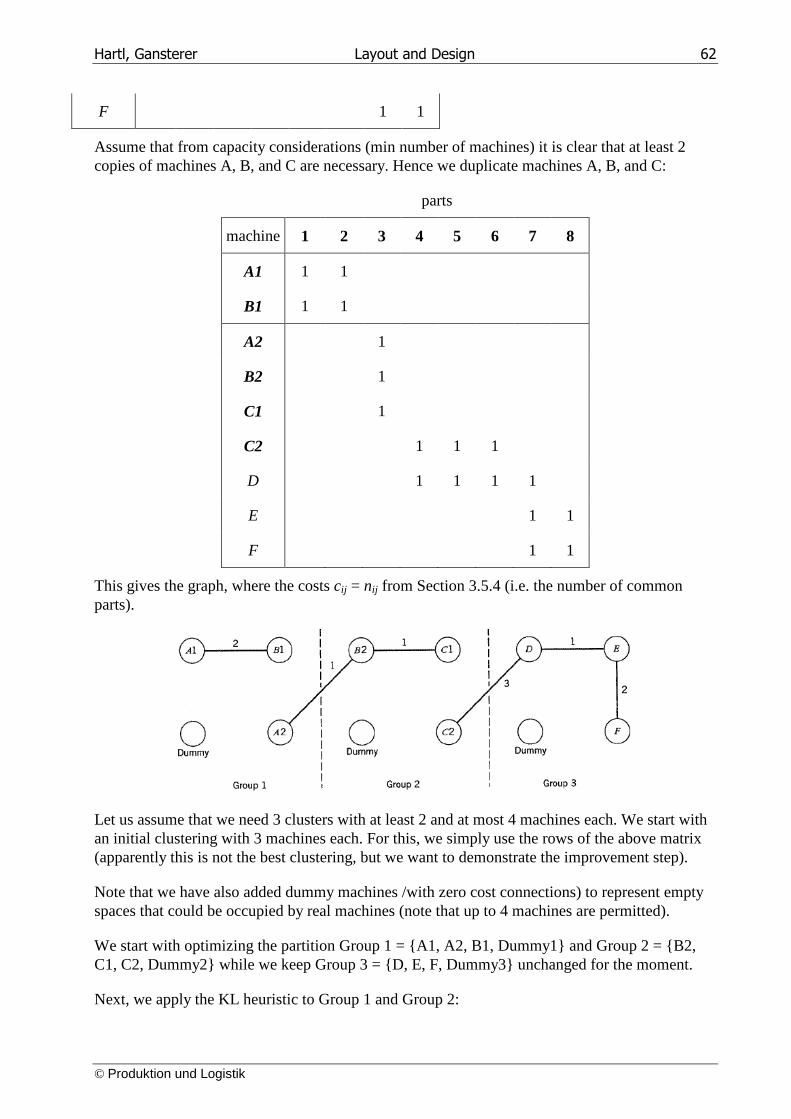
Hartl, Gansterer Layout and Design 62
© Produktion und Logistik
F 1 1
Assume that from capacity considerations (min number of machines) it is clear that at least 2 copies of machines A, B, and C are necessary. Hence we duplicate machines A, B, and C:
parts
machine 1 2 3 4 5 6 7 8
A1 1 1
B1 1 1
A2 1
B2 1
C1 1
C2 1 1 1
D 1 1 1 1
E 1 1
F 1 1
This gives the graph, where the costs cij = nij from Section 3.5.4 (i.e. the number of common parts).
Let us assume that we need 3 clusters with at least 2 and at most 4 machines each. We start with an initial clustering with 3 machines each. For this, we simply use the rows of the above matrix (apparently this is not the best clustering, but we want to demonstrate the improvement step).
Note that we have also added dummy machines /with zero cost connections) to represent empty spaces that could be occupied by real machines (note that up to 4 machines are permitted).
We start with optimizing the partition Group 1 = {A1, A2, B1, Dummy1} and Group 2 = {B2, C1, C2, Dummy2} while we keep Group 3 = {D, E, F, Dummy3} unchanged for the moment.
Next, we apply the KL heuristic to Group 1 and Group 2:
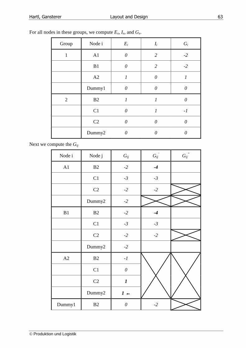
Hartl, Gansterer Layout and Design 63
© Produktion und Logistik
For all nodes in these groups, we compute Ex, Ix, and Gx.
Group Node i Ei I i Gi
1 A1 0 2 -2
B1 0 2 -2
A2 1 0 1
Dummy1 0 0 0
2 B2 1 1 0
C1 0 1 -1
C2 0 0 0
Dummy2 0 0 0
Next we compute the Gij
Node i Node j Gij Gij’ Gij
”
A1 B2 -2 -4
C1 -3 -3
C2 -2 -2
Dummy2 -2
B1 B2 -2 -4
C1 -3 -3
C2 -2 -2
Dummy2 -2
A2 B2 -1
C1 0
C2 1
Dummy2 1 ←←←←
Dummy1 B2 0 -2
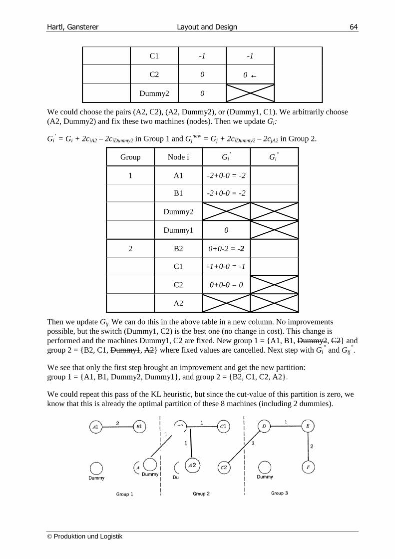
Hartl, Gansterer Layout and Design 64
© Produktion und Logistik
C1 -1 -1
C2 0 0 ←←←←
Dummy2 0
We could choose the pairs (A2, C2), (A2, Dummy2), or (Dummy1, C1). We arbitrarily choose (A2, Dummy2) and fix these two machines (nodes). Then we update Gi:
Gi’ = Gi + 2ciA2 – 2ciDummy2 in Group 1 and Gj
new = Gj + 2ciDummy2 – 2cjA2 in Group 2.
Group Node i Gi’ Gi
”
1 A1 -2+0-0 = -2
B1 -2+0-0 = -2
Dummy2
Dummy1 0
2 B2 0+0-2 = -2
C1 -1+0-0 = -1
C2 0+0-0 = 0
A2
Then we update Gij. We can do this in the above table in a new column. No improvements possible, but the switch (Dummy1, C2) is the best one (no change in cost). This change is performed and the machines Dummy1, C2 are fixed. New group 1 = {A1, B1, Dummy2, C2} and group 2 = {B2, C1, Dummy1, A2} where fixed values are cancelled. Next step with Gi
” and Gij” .
We see that only the first step brought an improvement and get the new partition: group 1 = {A1, B1, Dummy2, Dummy1}, and group 2 = {B2, C1, C2, A2}.
We could repeat this pass of the KL heuristic, but since the cut-value of this partition is zero, we know that this is already the optimal partition of these 8 machines (including 2 dummies).
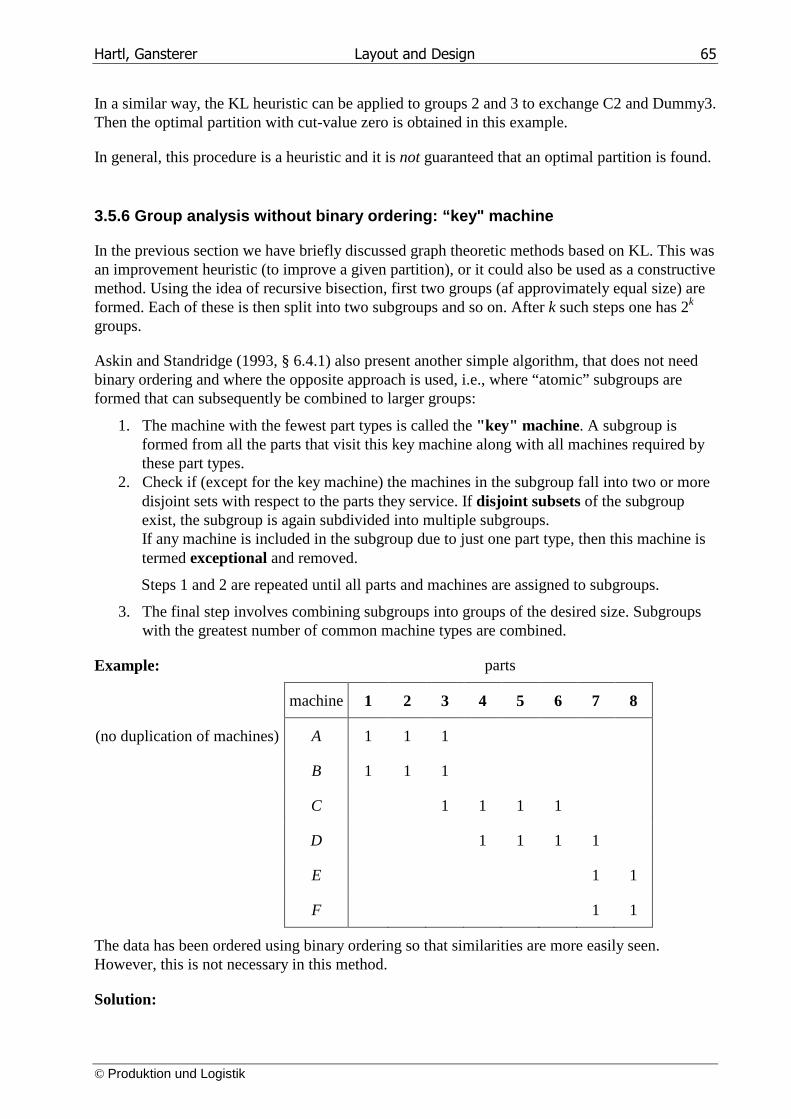
Hartl, Gansterer Layout and Design 65
© Produktion und Logistik
In a similar way, the KL heuristic can be applied to groups 2 and 3 to exchange C2 and Dummy3. Then the optimal partition with cut-value zero is obtained in this example.
In general, this procedure is a heuristic and it is not guaranteed that an optimal partition is found.
3.5.6 Group analysis without binary ordering: “key" machine
In the previous section we have briefly discussed graph theoretic methods based on KL. This was an improvement heuristic (to improve a given partition), or it could also be used as a constructive method. Using the idea of recursive bisection, first two groups (af approvimately equal size) are formed. Each of these is then split into two subgroups and so on. After k such steps one has 2k
groups.
Askin and Standridge (1993, § 6.4.1) also present another simple algorithm, that does not need binary ordering and where the opposite approach is used, i.e., where “atomic” subgroups are formed that can subsequently be combined to larger groups:
1. The machine with the fewest part types is called the "key" machine . A subgroup is formed from all the parts that visit this key machine along with all machines required by these part types.
2. Check if (except for the key machine) the machines in the subgroup fall into two or more disjoint sets with respect to the parts they service. If disjoint subsets of the subgroup exist, the subgroup is again subdivided into multiple subgroups. If any machine is included in the subgroup due to just one part type, then this machine is termed exceptional and removed.
Steps 1 and 2 are repeated until all parts and machines are assigned to subgroups.
3. The final step involves combining subgroups into groups of the desired size. Subgroups with the greatest number of common machine types are combined.
Example: parts
machine 1 2 3 4 5 6 7 8
(no duplication of machines) A 1 1 1
B 1 1 1
C 1 1 1 1
D 1 1 1 1
E 1 1
F 1 1
The data has been ordered using binary ordering so that similarities are more easily seen. However, this is not necessary in this method.
Solution:
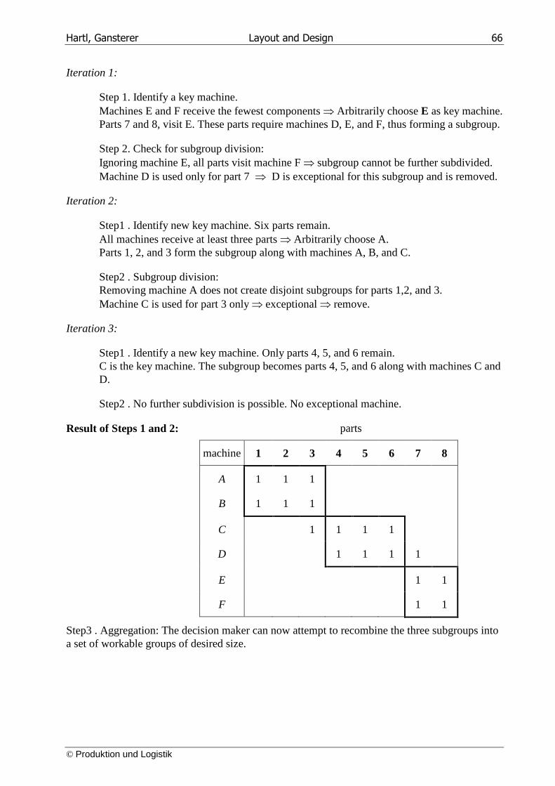
Hartl, Gansterer Layout and Design 66
© Produktion und Logistik
Iteration 1:
Step 1. Identify a key machine. Machines E and F receive the fewest components ⇒ Arbitrarily choose E as key machine. Parts 7 and 8, visit E. These parts require machines D, E, and F, thus forming a subgroup.
Step 2. Check for subgroup division: Ignoring machine E, all parts visit machine F ⇒ subgroup cannot be further subdivided. Machine D is used only for part 7 ⇒ D is exceptional for this subgroup and is removed.
Iteration 2:
Step1 . Identify new key machine. Six parts remain. All machines receive at least three parts ⇒ Arbitrarily choose A. Parts 1, 2, and 3 form the subgroup along with machines A, B, and C.
Step2 . Subgroup division: Removing machine A does not create disjoint subgroups for parts 1,2, and 3. Machine C is used for part 3 only ⇒ exceptional ⇒ remove.
Iteration 3:
Step1 . Identify a new key machine. Only parts 4, 5, and 6 remain. C is the key machine. The subgroup becomes parts 4, 5, and 6 along with machines C and D.
Step2 . No further subdivision is possible. No exceptional machine.
Result of Steps 1 and 2: parts
machine 1 2 3 4 5 6 7 8
A 1 1 1
B 1 1 1
C 1 1 1 1
D 1 1 1 1
E 1 1
F 1 1
Step3 . Aggregation: The decision maker can now attempt to recombine the three subgroups into a set of workable groups of desired size.
Hartl, Gansterer Layout and Design 67
© Produktion und Logistik
3.6 Metaheuristics
We have briefly discussed some of the classical constructive heuristics and improvement heuristics from the literature.
Since we are dealing with a tactical problem (that is not solved every day) where long computation times are acceptable, it makes sense to invest more time. This can be done by applying metaheuristics, exact methods (up to a certain problem size) and combined methods (matheuristics).
There is a large literature on applying metaheuristics and grouping or clustering problems (mainly genetic algorithms or tabu search). Nevertheless, various possibilities exist to come up with new metaheuristic approaches.
Examples:
• Since the similarity coefficients are rather similar to the savings values of transportation logistics (VRP), the idea of a savings based ant system for VRP could be transferred to grouping problems.
• The KL algorithm could be considered a local search (maybe in a simplified faster version), and could be combined with some larger shaking steps to a VNS. Other fast local searches (exchange and move) could be considered.
• A matheuristic could easily be constructed by applying e.g. the principle of destroy and reconstruct: for a large problem, a subset of groups could be “destroyed” and all their machines and parts could be freed. Then this smaller problem (considering only these parts and machines) could be solved using some exact algorithm (e.g. applying CPLEX to a MIP formulation).
When designing metaheuristics or matheuristics for grouping problems, there are also 2 possibilities:
• Work directly on the model formulation (e.g. the above examples)
• Use a more aggregated representation and then apply some constructive algorithm to compute the solution out of it. For example, the metaheuristic could just work on the ordering of parts and machines (to give a better block diagonal structure than binary ordering) and then the single pass heuristic by Askin and Standridge could be used to construct a solution.
It should also be noted that there ate various classes of grouping problems that differ w.r.t. objective and constraints. This concerns e.g. duplication of machines and/or inter-group transport, etc.
References
Askin, R.G., Standridge, C.R.: Modeling & Analysis Of Manufacturing Systems, John Wiley & Sons, 1993.
Hartl, Gansterer Layout and Design 68
© Produktion und Logistik
B. Kernighan and S. Lin (1970): An Efficient Heuristic Procedure for Partitioning of Electrical Circuits, Bell System Technical Journal, 291-307.
Internet sources on Opiz, KK3 und some methods, e.g.:
• http://www.ielm.ust.hk/dfaculty/ajay/courses/ieem513/GT/GT.html
Examples for metaheuristics:
• T.L. James, E.C. Brown, K.B. Keeling (2007): A hybrid grouping genetic algorithm for the cell formation problem, Computers and Operations Research, Volume 34 (7, July) 2059-2079 .
• Mahdavi, M.M. Paydar, M. Solimanpur, A. Heidarzade (2009): Genetic algorithm approach for solving a cell formation problem in cellular manufacturing, Expert Systems with Applications: An International Journal, Volume 36 (3, April) 6598-6604.
• T. Tunnukij, C. Hicks (2009): An Enhanced Grouping Genetic Algorithm for solving the cell formation problem, International Journal of Production Research, Volume 47 (7, Jan.) 1989 – 2007.
• D. Cao and M. Chen (2004): Using penalty function and Tabu search to solve cell formation problems with fixed cell cost, Computers & Operations Research, Volume 31 (1, Jan.) 21-37.
• J. Schaller (2005): Tabu search procedures for the cell formation problem with intra-cell transfer costs as a function of cell size, Computers and Industrial Engineering, Volume 49 (3, Nov.), 449 – 462.
Hartl, Gansterer Layout and Design 69
© Produktion und Logistik
4. Exact Methods for Assembly Line Balancing We have seen in the beginning of this chapter, that an Assembly Line Balancing (ALB) problem can be represented as a binary LP. Smaller instances can be simply solved by using a general purpose LP-solver. For very large instances of this np-hard problem, heuristics need to be used - see the previous sections.
Since ALB problems are tactical problems that are solved only now and then, the results need not be available very soon and computation time can in principle be quite long.
Hence, a number of tailored exact methods have been developed for ALB problems. The most well known ones are based on Dynamic Programming (DP) and Branch & Bound (B&B). In the next subsections we present two such algorithms for Alternative 1, i.e. where the cycle time is given and the number of stations has to be minimized.
Jackson Algorithm (Dynamic Programming, Decision Tree)
This was the first and simplest exact method that was specially designed for ALB problems. Later improved algorithms have been suggested but the dominance rules are still of general relevance.
Construction of a Decision Tree
The individual stations of the assembly-line are considered one by one.
In the first stage one generates all possibilities for the allocation of the first station, where one considers only maximal stations (i.e. no additional operations can be added). Hence, one obtains a number of different states, which are described by the operations already assigned to station 1.
Step from stage k-1 to stage k:
The state in stage k-1 represents all operations already assigned to stations 1 to k-1 (not only k).
In stage k, for each such state in stage k-1, one forms all maximal stations k and obtains the corresponding states in stage k.
As soon as a state is reached where all operations have been assigned, the optimal solution is reached and k is the minimal number of stations.
As usual in DP, the allocations of the individual stations can be determined by backtracking.
The problem can also be considered as a shortest path problem with nodes being the states and the edges representing the allocations of the stations. The starting node is the empty set and the terminal node represents the situation where all operations are assigned.
Jackson Algorithm
Given:
c … cycle time
A = {1, … , n} … set of all operations with
tj ... durations tj ≤ c;
Precedence graph (i.e. set of all immediate predecessors V(j) or successors N(j))
Notation used:
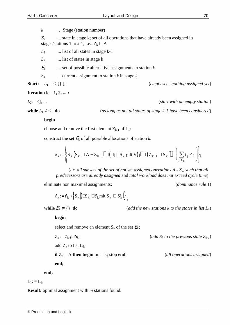
Hartl, Gansterer Layout and Design 70
© Produktion und Logistik
k … Stage (station number)
Zk ... state in stage k; set of all operations that have already been assigned in stages/stations 1 to k-1, i.e.. Zk ⊆ A
L1 ... list of all states in stage k-1
L2 ... list of states in stage k
Ek ... set of possible alternative assignments to station k
Sk ... current assignment to station k in stage k
Start: L1:= < {} ]; (empty set - nothing assigned yet)
Iteration k = 1, 2, ... :
L2:= <]; ... (start with an empty station)
while L1 ≠ < ] do (as long as not all states of stage k-1 have been considered)
begin
choose and remove the first element Zk-1 of L1:
construct the set Ek of all possible allocations of station k:
( ) ( ) ( )( )Ek k k k 1 k k 1 k jj S
: S S A Z j S gilt V j Z S t ck
= ⊆ − ∧ ∀ ∈ ⊆ ∪ ∧ ≤
− −
∈∑ ;
(i.e. all subsets of the set of not yet assigned operations A - Zk, such that all predecessors are already assigned and total workload does not exceed cycle time)
eliminate non maximal assignments: (dominance rule 1)
( ){ }E E Ek k k k k k k: \ S S mit S S= ∃ ′ ∈ ⊂ ′ ;
while Ek ≠ {} do (add the new stations k to the states in list L2)
begin
select and remove an element Sk of the set Ek;
Zk := Zk-1∪Sk; (add Sk to the previous state Zk-1)
add Zk to list L2;
if Zk = A then begin m: = k; stop end; (all operations assigned)
end;
end;
L1: = L2;
Result: optimal assignment with m stations found.
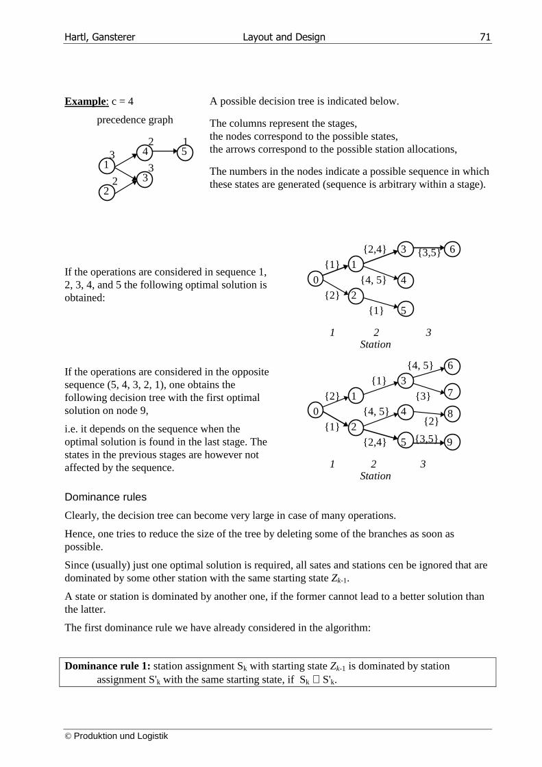
Hartl, Gansterer Layout and Design 71
© Produktion und Logistik
Example: c = 4
precedence graph
2 1 3 4 51 3 2 32
A possible decision tree is indicated below.
The columns represent the stages, the nodes correspond to the possible states, the arrows correspond to the possible station allocations,
The numbers in the nodes indicate a possible sequence in which these states are generated (sequence is arbitrary within a stage).
If the operations are considered in sequence 1, 2, 3, 4, and 5 the following optimal solution is obtained:
{2,4} 3 {3,5} 6
{1} 1
0 {4, 5} 4
{2} 2
{1} 5
1 2 3 Station
If the operations are considered in the opposite sequence (5, 4, 3, 2, 1), one obtains the following decision tree with the first optimal solution on node 9,
i.e. it depends on the sequence when the optimal solution is found in the last stage. The states in the previous stages are however not affected by the sequence.
{4, 5} 6
{1} 3
{2} 1 {3} 7
0 {4, 5} 4 8 {1} 2 {2}
{2,4} 5 {3,5} 9
1 2 3 Station
Dominance rules
Clearly, the decision tree can become very large in case of many operations.
Hence, one tries to reduce the size of the tree by deleting some of the branches as soon as possible.
Since (usually) just one optimal solution is required, all sates and stations cen be ignored that are dominated by some other station with the same starting state Zk-1.
A state or station is dominated by another one, if the former cannot lead to a better solution than the latter.
The first dominance rule we have already considered in the algorithm:
Dominance rule 1: station assignment Sk with starting state Zk-1 is dominated by station assignment S'k with the same starting state, if Sk ⊂ S'k.
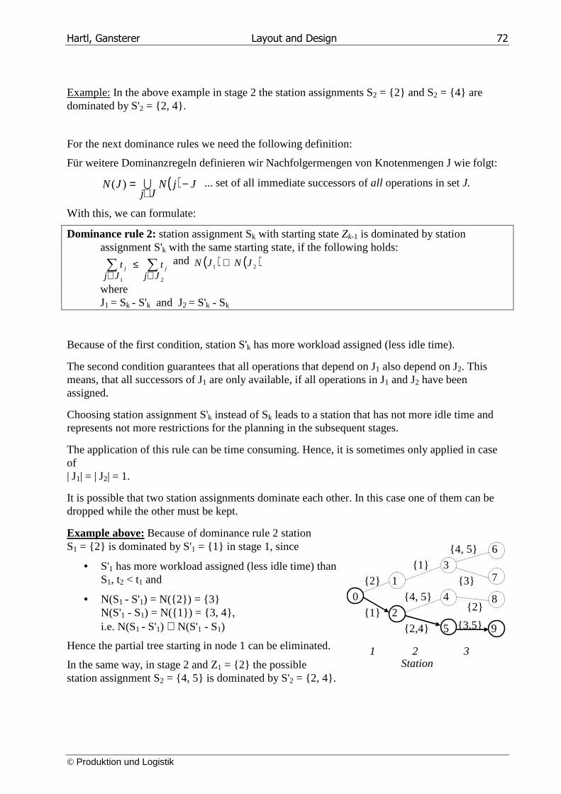
Hartl, Gansterer Layout and Design 72
© Produktion und Logistik
Example: In the above example in stage 2 the station assignments S2 = {2} and S2 = {4} are dominated by S'2 = {2, 4}.
For the next dominance rules we need the following definition:
Für weitere Dominanzregeln definieren wir Nachfolgermengen von Knotenmengen J wie folgt:
( ) JjNJj
JN −∈
= U)( ... set of all immediate successors of all operations in set J.
With this, we can formulate:
Dominance rule 2: station assignment Sk with starting state Zk-1 is dominated by station assignment S'k with the same starting state, if the following holds:
∑∑∈
≤∈ 21 Jj
tJj
t jj and ( ) ( )21 JNJN ⊆
where J1 = Sk - S'k and J2 = S'k - Sk
Because of the first condition, station S'k has more workload assigned (less idle time).
The second condition guarantees that all operations that depend on J1 also depend on J2. This means, that all successors of J1 are only available, if all operations in J1 and J2 have been assigned.
Choosing station assignment S'k instead of Sk leads to a station that has not more idle time and represents not more restrictions for the planning in the subsequent stages.
The application of this rule can be time consuming. Hence, it is sometimes only applied in case of | J1| = | J2| = 1.
It is possible that two station assignments dominate each other. In this case one of them can be dropped while the other must be kept.
Example above: Because of dominance rule 2 station S1 = {2} is dominated by S'1 = {1} in stage 1, since
• S'1 has more workload assigned (less idle time) than S1, t2 < t1 and
• N(S1 - S'1) = N({2}) = {3} N(S'1 - S1) = N({1}) = {3, 4}, i.e. N(S1 - S'1) ⊂ N(S'1 - S1)
Hence the partial tree starting in node 1 can be eliminated.
In the same way, in stage 2 and Z1 = {2} the possible station assignment S2 = {4, 5} is dominated by S'2 = {2, 4}.
{4, 5} 6
{1} 3
{2} 1 {3} 7
0 {4, 5} 4 8
{1} 2 {2}
{2,4} 5 {3,5} 9
1 2 3 Station
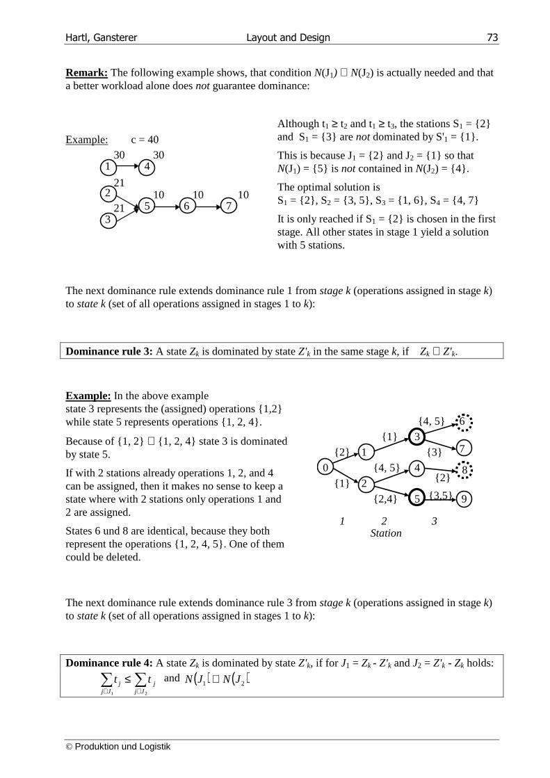
Hartl, Gansterer Layout and Design 73
© Produktion und Logistik
Remark: The following example shows, that condition N(J1) ⊆ N(J2) is actually needed and that a better workload alone does not guarantee dominance:
Example: c = 40 30 301 4 212 10 10 10 21 5 6 73
Although t1 ≥ t2 and t1 ≥ t3, the stations S1 = {2} and S1 = {3} are not dominated by S'1 = {1}.
This is because J1 = {2} and J2 = {1} so that N(J1) = {5} is not contained in N(J2) = {4}.
The optimal solution is S1 = {2}, S2 = {3, 5}, S3 = {1, 6}, S4 = {4, 7}
It is only reached if S1 = {2} is chosen in the first stage. All other states in stage 1 yield a solution with 5 stations.
The next dominance rule extends dominance rule 1 from stage k (operations assigned in stage k) to state k (set of all operations assigned in stages 1 to k):
Dominance rule 3: A state Zk is dominated by state Z'k in the same stage k, if Zk ⊆ Z'k.
Example: In the above example state 3 represents the (assigned) operations {1,2} while state 5 represents operations {1, 2, 4}.
Because of {1, 2} ⊂ {1, 2, 4} state 3 is dominated by state 5.
If with 2 stations already operations 1, 2, and 4 can be assigned, then it makes no sense to keep a state where with 2 stations only operations 1 and 2 are assigned.
States 6 und 8 are identical, because they both represent the operations {1, 2, 4, 5}. One of them could be deleted.
{4, 5} 6
{1} 3
{2} 1 {3} 7
0 {4, 5} 4 8
{1} 2 {2}
{2,4} 5 {3,5} 9
1 2 3 Station
The next dominance rule extends dominance rule 3 from stage k (operations assigned in stage k) to state k (set of all operations assigned in stages 1 to k):
Dominance rule 4: A state Zk is dominated by state Z'k, if for J1 = Zk - Z'k and J2 = Z'k - Zk holds:
∑ ∑∈ ∈
≤1 2Jj Jj
jj tt and ( ) ( )21 JNJN ⊆
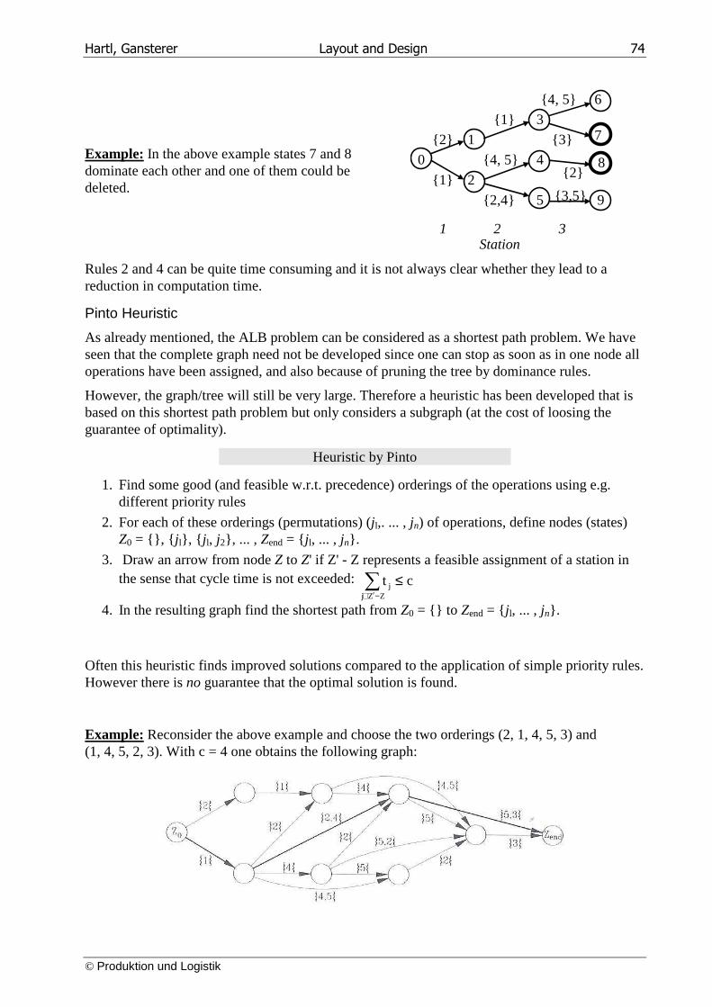
Hartl, Gansterer Layout and Design 74
© Produktion und Logistik
Example: In the above example states 7 and 8 dominate each other and one of them could be deleted.
{4, 5} 6
{1} 3
{2} 1 {3} 7
0 {4, 5} 4 8
{1} 2 {2}
{2,4} 5 {3,5} 9
1 2 3 Station
Rules 2 and 4 can be quite time consuming and it is not always clear whether they lead to a reduction in computation time.
Pinto Heuristic
As already mentioned, the ALB problem can be considered as a shortest path problem. We have seen that the complete graph need not be developed since one can stop as soon as in one node all operations have been assigned, and also because of pruning the tree by dominance rules.
However, the graph/tree will still be very large. Therefore a heuristic has been developed that is based on this shortest path problem but only considers a subgraph (at the cost of loosing the guarantee of optimality).
Heuristic by Pinto
1. Find some good (and feasible w.r.t. precedence) orderings of the operations using e.g. different priority rules
2. For each of these orderings (permutations) (j l,. ... , jn) of operations, define nodes (states) Z0 = {}, { j l}, { j l, j2}, ... , Zend = { j l, ... , jn}.
3. Draw an arrow from node Z to Z' if Z' - Z represents a feasible assignment of a station in the sense that cycle time is not exceeded: ∑
−′∈
≤ZZj
j ct
4. In the resulting graph find the shortest path from Z0 = {} to Zend = { j l, ... , jn}.
Often this heuristic finds improved solutions compared to the application of simple priority rules. However there is no guarantee that the optimal solution is found.
Example: Reconsider the above example and choose the two orderings (2, 1, 4, 5, 3) and (1, 4, 5, 2, 3). With c = 4 one obtains the following graph:
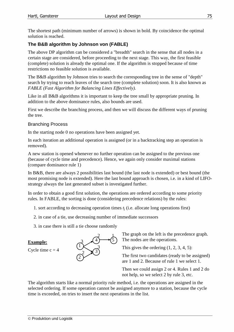
Hartl, Gansterer Layout and Design 75
© Produktion und Logistik
The shortest path (minimum number of arrows) is shown in bold. By coincidence the optimal solution is reached.
The B&B algorithm by Johnson von (FABLE)
The above DP algorithm can be considered a "breadth" search in the sense that all nodes in a certain stage are considered, before proceeding to the next stage. This way, the first feasible (complete) solution is already the optimal one. If the algorithm is stopped because of time restrictions no feasible solution is available.
The B&B algorithm by Johnson tries to search the corresponding tree in the sense of "depth" search by trying to reach leaves of the search tree (complete solution) soon. It is also known as FABLE (Fast Algorithm for Balancing Lines Effectively).
Like in all B&B algorithms it is important to keep the tree small by appropriate pruning. In addition to the above dominance rules, also bounds are used.
First we describe the branching process, and then we will discuss the different ways of pruning the tree.
Branching Process
In the starting node 0 no operations have been assigned yet.
In each iteration an additional operation is assigned (or in a backtracking step an operation is removed).
A new station is opened whenever no further operation can be assigned to the previous one (because of cycle time and precedence). Hence, we again only consider maximal stations (compare dominance rule 1)
In B&B, there are always 2 possibilities last bound (the last node is extended) or best bound (the most promising node is extended). Here the last bound approach is chosen, i.e. in a kind of LIFO-strategy always the last generated subset is investigated further.
In order to obtain a good first solution, the operations are ordered according to some priority rules. In FABLE, the sorting is done (considering precedence relations) by the rules:
1. sort according to decreasing operation times tj (i.e. allocate long operations first)
2. in case of a tie, use decreasing number of immediate successors
3. in case there is still a tie choose randomly
Example:
Cycle time c = 4
2 1 3 4 5 1 3 2 3 2
The graph on the left is the precedence graph. The nodes are the operations.
This gives the ordering (1, 2, 3, 4, 5):
The first two candidates (ready to be assigned) are 1 and 2. Because of rule 1 we select 1.
Then we could assign 2 or 4. Rules 1 and 2 do not help, so we select 2 by rule 3, etc.
The algorithm starts like a normal priority rule method, i.e. the operations are assigned in the selected ordering. If some operation cannot be assigned anymore to a station, because the cycle time is exceeded, on tries to insert the next operations in the list.
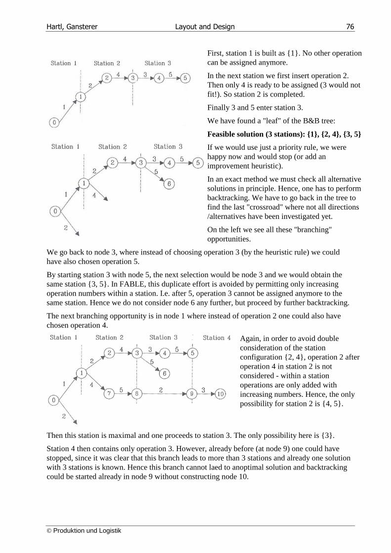
Hartl, Gansterer Layout and Design 76
© Produktion und Logistik
First, station 1 is built as {1}. No other operation can be assigned anymore.
In the next station we first insert operation 2. Then only 4 is ready to be assigned (3 would not fit!). So station 2 is completed.
Finally 3 and 5 enter station 3.
We have found a "leaf" of the B&B tree:
Feasible solution (3 stations): {1}, {2, 4}, {3, 5}
If we would use just a priority rule, we were happy now and would stop (or add an improvement heuristic).
In an exact method we must check all alternative solutions in principle. Hence, one has to perform backtracking. We have to go back in the tree to find the last "crossroad" where not all directions /alternatives have been investigated yet.
On the left we see all these "branching" opportunities.
We go back to node 3, where instead of choosing operation 3 (by the heuristic rule) we could have also chosen operation 5.
By starting station 3 with node 5, the next selection would be node 3 and we would obtain the same station {3, 5}. In FABLE, this duplicate effort is avoided by permitting only increasing operation numbers within a station. I.e. after 5, operation 3 cannot be assigned anymore to the same station. Hence we do not consider node 6 any further, but proceed by further backtracking.
The next branching opportunity is in node 1 where instead of operation 2 one could also have chosen operation 4.
Again, in order to avoid double consideration of the station configuration {2, 4}, operation 2 after operation 4 in station 2 is not considered - within a station operations are only added with increasing numbers. Hence, the only possibility for station 2 is {4, 5}.
Then this station is maximal and one proceeds to station 3. The only possibility here is {3}.
Station 4 then contains only operation 3. However, already before (at node 9) one could have stopped, since it was clear that this branch leads to more than 3 stations and already one solution with 3 stations is known. Hence this branch cannot laed to anoptimal solution and backtracking could be started already in node 9 without constructing node 10.
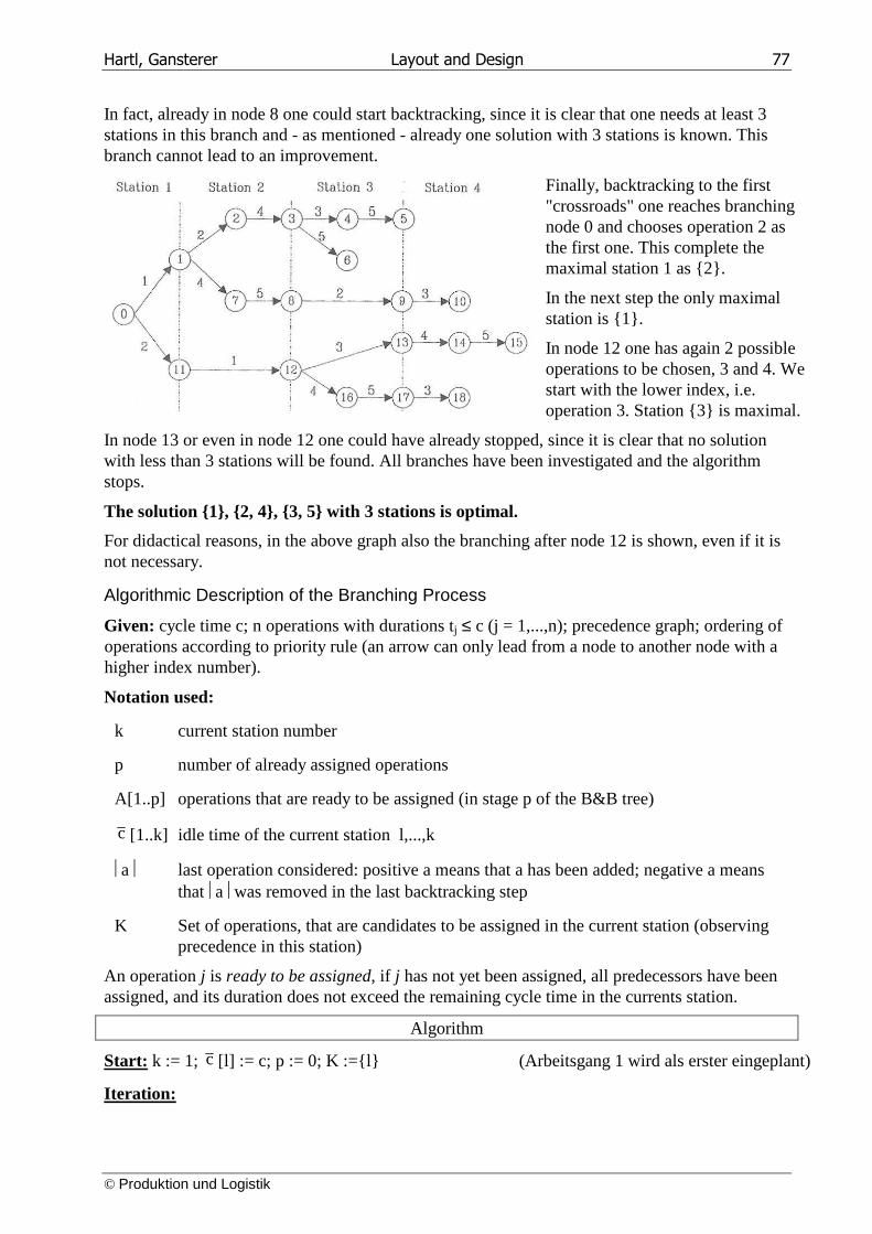
Hartl, Gansterer Layout and Design 77
© Produktion und Logistik
In fact, already in node 8 one could start backtracking, since it is clear that one needs at least 3 stations in this branch and - as mentioned - already one solution with 3 stations is known. This branch cannot lead to an improvement.
Finally, backtracking to the first "crossroads" one reaches branching node 0 and chooses operation 2 as the first one. This complete the maximal station 1 as {2}.
In the next step the only maximal station is {1}.
In node 12 one has again 2 possible operations to be chosen, 3 and 4. We start with the lower index, i.e. operation 3. Station {3} is maximal.
In node 13 or even in node 12 one could have already stopped, since it is clear that no solution with less than 3 stations will be found. All branches have been investigated and the algorithm stops.
The solution {1}, {2, 4}, {3, 5} with 3 stations is optimal.
For didactical reasons, in the above graph also the branching after node 12 is shown, even if it is not necessary.
Algorithmic Description of the Branching Process
Given: cycle time c; n operations with durations tj ≤ c (j = 1,...,n); precedence graph; ordering of operations according to priority rule (an arrow can only lead from a node to another node with a higher index number).
Notation used:
k current station number
p number of already assigned operations
A[1..p] operations that are ready to be assigned (in stage p of the B&B tree)
c [1..k] idle time of the current station l,...,k
a last operation considered: positive a means that a has been added; negative a means that a was removed in the last backtracking step
K Set of operations, that are candidates to be assigned in the current station (observing precedence in this station)
An operation j is ready to be assigned, if j has not yet been assigned, all predecessors have been assigned, and its duration does not exceed the remaining cycle time in the currents station.
Algorithm
Start: k := 1; c [l] := c; p := 0; K :={l} (Arbeitsgang 1 wird als erster eingeplant)
Iteration:
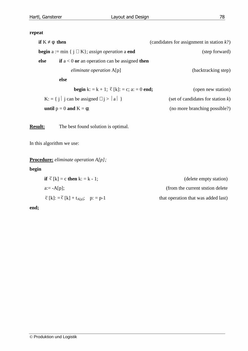
Hartl, Gansterer Layout and Design 78
© Produktion und Logistik
repeat
if K ≠ φ then (candidates for assignment in station k?)
begin a := min { j ∈ K}; assign operation a end (step forward)
else if a < 0 or an operation can be assigned then
eliminate operation A[p] (backtracking step)
else
begin k: = k + 1; c [k]: = c; a: = 0 end; (open new station)
K: = { j j can be assigned ∧ j > a } (set of candidates for station k)
until p = 0 and K = φ; (no more branching possible?)
Result: The best found solution is optimal.
In this algorithm we use:
Procedure: eliminate operation A[p];
begin
if c [k] = c then k: = k - 1; (delete empty station)
a:= -A[p]; (from the current ststion delete
c [k]: = c [k] + tA[p]; p: = p-1 that operation that was added last)
end;
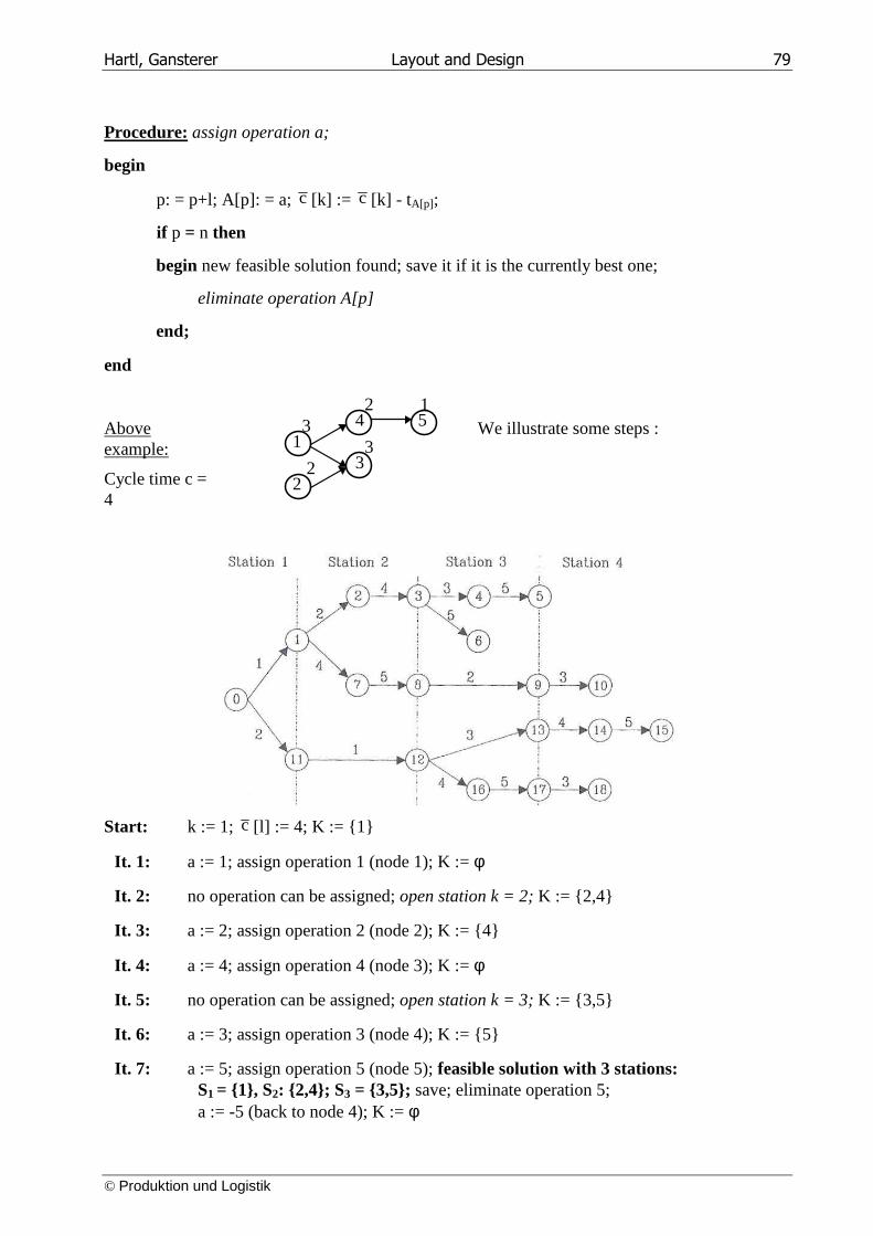
Hartl, Gansterer Layout and Design 79
© Produktion und Logistik
Procedure: assign operation a;
begin
p: = p+l; A[p]: = a; c [k] := c [k] - tA[p];
if p = n then
begin new feasible solution found; save it if it is the currently best one;
eliminate operation A[p]
end;
end
Above example:
Cycle time c = 4
2 1 3 4 51 3 2 32
We illustrate some steps :
Start: k := 1; c [l] := 4; K := {1}
It. 1: a := 1; assign operation 1 (node 1); K := φ
It. 2: no operation can be assigned; open station k = 2; K := {2,4}
It. 3: a := 2; assign operation 2 (node 2); K := {4}
It. 4: a := 4; assign operation 4 (node 3); K := φ
It. 5: no operation can be assigned; open station k = 3; K := {3,5}
It. 6: a := 3; assign operation 3 (node 4); K := {5}
It. 7: a := 5; assign operation 5 (node 5); feasible solution with 3 stations: S1 = {1}, S2: {2,4}; S3 = {3,5}; save; eliminate operation 5; a := -5 (back to node 4); K := φ
Hartl, Gansterer Layout and Design 80
© Produktion und Logistik
It. 8: a < 0; eliminate operation 3; a := 3 (back to node 3); K := {5}
It. 9: a := 5; assign operation 5 (node 6); K := φ
It. 10. operation 3 can be assigned; eliminate operation 5; a := -5 (back to node 3); K := φ (although 3 could be assigned, we do backtracking, since combination {3,5} in station 3 was already considered)
It. 11: operations 3 and 5 could be assigned; eliminate op. 4; a := -4 (back to node 2); K := φ
It. 12: operation 4 can be assigned; eliminate operation 2; a := -2 (back to node 1); K := {4}
It. 13: a := 4; assign operation 4 (node 7); K := {5}
It. 14: a: = 5; assign operation 5 (node 8); K := φ
It. 15: no operation can be assigned; open station k = 3; K := {2}
It. 16: a := 2; assign operation 2 (node 9); K := φ
It. 17: no operation can be assigned; open station 4; K := {3}
It. 18: a := 3; assign operation 3 (node 10); feasible solution with 4 stations: S1 = {1}; S2 = {4,5}; S3 = {2}; S4 = {3}; eliminate operation 3; a := -3 (back to node 9); K := φ
etc.
Fathoming of subproblems/branches in FABLE:
It is important to find ways to remove (delete, fathom) as many branches of the B&B tree in order to speed up the process. For that, one can use dominance rules (just like in DP) as well as bounds on the objective.
Here, we use Dominance Rules 1 and 2. Dominance rule 1 (maximal stations) is implicitely used in the algorithm; rule 2 must be slighty reformulated compared to FABLE.
Dominance Rule 2': A node of the tree can be deleted, if for the current maximal station Sk
holds:: There exists an operation h ∈ Sk and an operation j that has not yet been assigned such that N(h) ⊆ N(j) and th ≤ tj and c [k]- t j + th ≥ 0. If th = tj and N(h) = N(j) gilt, also j > h is required.
In the example node 8 is dominated by node 3, since there station 2 has more workload assgned and N(5) ⊆ N(2) gilt.
Also node 11 is dominated by node 1.
Dominance Rule 2´ can be applied in 2 steps. In a pre-processing step (before branching) all pairs if operations (h, j) are stored, that satisfy the fisrt two conditions (potential dominance).
Just before opening a new station one checks for each operation h whether it is dominated by another operation j ∈ K that is ready to be assigned. In this case we delete the node and start backtracking..
FABLE uses two more dominance rules:
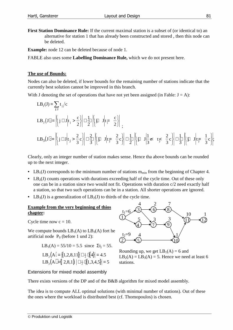
Hartl, Gansterer Layout and Design 81
© Produktion und Logistik
First Station Dominance Rule: If the current maximal station is a subset of (or identical to) an alternative for station 1 that has already been constructed and stored , then this node can be deleted.
Example: node 12 can be deleted because of node 1.
FABLE also uses some Labelling Dominance Rule, which we do not present here.
The use of Bounds:
Nodes can also be deleted, if lower bounds for the remaining number of stations indicate that the currently best solution cannot be improved in this branch.
With J denoting the set of operations that have not yet been assigned (in Fable: J = A):
∑∈
=Jj
j1 ct (J)LB
( )LB J : j J tc
2j J t
c
22 j j= ∈ >
+ ⋅ ∈ =
1
2 ;
( )LB J : j J t2
3c
2
3j J t
2
3c
1
2j J
1
3c t
2
3c
1
3j J t
1
3c3 j j j j= ∈ >
+ ⋅ ∈ =
+ ⋅ ∈ < <
+ ⋅ ∈ =
;
Clearly, only an integer number of station makes sense. Hence tha above bounds can be rounded up to the next integer.
• LB1(J) corresponds to the minimum number of stations mmin from the beginning of Chapter 4.
• LB2(J) counts operations with durations exceeding half of the cycle time. Out of these only one can be in a station since two would not fit. Operations with duration c/2 need exactly half a station, so that two such operations can be in a station. All shorter operations are ignored.
• LB3(J) is a generalization of LB2(J) to thirds of the cycle time.
Example from the very beginning of thios chapter:
Cycle time now c = 10.
We compute bounds LB1(A) to LB3(A) fort he artificial node P0 (before 1 und 2):
LB1(A) = 55/10 = 5.5 since Σtj = 55.
( ) { } { }( ) { } { } 51,3,4,52,8,11ALB
4.541,2,8,11ALB
21
3
21
2
=⋅+==⋅+=
t1=61
112
1011 3
9 37
78
26
43
54
..110
t2=92
45
Rounding up, we get LB1(A) = 6 and LB2(A) = LB3(A) = 5. Hence we need at least 6 stations.
Extensions for mixed model assembly
There exists versions of the DP and of the B&B algorithm for mixed model assembly.
The idea is to compute ALL optimal solutions (with minimal number of stations). Out of these the ones where the workload is distributed best (cf. Thomopoulos) is chosen.
Hartl, Gansterer Layout and Design 82
© Produktion und Logistik
In order to find all optimal solutions (not just one) all nodes that can also lead to a solution with the same number of stations must be kept. Above we only kept those where an improvement was possible. Hence the tree becomes larger and the computation times will increase.


