Page 1
MODULAR MULTI-SCALE ASSEMBLY SYSTEM FOR MEMS PACKAGING
by
RAKESH MURTHY
Presented to the Faculty of the Graduate School of
The University of Texas at Arlington in Partial Fulfillment
of the Requirements
for the Degree of
MASTER OF SCIENCE IN MECHANICAL ENGINEERING
THE UNIVERSITY OF TEXAS AT ARLINGTON
December 2005
Page 2
ii
ACKNOWLEDGEMENTS
With this degree, I feel one step closer to my goal. I wish to begin by thanking
my Mom, Dad and my Brother.
I would like to thank Dr. Raul Fernandez for his constant support and
encouragement shown in the past two years. I am indebted to Dr. Dan Popa for his
support and belief in my ability. I have seen tremendous improvements in my skills and
confidence under his supervision. I look forward to many more years of close
association with him. I would also like to thank Dr.Agonafer for his encouragement.
I cannot undermine the role played by Dr. Jeongsik Sin, Dr. Wo Ho Lee,
Dr. Heather Beardsley, Manoj Mittal, Abioudin Afosoro Amit Patil and Richard Bergs
for my success in the BMC project and subsequently in my thesis research.
Finally I wish to thank all my friends from UTA and in India.
November 11, 2005
Page 3
iii
ABSTRACT
MODULAR MULTI-SCALE ASSEMBLY SYSTEM
FOR MEMS PACKAGING
Publication No. ______
Rakesh Murthy, MS
The University of Texas at Arlington, 2005
Supervising Professor: Dr. Raul Fernandez
A multi-scale robotic assembly problem is approached here with focus on mechanical
design for precision positioning at the microscale. The assembly system is characterized
in terms of accuracy/repeatability and calibration via experiments. The MEMS
packaging requirements are studied from an assembly point of view. The tolerance
budget of the assembly ranges from 4 microns to 300 microns. The system components
include robots, microstages, end-effectors and fixtures that accomplish the assembly
tasks. Task assignment amongst this hardware has been accomplished based on
precision and dexterity availability. Various end-effectors and fixtures have been
designed for use with off-the-shelf hardware (robots and microstages) to develop a
coarse-fine positioning system. These end-effector and fixture designs are tested for
Page 4
iv
precision performance. The robots and the vision system are calibrated to an accuracy
of 11 microns or less. Inverse kinematics solutions for one of the robots have been
developed in order to position parts in the global coordinate frame. Conclusions have
been drawn with regard to implementation of calibration, fixturing, visual servoing or a
combination of these techniques to achieve assembly within the specified tolerance
budget as required by the target application. End-effector performance is improved by
tuning the PID gains of the controller such that tool oscillations are minimized.
Page 5
v
TABLE OF CONTENTS
ACKNOWLEDGEMENTS....................................................................................... ii
ABSTRACT .............................................................................................................. iii
LIST OF ILLUSTRATIONS…................................................................................. vii
LIST OF TABLES..................................................................................................... ix
Chapter
1. INTRODUCTION……… ............................................................................. 1
1.1 Motivation – Multi-Scale Assembly.................................................... 1
1.2 Problem Statement .............................................................................. 3
1.3 Approach……….. ............................................................................... 4
1.4 Accomplishments................................................................................ 6
1.5 Summary…………............................................................................. 9
2. BACKGROUND………............................................................................... 10
2.1 Microassembly…................................................................................ 10
2.2 Precision assembly.............................................................................. 13
2.3 Errors in Manipulators ........................................................................ 15
2.4 Modular/ Reconfigurable assembly system........................................ 16
2.5 Visual Servoing ............................................................................... 17
3. SYSTEM ARCHITECTURE ....................................................................... 19
3.1 Parts to be assembled .......................................................................... 19
Page 6
vi
3.2 Assembly Sequence ............................................................................ 21
3.3 Precision Requirements ...................................................................... 22
3.4 System Components ........................................................................... 25
3.5 End-Effector / Fixture Design… ........................................................ 29
4. SYSTEM ANALYSIS…............................................................................... 38
4.1 End-Effector Performance .................................................................. 38
4.2 Calibration………. ............................................................................. 48
4.3 PID gain tuning/Tool oscillations…………....................................... 60
4.4 Inverse Kinematics….. ....................................................................... 60
5. CONCLUSIONS AND FUTURE WORK.................................................... 63
REFERENCES… ...................................................................................................... 65
BIOGRAPHICAL INFORMATION......................................................................... 69
Page 7
vii
LIST OF ILLUSTRATIONS
1.1 MEMS package ................................................................................................... 3
1.2 Approach.............................................................................................................. 5
2.1 “Sticking effect” in microassembly ..................................................................... 12
2.2 Principles of RCC............................................................................................... 14
2.3 Picture of microfactory ....................................................................................... 16
3.1 Completed package.............................................................................................. 20
3.2 Exploded view of components to be assembled .................................................. 20
3.3 Package alignment ............................................................................................... 23
3.4 Tolerance budget description............................................................................... 23
3.5 RobotWorld ® setup............................................................................................ 25
3.6 Multi-scale mechanical setup .............................................................................. 26
3.7 Fine positioning system ....................................................................................... 27
3.8 Schematic diagram of supervisory control system .............................................. 28
3.9 RobotWorld setup shown with platen (translucent) ............................................ 29
3.10 Package gripper .................................................................................................. 30
3.11 Vacuum pick-up tool ......................................................................................... 31
3.12 Fiber gripper ...................................................................................................... 32
3.13 Tool rest fixtures................................................................................................ 33
3.14 Fiber insertion platform..................................................................................... 35
Page 8
viii
3.15 Plate holding fiber spool.................................................................................... 35
3.16 Fiber tilt experiment test-bed............................................................................. 36
3.17 Laser Fixture...................................................................................................... 37
4.1 Bulls eye diagram ................................................................................................ 38
4.2 Camera accuracy.................................................................................................. 40
4.3 CCD accuracy datapoints .................................................................................... .42
4.4 Camera robot repeatability datapoints ................................................................. 43
4.5 Robot repeatability............................................................................................... 44
4.6 Robot repeatability datapoints ............................................................................. 46
4.7 Four-axis robot accuracy ..................................................................................... 48
4.8 Assembly system coordinate frames ................................................................... 51
4.9 Camera/ robot calibration .................................................................................... 52
Page 9
ix
LIST OF TABLES
3.1 Tolerance budget ................................................................................................. 24
3.2 Fiber tilt data........................................................................................................ 37
4.1 CCD accuracy datapoints .................................................................................... 41
4.2 CCD accuracy error ............................................................................................. 41
4.3 Camera robot repeatability datapoints ................................................................ 42
4.4 Camera robot repeatability error table................................................................. 43
4.5 Robot repeatability datapoints ............................................................................ .45
4.6 Robot repeatability error table ............................................................................. 45
4.7 Robot accuracy datapoints................................................................................... 47
4.8 Robot acuracy error table..................................................................................... 47
4.9 Camera and pixel coordinates for grid................................................................. 56
4.10 Eight point calibration datapoints...................................................................... 57
4.11 Calibration Datapoints ....................................................................................... 58
4.12 Calibration Error ................................................................................................ 58
4.13 Twenty seven point calibration datapoints ........................................................ 59
Page 10
1
CHAPTER 1
INTRODUCTION
1.1 Motivation- Multi-Scale Assembly
The term “Multi-Scale” in robotics refers to assembly or manipulation
operations performed over a combination of scales like macro-meso-micro or meso-
micro-nano. The exact nature of this combination is more specific to the problem in
hand. Traditionally, the automation and robotics industries have dealt with challenges
encountered in working within the framework of a single scale (macro or meso). In the
past decade as micro and nano technologies have emerged and grown, several
approaches towards assembly and manipulation at these scales have been proposed. We
have microassembly techniques such as self-assembly and microrobotics that limit the
working scale to a single level and as a parallel approach which links traditional
domains to the newer domains we have multi-scale assembly.
The multi-scale approach can be used to distribute the assembly tasks into sub-
components that fall into different scale-levels by selecting the advantages offered at
each of these scales. The macro-meso-micro assembly technique offers a distinct
advantage of combining high accuracy over a large range of motion. Microoptics
packaging may involve manipulating meso/micro sized parts such as optical fibers
within a few microns tolerance on a MEMS die with the fibers being few feet long. This
being the case we have to use a multi-scale approach to complete the task.
Page 11
2
Many challenges are encountered while accomplishing a multi-scale assembly
process. Each of the scales have their inherent physics which may be distinct from the
corresponding hand-shaking scales. Volumetric forces such as gravity dominates the
meso scale manipulation while in the micro scale surface forces such as stiction and
electrostatic forces dominate.[1] Factors such as this have a significant influence over
mechanical design. Grippers and fixtures that make up the mechanical system have to
cater to variation in dominant forces. At the micro and nano scales, gripper free
manipulation is often preferred as opposed to the macro and meso scales where it is
inevitable to use direct contact with grippers for part handling. Also, systems used in
multi-scale solutions pose dynamic issues like vibrations which have a significant effect
on the corresponding smaller scales. As we scale down from the macro or meso to the
micro scales, there is a marked increase in required precision levels. Thus the challenge
lies in integrating the different scales and at the same time maintaining required
precision. The accuracy of robots used for handling and positioning macro and meso
components need be within the working range of micropositioning systems. For
example, an industrial robot used for die pick and place needs to be precise enough to
place the die within the field of view of a camera or within the working range of a
microstage on which a mating component, like a package is placed.
Research on microassembly techniques has been ongoing since the mid 1990’s.
Examples are advances made in microassembly using precision positioning stages,
custom built tweezers made from LIGA, and visual servoing at Sandia and UCBerkeley
[2], microscope based servoing with force feedback[3-5], microassembly system with a
Page 12
3
six-axis robot and tool changers at the Fraunhoffer Institute [6], microassembly system
using SMA microgrippers at EPFL [7], desktop microfactories in Japan, Europe and US
[8,9,10], modular microassembly system using for optical fiber arrays and other
microoptical components at RPI [1,11,12] and modular microassembly system based on
planar linear motor positioners at CMU [13]. The results presented in this thesis
describe on-going research effort in multi-scale assembly at the Automation and
Robotics Research Institute at UTA.
1.2 Problem Statement
A robotic assembly cell capable of macro-meso-micro level assembly needs to be
developed to accomplish MEMS die packaging used in Safe & Arm application
requiring shelf lives exceeding twenty five years [24].
Fig 1.1 MEMS Package
Page 13
4
End effectors and fixtures need to be designed and used with available robots to
complete the assembly operation within a tolerance budget. This assembly cell requires
to be capable of manipulating and positioning the package meso components with
typical dimensions of about an inch or less like the MEMS die or carrier within an
accuracy of a few microns. Macro components that require handling include fiber spool
plates (6in X 3in X ¼ in) with grooves holding optic fibers and an enclosure (2in X 2in
X 0.5in) to facilitate reducing gas environment during solder reflow.
Typical manipulation operations include
� Pick and place of package, die and performs from parts tray to the hotplate to
constitute what was called “die attach”.
� Optic fiber handling and insertion into package.
� Solder preform handling and laser positioning for soldering.
The objective of this research is to develop a multi-scale assembly platform that is
modular and reconfigurable. We must be able to readily reuse the assembly system
for a different application by changing end-effectors and fixtures.
.
1.3 Approach
For the problem statement stated above the following approach is outlined. This
forms the framework of this thesis research.
Page 14
5
Identify precision requirement
Identify precision and motion (degrees of freedom) of off-the-shelf hardware
Distribute tasks among these hardware
Design end effectors and fixtures
Test and improve design
Figure1.2 Approach
We begin by investigating the tolerance set offered by the assembly. The
tolerance required during positioning of every single component is studied. This is
compared to the precision and dexterity offered by off-the-shelf hardware (robots) and
the various assembly operations are delegated to these robots. Next, we design and
fabricate end-effectors and fixtures capable of handing the parts and test their
performance against assembly techniques such as calibration, fixturing and visual
servoing.
Page 15
6
1.4 Accomplishments
System Architecture: Motoman RobotWorld ® assembly platform is chosen as
the basis for developing the microassembly cell. It is a modular automation work cell
shared by multiple robots or pucks. The robots available for this work are a 4 axis open
loop puck (x,y,z and θ), a closed loop 3 axis puck(x,y,and z) and a 2 axis XY camera
puck (later modified as a 4 axis - XYZθ robot). The custom made fine positioning
system consists of x, y, z axis microstages from Thorlabs ® and a rotation stage from
Aerotech®. The assembly operations are listed and compared with the available
positioning resources to determine the operations to be assigned to every robot. This
decision is also made keeping in mind the need to separate the work volumes of the
robots in order to avoid collision.
The four-axis robot is assigned the task of pick and place of the package
components. As this requires the robot to handle four different end effectors, quick
change adaptors are chosen to switch this robot from one tool to another depending on
the operation in hand.
End-effector/Fixture design & fabrication: Vacuum pickup tools with
sufficient degrees of freedom are designed for MEMS die and perform pick and place.
Pneumatic grippers are designed for package pick and place, fiber insertion and
handling of macro components like fiber spool plates and reducing environment
enclosure. The three-axis robot is assigned the task of laser handling. Laser is one of
two methods used to reflow solder during bonding process in the package; the other
Page 16
7
technique used is a hot-plate. Fixtures necessary to support the Optical Imaging
Accessory from underneath the Z axis of the robot are designed and fabricated. A
platform that supports fiber insertion into the package and the reducing gas environment
enclosure has been designed and fabricated. This formed the fine-positioning system of
the assembly station.
Assembly system calibration/Accuracy tests: Calibration has been conducted
on the camera robot and the 4 axis puck with the vacuum pick-up tool The calibration is
also verified to be accurate within 11 microns. The acuracy is critical in implementing
calibration as an assembly technique. The camera is calibrated first. The die is picked
up by the 4 axis puck and brought under the camera. The CCD is focused to view a
specific feature on the die and that is saved as a template. Using machine vision
software, when the camera is moved to different locations (in global coordinate frame),
pixel readings related to the template feature are noted. Different positions of the
camera robot and the corresponding pixel locations are tabulated. Using these in the
kinematic equations of the camera, the transformation matrix relating the CCD to the
Robot is derived. This relates the CCD coordinate frame to the RobotWorld coordinate
frame. Next the robot is moved to different locations along different axis (x, y andθ).
For each position, the corresponding 4-axis robot location, camera location and CCD
pixel readings are noted. These, along with the CCD to Camera transformation matrix
are plugged into the 4-axis robot kinematic equations and solved to derive the
transformation matrix that relates the feature on the die to the global coordinate frame.
Next, the calibration routine followed for the robots is verified. The 4-axis robot is
Page 17
8
driven to a new location in the work volume. The camera is now moved to view the die.
This gives us a new location for the camera, robot and the corresponding pixel readings
for the template feature. Using the camera calibration equations we can now locate the
die in the RobotWorld coordinate frame. Next we use the robot calibration equations
and map the die to the RobotWorld coordinate frame. It is found that this location
matches in close proximity (within 11 micron error in X and Y) to the location derived
from the camera calibration.
Inverse kinematic equations need to be developed and used to provide a means
of referencing the parts in RobotWorld coordinate frame. For example, specific
features on the die that aid in alignment of die to package can be identified and then the
robot can be moved to a calculated orientation (using inverse kinematic equations) to
position the die inside the package.
The knowledge of the positioning accuracy and repeatability of the robots is
necessary to validate the design compatibility with tolerance budget offered by the
problem in hand. More-so when the 4 axis robot switches tools via the quick change
mechanism and parts are vacuum picked using the vacuum pickup tool. Experiments to
determine the accuracy and repeatability of the camera and four axis robots have been
conducted. Based on the calibration experiments and the accuracy/repeatability
experiments, certain design/assembly rules pertaining to the usage of fixturing or
calibration or visual servoing or their combination are implemented.
PID gain tuning is essential to minimize oscillations caused during part
handling. The end-effectors are offset from the center of the robot and these offsets
Page 18
9
cause oscillations during robot operation. Gain tuning is performed specific to the tool-
manipulator combination to minimize the effect of these oscillations.
1.5 Summary
A robotic assembly cell with multi-scale capability has been developed. Various
mechanical tools and fixtures have been designed, built and tested to suit a packaging
assignment. The vibrations that occur with these tools have been minimized by PID
tuning followed by accuracy tests, which have been conducted to determine the exact
positioning accuracy of the robots and vision system. Robot calibration has been
conducted and verified to an accuracy of 11 microns. An inverse kinematic solution has
been developed for the four-axis robot with die handling tool to accomplish die attach
within acceptable accuracy limits.
Page 19
10
CHAPTER 2
BACKGROUND
2.1 Microassembly
Microassembly deals with assembly of components whose dimensions lie
between the conventional macro-scale (>1mm) and the molecular scale (<1µm)[16]. It
involves positioning, orienting and assembling of microscale components into complex
microsystems. In short, microassembly can be defined as the assembly of objects with
microscale and/or mesoscale features under microscale tolerances. In the past decade
significant progress has been achieved in microassembly, gripping, handling,
positioning and bonding of parts with dimensions between a few microns to several
millimeters [3, 11, 13, 14, 15, 16]. Due to the small size of these components, fairly
specialized microgrippers, fixtures and positioning systems have been developed [17-
22].
Need: Current microsystems generally use monolithic designs in which all components
are fabricated in one (lengthy) sequential process [16]. In contrast to the more
standardized IC manufacturing, a feature of this manufacturing technology is the wide
variety of non-standard processes and materials that may be incompatible with each
other. These incompatibilities severely limit the manufacture of complex devices. The
goal of microassembly is to provide a means to achieve hybrid micro-scale devices of
high complexity. Manufacturing hybrid microsystems poses many unique challenges to
Page 20
11
fabrication, packaging and interconnection techniques. As an enabling technique,
assembly plays an essential role in addressing these challenges. The functions of
assembly in microsystems manufacturing are similar to those in conventional
macroscale manufacturing. However, in terms of manipulation, assembly in
microsystems manufacturing is significantly different from that in both microscale
manufacturing and IC manufacturing.
Challenges: Assembly of micro components is associated with high precision
requirements. There is a demand to work at a few micron part sizes or at a few micron
tolerance.
Mechanically, it is difficult to use grippers because of the interaction forces
between grippers and parts. Also, the absolute position of parts and tools are much more
difficult to measure for microassembly.
Scaling effects also pose a challenge. Most microassembly solutions employ
conventional assembly concepts scaled down to the microscale, though their
effectiveness diminishes as part dimensions shrink below 100µm [1]. For parts with
masses of several grams, the gravitational force will usually dominate adhesive forces,
and parts will drop when the gripper opens. For parts with size less than a millimeter,
the gravitational and inertial forces may become insignificant compared to adhesive
forces, which are generally proportional to surface area. When parts become very small,
adhesive forces can prevent release of part from the gripper.
Page 21
12
Classification: The techniques currently in use for microassembly are serial
microassembly and parallel Microassembly [16].
Fig 2.1 “sticking effect” in microassembly; (a), (b) approach, (c)Grasp, (d) Place, (e) Release
(a)
(b)
(c)
(d)
(e)
Page 22
13
In serial microassembly, parts are put together one-by-one according to the
traditional pick and place paradigm. Serial microassembly may include manual
assembly with tweezers and microscopes, visually based and teleopertaed
microassembly, use of high precision macroscopic robots and microgrippers.
Parallel microassembly involves multiple parts (identical or different design)
being assembled simultaneously. This can be either deterministic or stochastic. In the
deterministic category the relationship between part and its destination is known, while
in the stochastic category this relationship is random or unknown. The parts involved in
stochastic microassembly “self-assemble”. Some examples of the motive forces that
cause this self-assembly can be fluidic agitation and vibratory agitation.
2.2 Precision assembly
Passive, active or a combination of the two styles of compliance can be
incorporated into an assembly station to maintain a high level of precision. RCC
(Remote Center Compliance) is a passive compensation device. Misalignment during
assembly or operation can consist of lateral and angular errors. The errors can be due to
machine inaccuracy, fixturing tolerances or part vibrations. One was to compensate for
these positioning errors is to include compliance laterally and angularly, so as to allow
an assembly machine or robot to compensate for positioning error.
Principles of RCC: There are four basic stages for a part mating (assembly of a peg into
a hole). 1. Approach-this occurs when the robot brings the peg into the hole. 2. Chamfer
crossing- this happens when the robot initially starts to insert the peg. 3. One point
contact-the peg and the hole make side to side contact along their cylindrical side
Page 23
14
(a) (b)
(c) (d)
Fig 2.2 Principles of RCC, (a) approach, (b) chamfer crossing, (c) one point contact, (d)
two point contact
surfaces at one and only one point. 4. Two Point contact-the cylindrical surfaces of the
hole and the peg make contact at two points that join with a line drawn through the
longitudinal axis of the peg. The second type is the active method which uses a
controllable device to adjust actively during the parts mating process.
Page 24
15
2.3 Errors in Manipulators
Physical errors in manipulators can come from many sources. Some of them are
listed as follows [24]:
� Machining Errors: These errors are resulting from machining tolerances of the
individual mechanical components that are assembled to build the robot
� Assembly: These errors include linear and angular errors that are produced
during assembly of various components that are assembled to build the robot.
� Deflections: Errors can occur due to deflection of joints and links.
� Measurement and Control: Measurement, actuator and control errors will create
end effector positioning errors. The resolution of encoders and stepper motors
are example of such errors.
� Clearances: Backlash errors can occur in the motor gear box and in the
manipulator joints.
Errors are also repeatable and random [25]. Repeatable errors are errors whose
numerical value and sign are constant for each manipulator configuration. An example
of a repeatable error is an assembly error. Random errors are errors whose numerical
value and sign change unpredictably. An example of a random error is the error that
occurs due to backlash of an actuator gear train.
Page 25
16
2.4 Modular/ Reconfigurable assembly system
Microfactory: The microfactory as defined by the University of Tokyo, is a
means of achieving higher throughput with less space and reduced consumption of both
resources and energy via downsizing of production processes. Costs of microsystems is
dominated by production costs. Microfactories have the potential for reducing
production costs due to lower investment and less energy required. They carry the
advantage of producing at high speed due to lesser masses to be moved and shorter
distances to be traveled. They are also modular and can be modified easily to suit
changes in production type.
Minifactory: The SCARA (Selective Compliance Assembly Robot Arm)
manipulator is a popular choice for most automated assembly systems. However,
typical SCARA’s used in assembly have motion resolution and repeatabilities of 50 to
100 µm at best [13] which severly limits their use in high precision work. As a counter-
measure, an alternative robot configuration has been developed which provides the
same four degrees of freedom as a SCARA but which greatly ameliorates this problem.
Fig 2.3 Picture of Microfactory [13]
Page 26
17
The θ3 axis and the z axis of the SCARA are retained fixed in work-space. The θ1
and θ2 axes are discarded in favor of a X, Y stage robot called the “courier”. This robot
carries the subassembly. Moreover, this robot is implemented as a two axes linear motor
capable of traveling above a flat platen surface over a large workspace. An important
feature of this setup is that each of the 2 DOF robots can be an order of magnitude
smaller in size than a typical SCARA for assembling the same size product. This leads to
a large increase in achievable precision. The modularity of this system lies in the fact
that segments of a microfactory can be modified or extended with minimal or no impact
to the neighboring or any other part of the mini-factory.
2.5 Visual Servoing
Visual servoing is one of the approaches to the control of robot manipulators
that is based on visual perception of robot and workpiece location. More concretely,
visual servoing involves the use of one or more cameras and a computer vision system
to control the position of the robot's end-effector relative to the workpiece as required
by the task. It is a multi-disciplinary research area spanning computer vision, robotics,
kinematics, dynamics, control and real-time systems [26].
Visual servoing is an alternative to precise calibration. Traditionally, the
feedback provided to the assembly process by vision sensors has been incorporated into
the assembly process outside of the manipulator control loop. In visual servoing, we
place the vision sensor within the feedback loop of the manipulator. Using visual
feedback effectively in the control loop of an assembly process presents challenges
Page 27
18
quite different from those presented by othe feedback techniques like force feedback.
The large amount of data collected by a visual sensor causes the sampling rate to be
relatively small, and introduces large delays in the control loop. Since noise exists in
visual sensors and the sampling rate is low, robust feature trackers and control
algorithms must be used.
Page 28
19
CHAPTER 3
SYSTEM ARCHITECTURE
3.1 Parts to be assembled
The package in its assembled form is shown in the figure 3.1. The package
component’s sizes span over the meso and micro scales. Figure 3.2 shows an exploded
view of the package.
A Kovar ® carrier houses the entire package. The carrier is about 1’’ x 1’’ in
size and 0.25 inches in height. Kovar is an Iron based alloy with Cobalt and Nickel.
The MEMS die is a Deep Reactive Ion Etching (DRIE) Silicon On Insulator
(SOI) chip. The die is 12mm by 12mm in area. Fabricated on it are optical switches and
trenches in which optical fibers are inserted. The four trenches are 130 microns wide
and deep. The optical fibers are inserted through the carrier onto the die.
The optical fibers are 126 microns in diameter with Au coating at the tip. These
fibers are 2 feet long.
The preform that solders the die to the carrier is a Au-Sn eutectic alloy. It has a
thickness of 25 microns. This preform reflow is performed using a hot-plate.
The glass top chip sits on the MEMS die and is soldered onto it using Indium
solder pads deposited on the die. This has an area of 7.5 mm by 7.5 mm. The
functionality is to protect the MEMS die and to prevent the fiber from coming off the
die trench.
Page 29
20
Indium preforms solder the fiber onto the carrier. These preforms are cylindrical
in shape and have a diameter of 2mm and height of 4.5 mm. They are dropped into
holes in the carrier and soldered using laser in a reducing gas environment to prevent
their oxidation.
Fig 3.1 Completed package
Fig 3.2 Exploded view of components to be assembled [24]
MEMS die
Top Chip
Carrier
Fiber to package
preform
Optic fibers
Page 30
21
3.2 Assembly Sequence
The multi-scale assembly sequence followed to assemble the package
components is described here. Different components require different criteria for
assembly. Depending on the component type and the processes involved in attaching it
to the package body, specific robot end-effectors and fixtures need to be designed. The
overall packaging operation can be divided into two subsets of operations:
Die Attach: This is the sequence of operations followed to attach the MEMS die and the
top chip into the Kovar carrier. The stacking up of the components into the carrier is
performed on a hot plate. The following are the operations/manipulations involved.
a. The Kovar carrier is picked from the parts tray and placed on the
hotplate.
b. The 80Sn-20Au eutectic die preform is picked from the parts tray and
placed inside the package.
c. The MEMS die is picked from the parts tray, aligned to the carrier and
placed on the preform.
d. The top-chip is picked and placed on the die such that the preform pads
on the die are aligned to the matching pads on the top-chip.
This constitutes the “stack” of components inside the carrier. Following this is
the process of re-flow of the preform by turning on the hot-plate to a temperature of
350OC.
Page 31
22
Fiber Insertion and Attach: This involves optical fiber insertion into the package
followed by preform re-flow.
a. Following die-attach, the package is picked from the plate and placed
on the fiberspool plate (see section ) which constitutes the fine
manipulation system along with the microstages.
b. Optical fiber is inserted into the carrier, indium preform is dropped into
the carrier on the hole corresponding to the fiber.
c. A 60W Coherent® Quattro-FAP semiconductor diode laser is used to
melt indium that attaches the fiber onto the package. Operations ‘a’ , and
‘b’ are repeated for the other three fibers.
In addition to these, we have other manipulations related to fiber handling like
staging the fiber around the carrier before it can be inserted and providing a reducing
gas environment. All of these operations are described in greater detail in the
subsequent sections.
3.3 Precision Requirements
This section describes the tolerances permitted in positioning the components of
the package. Termed “Tolerance Budget”, these set of numbers constitute the basis for
the design and operation of the system. The gold coated optic fiber is 126 microns in
diameter and is inserted through the sidewall of the Kovar® package into a Deep
Reactive Ion Etching (DRIE) trench on the MEMS die. The fiber is constrained by the
trench in X,Y and by the die+ top chip in Z. The pitch and yaw are constrained by the
Page 32
23
feed through geometry in the package sidewall which has a tapering hole to feed the
fiber through it. The larger opening is 762 microns in diameter and the smaller opening
is 508 microns. The DRIE trench is 130 microns in width and is 130 microns deep. The
fiber is held in the trench by the top chip (not shown in figure 3.3)
The tolerance budget outlined in table 1 can be explained with reference to figure 3.4.
x
Y
z
θ
ϕ
Ψ
Carrier
Hole into
which
Indium is
dropped
MEMS Die
Fixture to
Support indium
preform
Fiber in
trench
Fig 3.3 Package alignment
Fig 3.4 Tolerance budget description;(a) package, (b) coordinate frame
(a) (b)
Page 33
24
The die to package tolerance is the tolerance offered when all the four fiber
trenches in the MEMS die are aligned to the corresponding four holes in the carrier. The
fiber to package tolerance is the tolerance permitted in inserting the optical fiber into the
outer hole on the Kovar carrier sidewall. The carrier has four tapering holes on its
sidewalls for inserting the fiber through them. The outer hole has a 762 micron
diameter. Fiber to trench tolerance is the clearance between the trench on the MEMS
die and the optical fiber. The optical fiber in constrained by the die on three sides and
the glass top chip on the top. The glass top chip has square pads which have to match
with the corresponding solder pads in the die. The tolerance offered in doing this is
referred to as the top chip to die tolerance in table 1. The Indium preforms are
cylindrical in shape. These preforms are dropped into the carrier that has four circular
openings perpendicular to the holes into which the fibers are inserted
. Table 3.1 Tolerance budget
∆X
∆Y
∆Z
∆θ (Yaw)
∆ϕ (Pitch)
∆ψ (Roll)
Die to Package 50 50 25 0.5 --- ---
Fiber to Package 300 300 186 0.859 0.859 ---
Fiber to Trench 04 04 25 0.2 --- ---
Top Chip to Die 50 50 25 0.22 --- ---
127 127 --- --- 8 8
tolerance in
microns and
degrees
In Preform to
Package
Page 34
25
3.4 System Components
The multi-scale assembly system comprises of many sub components which aid
coarse-fine motion and machine vision.. The multi-scale assembly cell comprises of an
automation workcell called RobotWorld® shown in figure 3.5.
The components are described here in detail
a) Coarse Positioning System: The workcell consists of multiple robots. These robots
are Cartesian with degrees of freedom ranging from 2 to 4.
Fig 3.5 RobotWorld® setup
Page 35
26
Fig 3.6 Multi-scale mechanical setup
1. Four axis (XYZθ) coarse manipulator robot
2. Four axis (XYZθ) coarse camera robot
3. Three axis (XYZ) fine manipulator robot
4. Optic Bread-Board
5. Three Axis (θXY) microstages (robot)
6. Parts Tray
7. Tool Rest
8. Hot Plate
1
2
3
5
6
7
8
4
Page 36
27
From figure 3.13, system (1) is A 4DOF (XYZθ) manipulator consisting of a
RM6210 RobotWorld® puck, which includes integrated I/O and pneumatic. (2) is a
4DOF (XYZθ) mobile camera module consisting of a 2DOF CM6200 RobotWorld®
puck base that carries a VZM 450 motorized zoom microscope, and a Thor Labs PT2-
Z6 stage (for autofocus). (3) is a 3DOF (XYZ) manipulator based on a RobotWorld®
TM6200GT closed-loop puck. (5) is a 3 DOF (θXY) manipulator based on an Aerotech
ART 315 rotational stage carrying two Thor Labs PT2-Z6 stages. Shown in figure 3.14,
this manipulator is a fine positioner, and is used as the holder platform for the package
during the fiber insertion and attachment processes.
(a)
Rotation Stage
Linear Stage X
Linear
Stage Y
Fiber
Insertion
Platform
Fig 3.7 Fine positioning system,(a) platform, (b)solid model
(b)
Page 37
28
The four axis robot (1) is configured to operate multiple tools with a Advanced
Robotics ® XC-1 quick change adaptor. Thus this robot operates the carrier gripper,
vacuum pickup tool, fiber gripper and the indium solder pickup tool. The three axis
robot (3) used for laser positioning with motion along X, Y and Z.
We use a custom supervisory controller implemented in Labview ™ running on
a Windows PC to integrate the assembly sequences, as shown in Figure 3.15. The PC
communicates via TCP-IP with the host RobotWorld® controller through ActiveX
commands. The supervisor communicates with the zoom camera via a National
Instruments IMAQ card and vision library, and with the microstages using the NI-
PCI7358 8-output motion control board and the NI Motion library.
Fig 3.8 Schematic diagram of supervisory control system
Supervisor (in Labview ™) High level commands Assembly and process sequence
RobotWorld (ORC) Low Level Motion Control (Pucks)
ActiveX
Motorized Microscope
NI IMAQ Card RS 232
Thorlabs, Aerotech stages
NI Motion Control
Coherent semiconductor laser
Process Tools Hot plate, grippers
RS 232 ActiveX
Page 38
29
3.5 End-Effector/Fixture Design
Various end effectors have been designed to be used in conjunction with the
robots. These end effectors have been designed to suit specific manipulation
requirements enlisted in section 3.2.
Generic Offset(s) Calculation: The RobotWorld ® pucks or robots occupy the available
working volume in an inverted Z fashion, upside down from the top (platen) to the optic
platform at the bottom. While systems like microstages, hotplate etc and fixtures like
parts tray, tool rests, etc are placed on the optic breadboard the robots reach from the
top to access them. We have designed tools incorporating this compensation in Z. Also,
when two pucks are coordinating an operation at the same time, we will have them
offset from the exact location of manipulation. For example when the camera robot is
viewing a die placement operation, the camera is right above the die. The tools which
carries the die is on the second robot which will have to operate from a distance in order
to avoid collision with the camera robot. Thus we need to design X, Y and Z offsets in
the tools. The exact value of these offsets is tool and operation specific.
Platen
Work
Volume
Puck
/Robot
Fig 3.9 RobotWorld setup shown with platen (translucent)
Page 39
30
The end effectors are described in the following section.
A. Carrier Gripper:
Functionality: This end-effector has been designed to handle the carrier. The carrier has
on four corners (shown below) holes that may be used for positioning and manipulation.
Operation: The gripper has two jaws that open and close pneumatically at an operating
pressure of 65 psi using RoboHand® RPLC-1 actuator. In their open position, the two
jaws slide into the diagonally opposing holes of the carrier (shown in figure 3.9).
Quick Change Adaptor
Pneumatic Actuator
Gripper Jaw
(b)
Figure 3.10 Package gripper (a) gripper, (b) carrier
(a)
Page 40
31
Other applications: This end-effector is also used to handle fiber-spool plates as well as
the enclosure used to produce reducing gas environment. This serves as a multi-purpose
end –effector. The four axis robot operates this tool via the Advanced Robotics XC-1 ®
quick change adaptor (shown in the figure 3.5).
B. Vacuum Pick-Up Tool
Functionality: This tool is used for pick & place operations of the MEMS die, the die to
carrier perform and the top chip.
Operation: The vacuum line runs through the quick change and connects to the probe. It
has the XC-1 ® quick change adaptor that facilitates usage with the four axis robot. A
three degree of freedom tilt stage as shown permits setting the orientation of the tip such
that the dies picked up are perfectly horizontal. This is critical to facilitate accurate pick
up and placing of the components.
3 dof tilt stage
Vacuum probe
Figure 3.11 Vacuum pick-up tool
Page 41
32
C. Fiber Gripper
Functionality: This tool is designed to grip the optic fiber while fiber insertion is carried
out on the microstages.
Operation: The fiber gripper consists of two opposing jaws that pneumatically open and
close. The fiber is pushed against a grove on one of the jaws by the second jaw.
Fig 3.12 Fiber gripper
D. Indium Pick-Up Tool:
Functionality: This vacuum operated tool is designed to pickup and drop cylindrical
indium performs from the parts tray into the carrier for fiber attach.
Operation: Much like the “Vacuum Pick-up Tool”, this end effector has a vacuum probe
with a tilt stage. It also has a quick change adaptor and is operated with the four axis
puck.
Page 42
33
E. Tool Rests: The tools described in the above sections are rested on the fixtures shown
while not in use by the robot (shown in figure). Each tool has the exact same set of
clearance holes that slide into the steel pins on the mating fixture plate. Currently in the
present setup we have four such fixtures in use for the four tools. The four axis robot
has the male quick change adaptor that mates with the female side of the quick change
adaptors on each of the tools.
Fig 3.13 Tool rest fixtures
A note on modularity: All the end effectors described here have similar quick change
adaptors attached in the same orientation and locations on the tools. The plates designed
for the end effectors are very similar to each other and are interchangeable from tool to
tool. The clearance holes on these tools which enable them to be placed on the tool rest
fixtures are located in the exact same locations on all tools. This adds to the mechanical
Locating
Pins
Page 43
34
modularity of the system. Any new tool designed requires minimal mechanical changes
in the tool design and no change in the fixtures used for tool resting.
F. Fiber insertion platform:
The fiber insertion and soldering operations are carried out by placing the package on a
set of microstages capable of high resolution linear and rotary motion. The fiber
insertion platform (shown in the figure) is a multi purpose design which serves the
following purposes:
a. Facilitates fiber insertion by locating carrier with respect to fiber spools on three
sides of the carrier.
b. Supports reducing gas enclosure while indium preforms reflow occurs.
c. Facilitates purging of reducing gas enclosure by supplying (N2 + H2) gases
internally.
d. Thermally isolates the microstages from the heat produced during laser
soldering of indium preforms.
Fiber handling with this platform: In the figure 3.9, the transparent parts are metal
plates that carry spools of fiber which are two feet long. They are wound on the circular
groove and presented at one end of the plate, where a rectangular slot is cut out to
accommodate the fiber gripper.
Page 44
35
Fig 3.15 Plate holding fiber spool
Kovar ®
Package
Fiber
insertion
platform
Fiber Spools
Fig 3.14 Fiber insertion platform
Page 45
36
Based on this design, the fiber is grasped about 2 to 2.5 inches away from the tip. This
causes the fiber to sag towards the tip that is inserted into the package. To determine the
exact nature of this problem, a testbed was setup as shown below.
The tilt stage helps in pre-setting a tilt on the fiber to compensate for the sagging that
occurs after lift. We start the experiment with no preset tilt much like how it is on the
fiber insertion platform. The following two images show the fiber tip when the fiber is
resting on the plate and after it is grasped/lifted for insertion.
The angle of this sag is measured to be within 1.04 degrees with the help of IMAQ ®
vision tool. This error is way above the tolerance for any of the fiber related assembly
operations (section 3.3). To minimize this angular error we use the tilt stage to incline
the fiber by the same angle in its rest position so that after pick-up the fiber tip droops
down to being horizontal. This experiment was repeated with different fiber samples
Plate carrying
fiber spools Tilt Stage
Optics with
camera
Fig 3.16 Fiber tilt experiment test-bed; (a) top view, (b) side view
(a)
(b)
Page 46
37
and using a preset tilt is found to reduce this pitch error to within 0.03 degrees which is
within the tolerance specified for the package (refer table 3.2)
Table 3.2 Fiber tilt data
SL NO Initial Angle -degrees
(before using tilt stage)
Final Angle - degrees
1 1.0373 0.0212
2 1.0012 0.0299
3 1.0154 0.0271
G. Laser Fixture
The laser support fixtures are attached to the closed loop (three axes) robot. The Optical
Imaging Accessory (OIA) is held in a fixture shown. The working distance of the laser
is about 3 cms. This means that the fixture should compensate for the z difference from
the bottom of the robot to about 2~4 cms from the focus point of the laser.
Laser Fixture
Fig3.17 Laser fixture
Page 47
38
CHAPTER 4
SYSTEM ANALYSIS
4.1 End-Effector Performance
Background definitions of robot precision:
a. Repeatability: The range of actual positions that a robot goes to when given the
same destination repeatedly.
b. Accuracy: The distance between the actual position in space to where the robot
should have ideally gone.
c. Resolution: The smallest increment which can be made in a given motion.
B
A
C
Figure 4.1 Bulls eye diagram;(a) good accuracy,(b)good repeatability,(c)ideal condition
Page 48
39
Bulls Eye Diagram: The bulls eye diagram shows three different cases of robot
positioning. In case A. the robot has poor repeatability but excellent accuracy. In case B
the robot has good repeatability but is highly inaccurate. In case C, the robot has good
accuracy and repeatability.
The tolerance budget for positioning of micro and mesoscale components is as
shown in section 3.3. The coarse positioning robots (four axis and camera pucks)
together with the fine positioning system should be able to work within this budget. In
this section we determine the positioning accuracy of the coarse positioning system.
Accuracy/Repeatability Experiments on RobotWorld: We have performed experiments
to determine the accuracy of any positioning system involving the usage of machine
vision and encoder feedback. A component is picked up by the robot and brought
underneath the camera with a pre-determined zoom level, and the camera is focussed on
it as shown in figure 4.2.. On the corresponding CCD image seen, one feature
convenient to be reliably used with machine vision is identified and saved as a template.
An example of a template is shown. Shown in the picture is a trench into which an optic
fiber is inserted. By repeated motions between two points, one of which is under the
camera, we can match the template to what is seen each time and thus determine the
accuracy.
Page 49
40
Fig 4.2 Camera accuracy;(a) setup,(b)CCD image
Camera robot accuracy and repeatability test: The camera robot consists of the XY
puck and the CCD with a motorized zoom microscope. In a setup such as this error
can creep in two ways. One way is through the image capture and processing system
(CCD + IMAQ® Machine vision software). This is determined by not moving
anything (camera robot or component) and repeatedly capturing images of the same
feature. The second source of error is the XY positioning system with the
mechanical fixturing involved. This error is determined by repeatedly moving the
camera robot between two points.
Type1: CCD accuracy (nothing moving). The above mentioned technique is
followed and the error of the first kind is determined. The data obtained are
tabulated. In the table shown Px and Py are the pixel readings for the CCD which
(a) (b)
Page 50
41
are transformed into RobotWorld coordinates X&Y using the transformation matrix
described in the calibration section.
Table 4.1 CCD accuracy datapoints
Sl No: Px Py X Y
1 360 157.5 99.6063 99.2035
2 361.121 158.399 99.604 99.2011
3 361.179 158.455 99.6039 99.201
4 361.727 159.175 99.6021 99.1999
5 361.778 159.291 99.6018 99.1998
6 362.735 159.273 99.6018 99.1976
7 361.875 159.395 99.6015 99.1996
8 362.81 159.532 99.6012 99.1974
9 362.104 159.635 99.6009 99.1991
10 362.082 160.334 99.5992 99.1993
From the table shown above, the following error table is generated.
Table 4.2 CCD accuracy error
X(mm) Y(mm)
-0.0023 -0.0024
-0.0024 -0.0025
-0.0042 -0.0036
-0.0045 -0.0037
-0.0045 -0.0059
-0.0048 -0.0039
-0.0051 -0.0061
-0.0054 -0.0044
-0.0071 -0.0042
From the data above the average errors in X and Y (Xm, Ym) can be found.
Xm= 4.48 microns
Ym= 4.08 microns
Standard deviation in X = 1.39
Standard deviation in Y= 1.21
Page 51
42
The edumnd optics zoom camera has a resolution of 3.33 microns per pixel at 4X zoom
and a FOV (field of view) of 2mm.
CCD accuracy
-7
-6
-5
-4
-3
-2
-1
0
-8 -7 -6 -5 -4 -3 -2 -1 0
error in X (micons)
err
or
in Y
(m
icro
ns)
Type2: Camera Robot Repeatability: Xc and Yc are the camera robot
coordinates in millimeters.
Table 4.3 Camera robot repeatability datapoints
Sl No: Xc Yc Px Py X Y
1 100 100 378.797 167.289 99.5818 99.1622
2 100 100 377.097 169.237 99.5769 99.1665
3 100 100 377.772 169.614 99.576 99.165
4 100 100 377.772 169.614 99.576 99.165
5 100 100 376.994 171.488 99.5713 99.1672
6 100 100 376.73 170.74 99.5731 99.1677
7 100 100 377.006 173.345 99.5666 99.1676
8 100 100 376.023 173.571 99.5661 99.1699
9 100 100 376.904 173.775 99.5656 99.1679
10 100 100 376.847 175.593 99.561 99.1684
Fig 4.3 CCD accuracy datapoints
Page 52
43
From the experimental data points in the table shown above the following error table is
generated.
X(mm) Y(mm)
-0.0049 0.0043
-0.0058 0.0028
-0.0058 0.0028
-0.0105 0.005
-0.0087 0.0055
-0.0152 0.0054
-0.0157 0.0077
-0.0162 0.0057
-0.0208 0.0062
From the data above the average errors in X and Y (Xm, Ym) can be found.
Xm= 11.5 microns
Ym= 5.04 microns
Standard deviation in X = 5.3
Standard deviation in Y= 1.48
Camera Robot Repeatability
0
1
2
3
4
5
6
7
8
9
-25 -20 -15 -10 -5 0
error in X (microns)
err
or
in Y
(m
icro
ns)
Table 4.4 Camera robot repeatability error table
Fig 4.4 Camera robot repeatability datapoints
Page 53
44
Robot Accuracy/Repeatability Test. Similar to the camera robot accuracy experiments,
we can determine the error involved in moving the four axis robot with an end-effector.
With focus on die-attach operation and considering the fact that most tools are used
with this robot via quick change, we find the accuracy of this robot with the vacuum
pick up tool that handles the die and the perform pick & place.
Type1: Point to Point Repeatability(without homing): The robot is moved between two
points one of which is monitored under the camera. While moving the robot between
these two points, the robot is not homed or reset.
(a)
(b)
Fig 4.5 Robot Repeatability ;(a)Point1,(b)Point2
Page 54
45
Point 1: X = 800mm
Y = 250.002mm
θ = 45.002 deg
Point 2: X = 679.251mm
Y = 167.656mm under the camera
θ = 10.824 deg
Table 4.5 Robot repeatability datapoints
Sl No: Px Py X(mm) Y(mm)
1 363.68 263.532 99.3412 99.2162
2 360.648 263.389 99.3415 99.2232
3 362.456 264.542 99.3386 99.2193
4 362.702 265.292 99.3368 99.2188
5 365.444 266.227 99.3344 99.2127
6 366.477 268.537 99.3287 99.2108
7 365.748 267.219 99.332 99.2122
8 365.696 267.511 99.3312 99.2124
9 367.419 267.364 99.3316 99.2084
10 366.478 268.521 99.3287 99.2108
Table 4.6 Robot repeatability error table:
X(mm) Y(mm)
0.0003 0.007
-0.0026 0.0031
-0.0044 0.0026
-0.0068 -0.0035
-0.0125 -0.0054
-0.0092 -0.004
-0.01 -0.0038
-0.0096 -0.0078
-0.0125 -0.0054
From the data above the average errors in X and Y (Xm, Ym) can be found.
Page 55
46
Xm= 7.48 microns
Ym= 1.91 microns
(Standard deviation in X = 4.29
Standard deviation in Y= 4.64)
The repeatability is 11.77 microns (sum of mean and standard deviation)
-10
-8
-6
-4
-2
0
2
4
6
8
-14 -12 -10 -8 -6 -4 -2 0 2
error in X (microns)
err
or
in Y
(m
icro
ns)
Type2: Home to point via parts tray (Accuracy Test): This experiment involves the
following sequence of operations. a) Robot Initializes. b) Moves to tool rest and
attaches to the vacuum pick-up tool via quick change. c) Moves to parts tray and picks
up the MEMS die. d) Moves to a location and places the die under the camera. This
sequence is repeated with the camera remaining in the exact same location. Each time
machine vision is used to detect the location of a specific feature on the die. We
Fig 4.6 Robot repeatability datapoints
Page 56
47
transform the pixel readings (Px and Py) into RobotWorld coordinates and measure the
error.
Operating Conditions are Zoom=4X; Robot Speed =5mm/s and acc=0.1mm/s2
The coordinates of the four axis robot underneath the camera are
X = 1306.016 mm
Y = 717.176 mm
θ = 50.019 deg
The data points for this experiment are
Table 4.7 Robot accuracy datapoints
Sl No: Px Py X (mm) Y(mm)
1 282.5 303 99.2425 99.4108
2 282.523 303.828 99.2904 99.411
3 282.56 303.042 99.2424 99.4608
4 284.433 303.053 99.29 99.4064
5 284.461 303.001 99.3425 99.4063
6 282.523 303.828 99.2404 99.411
Table 4.8 Robot accuracy error table:
X(mm) Y(mm)
0.0479 0.0002
-0.0001 0.05
0.0475 -0.0044
0.1 -0.0045
-0.0021 0.0002
Page 57
48
From the data above the average errors in X and Y (Xm, Ym) can be found.
Xm= 38.64 microns
Ym= 8.3 microns
Standard deviation in X = 23.7
Standard deviation in Y= 20.9
4-Axis Robot Accuracy
-10
0
10
20
30
40
50
60
-10 0 10 20 30 40 50 60
X
Y Series1
Figure 4.7 Four-axis robot accuracy
4.2 Calibration
The Multi-Scale assembly system consists of many different coordinate frames
that are attached with different components that make up the system (robots, tools,
fixtures and parts). Calibration is the procedure followed to represent all of these frames
with respect to a single global coordinate frame. Once calibrated, any operation can be
referenced with respect to this global coordinate frame. Robot calibration involves
Page 58
49
identifying a functional relationship between the joint transducer readings and the actual
workspace positions of the end effectors and using this to modify the robot control
software [26]. From this standpoint calibration can be defined as a process by which
robot accuracy is improved by modifying the robot positioning software rather than
changing or altering the design of the robot or the control system. Calibration is a
discrete event and is as such different from adaptive control where model identification
is carried out continuously and controller parameters are adjusted in accordance with
the identified changes.
In general calibration procedure consists of four steps. First step would be to
choose a suitable functional relationship. This could be referred to as a modeling step.
The second step would be to collect some data from the actual robot that relates the
input of the model to the output. This step is termed as the measurement step. The third
step is to use the data collected and mathematically calculate the unknown coefficients
in the model. The final step would be the implementation of the model into the inverse
kinematics for the robot.
The calibration method followed is the statistical calibration method which is an
alternative to the model based approach of calibration. In this method the manipulator is
commanded to many locations and the actual positions are recorded. From these two
sets of values (commanded position and actual position) a mapping can be derived by
doing a least squares fit on the data. We calibrate the robot to find out the relative
location of the parts in the RobotWorld platen coordinate frame (see figure 4.4). We
Page 59
50
have defined coordinate frames for all the different manipulators and for the part being
manipulated.
The statistical calibration method comes with the following advantages;
1) There is no concern over stability of parametric representations.
2) This method can take into consideration error sources which are not due to
geometric joint parameter errors, which leads to the possibility of this being a
more accurate means of calibration.
3) Once calibrated the computation of positions is faster
4) This method facilitates modularity of the assembly system. Any changes in tool
design can be easily accommodated in the calibration routine without focusing
much on the exact nature of the change.
The following are the disadvantages that are associated;
1) We need to ensure that many locations are used to calibrate; so the process can
be more tedious to begin with.
2) Little insight is given to the source of errors.
We find the transformation between the four axis manipulator coordinate system,
the local coordinate frame on the MEMS die and the four axis camera robot coordinate
frame. Finding this transformation reduces to a parameter identification problem for
several unknown coefficients. A schematic diagram of the relative position of several
local/global coordinate frames is shown in the figure here.
Page 60
51
Calibration Routine for RobotWorld: As shown in the figure 4.5, consider the case
when the camera is viewing a particular feature on the MEMS die on the four axis
robot. For example, this feature could be the centric of a DRIE trench on the die. Let
Xc, Yc, Zc be the joint coordinates of camera, Xo, Yo, Zo, θo be the joint coordinates
for four axis robot, and Xp, Yp, Zp be the coordinates of the point in the platen
coordinate frame.
Z
X
Y
4 axis puck
(Xo,Yo,Zo,θo)
3 axis puck (laser)
camera puck
(Xc,Yc,Zc)
Platen global
coordinate frame
Fine manipulation
system (Xf,Yf,Zf,θf)
MEMS Die Frame
(XP,YP,ZP,)
Fig 4.8 Assembly system coordinate frames
Page 61
52
Fig 4.9 Camera/robot calibration
Camera Calibration
Experimental Procedure:
(a) Identify the die feature to be used (with which the die coordinate frame will be
attached to)
(b) Move the camera to produce a grid of pixel coordinates (Pxi, Pyi)
(c) Record camera coordinates corresponding to pixel coordinates (Xci, Yci)
The platen (world) coordinates of the die (die feature) is given by
Zo
Zp
Zc
Xp Yp
Yo
Xo
Xc
Yc
+
=
yi
xi
ci
ci
p
p
p
pR
Y
X
Y
X1
…………. (1)
Page 62
53
For repeated readings, the (Xp, Yp) coordinates remain the same. Hence
……………..(2)
The above equation can be re-written as
…………....(3)
For ‘n+1’ trials; the above equation can be extended to
…….…….(4)
Re-writing the above equation,
…………..(5)
Unknowns are r11, r12, r21, r22.
∆
∆+
∆
∆=
yi
xi
ci
ci
p
pR
Y
X10
∆
∆−=
∆∆
∆∆
ci
ci
yi
yixi
Y
X
r
r
r
r
ppi
pp
22
21
12
11
00
00
∆
∆
∆
∆
∆
∆
−=
∆∆
∆∆
∆∆
∆∆
∆∆
∆∆
cN
cN
c
c
c
c
yNxN
yNxN
yx
yx
yx
yx
Y
X
Y
X
Y
X
r
r
r
r
pp
pp
pp
pp
pp
pp
MMMMM
2
2
1
1
22
21
12
11
22
22
11
11
00
00
00
00
00
00
[ ] [ ]v
r
r
r
r
w =
22
21
12
11
Page 63
54
We can solve this as a least squares fit on the data known using the pseudo-inverse
method. Thus we can map the die in the world coordinate frame. The identification of
the R matrix thus completes the calibration of the camera robot.
5 DOF manipulator calibration:
…………. (6)
‘OTN’ is the transformation matrix that relates the CCD pixel coordinate frame to the
robot coordinate frame. It accounts for rotation and scaling. ‘k1’ and ‘k2’ are the
translation factors.
Comparing this equation with equation(1),
……….. (7)
Pxinint and Pyinit are the first set of pixel coordinates as seen by the CCD. The
transformation matrix ‘OTN’ is represented by rotation matrix R and translation matrix
T. This rotation matrix is further represented in terms of R(θi) which is the subsequest
rotations involved.
+
+
=
1
)(T
0
2
1
11
0yinit
xinit
N P
P
k
k
Yo
Xo
Yp
Xp
θ
+
+
=
110
0
2
1
11
yinit
xinit
P
PTR
k
k
Yo
Xo
Yp
Xp
+
=
11
1 yinit
xinit
c
c
P
P
RY
X
Page 64
55
[ ]
−
−
+
=
Pyinit
PxinitRR
Yoi
Xoi
Pyi
PxiR
Yc
Xc
t
t
k
k
RI ii 1)(1
2
1
2
1
)(2 θθ
=
),,(
....
....
....
)2,2,2(
)1,1,1(
2
1
2
1
)(
.....
.....
.....
)(
)(
2
1
22
11
nYonXonv
YoXov
YoXov
t
t
k
k
nRI
RI
RI
nn θ
θ
θ
θ
θ
θ
+
+
+
=
+
+
+
=
+
2
1
1
)(1).(2
11
110
1
10
0)(
0
2
1
1110
01
1
t
tR
P
PRR
k
k
Y
X
P
PR
Yc
Xc
P
PTRR
k
k
Yo
Xo
P
PR
Yc
Xc
iyinit
xiniti
oi
oi
yi
xi
yinit
xinit
yinit
xinit
θθ
θ
…………. (8)
…………. (9)
…………. (10)
…………. (11)
Page 65
56
implies that the unknown matrix is given by
2
1
2
1
t
t
k
k
using the pseudo inverse function (least squares method) we can compute this matrix.
A Matlab® code is written and used to solve for the above unknowns using least square
fit. This completes the calibration procedure required.
Calibration Implementation: The calibration procedure described above is implemented
with the following details.
Step1: Camera Calibration
The operating conditions are as follows; Zoom=4X, Robot speed=10mm/s and
robot acceleration= 0.1mm/s2.
Table 4.9 Camera and pixel coordinates for grid
SL NO Xc-mm Yc-mm Px Py
1 100 100 421 221.5
2 99.25 100 428.116 374.431
3 99.75 100 423.271 273.455
4 99.75 100.25 372.772 272.852
5 99.25 100.25 377.798 373.624
6 100 100.25 370.693 223.823
7 100 100.5 314.765 222.369
8 99.75 100.5 315.88 271.935
9 99.25 100.5 321.164 372.673
…………. (12)
Page 66
57
For the grid shown above, the camera calibration results in the following
transformation matrix;
0.0001 0.0050
R1 =
0.0047 -0.0002
Step 2a: Robot Calibration (8 point calibration)
Operating Conditions
Robot Speed 5 mm/s
Acceleration 0.1mm/s2
All dimensions in mm
Table 4.10 Eight point calibration datapoints
SL NO variable Xo Yo θ −deg Px Py Xc Yc
1 599.021 305.327 77.498 421.634 222.729 100 100
2 x 599.493 305.327 77.498 425.685 325.611 100 100
3 y 599.493 304.751 77.498 308.367 323.351 100 100
4 θ 599.493 304.751 77.14 396.221 161.525 100 100
5 x,θ 599.153 304.751 77.752 245.757 368.669 100 100
6 x,y 598.499 306.001 77.746 497.827 235.384 100 100
7 y,θ 598.499 305.002 77.453 366.04 105.449 100 100
8 x.y,θ 599.743 304 77.002 282.732 155.685 100 100
The transformation matrix that results from the calibration procedure followed is
k1 -421.5726
k2 -77.2245
=
t1 -77.4068
t2 -128.0874
Page 67
58
Calibration Verification:
Table 4.11 Calibration Datapoints
SL NO Xo Yo θ Px Py Xc Yc
1 600 304 77.008 283.805 208.689 100 100
2 600 305 77.349 402.152 361.555 100 100
3 600 304.5 77.352 236.235 211.35 100.75 100.25
4 600.5 304.25 77.358 395.355 212.395 101.25 99.25
For the data points shown above, the following errors are obtained from the calibration
equations;
Table 4.12 Calibration Error
ErrorX ErrorY
5.4083 13.8928
4.2309 -6.6493
20.4007 2.831
-5.2499 6.7048
The eight point calibration technique yields a LSE residue of 20.4 microns.
Since we require that the residue be within the sum of repeatability of four axis puck +
repeatability of camera puck, which is 11.77 + 5.87=17.64 microns, the increase the
grid size used for robot calibration such that the variance is reduced below the threshold
of 17.64 microns. So we next try the 27 point calibration where in we form a 3X3X3
grid of variants (X, Y, and Theta).
Step2b. 27 Point Calibration: For similar operating conditions, the following datapoints
are collected.
Page 68
59
Table 4.13 Twenty seven point calibration datapoints
SL NO Xo Yo θ Px Py Xc(mm) Yc(mm)
1 679 168 11.002 272.5 135.5 104.9 102.569
2 679 168 10.9 387.236 141.386 104.9 102.569
3 679 168 10.8 488.792 147.48 104.9 102.569
4 679 167.751 11.002 175.517 138.722 104.9 102.569
5 679 167.751 10.894 283.302 146.328 104.9 102.569
6 679 167.751 10.811 389.359 153.283 104.9 102.569
7 679 167.65 11.002 137.715 146.337 104.9 102.569
8 679 167.65 10.9 245.211 151.448 104.9 102.569
9 679 167.65 10.83 322.381 157.433 104.9 102.569
10 679.249 167.999 11.008 297.602 244.431 104.9 102.569
11 679.249 167.999 10.9 402.766 250.562 104.9 102.569
12 679.249 167.999 10.83 472.389 247.22 104.9 102.569
13 679.249 167.751 11.002 190.481 239.658 104.9 102.569
14 679.249 167.751 10.9 301.101 247.606 104.9 102.569
15 679.249 167.751 10.843 367.341 252.269 104.9 102.569
16 679.249 167.653 11.008 150.936 243.553 104.9 102.569
17 679.249 167.653 10.9 261.697 250.412 104.9 102.569
18 679.249 167.653 10.83 332.53 255.21 104.9 102.569
19 679.499 168 11.002 301.592 350.484 104.9 102.569
20 679.499 168 10.9 417.548 358.339 104.9 102.569
21 679.499 168 10.83 490.274 363.324 104.9 102.569
22 679.499 167.751 11.002 200.452 355.724 104.9 102.569
23 679.499 167.751 10.894 316.618 363.39 104.9 102.569
24 679.499 167.751 10.83 389.438 368.304 104.9 102.569
25 679.499 167.656 11.008 174.625 358.393 104.9 102.569
26 679.499 167.656 10.9 279.353 365.61 104.9 102.569
27 679.499 167.656 10.83 350.634 370.258 104.9 102.569
This procedure yields a LSE residue of about 11 microns which is well below
the threshold variance figure of 17.64 microns set by the camera and the four axis
manipulator. With reference to the tolerance budget explained in section 3.3, this
calibration technique can be employed for the die to package assembly, Top Chip to Die
assembly and the Indium Preform to package assembly.
Page 69
60
The decision to employ calibration, fixturing or visual servoing can be based on
the following design rules
a. Fixtures can be used to locate objects in the assembly only when the
manipulator accuracy is smaller than the required part or feature tolerance.
b. Calibration can be used to locate objects in the workspace only if the
repeatability of the manipulator is smaller than the tolerance required.
c. Visual Servoing on the relative position between parts and tools can be used
only if the resolution of the manipulator is smaller than the tolerance required
4.3 PID gain tuning/Tool oscillations
The PID gain values of the controller are tuned to minimize the effect of
oscillations. The PID values are changes and the tool performance is observed under the
zoom microscope. This way the values are optimized. Gain tuning is particularly
important when the tools include high inertia and offsets. Also, gain tuning is performed
for all the tools with the robot that handle them.
4.4 Inverse Kinematics
Forward Kinematics (or direct kinematics) is the process of computing the
position and orientation of the tool relative to the global coordinate frame given the
joint angles of the manipulator. A greater challenge is to work a suitable set of values
for the robot joints to achieve a required tool position. This procedure is called Inverse
Kinematics.
Page 70
61
So far we have worked towards determining the accuracy and repeatability of
the positioning systems and towards expressing the various coordinate frames with
respect to the platen coordinate frame. We have also determined that the four axis robot
with the vacuum pick-up tool can be calibrated within the tolerance limit required for
die-attach. Next, we need to implement calibration such that using the zoom microscope
and the four axis robot (at the appropriate joint angles) accomplish die attach.
We use constrained least square solution to numerically calculate the pose of the
robot necessary to align the MEMS die to the package as follows:
1. We first image the location of the fiber feedthroughs on a Kovar carrier package.
We use the NI IMAQ library to compute the position of a point situated in the center
of three of the fiber feedthrough (one on each side of the package). These locations
are computed using the COARSE-2 calibration data to be at global coordinates
(Xpj, Ypj, Zpj), where 1≤j≤3.
2. We then present a MEMS die to the camera puck and we image the three
corresponding points in the center of the DRIE trenches. In pixel coordinates, these
points are at (Pxij, Pyij) initial coordinates.
3. We then solve the constrained LSE problem to find the joint coordinates of the
COARSE-2 manipulator that minimizes the error vector represented by the length
difference between points on the die and points on the package expressed in global
coordinates. We want to find Xo, Yo, and θo that minimize:
Page 71
62
2
2
13
1
1
2
1
,,)))(((min
+
−
−
−
∑
= t
t
p
pMR
k
k
Y
X
Y
X
j yij
xij
o
o
o
pj
pj
YX ooo
θθ
−=
)cos()sin(
)sin()cos()(
oo
oo
oRθθ
θθθ ,
by assigning )sin(),cos(,, 4321 oooo zzYzXz θθ ==== , we can reduce the inverse
kinematics problem to the following constrained LSE:
23
1 2
1
4
3
12
21
2
1
1
,,,)(min
24
23
4321
∑=
=+
−
−+
j j
j
jj
jj
zz
zzzz v
v
z
z
cc
cc
z
z
where C1j, C2j, V1j, and V2j are coefficients depending on calibrated kinematics and
feature locations in pixel coordinates. This constrained LSE has an exact solution that
can be found using Lagrange multipliers and the eigenvalue of a residual matrix.
However, during our die-package attach experiments we used a numerical solution
instead, based on the LSQNONLIN function of MATLAB.
…………. (12)
Page 72
63
CHAPTER 5
CONCLUSIONS AND FUTURE WORK
A robotic assembly cell with multi-scale capability has been developed to
perform a packaging assignment. The tolerance budget of the package has been studied.
Various mechanical tools and fixtures have been designed, built and tested , followed
by repeatability tests, which have been conducted to determine the exact positioning
accuracy of the robots and vision system. Calibration has been implemented to work
within the required tolerances. The four-axis robot accuracy is repeatable within 8
microns with the vacuum pickup tool and the vision system accuracy is 11.5 microns.
Statistical calibration results in variance being limited to 11 microns. Based on the
accuracy, repeatability and calibration experiments, we conclude that for die attach,
calibration is to be implemented and fixturing alone is not sufficient. For fiber insertion,
we visual servoing is the suggested technique to be followed. An inverse kinematics
solution has been developed for the four-axis robot with die handling tool to accomplish
die attach within acceptable accuracy limits.
This work can be continued to implement visual servoing for applications that
demand higher precision such as the fiber insertion into the trench within a tolerance of
4 microns. Also, statistical calibration needs to be further studied with regards to
optimizing the number of datapoints required to calibrate any given system. Also,
reformulation of the assembly sequencer using a discrete event controller (DEC)
Page 73
64
framework can be implemented. The mechanical design of the tools can be improved to
better suit the application and also to suit modularity need.
Page 74
65
REFERENCES
1. “Micro and Meso Scale Robotic Assembly”, Dan O. Popa and Harry E. Stephanou,
Center for Automation Technologies, Rensselaer Polytechnic Institute, Troy, New
York, USA
2. Feddema, J.T. Simon, R.W. , “Visual servoing and CAD-driven microassembly,” in
Robotics & Automation Magazine, Vol. 5, Issue 4, pp. 18-24, Dec. 1998.
3. Y. Zhou, B.J. Nelson, B. Vikramaditya, “Fusing Force and Vision Feedback for
Micromanipulation,” in Proc. of IEEE Conf. On Robotics and Automation (ICRA
’98), Leuven, Belgium, 1998
4. Y. Ge, J.A. Gaines, B.J. Nelson, “Open-structure reconfigurable experimental work-
station for fast and reliable microassembly,” in SPIE Proc. Microrobotics and
Microassembly II, Boston, MA, Nov. 2000, pp.21-32.
5. S.J. Ralis, B. Vikramaditya, B. J. Nelson, “Micropositioning of a Weakly Calibrated
Microassembly System Using Coarse-to-Fine Visual Servoing Strategies,” in IEEE
Transactions on Electronics Packaging Manufacturing, Vol 23, No.2, April 2000.
6. R.Eberhardt, T. Scheller, et., al., “Automated assembly of microoptical components,”
SPIE Proc. Microrobotics and Mycrosystem Fabrication, vol 3202, pp. 117-127,
Pittsburgh, USA, 1997
Page 75
66
7. Bleuler, H., Clavel, R., Breguet, J. M., Langen, H., & Pernette, E., “Issues in
precision motion control and microhandling,” In IEEE proceedings of ICRA, San
Francisco, CA, (pp. 959–964).
8. H. Bleuler, J.-M. Breguet, “Microfactory and Microrobotics Activities in Europe”, in
International Workshop on Micro-Factory (IWMF), Tsukuba, Japan, 1998.
9. T.Hirano, K. Furata, “Micromachine technology trends in microfactory,” in
International Workshop on Micro-Factory (IWMF), Minneapolis, Sept 2002
10. R. Hollis, J. Gowdy, “Miniature Factories for Precision Assembly,” in Proc. Int’l
Workshop on Micro-Factories, Tsukuba, Japan, December 7-8, 1998.
11. D.O. Popa, B.H. Kang, J. Sin, “Reconfigurable Microassembly System for
Photonics Applications,” in Proc. IEEE Conf. on Robotics and Automation,
Washington, D.C., 2002
12. D.O. Popa, et., al., “Dynamic Modeling and Open-Loop Control Of Thermal
Bimorph MEMS Actuators,” in Proc. IEEE Conf. on Robotics and Automation,
Taipei, Taiwan, 2003.
13. A.A. Rizzi, J. Gowdy, R.L. Hollis, “Agile assembly architecture: an agent based
approach to modular precision assembly systems,” in Proc. of 1997 IEEE
International Conference on Robotics and Automation, Volume: 2 , 20-25 April
1997, Pages:1511 – 1516
14. M.B. Cohn, et.,al., “Microassembly Technologies for MEMS,” SPIE
Micromachining and Microfabrication, Santa Clara, CA (September 1998
Page 76
67
15. S. Fatikow , J. Seyfried1 , St. Fahlbusch1 , A. Buerkle1 and F. Schmoeckel1 , “A
Flexible Microrobot-Based Microassembly Station,” in Journal of Intelligent and
Robotic Systems, Vol 27, No. 1-2, January 2000
16. K. Goldberg, K.F. Bohringer, R. Fearing, “MicroAssembly,” in Handbook of
Industrial Robotics, 2nd Edition, edited by S. Nof. John Wiley and Sons, 1999. pp
1045-1066
17. Y. Bellouard, “Microrobotics, Microdevices Based on Shape-Memory Alloys,” in
Encyclopedia of Smart Materials, Wiley, pp. 620-644, 2002
18. M. Mikawa, “Visual Servoing for Micro Mass Axis Alignment Device,” in Proc. of
IEEE/RSJ International Conference on Intelligent Robots and Systems (IROS),
1996, pp.1091-1096.
19. N. Isam N. Tahhan, Yan Zhuang, K.F. Bohringer, K.S.J. Pister, K. Goldberg,
“MEMS Fixtures for Handling and Assembly of Microparts,” SPIE's 1999
Symposium on Micromachining and Microfabrication, Santa Clara, California.
September, 1999.
20. O. T. Strand, M. E. Lowry, “Automated Fiber Pigtailing Technology,” Electronic
Components and Technology Conference, 1994, pp.1000-1003.
21. C. R. Witham, “Fiber-Optic Pigtail Assembly and Attachment Alignment Shift
Using a Low-Cost Robotic Platform,” Electronic Components and Technology
Conf., 2000, pp21-25.
22. S. Jang, “Automation Manufacturing Systems Technology for Opto-electronic
Device Packaging,” Electronic Components and Technology Conf., 2000, pp.10-14.
Page 77
68
23. D.O. Popa, M. Deeds, et. al., “ Automated Assembly and Hermetic Packaging of
MOEMS for Applications Requiring Extended Self-Lives,” in Proc. of ASME
IMECE, November 5-11, 2005
24. C. Mavroids, et., al., “ A Systematic Error Analysis of Robotic Manipulators:
Application to a High Performance Medical Robot”, Proceedings of the 1997
International Conference in Robotics and Automation, Albuquerque, NM, April,
1997.
25. Slocum A., “Precision Machine Design”., Englewood Cliffs 1992
26. Brad Nelson et.,al., “Visual Servoing for Robotic Assembly”, in Visual Servoing-
Real-Time Control of Robot Manipulators Based on Visual Sensory Feedback, ed.
K.Hashimoto, World Scientific Publishing Co. Pte. Ltd., River Edge, NJ, pp. 139-
164, 1993.
Page 78
69
BIOGRAPHICAL INFORMATION
Rakesh Murthy was awarded a Bachelor’s degree in Mechanical Engineering
from Rashtreeya Vidhyalaya College of Engineering, Bangalore, India in 2002 and a
Master’s degree in Mechanical Engineering from the University of Texas at Arlington
in 2005. He is currently pursuing PhD in Electrical Engineering at the University of
Texas at Arlington. He can be contacted at the following email address:
[email protected]


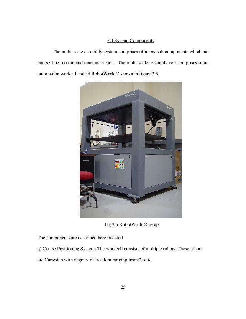


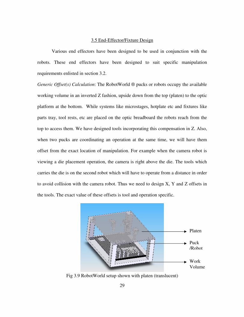

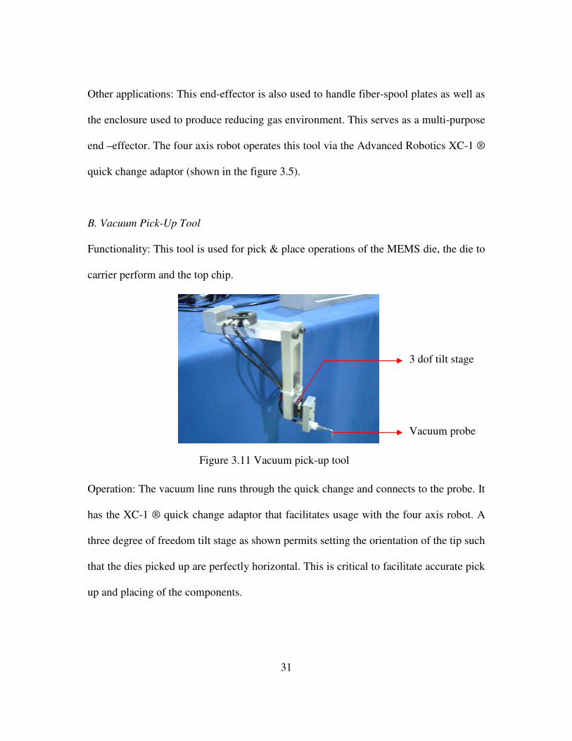


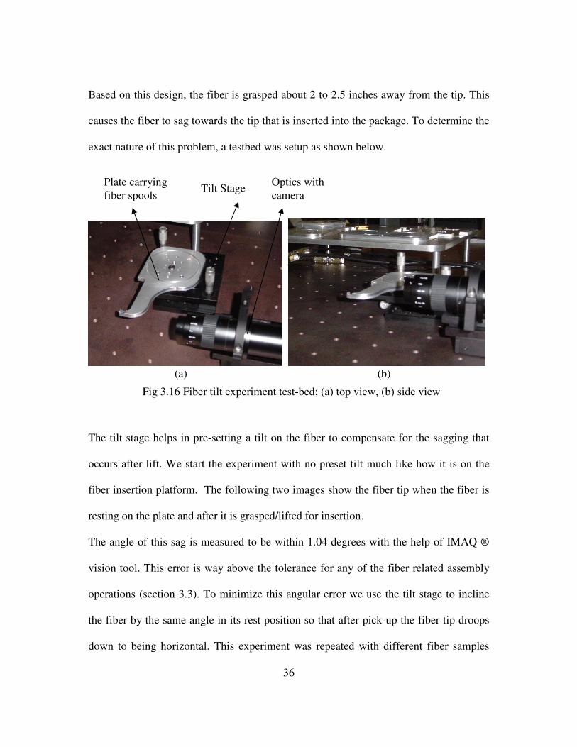


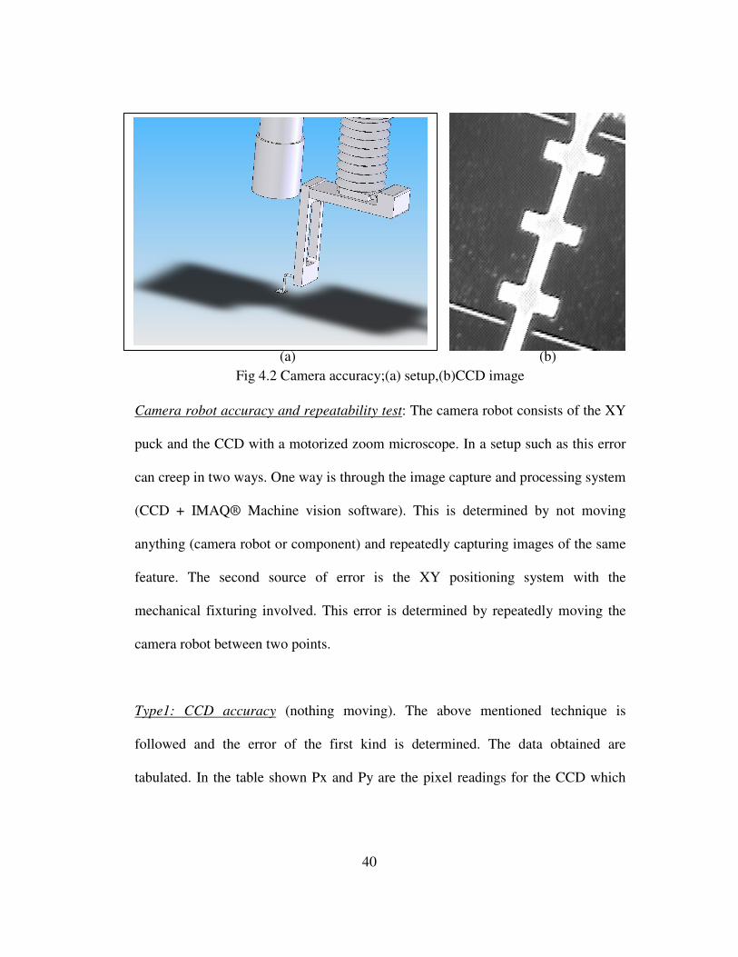


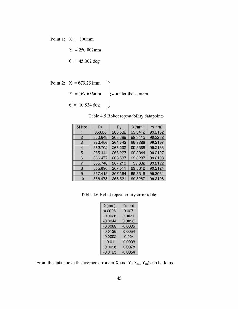


![[L-17] Packaging Schemes for MEMS](https://static.documents.pub/doc/80x56/577d2e641a28ab4e1eaee7ec/l-17-packaging-schemes-for-mems.jpg)


