1

Please note that this is an author-produced PDF of an article accepted for publication following peer review. The definitive publisher-authenticated version is available on the publisher Web site.

Ocean Modelling March 2016, Volume 99, Pages 75-85 http://dx.doi.org/10.1016/j.ocemod.2015.12.005 http://archimer.ifremer.fr/doc/00309/42060/ © 2016 Elsevier Ltd. All rights reserved.

Achimer http://archimer.ifremer.fr

Modulation of wave-current interactions by horizontal mixing and spatial resolution

Bennis A.-C. 1, * , Dumas Franck 2, Blanke Bruno 3

1 Laboratoire de Morphodynamique Continentale et Côtière, UMR 6143, CNRS-UNICAEN-UR, 24 rue des Tilleuls, Caen 14000, France 2 Dyneco/Physed, Ifremer Centre de Bretagne, ZI Pointe du diable, Plouzané 29280, France 3 Laboratoire de Physique des Océans, UMR 6523, CNRS-Ifremer-UBO-IRD, 6 Avenue Le Gorgeu, 29238 Brest cedex 3, France

* Corresponding author : Anne-Claire Bennis, Tel.: +33231565718; fax: +33231565757 ; email address : anne-claire.bennis@unicaen.fr

Abstract : The mechanics of rip currents are complex, involving interactions between waves, currents, water levels and bathymetry that pose particular challenges for numerical modeling. Horizontal turbulent diffusion in a rip system is difficult to measure using dye dilution or surfzone drifters, as shown by the range of published values for the horizontal diffusion coefficient. Here, we studied the effects of horizontal mixing on wave–current interactions by testing several diffusivity estimates in a fully coupled 3D wave–current model run at two different spatial resolutions. Published results using very low diffusion have found that near the shore the wave rays converge towards the rip channel because of refraction by the currents. We showed that this process is modulated by both horizontal mixing and spatial resolution. We found that, without the feedback of currents on waves, the flow is more sensitive to horizontal mixing, with large alterations, especially offshore, and generally lower velocities. These modifications ascribed to mixing are similar to those induced by the feedback mechanism. When a large mixing coefficient is used: (i) the behavior of the rip system is similar for both coupling modes (i.e., with and without the feedback of currents on waves) and for each resolution; and (ii) the evolution of the flow is more stable over time. Lastly, we show that the horizontal mixing strongly decreases the intensity of the 3D rip velocity, but not its vertical shear, which is mainly dependent on the vertical mixing scheme and on the forcing terms.

Highlights

► We continue the 2D work of Weir et al. (2011) with 3D simulations. ► Reference results depend on both horizontal mixing and spatial resolution. ► CEW and horizontal mixing act on the flow in the same way. ► We express wave-current interactions in term of horizontal mixing. ► The vertical shear of the rip velocity is not changed by horizontal mixing and CEW.

Keywords : Coastal ocean modelling, Nearshore processes, Rip currents, Wave-current interactions, Horizontal mixing

1 Introduction28

Rip currents were first investigated by Shepard (1936), and are studied29

for their important influence on nearshore morphodynamics, cross-shore30

exchanges, and the hazard they pose to swimmers (MacMahan et al., 2006).31

From observations made on La Jolla beach in California, Shepard et al.32

(1941) described the rip structure as being composed of three major features:33

the feeder, the neck and the head. Scientific studies began as qualitative34

descriptions based on observations. Since then, theoretical and numerical35

approaches have been developed for rip currents, using observations for36

validation.37

Rip currents are generated by the hydrodynamic instability resulting38

from wave refraction by currents (Leblond and Tang, 1974; Falques et al.,39

1999; Yu, 2006) and the convergence of longshore currents in regions of40

strong alongshore variations in wave conditions (Long and Ozkan-Haller,41

2005). Transient currents forced by finite crest-length wave breaking also42

create a type of rip current (e.g., Johnson and Pattiaratchi, 2006; Spydell43

and Feddersen, 2009; Clark et al., 2012). The feedback mechanism between44

currents and waves has been reported by several authors (e.g., MacMahan et45

al., 2006) as playing an essential role in the development of the rip system.46

The main numerical studies considering the effects of currents on waves47

(hereafter CEW) reported the following behaviors: a) Leblond and Tang48

(1974) observed a modification of the flux of wave energy by the currents,49

with variability along the longshore coordinate; b) Haas et al. (1998) found50

that CEW reduce the offshore extent of rip currents; c) Yu and Slinn (2003)51

showed that rips are compacted with CEW because of the large decrease in52

the wave flux of momentum induced by wave breaking and explained that53

this decrease is due to changes in wave number (wave ray bending); and d)54

Weir et al. (2011) who complemented the last of these studies by calculating55

the change in the wavefield resulting from wave ray bending and from wave56

energy advected by the current (current flux of wave energy). The latter57

authors expressed wave-current interactions in terms of bottom friction.58

Previous studies investigating the effects of current on waves were carried59

out without explicit turbulence modeling and at high resolution, namely 260

and 3 meters in both horizontal directions for Weir et al. (2011) and Yu and61

Slinn (2003), respectively. Because the systematic use of a spatial resolution62

lower than the size of the tiniest vortex is not possible, due to computational63

limitations, the effects of subgrid-scale processes must be parameterized64

in ocean models (e.g., Sagaut et al., 2013). This is particularly the case65

for horizontal diffusive mixing, which can be included in the horizontal66

2

momentum equations in several ways: i) modelers often use a diffusion67

coefficient that is a function of the grid size, but also of the flow and wave68

field characteristics (e.g., Smagorinsky, 1963; Okubo, 1971; Battjes, 1975);69

and ii) the discretization of the advection terms in an Eulerian framework70

with sigma-coordinates and the discretization of the Laplacian operator also71

generate numerical diffusion (Huang and Spaulding, 2002; Zwillinger, 1989).72

Many studies have discussed this numerical diffusion (e.g., Fortunato and73

Baptista, 1994; Huang and Spaulding, 1996, 2002). Huang and Spaulding74

(2002) compared the advection scheme of Mellor and Blumberg (1985) with75

that of Fortunato and Baptista (1994). They found that both schemes76

produce large artificial diffusion, particularly where the bathymetry is steep.77

The most popular ocean models still use different versions of the schemes of78

Mellor and Blumberg (1985) (e.g., POM, ROMS or MARS) and of Fortunato79

and Baptista (1994) (e.g., POLCOMS).80

The diffusion coefficient for nearshore applications is usually measured81

by dye dilution. The literature usually distinguishes between the absolute82

diffusivity, which characterizes the ensemble behavior of a cloud of particles,83

and the relative diffusivity related to the spreading of the cloud around its84

center of mass. Field studies provide many different values for the diffusion85

coefficient: i) Imann et al. (1971) found a cross-shore absolute diffusivity86

(hereafterKax) between 0.1 m2.s−1 and 5.9 m2.s−1 and an alongshore absolute87

diffusivity (hereafter Kay) between 0 m2.s−1 and 0.17 m2.s−1; ii) The long-88

term observations (O(103)s) of Grant et al. (2005) led to Kay between89

40 m2.s−1 and 80 m2.s−1 with larger values for larger waves; and, iii) Clarke90

et al. (2007) noted that the absolute diffusivity was strongly dependent on91

wave conditions and on the presence of rip currents. Their assessment was92

in the range of 10−1 m2.s−1 to 103 m2.s−1.93

Brown et al. (2009) tested another measurement method in order to94

estimate diffusivity with more accuracy. They used thirty surfzone drifters95

at Sand City (Monterey Bay, California) over 7 days between April and May96

2007. The beach is known for its year-round persistent rip channels with97

predominantly near-shore normal incident waves (MacMahan et al., 2005).98

For a given sea state (the significant wave height and the peak wave period99

were about 1.4 m and 11.4 s, respectively), they found Kax = 2.2 m2.s−1 ±100

0.8 m2.s−1 and Kay = 3.8 m2.s−1 ± 1 m2.s−1. The relative diffusivity was101

estimated as being 1.5 m2.s−1 and 6.5 m2.s−1 and between 1.2 m2.s−1 and102

3.6 m2.s−1 in the cross-shore and alongshore directions, respectively.103

In the present work we used a 3D fully-coupled wave-current model104

to study the sensitivity of the rip system to horizontal mixing used to105

parameterize turbulent diffusion. We tested different diffusivity values in106

3

agreement with the scaling of Brown et al. (2009), extended the bidimensional107

(2D) work of Weir et al. (2011) to three-dimensional (3D) simulations and108

applied the vortex force formalism (McWilliams et al., 2004; Ardhuin et al.,109

2008b; Bennis et al., 2011). The main findings of our study are: a) CEW are110

modulated by horizontal mixing, with maximum impact at high resolution ;111

b) Horizontal mixing acts on the flow in a similar way to CEW; c) CEW are112

negligible when using a high mixing coefficient; and, d) the convergence of113

the waves towards the rip channel is modulated by both horizontal mixing114

and spatial resolution.115

The rest of this paper is organised as follows: the method used, including116

the governing equations and details about the simulations, is described in117

section 2; results are presented in section 3, and we summarize our findings118

in section 4.119

2 Methods120

The 3D fully-coupled MARS-WAVEWATCH III model (more details121

in Bennis et al., 2011, 2014) combines the MARS3D hydrodynamic model122

(Lazure and Dumas, 2008) and the WAVEWATCH III wave model (Tolman,123

2009), hereafter WW3. Exchanges of information between the models are124

managed by the PALM coupler (Buis et al., 2008). We can easily investigate125

the feedback of currents on waves by turning off the coupling in test simula-126

tions. All the results presented here were obtained using a non stationary127

coupling procedure. Results obtained for cases with and without feedback128

are referred to hereafter as WEC+CEW and WEC-only, respectively (WEC129

refers to wave effects on currents and, the behaviors ascribed to CEW were130

obtained from the difference between WEC+CEW and WEC-only fields).131

WW3 is a phase-averaged wave model. The wave action density spectrum132

N (N being a function of time, space, wave number and direction) is solved133

as:134

DN

Dt=Q

σ(1)

where Q represents the total source and sink terms, including non-linear135

interactions, bottom friction, wave dissipation and bottom scattering (more136

details in Tolman (2009)) and σ is the intrinsic wave radian frequency.137

High-order conservative numerical schemes are used for spatial discretization.138

A CFL (Courant-Friedrichs-Lewy) condition exists, binding the discretizations139

in time and in space.140

4

MARS3D uses the pressure projection method to solve the 3D, unsteady,141

Navier-Stokes equations under Boussinesq and hydrostatic assumptions. Fini-142

te difference schemes are used for the spatial discretization performed on143

an Arakawa-C grid (Lazure and Dumas, 2008). The model uses an ADI144

(Alternating Direction Implicit) time scheme (Bourchtein and Bourchtein,145

2006), although, the time step of MARS3D is constrained by the CFL146

condition of WW3 in order to avoid too great a time shift between the147

two models.148

Fig. 1 shows the bathymetry for the problem, given the geometry and149

the computational domain. Since we are interested in rip currents, the rip150

channels are near the center of the domain and periodic boundary conditions151

are used at the lateral boundaries. Neumann boundary conditions are152

employed at the surface and bottom, with the additional parameterization153

according to Soulsby (1995) for bottom friction (Bennis et al., 2014). Offshore,154

open boundary conditions are applied based on the method of characteristics155

(e.g., Zwillinger, 1989). This method consists in complementing the physical156

boundary conditions using characteristic pathways around which the solution157

is computed. The scheme of Walstra et al. (2000) is used to parameterize158

the modification of vertical mixing by waves near the surface and bottom.159

The flow is forced by the normal propagation of an incident wave on a160

barred beach. Each test case uses a regular horizontal grid. The time step161

varies according to the size of the mesh to ensure the numerical stability162

of the models and the time synchronization of the coupled system. The163

coupling time step is also different from the time steps of the two models.164

Figure 1: Bathymetry

5

2.1 Governing equations165

Wave forcing was integrated into the hydrodynamic model with the166

vortex force method (McWilliams et al., 2004; Ardhuin et al., 2008b). This167

method has been validated for surf zone cases (e.g., Kumar et al. (2012),168

Moghimi et al. (2012) and Bennis et al. (2014)) and gives good agreement169

with in-situ and laboratory data. The main advantage of the method is170

to consider the mean flow instead of the total momentum (Ardhuin et al.,171

2008b; Bennis et al., 2011), avoiding the difficult modeling of the vertical172

flux of momentum (Ardhuin et al., 2008a).173

The equations of motion for a wave-forced, 3D, incompressible, unsteady,174

hydrostatic, constant-density flow are given in Ardhuin et al. (2008b) and175

Bennis et al. (2011). Their generic formulation is:176

DUDt

= SEPG + SVM + SHM + SWP177

+ SBA + SBBL + SVF (2)178

where U = (U, V,W ) is the 3D quasi-Eulerian velocity computed as the179

Lagrangian velocity minus the Stokes drift. The source terms SEPG, SVM,180

SHM, SBA, SBBL, SVF and SWP refer to the external pressure gradient,181

vertical mixing, horizontal mixing, breaking acceleration, streaming, vortex182

force and wave-induced pressure gradient, respectively. These equations are183

similar those of McWilliams et al. (2004) used in Uchiyama et al. (2010) and184

Kumar et al. (2012).185

The k-ε turbulent closure scheme, modified according to Walstra et al.186

(2000), is used to model vertical mixing (Bennis et al., 2014). Horizontal187

mixing is computed as:188

SHM,x =1

ρ

∂(ρνH

∂U∂x

)∂x

+∂(ρνH

∂U∂y

)∂y

(3)

SHM,y =1

ρ

∂(ρνH

∂V∂x

)∂x

+∂(ρνH

∂V∂y

)∂y

(4)

where SHM,x and SHM,y are the cross-shore and alongshore components189

of SHM, respectively. ρ is the water density, and νH is the turbulent190

kinematic viscosity also known as turbulent diffusivity. Here, νH is constant191

horizontally, with values between 0.2m2.s−1 and 3.9m2.s−1 (see below for192

6

more details). Kumar et al. (2012) also used 0.2m2.s−1 to simulate rip193

currents while Yu and Slinn (2003) used a numerical diffusivity to suppress194

the sub-grid scale noise.195

As the rip system is very sensitive to the modeling of wave breaking, we196

choose the same parameterization for wave breaking dissipation as Weir et197

al. (2011) and Yu and Slinn (2003). The well-referenced parameterizations198

of Thornton and Guza (1983) (hereafter TG83) and Church and Thornton199

(1993) (hereafter CT93) were therefore implemented in WW3 according to200

the following formulations:201

• CT93:202

QCT93 = 1.5√πfpB

3Hrms

hM

1− 1(1 +

(HrmsHm

)2)5/2

F (k, θ), (5)

where M = 1 + tanh

(8

(Hrms

Hm− 1

)). Hrms is the root-mean square203

significant wave height, Hm is the maximum height that can be reached204

by waves without breaking (here Hm = γh, where γ is a tunable model205

parameter and h is the water depth), fp is the peak wave frequency,206

B is a tunable model parameter, k is the mean wave number, θ is the207

mean wave direction, and F (k, θ) is the wave spectrum.208

• TG83:209

QTG83 = 48√πfpB

3 (2m0)5/2

H4mh

F (k, θ), (6)

where m0 is the 0-order moment of the variance density directional210

spectrum. To fit the data, B and γ are set to 1.52 and 0.35, respectively.211

QCT93 or QTG83 are included in the wave action equation computed by212

WW3 (see Eq. (1)) as a fraction, Qbr, of the Q term. Qbr is equal toεbρgσ

213

of Yu and Slinn (2003) and Weir et al. (2011), where εb is their dissipation214

function. To compute SBA in Eq. (2), Qbr is integrated over all directions215

and wave numbers and then distributed over a characteristic depth:216

SBA =

∫(kx, ky)

kCgQbr(k, θ)δzdkdθ (7)

7

where kx = k cos θ, ky = k sin θ and where δz allows the distribution of SBA217

over the water column. Cg is the wave group velocity. SBA is equivalent to218

B in eq. (9) from Weir et al. (2011).219

2.2 Experiments220

We aimed to study the dependence of the flow response on horizontal221

mixing and compared the two coupling modes. In our model, the bedform222

is an approxi-223

mation of the beach profile measured at Duck, North Carolina, on October224

11, 1990 (Fig. 1). Its analytical expression, h(x, y), was given by Yu and225

Slinn (2003) as:226

h0(x) =

(a1 −

a1γ1

)tanh

(b1x

a1

)(8)

+b1x

γ1− a2 exp

[−5

(x− xcxc

)2]

where xc = 80 m is the location of the longshore bar. γ1, a1, b1 and a2227

are set to 11.74, 2.97 m, 0.075, 1.5 m, respectively. Adding a perturbation228

at the longshore bar, the following bottom profile is obtained:229

h(x, y) = h0(x) + h1(x, y) (9)

with230

h1(x, y) = h0(x)ε cos

(2πy

λ

)exp

[−5

(x− xcxc

)2]

(10)

where ε = 0.1 m and λ = 256 m are the magnitude and the wavelength231

of the perturbation, respectively. Weir et al. (2011) used a perturbation232

that was only very slightly different from this one.233

A narrow Gaussian wave spectrum is used at the offshore boundary to234

simulate monochromatic waves as in Weir et al. (2011). The offshore wave235

characteristics and some information on bottom topography are given in236

Table 1.237

The loss of information caused by the use of a coarse grid should be noted238

and need to develop more suitable parameterizations in the future. After239

testing resolutions of 3, 6, 12 and 24 m, we discuss here the results with 3240

and 24-m of spatial resolution because they are the most representative ones241

for the study of the resolution effects.242

8

Parameter Value

Significant wave height Hs = 1.3 mPeak wave period T = 10 sMean wave direction θ = 90◦

Magnitude of perturbation ε = 0.1Spacing of rip channels λ = 256 m

Table 1: Common characteristics of all simulations

Sixteen different test cases were carried out that differed in their horizontal243

resolution, horizontal mixing and coupling mode (Table 2).244

The coupling time step is set to 1 s while the model time step is 0.2 s and245

0.5 s for WW3 and MARS3D, respectively. The simulated time is one hour246

for each simulation. We used 15 sigma levels that are evenly distributed247

over the vertical. Both coupling modes (WEC-only and WEC+CEW) use248

the same set of parameters to ensure a comparison as clean as possible. For249

each resolution, sensitivity tests on mixing were carried out with a variable250

νH (Table 2). The maximum values of νH are in the range given by Brown251

et al. (2009). After many tests, we did not keep the values greater than252

2.0 m2.s−1 (for the resolution of 3 m) and 3.9 m2.s−1 (24 m) because they253

added no new information. Finally, the values of 3.9 m2.s−1 and 0.35 m2.s−1254

were given by Okubo (1971) for resolutions of 24 m and 3 m, respectively.255

νH =0.2 m2/s

νH =0.35 m2/s

νH =0.6 m2/s

νH =1.0 m2/s

νH =2.0 m2/s

νH =3.9 m2/s

∆xy =3 m

WEC-only x x x x xWEC+CEW x x x x x

∆xy =24 m

WEC-only x x xWEC+CEW x x x

Table 2: List of test cases for different spatial resolutions and horizontalmixing intensities.

9

3 Results256

As mentioned in Brown et al. (2009), for a similar wave forcing (Hs =257

1.4 m, Tp = 11.4 s and θ = 0◦), the absolute and relative diffusivites are258

within the ranges[3.1 m2.s−1; 5.6 m2.s−1

]and

[1.9 m2.s−1; 7.4 m2.s−1

], respec-259

tively. We chose νH within these ranges with a maximum set at 3.9 m2.s−1 to260

improve our understanding of the rip system in these realistic hydrodynamic261

conditions. For comparison with the former studies of Yu and Slinn (2003),262

Weir et al. (2011) and Kumar et al. (2012), we also used smaller diffusivities263

down to the stability limit of the model, with a minimum value of 0.2 m2.s−1.264

As the former studies of Yu and Slinn (2003) and of Weir et al. (2011) did265

not use a diffusion coefficient, but an artificial diffusivity not mentioned in266

their papers, we consider that our case with νH = 0.2 m2.s−1 to be almost267

equivalent to their test case. So, we investigated the impact of the value268

of νH on wave-current interactions for two different spatial resolutions (3269

and 24 meters). The high-resolution simulations use mixing coefficients270

between 0.2 m2.s−1 and 2.0 m2.s−1. The coefficients ranged from 0.35 m2.s−1271

to 3.9 m2.s−1 at low resolution.272

The waves come from offshore with a significant wave height of 1.3273

meters and a peak wave period of 10 seconds. Figure 2 shows for both274

parameterizations (TG83 and CT93) the alongshore-averaged root mean275

square significant wave height (< Hrms >) and the alongshore-averaged wave276

breaking dissipation flux (< Φoc >) as a function of the cross-shore distance.277

The wave shoaling is small due to the beach slope and the offshore conditions.278

Wave heights are higher when using the CT93 breaking parameterization,279

which makes the rip unstable as explained in Weir et al (2011). < Φoc >280

shows two peaks, each of which related to a different breaking event. All the281

parameterizations predict that the highest peak is located approximately282

150 meters from the shore. The shapes of < Hrms > and < Φoc > are283

similar to the ones described in Yu and Slinn (2003) and Weir et al. (2011).284

In the following, TG83 is used for all the simulations.285

The total change in Hrms (∆Hrms) ascribed to CEW is shown as a286

function of the cross-shore distance in Figure 3. ∆Hrms is caused by wave ray287

bending, which is dependent on the alongshore gradient of the rip current,288

and also by the current velocity flux (see Weir et al., 2011, for more details).289

At the highest resolution, the two processes interact. From now, the ’shallow290

depths’ term refers to depths less than 2 m located at a distance up to 100 m291

from the shore. Over shallow depths, ∆Hrms is negative showing that the292

effects of the current flux of wave energy are dominant. Elsewhere, we293

observe positive values inside the rip channel and negative values outside it294

10

Figure 2: Alongshore-averaged root-mean square significant wave height(left panel) and alongshore-averaged wave breaking dissipation flux (rightpanel) computed by the TG83 and CT93 parameterizations.

(Figure 3, top row). As a result, the modulation of the wave height by CEW295

is generated by wave ray bending for νH = 0.35 m2.s−1 and νH = 2.0 m2.s−1.296

For the same mixing coefficient (νH = 0.35 m2.s−1), the maximum of ∆Hrms297

is about 0.04 m at high resolution while it reaches about 0.016 m at a spatial298

resolution of 24 m. Near the shore (X ≤ 100 m), wave ray bending slightly299

dominates and two regions with positive values of ∆Hrms appear (Figure 3,300

bottom-left panel). For νH = 3.9 m2.s−1, the increase in wave height inside301

the rip channel becomes negligible (about 0.005 m). Indeed, the horizontal302

diffusivity is too high, leading to a large reduction in the rip velocity and its303

alongshore gradient. Therefore, the interactions with waves are significantly304

affected by mixing.305

Figure 4 shows the alongshore perturbation of the wave group velocity306

computed as the difference between the local wave group velocity and the307

alonghore-averaged value. These snapshots show the simulations run at308

high resolution. These wave fields show that CEW cause wave divergence309

by refraction. For the WEC-only case, we have only refraction by bottom310

topography, which drives the waves towards the peak of the bar (Figure311

4, top plot). When CEW are activated, refraction by currents moves the312

waves towards the rip channel (Figure 4, middle and bottom plots). When313

the smallest mixing coefficient is used (νH = 0.2 m2.s−1), refraction by314

11

Figure 3: ∆Hrms after 60 minutes. Top row: simulations with νH =0.35 m2.s−1 (left panel) and with νH = 2.0 m2.s−1 (right panel) at a spatialresolution of 3m. Bottom row: simulations with νH = 0.35 m2.s−1 (leftpanel) and with νH = 3.9 m2.s−1 (right panel) at a resolution of 24m.Contours are equally spaced between −0.038 m and 0.038 m.

currents dominates refraction by bottom topography near the shore. Thus,315

waves converge towards the rip channel (Figure 4, middle plot). Horizontal316

mixing modifies the interactions between the two refraction processes: the317

higher the mixing coefficient, the weaker the rip velocity and its alongshore318

gradient. As a result, near the shore and with νH = 2.0 m2.s−1, refraction319

by bottom topography dominates refraction by the rip current because the320

alongshore gradient of the rip current is decreased by the mixing. Thus, the321

effects of the rip current are not strong enough to balance the effects of the322

bottom topography. Finally, over shallow depths, the waves diverge from323

the rip channel towards the peak of the bar (Figure 4, bottom plot).324

Figure 5 shows the alongshore component of the wave group velocity325

for νH = 0.35 m2.s−1 and νH = 3.9 m2.s−1. The results are shown for326

both computational grids. As explained above, refraction by bathymetry327

generates divergence towards the bar due to positive values of Cgy to the328

right of the channel and negative values to the left (Figure 5, first column).329

12

Figure 4: Alongshore perturbation of the high-resolution wave group velocity(blue arrows) at t=60 minutes: WEC-only with νH = 0.2 m2.s−1 (top panel),WEC+CEW with νH = 0.2 m2.s−1 (middle panel) and WEC+CEW withνH = 2.0 m2.s−1 (bottom panel). Bathymetry is shown by black dashedcontours.

13

Refraction by currents modifies the direction, and thus produces an inverse330

wave motion leading to negative values of Cgy to the right of the channel and331

positive values to the left (Figure 5, last column). At low resolution with332

νH = 3.9 m2.s−1, wave diversion by the rip current is very weak and CEW are333

not strong enough to overcome the effects of refraction by bathymetry where334

the depth is shallow; therefore, the WEC+CEW alongshore group velocity335

looks like that of the WEC-only case (Figure 5, bottom -left and -middle336

plots). At the same spatial resolution with νH = 0.35 m2.s−1, the patterns337

caused by current refraction are present for the WEC+CEW case. Indeed,338

as the mixing is strongly decreased from 3.9 m2.s−1 to 0.35 m2.s−1, the rip339

velocity and its alongshore gradient are larger and therefore interact with the340

waves. Near the shore (X ≤ 100m), we observe a special situation for which341

the effects of the two refraction processes cancel each other out (Figure 5,342

central plot): waves go straight to the shore. At the highest resolution and343

with the same mixing coefficient (νH = 0.35 m2.s−1), different patterns are344

observed for Cgy, showing the impact of spatial resolution on the wave field.345

Because the bathymetry and rip system are better represented on a finer346

grid, wave-current interactions are simulated more accurately.347

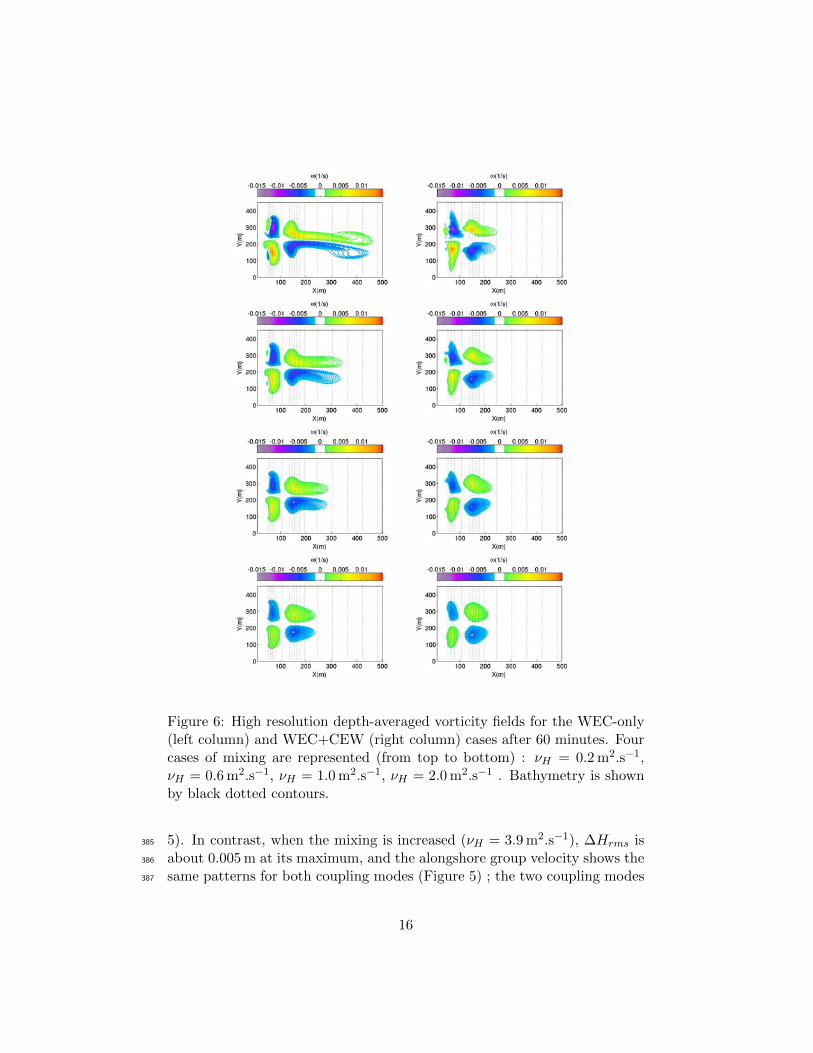
Figure 6 shows the high-resolution depth-averaged vorticity fields for the348

WEC-only and WEC+CEW cases and for different values of νH (0.2 m2.s−1,349

0.6 m2.s−1, 1.0 m2.s−1 and 2.0 m2.s−1). CEW reduce the offshore extension350

of the flow in each case because they produce forcing effects opposed to351

that of the topography (Yu and Slinn, 2003). Horizontal mixing, by its352

smoothing effect on the flow, also contributes to an attenuation of the353

offshore rip system. Therefore, horizontal mixing and CEW act similarly354

on the WEC-only vorticity field, and it is be possible to express CEW in355

terms of horizontal mixing: the WEC-only vorticity computed with νH =356

2.0 m2.s−1 is similar to the WEC+CEW vorticity obtained with νH =357

1.0 m2.s−1 (Figure 6). When νH = 2.0 m2.s−1, the WEC+CEW and WEC-358

only fields look similar because horizontal mixing and CEW move WEC-only359

closer to WEC+CEW. Furthermore, we note that the WEC+CEW flow is360

less altered by horizontal mixing (notably with weaker offshore reduction)361

than the WEC-only flow. Compared with Weir et al. (2011), the evolution362

of the rip system at high resolution is not modified by horizontal mixing for363

νH = 0.35 m2.s−1 (Figure 7). When CEW are activated, the rip system is364

stable after 20 minutes (Figure 7, bottom row), but, the system continues365

to grow offshore for the WEC-only case. Horizontal mixing stabilizes the366

WEC-only flow, and thus modifies its evolution, which becomes similar to367

the WEC+CEW case, when the mixing coefficient is high (Figure 6, bottom368

row).369

14

Figure 5: Cgy for cases WEC-only, WEC+CEW and CEW shown from leftto right. Top row: ∆xy = 3 m and νH = 0.35 m2.s−1. Middle row: ∆xy =24 m and νH = 0.35 m2.s−1. Bottom row: ∆xy = 24 m and νH = 3.9 m2.s−1.All figures are plotted after 60 minutes. Contours are equally spaced from−0.21 m.s−1 to 0.21 m.s−1.

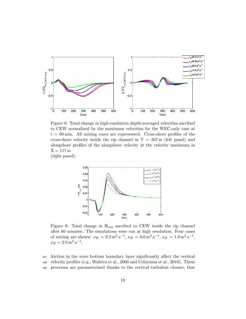
Figure 8 shows the depth-averaged cross-shore and alongshore velocities370

normalized by the maximum velocity of the WEC-only case. Several mixing371

cases and both coupling modes are shown for the simulations run at 3-m372

spatial resolution. We observed that the cross-shore velocity was more373

altered by mixing and CEW than by the alongshore velocity. As waves374

propagate normally to the shore, an alongshore motion is generated by375

refraction. For νH = 0.2 m2.s−1, CEW decrease the cross-shore velocity by a376

factor equivalent to 50% of the maximum WEC-only velocity. The higher the377

mixing coefficient, the more this factor is reduced. For νH = 2.0 m2.s−1, we378

observe a reduction by a factor equivalent to 18%. As the cross-shore velocity379

is modified, interactions with waves are also changed. So, the increase of380

Hrms by CEW is also halved between the 0.2 m2.s−1 and 2.0 m2.s−1 cases381

(Figure 9). A ratio of two is maintained between the rip velocity and the382

wave height. The simulations run at low resolution show that even a small383

∆Hrms (0.015 m at its maximum) modifies the wave fields by CEW (Figure384

15

Figure 6: High resolution depth-averaged vorticity fields for the WEC-only(left column) and WEC+CEW (right column) cases after 60 minutes. Fourcases of mixing are represented (from top to bottom) : νH = 0.2 m2.s−1,νH = 0.6 m2.s−1, νH = 1.0 m2.s−1, νH = 2.0 m2.s−1 . Bathymetry is shownby black dotted contours.

5). In contrast, when the mixing is increased (νH = 3.9 m2.s−1), ∆Hrms is385

about 0.005 m at its maximum, and the alongshore group velocity shows the386

same patterns for both coupling modes (Figure 5) ; the two coupling modes387

16

give similar results.388

Figure 7: Evolution over time of the high-resolution depth-averagedvorticity for νH = 0.35 m2.s−1 : WEC-only (top row) and WEC+CEW(bottom row). Colored contours are equally spaced between −0.015 s−1 and0.015 s−1. Bathymetry is shown by black dotted contours.

Figure 10 shows the vertical profiles of the high-resolution 3D cross-shore389

velocity inside the rip channel. As in Kumar et al. (2012), the maximum rip390

velocity is located within the water column, and the rip current decreases391

towards the bottom and the surface. The vertical profiles are changed392

by CEW. The WEC-only velocity is more intense than the WEC+CEW393

velocity, particularly when the mixing coefficient is weak. For a diffusion394

coefficient of 0.2 m2.s−1, CEW reduce the maximum cross-shore velocity395

by 25%, whereas we obtain a 8% reduction with a diffusion coefficient of396

2.0 m2.s−1. As for the barotropic fields, the offshore extension of the rip397

system is reduced by CEW and horizontal mixing. Mixing causes maximum398

alterations for the WEC-only case for which the maximum 3D velocity is399

reduced by 20% between the 0.2 m2.s−1 and 2.0 m2.s−1 cases whereas this400

reduction is limited to 3% when CEW are activated.401

Horizontal mixing does not modify the vertical shear of the rip velocity402

because it modifies each 2D slice of the horizontal velocity equally in the403

vertical. This shows that the vertical structure is mainly forced by the404

set of equations used to compute the wave-current interactions, and also405

by the vertical mixing scheme. Wave breaking and dissipation by bottom406

17

Figure 8: Total change in high-resolution depth-averaged velocities ascribedto CEW normalized by the maximum velocities for the WEC-only case att = 60 min. All mixing cases are represented. Cross-shore profiles of thecross-shore velocity inside the rip channel in Y = 267 m (left panel) andalongshore profiles of the alongshore velocity at the velocity maximum inX = 117 m(right panel).

Figure 9: Total change in Hrms ascribed to CEW inside the rip channelafter 60 minutes. The simulations were run at high resolution. Four casesof mixing are shown: νH = 0.2 m2.s−1, νH = 0.6 m2.s−1, νH = 1.0 m2.s−1,νH = 2.0 m2.s−1.

friction in the wave bottom boundary layer significantly affect the vertical407

velocity profiles (e.g., Walstra et al., 2000 and Uchiyama et al., 2010). These408

processes are parameterized thanks to the vertical turbulent closure, that409

18

was modified to this end. The mathematical modelling of the wave-current410

interactions also influences the vertical profiles, as discussed in Ardhuin411

et al. (2008b) and Bennis et al. (2011). CEW appear too weak to change412

the vertical shear and act similarly to the horizontal mixing by reducing the413

intensity of the rip current and its offshore extension. Lastly, as reported by414

some previous authors (e.g., Kumar et al., 2012; Teles, 2013), the structure of415

the rip velocity varies with depth. Thus, 3D simulations are useful because416

the vertical profiles cannot be deduced from 2D runs. These profiles are417

very important when studying hydro-sedimentary motions inside the water418

column but also near the bottom.419

Figure 10: High resolution cross-shore profiles of the 3D cross-shore velocitytaken inside the rip channel for the WEC-only (top row) and WEC+CEW(bottom row) cases after 60 minutes. Four cases of mixing are representedwith from left to right: νH = 0.2 m2.s−1, νH = 0.6 m2.s−1, νH = 1.0 m2.s−1,νH = 2.0 m2.s−1. Colored contours are equally-spaced between −0.5 m.s−1

and 0.5 m.s−1.

4 Summary and conclusions420

Field measurement of diffusivity in rip current systems is difficult and421

many different values exist in the literature. In this paper, we numerically422

tested different ranges of diffusivity values in order to improve our understan-423

ding of the sensitivity of the rip system to this kind of mixing. Our test case424

was the same as that used by Weir et al. (2011) and Yu and Slinn (2003), and425

we started by revisiting their experiments. As explained above, we consider426

that we can reproduce their results by using the smallest diffusion coefficient427

(0.2 m2.s−1); a section of this paper concerns the validation of our approach.428

19

We then tested different diffusivity values in the range of the observations429

of Brown et al. (2009) for a similar wave forcing, with a maximum value of430

3.9 m2.s−1 given by Okubo (1971). For all cases, the simulations are 3D,431

in contrast with the previous 2D studies that were performed with spatial432

resolutions of 3-m and 2-m. This allows us to highlight the importance433

of 3D effects. Two different spatial resolutions (3 m and 24 m) were also434

tested for different diffusivity values in order to understand the link between435

mixing, spatial resolution and wave-current interactions. For each case, we436

investigated how the hydrodynamic conditions and spatial resolution change437

the wave-current interactions in a 3D framework.438

Our 2D results, obtained by integrating the horizontal momentum over439

depth, for a diffusion coefficient set at 0.2 m2.s−1 and with a 3-m spatial440

resolution, were tested against the results of Weir et al. (2011) and Yu441

and Slinn (2003). Our simulations showed a rip system quite similar to442

these previous studies: i) refraction by currents dominates refraction by443

bathymetry for shallow depths, which induces a wave motion towards the444

rip channel; ii) changes in wave height and wave number are produced by445

CEW; iii) CEW significantly reduce the offshore flow because they produce446

an opposite forcing to the rip motion, and thus block the system’s growth,447

iv) CEW decrease the intensity of the flow; and, v) the flow is stabilized448

by CEW. This validation shows that our 3D model is able to correctly449

reproduce the 2D flow simulated by pure 2D models. We conclude that the450

3D effects have little impact on the depth-averaged flow although the flow451

shows vertical shear. This could be because the vertical shear is not strong452

enough to significantly impact the barotropic fields, noting that the set of453

equations of Bennis et al. (2011) is valid only for a weak shear. When the454

shear is stronger, and in these cases with the inclusion of the shear-induced455

pressure term of Ardhuin et al. (2008b) given in their eq. (40), the 3D effects456

could significantly modify the depth-averaged flow.457

The horizontal resolution modifies wave-current interactions because of458

the coarse description of the bathymetry. For the same value of mixing459

coefficient (0.35 m2.s−1), the change in wave height is reduced by a factor of460

two when the calculations are run at low resolution. This change is generated461

by nearshore wave ray bending and by the current velocity flux, as shown462

in Weir et al. (2011). At low resolution, waves go straight to the beach463

because wave diversion by bathymetry exactly compensates wave divergence464

by currents. This result suggests that the refraction by bathymetry needs465

to be parameterized in coarse resolution models.466

When we use a mixing coefficient above 0.2 m2.s−1, the waves go to the467

peak of the bar instead of converging on the rip channel. This shows that468

20

refraction by bathymetry is dominant, and thus mixing changes the balance469

between the two refraction processes. For a diffusivity of 2.0 m2.s−1, the470

high-resolution depth-averaged vorticity without CEW is similar to the one471

obtained with CEW, because they have a weaker impact on the flow. We472

observed the same behavior at low resolution for νH = 3.9 m2.s−1. We noted473

that the high-resolution vorticity field computed without feedback and with474

νH = 2.0 m2.s−1 looks like the one obtained for the WEC+CEW case with475

νH = 1.0 m2.s−1. We noted that mixing and CEW act in the same way:476

horizontal mixing reduces the offshore extension of the system, smooths477

the rip velocities and their alongshore gradients and stabilizes the flow.478

Thus, it modifies the interactions with the waves. The maximum alterations479

ascribed to mixing are found for the WEC-only case, showing that this480

flow is more sensitive than the WEC+CEW flow. At high resolution, the481

maximum value of the 3D cross-shore velocity is reduced by 20% between482

the 0.2 m2.s−1 and 2.0 m2.s−1 cases, whereas this reduction is limited to 3%483

when CEW are activated. For the largest values of the diffusivity (2 m2.s−1484

and 3.9 m2.s−1), the WEC-only and WEC+CEW flow patterns are similar.485

We hypothesize that mixing processes suppress the part of the flow that486

would be in disagreement with the WEC+CEW flow, indicating that the487

WEC-only solution for a diffusivity less than 2 m2.s−1 might not be realistic.488

For all cases, the vertical shear of the 3D cross-shore velocity is not489

modified by CEW or horizontal mixing, which shows that it is strongly490

dependent on the vertical mixing scheme and on the forcing terms. In491

contrast, the intensity of the 3D velocity is strongly affected both by CEW492

and horizontal mixing, with similar effects. For a diffusion coefficient of493

0.2 m2.s−1, CEW reduce the maximum 3D cross-shore velocity by 25%,494

whereas we obtain an 8% reduction with a diffusion coefficient of 2.0 m2.s−1.495

The two mechanisms decrease the velocity and its alongshore gradient, and496

reduce its offshore extension.497

To conclude, horizontal mixing was found to have direct impacts on498

wave-current interactions. We showed that the conclusions of Weir et al.499

(2011) and Yu and Slinn (2003) depend on both horizontal mixing and500

spatial resolution. When a larger mixing is used (here above 2.5 m2.s−1),501

CEW vanish. This result is important because the wave-current models502

are also used to simulate coastal seas where mixing is taken into account503

to represent subgrid scale processes. In the future, these results could be504

applied to 3D morphodynamic studies.505

21

5 Acknowledgments506

The authors thank B. Weir for his expert advice and F. Ardhuin for his help507

and the useful comments. The authors thank three anonymous reviewers508

for their input. A.-C. B. is supported by the Universite de Caen Normandie.509

A.-C. B. also acknowledges the support of a post-doctoral grant from Universi-510

te de Bretagne Occidentale, and the PREVIMER project. A.-C. B. was also511

supported by a FP7-ERC grant number 240009 for the IOWAGA project.512

F.D. is supported by Ifremer and the PREVIMER project. B.B. is supported513

by CNRS.514

References515

Ardhuin, F., A. D. Jenkins, and K. Belibassakis, 2008a: Commentary on ‘the516

three-dimensional current and surface wave equations’ by George Mellor.517

J. Phys. Oceanogr., 38, 1340–1349.518

Ardhuin, F., N. Rascle, and K. A. Belibassakis, 2008b: Explicit519

wave-averaged primitive equations using a generalized Lagrangian mean.520

Ocean Modelling, 20, 35–60, doi:10.1016/j.ocemod.2007.07.001.521

Battjes, J. A., 1975: Modelling of turbulence in surf zone. Symposium on522

Modelling Techniques, San Francisco, ASCE, 1050–1061.523

Bennis, A.-C., F. Ardhuin, and F. Dumas, 2011: On the coupling of524

wave and three-dimensional circulation models: Choice of theoretical525

framework, practical implementation and adiabatic tests. Ocean526

Modelling, 40, 260–272.527

Bennis, A.-C., F. Dumas, F. Ardhuin, and B. Blanke, 2014: Mixing528

parameterization: impacts on rip currents and wave set-up. Ocean529

Engineering, 42, 213–227.530

Bourchtein, A. and L. Bourchtein, 2006: Modified time splitting scheme for531

shallow water equations. Mathematics and Computers in Simulation, 73,532

52–64.533

Brown, J., J. MacMahan, A. Reiners, and E. Thornton, 2009: Surf zone534

diffusivity on a rip-channeled beach. J. Geophys. Res., 114, C11 015.535

Buis, S., A. Piacentini, and D. Declat, 2008: PALM: A computational536

framework for assembling high performance computing applications.537

Concurrency Computat.: Pract. Exper., 18 (2), 247–262.538

22

Church, J. C. and E. B. Thornton, 1993: Effects of breaking wave induced539

turbulence within a longshore current model. Coastal Eng., 20, 1–28.540

Clark, D. B., S. Elgar, and B. Raubenheimer, 2012: Vorticity generation by541

short-crested wave breaking. Geophys. Res. Lett., 39, L24 604.542

Clarke, L., D. Ackerman, and J. Largier, 2007: Dye dispersion in the543

surfzone: Measurements and simple models. Continental Shelf Research,544

27, 650–669.545

Falques, A., A. Montoto, and D. Vila, 1999: A note on hydrodynamic546

instabilities and horizontal circulation in the surf zone. J. Geophys. Res.,547

104 (C9), 20 605–20 615.548

Fortunato, A. and A. Baptista, 1994: Localized sigma coordinates for549

the vertical structure of hydrodynamic models. Proceedings of the Third550

International Conference on Estuarine and Coastal Modeling, New York.551

Grant, S., J. H. Kim, B. H. Jones, S. A. Jenkins, and J. Wasyl, 2005: Surf552

zone entrainment along-shore transport and human health implications of553

pollution from tidal outlets. J. Geophys. Res., 110, C10 025.554

Haas, K. A., I. A. Svendsen, and M. C. Haller, 1998: Numerical modeling555

of nearshore circulations on a barred beach with rip channels, paper556

presented at the 26th conference on coastal engineering. Am. Soc. of Civ.557

Eng.558

Huang, W. and M. Spaulding, 1996: Modelling horizontal diffusion with559

sigma coordinate system. Journal of Hydraulic Engineering, 122, 349–352.560

Huang, W. and M. Spaulding, 2002: Reducing horizontal diffusion561

errors in σ-coordinate coastal ocean models with a second-order562

lagrangian-interpolation finite-difference scheme. Ocean Engineering, 29,563

495–512.564

Imann, D. L., R. J. Trait, and C. E. Nordstrom, 1971: Mixing in the565

surfzone. J. Geophys. Res., 76, 3493–3514.566

Johnson, D. and C. Pattiaratchi, 2006: Boussinesq modelling of transient567

rip currents. Coastal Engineering, 53, 419–439.568

Kumar, N., G. Voulgaris, J. C. Warner, and M. Olabarrieta,569

2012: Implementation of the vortex force formalism in the coupled570

ocean-atmosphere-wave-sediment transport (COAWST) modeling system571

for inner shelf and surf zone applications. Ocean Modelling, 47, 65–95.572

23

Lazure, P. and F. Dumas, 2008: An external-internal mode coupling for a573

3d hydrodynamical model for applications at regional scale (MARS). Adv.574

Water Resources, 31, 233–250.575

Leblond, P. H. and C. L. Tang, 1974: On energy coupling between waves576

and rip currents. J. Geophys. Res., 79, 811–816.577

Long, J. W. and H. T. Ozkan-Haller, 2005: Offshore controls on nearshore578

rip currents. J. Geophys. Res., 110, C12 007, doi:10.1029/2005JC003018.579

MacMahan, J. H., E. B. Thornton, and A. J. Reniers, 2006: Rip current580

review. Coastal Eng., 53, 191–208.581

MacMahan, J. H., E. B. Thornton, T. P. Stanton, and A. J. H. M. Reniers,582

2005: RIPEX-Rip currents on a shore-connected shoal beach. Marine583

Geology, 218, 113–134.584

McWilliams, J. C., J. M. Restrepo, and E. M. Lane, 2004: An asymptotic585

theory for the interaction of waves and currents in coastal waters. J. Fluid586

Mech., 511, 135–178.587

Mellor, G. L. and A. F. Blumberg, 1985: Modelling vertical and horizontal588

diffusivities with the sigma coordinate system. Monthly Weather Review,589

113, 1379–1383.590

Moghimi, S., K. Klingbeil, U. Grawe, and H. Burchard, 2012: A direct591

comparison of the depth-dependent radiation stress method and a592

vortex force formulation within a three-dimensional ocean model. Ocean593

Modelling, 1–38.594

Okubo, A., 1971: Oceanic diffusion diagram. Deep Sea Research, 18,595

789–802.596

Sagaut, P., S. Deck, and M. Terracol, 2013: Multiscale and multiresolution597

approaches in turbulence, 2nd edition. Imperial College Press, 450 pp.598

Shepard, F. P., 1936: Undertow, rip tide or rip current. Science, 84, 181–182.599

Shepard, F. P., K. O. Emery, and E. C. L. Fond, 1941: Rip currents: A600

process of geological importance. Journal of Geology, 49, 337–369.601

Smagorinsky, J., 1963: General circulations experiments with the primitive602

equations i. the basic experiment. Monthly Weather Review, 8, 99–165.603

24

Soulsby, R. L., 1995: Bed shear stresses due to combined waves and604

currents. In: Stive, M., Fredsøe, J., Hamm, L., Soulsby, R., Teisson,605

C., Winterwerp, J. (Eds). Advances in Coastal Morphodynamics, Delft606

Hydraulics, Delft, The Netherlands, 420–423.607

Spydell, M. and F. Feddersen, 2009: Lagrangian drifter dispersion in the surf608

zone: Directionally spread, normally incident waves. J. Phys. Oceanogr.,609

39, 809–830.610

Teles, M. J., 2013: Wave-current modelling at local and regional scales.611

Ph.D. thesis, Instituto Superior Tecnico, Lisbon, Portugal.612

Thornton, E. B. and R. T. Guza, 1983: Transformation of wave height613

distribution. J. Geophys. Res., 88 (C10), 5,925–5,938.614

Tolman, H. L., 2009: User manual and system documentation615

of WAVEWATCH-IIITM version 3.14. Tech. Rep. 276,616

NOAA/NWS/NCEP/MMAB.617

Uchiyama, Y., J. C. McWilliams, and A. F. Shchepetkin, 2010:618

Wave-current interaction in oceanic circulation model with a vortex-force619

formalism Application to the surf zone. Ocean Modelling, 34, 16–35.620

Walstra, D. J. R., J. Roelvink, and J. Groeneweg, 2000: Calculation of621

wave-driven currents in a 3D mean flow model. Proceedings of the 27th622

international conference on coastal engineering, Sydney, ASCE, Vol. 2,623

1050–1063.624

Weir, B., Y. Uchiyama, E. M. Lane, J. M. Restrepo, and J. C. McWilliams,625

2011: A vortex force analysis of the interaction of rip currents and surface626

gravity waves. J. Geophys. Res., 116, C05 001.627

Yu, J., 2006: On the instability leading to rip currents due to wave-current628

interaction. J. Fluid Mech., 549, 403–428.629

Yu, J. and D. N. Slinn, 2003: Effects of wave-current interaction on rip630

currents. J. Geophys. Res., 108 (C3), 3088.631

Zwillinger, D., 1989: Handbook of differential equations. Academic Press,632

1-665 pp.633

25