MODULATIONAL STABILITY OF OSCILLATORY PULSE SOLUTIONS OF THE PARAMETRICALLY-FORCED NONLINEAR SCHRODINGER EQUATION Paul Augustine Chin-Yik Chang B.Sc. Simon Fraser University, 1999 M.Sc. Simon Fraser University, 200 1 A THESIS SUBMITTED IN PARTIAL FULFILLMENT OF THE REQUIREMENTS FOR THE DEGREE OF DOCTOR OF PHILOSOPHY IN THE DEPARTMENT OF MATHEMATICS O Paul Chang 2003 SIMON FRASER UNIVERSITY December, 2003 All rights reserved. This work may not be reproduced in whole or in part, by photocopy or other means, without permission of the author.
Transcript
MODULATIONAL STABILITY OF OSCILLATORY PULSE SOLUTIONS OF THE PARAMETRICALLY-FORCED
NONLINEAR SCHRODINGER EQUATION
Paul Augustine Chin-Yik Chang B.Sc. Simon Fraser University, 1999 M.Sc. Simon Fraser University, 200 1
A THESIS SUBMITTED IN PARTIAL FULFILLMENT OF THE REQUIREMENTS FOR THE DEGREE OF
DOCTOR OF PHILOSOPHY
IN THE DEPARTMENT OF MATHEMATICS
O Paul Chang 2003 SIMON FRASER UNIVERSITY
December, 2003
All rights reserved. This work may not be reproduced in whole or in part, by photocopy
or other means, without permission of the author.
APPROVAL
Name: Degree: Title of Thesis:
Examining Committee:
Paul Chang Doctor of Philosophy Modulational Stability of Oscillatory Pulse Solutions of the Parametrically~Forced Nonlinear Schrodinger Equation Dr. S t e p h n Chair Assistant r f ss r
I
~ r x x h goMslow Senior Supervisor Associate Professor
-
Associate Professor
Dr. Ralf ~ i t tenbefg Supervisor Assistwt Professor
- ~- Dr. Brian Wetton Internal External Examiner Associate Professor Mathematics Department Univmity of British Columbia
Dr. Robert L. Pego External Examiner Professor Department of Mathematics University of Maryland
Date Approved: December 8, 2003
PARTIAL COPYRIGHT LICENCE
I hereby grant to Simon Fraser University the right to lend my thesis, project or
extended essay (the title of which is shown below) to users of the Simon Fraser
University Library, and to make partial or single copies only for such users or in
response to a request from the library of any other university, or other educational
institution, on its own behalf or for one of its users. I further agree that permission for
multiple copying of this work for scholarly purposes may be granted by me or the
Dean of Graduate Studies. It is understood that copying or publication of this work
for financial gain shall not be allowed without my written permission.
Title of Thesis/Project/Extended Essay
Modulational Stability of Oscillatory Pulse Solutions of the Parametrically-Forced Nonlinear Schriidinger Equation
Author: - (signature)
(name)
(date)
ABSTRACT
We employ a global quasi-stationary manifold to rigorously reduce the parametrically
forced nonlinear Schrodinger equation (PNLS) to a finite-dimensional flow. While this man-
ifold is not invariant, the long-time evolution of the full system is captured as a flow on the
manifold through a renormalization group method. An explicit ODE for the flow is derived.
Using this ODE, we show that the stationary pulse solution of the PNLS undergoes a Hopf
bifurcation in a certain parameter regime, and that there exists a stable oscillatory limit cycle
beyond criticality. In particular, we show that the Hopf bifurcation is supercritical.
DEDICATION
I dedicate this tome to Kiki for motivating me to work hard.
ACKNOWLEDGMENTS
I would like to thank Keith for his tremendous patience and guidance. I would also
like to thank Ralf for his helpful comments and meticulous attention to detail. And I would
like to thank all my committee members for reading thls thesis.
TABLE OF CONTENTS
APPROVAL ........................................................................... ii
We study the parametrically forced nonlinear Schrodinger equation (PNLS):
where y and a are the forcing and detuning parameters respectively. With this scaling, the
dissipationless case corresponds to a --t co. This equation describes a wide variety of physical
phenomena, including the optical parametric oscillator in the large pumpdetuning limit,
Faraday resonance in water, spin waves and magnetic solitons in ferromagnets, and phase-
sensitive parametric amplification of solitons in optical fibres [2, 5, 111. For sufficiently strong
parametric excitation, y > I , the system can produce and sustain the solitonic waves
where
The lower branch solution 4- exists only when y E , and it is always unstable due
to the presence of point spectrum in the right-half complex plane [3]. We therefore disregard
4- and study only the local behaviour and stability properties of the upper branch solution
4+. Direct computer simulations were previously done in the stable [3] and unstable [5] regions
in the parameter plane which revealed that the existence of two internal oscillation modes
of 4+. For a > a2 z 2.645, the system undergoes a Hopf bifurcation as y increase. beyond
the critical value y, (a) , and these modes resonate to produce a stable oscillatory solution for
1
y E (y, (a) , d m ) . This is accompanied by a complex conjugate pair of eigenvalues of the
associated linearized operator crossing the imaginary axis into the right-half complex plane
161.
Previous work was done in [2] in which the supercritical dynamics of d+ were described
analytically. The oscillatory solution was expressed as a perturbation expansion about @+,
and reduced amplitude equations governing the nonlinear evolutions were obtained. The goals
of this thesis are to extend this body of work as follows. First, we analyze the stability and
long-time behaviour of the oscillatory solution itself. In doing so, we also obtain an analytic
description of the behaviour of nearby solutions. The conditions under which these descrip
tions are valid are also investigated. Lastly, we explicitly show that the Hopf bifurcation is
supercritical. Our results are summarized in Theorem 19. We note, however, that our inves-
tigations are valid for the fully dissipative case only (finite a ) , whereas the authors in [2] also
investigated the stability problem for the dissipationless case (a -+ m). In the latter case,
the mechanism of soliton instability is due to the oscillatory-instability bifurcation, which is
characterized by the collision of two pure imaginary eigenvalues of the associated linearized
operator, one detaching from the essential spectrum and the other originating from the broken
U (1) gauge invariance [3].
The PNLS also possesss the trivial solution 4 = 0. It is stable when the forcing
parameter is small, y E 0, d m , and unstable against essential spectrum perturbations ( ) when the forcing parameter is large, y E (&+a2, m ) . As with 4-, we also disregard this
solution.
In [6], the Hopf bifurcation curve y = y, (a) was computed by constructing Dirichlet
expansions on the stable manifold of the eigenvalue problem associated with the linearization
of the PNLS about @+. This expansion was then used to construct the Evans function, a
Bifurcation Diagram
Figure 1.1: Bifurcation Diagram for the PNLS.
Wronskian-like analytic function whose zeros coincide with the eigenvalues of the linearized
operator. The Evans function is particularly useful for detecting bifurcations because the
order of the zero is equal to the algebraic multiplicity of the eigenvalue [I]. The technique
used in [6] was also used in [13] to analyze the polarizational mode instability in birefringent
fiber optics. Using the Evans function for the PNLS, the following stability diagram was
obtained.
As y increases from 1, the Hopf eigenvalues travel in the complex plane as follows [6].
To describe the eigenvalue trajectories which accompany the Hopf bifurcation, it is convenient
to rescale the eigenvalue X of the linearized operator as J = X /v+: The scaled eigenvalues
enjoy four-fold symmetry with respect to the point -1 in the sense that, if J is a scaled
eigenvalue, then so are z, -2 - J, and -2 - J. The linearized operator possesses the scaled
eigenvalues J = 0, -2 and the scaled essential spectrum
ce,waled ( L ) = { ~ = x + i y l x E (-1 - J=!-I+ J-)! y = O
or x = -1, y E (-m, -Jq] LJ (J-,m)}. (1.5)
Consider f i s t the case a > a1 = 1.132. As y increases from 1, the scaled eigenvalue JH
leaves the origin along the real axis towards -1, while the scaled eigenvalue tE bifurcates out
from the essential spectrum through the point - 1 + id= along the line - 1 + iy towards
- 1. Although the scaled essential spectrum also expands along - 1 + iy towards - 1, its edge
always trails behind JE. AS y further increases, J H collides with its symmetrical counterpart
-2 - JH at -1. It then makes a right angle turn and moves along -1 + iy towards JE. JH
then collides with JE at some critical value of y before moving off towards the imaginary axis.
tH and its symmetrical counterpart then cross the imaginary axis as y increases through
y, (a), and the Hopf bifurcation results.
Meanwhile, as y increases, the scaled essential spectrum forms a "cross" centered at
-1, and it eventually crosses the origin along the real axis. An essential bifurcation then
results. For a E (al , ag), the essential bifurcation occurs before the Hopf bifurcation, so @+
remains stable for its domain of existence. For a E (ag, m ) , the Hopf bifurcation occurs first,
at which point 4, becomes unstable and an oscillatory wave solution emerges.
The case a < a1 is similar to that of a > a1 except that the eigenvalues bifurcate off
of the real axis rather than along the line -1 + iy.
In the next chapter, we illustrate our methods by applying them to a toy example. We
then proceed in the subsequent chapter to analyze the PNLS.
Essential Spectrum
T 'N
Essential Spectrum 'N
J Hopf Eigenvalue
J Zero Eigenvalue
J Hopf Eigenvalue
K y=2.4
-10 L -3 -2.5 -2 -1.5 -1 -0.5 0 05 1
Figure 1.2: Scaled eigenvalue trajectory for increasing y and fixed a = 2.8.
CHAPTER 2.
THE TOY EXAMPLE SYSTEM
The problems and solutions presented in this chapter is a simplified version of the ideas
presented in [17]. In the next chapter wherein we will analyze the PNLS, those methods will
be a slight generalization.
The purpose of this chapter is to illustrate the methods we will use to analyze the
PNLS. We do so by applying these methods to an ODE problem. Our goal is to determine
the long-time behaviour and stability properties of a quasi-stationary solution of an ODE
We do so by constructing a (not necessarily invariant) manifold parametrized by q which
contains the quasi-stationary solutions Qq which we study. We then reduce the flow onto M ̂
through the decomposition
where W is the residual term. Our problem thus becomes one of identifying the flow on
the manifold and obtaining estimates on W. The decay estimates which characterize these
manifolds are exponential in nature, and are often obtained from the semigroup generated by
the linearization Lq = F' (Qq).
We describe the flow on the manifold using a series of local coordinate systems tied
to the manifold itself. These coordinate systems are not chosen a priori however, but rather
are selected to adapt to the flow on the manifold as the flow evolves. A key condition which
characterizes our problem is that Z evolves slowly along the direction of the manifold. This
enables us to control and remove the secularity through a slow modulation of the parameters
and renormalization.
6
To explain our problem more precisely, let us discuss the properties of the linearization
which characterize our problem. We then present the toy example and give an overview of
our activities in this chapter. Our main results are summarized in Theorem 5.
2.1 Description of the ODE Problem
Let
Z , = F ( Z ) , K I P - l R n , Z € R n
be an ODE which possesses an attractive manifold M ̂of stationary solutions Q, parametrized
by q E RE, fi < n:
M - 1 1 Q, P (Q , )=o , P E R ' , f i < n j . (2.4)
Suppose we perturb this ODE by shifting a bifurcation parameter or adding small terms to
F: say, thereby transforming (2.3) to
A
In particular, this perturbation is such that M becomes a quasi-stationary manifold with
respect to (2.5) in the sense that
llF (Qq) ll = 0 ( 6 ) (2.6)
for some small parameter 6. What then remains of G ? What are the new dynamics near
G ?
To further characterize our problem, let us expand solutions of (2.5) as
( 4 = Q,(t) + W ( t ) , (2.7)
where Qq is the quasi-stationary solution which shadows Z on M ̂and W is a small residual
term. Substituting this decomposition into (2.5) and linearizing F about Qq yields
where
is the n by fi matrix containing the partial derivatives of Qq with respect to the components
of q,
is the linearization of F about Qq, and
contains the higher-order nonlinear terms in ..
Figure 2.1 : Schematic picture of the decomposition (2.7).
The following conditions characterize our problem.
Condition 1 (Normal Hyperbolicity) The spectmm of each operator Lq may be decom-
posed into a stable part a; strictly contained in the left-half complex plane and an active part
aq comprised of a jixed number of eigenvalues with small real part. In particular,
where a, is contained in { z E @ IRer 5 -k ) for some k > 0 and oq, which consists of
ezgenvalues including multiplicity, is contained in { z E @ I IRe zl 5 6) for some positive 6 < k .
Both k and % do not depend on q.
perturbation X - Figure 2.2: Schematic picture of the spectrum of the perturbed and unperturbed linearized
operator, ODE case.
The fi-dimensional Lq-invariant subspace associated with aq is denoted by Xq and
is called the active space. It contains the salient dynamics of the ODE. The complementary
subspace of dimension n - % is denoted X i and is called the stable space. Under the action
of Lq, members of X< satisfy the following decay estimate.
Condition 2 (Semigroup) Each operator Lq generates a semigroup Sq which satisfies
for some constant c~ >_ 1, for all Z E Xi, and for all t 2 0. The constant c~ is chosen to be
independent of q.
9
The semigroup decay estimate (2.13) is uniform in q in the sense that the constant
cs does not depend on q, but this estimate is only applicable for each fixed q. We wish to
exploit this estimate to bound the residual term W but the corresponding manifold parameter
function q = q (t) varies with time t . Fortunately, q is seen to evolve slowly for the class of
problems which we consider, so given the initial condition
at the initial time tb, Lb will approximate L, well for a long time after tb. We are thus
motivated to impose the condition
W E X b (2.15)
under which W will decay under the action of Lb in accordance with (2.13). Bounds on W
can then be obtained by exploiting (2.13). These bounds will be obtained for the toy example
of this chapter in Sections 2.4 and 2.5. Observe that (2.15) implies that both W,t and Lb W
also lie in X i .
The price for imposing the condition (2.15) is the appearance of a secular term which
grows as q evolves away from b. To see this, we "anchor" all q-dependent terms in (2.8) to
b like
A, = Ab + (Aq - Ab) ,
where 4 represents any q-dependent term, which recasts (2.8) as
Tbq,t + W,t = F (Qb) + LbW + Nb (W) + Sb (q, W) :
where
Sb (qI W) - ( F (Q,) + LqW + Nq (W) - f ,q,t)
- ( F ( Q ~ ) + LbW f Nb ( W ) - 4bq.t)
10
is the secular term. All terms in (2.17) except for Sb depend on b and not on q while Sb
is at most 0 (lq - bl). Since q evolves slowly, Sb is guaranteed to be small compared to the
other quantities in (2.17) for a long time after tb. In essence, then, Sb may be ignored until
it grows to a size comparable to the other quantities in (2.17). This eventual happenstance
and its resolution is addressed for the toy example of this chapter in Section 2.5.
The time t b and the point b are hereby called the anchor time and anchor point
respectively.
A
The eigenvectors of Lq which span Xq are denoted by Q$) , j = 1, ..., N, and the
corresponding adjoint eigenvectors by Q$It. The corresponding eigenvalues are denoted by
A j . The spectral projection operators corresponding to Xq and Xi are denoted by xq and
x; respectively.
The evolution equation for q is obtained as follows. Taking the inner product of each
side of (2.17) with Q t ) t yields
where we have used the fact that WYt, LbW E X i , and where we have introduced the matrix
The following condition guarantees the solvability of (2.19) for q,t.
Condition 3 (Compatibility) The matrix fiq is uniformly boundedly invertible i n q. In
particular, we require the manifold parameters and eigenvectors to be ordered i n such a way
that
fi, = I + 0 ( E ) ,
where I is the identity matrix and E is a small parameter.
Provided that this condition is satisfied, we may multiply both sides of (2.19) by fib1
to obtain the equation
s,t = W b (W) + Z b ((4, W) (2.22)
which determines the evolution of q, where
The evolution equation for W is obtained by projecting (2.17) onto Xi
Substituting q,t (2.22), we rewrite (2.25) as
where
Lastly, we substitute q,, (2.22) into Sb (2.18) to obtain
which implicitly defines Sb.
2.2 The Tov Exam~le Svstem
We now illustrate our methods by applying them to a toy example.
12
Notation The following notation is employed throughout this chapter only. Transposition
is denoted by the superscript t. The components of a vector quantity A are denoted by
A = (al , ~ 2 ) ~ . The inner product (. 1 . ) of two real vectors A and B is defined as
This inner product induces the norm 1 1 . 1 1 which in turn induces the operator norm II.II+. The
adjoint of an operator L with respect to (. 1. ) is denoted by L+. The differentiation operator
with respect to the variable x is denoted by d,, and its action on a function f is denoted
by d, f = f,,. Quantities will be enumerated with the superscript ( j ) , where j = 0,1 ,2 , . . ..
Constants are denoted by cteXt, where "text" is an abbreviated description of the constant.
Description of the TES The unperturbed ODE which we study in this section is
where f E c2 (B, B), and it and its derivatives are uniformly bounded:
for some constant cf. Examples off include f (I) = sin i, f (n) = sech I, or f ( r ) = (1 + n2)
for instance. (2.31) possesses the manifold
of stationary solutions Q, which coincides with the curve z2 = f ( q ) in the qz2-plane.
h h
Solutions of (2.31) near M are driven onto M along trajectories parallel to the i2-axis.
We perturb (2.31) by adding the following terms. In the following, it is assumed that
6 is a sufficiently small positive constant such that
6cf < c d < 1 (2.34)
13
[ ~ n ~ e r t u r b e d Sys tem
Figure 2.3: Solution of the unperturbed ODE.
for some positive constant cd. Imagining that Z represents the position of a virtual particle,
the term (6, o ) ~ represents "wind" which pushes the virtual particle along 22 = f (zl), while
(-bf' ( q ) , o ) ~ represents "gravity1' which tends to push the particle forward if it is on a
( t
downslope, and backwards if on an upslope. The nonlinear term (f ( a ) - 0) takes
into account that the "wind" is stronger the further the particle is away from 22 = f (zl).
Adding these terms to (2.31) yields the perturbed ODE which we call the Toy Example
System (TES):
h
With respect to (2.35), M is now a quasi-stationary manifold in the sense that /IF (Q,)II =
0 (6).
Our goal is to analyze the long-time evolution of TES solutions and their stability
properties. We also wish to obtain the initial conditions and class of TES problems (i.e.
bounds on b) under which our analysis holds. To describe the evolution of solutions Z near
Perturbed System
W Z 1
Figure 2.4: Solution of the perturbed ODE.
2, we decompose Z as
and substitute into the flow F (2.35) and linearize about the quasi-stationary solution Qq
(2.33). We then anchor q to an anchor point b, and the secularity in the system becomes
apparent via the appearance of the term Sb ( q , W ) (2.18). By projecting the resulting evolution
equation onto the active space Xb and the stable space X;, the evolution equations for q and
W are obtained. We then solve for the mild solution (2.74) for W from which we obtain the
decay estimate (2.123) for W valid for the current anchor point b. This estimate shows that
control of Mi is lost after a finite time period, and this is caused by secular growth. We then
remove this secularity by rechoosing our anchor point to b* in such a way that W E XG.
This is done by Theorem 4. Lastly, we show that by appropriately choosing the &xed time
length At in which each anchor point is used (see 2.144), the TES solution will approach and
remain near the manifold under suitable initial conditions.
15
Imd
T perturbation - d
;1; = tif 'l(q) b Red
Figure 2.5: Spectrum of the un [perturbed and perturbed linearized operator.
The Linearized Operator Ln this section, we calculate the linearized operator Lq, its adjoint
L;, and their eigenvalues and eigenvectors. Lq possesses a small eigenvalue Xq = -6 f" (q) and
a fired eigenvalue A; = - 1, and its stable space X; is spanned by a fked vector yl; = (0, I ) ~ .
While these properties are nongeneric in the sense that @; does not depend on q, it does not
diminish the generality of our methods. Lastly, we determine the semigroup decay estimate
(2.50) which will be used to bound the residual term W.
For economy of notation, denote
Under the assumptions (2.32,2.34), nq is 0 (1) and its denominator is uniformly bounded
away from zero.
The linearized operator
possesses the eigenvalue-eigenvector pair
associated with the active space X,. It also possesses the eigenvalue-eigenvect or pair
associated with the stable space Xq-. Some remarks are in order. First, X; does not depend
on q since both AQ and \Ir; do not. Second, Xq- is infinite-dimensional for the PDE case,
so no PDE analogues of X i and Q; exist. Lastly, the expressions (2.39,2.41) for X q and XQ
show that the Normal Hyperbolicity condition is satisfied.
The adjoint linearized operator
possesses the eigenvectors
which correspond to the eigenvalues A, and A; respectively. Both adjoint eigenvectors have
been normalized so that ( A ] A + ) = 1, where A = Qq, Q;
17
The operator which spectrally projects onto the active space X, is given by
Its complementary operator which spectrally projects onto the stable space X; is given by
where I is the identity operator.
The relation (L,Z 2 ) = - 112112 holds for all Z E X;. The restriction of L, to X i
therefore generates a strongly continuous semigroup of contractions Sq which satisfies the
estimate
for all Z E X; and t 1 0. This shows that the Semigroup condition is satisfied with both cs
and k equal to 1.
2.3 The Evolution Eauations
In this section, we compute explicit expressions for the evolution equations (2.22,2.26)
for q and W. This primarily involves computing explicit expressions for wb (W) (2.23) and
S Z b ( W ) (2 .27) . We then obtain the mild solution (2.74) for W .
For the TES, wb (W) (2.23) is given by
The terms comprising wb ( W ) are computed as follows. First, fjq is obtained by differentiating
Qq (2.33):
and then taking the inner product with P i (2.44):
The Compatibility condition is thus satisfied. Next, direct substitution of the solution Q,
(2.33) into the flow F (2.35) and subsequent dotting with Q; (2.44) yields
Finally, since Qb_ = (0, l ) t (2.42) spans X; and since W E X;, we may write W = wPb_ =
(0, w ) ~ where w = 11 Wll. Therefore, it follows by direct calculation that
With these expressions in hand,
wb ( W ) = b (1 - f' (b)) + w2.
Also, for the TES, Zb (q, W) (2.24) is given b y
The evolution equation (2.22) for q is thus explicitly given by
For the TES, Clb ( W ) (2.27) is given by
Using the operator ;rb (2.49) to spectrally project F (Qb) , Nb ( W ) , and Y b onto X; yields
With these expressions in hand,
0 s ( W ) = 6 (M!') + 6Mj2)) + w2 (Mj3) + 6Mb(l)) , (2.67)
where
. .
are 0 (1) quantities which depend only on b. Also, for the TES, Sb (q, W) (2.24) is given by
- s b ( 9 , W ) = ~ ; ( ~ b ( 9 ~ w ) - f b ( ~ b ( 9 , ~ ) ~ ~ ~ ) ) . . (2.72)
The evolution equation (2.26) for W is thus explicitly given by
where ab (W) and Sb (q, W) are given as above, and it possesses the mild solution
w (t) = S (t - tb) Wb + S (t - T) Gb (T) d ~ ,
where the "forcing term" Gb is given by
and Wb E W (tb) is the initial residual with respect to the anchor point b.
2.4 Bounds on the Residual Term
From the mild solution (2.74) for W, we obtain the estimate (2.123) for W valid for
the current anchor point b. This estimate shows that control of W is lost after a finite time
period, and this is caused by the secular growth in Sb (2.72). We remove this secularity in
the following section by rechoosing our anchor point as b* in such a way that W E X;. This
is done by Theorem 4. Lastly, we show that by appropriately choosing the fixed time length
At in which each anchor point is used (see 2.144), the TES solution will approach and remain
near the manifold under suitable initial conditions.
Introduction Fix the anchor point at b on the time interval Itb, td) and denote the final value
of q on [tb, td] by d. Also denote w - IIWII, and the initial and final values of w on [tb, td] by
wb and wd. The following equations then hold:
The following control quantities play prominent roles in our analysis. The quantity
is the total length of time in which the anchor point b has been in use. The quantity
controls the distance between the manifold position parameter q and the anchor point b, and
the quantity
controls the size of W. W will decay exponentially in accordance with the semigroup decay
estimate (2.50), so the purpose of the exponential factor ee-tb in (2.79) is to compensate for
this decay.
Apply the triangle inequality and the semigroup decay estimate (2.50) to the mild
solution (2.74) for W to obtain
where gb = IIGbll. A bound on Gb is obtained in the next section, which will then be used to
bound W.
Bound on the Forcing Term The goal in this section is to obtain a bound on the "forcing
term" Gb (2.75).
A bound on fib (W) is obtained as follows. By the assumptions (2.32,2.34), nb (2.37)
satisfies
. -
In conjunction with (2.32), we thus see that MP) (2.68 thru 2.71) are uniformly bounded in
b:
where
and where each of the arguments in the definition of CM are bounds on Mf), j = 1 thru 4,
respectively. Applying these estimates for M:) to Rb (W) (2.67) then yields
Bounds on qIt and Sb (q, W) are obtained as follows. Applying the triangle inequality
to (2.18) yields
Let us estimate each of the terms appearing in the right-hand side. Direct substitution of F
(2.35) and ?, (2.53) yields
Thus, by applying the Mean Value Theorem on f' and subsequently the uniform boundedness
assumption (2.32) on f",
Next, since V!; = (0 , l ) ' (2.42) spans Xb and since W E X;, we may write W = wQ; =
(0, w ) ~ . By direct calculation then, LqW = (0, - w ) ~ and N, (W) = (w2, o)', and so
Applying the above estimates to Sb (2.85) and q,t (2.62) then yields
which we combine as
Control of Sb and q,t by the estimates (2.94,2.95) is lost when T(Q) grows too large.
We therefore impose the constraint
which restricts the possible size of At, thereby bounding Sb and qYt as
where c,, max {2cj (2 + cj) , 2cj, 2 (i + cf) ,2). We further impose the condition
which restricts the initial size of the residual to obtain
~ ( 9 ) by its definition (2.78) then satisfies the estimate,
Lastly, a bound on S b (q , W ) is obtained as follows. Applying the triangle inequality
to (2.72) yields
l l g b (q, ~ 1 1 1 5 \lri l\* ( I IS~ (q, W ) \ l + llTbll l ( ~ b (4 , w, IQ!)~) . (2.105)
By direct computation, both nb (2.49) and T b (2.53) have norms less than 1 + c2, and so 6 /Isb ( ( , ~ 1 1 5 c 3 6 2 ~ t , (2.106)
where CJ - JG ( 1 + J-) cis ( I + 2)'. With the bounds (2.84,2.106) for Qb ( W ) and Sb (q, W) in hand, the "forcing term" Gb
(2.75) satisfies the bound
where c, = max { c M + 6cM, c3}.
So long as the constraints ~ ( q ) 5 2 (2.96) and w < c6& (2.99) hold, then the 2cf
estimates (q,tl < cq, (1 + c:) 6 (2.101) and ~ ( 9 ) 5 c,, (1 + c:) 6 A t (2.103) also hold. On the
other hand, if the estimate (2.103) holds, then the constraint (2.96) also holds if
1 c,, ( 1 + c i ) 6 A t 5 -. (2.108)
2cf
It is thus self consistent to replace the constraint (2.96) with the constraint (2.108), and we
do so. Lastly, we rewrite (2.108) as
A t 5 ct6-I,
25
where ct - (2ctcqs ( 1 + c i ) ) -'.
Residual Decay Estimates We assume that the constraints (2.99,2.109) hold, and we apply
the bound (2.107) for Gb to the estimate (2.80) for W to obtain
t ( t ) 5 e-(t-tb)b)Wb + Cy 1 e-(t-7) (w2 (7) + 6 (1 + 6At)) d r , (2.110)
t b
Replacing t with 19, multiplying by eePtb, and taking the supremum over 0 E [tb,td), (2.110)
becomes
T ( ~ ) 5 wb + c, sup ee-tb e-(e-r) (w2 ( 7 ) + 6 ( 1 + d ~ t ) ) d ~ , @ E [ t b , t d )
Since
and
(2.112) may be rewritten as
where
yl ( t ) = 1 - e-t,
y2 ( t ) (et - 1 ) ( 1 + 6t ) .
26
. .
Kote that y2 is a strictly increasing function. The inequality (2.117) implies that either
T(W) < zl or T(") > z2, where zl < zz are the two roots of the quadratic equation
c,yl ( A t ) z2 - + (wb + h b 9 2 ( A t ) ) = 0 . (2.120)
This quadratic equation possesses real solutions so long as its discriminant is positive, and this
is always true for tub and by2 ( A t ) sufficiently small. Since T(") is continuous, T(") (At = 0 ) =
wb, and z2 (At = O f ) = m, it follows that initially T(") ( A t = 0 ) < zl ( A t = 0 ) and hence, by
continuity of T("), q, and z2 with respect to At, the inequality T(") 5 zl holds for all At.
That is, with zl obtained via the quadratic formula, the inequality
holds. By the approximation % 1 - $x then,
where c,, is a constant slightly greater than 1. By further substituting T(") (2.79) and the
inequality yl (At) 5 1, we obtain the residual decay estimate
Moreover, by replacing A t with t - t b and substituting y2 (2.1 lg), we obtain the residual
decay estimate for general time t :
2.5 The Reanchor Method
The evolution equations (2.62,2.73) for q and W remain valid so long as the secular
term Sb (2.18) remains sufficiently small. When this is no longer true, we rechoose the anchor
point to remove this secular growth. Moreover, this new anchor point 6' is chosen so that
the new residual lies in XG. Theorem 4 will show that such a choice exists and is unique,
provided that q is sufficiently close to the old anchor point b and provided that W is sufficiently
small. The price of reanchoring is jump discontinuities in both q and W wherein W could
in principle increase, yet we will show that the residual decay estimate (2.123) controls this
possible growth provided that A t , the length of time in which each anchor point is used, is
suitably long. The residual decay estimate (2.123) is the key estimate whch allows us to
determine such a A t so that secular growth is controlled and removed. Lastly, we will show
that after an initial transient stage wherein the residual decays, the residual will remain small
for all time and so our solution remains close to the manifold for all time.
/ M I Reanchor ~ e t h o d ]
Figure 2.6: The reanchor method, ODE Case.
The Reanchor Method Again, fix the anchor point at b on the time interval [ tb , t d ) and denote
the final value of q on [ta, td] by d- When reanchoring, Z may be decomposed as either
Z = Qd + Wd with respect to the old anchor point b, where Wd E XT, or as Z = Qb- + Wb' with respect to the new anchor point b*, where b* is to be determined so that Wb. E Xb;.
Reanchoring introduces a jump discontinuity in both q and W wherein q jumps from d to b*
. -
and W jumps from Wd to Wb*. Equating these two decompositions and solving for Wb., we
obtain
Wp = Wd + Q d - Qb*. (2.126)
Since Wb. E XG, then
Given d and Wd, the following theorem shows that there exists a unique b* such that (2.127)
is satisfied. In addition, this theorem gives an estimate on the jump discontinuity in q when
reanchoring.
Theorem 4 Express Wd = wdSb for some scnlar wd 2 0 and vector S b E Xr satisfying
llZbll = 1. For wd suficiently small, there exists a unique smooth function 31 : R+ -, R such
that, by choosing b* = d + 31 ( w d ) , (2.127) i s satisfied. M O T ~ O V ~ T , the estimate
holds for some constant G.
Proof. The equation (2.127) is equivalent to I' = 0, where
I' (wd, b*) - wdib + Qd - Qb* / 8:. ) . (
As -Q, , It = -1 and (z, I 8 ; ) = 0 , the partial derivatives of I' are ( I , )
. .
r has a root at ( w d , b*) = (0, d ) and r,b* ( 0 , d ) = -1 which is 0 ( 1 ) ; so the implicit function
theorem guarantees the existence of a smooth function % such that b* = d+% ( w d ) . Moreover,
since r,,, ( 0 , d ) is 0 ( d - b ) , the implicit function theorem implies that I'H' (0)I is 0 ( d - b)
also. The estimate (2.128) then follows from the Mean Value Theorem.
The reanchor method for the TES was presented in greater generality than was needed
for pedagogical reasons. In particular, the unique choice of b* is actually d because X; is
bindependent.
Estimates on the Reanchor Jump Discontinuities Apply the triangle inequality and substitute
Qq (2.33) to the identity (2.126) to obtain
Application of the Mean Value Theorem on f and the uniform boundedness assumption (2.32)
on f' then yields
Inserting the estimate (2.128) for Id - b* 1 and subsequently (2.103) for Id - bl , we then obtain
where CJ E c, 1 + c2c . ( 1 + 4). This estimate shows that w could in principle increase G q
when reanchoring, yet we will show in the next section that the residual decay estimate
(2.123) controls this possible growth provided that At, the length of time in which each
anchor point is used, is suitably long.
30
. .
The Iterations We now investigate two states in which, for some m to be determined, either
wb E (m6, cg&) or wb E 10, m6] respectively. These states are called the initial transient and
asymptotic states. We will show that w decreases on the whole in the initial transient state
in the sense that wb* < wb, while w remains small in the asymptotic state. Moreover, we will
show that we can take At = In (1 + 2 ~ ) and m = y2 (At).
Inserting the residual decay estimate (2.123) into the reanchor jump estimate (2.138)
This inequality holds so long as the two constraints wb < c6& (2.99) and At 5 ct6-' (2.109)
holds. To continue using (2.139), we must rechoose our anchor point before either of these
constraints fail.
Initial Transient State In the initial transient state wherein wb E
impose the constraint
by2 (At) I wb (2.140)
on At and apply it to (2.139) to obtain
where
h (x) = c, (1 + L) (1 + 6 c ~ x ) e-=
We now choose the fixed length of time At in which the current anchor point b is used such
that h (At) z i. (The choice of $ is somewhat arbitrary. As long as h (At) < 1, our analysis
can proceed forward.) By demanding that 6 and cg are sufficiently small such that
the choice
yields
and (2.141) thus becomes
2 Wb* 5 hmwb 5 -Wb.
3
We further choose
so that the constraint (2.140) is automatically satisfied by virtue of the fact that wb E
(m6, c a d ) . It remains to show that our choice of At also satisfies the constraint (2.109),
but this is easily achieved if we demand that 6 satisfy
We have thus proven that, if wb E m6, c a d and At = In (1 + 2&), the residual ( 1 decays on the whole in the sense that wb. < h,wb. Moreover, we have determined the
appropriate initial conditions and the class of TES problems under which our analysis holds.
In particular, the solution must be close enough to the manifold such that the residual satisfies
w (0) < c a d (2.99) where ca is determined by (2.143). Also, the class of TES problems which
we consider are constrained to satisfy (2.149).
The residual will continue to decay until wb E [0, m6] at which point the system enters
the asymptotic state.
32
Asymptotic State In the asymptotic state wherein wb E [0, m b ] , we choose At as in (2.144):
At = In ( 1 + 2 h ) . (2.150)
Since y:, (At) = m and wb < m6, (2.139) then becomes
Wb- < h (4 ( m 6 ) ,
where h is given by (2.142) as before. Since h ( A t ) = h , 5 $, we have
wb- < m6. (2.152)
We have thus proven that, if wb E [0, mb] and At = In ( 1 + 2%), then wb- E [0, mb]
also. In conjunction with the decay estimate (2.123), this shows that
for all time t in the asymptotic state.
2.6 Conclusion
We conclude this chapter with the following theorem which summarizes our results.
Theorem 5 Consider the Toy Example System ( T E S )
where 6 > 0 and f and its derivatives are uniformly bounded. For 6 suficiently small and
w < c&, the T E S posesses the solution
for each jixed anchor point b, where q satisfies the evolution equation ( in the asymptotic state)
and W satisfies the condition
and the bound
w ( t ) I ce-(t-tb) (wb + by2 ( t - t b ) )
with y2 ( t ) ZE (et - 1) (1 + 6t) . Moreover, one can use each anchor point for an 0 ( 1 ) time
period and rechoose the anchor point thereafter according to Theorem 4 such that, i n the initial
transient state, wb. < hmwb for some fixed constant h, < 1 and, i n the asymptotic state,
w I m b for some 0 ( 1 ) constant m.
CHAPTER 3.
THE PNLS
We now generalize the methods from the previous chapter to analyze the PNLS. Our
goal remains to analyze the stability and long-time behaviour of the oscillatory solution itself.
In doing so, we also obtain an analytic description of the behaviour of nearby solutions. The
conditions under which these descriptions are valid are also investigated. Lastly, we explicitly
show that the Hopf bifurcation is supercritical. Our results are summarized in Theorem 19.
We construct a manifold consisting of the upper branch solutions 4+ and the eigen-
functions corresponding to the Hopf eigenvalues of the linearization. The manifold parameters
are
P = (PO,P~,PZ) = (q , r l , r2) , (3.1)
where q describes the position and 11-1 describes the oscillation amplitude. The angular fie-
quency can be obtained from the evolution equation for T. We reduce the flow onto the
manifold and linearize the PNLS about 4+ to obtain a general evolution equation. The
evolution of p and W are then determined by projecting the general evolution equation onto
active space Xb (which corresponds to the zero and Hopf eigenvalues) and the complementary
space Xb (which corresponds to essential spectrum strictly contained in the left-half complex
plane).
As before, we describe the flow on the manifold using a series of local coordinate
systems tied to the manifold itself. These coordinate systems are not chosen a priori however,
but rather are selected to adapt to the flow on the manifold as the flow evolves. Our key
modification of this method from [I?] is that, not only do we adapt the local coordinate
systems, but we also adapt the manifold itself to the flow. In some sense, we are adapting
the manifold to capture higher order modes which also resonate via the Hopf bifurcation (or
. .
perhaps some other mechanism) - higher order modes that are not-adequately captureable
by the unmodified manifold. We speculate that this adaptation also provides a method of
constructing an invariant manifold for the PNLS, but we shall not show this. Only once we
adapt the manifold to the flow are we able to exhibit and classify the Hopf bifurcation.
To explain our problem more precisely, let us discuss the properties of the linearization
which characterize our problem. We then reintroduce the PNLS and give an overview of our
activities in this chapter. We note that the notation for the PDE case is consistent with that
for the ODE case.
3.1 Description of the PDE Problem
Let
2 , = F (2)
be a PDE which possesses an attractive manifold of stationary solutions. Denote this manifold
by M^, the stationary solutions by Qql and the parameters which parametrize this manifold
by q E RR:
G c { ~ q l F ( ~ q ) = ~ , q ~ ~ R } . (3.3)
Suppose we perturb this PDE by, say, shifting a bifurcation parameter or adding small terms
to F, thereby transforming (3.2) to
Z,t = F (2) . (3.4)
In particular, we consider those perturbations which induce bifurcations in the system, thereby
A
inducing new dynarnical behaviour not adequately captureable as a reduced flow on M. To
capture this new behaviour then, we enlarge M^ as
M 5 {a, = Q~ + R~ 1 1 1 F (a,) 1 1 = o (a ) , p = (q, r) E B~ x cN-$} , (3.5)
where b is some small parameter. The N parameters p which parametrize M consist of the
slowly-evolving parameters q and the small complex parameters r.
[phase Space Dajectory
Figure 3.1: Schematic picture of the trajectory p = p (t) in phase space.
To further characterize our problem, let us expand solutions of (3.4) as
where ap is the quasi-stationary solution which shadows Z on M and W is a small residual
term. Substituting this decomposition into (3.4) yields
where
'p -- (dP1aP,dP2ap>"' 7dPNaP) (3.8)
is the vector of partial derivatives of ap with respect to the components of p. Because the
Normal Hyperbolicity and Semigroup conditions pertain to the linearization of F about Q,,
37
we linearize F about Qq (as opposed to Qp) to obtain
where
Lq = F' (Qq)
is the linearization of F about Q, and
contains the higher-order nonlinear terms in ..
Figure 3.2: Schematic picture of the decomposition (3.6).
The following conditions characterize our problem.
Condition 6 (Normal Hyperbolicity) The spectrum of each operator Lq may be decom-
posed into a stable part a; strictly contained in the left-half complex plane and an active part
a, comprised of a @ed number of eigenvalues with small real part. I n particular,
a (L,) = a, U o,,
where a; is contained in {t E @ IRez 5 -k ) for some k > 0 and aq, which consists of N
38
eigenvalues including multiplicity, is contained i n { z E C ] /Re zl 5 6 ) for some positive 6 < k .
Both k and N do not depend on q.
In contrast with the ODE case, o, consists of N eigenvalues rather than fi eigenvalues.
Condition 7 (Semigroup) Each operator Lq generates a Co semzgroup Sq which satisfies
for some constant c~ 2 1, for all Z E X;, and for all t >_ 0. The constant cs is chosen to be
independent of q .
The semigroup decay estimate (3.13) is uniform in q in the sense that the constant
cs does not depend on q, but this estimate is only applicable for each f ied q. We wish to
exploit this estimate to bound the residual term W but the corresponding manifold parameter
function q = q ( t ) varies with time t . Fortunately, though, q is seen to evolve slowly for the
class of problems which we consider. So, given the initial condition
at the initial time tb, Lb will approximate Lq well for a long time after tb. We are thus
motivated to impose the condition
W E X i (3.15)
under which W will decay under the action of Lb in accordance with (3.13). Bounds on W
can then be obtained by exploiting (3.13). These bounds will be obtained for the PNLS in
Sections 3.5 and 3.6. Observe that (3.15) implies that both W,t and LbW also lie in X i .
We stress that only the slowly-evolving parameters q are anchored; the small complex
parameters r are not.
The price for imposing the condition (3.15) is the appearance of a secular term which
grows as q evolves away from b. To see this, we "anchor" all q-dependent terms in (3.9) to
b like
where A, and Ap = represent any q and p dependent term respectively, which recasts
(3.9) as
where
is the secular term. All terms in (3.18) except for Sb depend on b and not on q while Sb
is at most 0 (Iq - b/). Since q evolves slowly, Sb is guaranteed to be small compared to the
other quantities in (3.18) for a long time after tb . In essence, then, Sb may be ignored until
it grows to a size comparable to the other quantities in (3.18). This eventual happenstance
and its resolution is addressed for the PNLS in Section 3.6.
The evolution equation for q is obtained as follows. Taking the inner product of each
side of (3.18) with Q ? ) ~ , we then obtain
where
The following condition guarantees the solvability of (3.26) for p,t.
Condition 8 (Compatibility) T h e matr ix II, is uniformly boundedly invertible in p. In
particular, we require the manifold parameters and eigenfunctions t o be ordered in such a way
that
where I is the identi ty matria: and E i s a small parameter.
It will be shown that E = Irl for the PNLS. Provided that this condition is satisfied,
we may multiply both sides of (3.20) by II&) to obtain the equation
which determines the evolution of p, where
The evolution equation for W is obtained by projecting (3.18) onto Xb:
Substituting the equation (3.23) for p,t, we rewrite (3.26) as
which determines the evolution of W, where
Lastly, we may substitute the equation (3.23) for p,t into Sb (3.19) to obtain
which implicitly defines Sb.
To have M capture the dynamics of nearby solutions well, we require that W decays
until it remains small. For instance, we require that W decay to 0 ( r 4 ) for the PNLS so that
the reduced flow on M and its associated ODE can demonstrate the Hopf bifurcation and the
existence of a stable oscillatory limit cycle beyond criticality. Because W is the same order
as Sib ( r , W) in the asymptotic state, this requirement is equivalent to the following condition
on Qb (r, W ) .
Condition 9 (Quasi-Invariant Manifold) For each anchor point b, the modified mani-
fold must be chosen so that
n b ( r , 0 ) = 0 (0 (3.31)
for some small parameter 5. and all time t .
3.2 The PNLS
Notation The following notation is employed throughout this chapter only. Transposition
is denoted by the superscript t . The components of a vector quantity A are denoted by
A = (al , The L~ inner product (. 1 . ) of two complex vectors A and B is defined as
This inner product induces the L~ norm ) ( . 11 and Hs norm ( 1 . / I H S which in turn induce the
operator norms /I . ( 1 , and 1 1 . ( ( * , J S respectively. The orthogonal complement in L~ is denoted
by I. Given an operator A, its adjoint with respect to (- 1.) is denoted by A+, and its spectrum
and resolvent sets by a (A) and p ( A ) . Quantities associated with a complex variable z include
its complex conjugate Z, its magnitude It./ and argument argz, and its real and imaginary
parts Re z and Im t. The differentiation operator with respect to the variable x is denoted
by a,, and its action on a function f is denoted by a, f = f,,. Quantities will be enumerated
with the superscript (j), where j = 0,1,2, . . .. Constants are denoted by ctext, where "text"
is an abbreviated description of the constant. Lastly, we will use the (slightly bad) notation
Description of the PNLS Denote
We rescale the dependent and independent variables of the PNLS (1.1) as
and drop the tilde notation to recast (1.1) as
Introducing
Z = (zl , z2)t = (Re 9,1m $)t
with 121 = , /z lz + 2 2 8 , we vectorize (3.35) to obtain the vectorized PNLS
where
and
p = v+/v-.
For a E (0, m) and y E (1, ~m), the PNLS possesses the manifold
of stationary pulse solutions Q,, where
s, (x) = h s e c h (x - q) .
Note that s, is simply the solitary wave solution q5+ with the scalings (3.34) applied.
As discussed in the introduction, the PNLS undergoes a Hopf bifurcation as y is
increased beyond y, (a) for fixed a > a, = 2.645. To show this and to capture the resulting
oscillatory pulse solution, we must enlarge M ̂ by adding new parameters and new terms.
But how should this be done? Because the PNLS possesses two simple Hopf eigenvalues at
criticality, let us add two small parameters 7-1 and 7-2:
Note that the index in p starts at 0, not 1. We then expand the correction term Rp in powers
of 7-1 and 7-2 as
The Stationary Pulse Solution
Figure 3.3: The stationary pulse solution of the PNLS.
Figure 3.4: Conceptual picture of the solution of the PNLS.
45
where
and RP) , Rkk), and Rfk') are 0 (1) terms. Higher order correction terms need not be
considered, as will be shown later. We now select Rf) so that the Compatibility condition
is satisfied, while we select Rfk) and Rfkl) so that the Quasi-Invariant Manifold condition is
satisfied.
We satisfy the Compatibility condition as follows. The modified manifold M consists
with tangent plane spanned by
where we have introduced the symmetry condition Rfk) = RY) . To satisfy the Compatibility
condition aPkQp d j ) ' = djk +O ( E ) , where djk are the components of the Kronecker delta, ( I q ) we choose
where Qfv) are the eigenfunctions of the linearized operator L, corresponding to the Hopf
(0) eigenvalues Xj, j = 1,2. (It will later be shown that Q,,, = Q, .) Moreover, must be real
because it is the vectorized form of a complex quantity (i.e. 3.36), so we choose
- because qr) = @PI. Henceforth, we shall denote
Lemma 10 By choosing R f ) = ~ f ) , the Compatibility condition is satisfied.
The physical significance of the parameters in p are that q describes the position and
Irl describes the oscillation amplitude. The angular frequency can be obtained from the
evolution equation for r.
We choose RPk) and Rfk'') so that the Quasi-Invariant Manifold condition is satisfied
with q = r4:
f i b (r, 0) = 0 (r4) 1 (3.53)
so that the Hopf bifurcation for the PNLS can be analytically exhibited. This is because
the number q = q (a) which determines whether the bifurcation is supercritical or subcritical
is obtained from the PoincarC normal form of the evolution equation for r , and this normal
form requires that the evolution equation has all terms up to 0 ( T ~ ) explicitly given. The
bifurcation is supercritical if Rev > 0 and subcritical if Rev < 0. The computation of 7 is
performed in Section 3.4.
We sketch how the Quasi-Invariant Manifold condition motivates our choice of RF') and Rkk') as follows. The details are presented in Section 3.3. By substituting F (Q,) = 0
and W = 0 into (r, W)
Ob (r, 0) = 7 ~ ;
(3.28), we obtain
The Quasi-Invariant Manifold condition (3.53) is then equivalent to a system of equations for
( j k ) and R f k l ) which we solve for. However, because Rb
contains q-derivatives of RFk) and R t k l ) , (3.53) is actually a system of PDEs for RYk) and
R t k 1 ) which are at best very difficult to solve! To circumvent this difficulty, we remove these
q-derivatives by choosing RFk) and R t k l ) such that they are q-independent:
thereby recasting (3.53) as a system of equations for RFk) and R f k l ) which now only depend
on the anchor point b. The other condition which we choose is
which is consistent with the condition W E Xt (3.15). This is a natural condition to impose
since the correction terms R(p2) and RF) can be viewed as a resolution of the residual term
W in the sense that W i ~ ( p 2 ) + R f ) + W .
As a consequence of (3.56), the modified manifold is anchor point dependent, and so
the act of reanchoring becomes equivalent to rechoosing the modified manifold. This is the
key modification of what was done in [17]. Not only do we adapt the local coordinate systems
to the flow on the manifold (each of which is tied to the manifold itself), we also adapt the
modified manifolds themselves to the flow!
Each modified manifold is given by
with
. .
A direct calculation (with details presented in Section 3.3) then reveals that
+ x qrkrl ( L ~ R ~ " ) - 3~ 3 b . ~ ( j " ) + u ~ ~ ' ) + ~ ( T ~ ) , (3.60) j ,k , l=l
where u?*) and UYk1) will be given by (3.128) and (3.129) respectively. Solving for Rfk)
and Rfk') , and imposing the symmetry condition that ~ f ' ) and Rfk1) are symmetric with
respect to the interchange of any two indices, we obtain
where pjk -- X j + X k and pjkl -- Aj + X k + X1. Thus, we have obtained the correction terms
R f k ) and Rfk1) which will enable us to adapt the manifold to the flow to capture resonant
behaviour in higher-order modes with "resonant frequencies'' at p jk and pjkl.
Our goal is to analyze the long-time evolution of the oscillatory solutions and their
stability properties. We also wish to obtain the initial conditions under which our analysis
holds. To describe the evolution of solutions 2 near M, we decompose 2 as
and substitute into the flow F (3.38) and linearize about the quasi-stationary solution Q,
(2.33). We then anchor q to an anchor point b, and the secularity in the system becomes ap-
parent via the appearance of the term Sb (p, W) (3.19). By projecting the resulting evolution
equation onto the active space Xb (associated with the zero and Hopf eigenvalues) and the
stable space X;, the evolution equations for p and W are obtained. We then solve for the
mild solution (3.156) for W from which we obtain the decay estimate (3.234) for W valid for
the current anchor point b. This estimate shows that control of W is lost after a finite time
period, and this is caused by secular growth. We then remove this secularity by rechoosing
our anchor point to b* in such a way that W E X;. This is done by Theorem 4. In rechoos-
ing our anchor point, not only to do we rechoose the local coordinate system but we also
rechoose the modified manifold. However, except for a jump discontinuity in q, the values of
the parameters p remain the same. Lastly, we show that by appropriately choosing the fixed
time length At in which each anchor point is used (see 3.262), the oscillatory solution will
approach and remain near the manifold under suitable initial conditions.
The remainder of the chapter is devoted to obtaining explicit descriptions on the
evolution of p and rigorous bounds on W. In addition, the supercriticality of the Hopf
bifurcation is to be demonstrated.
Due to the invariance of the PNLS under spatial translations, all quantities associated
with the stationary pulse solution Qq (with fixed q) may be obtained from their q = 0
counterparts by applying the translation x - x - q. Such quantities include the linearized
operator Lq, its adjoint L;, and their eigenvalues and eigenfunctions. The spectrum of L,
remains invariant under such translations, however, as does the spectrum of its constituent
operators C, (3.65) and Dq (3.66).
The Linearized Operator In this section, we calculate the linearized operator L,, its adjoint
L;, and their eigenvalues and eigenfunctions. The eigenvalues and eigenfunctions of L, are
computed numerically using a Dirichlet expansion and the Evans function from 161, while
various other quantities are derived analytically from these ones. Lemmas are presented
which show that the normalization constants for the adjoint eigenfunctions are well defined in
the sense that they are nonzero for the domain of existence of 4-. While the zero eigenvalue is
shown to be simple, we had to rely on numerical evidence to infer that the Hopf eigenvalues are
simple. In particular, we plotted the Evans function E = E (J) and observed-that &E (J) # 0
50
at the scaled eigenvalue J = Xlv. This suggests that these eigenvalues are simple because the
order of the zero is equal to the algebraic multiplicity of the eigenvalue [I]. Lastly, we present
the semigroup decay estimate (3.90) from [17] which will be used to bound the residual term
W.
The linearized operator Lq is given by
where Cq and Dq are the self-adjoint operators
Cq has the eigenvalue-eigenfunction pairs (-3, s i ) , (0, sq,,) and essential spectra (1, m),
while Dq has the eigenvalue-eigenfunction pair { p - l , sq ) and essential spectra z E [p , m).
In addition. D, has a bounded self-adjoint inverse for y E (1, \/1+). See [ll] for more
details.
Lemma 11 For y suficiently close to y,(a) and a > 2.645, the linearized operator Lq
posesses an essential spectrum uniformly bounded away from the imaginary axis and three
eigenvalues with small real part. Thus the Nonnal Hyperbolicity condition is satisfied.
Of particular interest are the eigenvalue-eigenfunction pairs of Lq which correspond to
the translational and oscillatory modes of the PNLS. The translational mode pair { X o , Q$}
is given by
while the oscillatory mode pairs {XI , P!)} and {X1, Yf )} are numerically computed from
the Evans function from 161. The translational mode eigenfunction $) i~ the q-derivative of
the stationary pulse solution Q,:
~ ( 0 ) =.Q 4 414,
because, since Qq is a solution of the PNLS for each iixed q, then F (Q,) = 0, and so
0 = aqF (Q,) = L,Q,,,. The oscillatory mode eigenfunctions are complex conjugates of one
another:
because Lq is real and X2 = K. For notational convenience, we further denote the components
The adjoint of L, with respect to the L~ inner product is given by
Since s , , ~ is the eigenfunction of C, which corresponds to the zero eigenvalue of Cq, it follows
is the adjoint eigenfunction which corresponds to the zero eigenvalue of L,. Moreover, by
writing out the components of the eigenvalue equation L P ~ ) = XI!@):
Yo Component 1
Yo Component 2
0.5
0.
-0.5
-1
1 I I I I I I I
- Real Part - - h a g Part
Figure 3.6: Graph of Q0 for y = 2.4 and a = 2.8.
-
- - - - - - -
-
/I - Real Part - - h a g Part
I I I I I I t
Yo Adjoint Component 1
V - Real Part - - lmag Part
-0.5 I I I I I
-25 -20 -15 -10 -5 0 5 10 15 20 25
Yo Adjoint Component 2
Figure 3.7: Graph of ~ki for y = 2.4 and a = 2.8.
0.4
0.2
0
-0.2
-0.4
I I I I I I I I I
- -
- -
- Real Part - - h a g Part - I I I I I I I
-25 -20 -15 -10 -5 0 5 10 15 20 25
Y, Component 2
Y, Component I
0.15 I I I I 1 I I
- Real Part - - lmag Part
0.1 - -
0.05 - -
Figure 3.8: Graph of for y = 2.4 and a = 2.8.
-0.05 d - - 1 1 -
\ I
-0.1 I I I I I I I I I
-25 -20 -15 -10 -5 0 5 10 15 20 25
Y, Adjoint Component 1
- Real Part 2 -
1.5 - -
1 - -
0.5 - -
-0.5 - -
Y, Adjoint Component 2
0.5 1 I I I I I I I I I 1
Figure 3.9: Graph of Q! for y = 2.4 and a = 2.8.
. .
we see that the adjoint eigenfunctions which correspond to the eigenvalues XI and X2 are
given by
respectively. The normalization constants
have been selected so that the orthonormality condition
holds, where Sjk are the components of the Kronecker delta. These normalization constants
remain invariant under spatial translations.
We now show that the adjoint eigenfunctions are well defined in the sense that their
normalization constants nj are nonzero within certain parameter regimes. We also show
that the zero eigenvalue is simple, and we infer from some numerical evidence that the Hopf
eigenvalues are simple.
Lemma 12 If y E ( 1 , d m ) , then Xo = 0 is an eigenvalue of Lq with algebraic multi-
plicity 1. Furthermore, no < 0.
Proof. Since the kernel of Cq (3.65) is spanned by s,,, and since Dq (3.66) is invertible
, it follows that the kernel of L, (3.64) is spanned by Q?' = (-sq,=, o ) ~ .
The component equations of the generalized eigenvalue equation L,Z = are
By the F'redholm alternative and by the self-adjointness of Cq, (3.82) has a solution iff its
RHS is in (ker c,)'. That is, (3.82) has a solution iff (D;ls,,, I S , , , ) = 0, or equivalently
no = 0. We show in the sequel that no is negative, and so the generalized eigenvalue equation
(0 ) L,Z = @, has no solutions and the zero eigenvalue is simple.
Denote the space of all functions orthogonal to s, by s t , and denote the restriction of
D, to s t by D:'. Since D:' is self-adjoint and (-cm, p) c p (D:'), Theorem 2.6.6 of [14]
implies that ( z I Di'z) 2 p 1 1 ~ 1 1 ~ for all z in the domain of D:'. In particular, this inequality
applies for z = s , , since s,,, is orthogonal to s,. Hence,
The proof is complete.
Claim 13 If ReXl # -v and Im Xl # 0, then X is a n eigenvalue of L, with algebraic
multiplicity 1.
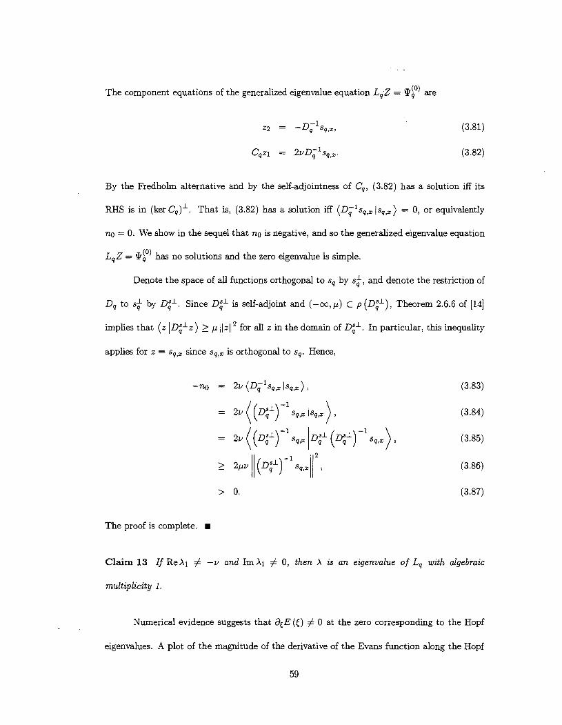
Numerical evidence suggests that deE (J) # 0 at the zero corresponding to the Hopf
eigenvalues. A plot of the magnitude of the derivative of the Evans function along the Hopf
x Magnitude of Derivative of Evans Function ' 6-
- /
4- 2.8 3 3.2 3.4 3.6 3.8 4 4.2 4.4 4.6 4.8
a
Figure 3.10: The magnitude of the derivative of the Evans function along the Hopf bifurcation
curve.
bifurcation curve is shown above. Our claim then follows since the order of the zero is equal
to the algebraic multiplicity of the eigenvalue [I]. Moreover, the normalization constant is
always well defined by Theorem 1.1 of [9].
The operators which spectrally project onto the active space Xq and the stable space
Xi are given by
respectively, where I is the identity operator.
Because the spectrum of the linearized operator is not contained in any sector of the
complex plane, Lq generates only a Co semigroup Sq ( t ) . However, because u (Lq) \{Ao, XI, Az)
is a strict subset of the left-half complex plane, the restriction of Lq to X; enjoys the following
estimate. See Proposition 4.1 of [ll] for details.
Lemma 14 Each operator Lq generates a Co semigroup Sq which satisfies
for some constant cs 2 1, for all Z E X;, and for all t 2 0. The constant cs is chosen to be
independent of q. Thus the Semigroup condition is satisfied.
We end this section with the following lemma.
Lemma 15 If y E (1, dm) and Re Xl # -v and Irn XI # 0, then (I!$ lPF)t ) = 0 for
j , k = 1,2.
Proof. Because the PNLS is invariant under spatial translations, it suffices to show
that ($4 1 9f)t ) = 0 for q = 0. For notational convenience, denote P = ( P f') . q=o
Now, L (3.64) is an even operator in the sense that it is invariant under the reflection
x - -x. So, by replacing x with -x in the eigenvalue equation
we obtain
L (x) @ (-2) = X P (-2) (3.92)
Adding and subtracting (3.91) and (3.92) yields
L (2) ( P (2) + P (-x)) = X ( 9 (x) + P (-2)) , (3.93)
L (x) ( 9 (x) - 9 (-x)) = X ( 9 (x) - P (-x)) (3.94)
respectively. By Claim 13, X has algebraic multiplicity 1 and so it is associated with only one
linearly independent eigenfunction. Because \E (x) - 9 (-x) and \E (x) + \E (-x) are linearly
independent, one of these functions must be zero, and so 9 is either even or odd. By the
expressions (3.76,3.77) for the adjoint eigenfunctions, this is also true of 9t.
We remark that the numerical computations from [6] show that \EF) for q = 0, j = 1,2,
is even.
Functions of opposite parity are mutually orthgonal since, if A is odd and B is even,
we have
To prove our lemma, then, it is sufficient to show that, for functions of definite parity, differ-
entiation changes parity. If A is odd, then
A' (-x) = dA (-X) =- dx aA(-x) - _-- dA (x) a(-x) a(-x) ax ax - A' (4 7
and so A' is even. Similarly, if B is even, then B' is odd.
The Nonlinear Term We compute the nonlinear term N, (3.11) by computing each of the
terms on the right-hand side of
as follows. Denoting the components of Y as Y = (yl, yz)t, direct substitution of Q, + Y =
(s, + yl, ~ 2 ) ~ into F (3.38) yields
As Qq is a stationary solution of the PNLS for all q, then
Finally, direct multiplication of L, (3.64) by Y yields
Substituting these expressions into (3.98), as well as applying the identity
which arises from (3. loo), we obtain
where
Observe that N2 and N3 are bilinear and trilinear in each of their arguments respectively. For
3.3 The Correction Terms
In this section, we determine the correction terms
so that the Quasi-Invariant Manifold condition is satisfied with q- = r4:
T h s is necessary so that W will decay to 0 ( r4) which in turn is necessary for transforming
the evolution equation for r into Poincare normal form in the asymptotic state. As noted
earlier, we demand that Rfk) and Rfkl) depend only on the anchor point and not on q.
Moreover, we impose the same condition
as was imposed on the residual term W.
We impose the following symmetry conditions on Rfk) and Rfk') to ease our calcula-
tions.
(S l ) Rf4, Rfk') is symmetric with respect to the interchange of any two indices.
(3) - O.kl) ( ' ) = P a n d R b -Rb , (S2) Denote = 2 and 5 = 1. Then, Rb
b b - p. Note that, under these conditions, Rr2) is real since Rf 2, = R(~') and R(~ ' ) -
We calculate the terms comprising (3.109) as follows. Recall from (3.59) that
First, multiplying Lb (3.64) by R(b,r) (3.59) yields
Next, by direct substitution of R, (3.59) into Nb (3.104) and using the bilinearity and trilin-
earity of N2 (3.105) and N3 (3.106) respectively,
where
Next, direct differentiation of (3.58) yields
where we have used the identity Q , , = 8p) (3.69) and applied the symmetry conditions
(Sl,S2). Substituting these expressions for apj@, into I I (b , r ) (3.21) then yields
where we have used the orthonormality condition (3.80) and Lemma 15. The inverse of Il(b,r)
Finally, substituting F (Q4) = 0 and W = 0 into wb ( r , W) (3.24) yields
where we have used the relation
Substituting (3.119) for II&, (3.111) for R(b,,), and (3.113) for Nb (R(b,,)) then yields
and, for j = 1,2,
where we have introduced the constants
which are independent of b due to the invariance of the PNLS under spatial translations.
Collecting all of the above expressions (3.112,3.113,3.116,3.117,3.122,3.123), we substitute
into the Quasi-Invariant Manifold condition (3.109) and group the 0 (r2) and 0 (r3) terms
to obtain
where
Applying the symmetry conditions (S1 ,S2), we obtain
where
Both the R's and U's lie in the decay space X;, so the R's are s o h lble provided the
operators (Lb - p) are boundedly invertible on X;. The restriction of Lb to X; has the
spectrum
(3.134)
contained in {z E (C IRe z 5 -k). Thus, by a slight generalization of Lemma 4.2 from [ll],
(Lb - z)-I exist and are uniformly bounded on {z E (C (Rez > -6 > -k). Because the reso-
nances p lie in {z E (C [Re z > -d > -k), the R's are solvable.
Lemma 16 By choosing the correction t e r n R:) and RF) as
where
R,, Component 1
0.015 I
Real Part 0.01 - - - lmag Part
0.005 -
-0.005 - \ I
\ I \ I - -0.01 - "
-0.015 - - -0.02 I I I 1 I I I I I
-25 -20 -15 -10 -5 0 5 10 15 20 25
R,, Component 2 . .
0.03 - I I I I I I I - Real Part - - lmag Part
0.02 - -
0.01 - -
-0.01 -
-25 -20 -15 -10 -5 0 5 10 15 20 25
Figure 3.11: Graph of the manifold correction term RI1 for y = 2.4 and a = 2.8.
and
/-Ljk Xj + X k ,
= X j + X k + X l . pjkl -
the Quasi-Invariant Manifold condition is satisfied.
3.4 The Evolution Equations
In t h s section, we compute explicit expressions for the evolution equations (3.23,3.27)
for p and W. This primarily involves computing explicit expressions for w i (W) (3.24) and
68
R,, Component I
0.015 - - - h a g Part - 0.01 - -
0.005 - -
-0.005 -
-0.01 - -
-25 -20 -15 -10 -5 0 5 10 15 20 25
RI2 Component 2
0.03 I I I I I I I
- Real Part 0.02 - - - h a g Part - 0.01 - -
-0.01 - -
-0.02 - - -0.03 - -
Figure 3.12: Graph of the manifold correction term RI2 for 7 = 2.4 and a = 2.8.
Rb (W) (3.28). We then obtain the mild solution (2.74) for W. Lastly, we transform the
evolution equation for r into Poincare normal form which analytically exhibits the Hopf
bifurcation. In particular, we shall show that the coefficient q of the cubic term in the
Poincarb normal form has positive real part at criticality, and this implies that the Hopf
bifurcation is supercritical.
Most of the following calculations have already been performed in Section 3.3.
The Evolution Equations Recasting wb (r , W) (3.24) as
where
Gjb (r, W) = wb (r , W) - wb (r , 0)
we substitute the expressions (3.122,3.123) for the components of wb (r, 0) to obtain
and, for 3 = 1,2,
where
Also, the components of Zb (p, W) (3.25) are given by
The evolution equation (3.23) for q,t is thus explicitly given by (to leading order)
and ~ j , ~ by
Recasting ab ( r , W ) (3.28) as
where
Also, &, (p, W ) (3.29) is given by
The evolution equation (3.27) for W is thus given by
which posesses the mild solution
W ( t ) = S ( t - t b ) W b + S (t - r ) Gb (7) dr , (3.156)
where the "forcing term" Gb is given by
G(T) Ob (r (T) 0) + f i b (1 (7) , W (7)) + gb (P (7) , W (7)) (3.157)
and Wb - W (tb) is the initial residual with respect to the anchor point b.
The Hopf Bifurcation The evolution equation for rj is given by (3.149):
where it will be shown in Section 3.5 that Zb (r, W) is 0 ( I T / w, w2) and Zb (p, W) is 0 ( ( q - bl).
It will also be shown in Section 3.5 that, in the asymptotic state wherein w is 0 ( r4) , zb (r, W)
and Zb (p, W) are also 0 (r4) . Thus, in the asymptotic state, all terms in (3.149) up to 0 (r3)
are explicitly given. Defining
we rewrite (3.149) as
hkl k - l r,t=k+ C z r r + o ( T ~ ) .
2<k+1<3
We now apply Lemma 3.6 from [12], which we restate below, to transform the evolution
equation (3.166) for r into the Poincari! normal form for the Hopf bifurcation.
Lemma 17 The equation (3.166) with X = X (y), Re X (7,) = 0, Im X (7,) > 0, and hkl =
hkl (y), can be transforned by the invertible parameter-dependent change of complex coordi-
nate:
with jzl = 0 into an equation with only the resonant cubic tern:
for all y such that ly - y,l is suficiently small. hrthermore,
which, at the critical bifurcation value y,, reduces to
If Re q < 0, the Hopf bifurcation is supercritical; otherwise, the Hopf bifurcation .ts subcritical.
The coefficient q, of the cubic term was numerically computed along the Hopf bi-
furcation curve for a E (2.8,4.9) according to (3.170). These computations were performed
using Matlab R13. The most challenging aspects of this computation were the numerical
determination of the Hopf eigenfunction P (3.71) and the correction terms R f k ) (3.137) and
R f k ' ) (3.138). Using results from 161, the Hopf eigenfunction was numerically computed as a
linear combination of Dirichlet expansions on the stable manifold of the associated linearized
eigenvalue problem. The corresponding Evans function plays a key role in this computation,
yielding the Hopf eigenvalues as its zeros and the coefficients used in the linear combination.
See [6] for details. On the other hand, the computation of the correction terms involved
implicitly solving ODES of the type
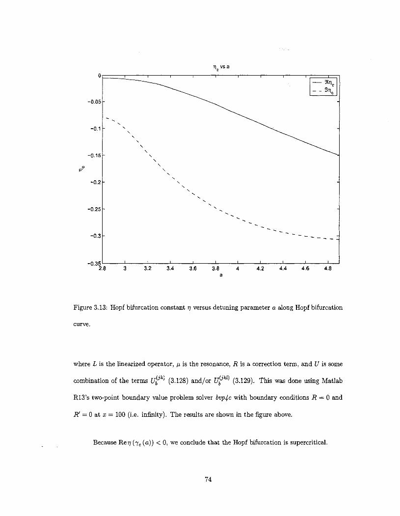
Figure 3.13: Hopf bifurcation constant 7 versus detuning parameter a along Hopf bifurcation
curve.
where L is the linearized operator, p is the resonance, R is a correction term, and U is some
combination of the terms ufk) (3.128) and/or ufkL) (3.129). This was done using Matlab
R13's two-point boundary value problem solver bvp4c with boundary conditions R = 0 and
R' = 0 at x = 100 (i.e. infinity). The results are shown in the figure above.
Because Re 7 (yc (a ) ) < 0, we conclude that the Hopf bifurcation is supercritical.
3.5 Bounds on the Residual Term
From the mild solution (3.156) for W, we obtain the estimate (3.234) for W valid for
the current anchor point b. This estimate shows that control of W is lost after a finite time
period, and this is caused by the secular growth in Sb (3.154). We remove this secularity in
the following section by rechoosing our anchor point as b* in such a way that W E Xi. This
is done by Theorem 18. Lastly, we show that by appropriately choosing the fixed time length
At in which each anchor point is used (see 3.262), the oscillatory solution will approach and
remain near the manifold under suitable initial conditions.
Introduction Fix the anchor point at b on the time interval [tb, td) and denote the h a l value
of q on [tb, td] by d. Also denote w = IIWIIH1, and the initial and h a l values of w on [tb, td]
by wb and wd. The following equations then hold:
The following control quantities play prominent roles in our analysis. The quantity
is the total length of time in which the anchor point b has been in use. The quantity
controls the distance between the manifold position parameter q and the anchor point b, the
quantity
controls the amplitude of the oscillating solution, and the quantity
controls the size of W. W will decay exponentially in accordance with the semigroup decay
estimate (3.90), so the purpose of the exponential factor ek(e-tb) in (3.176) is to compensate
for this decay.
Apply the triangle inequality and the semigroup decay estimate (3.90) to the mild
solution (3.156) for W to obtain
where gb ((GbllH1. A bound on Gb is obtained in the next section, which will then be used
to bound W .
Bound on the Forcing Term The goal in this section is to obtain a bound on the "forcing
term" Gb (3.157). The constant
is chosen for convenience to facilitate our computations. We shall frequently make use of this
fact about the = H1 (R) norm:
and we shall frequently use inequalities like
r + r2 + . . . 5 2r, r small (3.180)
to dismiss the higher order terms in r . In particular, take note of the factor 2 on the right-hand
side of this inequality.
Bounds on Ob (r, 0) and f i b (r, W ) are obtained as follows. All anchor point dependent
quantities such as the linearized eigenfunctions qf) and the correction terms ~ f ~ ) have norms
which are anchor point i n d e p e n d e n t because the PNLS is invariant under spatial translations.
Moreover, the nonlinearity in the PNLS is polynomial in nature, whch means that these
nonlinearities satisfy some type of (bi- or tri-) linearity property. In particular, all the 0 (r4)
terms appearing in Sections 3.3 and 3.4 arise from Nb (R,) and therefore satisfy bounds like
1 1 All Hl 5 c lr14 for some constant c which is anchor point i ndependen t . It therefore follows
from the Quasi-Invariant Manifold condition that
for some constant cn i n d e p e n d e n t of b. As for fib (r, W), let us estimate each of the terms
appearing in the right-hand side of (3.152). First, applying the triangle and Cauchy-Schwarz
inequalities to the spectral projection operator nb (3.89) yields
for any A, and so
Also, by direct substitution of Nq (3.104) in Zq (3.153) and the bilinearity and trilinearity of
N2 (3.105) and N3 (3.106) respectively,
Next, the components of n;Y(b,r) are obtained by applying the spectral projection operator
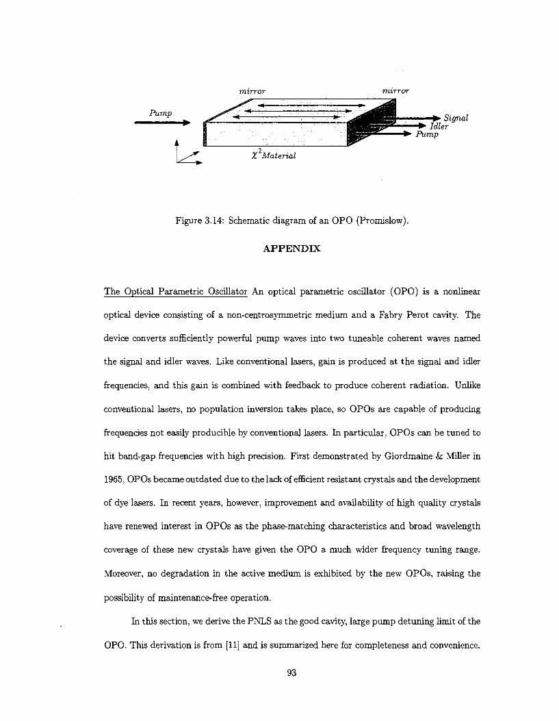
T; (3.89) on the derivatives of @, (3.116,3.117):
Finally, llSb (r, W) 1 1 is obtained by substituting wb (r, W) (3.24) and subsequently lI(alr)
(3.119) into S b (r, W) (3.142), and then applying the estimate (3.186) for sq:
Applying the above estimates to f ib (r , W) (3.152), we obtain
where c~ - max { (1 + 3ci) 2c;, (1 + 3 4 ) ~ C Q , 4c;, 4~;).
Bounds on q,t and Sb (p, W) are obtained as follows. Applying the triangle inequality
to (3.19) yields
Let us estimate each of the terms on the right-hand side. As Qq is a stationary solution of
the PNLS for all q, then F (Qq) = 0 for all q, and so
Next, by the expression (3.64) for Lq, Lq - Lb is a multiplicative operator satisfying the bound
llLq - Lbll,,H1 5 C$ I!? - bl, and so
Next, by direct substitution of R(b,T) + W into Nq (3.104) and the bilinearity and trilineary
of N2 (3.105) and N3 (3.106) respectively,
Finally, multiplying Lq (3.64) by Rp (3.111) and applying the eigenvdue equation L ~ P ~ ) =
A .*Ci) 3 Q ,
while, by direct substitution of dqQp (3.116), arjQp (3.117), and rj,t (3.149),
Therefore the fourth term on the right-hand side of (3.193), which we denote by s4, satisfies
Applying the above estimates to S b (3.193), qrt (3.148), and r,t (3.149) then yields
. .
where c, - max ( 2 4 + 2 4 , 2cq, 8~ ; , 84} . We further combines these estimates as
where we have used the fact that Iq,t] and IrYt - rAl obey the same estimate.
Control of Sb and q,t by the estimates (3.205,3.206) is lost when ~ ( 4 ) grows too large.
We therefore impose the constraint
which restricts the possible size of At, thereby bounding Sb and q,t as
where cqs -- max {4c,, 2c, (1 + 2c,)). We further impose the condition
which restricts the initial size of the residual to obtain
~ ( 9 ) by its definition (3.174) then satisfies the estimate,
2 < 2cqs ( ~ ( ' 1 ) At,
which may be applied to (3.21 1) to obtain
. -
Lastly, a bound on & (p, W) is obtained as follows. Applying the triangle inequality
to (3.154) yields
and subsequent application of the above estimates yields
With the bounds (3.181,3.192,3.217) for !db (W), fib (r, W), gb (q, W) in hand, the
"forcing term" Gb (3.157) satisfies the bound
ge (7) 5 c, ((T('))~ + w ( T ) T(') + (T(')) A t ) , (3.220)
where c, = c~ max icn, 2cii, cF).
So long as the constraints ~ ( 9 ) 5 & (3.207) and w < cs (T('))~ (3.210) hold, then
the estimates 1q.t 1 < 2cq, (T(')) (3.212) and ~ ( 9 ) < 2cqs (T(')) A t (3.214) also hold. On the
other hand, if the estimate (3.214) holds, then the constraint (3.207) also holds if
2 1 2cqs (T(')) At < 7, (3.221)
4%
It is thus self consistent to replace the constraint (3.207) with the constraint (3.221), and we
do so. Lastly, we rewrite (3.221) as
where ct - (8c~cqS)-'.
Residual Decay Estimates We assume that the constraints (3.210,3.222) hold, and we apply
the bound (3.220) for Gb to the estimate (3.177) for W to obtain
t
w ( t ) 5 cse -k( t - tb ) wb + q,, / e-k(t-T) ( W ( T ) T(' + (~( '1) ( 1 + A t ) ) d ~ . (3.223) t b
Replacing t with 0, multiplying by ek(e-tb), and taking the supremum over 8 E Itb, t d ) , (3.223)
becomes
Since
and
(3.225) may be rewritten as
T ( W ) 5 cgwb + q,,
where
92 ( t ) - k-' (en - 1) ( I + t ) .
Note that y2 is a strictly increasing function. Upon solving for T(w) , we obtain
which, by inserting T ( ~ ) (3.176), yields the decay estimate
Because control of wd by (3.232) is lost when At = c;' ( ~ ( ' 1 ) -', we impose the additional
constraint
so that the denominator in (3.232) is uniformly bounded away from zero. It is clear that this
2 constraint is always more exigent than At 5 ct ( ~ ( ' 1 ) - (3.222) for T(') sufficiently small, and
so we hereby replace that constraint with this one. With this constraint, (3.232) becomes
Moreover, by replacing At with t - tb and substituting y2 (3.230), we obtain the residual
decay estimate for general time t:
+2&k-'
3.6 The Reanchor Method
The evolution equations (3.148,3.149,2.73) for p and W remain valid so long as the
secular term Sb (3.19) remains sufficiently small. When this is no longer true, we rechoose
the anchor point to remove this secular growth. Moreover, this new anchor point b* is chosen
so that the new residual lies in X;. Theorem 18 will show that such a choice exists and is
unique, provided that q is sufficiently close to the old anchor point b and provided that W is
sufficiently small. The price of reanchoring is jump discontinuities in both q and W wherein W
could in principle increase, yet we will show that the residual decay estimate (3.234) controls
this possible growth provided that At, the length of time in which each anchor point is used,
is suitably long. The residual decay estimate (3.234) is the key estimate which allows us to
determine such a At so that secular growth is controlled and removed. Lastly, we will show
that after an initial transient stage wherein the residual decays, the residual will remain small
for all time and so our solution remains close to the manifold for all time.
The Reanchor Method Again, fix the anchor point at b on the time interval [tb, td) and denote
the ha1 value of q on [tb, td] by d. Let us introduce the term
and rewrite the decomposition (3.63) for Z as
a
When reanchoring, Z may be decomposed as either Z = + Wd with respect to the old
- a
anchor point b, where Ed E X;, or as Z = Q((*,=) + Wb- with respect to the new anchor point
b', where b' is to be determined so that Eb* E X;. In particular, note that E d E x?)'
and Eb* E x!!)'. Reanchoring introduces a jump discontinuity in both q and W wherein q
jumps from d to b* and jumps from Ed to Eb.. Equating these two decompositions and
solving for Eb*, we obtain
- R- = Ed + O(d,,) - Q(b*,,, .
a
Since Wp E x:?~, then
( E d + G(d,=) - &P,,) /pt) = 0. (3.240)
Given d and k, the following theorem shows that there exists a unique b' such that (3.240)
is satisfied. In addition, this theorem gives an estimate on the jump discontinuity in q when
reanchoring.
Theorem 18 Express & = GdZb for some scalar Gd 2 0 and function Zb E xjO)' satisfying
l/ZbllH1 = 1. For Gd suficiently small, there exists a unique smooth function 'H : IRf - IR such that, by choosing b* = d + 'H (Gd), (3.240) is satisfied. Moreover, the estimate
Id- b*( 5 +GdId - bl (3.241)
holds for some constant +.
Proof. The equation (3.240) is equivalent to r = 0, where
r has a root at (Gd, b*) = (0, d) and r,b* (0, d) = - 1 + 0 ( r ) which is 0 (I) , so the implicit
function theorem guarantees the existence of a smooth function 'H such that b* = d +'H (Gd).
Moreover, since r,Gd (0, d) is 0 (d - b), the implicit function theorem implies that J'H' (0) I is
0 (d - b) also. The estimate (3.241) then follows from the Mean Value Theorem.
Estimates on the Reanchor Jump Discontinuities Since N2 (3.105) and N3 (3.106) are bilinear
and trilinear with respect to their arguments respectively, they are also continuous maps from
H' x H1 and H1 x H1 x H 1 to H1 respectively. Moreover, Lb (3.64) and ~ f ) (3.68,3.71)
are continuous with respect to b, and so it follows that R f k ) and R f k l ) are continuous with
respect to b as well. This continuity property plays a crucial role in-the computation of the
reanchor jump estimate, as we shall see forthwith.
When reanchoring, Z may be decomposed as either
with respect to the old anchor point b, where Wd E X b , or as
with respect to the new anchor point b*, where Wb- E Xb; . Equating these two decompositions
and solving for Wb- yields
Apply the triangle inequality to obtain
Since Q,, R::!~), R[&, R::!~) are continuous with respect to their arguments,
andsince Ib-b*l = l b - d + d - b * l < I d - b l + I d - b * l ,
Finally, inserting the estimates (3.241) for Id - b*l yields
which, by inserting the estimate (3.214) for Id - b/ and using the fact that Gd = R r ) + RP I I becomes
wag < wd + CJ (T(')) At, (3.254)
where CJ - (8c;c' + 2cq) 2cq,. This estimate shows that w could in principle increase when
reanchoring, yet we will show in the next section that the residual decay estimate (3.234)
controls this possible growth provided that At, the length of time in which each anchor point
is used, is suitably long.
The Iterations We now investigate two states in which, for some m to be determined, either
wb E ( m ( T ( ' ) ) ~ , CJ (T(')12) or wb E 0, m T(') respectively. These states are c d e d the [ ( )41
initial transient and asymptotic states. We will show that w decreases on the whole in the
initial transient state in the sense that wb- < wb, while w remains small in the asymptotic
state. Moreover, we will show that we can take At = k-' In (h;' (4cs + 4e, + 2kcJ) + 1) and
m = y2 ( A t ) for some h, < 1.
Inserting the residual decay estimate (3.234) into the reanchor jump estimate (3.254)
yields
wb- 5 2e-'at ( c ~ wb + e, (T(')) y2 ( a t ) ) + CJ ( ~ ( ' 1 ) ~ At (3.255)
This inequality holds so long as the two constraints wb < CJ ( T ( ' ) ) ~ (3.210) and A t <
(e,T('))-' (3.233) holds. To continue using (3.255), we must rechoose our anchor point
before either of these constraints fail.
4 Initial Tkansient State In the initial transient state wherein wb E T(')) , CJ ( ~ ( ' 1 ) ~ ) ~ we
further impose the constraint
on A t and apply it and substitute the expression (3.230)
gz ( a t ) = k-' (ekAt - 1 ) ( 1 + a t )
into (3.255) to obtain
= h ( A t ) wb, (3.260)
where
We now choose the h e d length of time At in which the current anchor point b is used such
that h ( A t ) z hm for some hm < 1. The choice
yields
hm = h ( A t ) ,
- - ~ ( C S f h ) h m f kc^ h m 4 (cs + c,) f 2kcj + hm 4 (cs + h ) + 2kcj
and (3.260) thus becomes
We further choose
so that the constraint (3.256) is automatically satisfied by virtue of the fact that wb E
(m ( T ( ' ) ) ~ , cs It remains to show that our choice of At also satisfies the constraint
(3.233), but this is easily satisfied if we demand that T(') satisfy
For what initial conditions on r and w does (3.269) hold? We again transform the
evolution equation (3.166) for r into Poincar6 normal form, but this time we retain the higher
order terms Gb + Zb since we're working in the initial transient state:
Express v = Ivl eis and gather real parts.
Applying the bounds (3.142) and (3.219) for Sb (r , W) and Eb (p, W) then yields
lvl, = (ReX) Ivl + (Req) lv3 + ~ C $ W T ( ' ) + 4c;w2 + c*cz ( ~ ( ' 1 ) ~ At + 0 (lv14) . (3.272)
2 Finally, applying the constraints w < cs (T(')) (3.210) and the choice (3.222) for At, we
obtain
1 ~ 1 , ~ = (Re A) lvl + (Req) lu13 + 4 c & , ( T ( ' ) ) ~ + 0 (1v14) . (3.273)
Choose cs is sufficiently small such that Req + 4c& < 0. Then I T ( will always satisfy the
bound
if 17.1 is initially small enough, while Iri will eventually satisfy this bound if Irl is initially
large provided the constraint (3.269) initially holds. Note that, since w decays, Irl actually
approaches J- Re X /Re 7 . In any case, for Re X and cs sufficiently small, the constraint
(3.269) always holds.
We have thus proven that, if wb E ( m ( T ) ~ , c ( T ' ) ~ ) and At is chosen as in
(3.262), the residual decays on the whole in the sense that wb* 5 h,wb. Moreover, we have
determined the appropriate initial conditions under which our analysis holds. In particular,
the solution must be close enough to the manifold and the oscillation amplitude must be small
enough such that the residual satisfies w (0) < ca ( ~ ( ' 1 ) ~ (3.210) and such that the condition
(3.269) holds.
The residual will continue to decay until wb E at which point the system
enters the asymptotic state.
Asymptotic State In the asymptotic state wherein wb E , we choose At as in
(3.262):
Since 32 (At) = rn and wb 5 m (T('))~, (3.255) then becomes
where h is given by (3.261) as before. Since h (At) = h,, we have
We have thus proven that, if wb E 0, m T(') and At is chosen as in (3.262), then [ ( 141
also. In conjunction with the decay estimate (3;234), this shows that
w ( t ) 5 2 (cs + G) ( m ( T ( ' ) ) ~ ) (3.279)
for all time t in the asymptotic state.
3.7 Conclusion
We conclude our thesis with the following theorem which summarizes our results.
Theorem 19 Consider the vectorized parametrically-forced nonlinear Schrodinger equation
Provided that Re X and w are suficiently small, the PNLS posesses the solution
for each jixed anchor point b, where
Here, Qq is the stationary pulse solution, '2:) are the linearized eigenfunctions, and RFk)
and RFk') are the anchor-point dependent comction terms. The manifold parameters satisfy
the evolution equations ( in the asymptotic state)
where X j are the Hopf eigenvalues, and yjkl and yjklm are anchor-point independent numbers.
The residual term W satisfies the condition
and the bound
w ( t ) j 2e-k('-'b) (cswb + c, ( T ( ' ) ) ~ yyz ( t - t b ) ) (3.286)
with y2 ( t ) G k-' (ekt - 1 ) ( 1 + t ) . Moreover, one can use each anchor point for an 0 ( 1 ) time
period and rechoose the anchor point thereafter according to Theorem 18 such that, in the
initial transient state, wb. < hmwb for some f i e d constant h, < 1 and, in the asymptotic
state, w 5 mb for some 0 ( 1 ) constant m.
2 X Material
Figure 3.14: Schematic diagram of an OPO (Promislow).
APPENDIX
The Optical Parametric Oscillator An optical parametric oscillator (OPO) is a nonlinear
optical device consisting of a non-centrosymmetric medium and a Fabry Perot cavity. The
device converts sufficiently powerful pump waves into two tuneable coherent waves named
the signal and idler waves. Like conventional lasers, gain is produced at the signal and idler
frequencies, and this gain is combined with feedback to produce coherent radiation. Unlike
conventional lasers, no population inversion takes place, so OPOs are capable of producing
frequencies not easily producible by conventional lasers. In particular, OPOs can be tuned to
hit band-gap frequencies with high precision. First demonstrated by Giordmaine & Miller in
1965, OPOs became outdated due to the lack of efficient resistant crystals and the development
of dye lasers. In recent years, however, improvement and availability of high quality crystals
have renewed interest in OPOs as the phase-matching characteristics and broad wavelength
coverage of these new crystals have given the OPO a much wider frequency tuning range.
Moreover, no degradation in the active medium is exhibited by the new OPOs, raising the
possibility of maintenance-free operation.
In this section, we derive the PNLS as the good cavity, large pump detuning limit of the
OPO. This derivation is from [ll] and is summarized here for completeness and convenience.
93
. .
We consider the degenerate OPO near the single-mode resonances at the fundamental
and second harmonic of a planar cavity in the good cavity limit. The mean-field model for
dimensionless signal and pump field envelopes are respectively denoted by u and v and are
governed by the equations
where A1 and A2 are the cavity detuning parameters, p is the diffraction ratio between the
signal and pump fields, cr is the pumpto-signal loss ratio, and s represents the pumping
term. See [18, 191. The OPO exhibits subcritical bistable behaviour for both front and
solitary wave solutions, but we investigate this behaviour for only solitary wave solutions in
the large pumpdetuning regime for which >> 1. Rewriting (3.288) as
1. = A?' (s - u2) - iv,
we assume s = 0 (lA21), u = 0 (m), and v = 0 (I) , as well as neglect the left-hand side
terms to obtain
For consistency with (3.287,3.288), we also require that \All >> a / /A2 ( . Inserting (3.290)
into (3.287) yields the PNLS equation
Rescaling as u = m4, a = A, > 0, and y = AT'S, we obtain the focusing PNLS
where y is the pump strength and a is the detuning parameter.
94
REFERENCES CITED
1. J Alexander, R Gardner, CKRT Jones. A Topological Invariant Arising in the Stability
of Travelling Waves. J. Reine Angew. Math. 410, 167-212 (1990).
2. N Alexeeva, I Barashenkov, D Pelinovsky. Dynamics of the Parametrically Driven NLS
Solitons Beyond the Onset of the Oscillatory Instability. Nonlinearity 12,103-140 (1999).
3. 1 Barashenkov, M Bogdan, V Korobov. Stability Diagram of the Phase-Locked Solitons
in the Parametrically Driven Damped Nonlinear Schrodinger Equation. Europhys. Lett.
15, 113-118 (1991).
4. P Bates and CKRT Jones. Invariant Manifolds for Semilinear Partial Differential Equa-
tions. Dynamics Reported 2, 1-38 (1989).
5. M Bondila, I Barashenkov, M Bogdan. Topography of Attractors of the Parametrically
Driven Damped Nonlinear Schrodinger Equation. Physica D 87, 314-320 (1995).
6. PC Chang. MSc Thesis, Simon Fraser University, (unpublished, 2000).
7. LY Chen, N Goldenfeld, Y Oono. Renormalization Group and Singular Perturbations:
Multiple Scales, Boundary Layers, and Reductive Perturbation Theory. Phys. Rev. E (3)
54, 376-394 (1996).
8. F Gesztesy, CKRT Jones, Y Latushkin, M Stanislavova. A Spectral Mapping Theorem
and Invariant Manifolds for Nonlinear Schrodinger Equations. Indiana University Math
Journal 49, 221-243 (2000).
9. T Kapitula. The Evans Function and Generalized Melnikov Integrals. SIAM J. Math.
Anal. 30, 273-297 (1999).
10. T Kapitula and B Sandstede. Stability of Bright Solitary-Wave Solutions to Perturbed
Nonlinear Schrodinger Equations. Physica D 124, 58-103 (1998).
11. J N Kutz and K Promislow. Bifurcation and Asymptotic Stability in the Large Detuning
Limit of the Optical Parametric Oscillator. Nonlinearity 13, 675-698 (2000).
12. YA Kuznetsov. Elements of Applied Bifurcation Theory, (Springer-Verlag, 1995).
13. YA Li and K Promislow. The Mechanism of the Polarizational Mode Instability in Bire-