Page 1
MODULE 10EXPERIMENTAL MODAL ANALYSIS
Most vibration problems are related to resonance phenomena where
operational forces excite one or more mode of vibration.
Modes of vibration which lie within the frequency range of the operations
dynamic forces, always represent potential problems.
An important property of modes is that any dynamic response (forced or free)
of a structure can be reduced to a response of discrete set of modes.
Page 2
2DOF.SLDASM
DISCRETE SYSTEMS
Page 3
multi pendulum.SLDASM
DISCRETE SYSTEMS
Page 4
1st mode
2nd mode
3rd mode
4th mode
5th mode
LEGO.SLDASM
DISTRIBUTED SYSTEMS
Experimental analysis to follow
Page 5
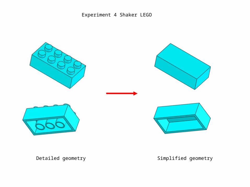
Experiment 4 Shaker LEGO
Page 6
Detailed geometry Simplified geometry
Experiment 4 Shaker LEGO
Page 7
Modulus of elasticity as for the ABS plastic
Material density has been adjusted so that the simplified block have the same mass as real blocks
2.323g 1.261g
Experiment 4 Shaker LEGO
Page 8
The first vibration mode in the direction of excitation
lego cantilever.SLDASM
Note that there are gaps between blocks indicated by red arrows.
Experiment 4 Shaker LEGO
Page 9
pan.SLDPRT
1st mode
2nd mode
3rd mode
4th mode
5th mode
6th mode
DISTRIBUTED SYSTEMS
Page 10
The modal parameters are:
Modal frequency
Modal shape
Modal damping
Modal parameters represent the inherent properties of a structure which are independent of any excitation.
Modal analysis is the process of determining all the modal parameters which is sufficient for formulating a mathematical model of a dynamic response.
Modal analysis may be accomplished either through analytical, numerical or experimental techniques.
EXPERIMENTAL MODAL ANALYSIS
Page 11
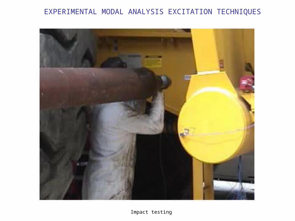
EXPERIMENTAL MODAL ANALYSIS EXCITATION TECHNIQUES
Impact testing
Page 12
EXPERIMENTAL MODAL ANALYSIS EXCITATION TECHNIQUES
Impact testing
Page 13
EXPERIMENTAL MODAL ANALYSIS EXCITATION TECHNIQUES
Impact testing
Page 14
EXPERIMENTAL MODAL ANALYSIS EXCITATION TECHNIQUES
Shaker testing
Page 15
EXPERIMENTAL MODAL ANALYSIS EXCITATION TECHNIQUES
Shaker testing
Page 16
EXPERIMENTAL MODAL ANALYSIS EXCITATION TECHNIQUES
Shaker testing
Page 17
EXPERIMENTAL MODAL ANALYSIS EXCITATION TECHNIQUES
Shaker testing
Page 18
Note:
sine excitation is NOT the only one available
SHAKERS
Shaker can provide both force and base excitation
Page 19
shaker.sldprt
SHAKERS
Page 21
pan.SLDPRT
Mode 1
Mode 2
Shakers
Page 22
Experimental kit to demonstrate modes of vibration of a cantilever beam
Mode 1 3.5Hz
Mode 2 23Hz
Mode 3 63Hz
Mode 4 127Hz
CANTILEVER BEAM EXPERIMENT
Page 23
CA
NT
ILE
VE
R B
EA
M A
NA
LY
TIC
AL
SO
LU
TIO
N
Page 24
cantilever beam MME9500.SLDPRT
This model should give the same results as the experiment in previous slide.
CANTILEVER BEAM NUMERICAL SOLUTION
Page 25
Mode 1 Mode 2 Mode 3 Mode 5
Where is Mode 4 ?
CANTILEVER BEAM NUMERICAL SOLUTION
Page 26
Most common means of Implementing the excitation
Non-attached exciters
Hammers
Pendulum impactors
Attached exciters
Shakers
Eccentric rotating devices
EXPERIMENTAL MODAL ANALYSIS
Hammers
The excitation is transient
The duration and thus the shape of the spectrum of the impact is determined by the mass and
stiffness of both the hammer and the structure. For a relatively small hammer used on a hard
structure, the stiffness of the hammer determines the spectrum.
Page 27
Force excitation time historybase 010.sldprt
Fixed geometry
1000N
Page 28
Force excitation time historybase 010.sldprt
Fixed geometry
500N
500N
Uz Uy
Page 29
Fourier beam.sldprt
-2
-1.5
-1
-0.5
0
0.5
1
1.5
2
0 0.05 0.1 0.15 0.2 0.25
0
0.25
0.5
0.75
1
0 20 40 60 80 100
Response time history
It is not immediately obvious what frequencies are present in the response
Transformation from the time to the frequency domain
(Fourier transformation)
Response spectrum
In the frequency domain it is clear that two frequencies have been excited: 8Hz and 53Hz
Page 30
The Fourier transform is a mathematical operation that decomposes a signal into its constituent frequencies. Thus the
Fourier transform of a musical chord is a mathematical representation of the amplitudes of the individual notes that
make it up. The original signal depends on time, and therefore is called the time domain representation of the signal,
whereas the Fourier transform depends on frequency and is called the frequency domain representation of the signal.
The term Fourier transform refers both to the frequency domain representation of the signal and the process that
transforms the signal to its frequency domain representation.
FOURIER TRANSFORM
Page 31
What is a Fourier Transform?
A Fourier Transform is a mathematical operation that transforms a signal from the time domain to the frequency
domain. We are accustomed to time-domain signals in the real world. In the time domain, the signal is expressed
with respect to time. In the frequency domain, a signal is expressed with respect to frequency.
What is a DFT? What is an FFT? What's the difference?
A DFT (Discrete Fourier Transform) is simply the name given to the Fourier Transform when it is applied to digital
(discrete) rather than an analog (continuous) signal. An FFT (Fast Fourier Transform) is a faster version of the DFT
that can be applied when the number of samples in the signal is a power of two. An FFT computation takes
approximately N * log2(N) operations, whereas a DFT takes approximately N2 operations, so the FFT is significantly
faster.
http://www.ni.com/support/labview/toolkits/analysis/analy3.htm
FOURIER TRANSFORM
Page 32
FOURIER TRANSFORM
Continuous function
Discrete function
Page 34
-30
-20
-10
0
10
20
30
0 0.2 0.4 0.6 0.8 1
0.00
2.00
4.00
6.00
8.00
10.00
12.00
14.00
16.00
0.00 10.00 20.00 30.00 40.00 50.00 60.00
Fourier beam.sldprt
Page 35
Mode 1 4.5Hz
0.22s
Mode 1 26Hz
0.038s
Mode 3 42Hz
0.023s
Mode 4 75Hz
0.013s
Page 36
Fourier beam.SLDPRT
Study 01dt impulse duration 0.0075
Page 37
Study 01dt
Response time history FFT of response time history
Only mode 1 and mode 2 are excited. Larger impulse (longer duration) caused larger displacement amplitude response
Page 38
Fourier beam.SLDPRT
Study 02dt impulse duration 0.05
Page 39
Study 02dt
Response time history FFT of response time history
Only mode 1 is excited. Larger impulse (longer duration) caused larger displacement amplitude response
Page 40
Study 03dt impulse duration 0.0075
Page 41
Study 03dt
Response time history FFT of response time history
Mode 1 and mode 2 are excited.
Page 42
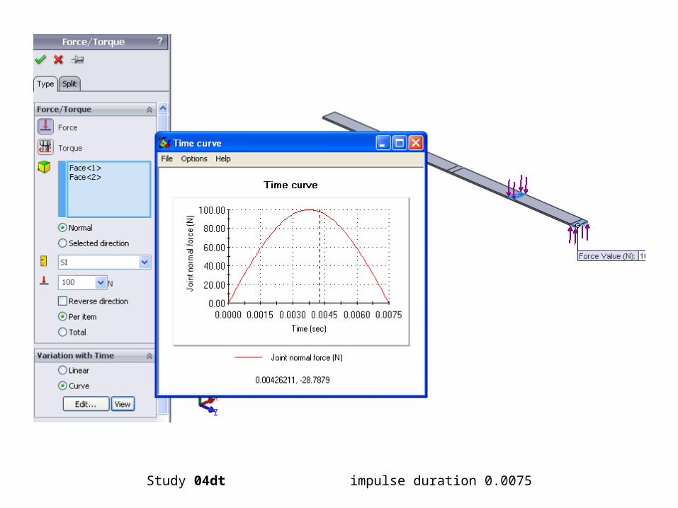
Study 04dt impulse duration 0.0075
Page 43
Study 04dt
Response time history FFT of response time history
Mode 1 and mode 2 are excited.
Page 44
Fourier beam.SLDPRT
Study 05dt impulse duration 0.05
Based on one mode only
1% damping
Page 45
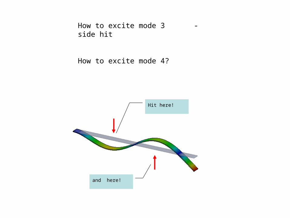
How to excite mode 3 - side hit
How to excite mode 4?
Hit here!
and here!
Page 46
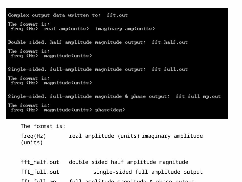
The format is:
freq(Hz) real amplitude (units) imaginary amplitude (units)
fft_half.out double sided half amplitude magnitude
fft_full.out single-sided full amplitude output
fft_full_mp full amplitude magnitude & phase output
Page 47
fourier.exe or fft.exe can be used
Page 48
elipse.sldprt in /vibration experiments
PREPARATION FOR LAB
Page 49
hex.sldprt in /vibration experiments
PREPARATION FOR LAB
Page 50
PREPARATION FOR LAB
tree.sldprt in /vibration experiments