Module 11Module 11Statistics

Andrew JaffeInstructor

StatisticsNow we are going to cover how to perform a variety of basic statistical tests in R.

Note: We will be glossing over the statistical theory and "formulas" for these tests. There areplenty of resources online for learning more about these tests, as well as dedicated Biostatisticsseries at the School of Public Health

Correlation

T-tests

Linear Regression

Logistic Regression

Proportion tests

Chi-squared

Fisher's Exact Test

·

·

·

·

·

·

·

2/31

Correlationcor() performs correlation in R

Like other functions, if there are NAs, you get NA as the result. But if you specify use only thecomplete observations, then it will give you correlation on the non-missing data.

cor(x, y = NULL, use = "everything", method = c("pearson", "kendall", "spearman"))

> load("charmcirc.rda")> cor(dat2$orangeAverage, dat2$purpleAverage)

[1] NA

> cor(dat2$orangeAverage, dat2$purpleAverage, use="complete.obs")

[1] 0.9208

3/31

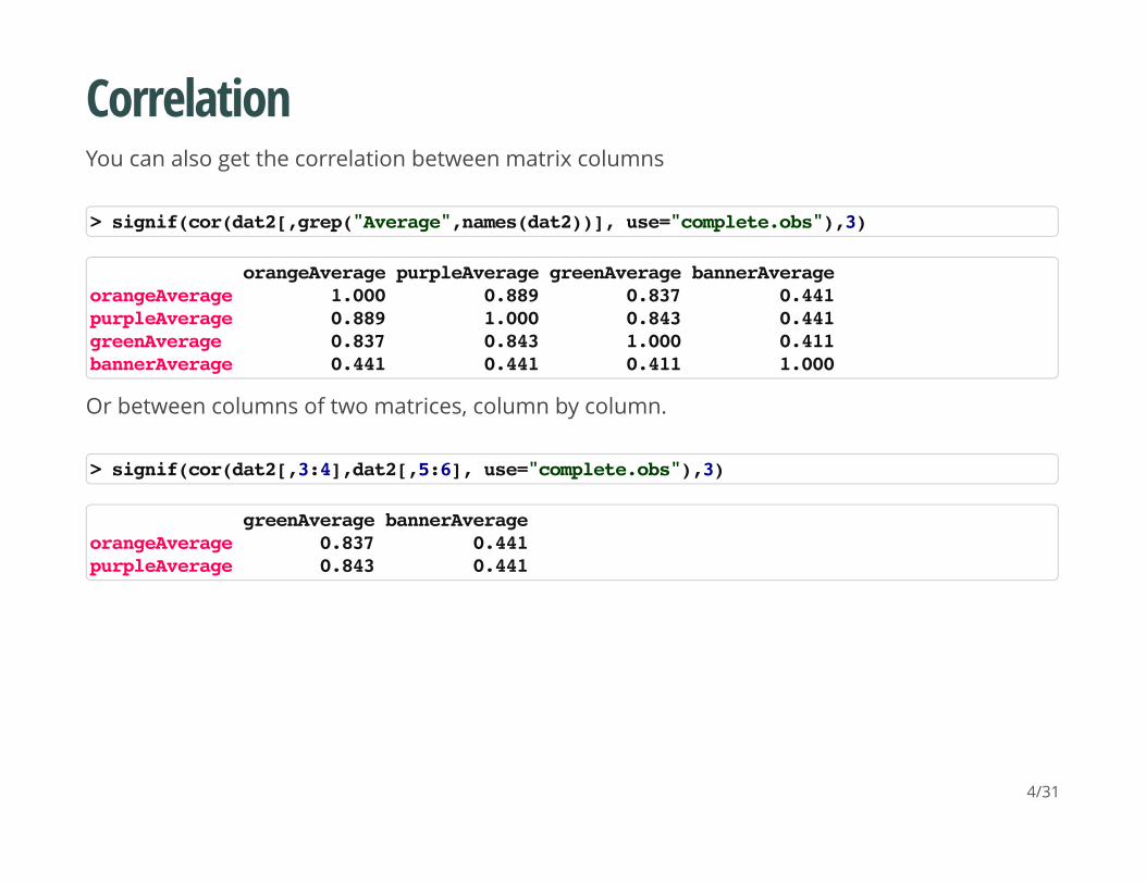
CorrelationYou can also get the correlation between matrix columns

Or between columns of two matrices, column by column.

> signif(cor(dat2[,grep("Average",names(dat2))], use="complete.obs"),3)

orangeAverage purpleAverage greenAverage bannerAverageorangeAverage 1.000 0.889 0.837 0.441purpleAverage 0.889 1.000 0.843 0.441greenAverage 0.837 0.843 1.000 0.411bannerAverage 0.441 0.441 0.411 1.000

> signif(cor(dat2[,3:4],dat2[,5:6], use="complete.obs"),3)

greenAverage bannerAverageorangeAverage 0.837 0.441purpleAverage 0.843 0.441

4/31

CorrelationYou can also use cor.test() to test for whether correlation is significant (ie non-zero). Note thatlinear regression may be better, especially if you want to regress out other confounders.

> ct= cor.test(dat2$orangeAverage, dat2$purpleAverage, use="complete.obs")> ct

Pearson's product-moment correlation

data: dat2$orangeAverage and dat2$purpleAveraget = 69.65, df = 871, p-value < 2.2e-16alternative hypothesis: true correlation is not equal to 095 percent confidence interval: 0.9100 0.9303sample estimates: cor 0.9208

5/31

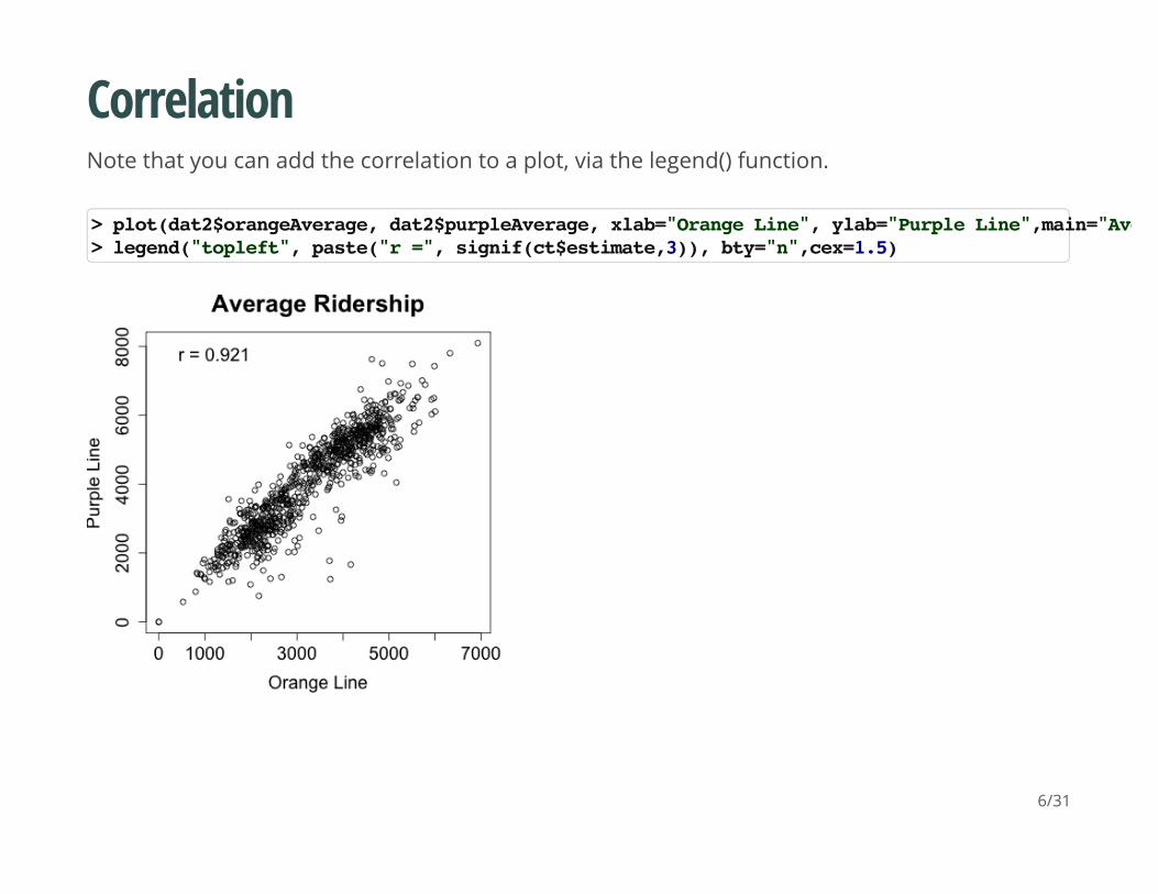
CorrelationNote that you can add the correlation to a plot, via the legend() function.

> plot(dat2$orangeAverage, dat2$purpleAverage, xlab="Orange Line", ylab="Purple Line",main="Average Ridership"> legend("topleft", paste("r =", signif(ct$estimate,3)), bty="n",cex=1.5)

6/31

CorrelationFor many of these testing result objects, you can extract specific slots/results as numbers, asthe ct object is just a list.

> # str(ct)> names(ct)

[1] "statistic" "parameter" "p.value" "estimate" "null.value" [6] "alternative" "method" "data.name" "conf.int"

> ct$statistic

t 69.65

> ct$p.value

[1] 0

7/31

T-testsThe T-test is performed using the t.test() function, which essentially tests for the differencein means of a variable between two groups.

In this syntax, x and y are the column of data for each group.

> tt = t.test(dat2$orangeAverage, dat2$purpleAverage)> tt

Welch Two Sample t-test

data: dat2$orangeAverage and dat2$purpleAveraget = -16.22, df = 1745, p-value < 2.2e-16alternative hypothesis: true difference in means is not equal to 095 percent confidence interval: -1141.5 -895.2sample estimates:mean of x mean of y 2994 4013

8/31

T-testst.test saves a lot of information: the difference in means estimate, confidence interval forthe difference conf.int, the p-value p.value, etc.

> names(tt)

[1] "statistic" "parameter" "p.value" "conf.int" "estimate" [6] "null.value" "alternative" "method" "data.name"

9/31

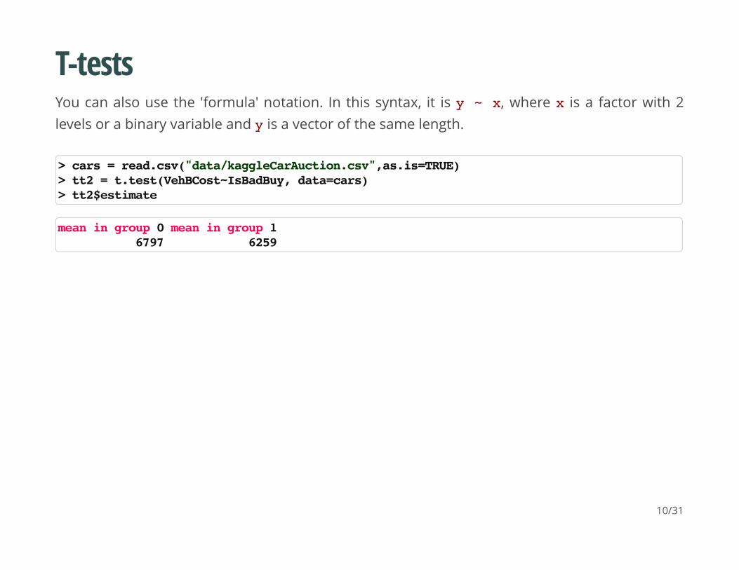
T-testsYou can also use the 'formula' notation. In this syntax, it is y ~ x, where x is a factor with 2levels or a binary variable and y is a vector of the same length.

> cars = read.csv("data/kaggleCarAuction.csv",as.is=TRUE)> tt2 = t.test(VehBCost~IsBadBuy, data=cars)> tt2$estimate

mean in group 0 mean in group 1 6797 6259

10/31

T-testsYou can add the t-statistic and p-value to a boxplot.

> boxplot(VehBCost~IsBadBuy, data=cars, xlab="Bad Buy",ylab="Value")> leg = paste("t=", signif(tt$statistic,3), " (p=",signif(tt$p.value,3),")",sep="")> legend("topleft", leg, cex=1.2, bty="n")

11/31

Linear RegressionNow we will briefly cover linear regression. I will use a little notation here so some of thecommands are easier to put in the proper context.

where:

= α + β +yi xi εi

is the outcome for person i

is the intercept

is the slope

is the predictor for person i

is the residual variation for person i

· yi

· α· β· xi

· εi

12/31

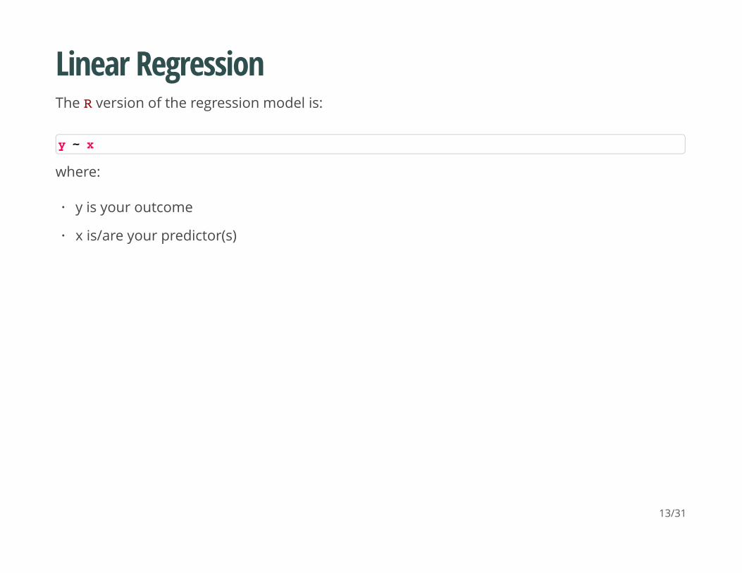
Linear RegressionThe R version of the regression model is:

where:

y ~ x

y is your outcome

x is/are your predictor(s)

·

·

13/31

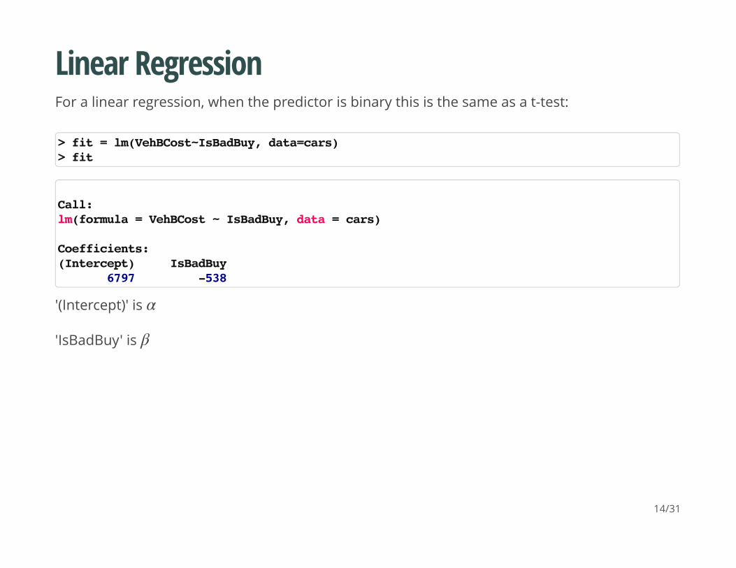
Linear RegressionFor a linear regression, when the predictor is binary this is the same as a t-test:

'(Intercept)' is

'IsBadBuy' is

> fit = lm(VehBCost~IsBadBuy, data=cars)> fit

Call:lm(formula = VehBCost ~ IsBadBuy, data = cars)

Coefficients:(Intercept) IsBadBuy 6797 -538

α

β

14/31

Linear RegressionThe summary command gets all the additional information (p-values, t-statistics, r-square) thatyou usually want from a regression.

> sfit = summary(fit)> print(sfit)

Call:lm(formula = VehBCost ~ IsBadBuy, data = cars)

Residuals: Min 1Q Median 3Q Max -6258 -1297 -27 1153 39210

Coefficients: Estimate Std. Error t value Pr(>|t|) (Intercept) 6797.08 6.95 977.6 <2e-16 ***IsBadBuy -537.80 19.83 -27.1 <2e-16 ***---Signif. codes: 0 '***' 0.001 '**' 0.01 '*' 0.05 '.' 0.1 ' ' 1

Residual standard error: 1760 on 72981 degrees of freedomMultiple R-squared: 0.00998, Adjusted R-squared: 0.00997 F-statistic: 736 on 1 and 72981 DF, p-value: <2e-16

15/31

Linear RegressionThe coefficients from a summary are the coefficients, standard errors, t-statistcs, and p-valuesfor all the estimates.

> names(sfit)

[1] "call" "terms" "residuals" "coefficients" [5] "aliased" "sigma" "df" "r.squared" [9] "adj.r.squared" "fstatistic" "cov.unscaled"

> sfit$coef

Estimate Std. Error t value Pr(>|t|)(Intercept) 6797.1 6.953 977.61 0.000e+00IsBadBuy -537.8 19.826 -27.13 3.017e-161

16/31

Linear RegressionWe'll look at vehicle odometer value by vehicle age:

fit = lm(VehOdo~VehicleAge, data=cars)print(fit)

## ## Call:## lm(formula = VehOdo ~ VehicleAge, data = cars)## ## Coefficients:## (Intercept) VehicleAge ## 60127 2723

17/31

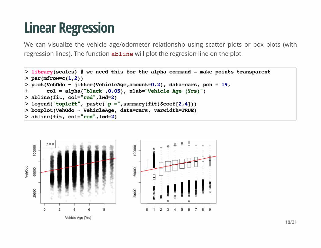
Linear RegressionWe can visualize the vehicle age/odometer relationshp using scatter plots or box plots (withregression lines). The function abline will plot the regresion line on the plot.

> library(scales) # we need this for the alpha command - make points transparent> par(mfrow=c(1,2))> plot(VehOdo ~ jitter(VehicleAge,amount=0.2), data=cars, pch = 19,+ col = alpha("black",0.05), xlab="Vehicle Age (Yrs)")> abline(fit, col="red",lwd=2)> legend("topleft", paste("p =",summary(fit)$coef[2,4]))> boxplot(VehOdo ~ VehicleAge, data=cars, varwidth=TRUE)> abline(fit, col="red",lwd=2)

18/31

Linear RegressionNote that you can have more than 1 predictor in regression models.The interpretation for eachslope is change in the predictor corresponding to a one-unit change in the outcome, holding allother predictors constant.

> fit2 = lm(VehOdo ~ IsBadBuy + VehicleAge, data=cars)> summary(fit2)

Call:lm(formula = VehOdo ~ IsBadBuy + VehicleAge, data = cars)

Residuals: Min 1Q Median 3Q Max -70856 -9490 1390 10311 41193

Coefficients: Estimate Std. Error t value Pr(>|t|) (Intercept) 60141.8 134.7 446.33 <2e-16 ***IsBadBuy 1329.0 157.8 8.42 <2e-16 ***VehicleAge 2680.3 30.3 88.53 <2e-16 ***---Signif. codes: 0 '***' 0.001 '**' 0.01 '*' 0.05 '.' 0.1 ' ' 1

Residual standard error: 13800 on 72980 degrees of freedomMultiple R-squared: 0.103, Adjusted R-squared: 0.103 F-statistic: 4.2e+03 on 2 and 72980 DF, p-value: <2e-16

19/31

Linear RegressionAdded-Variable plots can show you the relationship between a variable and outcome afteradjusting for other variables. The function avPlots from the car package can do this:

> library(car)> avPlots(fit2)

20/31

Linear RegressionPlot on an lm object will do diagnostic plots. Residuals vs. Fitted should have no discernableshape (the red line is the smoother), the qqplot shows how well the residuals fit a normaldistribution, and Cook's distance measures the influence of individual points.

> par(mfrow=c(2,2))> plot(fit2, ask= FALSE)

21/31

Linear RegressionFactors get special treatment in regression models - lowest level of the factor is the comparisongroup, and all other factors are relative to its values.

> fit3 = lm(VehOdo ~ factor(TopThreeAmericanName), data=cars)> summary(fit3)

Call:lm(formula = VehOdo ~ factor(TopThreeAmericanName), data = cars)

Residuals: Min 1Q Median 3Q Max -71947 -9634 1532 10472 45936

Coefficients: Estimate Std. Error t value Pr(>|t|) (Intercept) 68248 93 733.98 < 2e-16 ***factor(TopThreeAmericanName)FORD 8524 158 53.83 < 2e-16 ***factor(TopThreeAmericanName)GM 4952 129 38.39 < 2e-16 ***factor(TopThreeAmericanName)NULL -2005 6362 -0.32 0.75267 factor(TopThreeAmericanName)OTHER 585 160 3.66 0.00026 ***---Signif. codes: 0 '***' 0.001 '**' 0.01 '*' 0.05 '.' 0.1 ' ' 1

Residual standard error: 14200 on 72978 degrees of freedomMultiple R-squared: 0.0482, Adjusted R-squared: 0.0482 F-statistic: 924 on 4 and 72978 DF, p-value: <2e-16 22/31

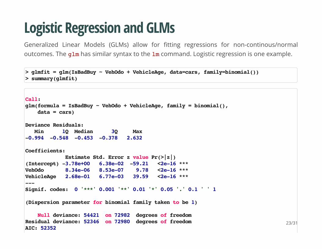
Logistic Regression and GLMsGeneralized Linear Models (GLMs) allow for fitting regressions for non-continous/normaloutcomes. The glm has similar syntax to the lm command. Logistic regression is one example.

> glmfit = glm(IsBadBuy ~ VehOdo + VehicleAge, data=cars, family=binomial())> summary(glmfit)

Call:glm(formula = IsBadBuy ~ VehOdo + VehicleAge, family = binomial(), data = cars)

Deviance Residuals: Min 1Q Median 3Q Max -0.994 -0.548 -0.453 -0.378 2.632

Coefficients: Estimate Std. Error z value Pr(>|z|) (Intercept) -3.78e+00 6.38e-02 -59.21 <2e-16 ***VehOdo 8.34e-06 8.53e-07 9.78 <2e-16 ***VehicleAge 2.68e-01 6.77e-03 39.59 <2e-16 ***---Signif. codes: 0 '***' 0.001 '**' 0.01 '*' 0.05 '.' 0.1 ' ' 1

(Dispersion parameter for binomial family taken to be 1)

Null deviance: 54421 on 72982 degrees of freedomResidual deviance: 52346 on 72980 degrees of freedomAIC: 52352

23/31

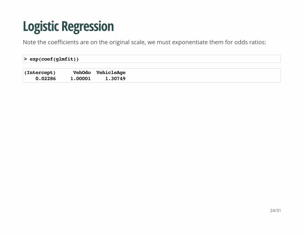
Logistic RegressionNote the coefficients are on the original scale, we must exponentiate them for odds ratios:

> exp(coef(glmfit))

(Intercept) VehOdo VehicleAge 0.02286 1.00001 1.30749

24/31

Proportion testsprop.test() can be used for testing the null that the proportions (probabilities of success) inseveral groups are the same, or that they equal certain given values.

prop.test(x, n, p = NULL, alternative = c("two.sided", "less", "greater"), conf.level = 0.95, correct = TRUE)

> prop.test(x=15, n =32)

1-sample proportions test with continuity correction

data: 15 out of 32, null probability 0.5X-squared = 0.0312, df = 1, p-value = 0.8597alternative hypothesis: true p is not equal to 0.595 percent confidence interval: 0.2951 0.6497sample estimates: p 0.4688

25/31

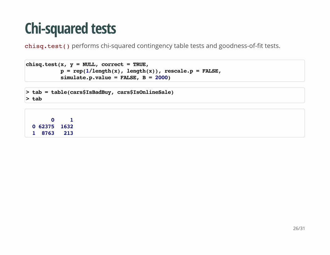
Chi-squared testschisq.test() performs chi-squared contingency table tests and goodness-of-fit tests.

chisq.test(x, y = NULL, correct = TRUE, p = rep(1/length(x), length(x)), rescale.p = FALSE, simulate.p.value = FALSE, B = 2000)

> tab = table(cars$IsBadBuy, cars$IsOnlineSale)> tab

0 1 0 62375 1632 1 8763 213

26/31

Chi-squared testsYou can also pass in a table object (such as tab here)

> cq=chisq.test(tab)> cq

Pearson's Chi-squared test with Yates' continuity correction

data: tabX-squared = 0.9274, df = 1, p-value = 0.3356

> names(cq)

[1] "statistic" "parameter" "p.value" "method" "data.name" "observed" [7] "expected" "residuals" "stdres"

> cq$p.value

[1] 0.3356

27/31

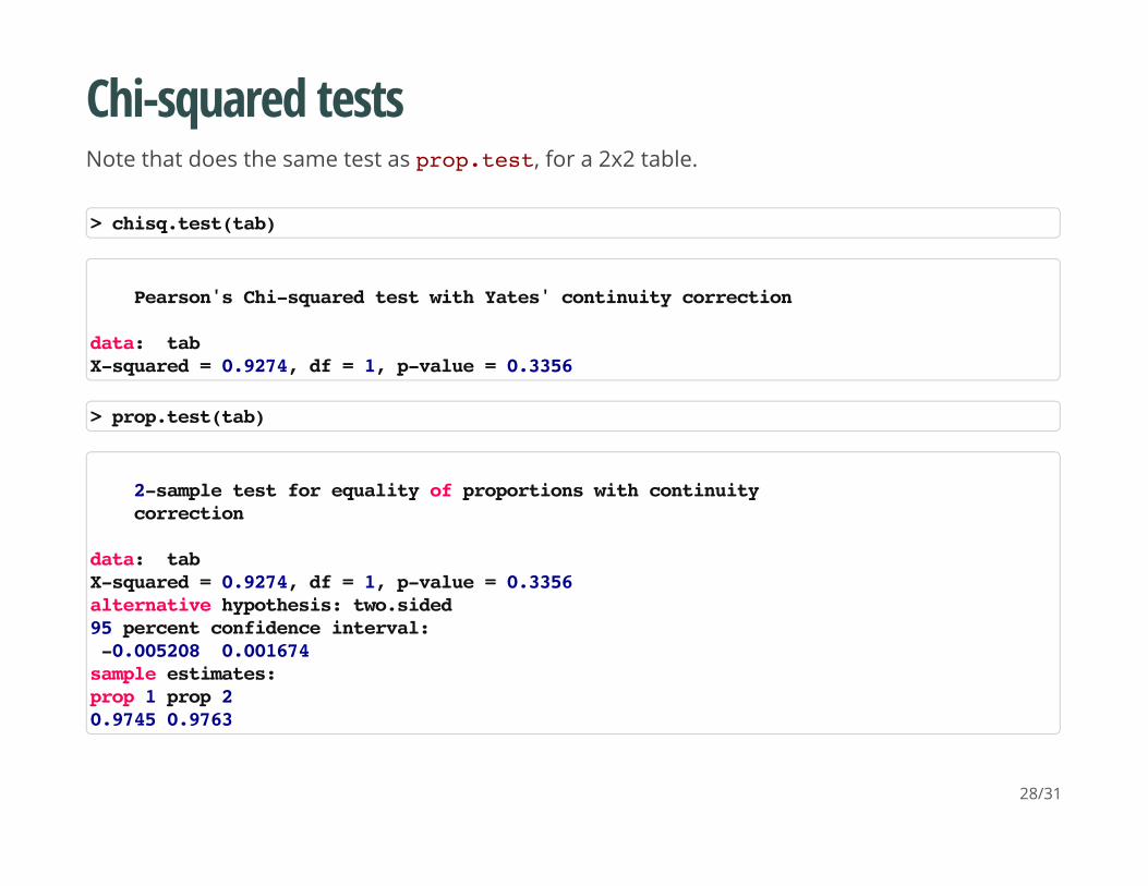
Chi-squared testsNote that does the same test as prop.test, for a 2x2 table.

> chisq.test(tab)

Pearson's Chi-squared test with Yates' continuity correction

data: tabX-squared = 0.9274, df = 1, p-value = 0.3356

> prop.test(tab)

2-sample test for equality of proportions with continuity correction

data: tabX-squared = 0.9274, df = 1, p-value = 0.3356alternative hypothesis: two.sided95 percent confidence interval: -0.005208 0.001674sample estimates:prop 1 prop 2 0.9745 0.9763

28/31

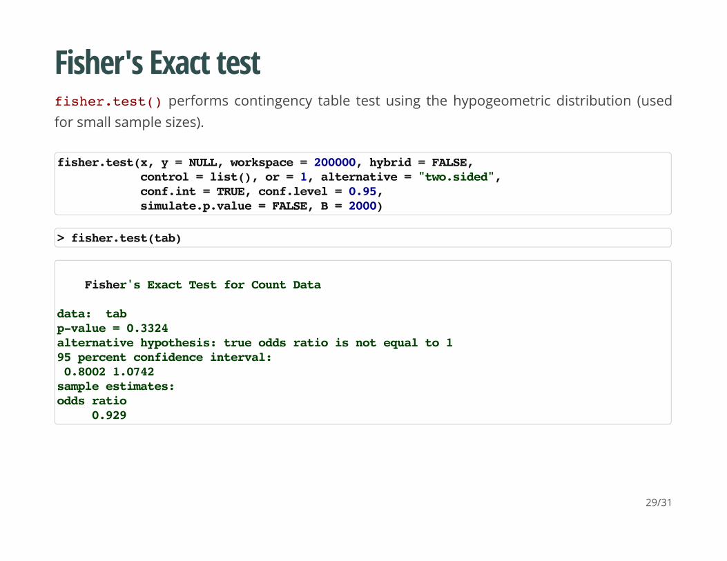
Fisher's Exact testfisher.test() performs contingency table test using the hypogeometric distribution (usedfor small sample sizes).

fisher.test(x, y = NULL, workspace = 200000, hybrid = FALSE, control = list(), or = 1, alternative = "two.sided", conf.int = TRUE, conf.level = 0.95, simulate.p.value = FALSE, B = 2000)

> fisher.test(tab)

Fisher's Exact Test for Count Data

data: tabp-value = 0.3324alternative hypothesis: true odds ratio is not equal to 195 percent confidence interval: 0.8002 1.0742sample estimates:odds ratio 0.929

29/31

Probability DistributionsSometimes you want to generate data from a distribution (such as normal), or want to seewhere a value falls in a known distribution. R has these distibutions built in:

Normal

Binomial

Beta

Exponential

Gamma

Hypergeometric

etc

·

·

·

·

·

·

·

30/31

Probability DistributionsEach has 4 options:

r for random number generation [e.g. rnorm()]

d for density [e.g. dnorm()]

p for probability [e.g. pnorm()]

q for quantile [e.g. qnorm()]

·

·

·

·

> rnorm(5)

[1] 1.8969 0.1496 1.6520 -0.6859 0.3021

31/31