Module 3: Quality and timecga-education.org/2009-10/ma2/module03.pdf · 2009-02-23 · You learn...

Module 3: Quality and time

Overview

Module 3 examines the relationship between cost, quality, and time, and explains how quality and time can be used as strategic competitiveness tools. It introduces the cost-of-quality report, and links it with benchmarking to outline the relationship between quality and corporate strategy. You learn about the theory of constraints, and conclude the module by analyzing and solving a cost-of-quality business case.

Test your knowledge

Begin work on this module with a set of test-your-knowledge questions designed to help you gauge the depth of study required.

Learning objectives

3.1 Explain how quality is used as a competitiveness tool. (Level 2)

3.2 Evaluate a cost-of-quality program by calculating categories of cost and analyzing nonfinancial measures. (Level 1)

3.3 Outline the three methods companies use to identify internal quality problems. (Level 1)

3.4 Analyze relevant costs and benefits of quality improvements. (Level 1)

3.5 Explain how managers use information about costs of design quality. (Level 2)

3.6 Evaluate quality performance using financial and nonfinancial measures. (Level 1)

3.7

Explain the impact of time on quality and competitiveness. (Level 2)

3.8 Analyze relevant revenues and costs of time. (Level 1)

3.9 Explain how to maximize throughput contribution using the theory of constraints. (Level 1)

3.10 Analyze a cost-of-quality scenario, and make a recommendation. (Level 1)

MA2 - Module 3 Page 1

http://lms.cga-canada.org/includedmedia/2008-09/MA2/MA2_TYK/m03/flash_quiz_client.html

3.1 Quality as a competitiveness tool

Learning objective

● Explain how quality is used as a competitiveness tool. (Level 2)

Required reading

● Chapter 19, pages 738-740

LEVEL 2

Focusing on quality has long been a strategy that companies use to gain competitive advantage. Companies worldwide are turning management attention to the concept of quality, and international standards (for example, ISO 9001) have recently emerged to mandate quality levels.

Quality improvements can lead to reduced costs — through less waste, spoilage, and rework — and result in higher levels of customer satisfaction. Global concern for the environment and effects of climate change are also creating a greater need for companies to focus on quality initiatives that reduce waste; the quality of a good or service is driven by consumer demand, and today’s consumers are demanding that goods or services be produced without further damage to the environment.

The term quality refers to many factors, including degrees of fitness for use, levels of customer satisfaction, and degree of meeting design and engineering specifications. Here are the two important, and interrelated, aspects of quality:

● Design quality measures how closely the product characteristics or services performed meet the needs and wants of consumers.

● Conformance quality measures performance of a product or service according to design and production specifications.

Page 740 of the text shows a diagram of the relationship between design quality and conformance quality.


3.2 Costs of quality

Learning objective

● Evaluate a cost-of-quality program by calculating categories of cost and analyzing nonfinancial measures. (Level 1)

Required reading

● Chapter 19, pages 740-743 (to "The Internal Business-Process Perspective: Analyzing and Improving Quality")

LEVEL 1

The following four costs of quality (COQ) are incurred to prevent or correct conditions and/or processes that result in low-quality products:

● Prevention costs are incurred to prevent production of products that do not conform to specifications (including engineering design costs).

● Appraisal costs are incurred to detect products or services that do not conform to specifications (including all inspection of products).

● Internal failure costs are incurred to detect nonconforming products before they are shipped to customers (including rework, spoilage, and scrap costs).

● External failure costs are incurred to detect a nonconforming product after it is shipped (including costs of lost reputation, rework/warranty, and customer support).

Generally, costs for prevention should reduce the costs of the other three areas. Exhibit 19-1 on page 741 provides a list of typical costs in each category and Exhibit 19-2 on page 742 provides a detailed analysis of activity-based costs of quality, including an opportunity cost analysis for lost external failure costs (panel B).

Nonfinancial measures of quality

For success in the marketplace, a product must meet customer demand. Measures related to the Balanced Scorecard customer perspective allow management to see how well the cost of quality goal is being met. When customers are unhappy because of poor quality, this is reflected in such measures as market share, defect rates, and customer complaints. Measures of customer quality and time are reflected in on-time delivery rates, customer service response times, and customer survey responses.


3.3 Analyzing and improving quality

Learning objective

● Outline the three methods companies use to identify internal quality problems. (Level 1)

Required reading


LEVEL 1

To identify internal quality problems, companies analyze internal business processes using the following three methods:

●

Statistical quality control (SQC), or statistical process control (SPC) — Statistically maps the random or nonrandom variations in the operating process. A control chart representing a particular step, operation or procedure over time is often used to accomplish this. Exhibit 19-3 on page 744 shows SQC charting using arithmetic average and standard deviations. According to the 2-sigma rule, a point that falls out of the 2-sigma would occur in a normal distribution only 5% of the time and should be investigated.

●

Pareto diagram — Observations outside of set limits or frequencies show how frequently each type of defect occurs, and help management identify any major problems (Exhibit 19-4).

●

Cause-and-effect diagram — The most frequently occurring problems in the Pareto diagram are analyzed through a cause-and-effect diagram (also known as a fishbone diagram). Each cause factor is represented by an additional arrow on the diagram (Exhibit 19-5).


3.4 Costs and benefits of quality improvement

Learning objective

●

Analyze the relevant costs and benefits of quality improvements. (Level 1)

Required reading


LEVEL 1

After internal business processes have been analyzed, changes are suggested to fix any problems identified. An analysis of relevant costs and benefits must then be performed for each suggested alternative. Relevant costs and benefits are those that change between alternatives, and can take the form of increased (or decreased) costs or additional (or reduced) revenues.

Exhibit 19-6 on page 746 shows a comparative analysis of the estimated effects of proposed alternatives in the example. Managers make strategic choices based on the results of the analysis; these choices then require a further sensitivity analysis. Managers consider the following effects of nonfinancial information and underlying economic conditions, which may change levels of sales and production costs.

● Opportunity costs — For example, when space used to achieve one option can be used for an alternative production process, managers determine the lost contribution margin on the alternative process.

● The COQ report — Determines the impact of interdependencies across the four categories of quality-related costs; for example, redesigning the production process can increase prevention costs but cause a reduction in internal and external failure costs.

● Trends of quality costs over time — For example, a company may look at the percentage of sales that each category represents over a number of periods to see the overall impact of proposed changes, since many alternatives will have multi-period effects.

The Firestone case on pages 747-748 provides an even stronger message about the costs of failure to make quality improvements. In analyzing the situation, the managers failed to take into account all stakeholders. The most important negative effect for the company was the perceived lack of concern for the safety of its customers and the very real potential for serious harm to those customers, which should have been the primary factor in dealing with the situation. This is a clear case where the company should have immediately made safety quality improvements or withdrawn the product from the market.


3.5 Costs of design quality

Learning objective

●

Explain how managers use information about the costs of design quality. (Level 2)

Required reading

● Chapter 19, pages 748-749 (to "Evaluating Quality Performance")

LEVEL 2

Companies must also focus on costs of design quality. Poorly designed processes — production, marketing, distribution, and customer service — result in lost opportunity costs. Because of the difficulty in assigning costs to these areas, (see page 748), most companies don’t measure the financial costs of design quality. However, these costs are reflected to some extent in nonfinancial measures (that is, mostly in the internal-business process area). Prevention, appraisal, and internal failure costs also have nonfinancial measures, including defect rates, rework percentages, and number of design changes.

The COQ report and the Balanced Scorecard are planning and control mechanisms that management accountants use to measure the success of a corporation’s strategy. Measuring changes over time and analyzing the changes using a variety of perspectives helps managers gain a better understanding of the cost connections between the four areas of COQ reports and their effects on the organization’s overall strategy. The learning and growth perspective of the Balanced Scorecard (which includes such measures as employee turnover and satisfaction ratios, employee training, and research and design ratios to proposed output) also links to the COQ report and provides managers with information on the connections and trends that affect quality and costs. Efforts at improvement focused on the learning and growth perspective should show up in the trends in the COQ report.


3.6 Evaluating quality performance

Learning objective

●

Evaluate quality performance using financial and nonfinancial measures. (Level 1)

Required reading


LEVEL 1

Quality is critical to the success of a company, whether it is a service organization or a manufacturing business. Managers assess the company’s input, processes, and output to determine its competitive position. The COQ report helps managers gauge the company’s quality initiatives. To understand COQ reports, both financial and nonfinancial aspects of quality should be analyzed together. The following case shows how quality reporting works to isolate as many quality factors as possible to allow managers to effectively address quality problems.

Example 3.6-1: Cost-of-quality report at Mastiff Appliances

Mastiff Appliances Inc. builds small household appliances such as irons, coffee makers, battery-powered screwdrivers, and similar items. For a long time, Mastiff held a reputation for strong, durable, and reliable appliances. This reputation began to decline, however, when increased competition forced the company to cut costs and this was handled poorly. For a moderate period following the cost cutting, as long as the company was able to take advantage of its reputation, Mastiff’s sales remained relatively steady. This effect then all but disappeared. The loss of reputation, coupled with increased overseas competition, caused Mastiff’s sales to plummet sharply.

On January 1, 20X6, Mastiff began a massive effort directed toward quality control. In the two years that followed, sales failed to go up but remained steady at around $10 million per year. A significant amount of money was spent on testing equipment, increasing inspection, setting up a statistical process control system, and reworking or throwing out defective items. Upper management began to wonder if the company was spending and using resources effectively.

Costs over the last three years related to quality and quality control are listed in Exhibit 3.61.

Exhibit 3.6-1: Mastiff Appliances — Quality and control costs

20X5 20X6 20X7Amortization of testing equipment $ 22,000 $ 34,000 $ 30,000

Disposal of defective products 54,000 76,000 60,000

Inspection 76,000 120,000 132,000Net cost of scrap 86,000 124,000 100,000Product recalls 340,000 82,000 40,000Product testing 98,000 160,000 170,000Quality engineering 56,000 80,000 84,000Rework labour 140,000 200,000 180,000Statistical process control — 74,000 78,000Supplies used in testing 4,000 6,000 7,000Systems development 64,000 106,000 117,000Warranty repairs 420,000 140,000 70,000Warranty replacements 60,000 18,000 5,000Total $1,420,000 $1,220,000 $1,073,000


Is Mastiff focusing its quality initiatives in the right areas? Were managers making the right quality decisions? In answering this question, a COQ report would provide managers with useful information. A trend analysis of nonfinancial quality information would also give management a better idea of how well the quality problem has been handled.

Preparing a COQ report

Step 1: Determine direct and indirect quality costs

Because this is an illustration rather than an actual business, the quality costs are given. In the real world, determining which direct and indirect costs are quality costs is a significant part of the exercise. If scrap costs are viewed not simply as a cost of manufacture but as a cost of quality, which could be reduced by changes in behaviour, then a significant change in approach could result.

Step 2: Categorize quality costs

Once the direct and indirect costs of quality are defined and determined, the costs are sorted into the four categories: prevention, appraisal, internal failure, and external failure. This provides strong evidence that spending in the prevention stage can lead to significant cost savings at later stages. It is most useful to present these quality costs in terms of a sales percentage so that the impact of quality cost on the profitability of the company is linked and apparent. The quality-cost report for Mastiff Appliances follows in Exhibit 3.6-2.

Exhibit 3.6-2: Mastiff Appliances — COQ report

Mastiff’s effort at quality control (Exhibit 3.6-3) shifted the timing and amount of money the company spent on quality. Prevention costs went from $120,000 in 20X5 to $279,000 in 20X7. Likewise, appraisal costs moved from $200,000 to $339,000. This increased spending on prevention and appraisal more than paid off with reductions in both internal and external failures as follows:

● Total expenditures on quality decreased from $1,420,000 to $1,073,000 over three years, or from 14.2% of sales to 10.73%.

●

External failure costs dropped from a total of $820,000 to $115,000.

Exhibit 3.6-3: Mastiff Appliances — Quality costs for the years ended 20X5, 20X6, and 20X7


Evidence from both sales and the COQ report support the decision taken by management to focus on quality.

Total expenditures on quality dropped by $200,000 in 20X6 and by $347,000 in 20X7. External failure costs dropped from 8.2% of sales in 20X5 to 1.15% of sales in 20X7. Given that external failures are those captured by the customer, this percentage has a direct effect on product reputation.

That sales remained relatively stable for two years indicates that the emphasis on quality to the customer is


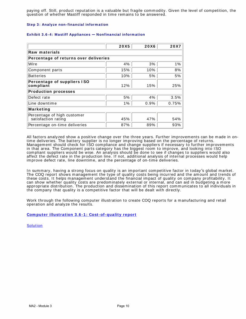
paying off. Still, product reputation is a valuable but fragile commodity. Given the level of competition, the question of whether Mastiff responded in time remains to be answered.

Step 3: Analyze non-financial information

Exhibit 3.6-4: Mastiff Appliances — Nonfinancial information

20X5 20X6 20X7

Raw materials

Percentage of returns over deliveries

Wire 4% 3% 1%

Component parts 15% 10% 8%

Batteries 10% 5% 5%

Percentage of suppliers ISO compliant 12% 15% 25%

Production processes

Defect rate 5% 4% 3.5%

Line downtime 1% 0.9% 0.75%

Marketing

Percentage of high customer satisfaction rating 45% 47% 54%

Percentage on-time deliveries 87% 89% 93%

All factors analyzed show a positive change over the three years. Further improvements can be made in on-time deliveries. The battery supplier is no longer improving based on the percentage of returns. Management should check for ISO compliance and change suppliers if necessary to further improvements in that area. The Component parts category has the biggest room to improve, and looking into ISO compliant suppliers would be wise. An analysis should be done to see if changes to suppliers would also affect the defect rate in the production line. If not, additional analysis of internal processes would help improve defect rate, line downtime, and the percentage of on-time deliveries.

In summary, having a strong focus on quality is an important competitive factor in today’s global market. The COQ report shows management the type of quality costs being incurred and the amount and trends of these costs. It helps management understand the financial impact of quality on company profitability. It can show whether quality costs are predominately external or internal, and can aid in budgeting a more appropriate distribution. The production and dissemination of this report communicates to all individuals in the company that quality is a competitive factor that will be dealt with directly.

Work through the following computer illustration to create COQ reports for a manufacturing and retail operation and analyze the results.

Computer illustration 3.6-1: Cost-of-quality report

Solution


Computer illustration 3.6-1: Cost-of-quality report

Deresh Soccer Equipment Ltd. manufactures and sells soccer equipment through its own retail outlets. In the last four years the company has been focusing on improving quality performance.

Exhibit 3.6-5: Deresh Soccer — Financial information pertaining to quality for 20X4, 20X5, 20x6, and 20X7 (in thousands).

Material provided

● File MA2M3P1 containing a partially completed worksheet M3P1 and the solution worksheet M3P1S

Required

Using the information given in Exhibit 3.6-5, create a COQ report for Deresh Soccer. Analyze the trends seen in the cost of quality report. Has Deresh’s focus on quality yielded any results? Procedure

1. Start Excel.


2. Open the file MA2M3P1. Go to TAB M3P1.

3. Review the spreadsheet. Note that the data table replicates the information given

above. Also note that cells A28 to K65 contain the format for a cost-of-quality report.

4. In Column A enter the titles for the cost types based on the information in the data table. Use a formula for this.

5. Complete the cost of quality report by entering formulas in cells D37 to K40; D45 to K48; D53 to K55 and D59 to K62. Note that cells in columns E, G, I, and K should not reference the data table. These cells calculate the percentage of total sales for the year represented by the cost-of-quality item on that row.

6. In rows 41, 49, 56, and 63 enter a formula to calculate the total of each type of cost for each year and the total percentage.

7. In cell D65 enter an IF formula that verifies that all costs of quality from the data table have been included in the report. Use a similar formula for cells F65, H65, and J65.

8. In cells E65, G65, I65, and K65 enter an IF formula that verifies the total percentages.

9. Now click the M3P1S tab to verify that you have correctly created the Cost-of-Quality Report for Deresh Soccer Equipment.


Computer illustration 3.6-1 Solution

It is evident from the trends in the cost-of-quality report that Deresh Soccer Equipment has focused its attention on prevention costs. The increase in prevention costs has been more than offset by the savings in external failure costs. Total quality costs have been reduced by about 2%. While appraisal costs are up, internal failure costs are down. The company may want to focus on specific preventative items that will help keep the appraisal costs down. Some analysis of nonfinancial performance measures might help improve the materials procurement and product testing processes.


3.7 Time and competitiveness

Learning objective

● Explain the impact of time on quality and how time can be used for competitive advantage. (Level 2)

Required reading


LEVEL 2

Time is a critical quality variable in the success of many organizations. Fast food restaurants, furniture movers, couriers, and airlines — like McDonalds, United Van Lines, Purolator, and Air Canada — all use detailed measures of time to determine the success of their products or services. Customer response time and on-time performance are two commonly used measures of time as a quality variable:

● Customer response time is the time interval from customer order to product or service delivery. Exhibit 19-7 on page 751 identifies components of customer-response time. Manufacturing-lead (or cycle) time is the interval from when an order is ready to start (or be setup) on the production line to completion (finished good). Order-delivery time is the interval from finished good to delivery to the customer.

●

On-time performance is usually expressed as a percentage representing the ratio of times a product or service is delivered according to schedule to all deliveries. For example, Air Canada would report times that planes arrived at destinations at the scheduled times as a percentage of total flights.

Speed to market has become a key determinant in competitive success for many industries, especially high-tech firms. Being the first to market with new products is a key strategy for many companies, as it provides a high return and early patent protection allows companies to earn a premium on first-to-market products.

Responding efficiently to customers’ needs can make a firm’s reputation, and failure to respond quickly can send customers to the competition. Knowing customers’ needs with respect to time is important in knowing how to capitalize on time as a competitiveness tool. For example, an airline passenger informed that a flight will take 4 hours and 25 minutes but who is then delayed, even for a short while, will be disappointed. An airline that earns a reputation for delayed flights will lose customers to the competition.


3.8 Time drivers and costs of time

Learning objective

● Analyze relevant revenues and costs of time. (Level 1)

Required reading


LEVEL 1

A time driver is any factor that causes a change in the speed with which an activity is accomplished (for example, uncertainty about when a client or customer will place an order, limited capacity leading to bottlenecks in production, and so on). Companies often address these factors through plant layout, product design, and production scheduling.

An important factor in production scheduling is the average wait time needed for production, which can be computed as follows:

For example, Baker receives 200 orders per year, average manufacturing time is 10 hours, and the machine has a capacity of 20,000 hours per year.

Relevant revenues and costs of time

Companies must consider that time affects both revenue and costs. Customers will often pay a higher price for faster delivery or service, while carrying costs (such as inventory, rent, spoilage, waste, deterioration) are increased for slower production times. When capacity is limited, opportunity costs become more important. Introduction of a new product or service may have a negative impact on existing products. Companies planning to introduce new versions of a product must consider whether to continue to carry the old product, and must also be aware that cannibalization (that is, a new product having a negative effect on sales of an existing product by splitting the market or changing production parameters) could occur.

Exhibit 19-8 (page 755) considers the possible negative effects of introducing a new product to the existing line of products. In that situation, the average wait time for the current product increased substantially, which affected the company’s ability to fulfill demand for the product. Such a bottleneck could be alleviated with the purchase of a new machine (which then becomes a capital budgeting issue).


3.9 Theory of constraints

Learning objective

● Explain how to maximize throughput contribution using the theory of constraints. (Level 1)

Required reading


LEVEL 1

The theory of constraints describes methods that can be used to maximize operating income in the face of bottlenecks or constraints. The following three measurements are important to the theory:

●

Throughput contribution — Sales revenue minus direct material costs. Throughput is the rate at which an organization generates cash from the sale of products. Throughput costing defines variable direct material as the only cost included in inventory. Throughput contribution then could be considered as the net rate at which cash is generated from the sale of products. In your introductory management accounting course, you studied absorption and variable costing, where the principle difference in inventory valuation is the inclusion of fixed manufacturing overhead in absorption costing. Throughput costing is a third inventory valuation technique that considers only direct material as relevant to inventory valuation (product cost) and considers that conversion costs (direct labour and manufacturing overhead) are period costs, charged in the period in which they are incurred.

●

Investments (inventory) — Sum of direct material, work in process and finished goods inventory, R&D costs, and the cost of equipment and buildings.

●

Operating costs — Sum of all operating costs, other than direct materials, incurred to earn throughput contribution (includes wages and salaries, rent, utilities, property taxes, amortization).

The objective is to increase throughput contribution while simultaneously decreasing investment in inventory and operating costs. The method assumes that the situation under consideration is short-term and that other current operating costs are fixed. Short-term consideration means that the focus is on the immediate improvement of a specific constraint that is currently slowing throughput. This also reinforces the assumption that all other costs are fixed; in the short-term, most costs are considered fixed.


Steps in managing bottlenecks

1. Recognize that the bottleneck is related to throughput contribution as a whole. A firm can only produce the number of products that its slowest process can produce.

2. Search and find the bottleneck resource by identifying the process where large quantities of resources are waiting for production.

3. Keep the bottleneck operation busy and subordinate all non-bottleneck resources to the bottleneck resource. This affects the overall production schedule. In relevant costing, you learned that to maximize overall contribution, when scarce resources or constraints exist, you must maximize the contribution per scarce resource.

4. Take action such as the following to increase bottleneck efficiency and capacity:

●

Eliminate idle time (such as production scheduling and plant layout design).

●

Schedule processes to produce products with highest contribution margin per bottleneck.

●

Shift production of bottleneck machine to non-bottleneck machines or consider outsourcing if the item is not strategic.

●

Reduce setup and process time through engineering redesign. ●

Improve quality of production process and parts (poor quality leads to decreased production).

In the long-run, costs that are assumed to be fixed under the theory of constraints must be considered variable costs and analyzed using activity-based costing methods. Activity-based costing focuses on the long-run perspective and on eliminating non-value added products and processes; this approach complements the short-term focus of the theory of constraints.

Outsourcing can also help to alleviate bottlenecks. Analyses of relevant costing, quality, and capital budgeting data can be used to determine whether outsourcing is a viable option. If quality can be maintained, contribution margin increases and potential fixed costs can be reduced over time, which involves capital budgeting analysis and analysis of the time value of money. It is important to note that only non-strategic products and processes should be considered for outsourcing. Competitive advantages, which lead to superior returns, arise from a company’s ability to maximize its core competencies (what it does better than its competitors). Core competencies should be guarded and defended rigorously and not be considered for outsourcing.

Balanced Scorecard and time-related measures

The Balanced Scorecard can be used to identify cause-and-effect relationships that reveal how bottlenecks are created, and it also helps managers determine how to alleviate them. For example, improved employee training can lead to improved efficiency and increased production, which can lead to decreased customer response time and increased customer satisfaction, and ultimately lead


to increased revenues and decreased costs.


3.10 Case: Quality and time initiatives *Updated September 10

Learning objective

●

Analyze a cost-of-quality scenario and make a recommendation. (Level 1)

LEVEL 1

Case 3.10-1: Cost of quality at Welsh Manufacturing Ltd.

Jack Hughes, president of Welsh Manufacturing Ltd. completed a meeting with Jerry Brice, manager of purchasing, with the following comment:

“Something’s got to be done about the costs of the A45 product. Overhead costs have been increasing and direct material costs have skyrocketed over the past six months. What have you got to say about it, Jerry?”

Jack was referring to the increase of production costs for the A45 from $4.50 per unit six months ago to the current cost of $6.65 per unit. The margins have been squeezed so that it appears profit targets for the current year will not be met. Jerry outlined what he knew at this point and agreed to look into the matter.

1. The company uses a normal costing system with budgeted material cost of $1.50 per unit, direct labour of $2.00 per unit and manufacturing overhead charged at 50% of direct labour costs.

2. Eight months ago, Jerry’s department decided to use multiple suppliers, so that they would not be exclusively tied to one major supplier. Many of these new suppliers turned out to be resellers, buying materials purchased from various sources and reselling them to Welsh at a markup.

3. The implementation of a Balanced Scorecard a year ago, was considered a success, but some managers are reluctant to agree with the indicators chosen and question the validity of the results. For example, in the past few months customer satisfaction measures have been falling, and customer complaints have been increasing, even though higher production costs have not been passed on to customers. Salespeople are blaming customer’s greed for the current situation. They feel that the customers are demanding too much of the company.

4. Jerry gathered the following additional information on the A45 product line for comparison:

20X7 20X8 (6-months)

Revenues (50,000 / 20,000 units) $490,000 $200,000 Direct material ($1.50 / 1.95) 75,000 39,000 Direct labour ($1.90 / 2.25) 95,000 45,000 Manufacturing overhead applied 47,500 22,500


Manufacturing overhead actual 47,000 49,000 Additional costs: 1,000 3,000 Scrap costs 1,000 3,000 Design engineering 5,000 2,500 Customer complaints 90 134 On-time delivery 96% 91% Warranty liability 8,500 6,200 Product inspection 4,000 4,000 Rework 3,000 8,000

Required

On the basis of the information available, what would be the next steps for Jerry to consider?

Solution


Case 3.10-1: Cost of quality at Welsh Manufacturing Ltd.

Solution

Jerry should consider the reasons for the increased costs as well as the decreased customer satisfaction. Possible suggestions would include preparing a cost of quality analysis as follows:

Cost of quality analysis

It is apparent from the cost of quality analysis that internal and external failures have increased substantially in the past 6 months. By using the percentages, you can factor out that you are looking at only 6 months worth of data for 20X8 against the full year’s data for 20X7. It appears that problems related to product materials may be at issue, since the cost per unit for material has increased, yet rework and scrap costs are up. It would also be useful to do a variance analysis (Module 2) to further back these findings. The use of multiple suppliers, especially resellers, could have had an impact on the level of control of materials, as there seems to be poor quality product inputs. This could directly affect the amount of rework and scrap noticed during the period, as well as the resulting increase in overall cost to produce good units. The overhead costs are approximately double the amount applied in 20X8, which could result from changes in manufacturing design (although this does not appear to be the case). The pre-determined overhead rate may be incorrect and not reflect the current operating environment. Costs related to manufacturing overhead, such as rent or property taxes, could have increased. Inspection costs have doubled compared to the previous year, which could relate to salary increases and the additional work being performed because of the high amount of rework required. Another area of concern for the company is the decrease in customer satisfaction. It should be noted that, although the cost of quality report looks at financial


numbers, a Balanced Scorecard looks at both financial and nonfinancial analyses. The additional information relating to the decline in on-time delivery (possibly due to the rework) or problems in delivery and scheduling should be looked into. Are there problems with manufacturing lead-time? The efficiency and effectiveness of the production line needs to be examined. Further, assuming complaints are even throughout the year, the increase in customer complaints is almost 300% per annum 134 ÷ 90 = 148% x 2 = 296% (148% increase is for the first 6 months only, assumes 268 complaints in 20X8). It appears that salespeople are not in touch with the needs of customers, as they believe customers are over-demanding. Salespeople should conduct focus groups with both satisfied and non-satisfied customers to determine the reasons for dissatisfaction and for the increase in customer complaints.


Module 3 summary *Updated September 10

Explain how quality is used as a competitiveness tool

Quality is a key method for gaining a competitive advantage. Here are the two basic aspects of quality:

● Quality of design — Does the design meet the requirements of the consumers?

● Conformance quality — Does the product meet the design and production specifications?

Evaluate a cost-of-quality program by calculating categories of cost and analyzing nonfinancial measures

The four categories of costs are as follows:

● Prevention● Appraisal● Internal failure● External failure

Outline the three methods companies use to identify internal quality problems

Statistical quality control is used to map random and nonrandom variation in operation processes.

Pareto diagram is used to show frequency of defect by type.

Cause-and-effect diagrams is used to identify the root of problems.

Analyze relevant costs and benefits of quality improvements

Suggested changes based on analysis are analyzed again to determine cost and benefit.

Relevant costs change between alternatives. A sensitivity analysis should be performed.

Opportunity costs should be considered.


Explain how managers use information about costs of design quality

Design quality includes costs of poorly designed products including production, marketing, distribution, and customer-service costs.

Nonfinancial measures may be more useful.

The learning and growth perspective of the Balanced Scorecard links to cost of quality through employee turnover and satisfaction rates.

Evaluate quality performance using financial and nonfinancial measures

Cost-of-quality reports are used to look at trends in quality over time.

Changes between prevention costs and external failure costs show how investing in preventing quality issues substantially reduces external failure costs.

Nonfinancial information should indicate trends to the key Balanced Scorecard perspectives.

Explain the impact of time on quality and competitiveness

Speed to market has become one of the key competitive advantages.

Two common measures are:

● Customer response time — the time between the placing of an order and when the customer receives the product

● On-time performance — percentage of times that product or service was delivered according to or ahead of schedule

Analyze relevant revenues and costs of time

Two major time considerations are uncertainty about when an order will be placed and limited capacity.

Average wait time = [average number of orders x (manufacturing time)2] ÷ (2 x [annual capacity of machine – (average number of orders x manufacturing time)]).

Opportunity costs and product cannibalization need to be assessed.

Explain how to maximize throughput contribution using the theory


of constraints

The three key measurements are:

● Throughput contribution● Investments● Operating costs

Steps in managing bottlenecks are:

1. Recognize bottleneck relation to throughput contribution.2. Find the bottlenecked resource.3. Keep the bottleneck operation busy and subordinate other processes to it.4. Increase the bottleneck efficiency and capacity.

Analyze a cost-of-quality scenario and make a recommendation

Note: There is no text after “Analyze a cost-of-quality scenario and make a recommendation.” The topic is a case study and students are advised to read all case studies carefully.


Module 3 self-test

Question 1

Exercise 19-16, pages 761-762 Solution

Question 2

Exercise 19-18, page 763 Solution

Question 3

Exercise 19-23, pages 765-766 Solution

Note:

●

In part 2 on page 766, the last sentence states that the goal is for the bank to be able to achieve an average wait time of 4.5 minutes or less. Based on the information given, this is an error; the average wait time that the bank wants to achieve is 5 minutes or less, not 4.5 minutes.

●

In part 3, the last sentence mentions an average wait time of 4.5 minutes. The 4.5 minutes is the customer service time, not the wait time, which should be 5 minutes.

Question 4

Exercise 19-24, page 766 Solution

Question 5

Problem 19-31, page 769 Solution

Question 6

Problem 19-32, page 769 Solution


Self-test 3

Solution 1

1. The ratio of each COQ category to revenues for each period is as follows:

Semi-annual Costs of Quality Report Bergen, Inc. (in thousands)

6/30/2007 12/31/2007 6/30/2008 12/31/2008 % of Rev. % of Rev. % of Rev. % of Rev. (2) = (4) = (6) = (8) = (1) (1)÷4,944 (3) (3)÷5,448 (5) (5)÷5,580 (7) (7)÷5,412 Prevention costs Machine maintenance$ 258 $ 258 $ 228 $ 192 Training suppliers 6 54 24 18 Design reviews 24 122 120 114 288 5.8% 434 8.0% 372 6.7% 324 6.0% Appraisal costs Incoming inspection 54 64 43 26 Final testing 192 192 168 113 246 5.0% 256 4.7% 211 3.8% 139 2.6% Internal failure costs Rework 144 127 106 74 Scrap 82 77 50 48 226 4.6% 204 3.7% 156 2.8% 122 2.2% External failure costs Warranty repairs 83 37 30 28 Customer returns 314 301 139 96 397 8.0% 338 6.2% 169 3.0% 124 2.3% Total quality costs $1,157 23.4% $1,232 22.6% $ 908 16.3% $ 709 13.1% Total production and revenues $4,944 $5,448 $5,580 $5,412

From an analysis of the Cost of Quality Report, it would appear that Bergen Inc.’s program has been successful since • Total quality costs as a percentage of total revenues have declined from 23.4%

to 13.1%. • External failure costs, those costs signaling customer dissatisfaction have

declined from 8% of total revenues to 2.3%. These declines in warranty repairs and customer returns should translate into increased revenues in the future.

• Internal failure costs have been reduced from 4.6% to 2.2% of revenues. • Appraisal costs have decreased from 5.0% to 2.6%. Preventing defects from

occurring in the first place is reducing the demand for final testing. • Quality costs have shifted to the area of prevention where problems are solved

before production starts. Maintenance, training, and design reviews have increased from 5.8% of total revenues to 6% and from 24.9% of total quality costs ($288 ÷ $1,157) to 45.7% ($324 ÷ $709). The $36,000 increase in these costs is more than offset by decreases in other quality costs.


Because of improved designs, quality training, and additional pre-production inspections, scrap and rework costs have declined. Production does not have to spend an inordinate amount of time with customer service since they are now making the product right the first time and warranty repairs and customer returns have decreased.

2. To measure the opportunity cost of not implementing the quality program, Bergen

Inc. could assume that

• Sales and market share would continue to decline if the quality program had not been implemented and then calculate the loss in revenue and contribution margin.

• The company would have to compete on price rather than quality and calculate the impact of having to lower product prices.

Opportunity costs are not recorded in accounting systems because they represent the results of what might have happened if Bergen had not improved quality. Nevertheless, opportunity costs of poor quality can be significant. It is important for Bergen to take these costs into account when making decisions about quality.


Self-test 3

Solution 2

1. and 2. Sales, Costs of Quality and Costs of Quality

as a Percentage of Sales for Olivia Sales = $2,400 × 10,000 units = $24,000,000 Percentage of Sales Cost (2) = (1) ÷ Costs of Quality (1) $24,000,000

Prevention costs Design engineering ($90 × 6,000 hours) $ 540,000 2.25% Appraisal costs Question 2 cont’d Testing and inspection ($48 × 1 hour × 10,000 units) 480,000 2.00% Internal failure costs Rework ($600 × 5% × 10,000 units) 300,000 1.25% External failure costs Repair ($720 × 4% × 10,000 units) 288,000 1.20% Total costs of quality $1,608,000 6.70%


Sales, Costs of Quality and Costs of Quality as a Percentage of Sales for Solta

Sales: $1,800 × 5,000 units = $9,000,000 Percentage of Sales Cost (2) = (1) ÷ Costs of Quality (1) $9,000,000

Prevention costs Design engineering ($90 × 1,000 hours) $ 90,000 1.00% Appraisal costs Testing and inspection ($48 × 0.5 × 5,000 units) 120,000 1.33% Internal failure costs Rework ($480 × 10% × 5,000 units) 240,000 2.67% External failure costs Repair ($540 × 8% × 5,000 units) 216,000 2.40% Estimated forgone contribution margin on lost sales [($1,800 – $960) × 300] 252,000 2.80% Total external failure costs 468,000 5.20% Total costs of quality $918,000 10.20% Costs of quality as a percentage of sales are significantly different for Solta (10.20%) as compared with Olivia (6.70%). Ontario spends very little on prevention and appraisal activities for Solta, and incurs high costs of internal and external failures. Ontario follows a different strategy with respect to Olivia, spending a greater percentage of sales on prevention and appraisal activities. The result: fewer internal and external failure costs and lower overall costs of quality as a percentage of sales than with Solta. 3. Examples of nonfinancial quality measures that Ontario Industries could monitor

as part of a total-quality-control effort are (a) Outgoing quality yield for each product. (b) Returned refrigerator percentage for each product. (c) On-time delivery. (d) Employee turnover.


Self-test 3

Solution 3

1. If the branch expects to receive 60 customers each day and it takes 4.5 minutes

to serve a customer, the average time that a customer will wait in line before being served is:

( )( )

( )( )

260 4.5 60 20.25 60 20.25 1, 215 20.25 minutes2 300 270 2 30 602 300 60 4.5

⎡ ⎤× × ×⎣ ⎦= = = = =× − ×× − ×⎡ ⎤⎣ ⎦

2. Suppose the bank counter is kept open for X minutes. Then we want

( )( )

260 4.5 5 minutes2 X 60 4.5

⎡ ⎤×⎣ ⎦= =× − ×⎡ ⎤⎣ ⎦

that is, 60 × 20.25 = 10(X – 270) X – 270 = (60 × 20.25) ÷ 10 = 121.5 X = 391.5 minutes

The counter must be kept open for 391.5 minutes to reduce average waiting time to 5 minutes.1

3. Incremental operating income from providing new services $36 Incremental teller cost (2 additional hours × $12 per hour)2 24 Net increase in operating income from providing new services $12

Yes, the bank should offer the new services since the relevant benefits exceed the relevant costs.3

1) The assumption here is that the customer rate (# of customers per hour) is constant. 2) 91.5 minutes or a little over 1.5 hours of teller time have to be added. Since tellers are paid in increments of an hour, this means 2 additional hours of incremental teller cost. 3) The assumption here is that only variable labour costs matter. However, if variable

and/or fixed overhead costs changed upwards as a result of the extra 1.5 hours of operating time, gross margin analysis would be required.


Self-test 3

Solution 4

1. Finishing is a bottleneck operation. Hence, producing 1,000 more units will

generate additional throughput contribution and operating income.

Increase in throughput contribution ($86.40 – $38.40) × 1,000 $48,000 Incremental costs of the jigs and tools 36,000 Net benefit of investing in jigs and tools $12,000

Mayfield should invest in the modern jigs and tools because the benefit of higher throughput contribution of $48,000 exceeds the cost of $36,000.

2. The Machining Department has excess capacity and is not a bottleneck operation.

Increasing its capacity further will not increase throughput contribution. There is therefore no benefit from spending $6,000 to increase the Machining Department’s capacity by 10,000 units. Mayfield should not implement the change to do setups faster.


Self-test 3

Solution 5

1. SRG expects to use 4,800 (96 hours per order × 50 orders) hours of total capacity

of 6,000 hours equal to 4,800 80%.6,000

=

2. Average manufacturing lead time for Z39

Average waiting time = (average number of orders of Z39 x (manufacturing time for Z39)2) ÷ 2 x [annual machine capacity – (average number of orders of Z39 x manufacturing time for Z39)]

= ( )

( )( ) ( )

250 96 50 9, 216 460,800 192 hours2 6,000 4,800 2 1,2002 6,000 50 96

⎡ ⎤× ×⎣ ⎦ = = =× − ×× − ×⎡ ⎤⎣ ⎦

Average order waitingAverage manufacturing Order manufacturing

time for Z39lead time for Z39 time for Z39

192 hours + 96 hours = 288 hours (12 days)

= +

=

3. Average waiting time for Z39 and Y28

= {[(average number of orders of Z39) x (manufacturing time for Z39)2] + [(average number of orders of Y28) x (manufacturing time for Y29)2]} ÷{2 x [annual machine capacity – [(average number of orders of Z39) x (manufacturing time for Z39)] –[(average number of orders of Y28) x (manufacturing time for Y28)]}

( ) ( )( ) ( )

( ) ( )[ ]

( )2 250 96 25 24 50 9, 216 25 576 460,800 14, 400

2 6,000 4,800 600 2 6002 6,000 50 96 25 24

475, 200 396 hours1, 200

⎡ ⎤ ⎡ ⎤× + × × + ×⎡ ⎤ +⎣ ⎦ ⎣ ⎦ ⎣ ⎦= = =× − − ×× − × − ×⎡ ⎤⎣ ⎦

= =


timelead time for Z39 time for Z39

396 hours + 96 hours = 492 hours (20.5 days)

= +

=



timelead time for Y28 time for Y28


= +

=

4. Average waiting time 396 94%

Average throughput time for Y28 420= =

Part Y28 spends 94% of the time in the plant, on average, just waiting to be processed!

5. Delays occur in the processing of Z39 and Y28 because (1) uncertainty about how

many orders SRG will actually receive (SRG expects to receive 50 orders of Z39 and 25 orders of Y28) and (2) uncertainty about the actual dates when SRG will receive the orders. The uncertainty (randomness) about the quantity and timing of customer orders means that SRG may receive customer orders while another order is still being processed. Orders received while the machine is actually processing another order must wait in queue for the machine to be free. As average capacity utilization of the machine increases, there is less slack and a greater chance that a machine will be busy when another order arrives.


Self-test 3

Solution 6

1. The direct approach is to look at incremental revenues and incremental costs. Average selling price per order for Y28, which has average operating throughput time of 420 hours $ 9,600 Variable costs per order 6,000 Additional contribution per order from Y28 3,600 Multiply by expected number of orders × 25 Increase in expected contribution from Y28 $90,000

Expected loss in revenues and increase in costs from introducing Y28

Product

(1)

Expected Loss in Revenues from

Increasing Average Manufacturing Lead

Times for All Products

(2)

Expected Increase in Carrying Costs from Increasing

Average Manufacturing

Lead Times for All Products

(3)

Expected Loss in Revenues Plus

Expected Increases in

Costs of Introducing

Y28 (4) = (2) + (3)

Z39 Y28 Total

$30,000a — .

$30,000

$ 7,650b 2,625c $10,275

$37,650 2,625 $40,275

a50 orders × ($32,400 – $31,800) b(492 hours – 288 hours) × $0.75 × 50 orders c(420 hours – 0) × $0.25 × 25

Increase in expected contribution from Y28 of $90,000 is greater than increase in expected costs of $40,275 by $49,725. Therefore, SRG should introduce Y28.


Alternative calculations of incremental revenues and incremental costs of introducing Y28.

Alternative 1: Introduce Y28

(1)

Alternative 2: Do Not

Introduce Y28 (2)

Relevant Revenues and Relevant Costs (3) = (1) – (2)

Expected revenues Expected variable costs Expected carrying costs Expected total variable and

carrying costs Expected revenues minus

expected costs

$1,830,000a 1,050,000c

21,075e

1,071,075

$ 758,925

$1,620,000b 900,000d

10,800f

910,800

$ 709,200

$210,000 150,000

10,275

160,275

$ 49,725

a(50 × $31,800) + (25 × $9,600) b50 × $32,400 c(50 × $18,000) + (25 × $6,000) d50 × $18,000 e(50 × $0.75 × 492) + (25 × $0.25 × 420) f50 × $0.75 × 288

2. Introducing Y28 results in an incremental cost of $40,275. To break even, you

need to earn a total contribution of $40,275 over the 25 orders, or a contribution per order of $40,275 ÷ 25 = $1,611.

Variable costs per order of Y28 $6,000 Required contribution to break even 1,611 Selling price per dollar of Y28 to break even $7,611

If Y28 sells above $7,611 per order, SRG should manufacture and sell Y28. If Y28 sells below $7,611 per order, SRG should not manufacture and sell Y28.


Self-test 3

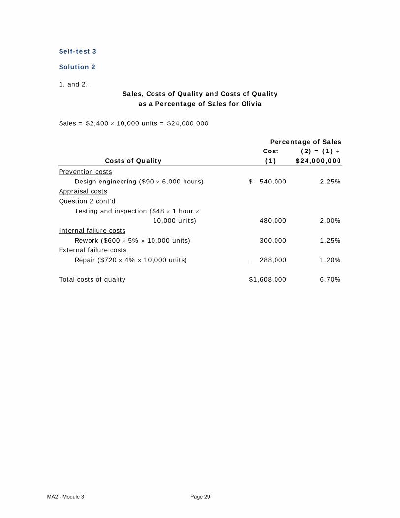
Solution 1

1. The ratio of each COQ category to revenues for each period is as follows:

Semi-annual Costs of Quality Report Bergen, Inc. (in thousands)

6/30/2007 12/31/2007 6/30/2008 12/31/2008 % of Rev. % of Rev. % of Rev. % of Rev. (2) = (4) = (6) = (8) = (1) (1)÷4,944 (3) (3)÷5,448 (5) (5)÷5,580 (7) (7)÷5,412 Prevention costs Machine maintenance$ 258 $ 258 $ 228 $ 192 Training suppliers 6 54 24 18 Design reviews 24 122 120 114 288 5.8% 434 8.0% 372 6.7% 324 6.0% Appraisal costs Incoming inspection 54 64 43 26 Final testing 192 192 168 113 246 5.0% 256 4.7% 211 3.8% 139 2.6% Internal failure costs Rework 144 127 106 74 Scrap 82 77 50 48 226 4.6% 204 3.7% 156 2.8% 122 2.2% External failure costs Warranty repairs 83 37 30 28 Customer returns 314 301 139 96 397 8.0% 338 6.2% 169 3.0% 124 2.3% Total quality costs $1,157 23.4% $1,232 22.6% $ 908 16.3% $ 709 13.1% Total production and revenues $4,944 $5,448 $5,580 $5,412

From an analysis of the Cost of Quality Report, it would appear that Bergen Inc.’s program has been successful since • Total quality costs as a percentage of total revenues have declined from 23.4%

to 13.1%. • External failure costs, those costs signaling customer dissatisfaction have

declined from 8% of total revenues to 2.3%. These declines in warranty repairs and customer returns should translate into increased revenues in the future.

• Internal failure costs have been reduced from 4.6% to 2.2% of revenues. • Appraisal costs have decreased from 5.0% to 2.6%. Preventing defects from

occurring in the first place is reducing the demand for final testing. • Quality costs have shifted to the area of prevention where problems are solved

before production starts. Maintenance, training, and design reviews have increased from 5.8% of total revenues to 6% and from 24.9% of total quality costs ($288 ÷ $1,157) to 45.7% ($324 ÷ $709). The $36,000 increase in these costs is more than offset by decreases in other quality costs.


Because of improved designs, quality training, and additional pre-production inspections, scrap and rework costs have declined. Production does not have to spend an inordinate amount of time with customer service since they are now making the product right the first time and warranty repairs and customer returns have decreased.

2. To measure the opportunity cost of not implementing the quality program, Bergen

Inc. could assume that

• Sales and market share would continue to decline if the quality program had not been implemented and then calculate the loss in revenue and contribution margin.

• The company would have to compete on price rather than quality and calculate the impact of having to lower product prices.

Opportunity costs are not recorded in accounting systems because they represent the results of what might have happened if Bergen had not improved quality. Nevertheless, opportunity costs of poor quality can be significant. It is important for Bergen to take these costs into account when making decisions about quality.


Self-test 3

Solution 2

1. and 2. Sales, Costs of Quality and Costs of Quality

as a Percentage of Sales for Olivia Sales = $2,400 × 10,000 units = $24,000,000 Percentage of Sales Cost (2) = (1) ÷ Costs of Quality (1) $24,000,000

Prevention costs Design engineering ($90 × 6,000 hours) $ 540,000 2.25% Appraisal costs Question 2 cont’d Testing and inspection ($48 × 1 hour × 10,000 units) 480,000 2.00% Internal failure costs Rework ($600 × 5% × 10,000 units) 300,000 1.25% External failure costs Repair ($720 × 4% × 10,000 units) 288,000 1.20% Total costs of quality $1,608,000 6.70%


Sales, Costs of Quality and Costs of Quality as a Percentage of Sales for Solta

Sales: $1,800 × 5,000 units = $9,000,000 Percentage of Sales Cost (2) = (1) ÷ Costs of Quality (1) $9,000,000

Prevention costs Design engineering ($90 × 1,000 hours) $ 90,000 1.00% Appraisal costs Testing and inspection ($48 × 0.5 × 5,000 units) 120,000 1.33% Internal failure costs Rework ($480 × 10% × 5,000 units) 240,000 2.67% External failure costs Repair ($540 × 8% × 5,000 units) 216,000 2.40% Estimated forgone contribution margin on lost sales [($1,800 – $960) × 300] 252,000 2.80% Total external failure costs 468,000 5.20% Total costs of quality $918,000 10.20% Costs of quality as a percentage of sales are significantly different for Solta (10.20%) as compared with Olivia (6.70%). Ontario spends very little on prevention and appraisal activities for Solta, and incurs high costs of internal and external failures. Ontario follows a different strategy with respect to Olivia, spending a greater percentage of sales on prevention and appraisal activities. The result: fewer internal and external failure costs and lower overall costs of quality as a percentage of sales than with Solta. 3. Examples of nonfinancial quality measures that Ontario Industries could monitor

as part of a total-quality-control effort are (a) Outgoing quality yield for each product. (b) Returned refrigerator percentage for each product. (c) On-time delivery. (d) Employee turnover.


Self-test 3

Solution 3

1. If the branch expects to receive 60 customers each day and it takes 4.5 minutes

to serve a customer, the average time that a customer will wait in line before being served is:

( )( )

( )( )

260 4.5 60 20.25 60 20.25 1, 215 20.25 minutes2 300 270 2 30 602 300 60 4.5

⎡ ⎤× × ×⎣ ⎦= = = = =× − ×× − ×⎡ ⎤⎣ ⎦

2. Suppose the bank counter is kept open for X minutes. Then we want

( )( )

260 4.5 5 minutes2 X 60 4.5

⎡ ⎤×⎣ ⎦= =× − ×⎡ ⎤⎣ ⎦

that is, 60 × 20.25 = 10(X – 270) X – 270 = (60 × 20.25) ÷ 10 = 121.5 X = 391.5 minutes

The counter must be kept open for 391.5 minutes to reduce average waiting time to 5 minutes.1

3. Incremental operating income from providing new services $36 Incremental teller cost (2 additional hours × $12 per hour)2 24 Net increase in operating income from providing new services $12

Yes, the bank should offer the new services since the relevant benefits exceed the relevant costs.3

1) The assumption here is that the customer rate (# of customers per hour) is constant. 2) 91.5 minutes or a little over 1.5 hours of teller time have to be added. Since tellers are paid in increments of an hour, this means 2 additional hours of incremental teller cost. 3) The assumption here is that only variable labour costs matter. However, if variable

and/or fixed overhead costs changed upwards as a result of the extra 1.5 hours of operating time, gross margin analysis would be required.


Self-test 3

Solution 4

1. Finishing is a bottleneck operation. Hence, producing 1,000 more units will

generate additional throughput contribution and operating income.

Increase in throughput contribution ($86.40 – $38.40) × 1,000 $48,000 Incremental costs of the jigs and tools 36,000 Net benefit of investing in jigs and tools $12,000

Mayfield should invest in the modern jigs and tools because the benefit of higher throughput contribution of $48,000 exceeds the cost of $36,000.

2. The Machining Department has excess capacity and is not a bottleneck operation.

Increasing its capacity further will not increase throughput contribution. There is therefore no benefit from spending $6,000 to increase the Machining Department’s capacity by 10,000 units. Mayfield should not implement the change to do setups faster.


Self-test 3

Solution 5

1. SRG expects to use 4,800 (96 hours per order × 50 orders) hours of total capacity

of 6,000 hours equal to 4,800 80%.6,000

=

2. Average manufacturing lead time for Z39

Average waiting time = (average number of orders of Z39 x (manufacturing time for Z39)2) ÷ 2 x [annual machine capacity – (average number of orders of Z39 x manufacturing time for Z39)]

= ( )

( )( ) ( )

250 96 50 9, 216 460,800 192 hours2 6,000 4,800 2 1,2002 6,000 50 96

⎡ ⎤× ×⎣ ⎦ = = =× − ×× − ×⎡ ⎤⎣ ⎦


time for Z39lead time for Z39 time for Z39

192 hours + 96 hours = 288 hours (12 days)

= +

=

3. Average waiting time for Z39 and Y28

= {[(average number of orders of Z39) x (manufacturing time for Z39)2] + [(average number of orders of Y28) x (manufacturing time for Y29)2]} ÷{2 x [annual machine capacity – [(average number of orders of Z39) x (manufacturing time for Z39)] –[(average number of orders of Y28) x (manufacturing time for Y28)]}

( ) ( )( ) ( )

( ) ( )[ ]

( )2 250 96 25 24 50 9, 216 25 576 460,800 14, 400

2 6,000 4,800 600 2 6002 6,000 50 96 25 24

475, 200 396 hours1, 200

⎡ ⎤ ⎡ ⎤× + × × + ×⎡ ⎤ +⎣ ⎦ ⎣ ⎦ ⎣ ⎦= = =× − − ×× − × − ×⎡ ⎤⎣ ⎦

= =


timelead time for Z39 time for Z39


= +

=



timelead time for Y28 time for Y28


= +

=

4. Average waiting time 396 94%

Average throughput time for Y28 420= =

Part Y28 spends 94% of the time in the plant, on average, just waiting to be processed!

5. Delays occur in the processing of Z39 and Y28 because (1) uncertainty about how

many orders SRG will actually receive (SRG expects to receive 50 orders of Z39 and 25 orders of Y28) and (2) uncertainty about the actual dates when SRG will receive the orders. The uncertainty (randomness) about the quantity and timing of customer orders means that SRG may receive customer orders while another order is still being processed. Orders received while the machine is actually processing another order must wait in queue for the machine to be free. As average capacity utilization of the machine increases, there is less slack and a greater chance that a machine will be busy when another order arrives.


Self-test 3

Solution 6

1. The direct approach is to look at incremental revenues and incremental costs. Average selling price per order for Y28, which has average operating throughput time of 420 hours $ 9,600 Variable costs per order 6,000 Additional contribution per order from Y28 3,600 Multiply by expected number of orders × 25 Increase in expected contribution from Y28 $90,000

Expected loss in revenues and increase in costs from introducing Y28

Product

(1)

Expected Loss in Revenues from

Increasing Average Manufacturing Lead

Times for All Products

(2)

Expected Increase in Carrying Costs from Increasing

Average Manufacturing

Lead Times for All Products

(3)

Expected Loss in Revenues Plus

Expected Increases in

Costs of Introducing

Y28 (4) = (2) + (3)

Z39 Y28 Total

$30,000a — .

$30,000

$ 7,650b 2,625c $10,275

$37,650 2,625 $40,275

a50 orders × ($32,400 – $31,800) b(492 hours – 288 hours) × $0.75 × 50 orders c(420 hours – 0) × $0.25 × 25

Increase in expected contribution from Y28 of $90,000 is greater than increase in expected costs of $40,275 by $49,725. Therefore, SRG should introduce Y28.


Alternative calculations of incremental revenues and incremental costs of introducing Y28.

Alternative 1: Introduce Y28

(1)

Alternative 2: Do Not

Introduce Y28 (2)

Relevant Revenues and Relevant Costs (3) = (1) – (2)

Expected revenues Expected variable costs Expected carrying costs Expected total variable and

carrying costs Expected revenues minus

expected costs

$1,830,000a 1,050,000c

21,075e

1,071,075

$ 758,925

$1,620,000b 900,000d

10,800f

910,800

$ 709,200

$210,000 150,000

10,275

160,275

$ 49,725

a(50 × $31,800) + (25 × $9,600) b50 × $32,400 c(50 × $18,000) + (25 × $6,000) d50 × $18,000 e(50 × $0.75 × 492) + (25 × $0.25 × 420) f50 × $0.75 × 288

2. Introducing Y28 results in an incremental cost of $40,275. To break even, you

need to earn a total contribution of $40,275 over the 25 orders, or a contribution per order of $40,275 ÷ 25 = $1,611.

Variable costs per order of Y28 $6,000 Required contribution to break even 1,611 Selling price per dollar of Y28 to break even $7,611

If Y28 sells above $7,611 per order, SRG should manufacture and sell Y28. If Y28 sells below $7,611 per order, SRG should not manufacture and sell Y28.


Date post:	24-Jun-2018
Category:	Documents
Upload:	truongtu
View:	213 times
Download:	0 times

Module 3: Quality and timecga-education.org/2009-10/ma2/module03.pdf · 2009-02-23 · You learn...

Documents