160
Molecular dynamics simulation of graphene formation on 6H–SiC substrate via simulated annealing Yoon Tiem Leong @ Min Tjun Kit School of Physics Universiti Sains Malaysia 1 Aug 2012
| Date post: | 07-Feb-2018 |
| Category: |
Documents |
| Upload: | nguyendiep |
| View: | 234 times |
| Download: | 4 times |
Molecular dynamics
simulation of graphene
formation on 6H–SiC
substrate via simulated
annealing Yoon Tiem Leong @ Min Tjun Kit
School of Physics
Universiti Sains Malaysia
1 Aug 2012
Single layer graphene formation
How we construct the unit cell and
supercell for 6H-SiC substrate
We refer to
http://cst-
www.nrl.navy.mil/lattice/struk/6h.html to
construct our 6H-SiC substrate.

Figure 1: Snapshot from http://cst-www.nrl.navy.mil/lattice/struk/6h.html. The 6H-SiC
belongs to the hexagonal class. For crystal in such a class, the lattice parameters and the
angles between these lattice parameters are such that a = b c ; a = b = 90 degree, g =
120 degree.
The snapshots from the above
webpage

Figure 2: Snapshot from http://cst-
www.nrl.navy.mil/lattice/struk.xmol/
6h.pos

Structure of the unit cell Each unit cell of the 6H-SiC has a total of 12
basis atoms, 6 of them carbon, and 6 silicon.
Figure 2 display:
(1) The coordinates of these atoms (listed in the last 12 rows in Figure 2). We note that only the Cartesian coordinates are to be used when preparing the input data for LAMMPS.
(2) Primitive vectors a(1), a(2), a(3) in the {X, Y, Z} basis (i.e. Cartesian coordinate system).

Procedure to construct our
rhombus-shaped 6H-SiC
substrate First, we determine the lattice constants, a , b (= a),
c :
From Figure 2, the primitive vectors, a(1), a(2), a(3) are given respectively (in unit of nanometer) as
a(1) = (1.54035000, -2.66796446, 0 .00000000)
a(2) = (1.54035000, 2.66796446, 0.00000000)
a(3) = (.00000000, .00000000, 15.11740000).
Squaring a(1) and adding it to a(2) squared, we could easily obtain the value for the lattice parameter a, which is also equal to b by definition of the crystallographic group.
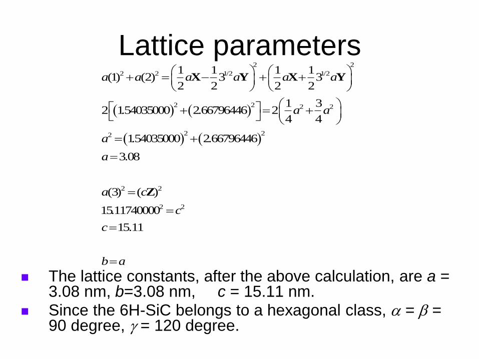
Lattice parameters
2 2
2 2 1/2 1/2
2 2 2 2
2 22
2 2
2 2
1 1 1 1(1) (2) 3 3
2 2 2 2
1 32 1.54035000 2.66796446 2
4 4
1.54035000 2.66796446
3.08
(3) ( )
15.11740000
15.11
a a a a a a
a a
a
a
a c
c
c
b a
X Y X Y
Z
The lattice constants, after the above calculation, are a = 3.08 nm, b=3.08 nm, c = 15.11 nm.
Since the 6H-SiC belongs to a hexagonal class, a = b = 90 degree, g = 120 degree.

Translation of lattice parameters
into LAMMPS-readable unit We refer to the instruction manual from
the LAMMPS website in order to feed
in the information of the lattice
parameters into LAMMPS:
http://lammps.sandia.gov/doc/Section_
howto.html#howto_12, section 6.12,
Triclinic (non-orthogonal) simulation
boxes
In LAMMPS, the units used are {lx, ly,
lz; xy, xz, yz}. We need to convert {a,
b, c; abg} into these units. This could
be done quite trivially, via the
conversion show in the right:

Raw unit cell of 6H-SiC
Based on the procedures described in
previous slides, we constructed a
LAMMPS data file for a raw 6H-SiC unit
cell.
It represents a unit cell of 6H-SiC
comprises of six hexagonal layers
repeating periodically in the z-direction.
The resultant data file, named
dataraw.xyz, is shown in Figure 4, to be
viewed using xcrysdens or VMD.
Raw unit cell of 6H-SiC
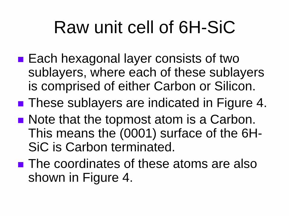
Each hexagonal layer consists of two sublayers, where each of these sublayers is comprised of either Carbon or Silicon.
These sublayers are indicated in Figure 4.
Note that the topmost atom is a Carbon. This means the (0001) surface of the 6H-SiC is Carbon terminated.
The coordinates of these atoms are also shown in Figure 4.
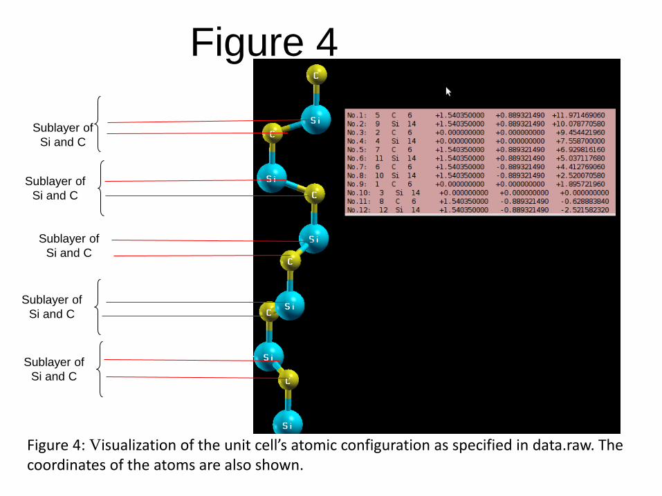
Figure 4: Visualization of the unit cell’s atomic configuration as specified in data.raw. The coordinates of the atoms are also shown.
Figure 4
Sublayer of
Si and C
Sublayer of
Si and C
Sublayer of
Si and C
Sublayer of
Si and C
Sublayer of
Si and C
Modification for carbon-rich
layer Next, we shall modify data.raw.xyz via the
following procedure:
The Si atom (No. 9) is removed. The atom
C (No. 5) is now translated along the z–
direction to take up the z-coordinate left
vacant by the removed Si atom (while the
x- and y-coordinate remains unchanged).
Content of data.singlelayer.xyz
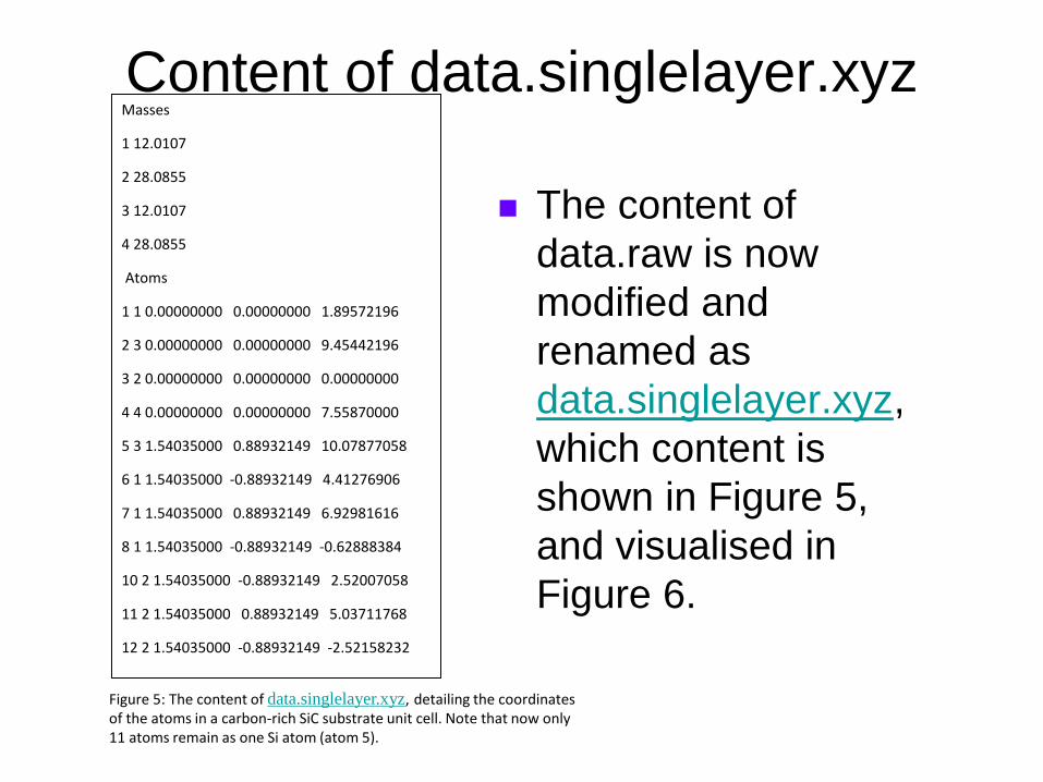
The content of
data.raw is now
modified and
renamed as
data.singlelayer.xyz,
which content is
shown in Figure 5,
and visualised in
Figure 6.
Masses
1 12.0107
2 28.0855
3 12.0107
4 28.0855
Atoms
1 1 0.00000000 0.00000000 1.89572196
2 3 0.00000000 0.00000000 9.45442196
3 2 0.00000000 0.00000000 0.00000000
4 4 0.00000000 0.00000000 7.55870000
5 3 1.54035000 0.88932149 10.07877058
6 1 1.54035000 -0.88932149 4.41276906
7 1 1.54035000 0.88932149 6.92981616
8 1 1.54035000 -0.88932149 -0.62888384
10 2 1.54035000 -0.88932149 2.52007058
11 2 1.54035000 0.88932149 5.03711768
12 2 1.54035000 -0.88932149 -2.52158232
Figure 5: The content of data.singlelayer.xyz, detailing the coordinates of the atoms in a carbon-rich SiC substrate unit cell. Note that now only 11 atoms remain as one Si atom (atom 5).

Figure 6. : Visualization of the unit cell’s atomic configuration as specified in data.singlelayer.xyz. This is the carbon-rich substrate to be used for single layer
graphene growth.
Figure 6: carbon-rich unit cell
of SiC
11 atoms per unit cell left
as one Si atom (No. 9) has
been removed.
Generating supercell
We then generated a supercell comprised
of 12 x 12 x 1 unit cells as specified in
data.singlelayer.xyz.
This is accomplished by using the
command
replicate 12 12 1
See the input script in.anneal (line 14 and
line 15).
Periodic BC
Periodic boundary condition is applied
along the x-, y- and z-directions via the
command ( in line 8, in.anneal):
boundary p p p
We created a vacuum of thickness 10 nm
(along the z-direction) above and below
the substrate.
The 12 x 12 x 1 supercell constructed
according to the above procedure is
visialised in Figure 7.
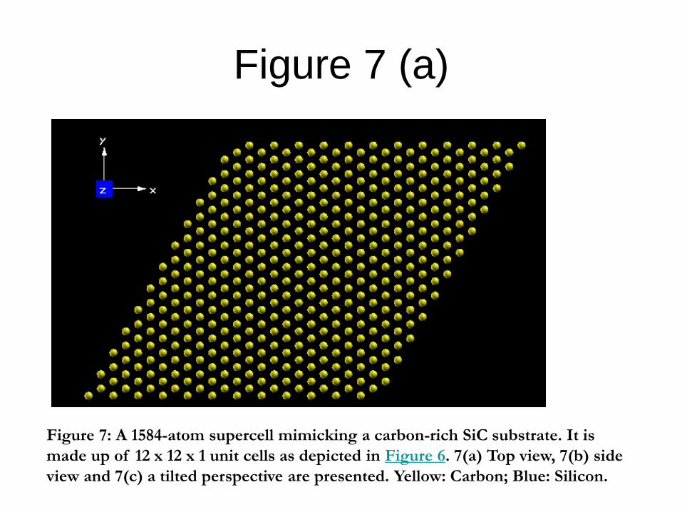
Figure 7 (a)
Figure 7: A 1584-atom supercell mimicking a carbon-rich SiC substrate. It is
made up of 12 x 12 x 1 unit cells as depicted in Figure 6. 7(a) Top view, 7(b) side
view and 7(c) a tilted perspective are presented. Yellow: Carbon; Blue: Silicon.

Figure 7 (b)

Figure 7 (c)
Visualisation of the 12 x 12 x 1
supercell There is a total of 1584 atoms in the simulation box.
Coordinates of all the atoms in the supercell can be obtained from LAMMPS‟s trajectory file during the annealing process.
These coordinates are simply the atomic coordinates of the first step output during the MD run.
View the structure file 10101.xyz using VMD.
Such a Carbon-rich substrate will be used as out input structure to LAMMPS to simulate epitaxial graphene growth.
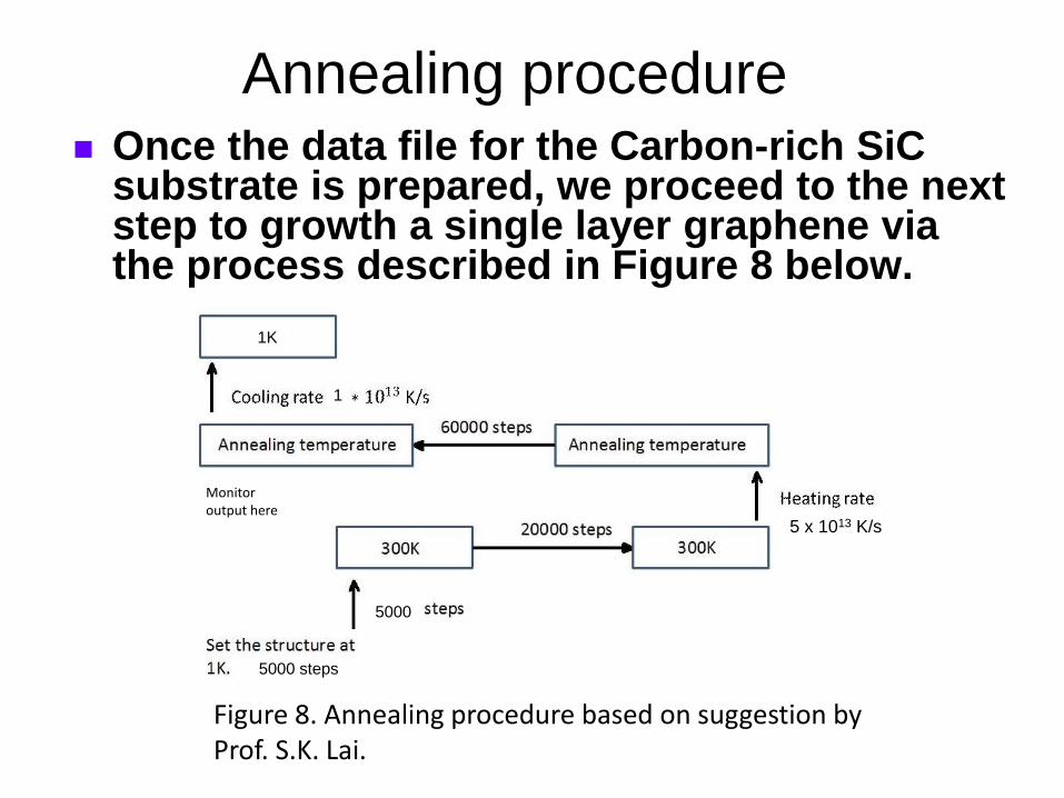
Annealing procedure
Figure 8. Annealing procedure based on suggestion by Prof. S.K. Lai.
Monitor output here
Once the data file for the Carbon-rich SiC substrate is prepared, we proceed to the next step to growth a single layer graphene via the process described in Figure 8 below.
5 x 10¹³ K/s
5000
1
1K
5000 steps

Implementation To implement the above procedure, a
fixed value of target annealing temperature was first chosen, e.g. Tanneal = 900 K.
For this fixed taret Tanneal, we ran the LAMMPS input script (in.anneal) to monitor the LAMMPS output while the system undergoes equilibration at the target annealing temperature (after the temperature has been ramped up gradually from 1 K).
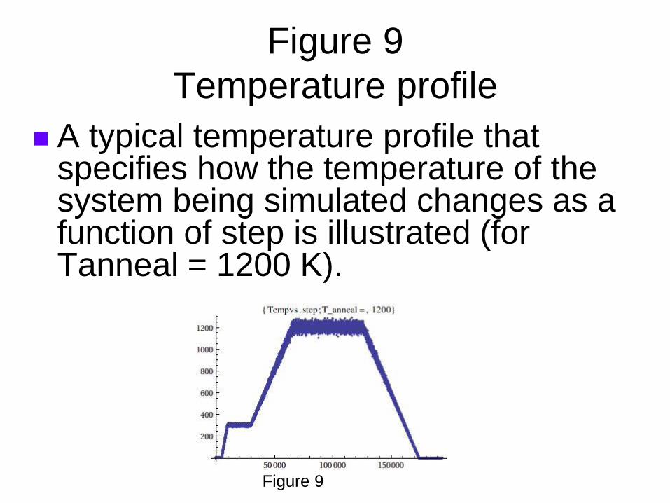
Figure 9
Temperature profile
A typical temperature profile that specifies how the temperature of the system being simulated changes as a function of step is illustrated (for Tanneal = 1200 K).
Figure 9
Implementation (cont.) Should graphene is formed at the target annealing
temperature, we shall observe the following phenomena during equilibrium (at that annealing temperature):
(i) An abrupt formation of hexagonal rings by the carbon rich layer (visualize the lammps trajectory file using VMD in video mode),
(ii) an abrupt drop of biding energy,
(iii) an abrupt change of pressure.
In actual running of the LAMMPS calculation, we repeat the above procedure for a set of selected target annealing temperature one-by-one, Tanneal = 400 K, 500K, 1100K, 1200 K …, 2000 K.
Numerical parameters The essential parameters used in annealing the substrate
for single layered graphene growth:
1. damping coefficient: 0.005
2. Timestep: 0.5 fs.
3. Heating rate from 300 K -> target temperatures, 5 x 10¹³ K/s.
4. Cooling rate: From target temperatures -> 1 K, 1 x 10¹³ K/s.
5. Target temperatures: 700 K, 800 K, …, 2000 K.
6. Steps for equilibration: (i) At 1K, 5000 steps. (ii) At 300 K, 20,000 steps, (iii) target annealing temp -> target annealing temp, 60,000 steps.
Essentially, all the parameters used are the same as that used by the NCU group.

Configuration of the carbon-rich substrate before and
after equilibration at T = 1.0 K for single-layered
graphene formation 0.624 Å
1.896 Å 0.2276 Å
1.9948 Å
Before
minimisation After
minimisation
0.63
Å 1.89
Å
0.22
Å
1.9
9Å
After minimization
but before
simulated annealing
As comparison, this figure shows the
geometry obtained by the NTCU group
before and after minimisation

Trajectory output • Trajectory output of the LAMMPS run with TEA
force filed for all Tanneal can be found in the directory /data/single/TEA.
• For example, dynamic formation of single-layered graphene on the SiC substrate for Tanneal = 1200 K can be viewed using VMD on the file 700_dynamicbonding_graphene.vmd (use the option File -> Load Visualizatioin State). This is a processed trajectory file in which dynamic bonding is enabled, and only the graphene layer is displayed (without substrate).
• The original LAMMPS trajectory file 1200.lammpstrj can be found in the same directory.
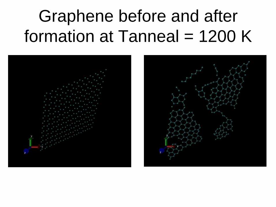
Graphene before and after
formation at Tanneal = 1200 K
Data and results for single layer
graphene formation The output for all Tannealing = {700K, 800K, …, 2000 K} are
displayed in Figures 10 for both TEA force fields.
In these graphs the following quantities are included:
(i) Temperature vs. step (tempvsstep.dat)
(ii) Binding energy versus step during equilibration at target annealing temperature (bindingenergyvsstep.dat).
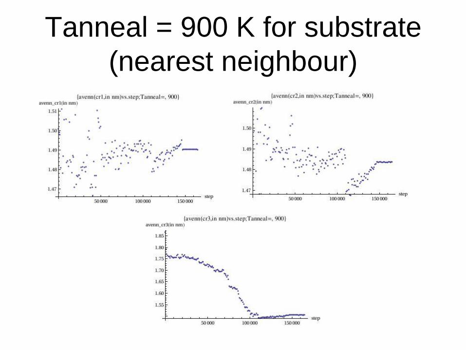
(iii) Average nearest neighbour of the topmost carbon atoms versus step during equilibration at target annealing temperature (avenn_vs_step.dat).
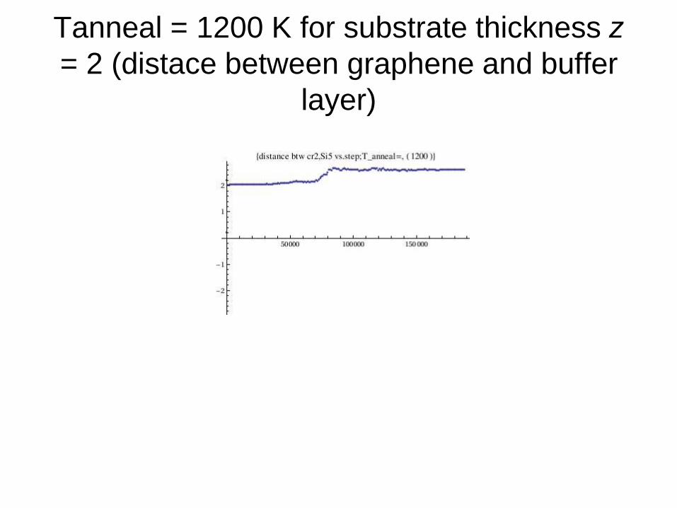
(iv) Average distance between the topmost carbon atoms and the Si atom lying just below these carbon atoms vs step (distance34vsstep.dat). This distance represents the “thickness” between the graphene and the substrate just below it (see next slide)
All these data are to be found in the directory /data/single.

Definition of d34 for single layer
graphene formation
Top carbon-rich layer
SiC substrate
d34 = average distance between the carbon-rich layer
and the substrate just below it
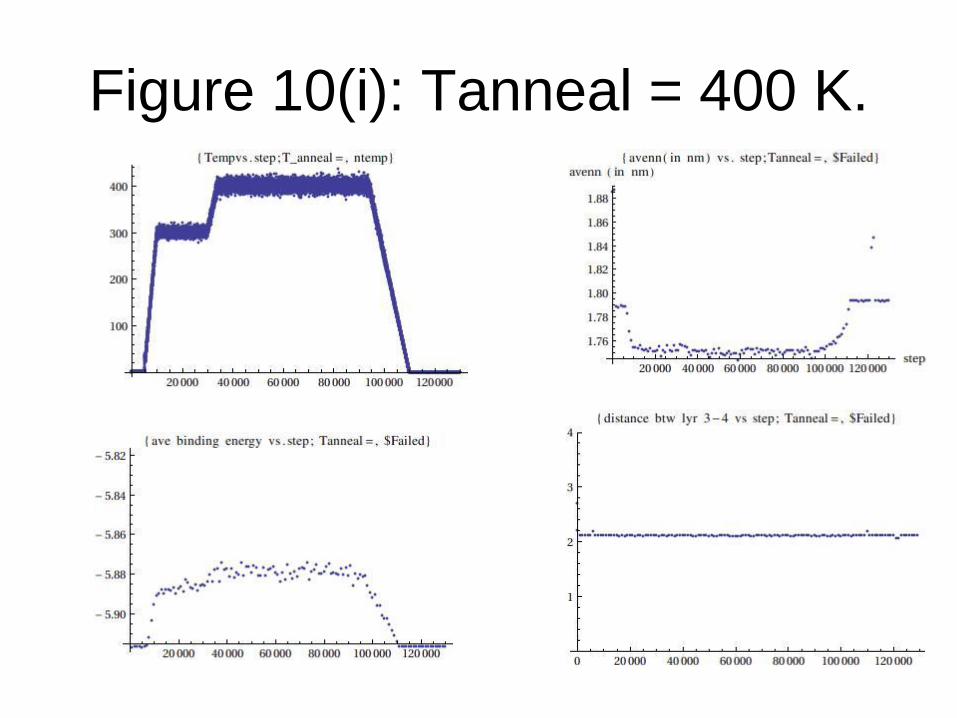
Figure 10(i): Tanneal = 400 K.
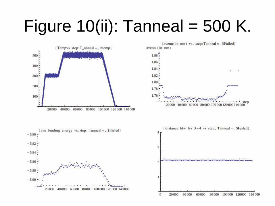
Figure 10(ii): Tanneal = 500 K.
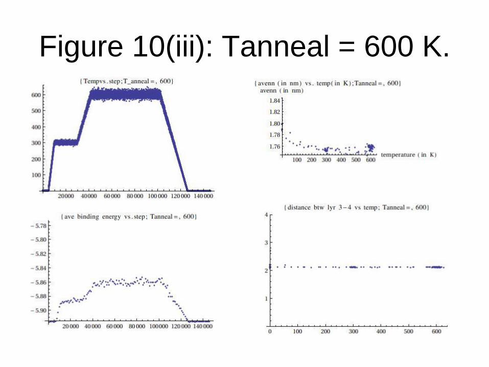
Figure 10(iii): Tanneal = 600 K.

Figure 10(iv): Tanneal = 700 K.
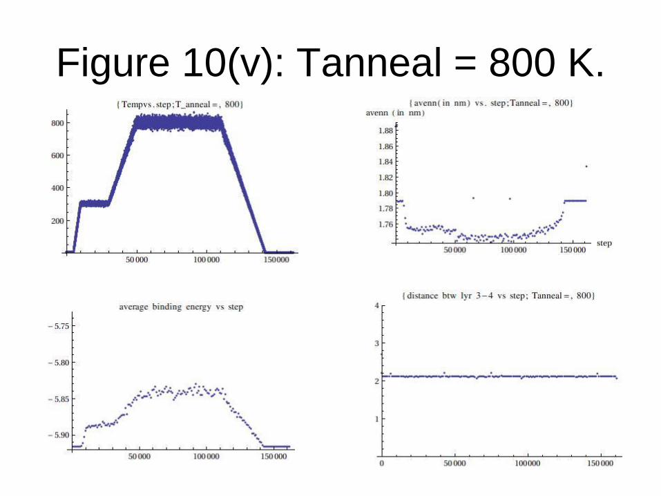
Figure 10(v): Tanneal = 800 K.

Figure 10(vi): Tanneal = 900 K.

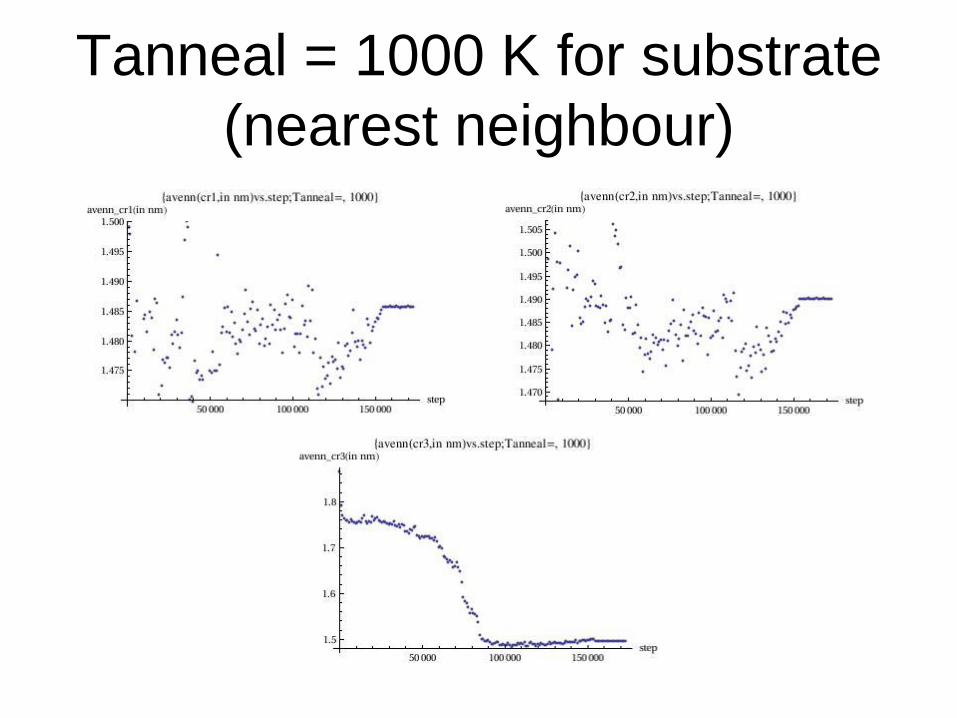
Figure 10(vii): Tanneal = 1000
K.
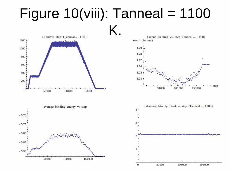
Figure 10(viii): Tanneal = 1100
K.

Figure 10(ix): Tanneal = 1200 K.
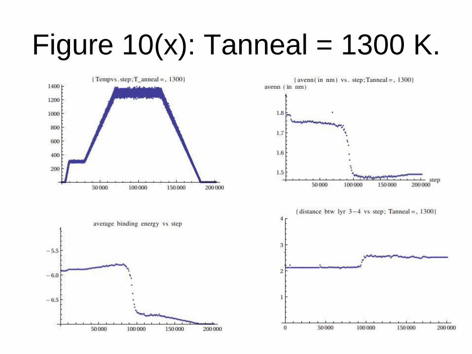
Figure 10(x): Tanneal = 1300 K.
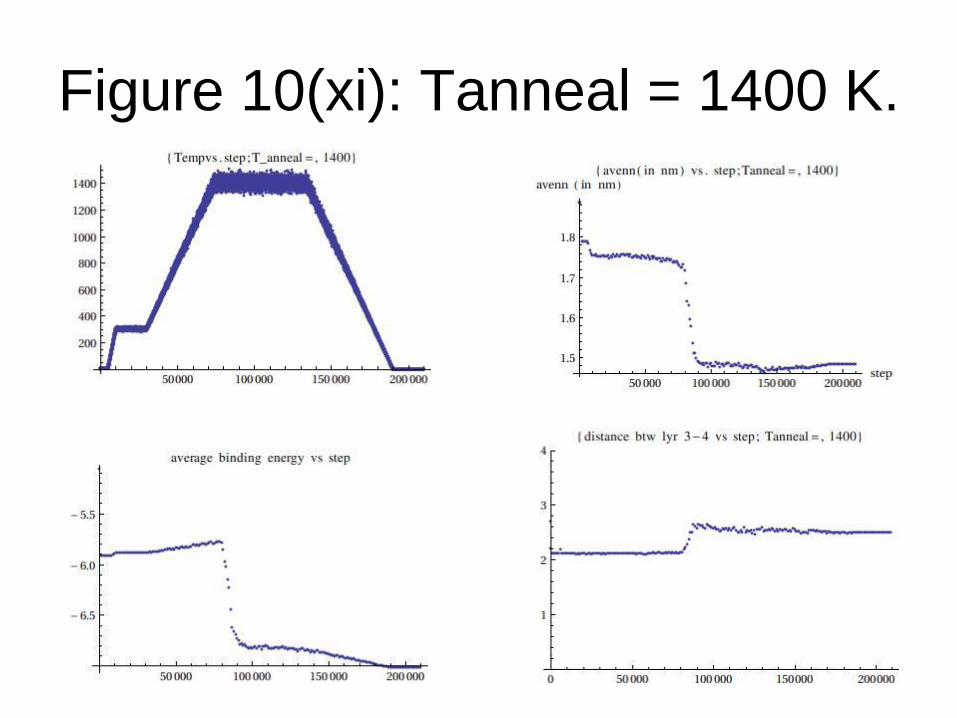
Figure 10(xi): Tanneal = 1400 K.
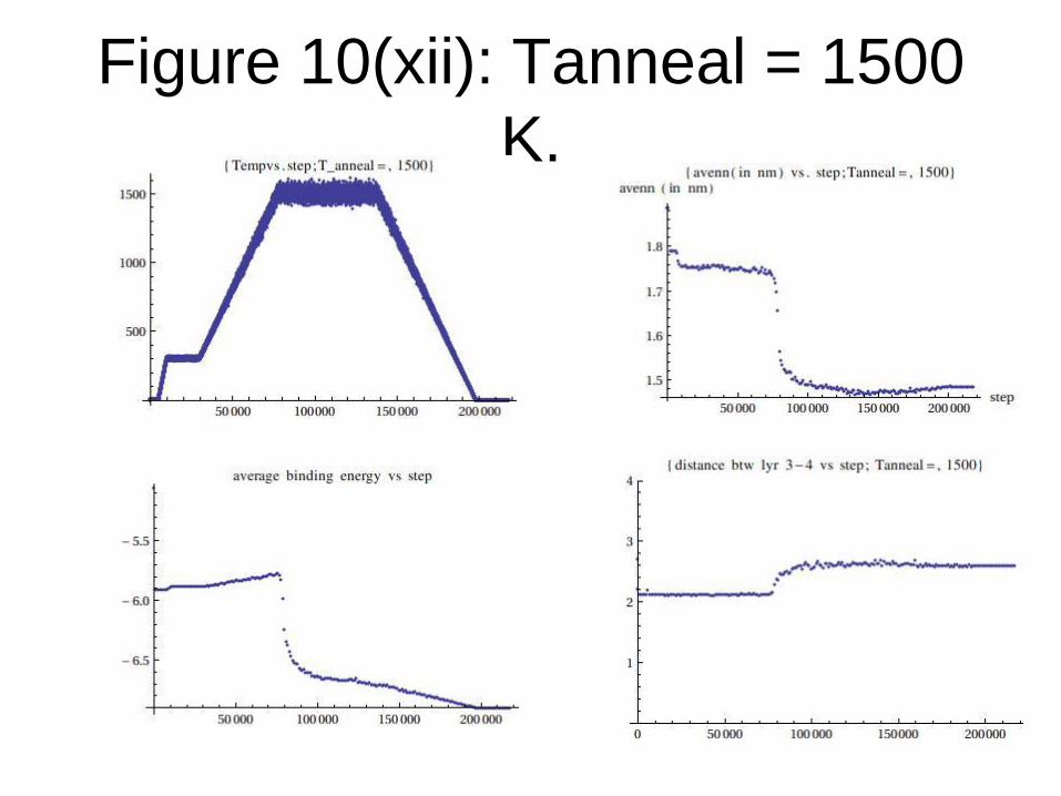
Figure 10(xii): Tanneal = 1500
K.

Figure 10(xiii): Tanneal = 1600
K.

Figure 10(xiv): Tanneal = 1700
K.
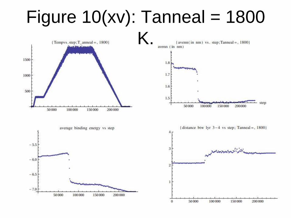
Figure 10(xv): Tanneal = 1800
K.
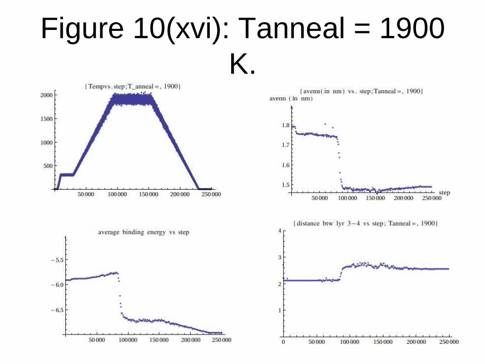
Figure 10(xvi): Tanneal = 1900
K.

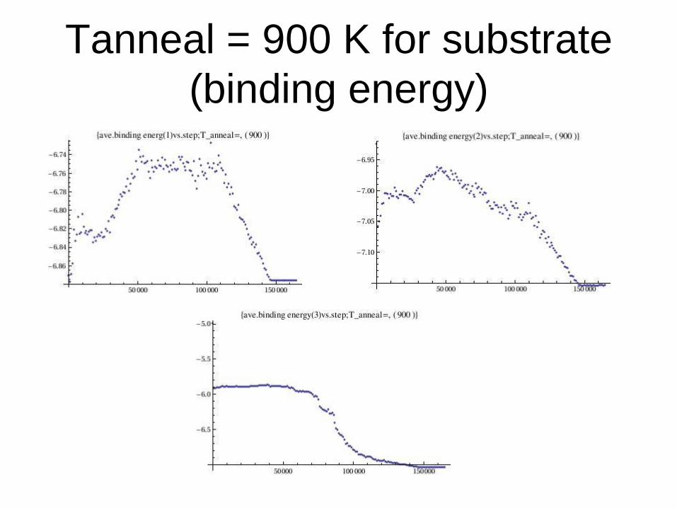
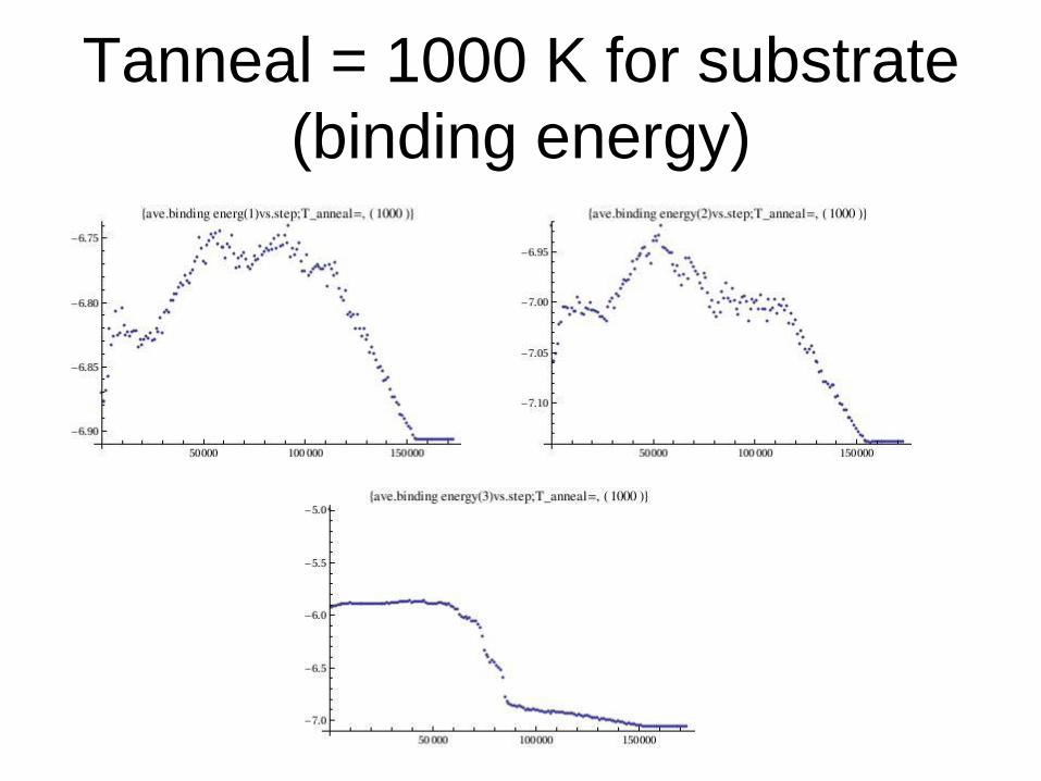
Determination of binding energy (BE)
Should an abrupt change in binding energy occurs at a given
Tanneal during equilibration, such as that illustrated below (for
Tanneal = 1200 K), how do we decide the value of the binding
energy (which is step-dependent) for this annealing
temperature?
Suggest to choose the value of the BE at the end of equilibration,
denoted as s. s is Tanneal-dependent:
s = 90000+(2/3)(Tanneal-300)
s s
BE vs. Tanneal
Based on the data shown in Figures 10, we
abstract the value of BE at step = s from
annealing temperature to plot the graph of
BE vs Tanneal.
The values of BE (at step s) vs Tanneal is
tabled in bdvstemp.dat.
The resultant curve is shown in Figure 11.

Anneal temp binding energy
400 -5.880829270833332
500 -5.868849618055552
600 -5.858356840277779
700 -5.853619340277778
800 -5.846055347222225
900 -5.831880138888886
1100 -5.817465729166667
1200 -5.808956701388889
1300 -5.99745027777778
1400 -6.751486666666667
1500 -6.5904123611111105
1600 -6.798648229166668
1700 -6.697513090277775
1800 -6.814728368055552
1900 -6.576965069444443
2000 -6.614329895833334
data\single\TEA\bdvstemp.dat
Binding energy vs anneal
temperature
Figure 11
Average nearest neighbour (nn) vs
anneal temperature
Based on the data shown in Figures 10, we
abstract the value of average nn at step = s
from each annealing temperature to plot the
graph of ave nn vs Tanneal.
The resultant curve is shown in Figure 12.

Anneal temp average nn
400 1.7506521837666498
500 1.7463308848628443
600 1.7535358998528505
700 1.7428323576363118
800 1.7434199844705522
900 1.755339645172511
1100 1.7324194569702076
1200 1.7287109331017865
1300 1.6587321720655723
1400 1.4872606748045474
1500 1.5048100430386822
1600 1.4789575688624732
1700 1.4770801292840978
1800 1.469249503109946
1900 1.4879246326794398
2000 1.4953312960924399
data\single\TEA\avennvstemp.dat
Average nearest neighbour (nn) vs
anneal temperature
Figure 12

Data and results for single layer
graphene formation
From the data generated, we conclude that:
Graphene formation is observed only when
Tanneal= Tf (transition temperature) = 1200
K or above for TEA potential.

Double-layered graphene
formation
55
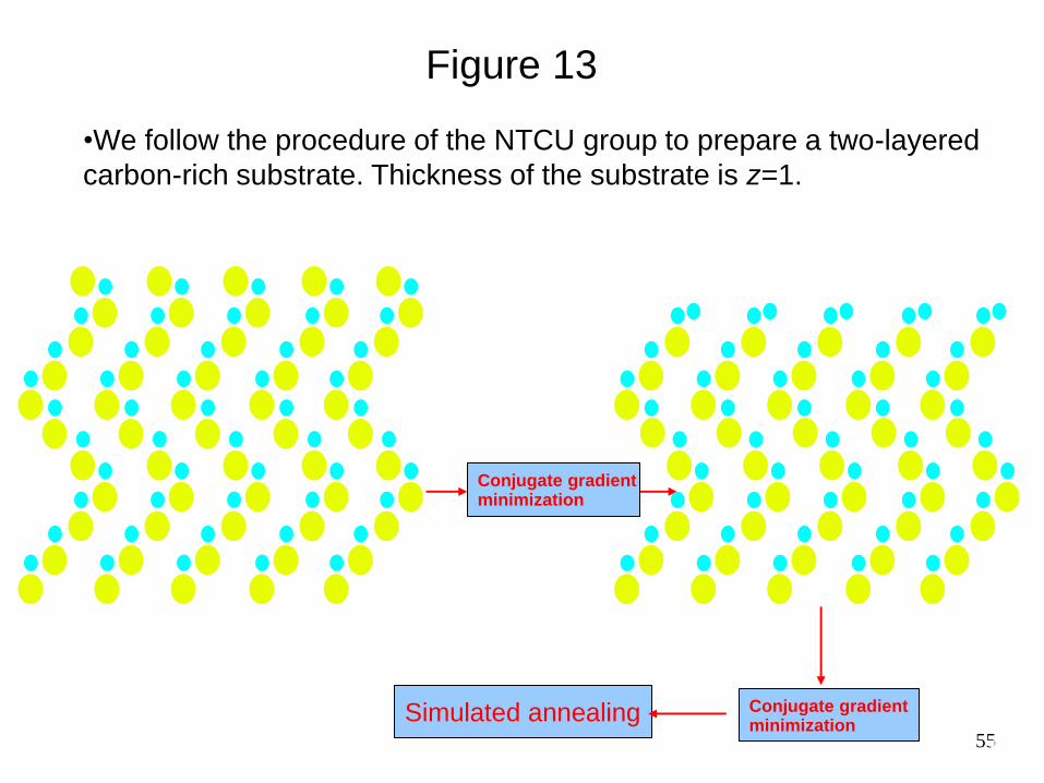
Figure 13
•We follow the procedure of the NTCU group to prepare a two-layered
carbon-rich substrate. Thickness of the substrate is z=1.
Conjugate gradient minimization
Simulated annealing Conjugate gradient minimization
14
Two-layered carbon-rich
substrate with
thickness z = 1
for double-layered graphene
formation
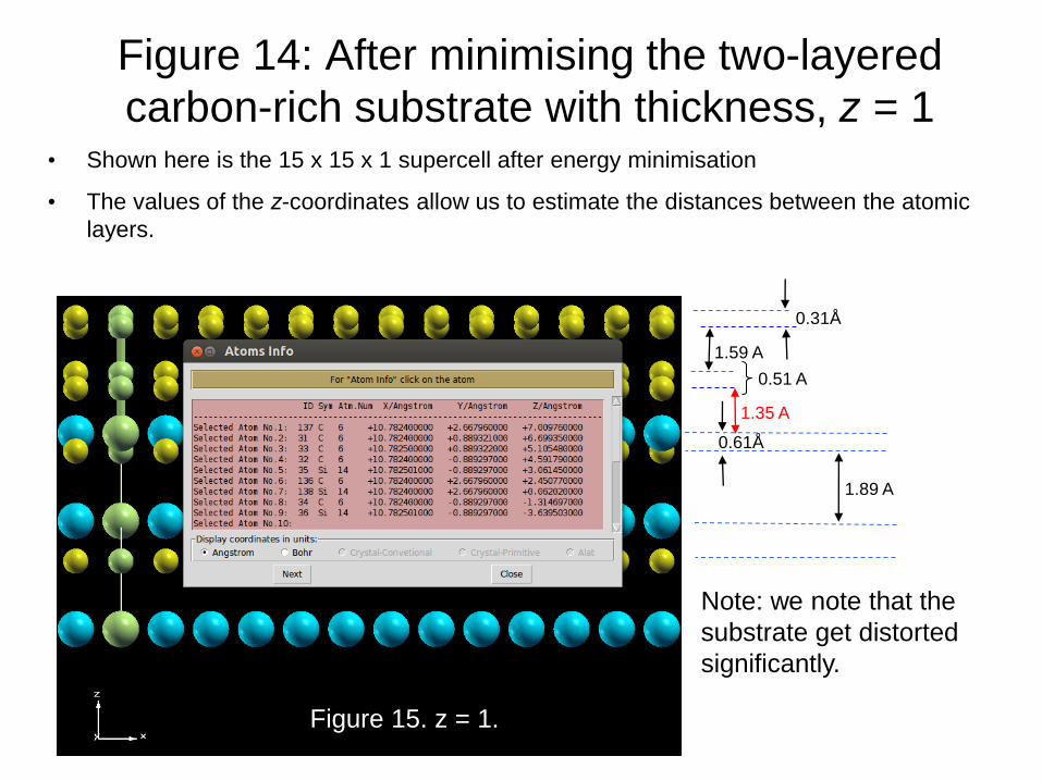
Figure 14: After minimising the two-layered
carbon-rich substrate with thickness, z = 1 • Shown here is the 15 x 15 x 1 supercell after energy minimisation
• The values of the z-coordinates allow us to estimate the distances between the atomic
layers.
0.31Å
0.61Å
1.89 A
1.59 A
0.51 A
1.35 A
Figure 15. z = 1.
Note: we note that the
substrate get distorted
significantly.

Visualising graphene formation for 15 x 15 x 1
supercell at Tanneal = 700 K, z = 1
We found that for substrate thickness z = 1, double-layered graphene is formed at as low as Tanneal = 600K.
The dynamical formation for Tanneal = 700 K can be visualised by viewing the following files with VMD, using option File -> „Load Visualization State‟. These are processed trajectory files where dynamic bonding option was enabled, with Distance Cutoff set to 1.7.
700_dynamicbonding_graphene.vmd
700_dynamicbonding_bulk.vmd
The original trajectory file 700.lammpstrj can be found in the same directory.
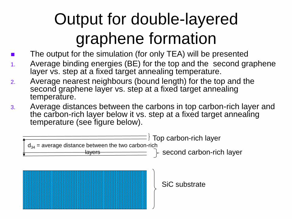
Output for double-layered
graphene formation The output for the simulation (for only TEA) will be presented
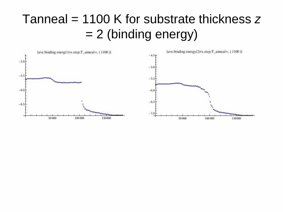
1. Average binding energies (BE) for the top and the second graphene layer vs. step at a fixed target annealing temperature.
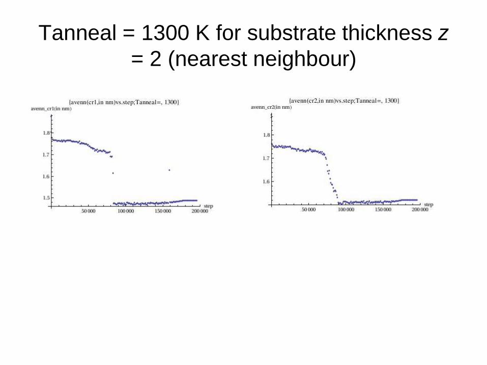
2. Average nearest neighbours (bound length) for the top and the second graphene layer vs. step at a fixed target annealing temperature.
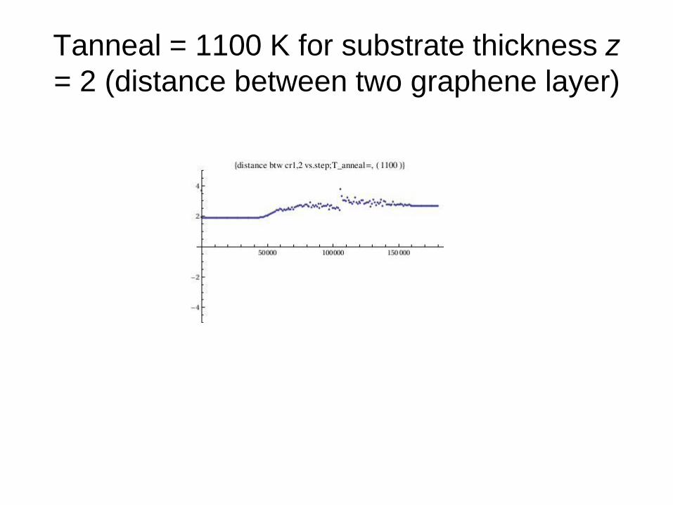
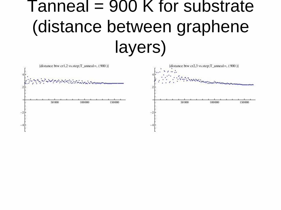
3. Average distances between the carbons in top carbon-rich layer and the carbon-rich layer below it vs. step at a fixed target annealing temperature (see figure below).
Top carbon-rich layer
second carbon-rich layer
SiC substrate
d34 = average distance between the two carbon-rich
layers
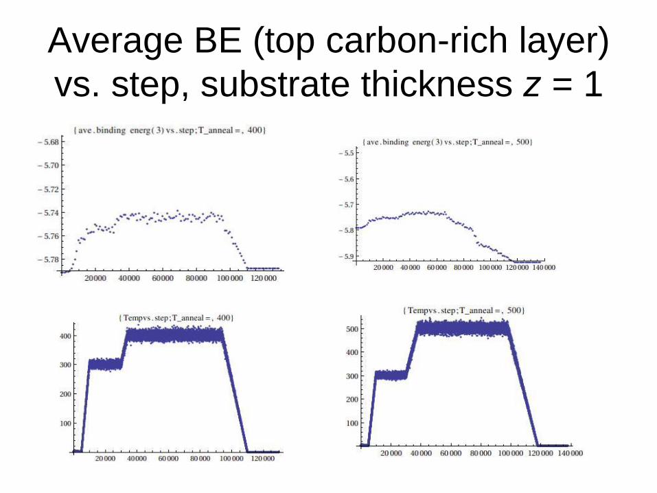
Average BE (top carbon-rich layer)
vs. step, substrate thickness z = 1
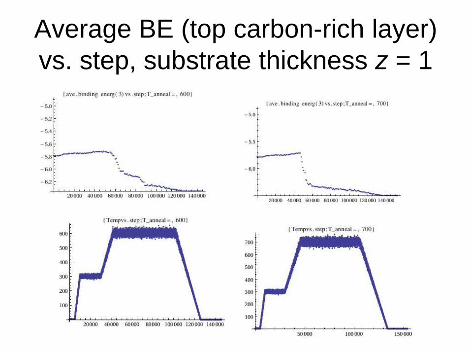
Average BE (top carbon-rich layer)
vs. step, substrate thickness z = 1
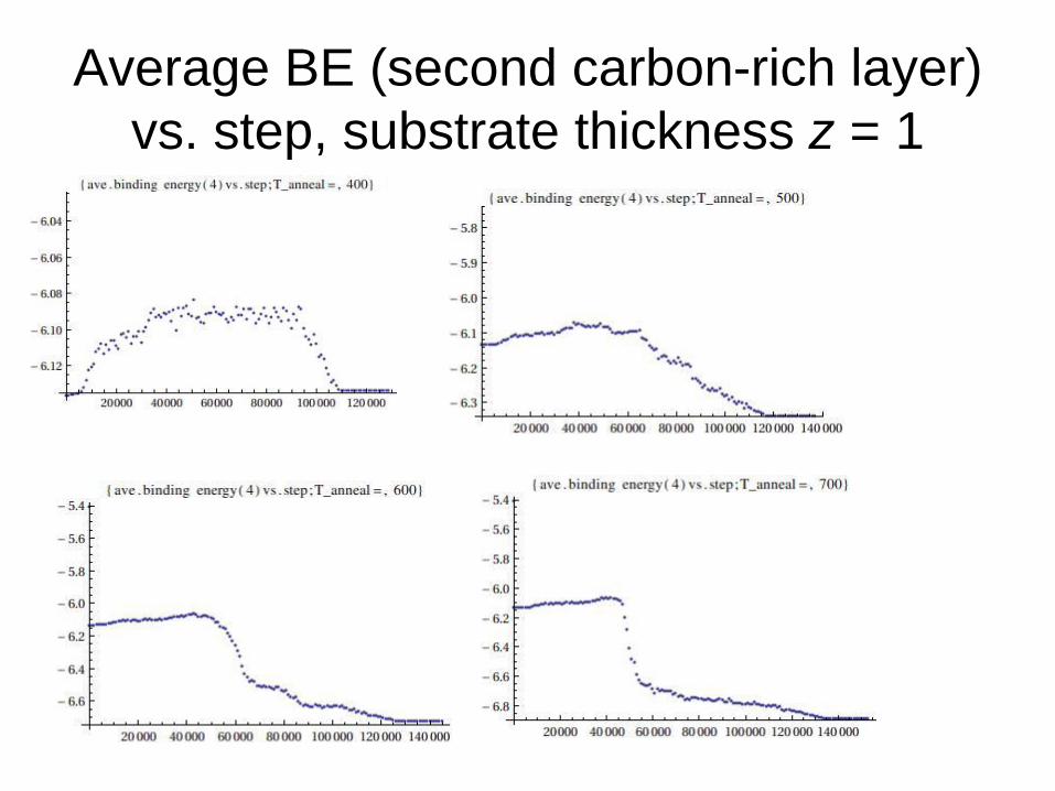
Average BE (second carbon-rich layer)
vs. step, substrate thickness z = 1
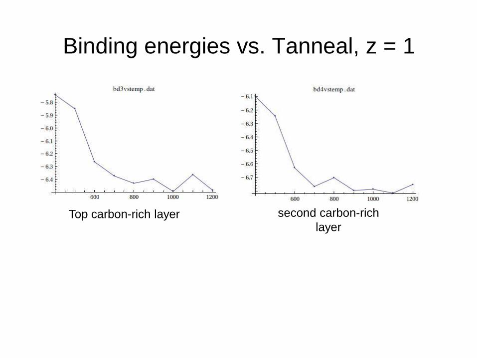
Binding energies vs. Tanneal, z = 1
Top carbon-rich layer second carbon-rich
layer
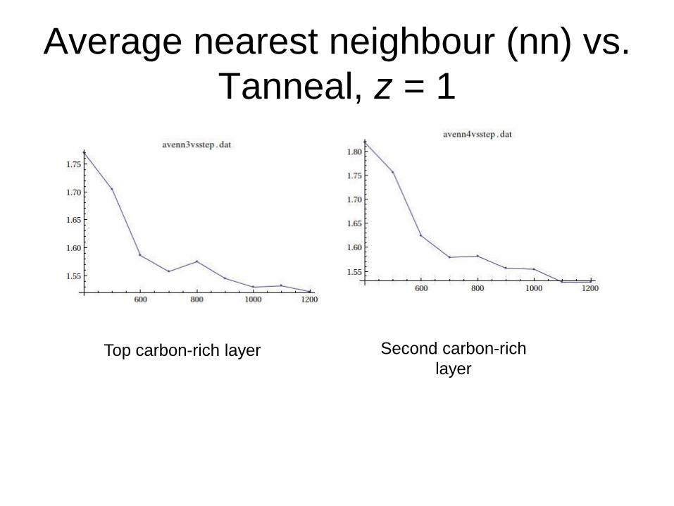
Average nearest neighbour (nn) vs.
Tanneal, z = 1
Top carbon-rich layer Second carbon-rich
layer

Average distance between the two
carbon-rich layers vs. Tanneal, z = 1
Location of data for z = 1
• The data for substrate thickness z = 1
double layered graphene formation can be
found in the folder \data\doublelayer\z1

Two-layered carbon-rich
substrate with
thickness z = 2
for double-layered graphene
formation
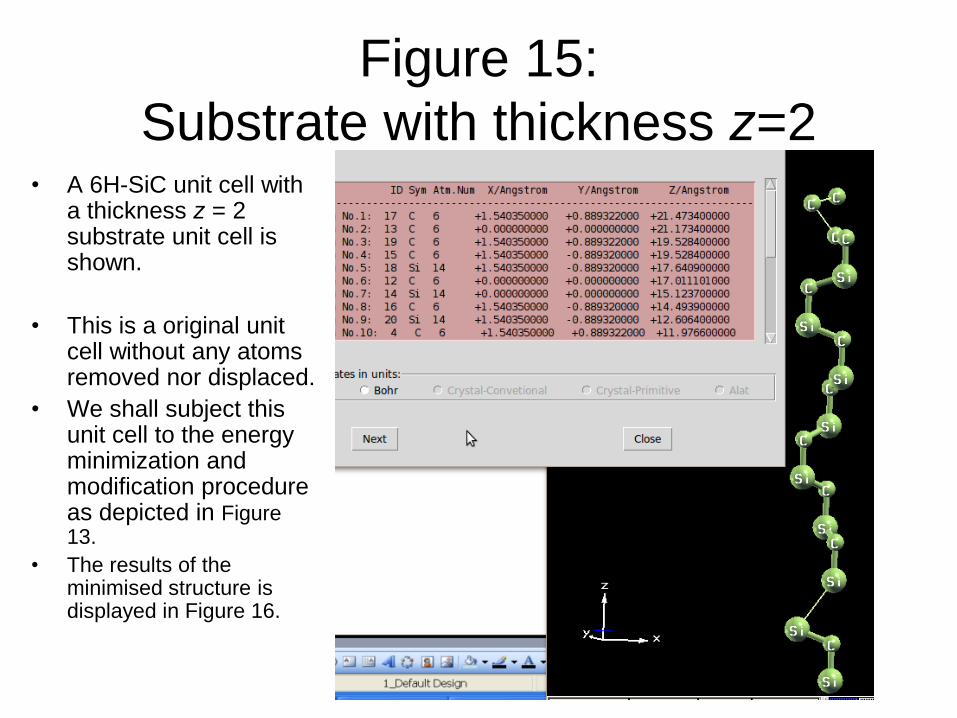
Figure 15:
Substrate with thickness z=2 • A 6H-SiC unit cell with
a thickness z = 2 substrate unit cell is shown.
• This is a original unit cell without any atoms removed nor displaced.
• We shall subject this unit cell to the energy minimization and modification procedure as depicted in Figure 13.
• The results of the minimised structure is displayed in Figure 16.
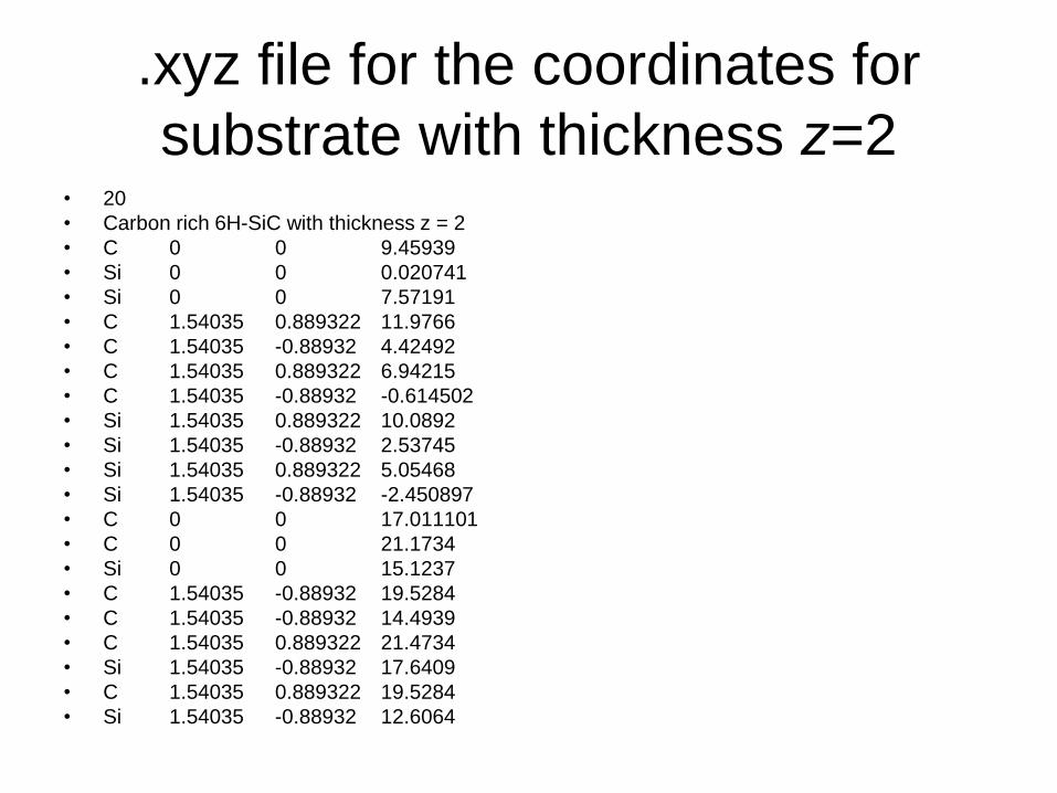
.xyz file for the coordinates for
substrate with thickness z=2 • 20
• Carbon rich 6H-SiC with thickness z = 2
• C 0 0 9.45939
• Si 0 0 0.020741
• Si 0 0 7.57191
• C 1.54035 0.889322 11.9766
• C 1.54035 -0.88932 4.42492
• C 1.54035 0.889322 6.94215
• C 1.54035 -0.88932 -0.614502
• Si 1.54035 0.889322 10.0892
• Si 1.54035 -0.88932 2.53745
• Si 1.54035 0.889322 5.05468
• Si 1.54035 -0.88932 -2.450897
• C 0 0 17.011101
• C 0 0 21.1734
• Si 0 0 15.1237
• C 1.54035 -0.88932 19.5284
• C 1.54035 -0.88932 14.4939
• C 1.54035 0.889322 21.4734
• Si 1.54035 -0.88932 17.6409
• C 1.54035 0.889322 19.5284
• Si 1.54035 -0.88932 12.6064
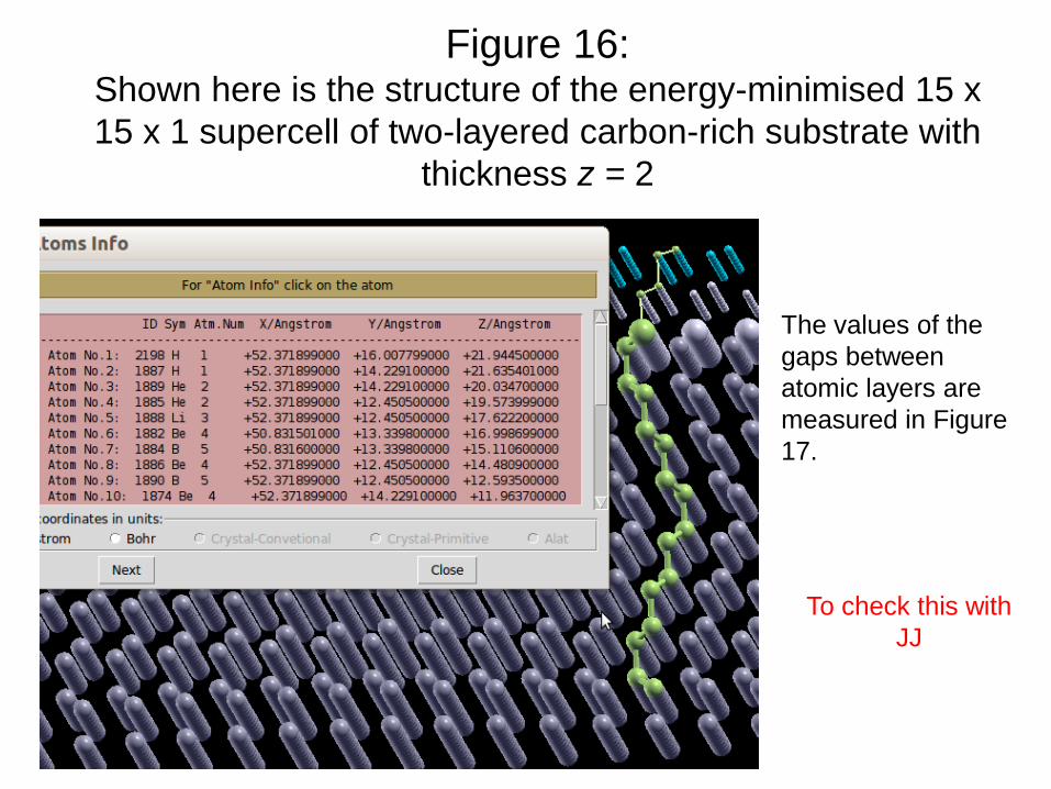
Figure 16: Shown here is the structure of the energy-minimised 15 x
15 x 1 supercell of two-layered carbon-rich substrate with
thickness z = 2
The values of the
gaps between
atomic layers are
measured in Figure
17.
To check this with
JJ
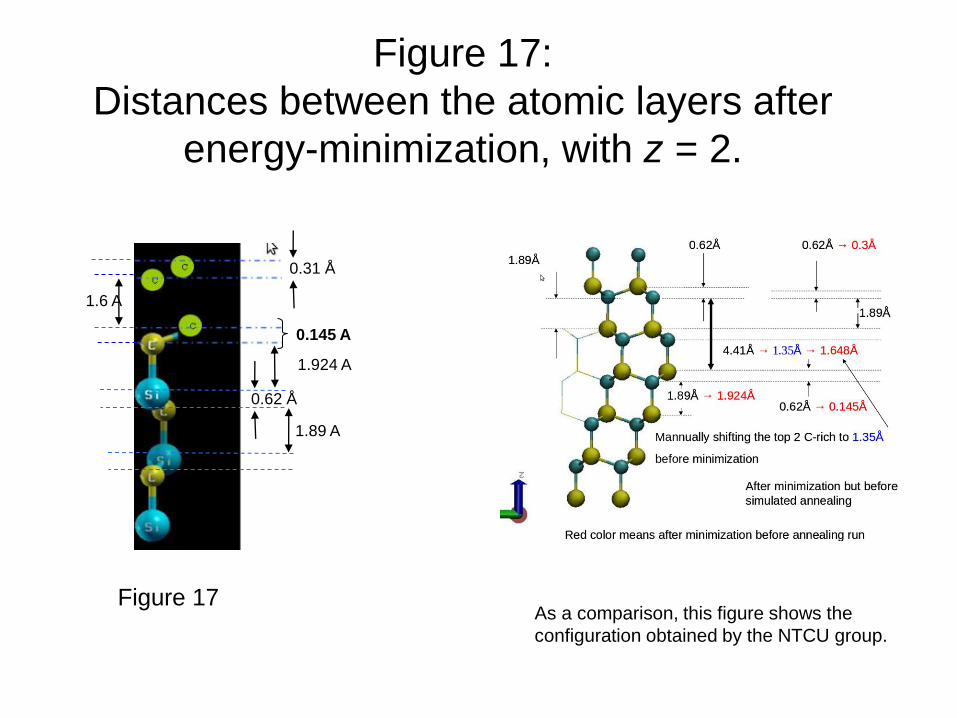
Figure 17:
Distances between the atomic layers after
energy-minimization, with z = 2.
0.31 Å
0.62 Å
1.89 A
1.6 A
As a comparison, this figure shows the
configuration obtained by the NTCU group.
0.145 A
1.924 A
Figure 17
Visualising graphene formation for 15 x 15 x 1
supercell at Tanneal = XXX K, z = 2
We found that for substrate thickness z = 2, double-layered graphene is formed at as low as Tanneal = xxx K.
The dynamical formation for Tanneal = xxx K can be visualised by viewing the following files with VMD, using option File -> „Load Visualization State‟. These are processed trajectory files where dynamic bonding option was enabled, with Distance Cutoff set to xx.
xxx_dynamicbonding_graphene.vmd
xxx_dynamicbonding_bulk.vmd
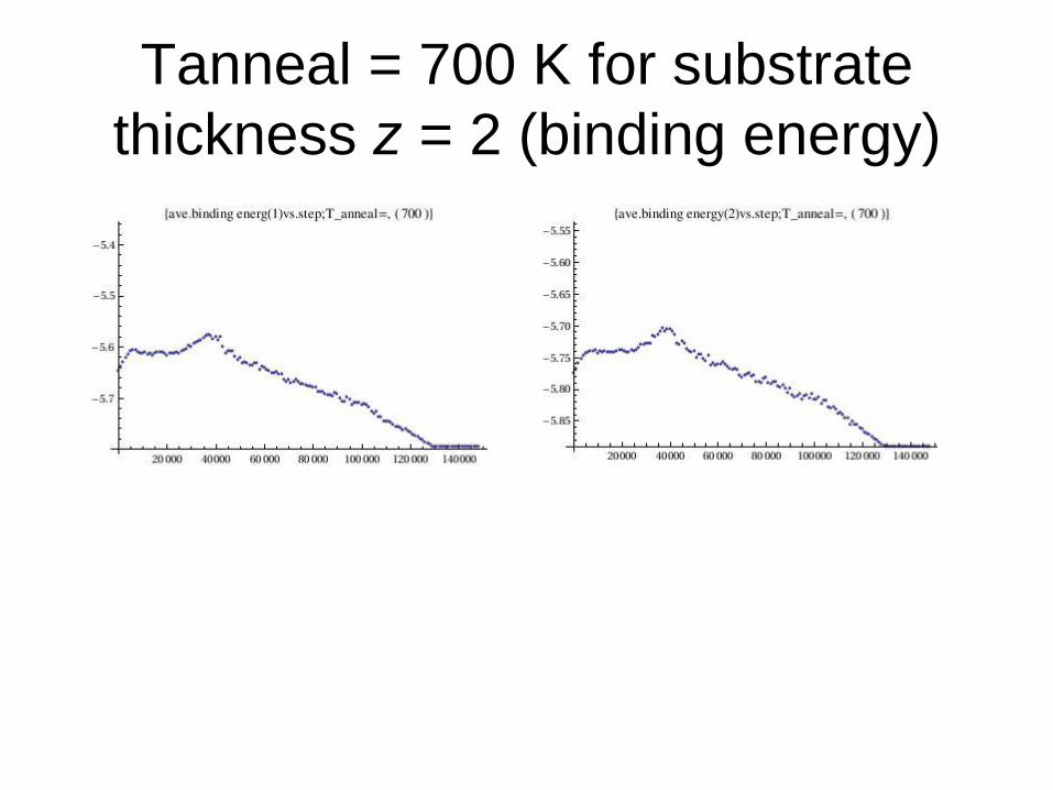
Tanneal = 700 K for substrate
thickness z = 2 (binding energy)
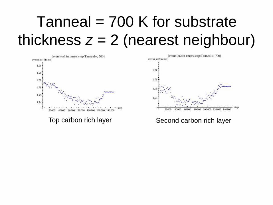
Tanneal = 700 K for substrate
thickness z = 2 (nearest neighbour)
Top carbon rich layer Second carbon rich layer
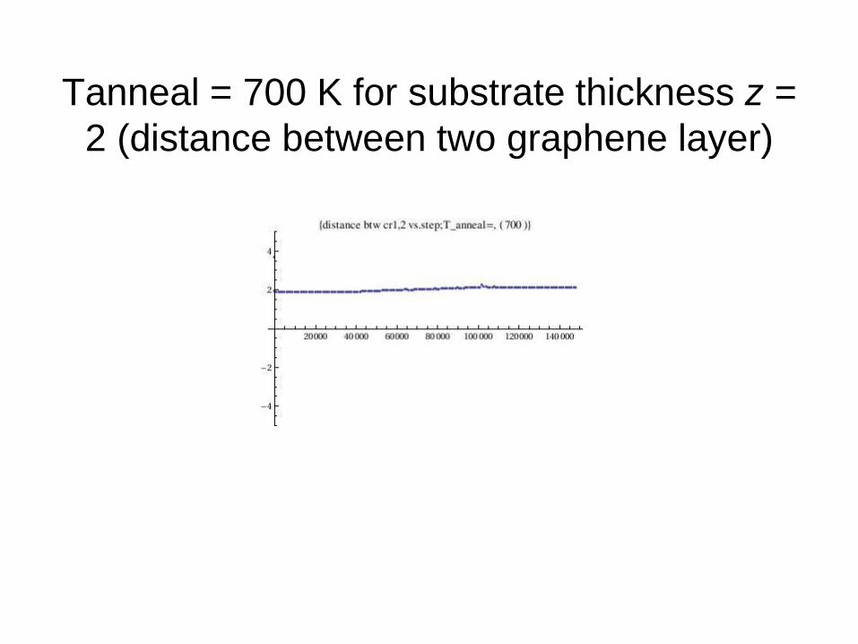
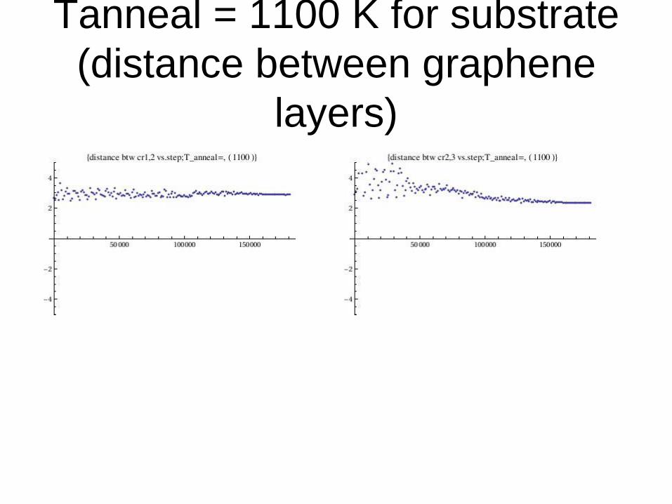
Tanneal = 700 K for substrate thickness z =
2 (distance between two graphene layer)
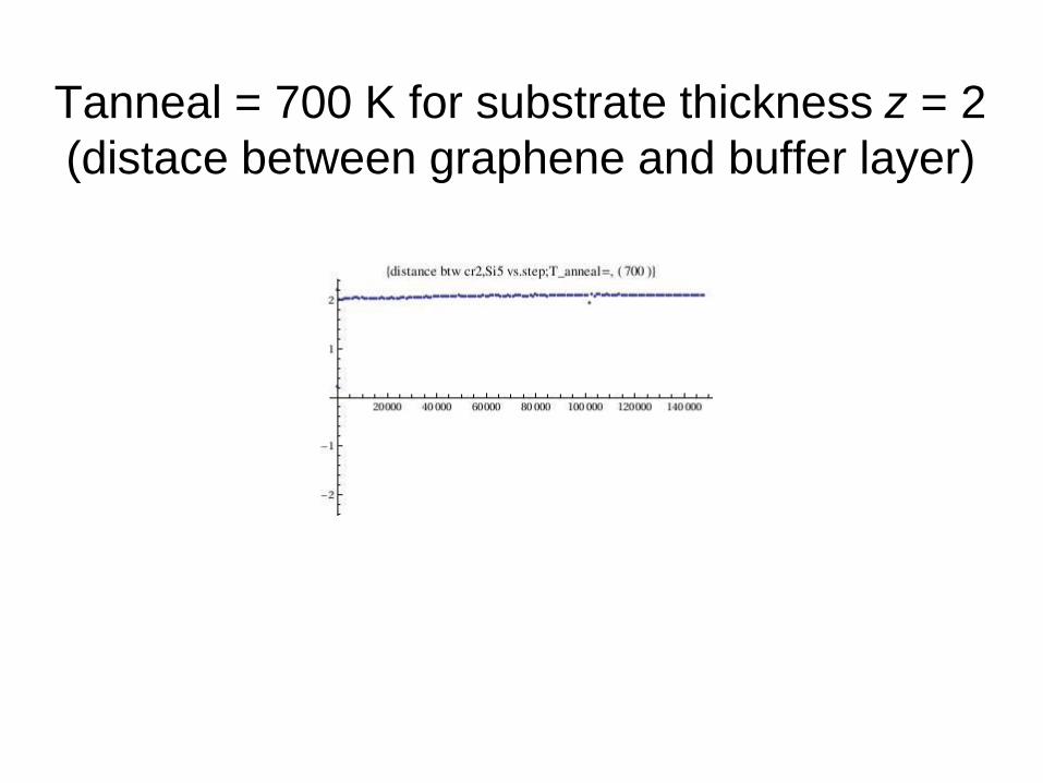
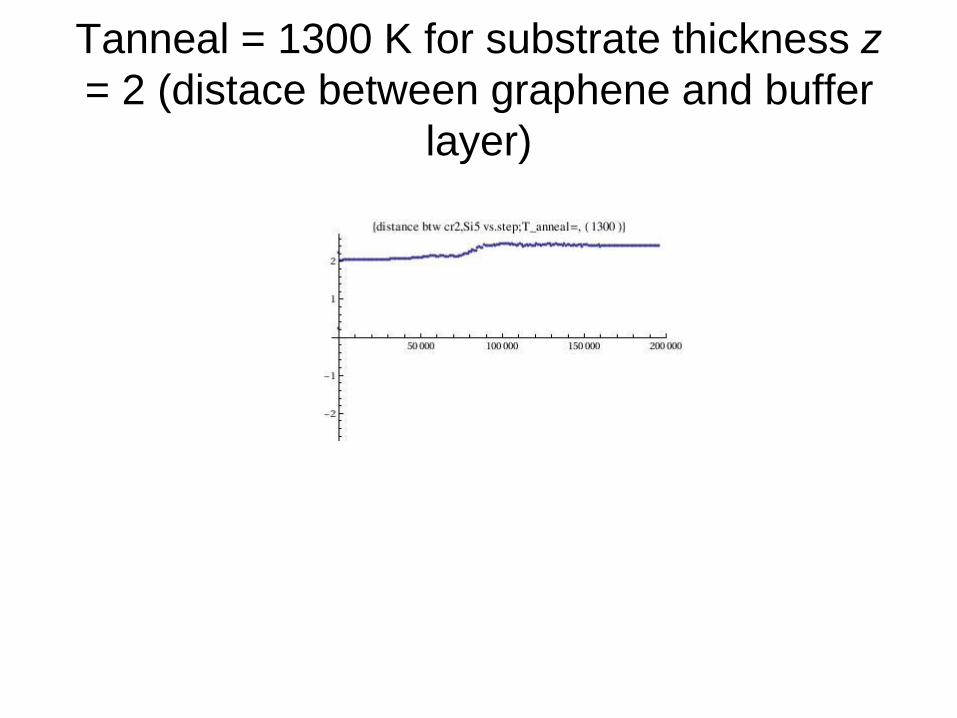
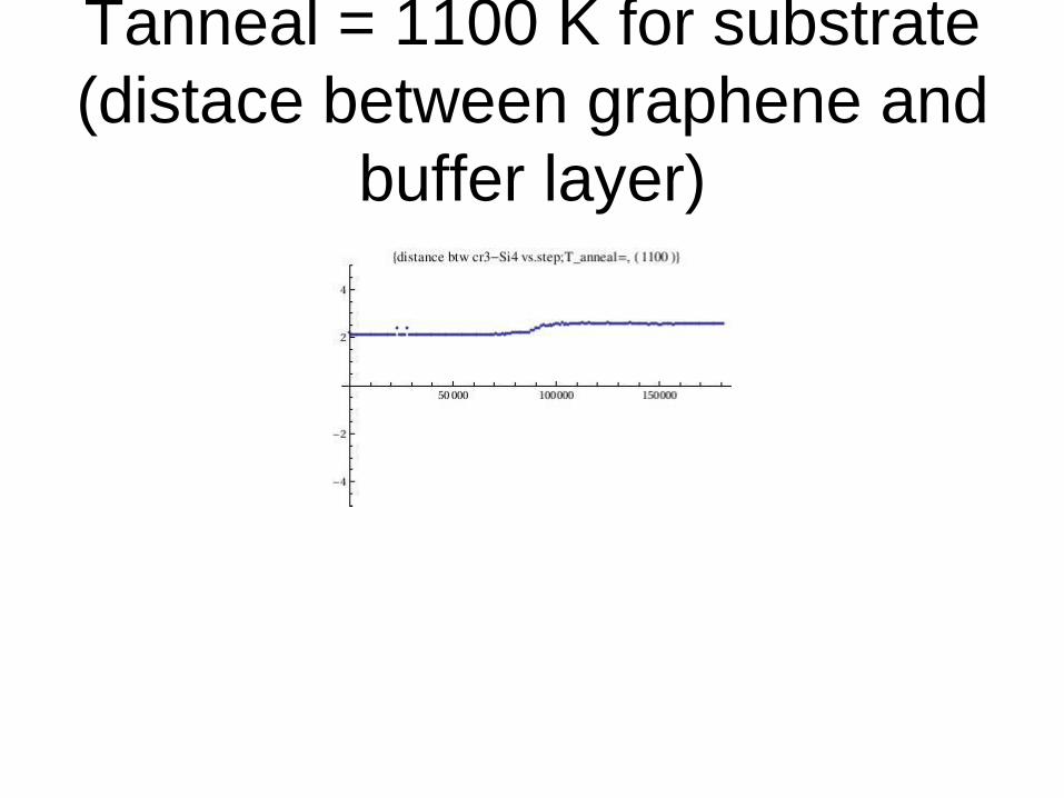
Tanneal = 700 K for substrate thickness z = 2
(distace between graphene and buffer layer)
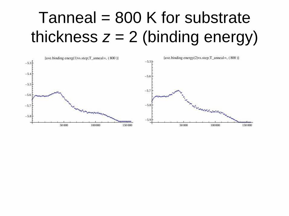
Tanneal = 800 K for substrate
thickness z = 2 (binding energy)
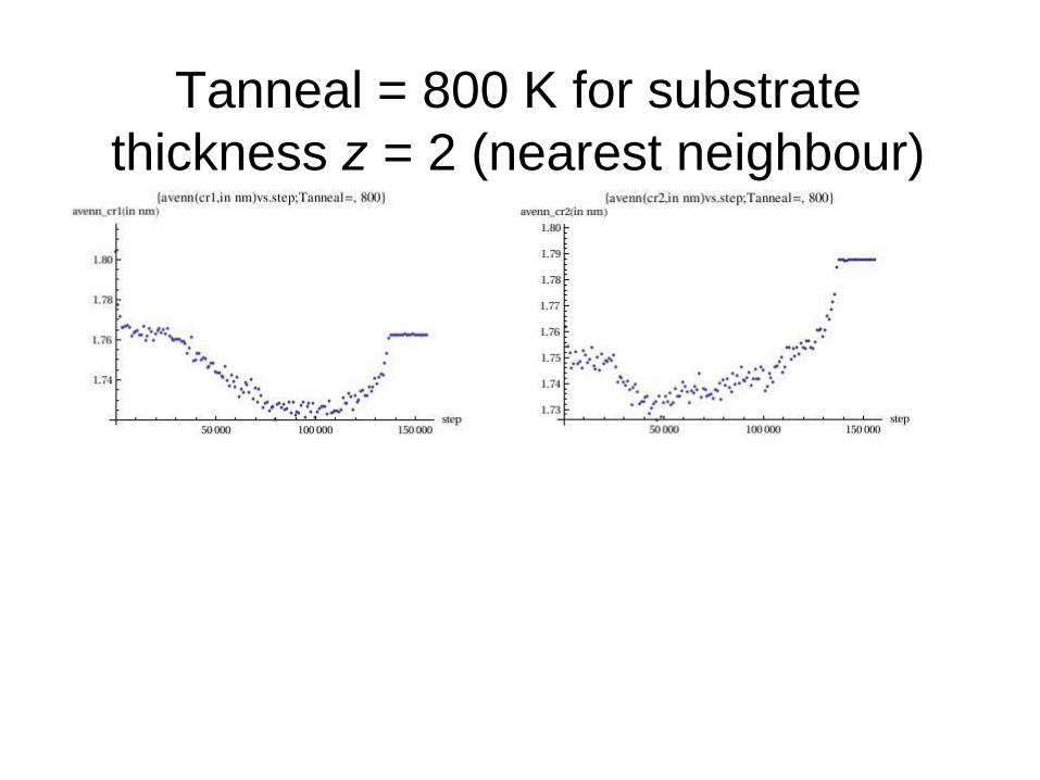
Tanneal = 800 K for substrate
thickness z = 2 (nearest neighbour)

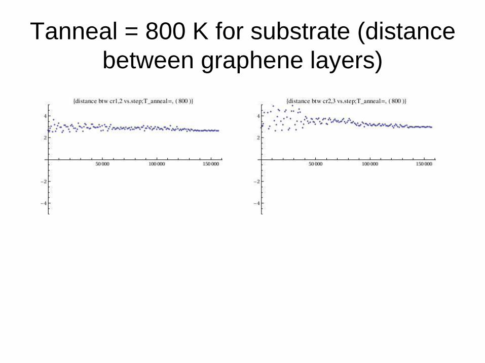
Tanneal = 800 K for substrate thickness z =
2 (distance between two graphene layer)
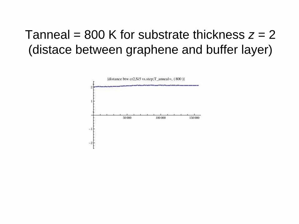
Tanneal = 800 K for substrate thickness z = 2
(distace between graphene and buffer layer)

Tanneal = 900 K for substrate
thickness z = 2 (binding energy)
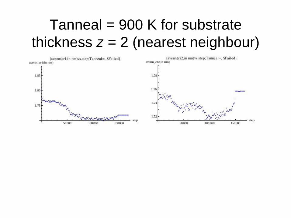
Tanneal = 900 K for substrate
thickness z = 2 (nearest neighbour)

Tanneal = 900 K for substrate thickness z =
2 (distance between two graphene layer)
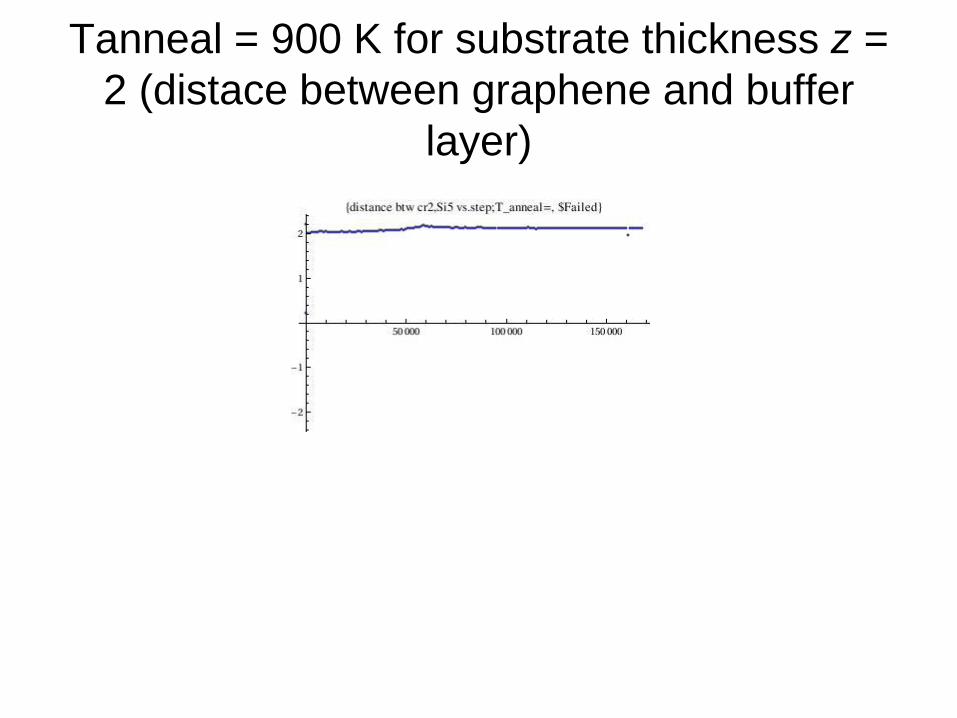
Tanneal = 900 K for substrate thickness z =
2 (distace between graphene and buffer
layer)
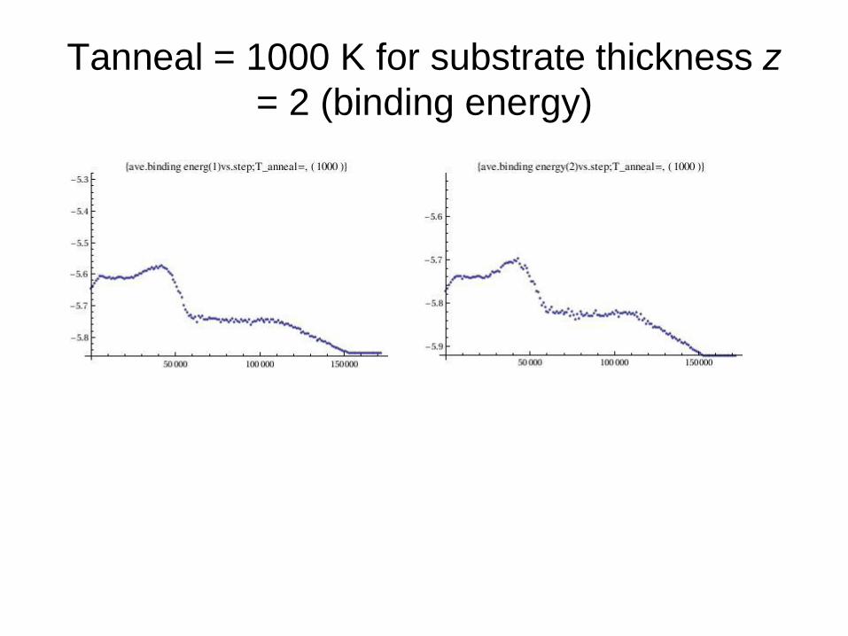
Tanneal = 1000 K for substrate thickness z
= 2 (binding energy)

Tanneal = 1000 K for substrate thickness z
= 2 (nearest neighbour)
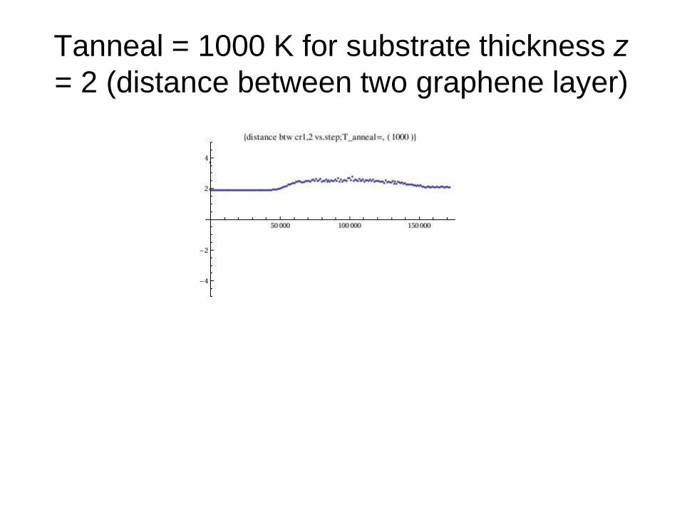
Tanneal = 1000 K for substrate thickness z
= 2 (distance between two graphene layer)

Tanneal = 1000 K for substrate thickness z
= 2 (distace between graphene and buffer
layer)
Tanneal = 1100 K for substrate thickness z
= 2 (binding energy)

Tanneal = 1100 K for substrate thickness z
= 2 (nearest neighbour)
Tanneal = 1100 K for substrate thickness z
= 2 (distance between two graphene layer)

Tanneal = 1100 K for substrate thickness z
= 2 (distace between graphene and buffer
layer)

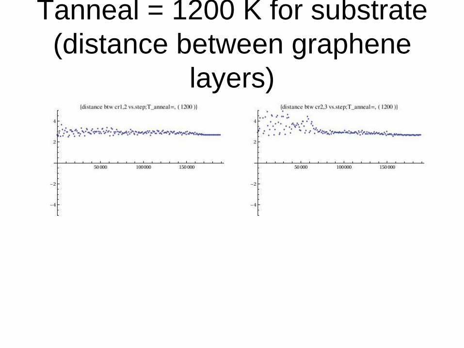
Tanneal = 1200 K for substrate thickness z
= 2 (binding energy)

Tanneal = 1200 K for substrate thickness z
= 2 (nearest neighbour)

Tanneal = 1200 K for substrate thickness z
= 2 (distance between two graphene layer)
Tanneal = 1200 K for substrate thickness z
= 2 (distace between graphene and buffer
layer)

Tanneal = 1300 K for substrate thickness z
= 2 (binding energy)
Tanneal = 1300 K for substrate thickness z
= 2 (nearest neighbour)

Tanneal = 1300 K for substrate thickness z
= 2 (distance between two graphene layer)
Tanneal = 1300 K for substrate thickness z
= 2 (distace between graphene and buffer
layer)
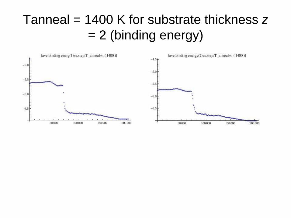
Tanneal = 1400 K for substrate thickness z
= 2 (binding energy)

Tanneal = 1400 K for substrate thickness z
= 2 (nearest neighbour)
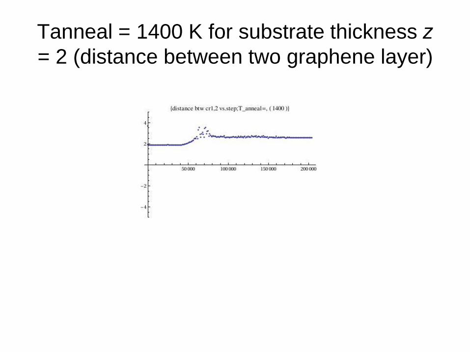
Tanneal = 1400 K for substrate thickness z
= 2 (distance between two graphene layer)

Tanneal = 1400 K for substrate thickness z
= 2 (distace between graphene and buffer
layer)
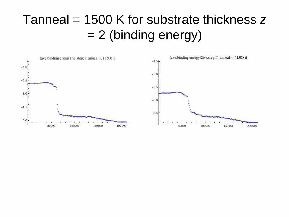
Tanneal = 1500 K for substrate thickness z
= 2 (binding energy)

Tanneal = 1500 K for substrate thickness z
= 2 (nearest neighbour)

Tanneal = 1500 K for substrate thickness z
= 2 (distance between two graphene layer)
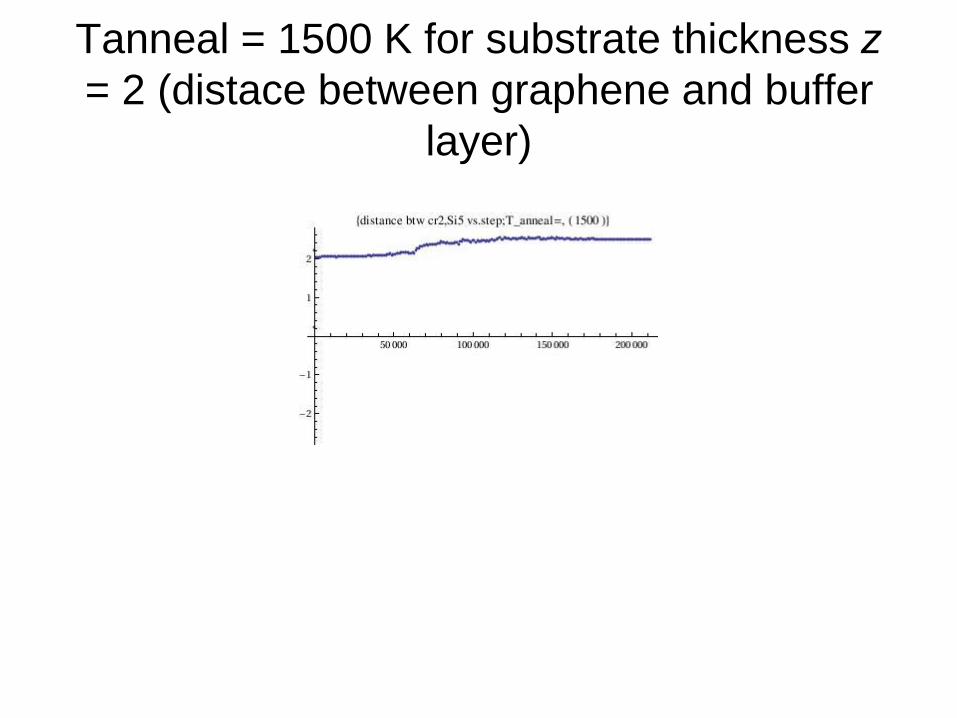
Tanneal = 1500 K for substrate thickness z
= 2 (distace between graphene and buffer
layer)
Summary of Annealing of 2
Layers Greaphene

Binding Energy
Top carbon-rich layer second carbon-rich
layer

Average Nearest Neighbour
Top carbon-rich layer second carbon-rich
layer
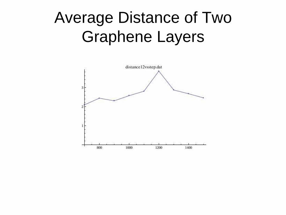
Average Distance of Two
Graphene Layers
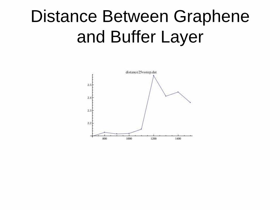
Distance Between Graphene
and Buffer Layer
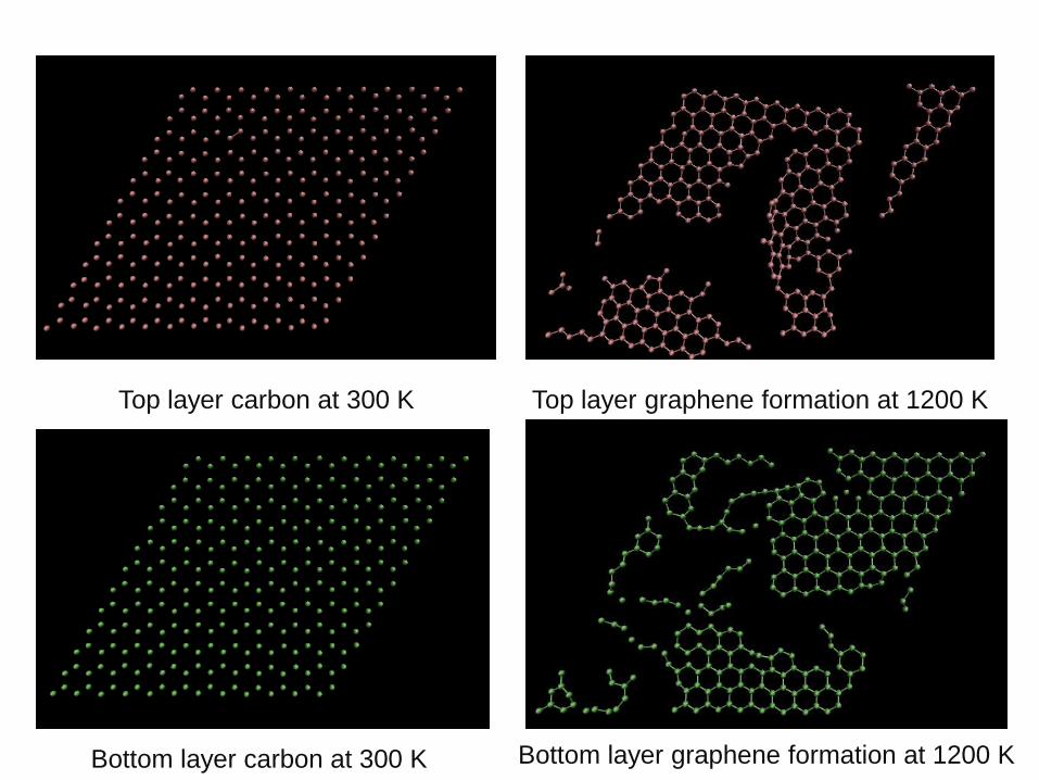
Top layer carbon at 300 K Top layer graphene formation at 1200 K
Bottom layer carbon at 300 K Bottom layer graphene formation at 1200 K
We have the identical results with the
thickness of substrate z=3
Three-layered carbon-rich
substrate with
thickness z = 2
for trilayered graphene
formation
117
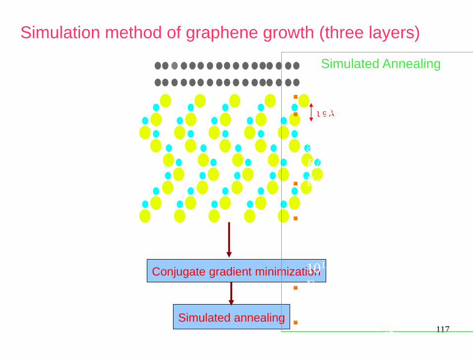
Simulation method of graphene growth (three layers)
1.9 Å
Conjugate gradient minimization
Simulated annealing
15
Simulated Annealing
Timestep = 0.5 fs
Increase the temperature
slowly until it attains 300 K
at approximately 5˟1013
K/s.
Equilibrating the system at
300 K for 20000 MD steps.
Raise the temperature of
the system slowly to the
desired T at approximately
1013 K/s.
Equilibrating the system at
T for 30000 MD steps.
Cool down the system until
0.1 K at 5x10¹² K/s
Extracting the result.

Simulated Annealing
Timestep = 0.5 fs
Increase the temperature slowly until it attains 300 K at
approximately 5˟1013 K/s.
Equilibrating the system at 300 K for 20000 MD steps.
Raise the temperature of the system slowly to the desired T at
approximately 1013 K/s.
Equilibrating the system at T for 30000 MD steps.
Cool down the system until 0.1 K at 5x10¹² K/s
Extracting the result.
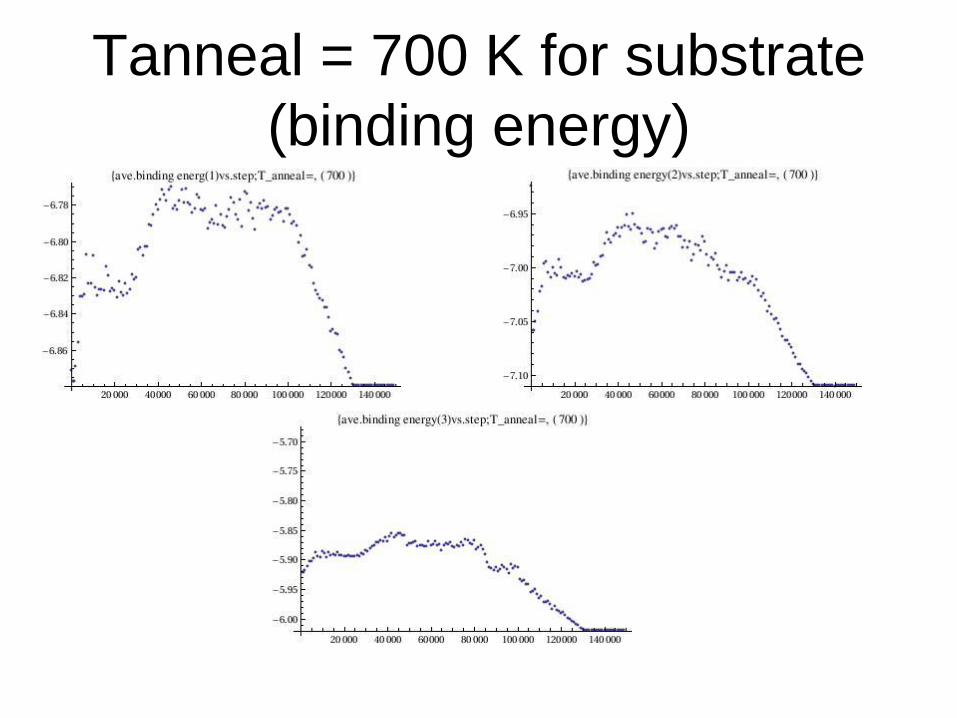
Tanneal = 700 K for substrate
(binding energy)

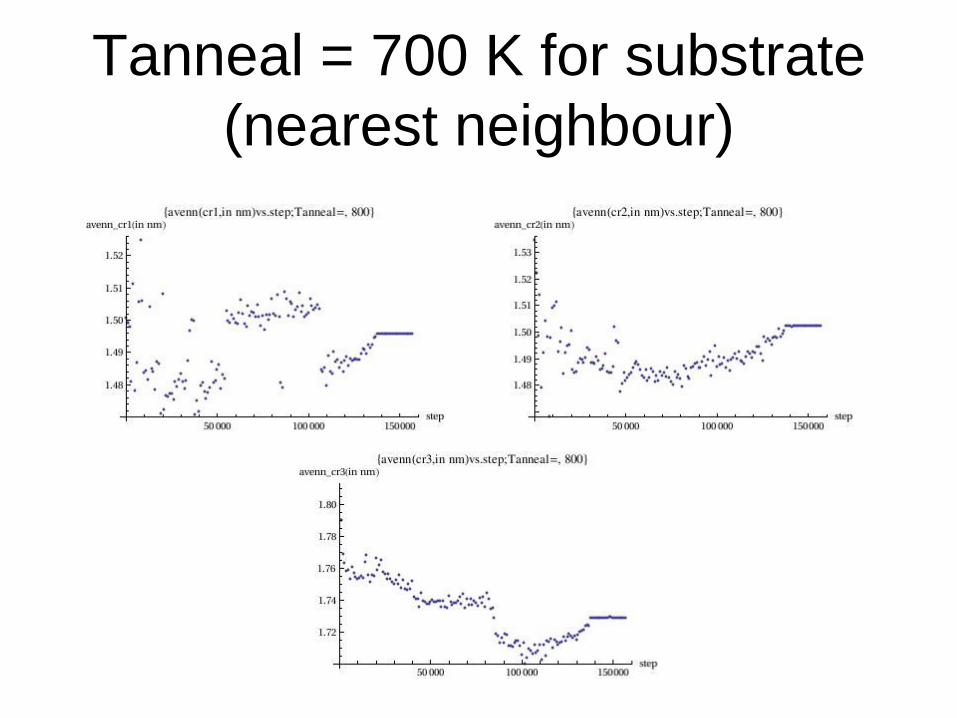
Tanneal = 700 K for substrate
(nearest neighbour)

Tanneal = 700 K for substrate (distance
between graphene layers)
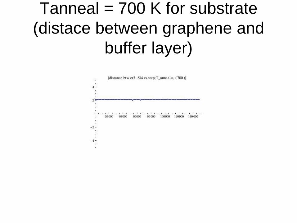
Tanneal = 700 K for substrate
(distace between graphene and
buffer layer)

Tanneal = 800 K for substrate
(binding energy)
Tanneal = 700 K for substrate
(nearest neighbour)
Tanneal = 800 K for substrate (distance
between graphene layers)

Tanneal = 800 K for substrate
(distace between graphene and
buffer layer)
Tanneal = 900 K for substrate
(binding energy)
Tanneal = 900 K for substrate
(nearest neighbour)
Tanneal = 900 K for substrate
(distance between graphene
layers)

Tanneal = 900 K for substrate
(distace between graphene and
buffer layer)
Tanneal = 1000 K for substrate
(binding energy)
Tanneal = 1000 K for substrate
(nearest neighbour)

Tanneal = 1000 K for substrate
(distance between graphene
layers)

Tanneal = 1000 K for substrate
(distace between graphene and
buffer layer)

Tanneal = 1100 K for substrate
(binding energy)

Tanneal = 1100 K for substrate
(nearest neighbour)
Tanneal = 1100 K for substrate
(distance between graphene
layers)
Tanneal = 1100 K for substrate
(distace between graphene and
buffer layer)

Tanneal = 1200 K for substrate
(binding energy)

Tanneal = 1200 K for substrate
(nearest neighbour)
Tanneal = 1200 K for substrate
(distance between graphene
layers)

Tanneal = 1200 K for substrate
(distace between graphene and
buffer layer)

Tanneal = 1300 K for substrate
(binding energy)
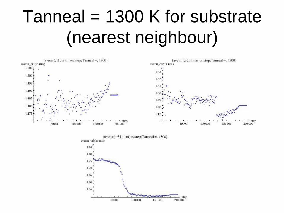
Tanneal = 1300 K for substrate
(nearest neighbour)

Tanneal = 1300 K for substrate
(distance between graphene
layers)
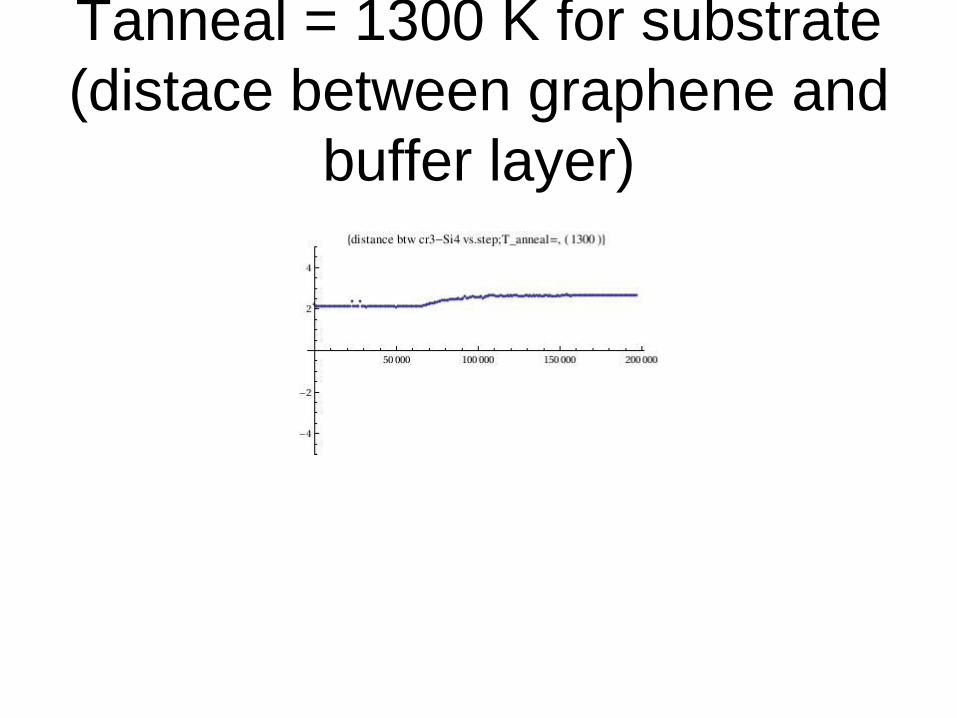
Tanneal = 1300 K for substrate
(distace between graphene and
buffer layer)
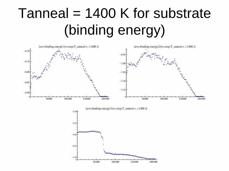
Tanneal = 1400 K for substrate
(binding energy)

Tanneal = 1400 K for substrate
(nearest neighbour)
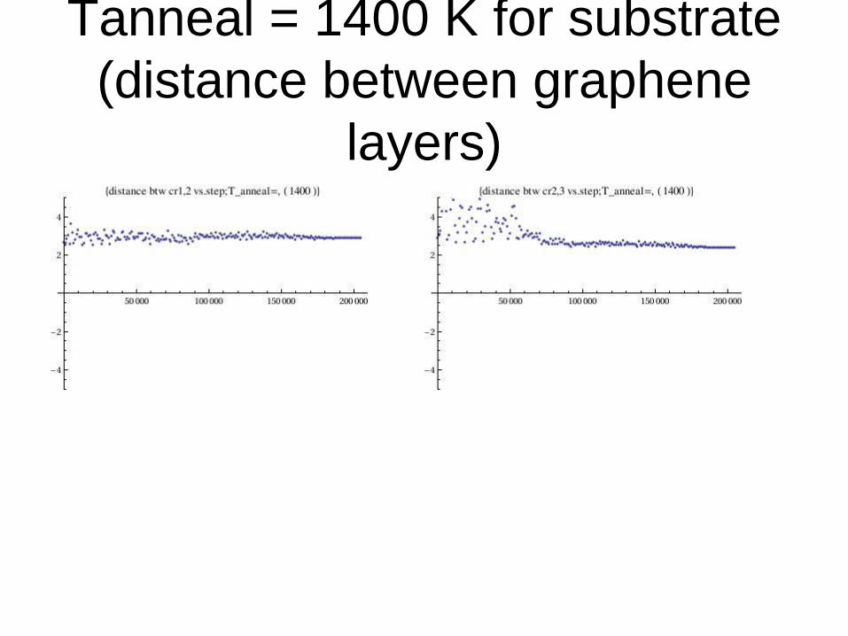
Tanneal = 1400 K for substrate
(distance between graphene
layers)

Tanneal = 1400 K for substrate
(distace between graphene and
buffer layer)

Tanneal = 1500 K for substrate
(binding energy)
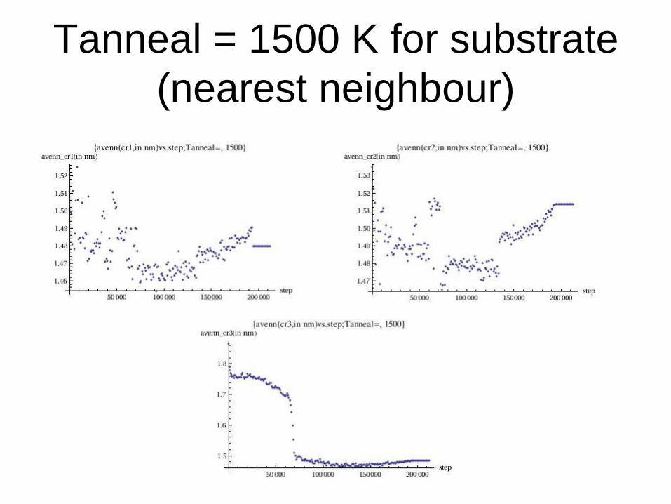
Tanneal = 1500 K for substrate
(nearest neighbour)
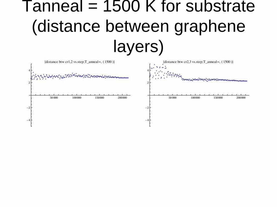
Tanneal = 1500 K for substrate
(distance between graphene
layers)

Tanneal = 1500 K for substrate
(distace between graphene and
buffer layer)
Summary

Binding Energy
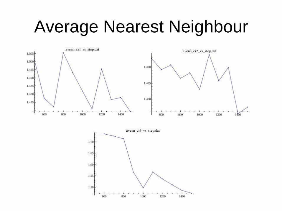
Average Nearest Neighbour
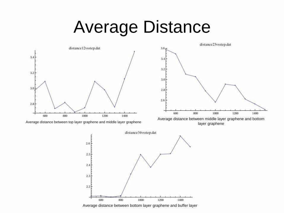
Average Distance
Average distance between top layer graphene and middle layer graphene Average distance between middle layer graphene and bottom
layer graphene
Average distance between bottom layer graphene and buffer layer

First layer graphene layer at 300K First layer graphenelayer at 1200K
Second layer graphene layer at 300K Second layer graphene layer at 1200K

Third layer graphene layer at 300K Third layer graphene layer at 1200K


