Page 1
MOLECULAR DYNAMICS SIMULATION OF
MONTMORILLONITE AND MECHANICAL AND
THERMODYNAMIC PROPERTIES CALCULATIONS
A Thesis
by
SELMA ATĐLHAN
Submitted to the Office of Graduate Studies of Texas A&M University
in partial fulfillment of the requirements for the degree of
MASTER OF SCIENCE
May 2007
Major Subject: Chemical Engineering
Page 2
MOLECULAR DYNAMICS SIMULATION OF
MONTMORILLONITE AND MECHANICAL AND
THERMODYNAMIC PROPERTIES CALCULATIONS
A Thesis
by
SELMA ATĐLHAN
Submitted to the Office of Graduate Studies of Texas A&M University
in partial fulfillment of the requirements for the degree of
MASTER OF SCIENCE
Approved by: Chair of Committee, Tahir Çağın Committee Members, Perla B. Balbuena Hung Jue Sue Head of Department, N.K. Anand
May 2007
Major Subject: Chemical Engineering
Page 3
iii
ABSTRACT
Molecular Dynamics Simulation of Montmorillonite and Mechanical and
Thermodynamic Properties Calculations. (May 2007)
Selma Atilhan, B.S., Ege University;
M.S., Ege University
Chair of Advisory Committee: Dr. Tahir Çağın
Nanocomposites refer to the materials in which the defining characteristic size of
inclusions is in the order of 10-100nm. There are several types of nanoparticle inclusions
with different structures: metal clusters, fullerenes particles and molybdenum selenide,
Our research focus is on polymer nanocomposites with inorganic clay particles as
inclusions, in particular we used sodium montmorillonite polymer nanocomposite.
In our study, modeling and simulations of sodium montmorillonite (Na+-MMT) is
currently being investigated as an inorganic nanocomposite material. Na+-MMT clay
consists of platelets, one nanometer thick with large lateral dimensions, which can be
used to achieve efficient reinforcement of polymer matrices. This nanocomposite has
different applications such as a binder of animal feed, a plasticizing agent in cement,
brick and ceramic, and a thickener and stabilizer of latex and rubber adhesives.
In this study, sodium montmorillonite called Na+-MMT structure is built with the
bulk system and the layered system which includes from 1 to 12 layers by using Crystal
Builder of Cerius2. An isothermal and isobaric ensemble is used for calculation of
thermodynamic properties such as specific heat capacities and isothermal expansion
coefficients of Na+-MMT. A canonical ensemble which holds a fixed temperature,
volume and number of molecules is used for defining exfoliation kinetics of layered
structures and surface formation energies for Na+-MMT layered structures are calculated
by using a canonical ensemble. Mechanical properties are used to help characterize and
identify the Na+-MMT structure. Several elastic properties such as compliance and
stiffness matrices, Young's, shear, and bulk modulus, volume compressibility, Poisson's
ratios, Lamé constants, and velocities of sound are calculated in specified directions.
Page 4
iv
Another calculation method is the Vienna Ab-initio Simulation Package (VASP). VASP
is a complex package for performing ab-initio quantum-mechanical calculations and
molecular dynamic (MD) simulations using pseudopotentials and a plane wave basis set.
Cut off energy is optimized for the unit cell of Na+-MMT by using different cut off
energy values. Experimental and theoretical cell parameters are compared by using cell
shape and volume optimization and root mean square (RMS) coordinate difference is
calculated for variation of cell parameters. Cell shape and volume optimization are done
for calculating optimum expansion or compression constant.
Page 5
v
DEDICATION
To my excellent husband, Mert and our families
Page 6
vi
ACKNOWLEDGMENTS
I can hardly thank my advisor and the committee chair Dr. Çağın enough. He truly
has been my role model and guided me in the right track of research and life too. I
sincerely thank my committee members, Perla B. Balbuena and Hung Jue Sue, for
serving on my committee.
I would like to express my appreciation to my group members, especially Mustafa
Uludoğan, Arnab Chakrabarty and Oscar Ojeda, for valuable discussions, exchange of
ideas and friendship.
I’ve been delighted to have such wonderful professors, colleagues, and friends here in
College Station. Mr.Polasek’s help regarding computer issues was truly invaluable.
Finally, I am forever grateful for the love and support of my parents and my husband.
As teachers, my mother and father taught me the value of education. As parents, they
instilled in me the importance of doing my best regardless of the circumstances. I am
blessed to have them as parents and honored to have them as my role models. I want to
thank my parents-in-law for their support and for giving their best wishes to us. Also I
want to express my appreciation to my sister, brother, brothers-in-law and sisters-in-law
for their support. Above all, I am indebted to my husband Mert for his love, support,
encouragement, advice in hard times, and moreover, for the many sacrifices he made for
the pursuit of my career ambitions. He truly is my foundation.
Page 7
vii
NOMENCLATURE
α: Lattice angle between x and y directions
β: Lattice angle between x and z directions
γ : Lattice angle between y and z directions
a: Lattice parameter
b: Lattice parameter
c: Lattice parameter
ξ: Atomic position on x direction
µ: Atomic position on y direction
ς: Atomic position on z direction
Page 8
viii
TABLE OF CONTENTS
Page
ABSTRACT ............................................................................................................... iii
DEDICATION..............................................................................................................v
ACKNOWLEDGMENTS .......................................................................................... vi
NOMENCLATURE .................................................................................................. vii
TABLE OF CONTENTS ......................................................................................... viii
LIST OF FIGURES ..................................................................................................... x
LIST OF TABLES....................................................................................................... x
CHAPTER
I INTRODUCTION..................................................................................................1
1.1 Definition of Nanocomposites.......................................................................1 1.2 Structure and Chemical Formula of Clay ......................................................2 1.3 Montmorillonite.............................................................................................3
1.3.1 Montmorillonite and Its Physical Properties ....................................3 1.3.2 Sodium Montmorillonite and Its Applications .................................4
1.4 Synthetic Methods for Polymer Layered Clay Nanocomposites...................5
II THEORY .............................................................................................................9
2.1 Introduction to Molecular Simulation ...........................................................9 2.2 Molecular Dynamics....................................................................................10
2.2.1 Force Fields.....................................................................................12 2.2.1.1 The Energy Expression ............................................................13 2.2.1.2 Advantages of Having Several Force Fields............................13 2.2.1.3 Types of Force Field ................................................................14
2.2.1.3.1 Dreiding Force Field...........................................................16 2.2.1.3.2 Morse Charge Equilibration (MS-Q) Force Field...............21
2.2.2 Ensembles .......................................................................................22 2.2.3 Types of Molecular Dynamics........................................................23
2.3 Ab-Initio ......................................................................................................25 2.3.1 Density Functional Theory .............................................................25 2.3.2 Advantages and Limitations of Ab-Initio Calculations ..................29
Page 9
ix
CHAPTER ....................................................................................................................Page
2.4 Properties from Simulation ...........................................................................30 2.5 A Survey of Earlier Work on Clay-Polymer Composites Literature Survey
III RESULTS AND DISCUSSIONS.....................................................................36
3.1 Computational Details...................................................................................36 3.1.1 Interaction Force Field: Functional Forms and Parameters Used
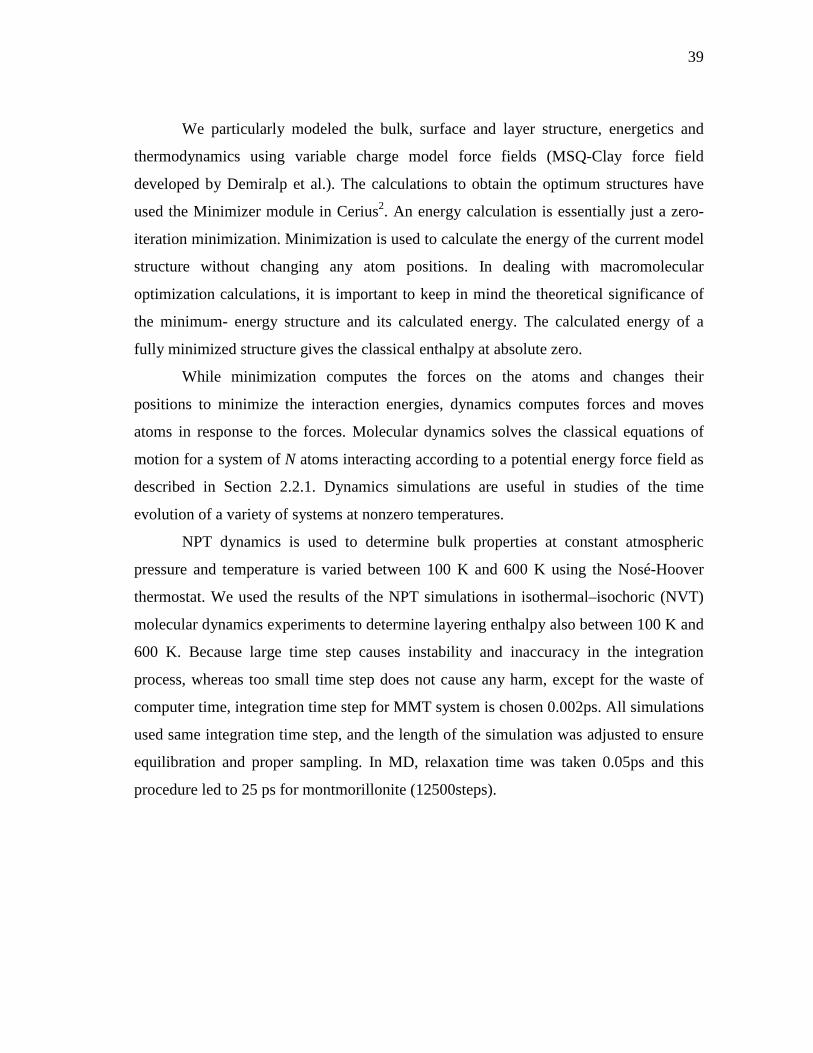
In Simulations ................................................................................36 3.1.2 Model Construction and Molecular Dynamics of MMT.................38
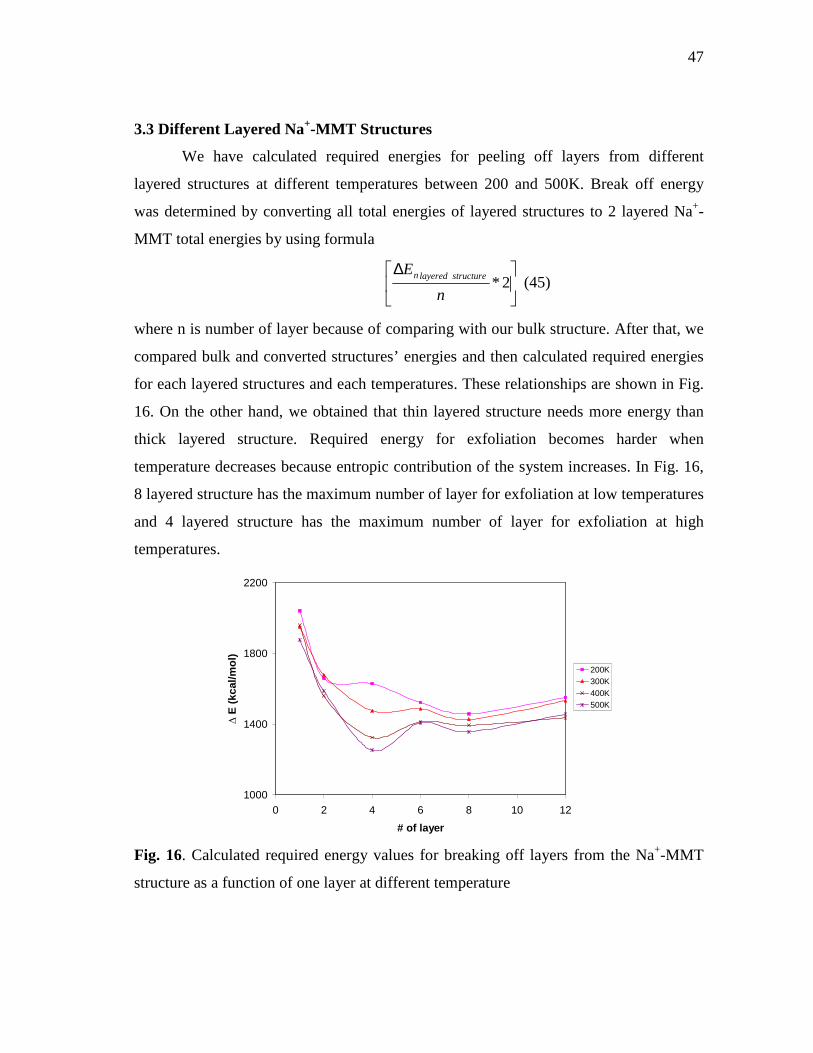
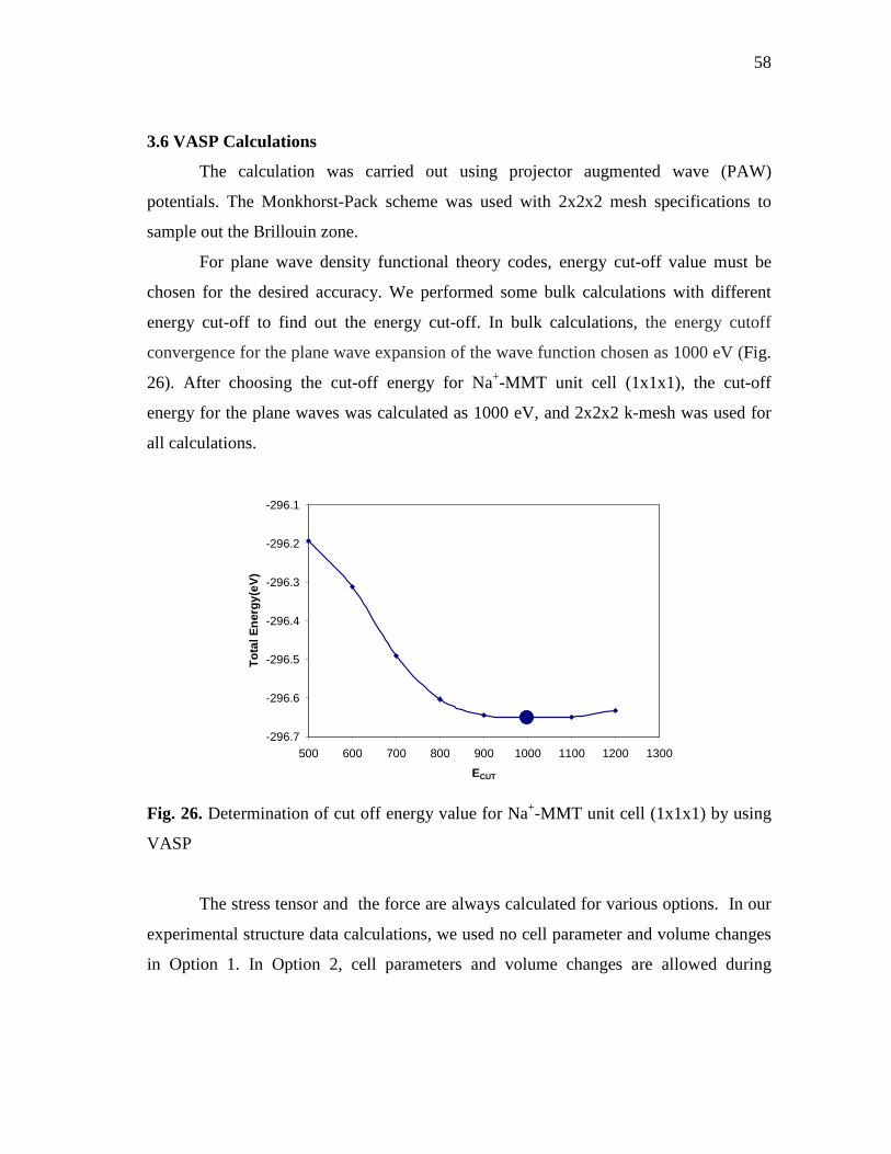
3.2 Na+-MMT Bulk Structure (3x2x2) by Using NPT Molecular Dynamics.....42 3.3 Different Layered Na+-MMT Structures.......................................................47 3.4 Na+-MMT Unit Cell (1x1x1) by Using NVT Molecular Dynamics...........50 3.5 Exfoliation Studies on Organically Modified-MMT....................................56 3.6 VASP Calculations .......................................................................................58
IV CONCLUSION ..............................................................................................62
REFERENCES ...........................................................................................................64
APPENDIX A.............................................................................................................69
APPENDIX B.............................................................................................................71
VITA...........................................................................................................................81
34
Page 10
x
LIST OF FIGURES
Page
Fig. 1. Structure of 2:1 phyllosilicates [3] ..........................................................................2 Fig. 2. Polyhedra rendering of crystal structure of Na+-montmorillonite clay ..................3 Fig. 3. Schematic view of preparation methods for polymer intercalation
compounds [7] ........................................................................................................7 Fig. 4. Scheme of different types of composite arising from the interaction of
polymers and layered nanocomposites[12].............................................................8 Fig. 5. Dreiding FF bonded and nonbonded interactions..................................................18 Fig. 6. Schematic illustration of the self-consist cycles in ab initio
calculations ...........................................................................................................28 Fig. 7. Na+-MMT bulk structure .......................................................................................41 Fig. 8. MMT-NH3CH3 ......................................................................................................41 Fig. 9. Models of layered structures of Na+-MMT ...........................................................41 Fig. 10. Total energy changes with respect to temperature for Na+-MMT bulk
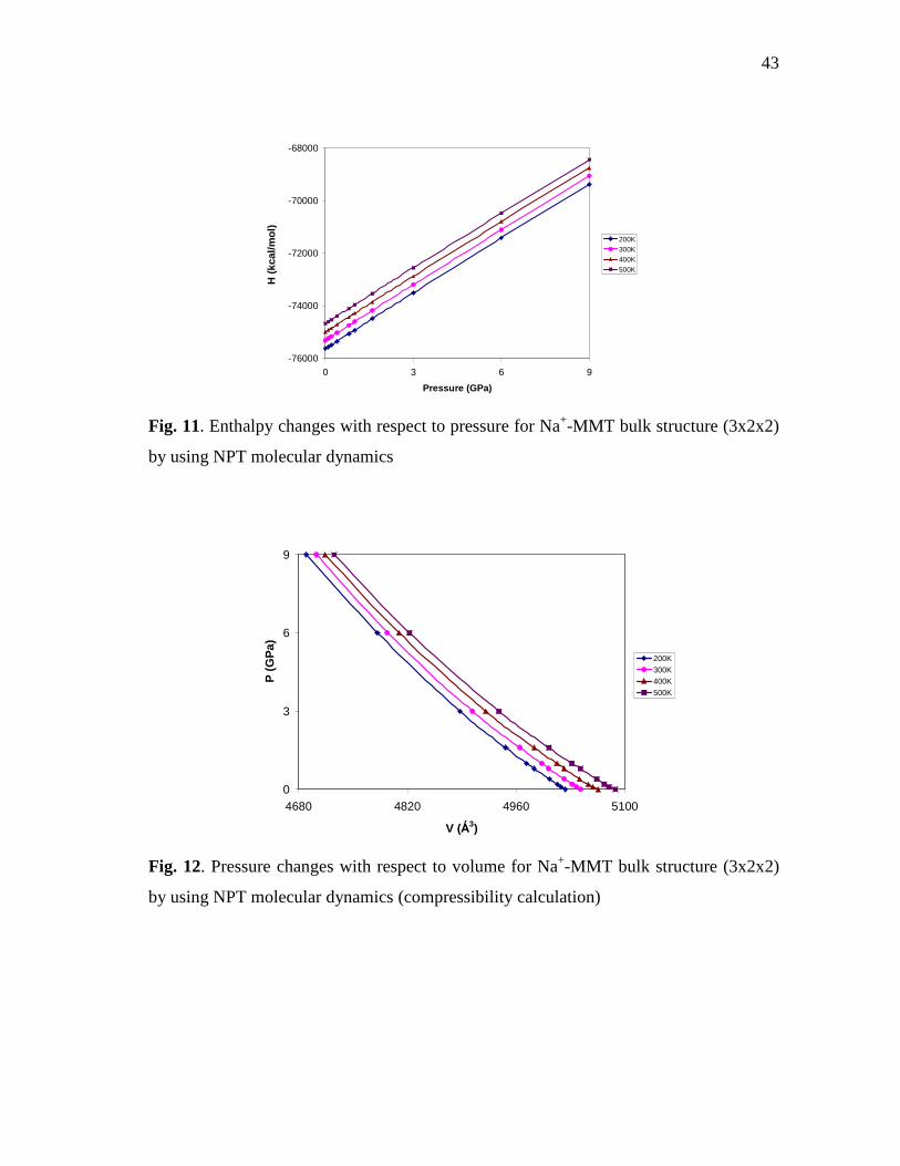
structure (3x2x2) by using NPT molecular dynamics ..........................................42 Fig. 11. Enthalpy changes with respect to pressure for Na+-MMT bulk
structure (3x2x2) by using NPT molecular dynamics ..........................................43 Fig. 12. Pressure changes with respect to volume for Na+-MMT bulk
structure (3x2x2) by using NPT molecular dynamics (compressibility calculation)............................................................................................................43
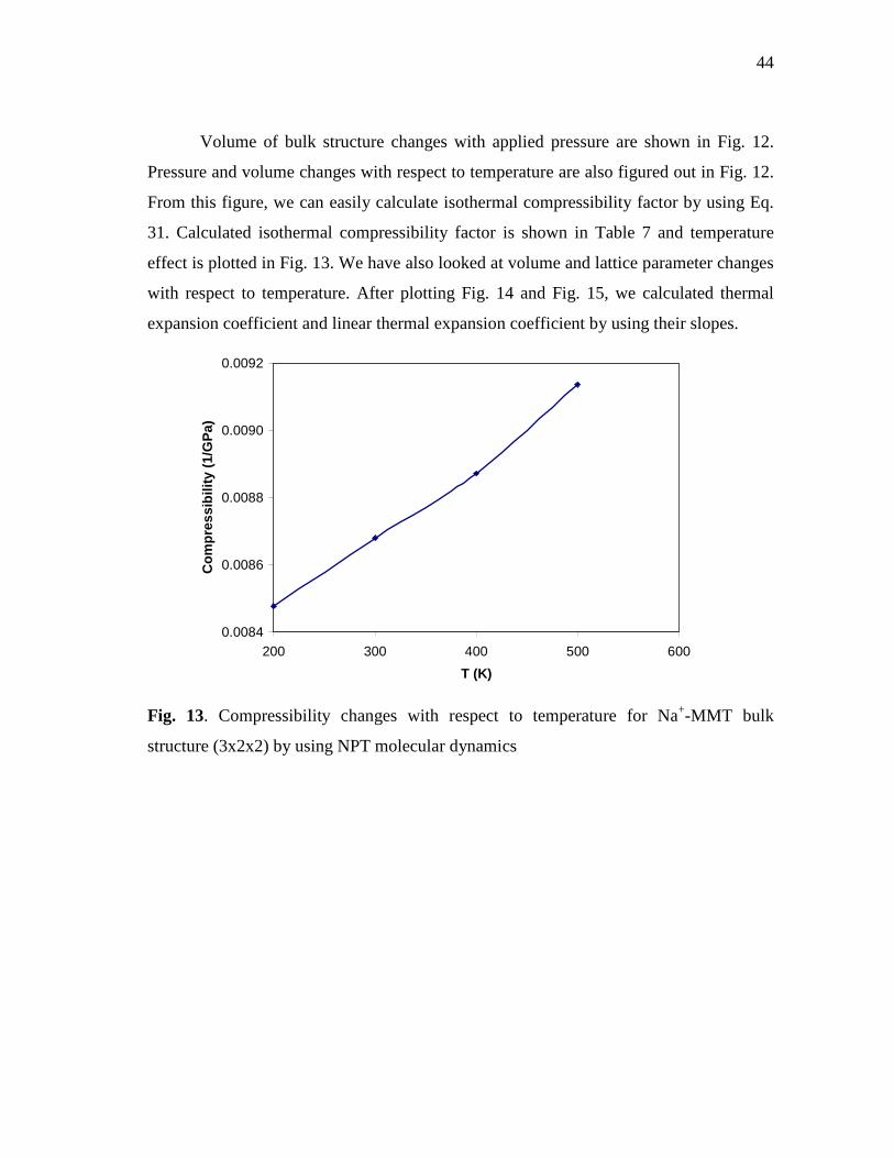
Fig. 13. Compressibility changes with respect to temperature for Na+-MMT
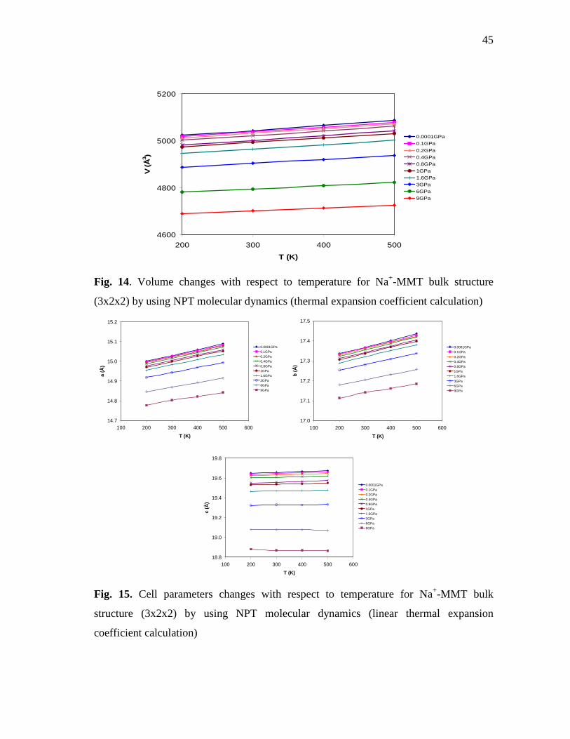
bulk structure (3x2x2) by using NPT molecular dynamics ..................................44 Fig. 14. Volume changes with respect to temperature for Na+-MMT bulk
structure (3x2x2) by using NPT molecular dynamics (thermal expansion coefficient calculation) ........................................................................45
Fig. 15. Cell parameters changes with respect to temperature for Na+-MMT
bulk structure (3x2x2) by using NPT molecular dynamics (linear thermal expansion coefficient calculation) ...........................................................45
Page 11
xi
Page Fig. 16. Calculated required energy values for breaking off layers from the
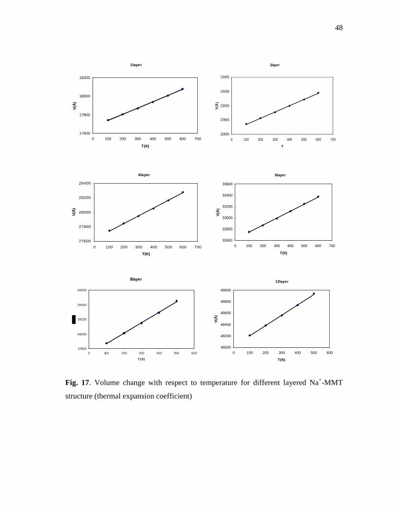
Na+-MMT structure as a function of one layer at different temperature ..............47 Fig. 17. Volume change with respect to temperature for different layered
Na+-MMT structure (thermal expansion coefficient) ...........................................48 Fig. 18. Total energy changes with respect to temperature for different
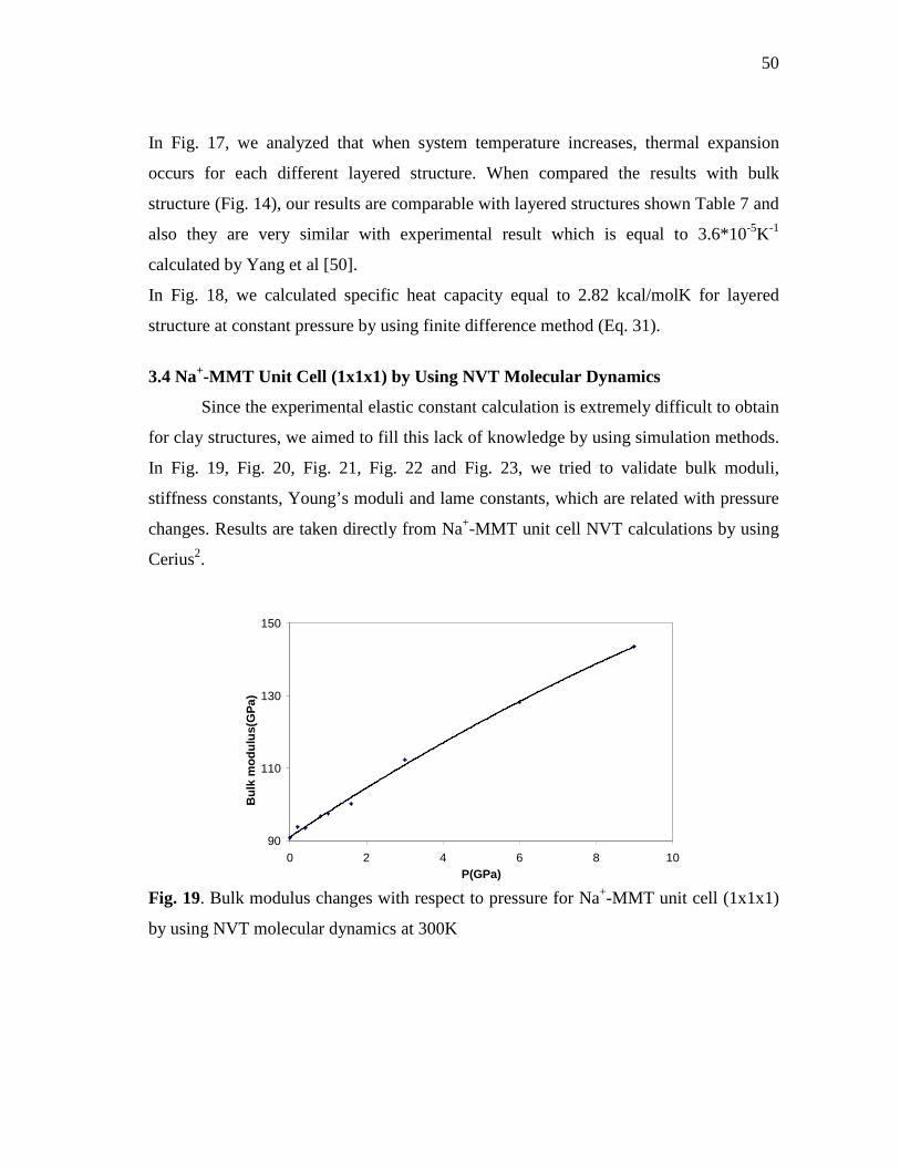
layered Na+-MMT structure (Cp calculation).......................................................49 Fig. 19. Bulk modulus changes with respect to pressure for Na+-MMT unit
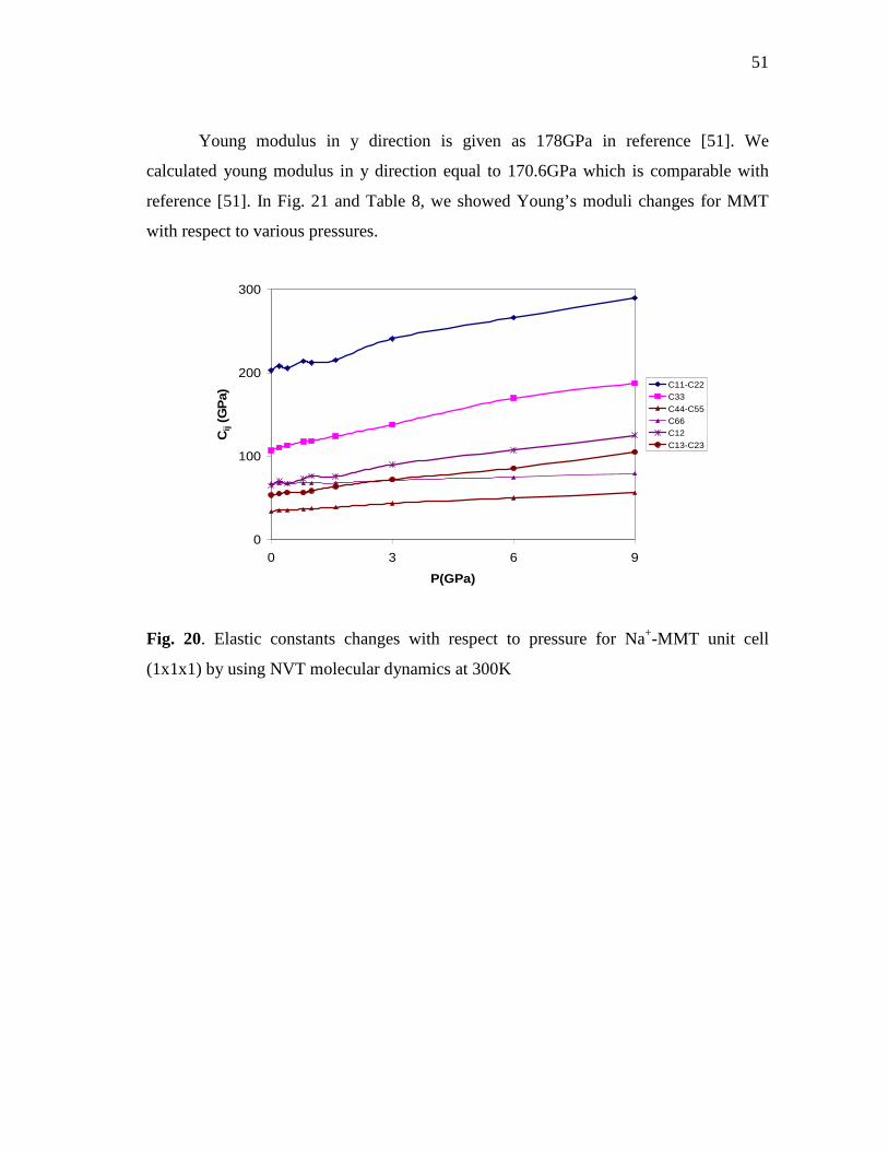
cell (1x1x1) by using NVT molecular dynamics at 300K ....................................50 Fig. 20. Elastic constants changes with respect to pressure for Na+-MMT unit
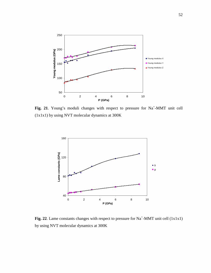
cell (1x1x1) by using NVT molecular dynamics at 300K ....................................51 Fig. 21. Young’s moduli changes with respect to pressure for Na+-MMT unit
cell (1x1x1) by using NVT molecular dynamics at 300K ....................................52 Fig. 22. Lame constants changes with respect to pressure for Na+-MMT unit
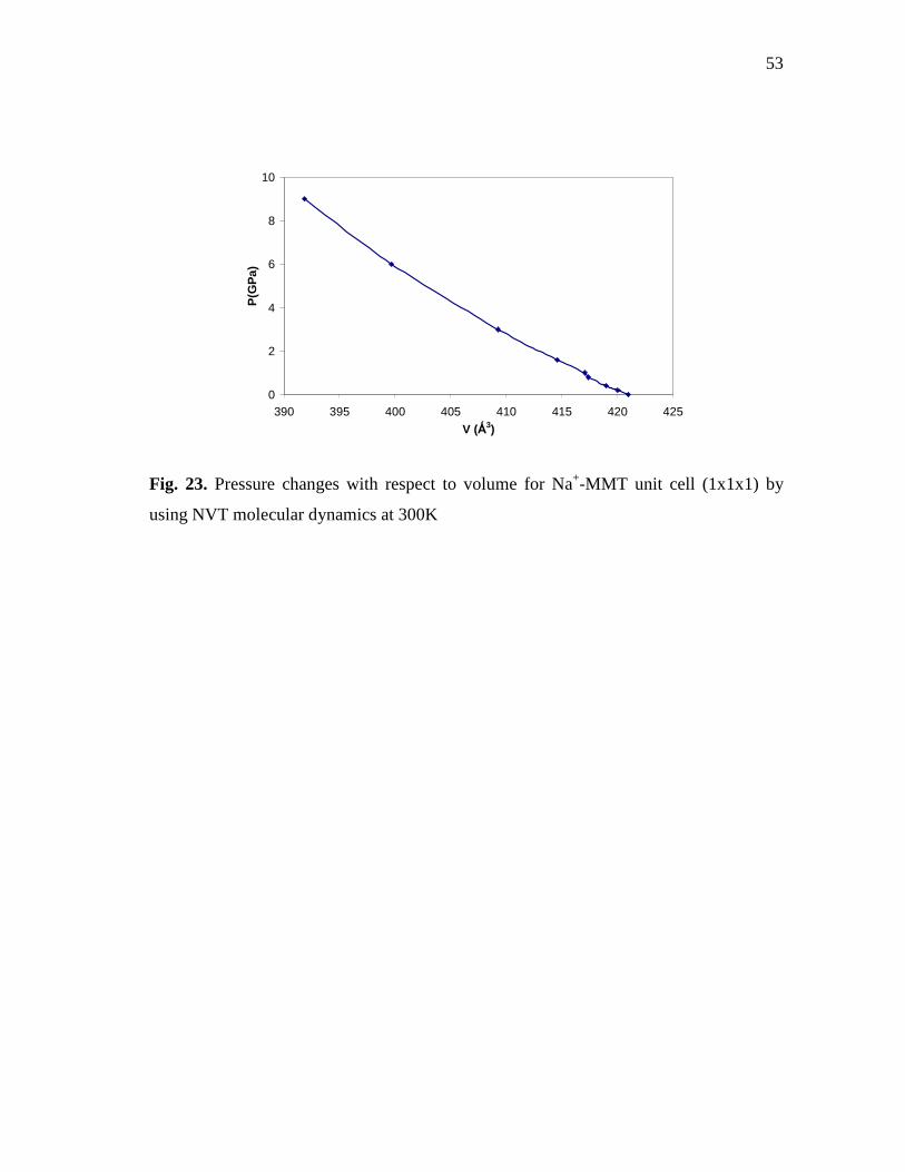
cell (1x1x1) by using NVT molecular dynamics at 300K ....................................52 Fig. 23. Pressure changes with respect to volume for Na+-MMT unit cell
(1x1x1) by using NVT molecular dynamics at 300K...........................................53 Fig. 24. Annealing procedure for alkyl amine-MMT molecular dynamics......................56 Fig. 25. Gallery height versus number of carbons n in the AA tail average at
3000C.....................................................................................................................57 Fig. 26. Determination of cut off energy value for Na+-MMT unit cell
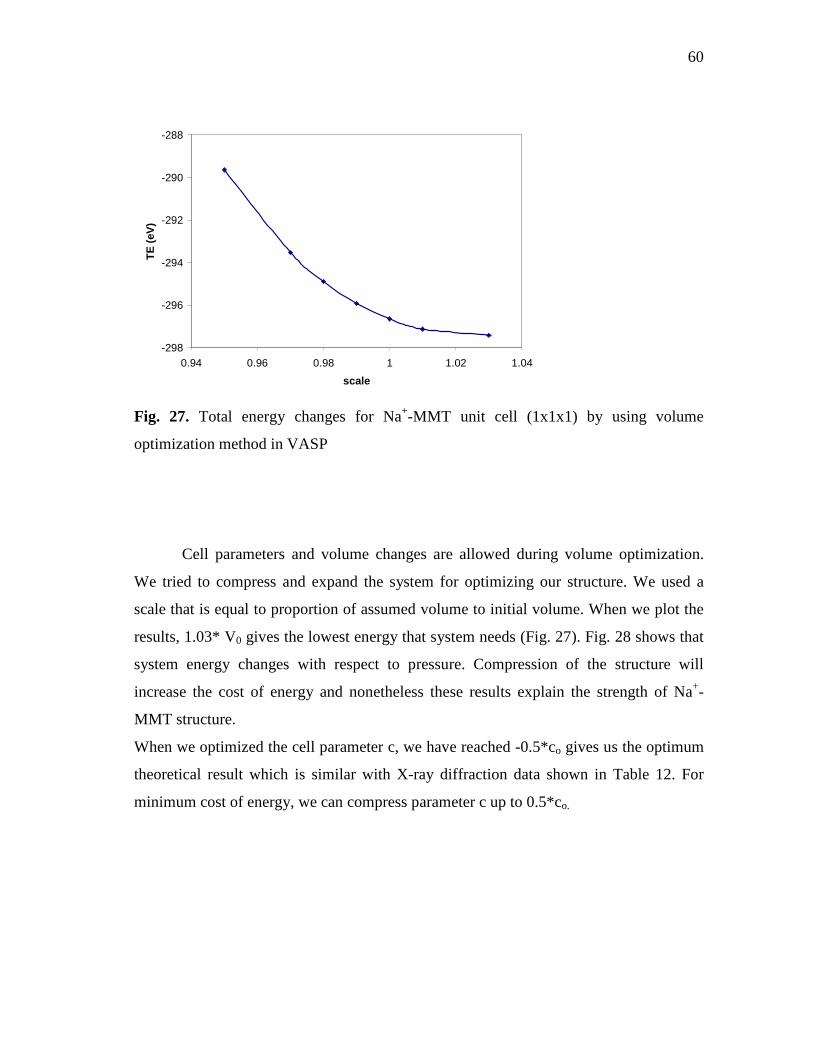
(1x1x1) by using VASP........................................................................................58 Fig. 27. Total energy changes for Na+-MMT unit cell (1x1x1) by using
volume optimization method in VASP.................................................................60 Fig. 28. Pressure and total energy changes for Na+-MMT unit cell (1x1x1)
during volume optimization in VASP...................................................................61
Page 12
xii
LIST OF TABLES
Page
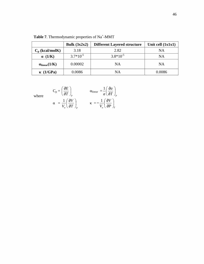
Table 1. Montmorillonite clay properties ...........................................................................4 Table 2. Types of ensembles.............................................................................................24 Table 3. Diagonal Morse type Van der Waals potential...................................................37 Table 4. Off-diagonal Morse type Van der Waals potential .............................................38 Table 5. Lattice parameters of Na-montmorillonite [49]..................................................38 Table 6. Na+-montmorillonite atomic coordinates [48, 49]..............................................40 Table 7. Thermodynamic properties of Na+-MMT...........................................................46 Table 8. Mechanical properties calculated by using Cerius2 of Na+-MMT
unit cell (1x1x1) at 300K ......................................................................................55 Table 9. Mechanical properties calculated by using Cerius2 of Na+-MMT
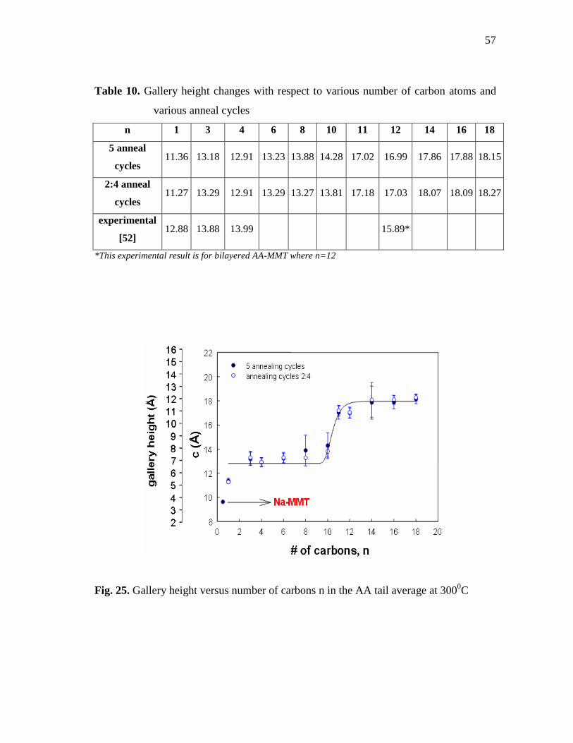
unit cell (1x1x1) at 300K (continued) ..................................................................56 Table 10. Gallery height changes with respect to various number of carbon
atoms and various anneal cycles ...........................................................................57 Table 11. Na+-MMT unit cell shape and volume optimization ........................................59 Table 12. Optimization of cell parameter c and RMS results for Na+-MMT
unit cell (1x1x1) by using volume optimization method in VASP.......................61
Page 13
1
CHAPTER I
INTRODUCTION
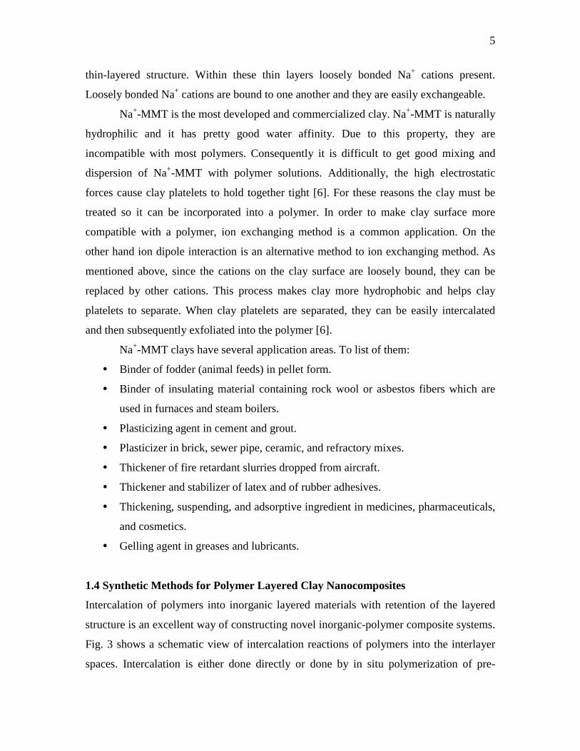
1.1 Definition of Nanocomposites
The material systems described as nanocomposites getting richer day by day over
a range of systems with one, two and three dimensional nanoscale composites in various
matrix materials such as metals, ceramics and polymers.
Inorganic-polymer nanocomposites are composites with inorganic materials as
inclusions. The inorganic components can be a three-dimensional framework systems
such as feldspar group (albite, microcline), feldspathoid group (cancrinite, leucite,
sodalite), quartz group (coesite, quartz, tridymite) and zeolite group (analcime, mesolite,
phillipsite), two-dimensional layered materials such as clays (kaolinite,
montmorillonite/smectite, clay-mica and chlorite groups), metal oxides (V2O5 xerogel
and aerogel), silicates (aluminum silicates, magnesium silicates, magnesium iron
silicates, zirconium silicates, potassium magnesium aluminum silicate hydroxide
fluorides), n-silicates, metal phosphates, and even one-dimensional such as nanowire,
nanorod, nanotube and zero-dimensional materials such as (Mo3Se3)-, fullerene particles
and clusters. Experiments indicate that essentially all types and classes of nanocomposite
materials lead to new and enhanced properties when compared to their macrocomposite
analogues. Consequently, nanocomposites have potential new applications in several
areas such as mechanically reinforced light-weight components (Concrete, Carbon-fiber-
reinforced plastics), non-linear optics (metal and semiconductor nanocomposites (copper,
silver nanoparticles, β-BaB2O4, LiB3O5)), nanosensors (chemical nanosensors used on
multi wall carbon nanotubes, devices and methods for detection of basic gases and
thermal nanosensors used for temperature control, fire detection, engine environment
monitoring (coolant and lubricant temperatures)), battery cathodes (V2O5, V6O13),
nanowires.
This thesis follows the style of Materials Science and Engineering: R: Reports.
Page 14
2
1.2 Structure and Chemical Formula of Clay
Clay is a natural, earthy, fine-grained material that develops plasticity when
mixed with a limited amount of water. The most common clay minerals can be classified
into five groups: smectite (montmorillonite, beidellite); illite (illite and glauconite);
kaolinite (kaolinite, halloysite); chlorite (chlorite); sepolite (sepolite and palygorskite)
[1].
Structurally, clays are built up of layers of octahedral and tetrahedral sheets. The
primary building blocks of these sheets are the aluminum octahedron and the silica
tetrahedron. The Al3+ is generally found in six fold or octahedral coordination while the
Si4+ cation takes place in four fold or tetrahedral coordination with oxygen [1]. Layered
silicates is a member of the 2:1 phyllosilicates structural family, in which the central
octahedral alumina sheet is sandwiched between two tetrahedral silica sheets [2] (Fig. 1).
These layered crystals, which are approximately 1nm thick with lateral dimensions from
30nm to several microns, are piled parallel to each other and are bonded by local van der
Walls and electrostatic forces.
Fig. 1. Structure of 2:1 phyllosilicates [3]
Clays are naturally occurring minerals; they must be purified before use. The
most commonly encountered layered silicates are montmorillonite, hectorite and
saponite. The clay layers allow delocalization of negative charges. These negative
charges are then neutralized by cations such as H+, Na+, K+, Mg2+ or Ca2+ situated in
Page 15
3
between the charged layers. Because of their high hydrophilic nature, water molecules
generally position between the clay layers [1, 2] as well.
1.3 Montmorillonite
1.3.1 Montmorillonite and Its Physical Properties
Montmorillonite (MMT) is a well known clay mineral. The name derives from the
French town Montmorillon, where it was discovered by Damour and Salvetat in 1847.
MMT is formed by weathering of eruptive rock material (usually tuffs and volcanic ash).
In its pure form, MMT includes trace amounts of crystobalite, zeolites, biotite, quartz,
feldspar, zirconia, as well as some other minerals found in volcanic rocks [1]. MMT has a
crystallographic structure based on pyrophyllite model. Pyrophyllite model structure
consists of two silica tetrahedral sheets sandwiching an edge-shared octahedral sheet of
either aluminum or magnesium hydroxide, known as t-o-t sheets. A polyhedra
representation of MMT crystal structure is given in Fig. 2.
Fig. 2. Polyhedra rendering of crystal structure of Na+-montmorillonite clay
Page 16
4
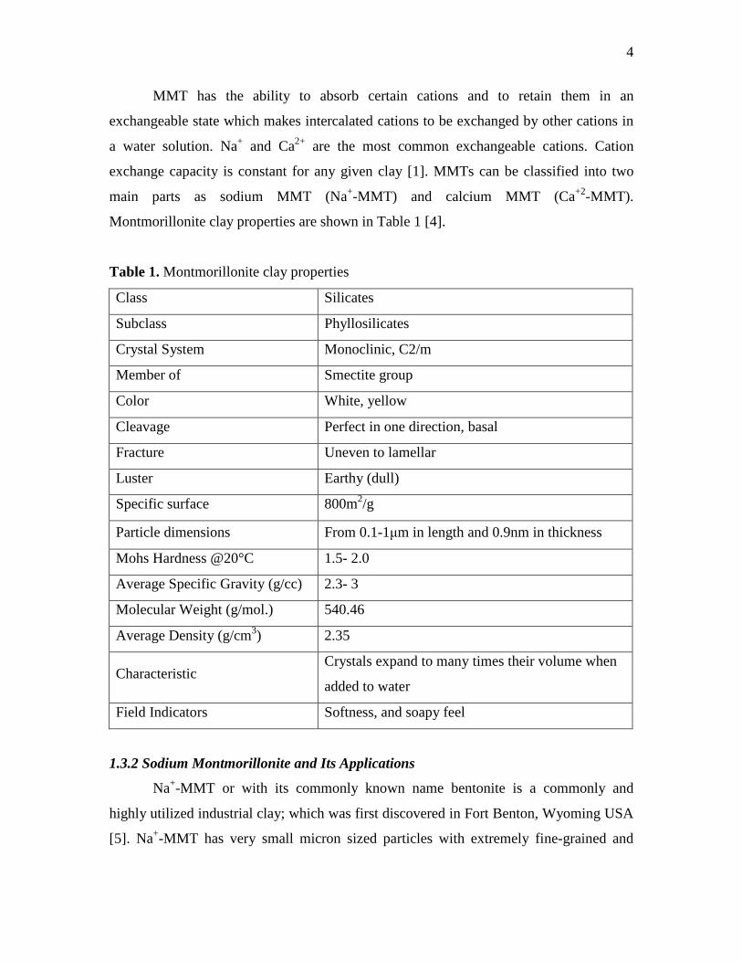
MMT has the ability to absorb certain cations and to retain them in an
exchangeable state which makes intercalated cations to be exchanged by other cations in
a water solution. Na+ and Ca2+ are the most common exchangeable cations. Cation
exchange capacity is constant for any given clay [1]. MMTs can be classified into two
main parts as sodium MMT (Na+-MMT) and calcium MMT (Ca+2-MMT).
Montmorillonite clay properties are shown in Table 1 [4].
Table 1. Montmorillonite clay properties
Class Silicates
Subclass Phyllosilicates
Crystal System Monoclinic, C2/m
Member of Smectite group
Color White, yellow
Cleavage Perfect in one direction, basal
Fracture Uneven to lamellar
Luster Earthy (dull)
Specific surface 800m2/g
Particle dimensions From 0.1-1µm in length and 0.9nm in thickness
Mohs Hardness @20°C 1.5- 2.0
Average Specific Gravity (g/cc) 2.3- 3
Molecular Weight (g/mol.) 540.46
Average Density (g/cm3) 2.35
Characteristic Crystals expand to many times their volume when
added to water
Field Indicators Softness, and soapy feel
1.3.2 Sodium Montmorillonite and Its Applications
Na+-MMT or with its commonly known name bentonite is a commonly and
highly utilized industrial clay; which was first discovered in Fort Benton, Wyoming USA
[5]. Na+-MMT has very small micron sized particles with extremely fine-grained and
Page 17
5
thin-layered structure. Within these thin layers loosely bonded Na+ cations present.
Loosely bonded Na+ cations are bound to one another and they are easily exchangeable.
Na+-MMT is the most developed and commercialized clay. Na+-MMT is naturally
hydrophilic and it has pretty good water affinity. Due to this property, they are
incompatible with most polymers. Consequently it is difficult to get good mixing and
dispersion of Na+-MMT with polymer solutions. Additionally, the high electrostatic
forces cause clay platelets to hold together tight [6]. For these reasons the clay must be
treated so it can be incorporated into a polymer. In order to make clay surface more
compatible with a polymer, ion exchanging method is a common application. On the
other hand ion dipole interaction is an alternative method to ion exchanging method. As
mentioned above, since the cations on the clay surface are loosely bound, they can be
replaced by other cations. This process makes clay more hydrophobic and helps clay
platelets to separate. When clay platelets are separated, they can be easily intercalated
and then subsequently exfoliated into the polymer [6].
Na+-MMT clays have several application areas. To list of them:
Binder of fodder (animal feeds) in pellet form.
Binder of insulating material containing rock wool or asbestos fibers which are
used in furnaces and steam boilers.
Plasticizing agent in cement and grout.
Plasticizer in brick, sewer pipe, ceramic, and refractory mixes.
Thickener of fire retardant slurries dropped from aircraft.
Thickener and stabilizer of latex and of rubber adhesives.
Thickening, suspending, and adsorptive ingredient in medicines, pharmaceuticals,
and cosmetics.
Gelling agent in greases and lubricants.
1.4 Synthetic Methods for Polymer Layered Clay Nanocomposites
Intercalation of polymers into inorganic layered materials with retention of the layered
structure is an excellent way of constructing novel inorganic-polymer composite systems.
Fig. 3 shows a schematic view of intercalation reactions of polymers into the interlayer
spaces. Intercalation is either done directly or done by in situ polymerization of pre-
Page 18
6
intercalated monomers between the layers of host materials. Since direct intercalation is
limited, preintercalated monomers becomes more important. However, control of
molecular weight of the polymers become more difficult in situ polymerization method
[7].
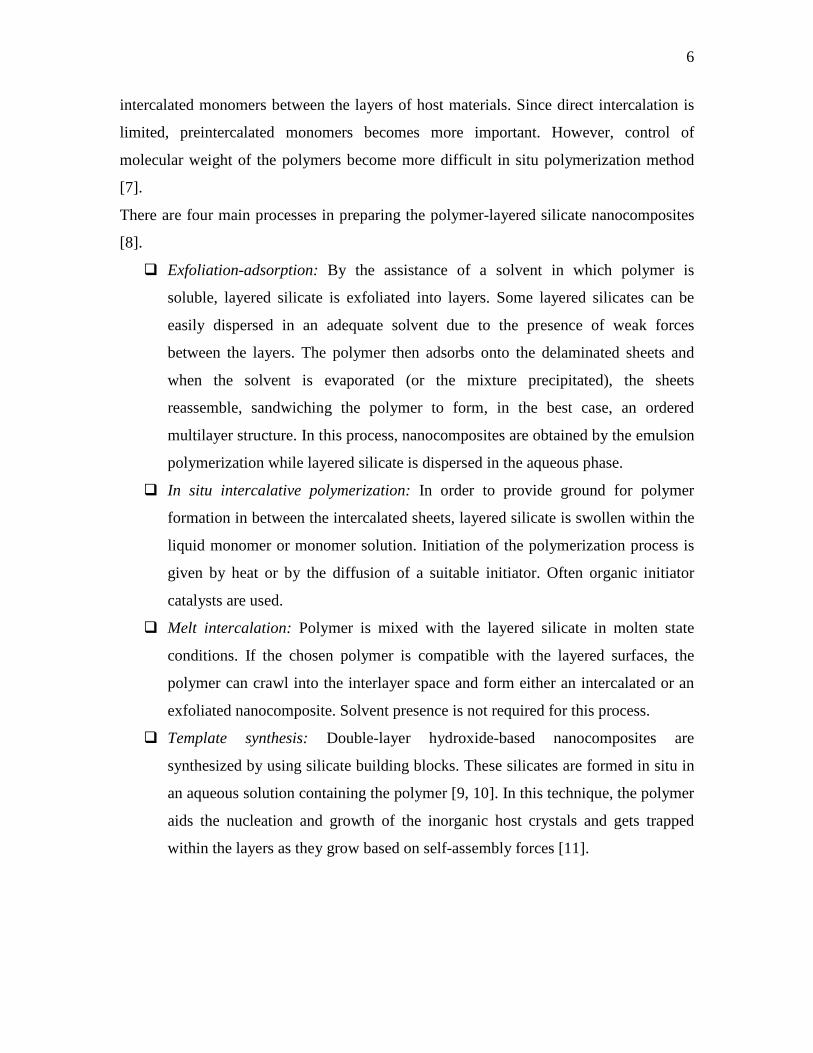
There are four main processes in preparing the polymer-layered silicate nanocomposites
[8].
Exfoliation-adsorption: By the assistance of a solvent in which polymer is
soluble, layered silicate is exfoliated into layers. Some layered silicates can be
easily dispersed in an adequate solvent due to the presence of weak forces
between the layers. The polymer then adsorbs onto the delaminated sheets and
when the solvent is evaporated (or the mixture precipitated), the sheets
reassemble, sandwiching the polymer to form, in the best case, an ordered
multilayer structure. In this process, nanocomposites are obtained by the emulsion
polymerization while layered silicate is dispersed in the aqueous phase.
In situ intercalative polymerization: In order to provide ground for polymer
formation in between the intercalated sheets, layered silicate is swollen within the
liquid monomer or monomer solution. Initiation of the polymerization process is
given by heat or by the diffusion of a suitable initiator. Often organic initiator
catalysts are used.
Melt intercalation: Polymer is mixed with the layered silicate in molten state
conditions. If the chosen polymer is compatible with the layered surfaces, the
polymer can crawl into the interlayer space and form either an intercalated or an
exfoliated nanocomposite. Solvent presence is not required for this process.
Template synthesis: Double-layer hydroxide-based nanocomposites are
synthesized by using silicate building blocks. These silicates are formed in situ in
an aqueous solution containing the polymer [9, 10]. In this technique, the polymer
aids the nucleation and growth of the inorganic host crystals and gets trapped
within the layers as they grow based on self-assembly forces [11].
Page 19
7
.
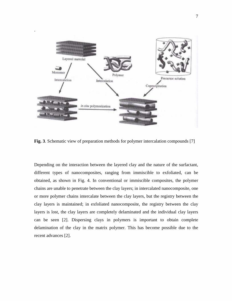
Fig. 3. Schematic view of preparation methods for polymer intercalation compounds [7]
Depending on the interaction between the layered clay and the nature of the surfactant,
different types of nanocomposites, ranging from immiscible to exfoliated, can be
obtained, as shown in Fig. 4. In conventional or immiscible composites, the polymer
chains are unable to penetrate between the clay layers; in intercalated nanocomposite, one
or more polymer chains intercalate between the clay layers, but the registry between the
clay layers is maintained; in exfoliated nanocomposite, the registry between the clay
layers is lost, the clay layers are completely delaminated and the individual clay layers
can be seen [2]. Dispersing clays in polymers is important to obtain complete
delamination of the clay in the matrix polymer. This has become possible due to the
recent advances [2].
Page 20
8
Fig. 4. Scheme of different types of composite arising from the interaction of polymers
and layered nanocomposites[12]
Page 21
9
CHAPTER II
THEORY
2.1 Introduction to Molecular Simulation
After the end of 2nd World War, the use of computers and associated
computational methods in solving problems in science and engineering have grown
dramatically and leading to emerging fields such as computational physics,
computational chemistry, computational fluid dynamics, computational solid mechanics,
etc. as the computational methods become feasible [1, 2, 13-15]. As the high performance
computers with increasing efficiency become available, scientists and engineers are
handling modeling and simulations approaches to problems using levels of methods
ranging from quantum level calculations to chemical plant design. In this study, we shall
focus our attention only on the atomic or molecular scale simulations, which covers the
time scale up to a few tens of nano-seconds and the length scale up to a few tens of
nanometers.
Molecular simulations play a crucial role especially in nanoscale research due to
compatible nature of length and time scales involved. In general, one may use molecular
simulation approaches to compare the calculated properties of systems with the
experimental results. But even more important, molecular simulations can be employed
to the systems that have not been studied via experiments [13, 15] in order to aid or guide
the development of new material systems and structures. This, of course, requires
enhancing the predictive power of molecular simulations. In classical molecular
simulations this requires improvement of the functional form and parameterization of the
intermolecular and intramolecular interactions underlying the physics and chemistry of
the materials systems. The functional forms and associated parameters, i.e. the force-
fields, may be improved by validating the simulation results against the experiments.
With reliable interaction force fields, molecular simulations can be used to guide the
physical experiments. Furthermore, molecular simulations served as a test method for
new theories of condensed phases of matter by theoreticians. That is to say, in this case
simulations may be used to screen the theories and play the role of testing by
experiments. Therefore, we may refer to a molecular simulation processes as computer
Page 22
10
‘virtual’ experiments [13]. Molecular dynamics (MD) simulation and Monte Carlo (MC)
simulation are the two basic techniques in the molecular simulation world.
Through molecular simulations with reliable interaction force fields, the
macroscopic thermodynamic properties such as pressure, internal energy, thermal
expansion, compressibility, tensile and shear modulus, specific heats can be evaluated by
using the microscopic level information generated through simulations [15]. For instance,
the equilibrium macroscopic properties are calculated by taking the averages or time
averages in molecular dynamics,, and ensemble averages in Monte Carlo simulations. On
the other hand, transport macroscopic properties - often referred as dynamic properties-,
can be measured from molecular dynamics simulation using appropriate time correlation
functions of the relevant microscopic variables over the generated time series -trajectory.
2.2 Molecular Dynamics
Molecular dynamics first introduced by Alder and Wainwright [16], in order to
study the condensed phase of fluids beyond the gas state densities. Early simulations
utilized hard core represantation for interactions, In 1964 Rahman [17] carried out first
simulation including long range interactions (soft sphere) by employing Lennard-Jones
potential to represent the interactions in liquid argon as opposed to hard sphere . Since
then the molecular dynamics simulations with continuous potentials became a very
widely used research tool for researcher to calculate the bulk properties of materials and
to develop fundamental physical understanding of systems including complex systems
such as biological and synthetic polymers.
The theoretical basis in using molecular modeling in relating atomistic trajectories
in space to macroscopic physico-chemical properties is statistical thermodynamics.
Hence, through determining the structure and dynamics of a system at the atomistic level
one can predict the bulk property of a system at the macroscopic level. One approach to
establish this connection is through molecular dynamics (MD). MD generates
information at the atomistic level by producing a time series of positions and momenta of
these particles through which one can determine the physical properties. The time series
for position and momenta –trajectory – is obtain via solving the Newtonian equations of
motion for an N-body system.
Page 23
11
The equations of motion is simply the statement of Newton’s second law for each
particle in N-body systems,
Force = mass * acceleration or Fi = mi * ai , (1)
Here the force on a given particle is a function of the coordinates of the other particles in
the N-body system. Hence the equations of motion are iteratively solved in time as the
positions and velocities of particles change. The force on any atom is calculated from the
derivative of energy at each configuration –for a system under no external force:
ii
Fdr
dE =− (2)
One may evaluate the energies and forces using a classical force fields or a seleted level
of quantum theory. In practice, the atoms are assigned initial velocities that conform to
the total kinetic energy of the system, which in turn, is dictated by the desired simulation
temperature. From the knowledge of the force on each atom, it is possible to determine
the acceleration of each atom in the system. Integration of the equations of motion then
yields a trajectory that describes the positions, velocities and accelerations of the particles
as they vary with time. From this trajectory, the average values of properties can be
determined. The method is deterministic; once the positions and velocities of each atom
are known, the state of the system can be predicted at any time in the future or the past.
Molecular dynamics simulations can be time consuming and computationally expensive.
However, computers are getting faster and cheaper. Simulations of solvated proteins are
calculated up to the nanosecond time scale; however, simulations into the millisecond
regime have been reported.
Identification and evaluation of different type of interactions between different
types of particles is expressed through what we call the force fields. There are many types
of force field. We will describe some of the widely used force fields below. In our
calculations we have used a force field which accurately represents the interactions
within clay and interactions with organic molecules and polymers and within organic
polymers.
Page 24
12
2.2.1 Force Fields
The functional form of the potential energy expression and the entire set of
parameters needed to fit the potential energy surface constitute the force field. The energy
expression is the specific equation that is set up for a particular model (types of atoms,
particular connectivity, choices for attributes, etc) and including (or not) any optional
terms.
It is important to understand that the force field both the functional form and the
parameters themselves represents the single largest approximation in molecular
modeling. The quality of the force field, its applicability to the model at hand, and its
ability to predict the particular properties measured in the simulation directly determine
the validity of the results.
The force field contains the necessary building blocks for the calculations of
energy and force:
A list of atom types.
A list of atomic charges (if not included in the atom-type information).
Atom-typing rules.
Functional forms for the components of the energy expression.
Parameters for the function terms.
For some force fields, this may include some rules for generating parameters that
have not been explicitly defined.
For some force fields, this may include a specified way of assigning the functional
forms and associated parameters.
The force fields commonly used for describing molecules, polymers, biopolymers
usually employ a combination of internal coordinates and terms (bond distances, bond
angles, torsions, etc.), to describe part of the potential energy surface due to interactions
between bonded atoms, and nonbond terms to describe the van der Waals and
electrostatic interactions between atoms. The functional forms range from simple
quadratic forms to Morse functions, Fourier expansions, Lennard–Jones potentials, etc.
The goal of a force field is to describe entire classes of molecules with reasonable
accuracy. In a sense, the force field interpolates and extrapolates from the empirical data
of the small set of models used to parameterize the force field to a larger set of related
Page 25
13
models. Some force fields aim for high accuracy for a limited set of element types, thus
enabling good prediction of many molecular properties. Other force fields aim for the
broadest possible coverage of the periodic table, with necessarily lower accuracy.
2.2.1.1 The Energy Expression
The actual coordinates of a model combined with the force field data create the
energy expression (or target function) for the model. This energy expression is the
equation that describes the potential energy surface of a particular model as a function of
its atomic coordinates. The potential energy of a system can be expressed as a sum of
valence (or bond), and nonbonded interactions.
The energy of valence interactions is generally accounted for by diagonal terms,
namely, bond stretching (Ebond), valence angle bending (Eangle), dihedral angle torsion
(Etorsion), and inversion (Einversion) terms, which are part of nearly all force fields for
covalent systems.
Eval = Ebond + Eangle + Etorsion + Einv (3)
The energy of interactions between nonbonded atoms is accounted for by van der
Waals (EvdW), electrostatic (ECoulomb), and (in some older force fields) hydrogen bond
(Ehbond) terms:
Enonbond = EvdW + ECoulomb + Ehbond(4)
2.2.1.2 Advantages of Having Several Force Fields
A broader range of systems can be treated: Some classical force fields were
originally created for modeling proteins and peptides, others for DNA and RNA. Some
have been extended to handle more general systems having similar functional groups.
The rule-based force fields have extended the range of force field simulations to a
broader range of elements. The second-generation force fields currently include
parameters for all functional groups appropriate for protein simulations.
Identical calculations with two or more independent force fields can be compared
to assess the dependence of the results on the force field: For example, amino acid
parameters are defined in the AMBER, CHARMm, CVFF, CFF, and MMFF94 force
Page 26
14
fields, so peptide and protein calculations with these force fields can be compared to
assess the effect of the force fields.
The different functional forms used in the various energy expressions increase the
flexibility of molecular mechanics or molecular dynamics program: You can balance the
requirements of high accuracy vs. available computational resources. (Highly accurate
force fields are generally more complex and therefore require more resources.) Different
energy terms can be compared. For example, approximations such as a distance-
dependent dielectric constant or scaling of 1–4 nonbond interactions can be assessed.
Harmonic bond terms are accurate only at bond lengths close to the reference bond
length, but the Morse term can be used to model bond breaking.
The development of new force fields and elsewhere continues to provide more
accurate and more broadly applicable force fields. As experience is gained in
parameterizing the force fields and as new experimental data become available, the range
of both properties and systems fit by these newer force fields will increase.
2.2.1.3 Types of Force Field
Many different force fields which are suitable for systems dealt in this thesis
exists, such as CHARMM, AMBER, Dreiding, CFF, PCFF, Universal, CVFF. These are
some of the most frequently used force fields. Based upon need and target system it’s a
referred practice to modify an existing force field in order to get the best values out of it.
Sometimes on may also go to an extent to develop a separate force field to suit the needs
of the specific research.
Force fields are classified in different classes. There are second generation force
fields developed by high parameterization (examples CFF, PCFF COMPASS etc), rule
based force fields like Universal and Dreiding where parameters are decided by some
rules (example hybridization), classical or first generation force field like AMBER,
CHARMM and CVFF which is also based on parameterization but mostly from
experimental values as oppose to that of second generation which is based on quantum
input and special purpose force field.
CVFF force field is also based on parameterization but mostly from experimental
values as oppose to that of second generation which is based on quantum input and
Page 27
15
special purpose force field. CVFF includes harmonic bond stretching and bond angle
bending terms, a shifted 12-6 Lennard Jones potential for nonbonded interactions, and a
Coulombic term for interactions between atom-centered partial atomic charges [18].
[ ] ∑∑ ∑∑∑ +
−
+++−+−=
jiij
ji
ji ijijbbpot
r
qq
r
B
r
AnskkbbkE
,,
612
20
20 )cos(1)()(
εεφθθ
φφ
θθ (5)
where kb, kθ, kΦ are force constants, n is multiplicity and Φ is the phase angle for the
torsional angle parameters. The A, B, and q parameters are the nonbonded potentials.
AMBER force field is widely used for simulation of proteins and nucleic acids [19].
First term of Eq 6 (summing over bonds) represents the energy between covalently
bonded atoms. This harmonic (ideal spring) force is a good approximation near the
equilibrium bond length, but becomes increasingly poor as atoms separate. Second term
(summing over angles): represents the energy due to the geometry of electron orbitals
involved in covalent bonding. Third term (summing over torsions): represents the energy
for twisting a bond due to bond order (e.g. double bonds) and neighboring bonds or lone
pairs of electrons. Note that a single bond may have more than one of these terms, such
that the total torsional energy is expressed as a Fourier series. Fourth term (double
summation over i and j): represents the non-bonded energy between all atom pairs, which
can be decomposed into van der Waals (first term of summation) and electrostatic
(second term of summation) energies. The form of the electrostatic energy used here
assumes that the charges due to the protons and electrons in an atom can be represented
by a single point charge. (Or in the case of parameter sets that employ lone pairs, a small
number of point charges.)
[ ] ∑∑ ∑∑∑ +
−
+−++−+−=
jiij
ji
ji ijij
n
bbpot
r
qq
r
B
r
Ank
vkllkE
,,
612
20
20 )cos(1
2)(
2
1)(
2
1
εγφθθ
φφ
θθ (6)
In Eq 6, kb, kθ, kΦ are force constants, n is multiplicity and Φ is the phase angle for the
torsional angle parameters. The A, B, and q parameters characterize the nonbonded
potentials.
CHARMM (a general and flexible software application for modeling program for
studying the structure and behavior of molecular systems ranging from an individual
Page 28
16
organic molecule to large proteins in its solvent environment) uses similar energy
functions as the others with parameterized extensively using empirical data for energy
minimization, molecular dynamics simulation, or vibrational analysis. In these
specialized force fields, there are often understated differences in force constants and
geometric parameters for similar atoms in slightly different environments, and it is often
not clear how to generalize for new atoms or new bond types.
EBond= kl ( l-lo )2(7)
Eangle = kθ ( θ-θo )2(8)
)]cos(1[ Φ−= Φ JKrotate nkE (9)
∑
−
=
612
4ij
ij
ij
ijvdW RR
Eσσ
ε (10)
There are cases for reliable molecular modeling the first steps to be pursued is the
development of a force field that contains parameters characterize the interactions more
accurately than the existing force field models. In the present work we employ this kind
of a force fields to represent the interactions between clay particles and polymers: In
particular we employ the Morse-Stretch Charge Equilibration Force Field (MSQ) for the
interactions within inorganic components [20] and supplement it with the Dreiding Force
Field type for the interactions within the organic component [21]. The mixed non-bond
organic-inorganic interactions (electrostatic and van der Waals) are separately calculated
and added. One of the important features of these force fields is that the atomic charges
are allowed to readjust instantaneously to the atomic configurations. These charges are
calculated using the charge equilibration (QEQ) method [22].
2.2.1.3.1 Dreiding Force Field [21]
The source of the force field used for the organic interactions is a widely used
force field known as Dreiding [21]. This force field was chosen because property
predicted for polymer systems using this force field has given good agreement with the
experimental values in the past [23, 24]. Just like any other force fields attempting to
describe organics, Dreiding also employs different functions for describing the
interaction energy. The energy of a system can be written as the sum of two components
Page 29
17
and each component has multiple contributions deriving from the topology of organics
molecules involved. Below, we give a summary of these terms:
E = EVAL + ENB where(11)
EVAL = EB + EA + ET + EI (12)
ENB = EVDW + ECoul + EHB (13)
EB = Energy due to Bond stretching (two body)
EA = Energy due to angle bending (three body)
ET = Energy due to torsion (four body)
EI = Energy due to out of plane configuration (four body)
EVDW = Energy due to van der Waals interaction
ECoul = Energy due to columbic interaction
EHB = Energy due to hydrogen bonding
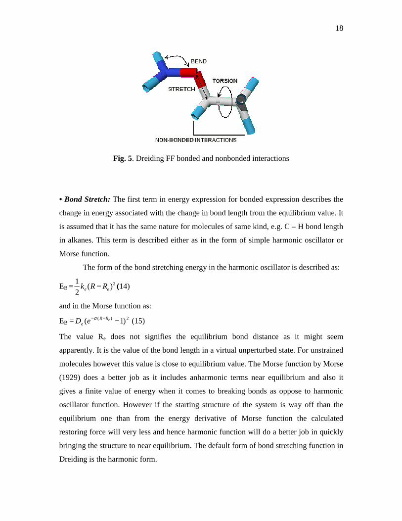
The first four terms are due to bonded interaction the last two terms are due to
nonbonded interactions (Fig. 5). All these terms will be discussed in little more detail in
the following sections. It is this calculation of electrostatic interaction terms takes most of
the simulation time. The simple reason being as this interaction can happen between any
two atoms, ideally this calculation should be carried out for each atom and hence it takes
time in the order of N2 where N is the number of atoms of the system. These interactions
are also called long range interactions as they die out inversely with the value of ‘r’ and
hence contributes some value till a large value of ‘r’. Algorithms have been developed for
handling the problem in such a way so that simulation time can be decreased without
sacrificing the accuracy of the results as such. While length of simulation is one
important aspect the other one is the time step used for the simulation. Ideally the time
step in a simulation should be such that it can capture the fastest motion in the system
which is typically the vibration mode. Typically time step in the order of 0.1 fs to 10 fs
are used depending upon the system involved in the simulation. Sometimes in simulation
the fastest parts are treated as constant and this enables one to take a longer time step and
hence accelerating the whole process.
Page 30
18
Fig. 5. Dreiding FF bonded and nonbonded interactions
• Bond Stretch: The first term in energy expression for bonded expression describes the
change in energy associated with the change in bond length from the equilibrium value. It
is assumed that it has the same nature for molecules of same kind, e.g. C – H bond length
in alkanes. This term is described either as in the form of simple harmonic oscillator or
Morse function.
The form of the bond stretching energy in the harmonic oscillator is described as:
EB =2)(
21
ee RRk − (14)
and in the Morse function as:
EB = 2)( )1( −−− eRRe eD α (15)
The value Re does not signifies the equilibrium bond distance as it might seem
apparently. It is the value of the bond length in a virtual unperturbed state. For unstrained
molecules however this value is close to equilibrium value. The Morse function by Morse
(1929) does a better job as it includes anharmonic terms near equilibrium and also it
gives a finite value of energy when it comes to breaking bonds as oppose to harmonic
oscillator function. However if the starting structure of the system is way off than the
equilibrium one than from the energy derivative of Morse function the calculated
restoring force will very less and hence harmonic function will do a better job in quickly
bringing the structure to near equilibrium. The default form of bond stretching function in
Dreiding is the harmonic form.
Page 31
19
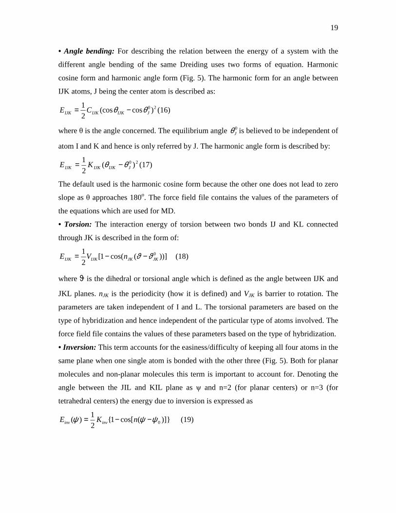
• Angle bending: For describing the relation between the energy of a system with the
different angle bending of the same Dreiding uses two forms of equation. Harmonic
cosine form and harmonic angle form (Fig. 5). The harmonic form for an angle between
IJK atoms, J being the center atom is described as:
20)cos(cos21
JIJKIJKIJK CE θθ −= (16)
where θ is the angle concerned. The equilibrium angle 0Jθ is believed to be independent of
atom I and K and hence is only referred by J. The harmonic angle form is described by:
20 )(2
1JIJKIJKIJK KE θθ −= (17)
The default used is the harmonic cosine form because the other one does not lead to zero
slope as θ approaches 180o. The force field file contains the values of the parameters of
the equations which are used for MD.
• Torsion: The interaction energy of torsion between two bonds IJ and KL connected
through JK is described in the form of:
))](cos(1[2
1 0JKJKIJKIJK nVE ϑϑ −−= (18)
where ϑ is the dihedral or torsional angle which is defined as the angle between IJK and
JKL planes. nJK is the periodicity (how it is defined) and VJK is barrier to rotation. The
parameters are taken independent of I and L. The torsional parameters are based on the
type of hybridization and hence independent of the particular type of atoms involved. The
force field file contains the values of these parameters based on the type of hybridization.
• Inversion: This term accounts for the easiness/difficulty of keeping all four atoms in the
same plane when one single atom is bonded with the other three (Fig. 5). Both for planar
molecules and non-planar molecules this term is important to account for. Denoting the
angle between the JIL and KIL plane as ψ and n=2 (for planar centers) or n=3 (for
tetrahedral centers) the energy due to inversion is expressed as
)](cos[121
)( 0ψψψ −−= nKE invinv (19)
Page 32
20
• Nonbonded Interactions: There are two expressions by which nonbonded van der
waals interactions are described. Lennard – Jones (LJ) 12 -6 forms and the exponential 6
form. The LJ form is described as:
612 −− −= BRARELJvdw (20)
and the exponential 6 form described as:
66 −− −= BRAeE CRXvdw (21)
As can be seen the difference between the two forms is nothing but the way of describing
the repulsive part. For very low distance between two atoms the LJ potential gives a very
big repulsive force and hence throws the atoms away. Though the LJ potential however
requires only two parameters for the evaluation of the potential and faster to compute
(find out the reason) the exponential 6 form gives a better agreement for short range
interactions. The default form used in Dreiding is however LJ. The parameter values are
calculated differently if the interaction concerned is between two different types of
atoms. The way it is calculated can be based on arithmetic or geometric combination of
the parameters of the pure system.
• Electrostatic interactions: The interaction energy due to electrostatic interactions is
calculated by:
ij
jiq r
qqkE = (22)
where qi and qj are the charges on the atoms and rij is the distance between them. k is a
constant which takes care of the dielectric constant and unit consideration. Interactions
are not calculated for atoms bonded to each other (1, 2 interaction) and those involved in
angle terms (1, 2, 3 interactions) as these are taken care by bond and angle stretching
interactions.
• Hydrogen Bonding: The center of charges and van der Waals interaction must be in the
center of the atom in order to take the position of the point charge on an atom and center
of the atom to be the same. Satisfying this constraint it is difficult to parameterize a force
field which correctly predicts the structure and the bond energy of H2O dimer, predicts
the sublimation energy and the structure of ice and using van der Waals parameter
correctly for non hydrogen bonded system. Dreiding uses a separate term to account for
hydrogen bonding to describe interaction involving hydrogen atom with that of very
Page 33
21
electronegative atoms (N, O, F) associated with hydrogen bond. In that case in addition to
van der Waals forces and electrostatic interactions, a hydrogen bonding potential of the
following form is included.
)(cos])(6)(5[ 41012DHA
DA
hb
DA
hbhbhb R
R
R
RDE θ−= (23)
where θDHA is the bond angle between hydrogen donor (D), hydrogen (H) and hydrogen
acceptor (A). RDA is the distance between donor and acceptor atoms and the values of Dhb
and Rhb depends on the convention for assigning charges.
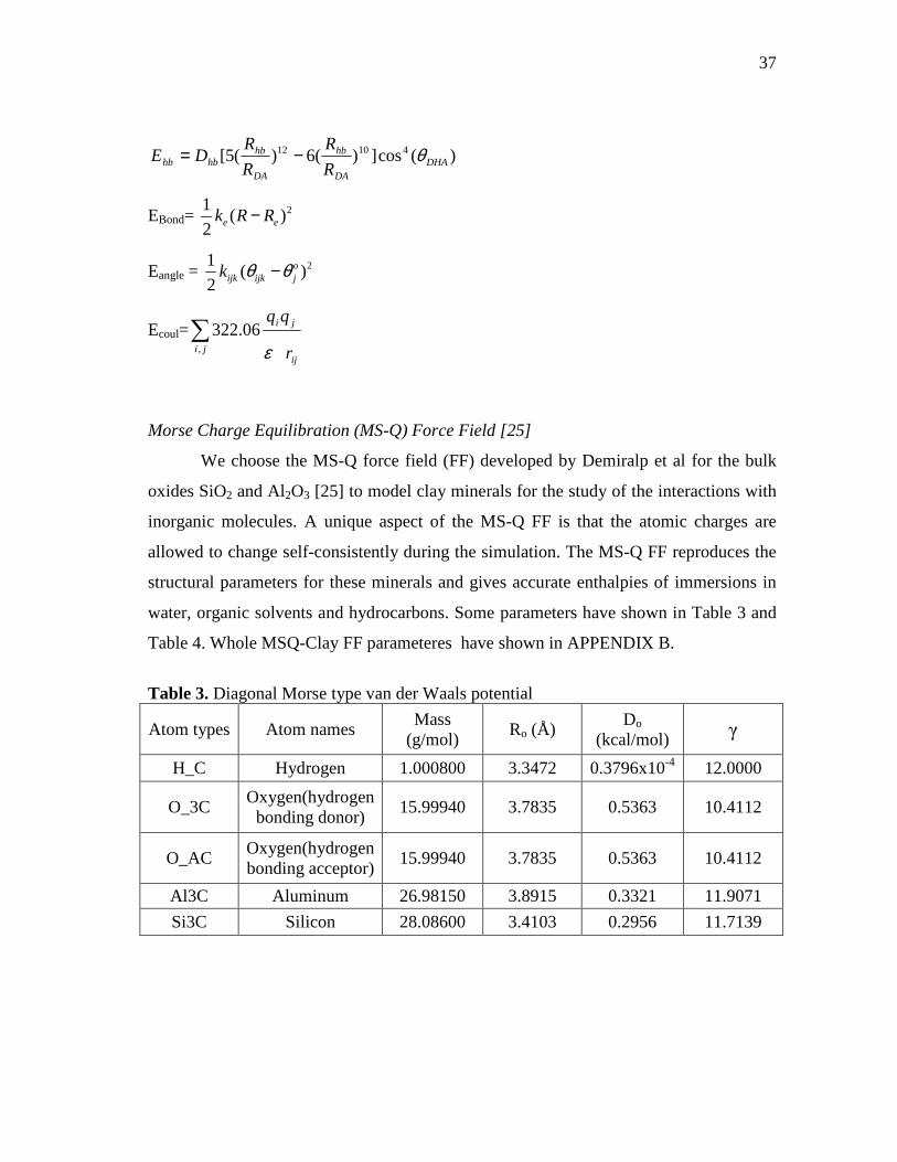
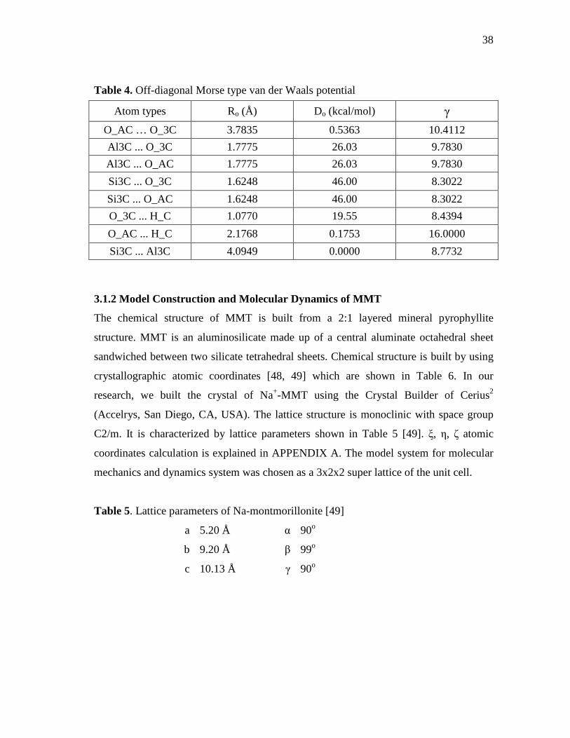
2.2.1.3.2 Morse Charge Equilibration (MS-Q) Force Field [25]
A Morse-charge equilibration force field (MS-Q FF) originally built up for bulk oxides
Al 2O3 and SiO2. MS-Q FF has been used for modeling clay minerals and their
interactions with representative organic molecules.
The concept behind MS-Q is that for ionic or polar materials, electrostatics is the
dominant force determining the structure and properties of the material. However, the
charges responsible for the electrostatic effects depend upon the atomic configuration of
the neighboring atoms [26]. The MS-Q FF allows the atomic charges to readjust as a
function of the instantaneous geometry using the charge equilibration (QEq) procedure
[22] of Rappé and Goddard. In addition, to electrostatic interactions, MS-Q uses a two
body Morse function to describe nonelectrostatic terms [27].
−−−
−−= 1
2exp21exp)(
000 R
R
R
RDRE ijij
ijMorseij
γγ (24)
Thus potential energy that is the interaction between atom i and j is given by
[ ]
−−=
+−=
12
expwhere
)25(2)(
0
20
R
R
R
qqDRU
ijijij
ij
jiijijijijij
γχ
χχ
where D0ij is the bond strength in kcal/mol, R0ij is the bond distance in Ǻ, ijγ is a scale
factor, and qi is the partial charge if i th atom [28].
Page 34
22
Originally Morse-stretch potential charge equilibrium force field (MS-Q FF) has
been developed to predict the phase changes in ionic insulators such as minerals and
ceramics. The proposed MS-Q FF for silica system describes both four-fold and six-fold
coordinated systems, silica glass and pressure-induced phase changes. It has been applied
to various zeolites, silicates and alumina-silicates [28] and high pressure behavior of
geophysical materials [29].
2.2.2 Ensembles
In mathematical physics, especially as introduced into statistical mechanics and
thermodynamics by J. Willard Gibbs in 1878, an ensemble (also statistical ensemble or
thermodynamic ensemble) is an idealization consisting of a large number of mental
copies (possibly infinitely many) of a system, considered all at once, each of which
represents a possible state that the real system might be in.
The ensemble formalizes the notion that a physicist can imagine repeating an
experiment again and again under the same macroscopic conditions, but, unable to
control the microscopic details, may expect to observe a range of different outcomes.
When an ensemble has an infinite number of members, it can be seen as defining
a probability measure on the state space (phase space) of the system. Even though the
dynamics of the real single system (for example, a complete gas of molecules, or a
complete stock market) may be incalculably complex, or stochastic, or even
discontinuous, the average (statistical) properties of the ensemble of possibilities as a
whole may remain well defined, smoothly evolving, or for systems at macroscopic
equilibrium even stationary. The notional size of the mental ensembles in
thermodynamics, statistical mechanics and quantum statistical mechanics can be very
large indeed, to include every possible microscopic state the system could be in,
consistent with its observed macroscopic properties. But for important physical cases it
can be possible, by clever mathematical manipulations, to calculate averages directly
over the whole of the thermodynamic ensemble, to obtain explicit formulas for many of
the thermodynamic quantities of interest, often in terms of the partition function Z, which
encodes the underlying physical structure of the system [30].
Page 35
23
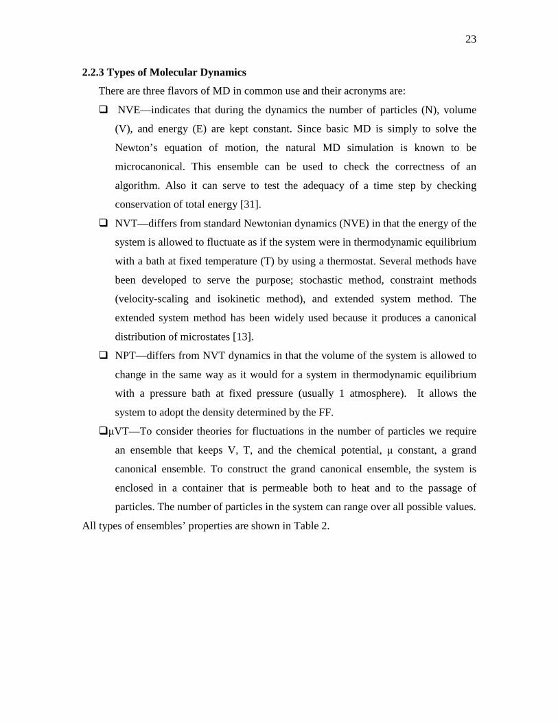
2.2.3 Types of Molecular Dynamics
There are three flavors of MD in common use and their acronyms are:
NVE—indicates that during the dynamics the number of particles (N), volume
(V), and energy (E) are kept constant. Since basic MD is simply to solve the
Newton’s equation of motion, the natural MD simulation is known to be
microcanonical. This ensemble can be used to check the correctness of an
algorithm. Also it can serve to test the adequacy of a time step by checking
conservation of total energy [31].
NVT—differs from standard Newtonian dynamics (NVE) in that the energy of the
system is allowed to fluctuate as if the system were in thermodynamic equilibrium
with a bath at fixed temperature (T) by using a thermostat. Several methods have
been developed to serve the purpose; stochastic method, constraint methods
(velocity-scaling and isokinetic method), and extended system method. The
extended system method has been widely used because it produces a canonical
distribution of microstates [13].
NPT—differs from NVT dynamics in that the volume of the system is allowed to
change in the same way as it would for a system in thermodynamic equilibrium
with a pressure bath at fixed pressure (usually 1 atmosphere). It allows the
system to adopt the density determined by the FF.
µVT—To consider theories for fluctuations in the number of particles we require
an ensemble that keeps V, T, and the chemical potential, µ constant, a grand
canonical ensemble. To construct the grand canonical ensemble, the system is
enclosed in a container that is permeable both to heat and to the passage of
particles. The number of particles in the system can range over all possible values.
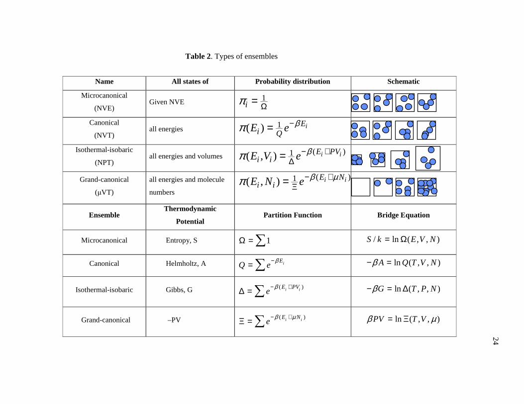
All types of ensembles’ properties are shown in Table 2.
Page 36
24
Name All states of Probability distribution Schematic
Microcanonical
(NVE) Given NVE 1
iπ Ω=
Canonical
(NVT) all energies 1( ) iE
i QE e βπ −=
Isothermal-isobaric
(NPT) all energies and volumes
( )1( , ) i iE PVi iE V e βπ − +
∆=
Grand-canonical
(µVT)
all energies and molecule
numbers
( )1( , ) i iE Ni iE N e β µπ − +
Ξ=
Ensemble Thermodynamic
Potential Partition Function Bridge Equation
Microcanonical Entropy, S 1Ω = ∑ / ln ( , , )S k E V N= Ω
Canonical Helmholtz, A iEQ e
β−= ∑ ln ( , , )A Q T V Nβ− =
Isothermal-isobaric Gibbs, G ( )i iE PVe
β− +∆ = ∑ ln ( , , )G T P Nβ− = ∆
Grand-canonical –PV ( )i iE Ne
β µ− +Ξ = ∑ ln ( , , )PV T Vβ µ= Ξ
Table 2. Types of ensembles
Page 37
25
2.3 Ab-Initio Calculations
Methods using the Hartree-Fock or DFT to calculate the electronic structure and
associated properties are called ab-initio or first principles calculations, i.e. without the
need for empirical fitting parameters. Ab-initio calculations are computationally costly.
Though theories associated with ab-initio calculations were developed several decades
ago, only in the last two decades ab-initio calculations have developed into one of the
most important methods in atomistic modeling mostly due to more and more powerful
computational resources become available.
The ab-initio methods are usually used to calculate the band structure, associated
properties with the band structure, electronic and magnetic properties of systems, the
phonon dispersion and thermal properties. Combined with MD, MC, transition state
theory (TST), such as the nudged elastic band (NEB) method, ab-initio methods are also
capable of simulating dynamic and kinetic problems.
2.3.1 Density Functional Theory
Density functional theory (DFT) is a formalism which allows the description of a
system in terms of its electron density,
→rρ . Based on the Hohenberg-Kohn theorem,
the total electron energy can be written as a unique functional of the electron density,
E[
→rρ ] [32]. The variational principle can be used to minimize the energy functional
with respect to the density [33, 34],
0=
∂
∂
→
→
r
rE
ρ
ρ (26)
The total energy of an N-electron system contains the kinetic energy
K[
→rρ ],electron-nuclei interactions Eel-nucl[
→rρ ],electron-electron interactions Eel-
el[
→rρ ],and the exchange-correlation energy EXC[
→rρ ],
Page 38
26
E[
→rρ ] = K[
→rρ ] + Eel-nucl[
→rρ ] + Eel-el[
→rρ ] + EXC[
→rρ ] (27)
where, Eel-nucl[
→rρ ] = ∫ rdrVext
3)(ρ and Eel-el[
→rρ ] =
′
→
→∫ ∫
′→
−→
′
→
r3dr
3d
rr
rρ(r)ρ
2
1
and extV is the external potential.
Since the functional dependence of the kinetic energy on the charge density is
unknown, practical calculations need to use both the charge density and the wave
functions, for which the kinetic energy can be easily calculated. Since the true many-
electron wave function is computationally too demanding, the wave function is
approximated by a linear combination of products of one-electron wave functions within
an effective potential, consisting of the nuclei and the other electrons. Since such a one-
electron approximation ignores the crucial electron-electron interactions, exchange and
correlation, an approximation is needed to correct this error. The two most common
approximations used today are called the local density approximation (LDA) and the
generalized gradient approximation (GGA) [32].
LDA assumes that at each point →r , the exchange-correlation energy equals that of
a system with constant ρ =
→rρ . GGA, however, has an explicit dependence of the
exchange-correlation functional on the gradient of the electron density. Both LDA and
GGA are generally successful in a large variety of applications. However, LDA has a
general tendency to overbinding. GGA has been shown to be quite successful in
correcting some of the deficiencies of LDA. However, there are cases where the GGA
may over-correct the deficiencies and lead to underbinding.
No matter if it is LDA or GGA, the total exchange-correlation energy of a system
is the sum of the exchange-correlation energies per particle, єxc[
→rρ ] (in the integral
form):
Page 39
27
rrrr d→→→→
∈=
∫
3XCXCE ρρρ (28)
Combining Eq. 26 to Eq. 28, variation of the total energy functional is
→∂
→∂
+
→+′
→∫
′→
−→
→
+
→∂
→∂
=
→∂
→∂
rρ
rρxcE
rextVr3d
rr
rρ
rρ
rρK
rρ
rρE (29)
where
→∂
→∂
+
→+′
→∫
′→
−→
→
=
→
rρ
rρxcE
rextVr3d
rr
rρ
reffV is defined as the effective
potential for the one-electron approximation. As mentioned earlier, the exact K[
→rρ ] in
Eq. 29 is unknown. However, it can be calculated from the wave functions. To minimize
the energy in Eq. 29, we guess initial wave functions, calculate
→rρ from them and plug
them into the Schrödinger equation to obtain a new wave function set, electron density
and
→
reffV , and then solve the Schrödinger equation again with the newly generated
→
reffV and wave functions until it is converged. These are self-consistent cycles known
as the Kohn-Sham equations (Fig. 6).
Page 40
28
Fig. 6. Schematic illustration of the self-consist cycles in ab initio calculations
In the Kohn-Sham equations, the wave functions are expanded into a basis for
computational efficiency. The most common wave function basis for periodic systems
consists of plane waves, a 3-D Fourier series
∑→
++
→=
G
rGkiGkk ear )(ψ (30)
where ak+G is a constant, k is a wave vector in the Brillouin zone, G represents a lattice
vector in reciprocal space.
However, calculations involving all electrons are still time-consuming. Since the
valence electrons (electrons located in incompletely filled shells, e.g. 3s2 and 3p2
electrons for Si) dominate bonding, calculations are usually restricted to the valence
electrons. All the effects of the core electrons (electrons in completely filled shell, such as
1s2, 2s2, and 2p6 electrons for Si) and nuclei are incorporated into an effective potential, a
so-called pseudopotential [35]. The computers today are capable of conducting ab-initio
calculations using pseudopentials and a plane wave basis set on systems with 3000 atoms.
The ab-initio calculations within this dissertation are primarily performed by using the
Vienna Ab-initio Simulation Package (VASP) [36, 37]. VASP is a complex package for
performing ab-initio quantum-mechanical calculations and molecular dynamic (MD)
simulations using pseudopotentials and a plane wave basis set. Due to its completeness,
Page 41
29
efficiency, and open-source distribution, it is probably the most widely used code of its
kind today. The detailed algorithms and performance of VASP are well documented on
its website cms.mpi.univie.ac.at/vasp/vasp/vasp.html. VASP calculations are known to
obtain accurate bonding energies, structural configurations, system energies, phonon
dispersions [38, 39], band structures (apart from the band gap, which is predicted smaller
than experiments due to neglecting the true exchange effects), and density of states
(DOS) of systems.
2.3.2 Advantages and Limitations of Ab-Initio Calculations
The ab-initio methods are based on solving the electronic Schrödinger equation.
Compared with empirical pair potentials and semi-empirical methods, it has the following
advantages:
a) No experimental bias;
b) Prediction of novel structures (no experimental data are required);
c) Calculating more accurate data and
d) Providing electronic states.
Ab-initio calculations are computationally expensive. Even today’s fastest
supercomputers can only conduct ab-initio calculation using pseudopotentials and a plane
wave basis set on systems with no more than a few thousand atoms. More practically, the
system is constrained to several hundred atoms. Obviously, it is thus impossible to use
ab-initio calculations to exactly simulate a doped system with dopant concentrations less
than 1/3000 [32]. A possible solution is extrapolating the data obtained from highly
doped systems to the range one is interested in. Another problem associated with the size
limit of ab-initio calculations is a much higher surface/bulk ratio than in real situations.
Periodic boundary conditions (PBC) are often used to solve this problem. However, the
artificially added PBC may be inconsistent with the periodicity of the real systems and
lead to other problems, such as extra strain due to PBC. Moreover, due to length and time
scale of ab-initio calculations and the present computer speed, ab-initio calculations are
more limited than a method using the empirical pair potential to simulate dynamic and
kinetic problems, such as the chemical reaction and the diffusion process. A number of
approaches based on transition state theory (TST) [40], such as the nudged elastic band
Page 42
30
(NEB) method[41, 42], have been developed to accelerate the process and make ab-initio
calculations more applicable to the simulation of structural evolution.
2.4 Properties from Simulation
First-order properties such as internal pressure, internal energy, density are
directly obtainable by ensemble/time averaging of the corresponding microscopic
quantities. Second-order properties, i.e. thermodynamic and mechanical response
functions such as specific heat capacity, isothermal compressibility factor, thermal
expansion coefficient etc., may be obtained either using the finite difference approach or
by using the appropriate statistical fluctuation formulae corresponding to these properties.
To illustrate these two different approaches, consider four commonly used response
functions in the isothermal isobaric ensemble (NPT): specific heat capacity at constant
pressure (Cp), isothermal compressibility factor (κ), volumetric thermal expansion
coefficient (α) and bulk modulus (β). The finite difference method of estimation of these
properties is based on their thermodynamic definitions shown in Eq. 31 – 34.
The specific heat capacity at constant pressure is the amount of system energy per
unit mass required to raise the temperature by one degree Celsius at the same pressure.
The relationship between energy and temperature change is usually expressed in the form
shown below where Cp is the specific heat at constant pressure.
PP T
EC
∂∂= (31)
where E is the system energy.
Isothermal compressibility, κ, is the fractional change in volume of a system as
the pressure changes at constant temperature. Isothermal compressibilities are derived
from the slopes of P-V diagram by using Eq. 32.
TP
V
V
∂∂−= 1κ (32)
Thermal expansion coefficient is the fractional change in the volume of a system
with temperature at constant pressure. Thermal expansion coefficient is derived from the
slopes of V-T diagram by using Eq. 33. When volume expands sharply, this temperature
is called melting temperature. Thermal expansion coefficients are usually positive
Page 43
31
because increasing temperature causes a loosening up of the intermolecular bonds in the
material.
PT
V
V
∂∂= 1α (33)
Bulk modulus is defined by;
TT
P
V
PV
∂∂=
∂∂−=
ρρβ (34)
where V stands for volume, P for pressure, T for temperature and ρ for density. Bulk
modulus is related to the change in volume of the material when an external force is
applied uniformly in all direction. If there is one directional compression or tensile strain
occurs on one surface of a body, there some amount of strain is also developed in other
directions.
The statistical fluctuation formulas for estimating these properties are given by
[43]:
2
22
kT
EECP
−= (35)
2
22
kTV
VV −=κ (36)
2kTV
EVVE −=α (37)
kT
V
UV
V
UV
V
NkT
2
2
2
∂∂
−∂∂+=
δβ (38)
where the angular brackets represent a time average of the corresponding system
property. Eq. 30 – 33 are rigorously valid in the thermodynamic limit of an infinite size
system. Derivations for the finite N case have been made and the exact and
thermodynamic limit formulae were compared to Eq. 35 – 38 [44]; differences were
found to be less significant than the other systematic and random errors for systems of
size N as low as 200–300 particles [43].
Page 44
32
We aim at predicting properties of the materials are targeted via molecular
simulations. These include anisotropic mechanical properties such as elastic constants
[24, 45]. A Taylor expansion of the energy of a unit cell around the minimum energy
structure can be expressed as;
26 6
0,0 0
1( ) .....
2i i ji i ji i j
E EE Eε ε ε ε
ε ε ε∂ ∂= + + +∂ ∂ ∂∑ ∑ (39)
where 0E refers to energy in the equilibrium configuration. The third term on the RHS of
the equation are the second derivative of energy with respect to strains, hence related to
second order elastic constants of the material. In its most general form, a material can
have 21 independent elastic constants (due to commutativity in the second derivative,
resulting 6x6 matrix is symmetric). For higher symmetries, such as in cubic crystals one
has only 3 independent (9 non-zero elastic constants).
In order to calculate the mechanical properties of the pure MMT system
concerned, the method in [24] was applied. To calculate the elements Cij of the stiffness
matrix strain ijε was applied to the system in a systematic form and molecular simulation
was done in NVT ensemble and the stress ijσ was calculated in Eq 40. Both tensile and
compressive strains are applied. The elastic constant or in other words stiffness constant
is calculated as;
)(
)(
−+
−+
−−
=jj
iiijC
εεσσ
(40)
Page 45
33
Elements of stiffness matrix then may be calculated by calculating the elements of above
equation for j = 1 to 6.
For elastic deformation, the constant of proportionality between stress and strain is called
Young’s modulus or elastic modulus, given by Eq 41.
ij
ijijE
εσ
= (41)
where σij is tensile stress and εij is tensile strain.
Poisson's ratio, ν, is the ratio of transverse contraction strain, εyy, to longitudinal
extension strain, εxx, in the direction of stretching force (Eq. 42). Tensile deformation is
considered positive and compressive deformation is considered negative. The definition
of Poisson's ratio contains a minus sign so that normal materials have a positive ratio.
xx
yy
strainallongitudin
straintransverse
εε
ν −=−= (42)
Lame's constants are derived from modulus of elasticity and Poisson's ratio, given
by Eq. 43 - 44.
)21)(1( νννλ
−+= E
(43)
)1(2 νµ
+= E
(44)
Page 46
34
2.5 A Survey of Earlier Work on Clay-Polymer Composites Literature Survey
Pospíšil et. al. used molecular mechanics and molecular dynamics simulations
combined with X-ray powder diffraction to investigate the structure and energy
characteristics of Na+ montmorillonite intercalated with neutral molecules of ODAMIN.
The exfoliation is easier for the bilayer arrangement of the guests and that the exfoliation
energy decreases with the increase in ODAMIN concentration. The main aim of their
study was to prepare intercalate that will be useful as a precursor for subsequent
intercalation of further polar organic molecules and intercalate with a low energy of
exfoliation for potential use in polymer/clay nanocomposites technology.
Pruissen and coworkers analyzed the charge distribution in di- and trioctahedral
smectites intercalated with the Keggin cation: [Al13O4(OH)24(H2O)12] 7+ (further denoted
as [Al13]7+). The structure of this cation is the fragment of a salt structure with rigidly
bound hydroxyl groups and water molecules. The oxygens belonging to the hydroxyl
groups and the water molecules are all bonded to the Al atoms in the Keggin ion (AlO6
octahedra). This Keggin ion can be ion exchanged on smectite clays with the
preservation of its structure.
Klika and coworkers focused on montmorillonite (host) intercalation by
rhodamine B (guest). This dye is utilized as a laser pigment, as a sensitizer in various
photochemical reactions, or as a source for singlet oxygen formation [46]. In water
solutions, rhodamine B aggregates, forming dimers. The proportion of the dimers to the
monomers increases with increasing concentration of dye. Except for interaction
strengths between dye monomers, the formation of dimers is also influenced by the
surrounding environment properties, e.g., dye concentration, pH, and ionic strength. The
intercalation of dye (guest) into montmorillonite (host) runs on the principle of the ion-
exchange reaction. This process was controlled by Coulombic and van der Waals
strengths, H-bonds, and also nonbond energy contributions between guest and host and
between guest and guest [46].
Zeng and coworker investigated organic-inorganics nanocomposites. Molecular
dynamics (MD) simulation is used to probe the layering behavior and interlayer structure
Page 47
35
of quaternary alkylammonium modified montmorillonites at a molecular level. They
chose specifically the quaternary alkylammoniums as the guests because there is a
wealth of experimental XRD data on these organoclays and they are widely used as
precursors in the preparation of polymer nanocomposites [47]. Comparison will be made
between the simulated and experimental results mainly in terms of the basal spacings.
These results will be used to examine the validity of our MD approach to the organoclay
systems. The atomic density profiles and arrangement of alkyl chains will also be
produced and discussed [47].
Page 48
36
CHAPTER III
RESULTS AND DISCUSSIONS
3.1 Computational Details
In other words to produce nanocomposite material depending on knowledge of
structure-property relationship with preferred material strength, mechanical and other
properties tailored to application requires and economically allowable. We conducted
our computational experiments using molecular dynamics methods with reliable force
fields for Na-MMT, molecular mechanics and ab-initio DFT calculations. We employed
crystal builder utilities, molecular mechanics and molecular dynamics utilities of the
software package of Cerius2 (Accelrys, San Diego, CA, USA) with force fields for clays
[Demiralp, Cagin, Goddard]. These computations are performed on SGI Octane2
systems in Cagin Computer Laboratory. Ab-initio calculations are performed with
Vienna Ab-initio Simulation Package (VASP). These DFT calculations are done by
using Apple 2.3 GHz Xserve G5 cluster (CAT) of the Department of Chemical
Engineering or SGI Altix 3700 (COSMOS) at Texas A&M University Supercomputing
Facility using multiple cpus, typically 8 to 16 cpus.
3.1.1 Interaction Force Field: Functional Forms and Parameters Used in
Simulations
General force constants and geometry parameters for the Dreiding force field are
based on simple hybridization rules rather than on specific combinations of atoms. The
Dreiding force field does not generate parameters automatically. The Dreiding force
field has good coverage for organic, biological and main-group inorganic molecules. It is
only moderately accurate for geometries, conformational energies, intermolecular
binding energies, and crystal packing.
The van der Waals interactions are described by the Lennard–Jones potential.
Electrostatic interactions are described by atomic monopoles and a screened Coulombic
term. Hydrogen bonding is described by an explicit Lennard–Jones 12–10 potential [21].
Page 49
37
)(cos])(6)(5[ 41012DHA
DA
hb
DA
hbhbhb R
R
R
RDE θ−=
EBond= 21( )
2 e ek R R−
Eangle = 21( )
2o
ijk ijk jk θ θ−
Ecoul=∑ji
ij
ji
r
qq
,
06.322ε
Morse Charge Equilibration (MS-Q) Force Field [25]
We choose the MS-Q force field (FF) developed by Demiralp et al for the bulk
oxides SiO2 and Al2O3 [25] to model clay minerals for the study of the interactions with
inorganic molecules. A unique aspect of the MS-Q FF is that the atomic charges are
allowed to change self-consistently during the simulation. The MS-Q FF reproduces the
structural parameters for these minerals and gives accurate enthalpies of immersions in
water, organic solvents and hydrocarbons. Some parameters have shown in Table 3 and
Table 4. Whole MSQ-Clay FF parameteres have shown in APPENDIX B.
Table 3. Diagonal Morse type van der Waals potential
Atom types Atom names Mass
(g/mol) Ro (Å)
Do (kcal/mol) γ
H_C Hydrogen 1.000800 3.3472 0.3796x10⁻⁴ 12.0000
O_3C Oxygen(hydrogen bonding donor)
15.99940 3.7835 0.5363 10.4112
O_AC Oxygen(hydrogen bonding acceptor)
15.99940 3.7835 0.5363 10.4112
Al3C Aluminum 26.98150 3.8915 0.3321 11.9071
Si3C Silicon 28.08600 3.4103 0.2956 11.7139
Page 50
38
Table 4. Off-diagonal Morse type van der Waals potential
3.1.2 Model Construction and Molecular Dynamics of MMT
The chemical structure of MMT is built from a 2:1 layered mineral pyrophyllite
structure. MMT is an aluminosilicate made up of a central aluminate octahedral sheet
sandwiched between two silicate tetrahedral sheets. Chemical structure is built by using
crystallographic atomic coordinates [48, 49] which are shown in Table 6. In our
research, we built the crystal of Na+-MMT using the Crystal Builder of Cerius2
(Accelrys, San Diego, CA, USA). The lattice structure is monoclinic with space group
C2/m. It is characterized by lattice parameters shown in Table 5 [49]. ξ, η, ζ atomic
coordinates calculation is explained in APPENDIX A. The model system for molecular
mechanics and dynamics system was chosen as a 3x2x2 super lattice of the unit cell.
Table 5. Lattice parameters of Na-montmorillonite [49]
a 5.20 Å α 90o
b 9.20 Å β 99o
c 10.13 Å γ 90o
Atom types Ro (Å) Do (kcal/mol) γ O_AC … O_3C 3.7835 0.5363 10.4112
Al3C ... O_3C 1.7775 26.03 9.7830
Al3C ... O_AC 1.7775 26.03 9.7830
Si3C ... O_3C 1.6248 46.00 8.3022
Si3C ... O_AC 1.6248 46.00 8.3022
O_3C ... H_C 1.0770 19.55 8.4394
O_AC ... H_C 2.1768 0.1753 16.0000
Si3C ... Al3C 4.0949 0.0000 8.7732
Page 51
39
We particularly modeled the bulk, surface and layer structure, energetics and
thermodynamics using variable charge model force fields (MSQ-Clay force field
developed by Demiralp et al.). The calculations to obtain the optimum structures have
used the Minimizer module in Cerius2. An energy calculation is essentially just a zero-
iteration minimization. Minimization is used to calculate the energy of the current model
structure without changing any atom positions. In dealing with macromolecular
optimization calculations, it is important to keep in mind the theoretical significance of
the minimum- energy structure and its calculated energy. The calculated energy of a
fully minimized structure gives the classical enthalpy at absolute zero.
While minimization computes the forces on the atoms and changes their
positions to minimize the interaction energies, dynamics computes forces and moves
atoms in response to the forces. Molecular dynamics solves the classical equations of
motion for a system of N atoms interacting according to a potential energy force field as
described in Section 2.2.1. Dynamics simulations are useful in studies of the time
evolution of a variety of systems at nonzero temperatures.
NPT dynamics is used to determine bulk properties at constant atmospheric
pressure and temperature is varied between 100 K and 600 K using the Nosé-Hoover
thermostat. We used the results of the NPT simulations in isothermal–isochoric (NVT)
molecular dynamics experiments to determine layering enthalpy also between 100 K and
600 K. Because large time step causes instability and inaccuracy in the integration
process, whereas too small time step does not cause any harm, except for the waste of
computer time, integration time step for MMT system is chosen 0.002ps. All simulations
used same integration time step, and the length of the simulation was adjusted to ensure
equilibration and proper sampling. In MD, relaxation time was taken 0.05ps and this
procedure led to 25 ps for montmorillonite (12500steps).
Page 52
40
Table 6. Na+-montmorillonite atomic coordinates [48, 49]
Fractional coordinates Atom
ξ η ς
Al 0.000 0.333 0.000
Na 0.500 0.000 0.500
Mg 0.000 0.000 0.000
O1 0.481 0.500 0.320
O2 0.172 0.728 0.335
O3 0.348 0.691 0.110
OH 0.419 0.000 0.105
H 0.320 0.000 0.170
Si 0.417 0.329 0.270
In our research, bulk structure was two layered structure and for exfoliation kinetics
MMT-alkyl amine structure and different layered structures as 1, 2, 4, 6, 8 and 12 layers
are built in Cerius2 shown in Fig. 7, Fig. 8, Fig. 9. After calculating energy change value
for bulk structure, we compared energy changes for different layered structures with
bulk structure and we calculated required energy values for breaking off layers from the
Na-MMT structure as a function of one layer at room temperature and also calculated
thermodynamic properties such as specific heat and thermal expansion coefficient.
Page 53
41
Fig. 7. Na+-MMT bulk structure
Fig. 8. MMT-NH3CH3
Fig. 9. Models of layered structures of Na+-MMT
Page 54
42
3.2 Na+-MMT Bulk Structure (3x2x2) by Using NPT Molecular Dynamics
In this part, thermodynamic properties of Na+-MMT bulk structure have been
calculated by using MD method. We used NPT ensemble for bulk structure. For various
temperature and pressure, we determined specific heat capacities at constant pressure by
using the total energy changes with respect to temperature (Fig. 10) and calculated
specific heat capacity from Fig. 10 is shown in Table 7. On the other hand, increasing of
total energy and enthalpy with increasing pressure is shown in Fig. 10 and Fig. 11.
-75700
-75300
-74900
-74500
200 300 400 500
T(K)
TE
(kc
al/m
ol)
0.0001 GPa0.1 GPa0.2 GPa
0.4 GPa0.8 GPa1 GPa1.6 GPa3 GPa6 GPa9 GPa
Fig. 10. Total energy changes with respect to temperature for Na+-MMT bulk structure
(3x2x2) by using NPT molecular dynamics
Page 55
43
-76000
-74000
-72000
-70000
-68000
0 3 6 9
Pressure (GPa)
200K300K400K500K
H (
kcal
/mol
)
Fig. 11. Enthalpy changes with respect to pressure for Na+-MMT bulk structure (3x2x2)
by using NPT molecular dynamics
0
3
6
9
4680 4820 4960 5100
V (Ǻ3)
200K
300K400K
500K
P (
GP
a)
Fig. 12. Pressure changes with respect to volume for Na+-MMT bulk structure (3x2x2)
by using NPT molecular dynamics (compressibility calculation)
Page 56
44
Volume of bulk structure changes with applied pressure are shown in Fig. 12.
Pressure and volume changes with respect to temperature are also figured out in Fig. 12.
From this figure, we can easily calculate isothermal compressibility factor by using Eq.
31. Calculated isothermal compressibility factor is shown in Table 7 and temperature
effect is plotted in Fig. 13. We have also looked at volume and lattice parameter changes
with respect to temperature. After plotting Fig. 14 and Fig. 15, we calculated thermal
expansion coefficient and linear thermal expansion coefficient by using their slopes.
0.0084
0.0086
0.0088
0.0090
0.0092
200 300 400 500 600
T (K)
Com
pres
sibi
lity
(1/G
Pa)
Fig. 13. Compressibility changes with respect to temperature for Na+-MMT bulk
structure (3x2x2) by using NPT molecular dynamics
Page 57
45
4600
4800
5000
5200
200 300 400 500
T (K)
V (Å
3 )
0.0001GPa0.1GPa
0.2GPa0.4GPa0.8GPa1GPa1.6GPa3GPa6GPa9GPa
Fig. 14. Volume changes with respect to temperature for Na+-MMT bulk structure
(3x2x2) by using NPT molecular dynamics (thermal expansion coefficient calculation)
14.7
14.8
14.9
15.0
15.1
15.2
100 200 300 400 500 600
T (K)
a (Å
)
0.0001GPa0.1GPa0.2GPa0.4GPa0.8GPa1GPa1.6GPa3GPa6GPa9GPa
17.0
17.1
17.2
17.3
17.4
17.5
100 200 300 400 500 600
T (K)
b (Å
)
0.0001GPa0.1GPa
0.2GPa0.4GPa0.8GPa1GPa1.6GPa
3GPa6GPa9GPa
18.8
19.0
19.2
19.4
19.6
19.8
100 200 300 400 500 600
T (K)
c (Å
)
0.0001GPa0.1GPa0.2GPa0.4GPa0.8GPa1GPa1.6GPa3GPa6GPa9GPa
Fig. 15. Cell parameters changes with respect to temperature for Na+-MMT bulk
structure (3x2x2) by using NPT molecular dynamics (linear thermal expansion
coefficient calculation)
Page 58
46
Table 7. Thermodynamic properties of Na+-MMT
Bulk (3x2x2) Different Layered structure Unit cell (1x1x1)
Cp (kcal/molK) 3.18 2.82 NA
α (1/K) 3.7*10-5 3.8*10-5 NA
αlinear(1/K) 0.00002 NA NA
κ (1/GPa) 0.0086 NA 0.0086 where
Cp = pT
E
∂∂
αlinear =pT
a
a
∂∂1
α = po T
V
V
∂∂1
κ =To P
V
V
∂∂− 1
Page 59
47
3.3 Different Layered Na+-MMT Structures
We have calculated required energies for peeling off layers from different
layered structures at different temperatures between 200 and 500K. Break off energy
was determined by converting all total energies of layered structures to 2 layered Na+-
MMT total energies by using formula
∆2*
n
E structurelayeredn (45)
where n is number of layer because of comparing with our bulk structure. After that, we
compared bulk and converted structures’ energies and then calculated required energies
for each layered structures and each temperatures. These relationships are shown in Fig.
16. On the other hand, we obtained that thin layered structure needs more energy than
thick layered structure. Required energy for exfoliation becomes harder when
temperature decreases because entropic contribution of the system increases. In Fig. 16,
8 layered structure has the maximum number of layer for exfoliation at low temperatures
and 4 layered structure has the maximum number of layer for exfoliation at high
temperatures.
1000
1400
1800
2200
0 2 4 6 8 10 12
# of layer
∆ E
(kc
al/m
ol)
200K300K400K500K
Fig. 16. Calculated required energy values for breaking off layers from the Na+-MMT
structure as a function of one layer at different temperature
Page 60
48
1layer
17600
17800
18000
18200
0 100 200 300 400 500 600 700
T(K)
V(Å
)
2layer
22600
22800
23000
23200
23400
0 100 200 300 400 500 600 700
T
V(Å
)
4layer
27600
27800
28000
28200
28400
0 100 200 300 400 500 600 700
T(K)
V(Å
)
6layer
32600
32800
33000
33200
33400
33600
0 100 200 300 400 500 600 700
T(K)
V(Å
)
8layer
37800
38000
38200
38400
38600
0 100 200 300 400 500 600
T( K)
12layer
48000
48200
48400
48600
48800
49000
0 100 200 300 400 500 600
T(K)
V(Å
)
Fig. 17. Volume change with respect to temperature for different layered Na+-MMT
structure (thermal expansion coefficient)
Page 61
49
1layer
-36900
-36600
-36300
200 300 400 500 600T (K)
TE
(kc
al/m
ol)
2layer
-74100
-73500
-72900
200 300 400 500 600
T (K)
TE
(kc
al/m
ol)
4layer
-148200
-147600
-147000
-146400
200 300 400 500 600
T (K)
TE
(kc
al/m
ol)
6layer
-223000
-221000
-219000
200 300 400 500 600
T (K)
TE
(kc
al/m
ol)
8layer
-298000
-295000
-292000
200 300 400 500 600
T (K)
TE
(kc
al/m
ol)
12layer
-298000
-295000
-292000
200 300 400 500 600
T (K)
TE
(kc
al/m
ol)
Fig. 18. Total energy changes with respect to temperature for different layered Na+-
MMT structure (Cp calculation)
Page 62
50
In Fig. 17, we analyzed that when system temperature increases, thermal expansion
occurs for each different layered structure. When compared the results with bulk
structure (Fig. 14), our results are comparable with layered structures shown Table 7 and
also they are very similar with experimental result which is equal to 3.6*10-5K-1
calculated by Yang et al [50].
In Fig. 18, we calculated specific heat capacity equal to 2.82 kcal/molK for layered
structure at constant pressure by using finite difference method (Eq. 31).
3.4 Na+-MMT Unit Cell (1x1x1) by Using NVT Molecular Dynamics
Since the experimental elastic constant calculation is extremely difficult to obtain
for clay structures, we aimed to fill this lack of knowledge by using simulation methods.
In Fig. 19, Fig. 20, Fig. 21, Fig. 22 and Fig. 23, we tried to validate bulk moduli,
stiffness constants, Young’s moduli and lame constants, which are related with pressure
changes. Results are taken directly from Na+-MMT unit cell NVT calculations by using
Cerius2.
90
110
130
150
0 2 4 6 8 10P(GPa)
Bul
k m
odul
us(G
Pa)
Fig. 19. Bulk modulus changes with respect to pressure for Na+-MMT unit cell (1x1x1)
by using NVT molecular dynamics at 300K
Page 63
51
Young modulus in y direction is given as 178GPa in reference [51]. We
calculated young modulus in y direction equal to 170.6GPa which is comparable with
reference [51]. In Fig. 21 and Table 8, we showed Young’s moduli changes for MMT
with respect to various pressures.
0
100
200
300
0 3 6 9
P(GPa)
Cij
(GP
a)
C11-C22C33
C44-C55C66C12
C13-C23
Fig. 20. Elastic constants changes with respect to pressure for Na+-MMT unit cell
(1x1x1) by using NVT molecular dynamics at 300K
Page 64
52
50
100
150
200
250
0 2 4 6 8 10P (GPa)
You
ng m
odul
us (
GP
a)Young modulus X
Young modulus Y
Young modulus Z
Fig. 21. Young’s moduli changes with respect to pressure for Na+-MMT unit cell
(1x1x1) by using NVT molecular dynamics at 300K
40
80
120
160
0 2 4 6 8 10P (GPa)
Lam
e co
nsta
nts
(GP
a)
λ
µ
Fig. 22. Lame constants changes with respect to pressure for Na+-MMT unit cell (1x1x1)
by using NVT molecular dynamics at 300K
Page 65
53
0
2
4
6
8
10
390 395 400 405 410 415 420 425
V (Ǻ3)
P(G
Pa)
Fig. 23. Pressure changes with respect to volume for Na+-MMT unit cell (1x1x1) by
using NVT molecular dynamics at 300K
Page 66
54
X Y Z Exy Eyx Ezx Exz Eyz Ezy0.0001 0.0118 155.3149 170.6272 84.0388 0.2028 0.2228 0.2245 0.4148 0.3833 0.1888
0.2 0.0114 160.26 170.7105 87.6926 0.2293 0.2442 0.2176 0.39760.368 0.1890.4 0.0113 152.4851 175.4369 88.6011 0.1994 0.2294 0.2339 0.4026 0.3854 0.19470.8 0.0110 161.1767 177.4608 94.5516 0.2246 0.2472 0.2146 0.3657 0.3644 0.19411 0.0107 161.9162 172.0571 93.6224 0.2493 0.2649 0.2192 0.3791 0.3598 0.1958
1.6 0.0102 161.3066 176.2275 95.389 0.2231 0.2437 0.2377 0.4020.3875 0.20973 0.0091 180.5427 190.956 105.6186 0.2449 0.259 0.2324 0.3973 0.3868 0.21396 0.0076 194.4966 208.311 129.0092 0.2717 0.291 0.2473 0.3728 0.3579 0.22179 0.0067 204.6693 213.272 133.0092 0.275 0.2866 0.2538 0.3906 0.4174 0.2603
P(GPa) CompressibilityPoisson RatiosYoung Modulus
Table 8. Mechanical properties calculated by using Cerius2 of Na+-MMT unit cell (1x1x1) at 300K
Page 67
55
X1 Y1 Z1 X2 Y2 Z2 X3 Y3 Z3 λ µ
0.0001 3.1553 3.1369 3.1929 4.5669 4.6146 3.2545 7.9289 7.9878 5.7599 81.3431 44.6740.2 3.2134 3.2419 3.2943 4.5909 4.6318 3.3163 8.0764 8.0345 5.85 83.234 46.1280.4 3.1835 3.2728 3.2804 4.5754 4.6309 3.3523 7.8754 8.1123 5.9129 82.1139 46.24760.8 3.138 3.3565 3.2708 4.5689 4.6107 3.4206 8.1259 8.1724 6.0188 88.2057 46.78771 3.3365 3.2844 3.3452 4.5764 4.6143 3.413 8.0895 8.1155 6.0333 86.0224 47.3881
1.6 3.3713 3.3848 3.4357 4.5522 4.5909 3.4452 8.0697 8.1935 6.1622 88.0649 48.32733 3.5351 3.565 3.6083 4.6367 4.678 3.6255 8.5313 8.5612 6.4572 101.287 52.55496 3.7769 3.7898 3.8252 4.6988 4.7416 3.8503 8.814 8.9343 7.0772 117.448 58.20449 3.9613 3.9795 3.9945 4.7896 4.838 4.0565 9.0963 9.2331 7.3596 127.821 63.7529
P(GPa)Velocity of sound Lame constants
Table 9. Mechanical properties calculated by using Cerius2 of Na+-MMT unit cell (1x1x1) at 300K (continued)
Page 68
56
3.5 Exfoliation Studies on Organically Modified-MMT
We displaced Na+ with alkyl amine. Dreiding FF for alkyl amine (AA) (organic)
[21], MSQ-Clay FF for MMT (inorganic) [22, 25] were chosen for exfoliation study.
NH3CnH2n+1-MMT models, where n is between 1 and 18, have been built to analyze the
mechanism of the increase of the gallery height of the organically modified MMT as
function of n (in AA tail).
After the first energy minimization, the quenched dynamics was started in an
NVT ensemble at temperatures between 300K and 600K. In anneal dynamics; periods of
dynamic simulations are followed by a quench period in which the structure is
minimized. A dynamic time step was 0.001 ps. The silicate layers were kept fixed
(frozen) during dynamic simulations. The anneal dynamics allowing relaxation of
parameter c run for 75 ps (5 cycles of 15ps each) shown in Fig. 24.
Fig. 24. Annealing procedure for alkyl amine-MMT molecular dynamics
As a result, when the number of carbon atoms of the main chains of the alkyl-
amines (ammoniums) increases, the gallery height of the alkyl amine-MMTs increases.
In our calculations, we confirmed increasing of interlayer distance between the MMT
clay sheets, when it is intercalated with methyl, propyl, butyl, and dodecyl ammonium.
This argument is shown with numbers in Fig. 25 and Table 10.
0 ps 15 ps 30 ps 45 ps 60 ps 75 ps 3000C
6000C ∆T
anneal procedure
Quench/minimization at 0K
Page 69
57
Table 10. Gallery height changes with respect to various number of carbon atoms and
various anneal cycles
n 1 3 4 6 8 10 11 12 14 16 18
5 anneal
cycles 11.36 13.18 12.91 13.23 13.88 14.28 17.02 16.99 17.86 17.88 18.15
2:4 anneal
cycles 11.27 13.29 12.91 13.29 13.27 13.81 17.18 17.03 18.07 18.09 18.27
experimental
[52] 12.88 13.88 13.99 15.89*
*This experimental result is for bilayered AA-MMT where n=12
Fig. 25. Gallery height versus number of carbons n in the AA tail average at 3000C
Page 70
58
3.6 VASP Calculations
The calculation was carried out using projector augmented wave (PAW)
potentials. The Monkhorst-Pack scheme was used with 2x2x2 mesh specifications to
sample out the Brillouin zone.
For plane wave density functional theory codes, energy cut-off value must be
chosen for the desired accuracy. We performed some bulk calculations with different
energy cut-off to find out the energy cut-off. In bulk calculations, the energy cutoff
convergence for the plane wave expansion of the wave function chosen as 1000 eV (Fig.
26). After choosing the cut-off energy for Na+-MMT unit cell (1x1x1), the cut-off
energy for the plane waves was calculated as 1000 eV, and 2x2x2 k-mesh was used for
all calculations.
-296.7
-296.6
-296.5
-296.4
-296.3
-296.2
-296.1
500 600 700 800 900 1000 1100 1200 1300
ECUT
Tot
al E
nerg
y(eV
)
Fig. 26. Determination of cut off energy value for Na+-MMT unit cell (1x1x1) by using
VASP
The stress tensor and the force are always calculated for various options. In our
experimental structure data calculations, we used no cell parameter and volume changes
in Option 1. In Option 2, cell parameters and volume changes are allowed during
Page 71
59
calculations. Cell parameters and ion movement are allowed at constant volume in
Option 3. After that, we compared the other theoretical calculations with experimental
results. In Table 11, RMS coordinate difference is equal to “0” because Option 4 does
not include relaxation ion. root mean square (RMS) coordinate differences are calculated
by using difference between calculated theoretical coordinates and experimental
coordinates from X-ray diffraction shown in Eq. 46.
1
)()()(1
2exp
2exp
2exp
−
−+−+−=∑
=
N
ZZYYXXdifferencecoordinateRMS
N
iitheoitheoitheo
(46)
Table 11. Na+-MMT unit cell shape and volume optimization
Option # RMS coordinate
difference %error
for cell parameters %error
for volume
1 0.203 0 0
2 0.197 3.11 8.8
3 0.202 1.15 0
4 0 0.21 0
Experimental and theoretical cell parameters are compared by using cell shape
and volume optimization and RMS coordinate difference is calculated for variation of
cell parameters. In our calculations, we calculated RMS is around 0.2 Å. This means that
our theoretical calculations give very close results for comparing of experimental data.
Page 72
60
-298
-296
-294
-292
-290
-288
0.94 0.96 0.98 1 1.02 1.04
scale
TE
(eV
)
Fig. 27. Total energy changes for Na+-MMT unit cell (1x1x1) by using volume
optimization method in VASP
Cell parameters and volume changes are allowed during volume optimization.
We tried to compress and expand the system for optimizing our structure. We used a
scale that is equal to proportion of assumed volume to initial volume. When we plot the
results, 1.03* V0 gives the lowest energy that system needs (Fig. 27). Fig. 28 shows that
system energy changes with respect to pressure. Compression of the structure will
increase the cost of energy and nonetheless these results explain the strength of Na+-
MMT structure.
When we optimized the cell parameter c, we have reached -0.5*co gives us the optimum
theoretical result which is similar with X-ray diffraction data shown in Table 12. For
minimum cost of energy, we can compress parameter c up to 0.5*co.
Page 73
61
Table 12. Optimization of cell parameter c and RMS results for Na+-MMT unit cell
(1x1x1) by using volume optimization method in VASP
scale for c parameter RMS
-0.5 0.264
0.5 0.401
1 0.396
1.5 0.3962
-50
0
50
100
150
200
250
300
350
-298 -295 -292 -289
TE(eV)
Pre
ssur
e(kb
ar)
Fig. 28. Pressure and total energy changes for Na+-MMT unit cell (1x1x1) during
volume optimization in VASP
Page 74
62
CHAPTER IV
CONCLUSION
In this molecular dynamics study, we have started to worked on calculations of
thermodynamic and mechanical properties of Na+-MMT. One of the first steps to be
pursued in molecular modeling is the defining a force field that contains parameters that
proper characterize the physical interactions between the component atoms that form the
model. We selected the Morse-Stretch Charge Equilibration Force Field (MSQ) for the
inorganic clay structure [20] and the Dreiding Force Field for the organic alkyl amine
component [21] to model nanocomposites during our research studies. We have
compared our calculated thermodynamic properties that are very favorably with
experimental data.
In second part of this study, we have defined the exfoliation energetics for
entropic contribution of Na+-MMT layered structures. Required energy in various
layered structures for exfoliation depends on temperature changes because of entropic
contribution of the system changes. We have realized that there is more entropic
contribution for thinner nanolayers to exist.
In third part of our molecular dynamics study, we investigate the effect of a
variable number of carbon atoms (n) in the alkyl-ammonium tail on the interlayer
distance. We realized that the gallery height between the alkyl amine and MMT sheets
increased with increasing number of carbon atoms in the alkyl-amine for intercalation.
Our calculations point out that there is a transition from monolayer to bi-layer of the
confined alkyl-amine chains when n increases from 10 to 12.
In the last part of our simulation calculations, we have investigated structural
properties of Na+-MMT with density functional theory (DFT) at gap level. We compared
crystal XRD data with our results favorably by using RMS calculation method. We
optimized the cell shape and volume for Na+-MMT crystal structure by using VASP
simulation program.
Page 75
63
We did all our computational experiments in nanoscale. After all these
calculations, we need to adapt our clay nanocomposite material to macroscale for
industrial applications and compare its mechanical and physical properties with other
optimization techniques.
In future work, we are planning to optimize nanocomposite systems for
producing minimal weight productions and primarily satisfying the specified stress, and
displacement criteria. Yet, these are sorted in three main groups [53].
1. Sizing Optimization: Design parameters are the sizing parameters associated with the
finite-element model such as the cross-sectional areas of the nanocomposites [54]. These
areas might be considered to be continuous or discrete variables. There are quite few
works have been done on continuous members and continuous search domains by using
the means of traditional optimizations techniques. Members having distinct shapes,
independent values of area and inertia relative to other members are called discrete
members. With the assistance of modern heuristic techniques, it is possible to perform
optimization investigations on discrete members.
2. Geometry Optimization: By changing the loads and displacement between the layers
another design parameter shape is characterized.
3. Topology Optimization: This refers to the placement of the different cations or
polymer and distance between layers. Along with this, topology optimization also
governs the number of layers that actually exist in the structure along with their support
conditions.
Finally, in future, we are planning to develop a new model for exfoliation kinetics. We
want to construct a new nanocomposite material with designed properties by using
experimental and theoretical molecular dynamic methods. Our aim is modeling and
production of a new nanocomposite material which will be a cheap, lightweight and
widely used material.
Page 76
64
REFERENCES
[1] M. I. Matar, Ph.D. Dissertation, North Dakota State University, Fargo, 2005.
[2] X. Zheng, Ph.D. Dissertation, Marquette University, Milwaukee, 2005.
[3] Colgate University, http://classes.colgate.edu/rapril/geol201/summaries/silicates/-
images/tot.jpg, (accessed on November, 2006) [4] READE Advanced Materials, http://www.reade.com/Products/Minerals-and-
Ores/Montmorillonite-%10-Smectite.html (accessed on December, 2006)
[5] California Earth Minerals, Corp., http://www.the-vu.com/edible_clay.htm (accessed
on November, 2006)
[6] S. Lei, Ph.D. Dissertation, Concordia University, Montreal, Canada, 2004.
[7] T. J. Pinnavaia, G. W. Beall, Polymer-clay Nanocomposites, John Wiley, Chichester,
England, 2000.
[8] C. O. Oriakhi, Chemistry in Britain 34 (1998) 59-62.
[9] O. C. Wilson Jr, T. Olorunyolemi, A. Jaworski, L. Borum, D. Young, A. Siriwat, E.
Dickens, C. Oriakhi, M. Lerner, Applied Clay Science 15 (1999) 265-279.
[10] C. O. Oriakhi, I. V. Farr, M. M. Lerner, Clays and Clay Minerals 45 (1997) 194-
202.
[11] M. Alexandre, P. Dubois, Materials Science and Engineering: R: Reports 28 (2000)
1-63.
[12] J. Denault, B. Labrecque, Technology Group on Polymer Nanocomposites in: P.-T.
I. M. Institute (Ed.) National Research Council Canada, Boucherville, Québec,
2004, p. J4B 6Y4.
Page 77
65
[13] D. Frenkel, B. Smit, Understanding Molecular Simulation - From Algorithms to
Applications, Academic Press, California, 2002.
[14] A. Gonis, Theoretical Materials Science: Tracing the Electronic Origins of
Materials Behavior, Material Research Society, Warrendale, Pa., 2000, p. 1031.
[15] M. P. Allen, D. J. Tildesley, Computer Simulation of Liquids, Clarendon Press,
Oxford, 1987.
[16] B. J. Alder, T. E. Wainwright, The Journal of Chemical Physics 27 (1957) 1208-
1209.
[17] A. Rahman, Physical Review 136 (1964) A405.
[18] J. R. Maple, U. Dinur, A. T. Hagler, Proceedings of the National Academy of
Science 85 (1988) 5350-5354.
[19] J. Wang, R. M. Wolf, J. W. Caldwell, P. A. Kollman, D. A. Case, Journal of
Computational Chemistry 25 (2004) 1157-1174.
[20] E. Demiralp, T. Çağin, W. A. Goddard, Physical Review Letters 82 (1999)
1708.
[21] S. L. Mayo, B. D. Olafson, W. A. Goddard, Iii, Journal of Physical Chemistry 94
(1990) 8897-8909.
[22] A. K. Rappe, W. A. Goddard, Journal of Physical Chemistry 95 (1991) 3358 - 3363.
[23] S. B. Sane, T. Çagin, W. G. Knauss, I. W. A. Goddard, Journal of Computer-Aided
Materials Design 8 (2001) 87-106.
[24] C. F. Fan, T. Cagin, Z. M. Chen, Macromolecules 27 (1994) 2383 - 2391.
[25] E. Demiralp, T. Cagin, W. A. Goddard, Physical Review Letters 82 (1999) 1708.
Page 78
66
[26] N. T. Huff, E. Demiralp, T. Cagin, W. A. Goddard Iii, Journal of Non-Crystalline
Solids 253 (1999) 133-142.
[27] S. Hwang, M. Blanco, E. Demiralp, T. Cagin, W. A. Goddard, J. Phys. Chem. B
105 (2001) 4122-4127.
[28] O. Kitao, E. Demiralp, T. Cagin, S. Dasgupta, M. Mikami, K. Tanabe, W. A.
Goddard Iii, Computational Materials Science 14 (1999) 135-137.
[29] S.-N. Luo, T. Cagin, A. Strachan, W. A. Goddard, T. J. Ahrens, Earth and Planetary
Science Letters 202 (2002) 147-157.
[30] Wikipedia, Statistical ensemble (mathematical physics), http://en.wikipedia.org-
/wiki/Statistical_ensemble (accessed on October, 2006)
[31] K. Han, Ph.D. Dissertation, Texas A&M University, College Station, 2006.
[32] T. Liang, Ph.D. Dissertation, The Ohio State University, 2005.
[33] A. Gonis, Theoretical Materials Science: Tracing the Electronic Origins of
Materials Behavior, Material Research Society, Warrendale, Pa., 1945, p. xiv,
1025
[34] N. W. Ashcroft, N. D. Mermin., Solid State Physics Holt, Rinehart and Winston,
New York, 1976, p. xxi, 826 p.
[35] J. R. Chelikowsky, Journal of Physics D: Applied Physics 33 (2000) R33-R50.
[36] G. Kresse, J. Hafner, Physical Review B 47 (1993) 558.
[37] G. Kresse, J. Furthmüller, Physical Review B 54 (1996) 11169.
[38] M. T. Yin, M. L. Cohen, Physical Review B 26 (1982) 3259.
Page 79
67
[39] P. Giannozzi, S. de Gironcoli, P. Pavone, S. Baroni, Physical Review B 43 (1991)
7231.
[40] A. F. Voter, F. Montalenti, T. C. Germann, Annual Review of Materials Research
32 (2002) 321-346.
[41] G. Henkelman, H. Jonsson, The Journal of Chemical Physics 113 (2000) 9978-
9985.
[42] G. Henkelman, B. P. Uberuaga, H. Jonsson, The Journal of Chemical Physics 113
(2000) 9901-9904.
[43] T. Çagin, J. R. Ray, Physical Review A 37 (1988) 247.
[44] T. Cagin, J. R. Ray, Physical Review A 37 (1988) 4510.
[45] C. F. Fan, S. L. Hsu, Macromolecules 25 (1992) 266 - 270.
[46] Z. Klika, H. Weissmannova, P. Capkova, M. Pospisil, Journal of Colloid and
Interface Science 275 (2004) 243-250.
[47] Q. H. Zeng, A. B. Yu, G. Q. Lu, R. K. Standish, Chem. Mater. 15 (2003) 4732-
4738.
[48] S. I. Tsipursky, V. A. Drits, Clay Minerals 19 (1984) 177-193.
[49] R. Toth, A. Coslanich, M. Ferrone, M. Fermeglia, S. Pricl, S. Miertus, E. Chiellini,
Polymer 45 (2004) 8075-8083.
[50] Y. Yang, Z.-k. Zhu, J. Yin, X.-y. Wang, Z.-e. Qi, Polymer 40 (1999) 4407-4414.
[51] T. D. Fornes, D. R. Paul, Polymer 44 (2003) 4993-5013.
Page 80
68
[52] P. Bala, B. K. Samantaraya, S. K. Srivastava, Materials Research Bulletin 35 (2000)
1717-1724.
[53] P. Agarwal, Ph.D. Dissertation, Texas A&M University, College Station, 2006
[54] S. D. Rajan, Journal of Structural Engineering 121 (1995) 1480-1487.
Page 81
69
APPENDIX A
The cell vectors →→→ cba
and, coincide with Cartesian axes x, y, z and atomic positions are
given in XYZ direction so they are converted to abc direction as →→→ςηξ ,, .
→→→ cbaand, are
given in Table 5 and atomic positions (→→→ςηξ ,, ) are shown Table 6.
),,→→→→
==cba
(
HHHHH
H=
zzz
yy
x
cba
ba
a
0
00
where
αβ
αγβ
γβ
coscos
sincossin
sinsin
;
;*
*
bbaa
bbaa
aa
zz
yy
x
==
==
=
where ( )
βαβαγγ
sinsin
coscoscoscos * −=
),,→→→→
== ςηξ(
RRRRR
a
c
z
y
x
b
α
β
γ
Page 82
70
),,→→→→
== zyx(
ρρρρρ R = H ρ
=
ςηξ
zzz
yy
x
cba
ba
a
z
y
x
0
00
Page 83
71
APPENDIX B
VERSION CERIUS2 1 END # HEADER END # PREFERENCES BONDS T ANGLES T COULOMB T INVERSIONS T TORSIONS T UREY_BRADLEY F STRETCH_STRETCH F SEPARATED_STRETCH_STRETCH F STRETCH_BEND_STRETCH F BEND_BEND F TORSION_STRETCH F TORSION_BEND_BEND F BEND_TORSION_BEND F STRETCH_TORSION_STRETCH F HYDROGEN_BONDS F DIAGONAL_VAN_DER_WAALS T OFF_DIAGONAL_VAN_DER_WAALS T IGNORE_UNDEFINED_TERMS T NON-BONDED_3-BODY F SHRINK_CH_BONDS F SHRINK_CH_H_ATOM H__C SHRINK_CH_FACTOR 0.915 SINGLE_TORSION F SCALE_TORSIONS_ABOUT_COMMON_BOND T SCALE_BY_N_DEFINED_TORSIONS T EXOCYCLIC_TORSIONS_SCALE_FACTOR 0.4
Page 84
72
SINGLE_INVERSION F H-BOND_METHOD SPLINE H-BOND_LIST T H-BOND_DIRECT_RCUT 4 H-BOND_SPLINE_DISTANCE_ON 4 H-BOND_SPLINE_DISTANCE_OFF 4.5 H-BOND_SPLINE_ANGLE_ON 65 H-BOND_SPLINE_ANGLE_OFF 75 H-BOND_LIST_DISTANCE_OFF 6.5 H-BOND_LIST_ANGLE_OFF 90 NB_NEIGHBOUR_SEARCH_METHOD LIST NON_BOND_BUFFER_DISTANCE 2 H-BOND_BUFFER_DISTANCE 2 COU_DIELETRIC_CONSTANT 1 COU_INTER_CUT_OFF 8.5 COU_SPLINE_OFF 16.5 COU_SPLINE_ON 16 EWALD_SUM_COU_ACCURACY 0.001 EWALD_SUM_COU_ETA 4.822 EWALD_SUM_COU_KCUT 0.269 EWALD_SUM_COU_RCUT 16.22 EWALD_SUM_COU_OPTIMIZE SMART COU_EXCLUDE_1-2 T COU_EXCLUDE_1-3 T COU_EXCLUDE_1-4 F COU_1-4_SCALE_FACTOR 1 COU_METHOD EWALD COU_DIRECT_CUT-OFF 16 VDW_COMBINATION_RULE GEOMETRIC VDW_INTER_CUT_OFF 8.5 VDW_EXCLUDE_1-2 T VDW_EXCLUDE_1-3 T VDW_EXCLUDE_1-4 F VDW_1-4_SCALE_FACTOR 1 VDW_METHOD EWALD VDW_SPLINE_ON 16 VDW_SPLINE_OFF 16.5
Page 85
73
EWALD_SUM_VDW_OPTIMIZE SMART EWALD_SUM_VDW_ACCURACY 0.00100 EWALD_SUM_VDW_ETA 2.86800 EWALD_SUM_VDW_KCUT 0.40621 EWALD_SUM_VDW_RCUT 8.43629 EWALD_SUM_VDW_REP_CUT 7.35834 FAST_EWALD_SUM_RATIO 10 SLOW_EWALD_SUM_RATIO 5 MINIMUM_IMAGE F ASSIGN_MASS T ASSIGN_CHARGE F ASSIGN_HYBRIDIZATION T ASSIGN_VALBOND_CENTER F ATOM_TYPE F ATOM_TYPE_ALL T CALCULATE_BOND_ORDER F
END # ATOMTYPES
H_C H 1.0080 0 0 0 0 O_3C O 15.9994 0 3 0 2 O_AC O 15.9994 0 3 0 2 Al3C Al 26.9815 0 3 0 0 Si3C Si 28.0860 0 3 0 0 H_ H 1.0080 0 0 0 0 C_3 C 12.0110 0 3 0 0 N_3 N 14.0067 0 3 0 1 O_3 O 15.9994 0 3 0 2 O_w O 15.9994 -0.82 2 0 0 H__w H 1.0080 0.41 2 0 0 K__C K 39.1000 1 0 0 0 Na_C Na 22.9900 1 0 0 0 Mg_C Mg 24.3100 0 3 0 0 Ca_C Ca 40.0800 0 6 0 0 C_R C 12.0110 0 2 0 0 N_R N 14.0067 0 2 0 1
END #
Page 86
74
DIAGONAL_VDW H_C VDW_MORSE 3.3472 3.8E-05 12 O_3C VDW_MORSE 3.7835 0.5363 10.4112 O_AC VDW_MORSE 3.7835 0.5363 10.4112 Al3C VDW_MORSE 3.8915 0.3321 11.9071 Si3C VDW_MORSE 3.4103 0.2956 11.7139 H_ EXPO_6 3.1950 0.0152 12.3820 C_3 EXPO_6 3.8983 0.0951 14.0340 N_3 EXPO_6 3.6621 0.0774 13.8430 O_3 EXPO_6 3.4046 0.0957 13.4830 O_w LJ_6_12 3.5532 0.1848 H__w LJ_6_12 0.9000 1.0000 K__C VDW_MORSE 2.8595 0.3440 13.8000 Na_C VDW_MORSE 2.8595 0.3440 13.8000 Mg_C VDW_MORSE 3.9109 0.4018 11.1758 Ca_C VDW_MORSE 3.8305 0.7148 14.1651 C_R LJ_6_12 3.8983 0.0951 N_R LJ_6_12 3.6621 0.0774
END # # ATOM_TYPING_RULES
Si3C Si 3 0 0 1 Al3C Al 3 0 0 1 O_w O 3 0 2 1
H 0 0 0 1 H 0 0 0 1
H__w H 0 0 1 1 O 3 0 2 1 H 0 0 0 1 H 0 0 0 1
Mg_C Mg 0 0 0 -1 Ca_C Ca 0 0 0 0 K__C K 0 0 0 1 Na_C Na 0 0 0 1 C_3 C 3 0 0 1
Page 87
75
C_R C 2 0 1 1 ** 2 0 2 1 ** 2 0 0 1 ** 2 0 0 1
C_R C 2 0 1 1 ** 2 0 2 1 ** 2 0 0 1 O 3 0 0 1
C_R C 2 0 2 1 ** 2 0 0 1 ** 2 0 0 1
C_R C 2 0 2 1 ** 2 0 0 1 O 3 0 0 1
N_3 N 3 0 0 1 N_R N 2 0 1 1
** 2 0 2 1 ** 2 0 0 1
N_R N 2 0 1 1 ** 2 0 2 1 ** 2 0 0 1 O 3 0 0 1
N_R N 2 0 2 1 ** 2 0 0 1 ** 2 0 0 1
N_R N 2 0 2 1 ** 2 0 0 1 O 3 0 0 1
H_C H 0 0 1 1 O 3 0 1 1 Al 0 0 0 -1
O_AC O 3 0 1 1 Si 0 0 0 1
O_3C O 3 0 1 1 H 0 0 0 1
O_3C O 3 0 1 1 Al 0 0 0 -1
Page 88
76
H_ H 0 0 1 1 C 3 0 0 1
H_ H 0 0 1 1 C 2 0 0 1
H_ H 0 0 1 1 N 0 0 1 1 C 0 0 0 1
END # # OFF_DIAGONAL_VDW
O_3C H_C VDW_MORSE 1.0770 19.5500 8.4394 P* O_AC H_C VDW_MORSE 2.1768 0.1753 16.0000 P* O_AC O_3C VDW_MORSE 3.7835 0.5363 10.4112 P* Al3C O_3C VDW_MORSE 1.7775 26.0300 9.7830 P* Al3C O_AC VDW_MORSE 1.7775 26.0300 9.7830 P* Si3C O_3C VDW_MORSE 1.6248 46.0000 8.3022 P* Si3C O_AC VDW_MORSE 1.6248 46.0000 8.3022 P* Si3C Al3C VDW_MORSE 4.0949 0.0000 8.7732 P* Ca_C O_3C VDW_MORSE 2.4562 4.8296 10.8791 P* Ca_C O_3 VDW_MORSE 2.4562 4.8296 10.8791 P* Ca_C Na_C VDW_MORSE 3.4703 0.5978 12.0000 P* Ca_C Al3C VDW_MORSE 4.1007 0.4707 12.0000 P* Ca_C Si3C VDW_MORSE 4.0443 0.4707 12.0000 P* Ca_C O_AC VDW_MORSE 2.4562 4.8296 10.8791 P* Ca_C H_ VDW_MORSE 3.4983 0.1042 12.0000 P* Ca_C C_3 VDW_MORSE 3.8643 0.2607 12.0000 P* Ca_C N_3 VDW_MORSE 3.7454 0.2352 12.0000 P* Ca_C O_w VDW_MORSE 3.6615 0.2071 12.0000 P* Ca_C H__w VDW_MORSE 3.4983 0.0003 12.0000 P* H_ H_C EXPO_6 3.1950 0.0152 12.3820 P* H_ O_3C EXPO_6 3.3043 0.0378 12.9456 P* H_ O_AC EXPO_6 3.3043 0.0378 12.9456 P* H_ Al3C EXPO_6 3.6245 0.0821 11.9769 P* H_ Si3C EXPO_6 3.5927 0.0799 12.0101 P* C_3 H_C EXPO_6 3.5392 0.0376 13.2285 P* C_3 O_3C EXPO_6 3.6368 0.0964 13.7475 P* C_3 O_AC EXPO_6 3.6368 0.0964 13.7475 P* C_3 Al3C EXPO_6 4.0863 0.1853 12.9405 P* C_3 Si3C EXPO_6 4.0447 0.1816 12.9640 P* N_3 H_C EXPO_6 3.4315 0.0338 13.1348 P* N_3 O_3C EXPO_6 3.5298 0.0862 13.6609 P*
Page 89
77
N_3 O_AC EXPO_6 3.5298 0.0862 13.6609 P* N_3 Al3C EXPO_6 3.9267 0.1751 12.7884 P* N_3 Si3C EXPO_6 3.8895 0.1709 12.8166 P* O_3 H_C EXPO_6 3.3043 0.0378 12.9456 P* O_3 O_3C EXPO_6 3.4046 0.0957 13.4830 P* O_3 O_AC EXPO_6 3.4046 0.0957 13.4830 P* O_3 Al3C EXPO_6 3.7463 0.2059 12.5384 P* O_3 Si3C EXPO_6 3.7136 0.2002 12.5716 P* O_w H_C EXPO_6 3.3043 0.0378 12.9456 P* O_w O_3C EXPO_6 3.4046 0.0957 13.4830 P* O_w O_AC EXPO_6 3.4046 0.0957 13.4830 P* O_w Al3C EXPO_6 3.7463 0.2059 12.5384 P* O_w Si3C EXPO_6 3.7136 0.2002 12.5716 P* H__w H_C EXPO_6 3.1950 0.0152 12.3820 P* H__w O_3C EXPO_6 3.3043 0.0378 12.9456 P* H__w O_AC EXPO_6 3.3043 0.0378 12.9456 P* H__w Al3C EXPO_6 3.6245 0.0821 11.9769 P* H__w Si3C EXPO_6 3.5927 0.0799 12.0101 P* Na_C O_3C VDW_MORSE 2.9105 0.2604 14.7296 P* Na_C H_ VDW_MORSE 3.0226 0.0723 12.0000 P* Na_C C_3 VDW_MORSE 3.3387 0.1809 12.0000 P* Na_C N_3 VDW_MORSE 3.2360 0.1632 12.0000 P* Na_C O_3 VDW_MORSE 2.9105 0.2604 14.7296 P* Na_C O_w VDW_MORSE 3.1636 0.1437 12.0000 P* Na_C H__w VDW_MORSE 3.0226 0.0002 12.0000 P* Mg_C O_AC VDW_MORSE 1.9819 10.6250 12.9104 P* Mg_C O_3C VDW_MORSE 1.9819 10.6250 12.9104 P* Mg_C Al3C VDW_MORSE 4.0949 0.0000 8.7732 P* Mg_C Si3C VDW_MORSE 4.0949 0.0000 8.7732 P* Mg_C H_ VDW_MORSE 3.5349 0.0782 12.0000 P* Mg_C C_3 VDW_MORSE 3.9046 0.1955 12.0000 P* Mg_C N_3 VDW_MORSE 3.7845 0.1764 12.0000 P* Mg_C O_3 VDW_MORSE 1.9819 10.6250 12.9104 P* Mg_C O_w VDW_MORSE 3.6997 0.1553 12.0000 P* Mg_C H__w VDW_MORSE 3.5349 0.0002 12.0000 P* Mg_C Ca_C VDW_MORSE 3.6460 0.3093 12.0000 P* Mg_C Na_C VDW_MORSE 3.5065 0.4483 12.0000 P* C_R O_3C VDW_MORSE 3.8443 0.2258 12.0000 P* C_R Al3C VDW_MORSE 3.8949 0.1777 12.0000 P* C_R Si3C VDW_MORSE 3.8284 0.1299 12.0000 P* C_R Na_C VDW_MORSE 3.3387 0.1809 12.0000 P* C_R Mg_C VDW_MORSE 3.9046 0.1955 12.0000 P* N_R O_3C VDW_MORSE 3.7260 0.2037 12.0000 P*
Page 90
78
N_R Al3C VDW_MORSE 3.7751 0.1603 12.0000 P* N_R Si3C VDW_MORSE 3.7106 0.1172 12.0000 P* N_R Na_C VDW_MORSE 3.2360 0.1632 12.0000 P* N_R Mg_C VDW_MORSE 3.7845 0.1764 12.0000 P*
END # BOND_STRETCH
C_3 H_ HARMONIC 700.00 1.090 C_3 C_3 HARMONIC 700.00 1.530 N_3 H_ HARMONIC 700.00 1.022 N_3 C_3 HARMONIC 700.00 1.462 O_3 H_ HARMONIC 700.00 0.980 O_3 C_3 HARMONIC 700.00 1.420 O_3 N_3 HARMONIC 700.00 1.352
H__w O_w HARMONIC 500.00 1.000 H_ H_ HARMONIC 700.00 0.650
C_R H_ HARMONIC 700.00 1.020 C_R C_3 HARMONIC 700.00 1.460 C_R C_R HARMONIC 1050.00 1.390 C_R N_3 HARMONIC 700.00 1.392 N_3 N_3 HARMONIC 700.00 1.394 N_R H_ HARMONIC 700.00 0.970 N_R C_3 HARMONIC 700.00 1.410 N_R C_R HARMONIC 1050.00 1.340 N_R N_3 HARMONIC 700.00 1.342 N_R N_R HARMONIC 1050.00 1.290 C_R O_3 HARMONIC 700.00 1.350 N_R O_3 HARMONIC 700.00 1.300 O_3C H_C HARMONIC 700.00 0.980
END # ANGLE_BEND
X C_3 X THETA_HARM 100 109.47 X N_3 X THETA_HARM 100 106.70 X O_3 X THETA_HARM 100 104.51 X C_R X THETA_HARM 100 120.00 X N_R X THETA_HARM 100 120.00
H_w O_w H_w THETA_HARM 120 109.47
Page 91
79
END # TORSIONS
X C_3 C_3 X DIHEDRAL 2 3 -1 X N_3 N_3 X DIHEDRAL 2 3 -1 X O_3 C_3 X DIHEDRAL 2 3 -1 X O_3 N_3 X DIHEDRAL 2 3 -1 X O_3 O_3 X DIHEDRAL 2 2 -1 X C_R C_3 X DIHEDRAL 2 3 -1
C_R C_R C_3 X DIHEDRAL 1 6 1 N_R C_R C_3 X DIHEDRAL 1 6 1
X C_R C_R X DIHEDRAL 25 2 1 X N_3 C_3 X DIHEDRAL 2 3 -1 X C_R N_3 X DIHEDRAL 2 3 -1
C_R C_R N_3 X DIHEDRAL 1 6 1 N_R C_R N_3 X DIHEDRAL 1 6 1
X N_R C_3 X DIHEDRAL 2 3 -1 C_R N_R C_3 X DIHEDRAL 1 6 1 N_R N_R C_3 X DIHEDRAL 1 6 1
X N_R C_R X DIHEDRAL 25 2 1 X N_R N_3 X DIHEDRAL 2 3 -1
C_R N_R N_3 X DIHEDRAL 1 6 1 N_R N_R N_3 X DIHEDRAL 1 6 1
X N_R N_R X DIHEDRAL 25 2 1 X C_R O_3 X DIHEDRAL 2 2 1 X N_R O_3 X DIHEDRAL 2 2 1
END # INVERSIONS
N_3 X X X IGNORE C_R X X X UMBRELLA 40 0 N_R X X X UMBRELLA 40 0
END #
Page 92
80
HYDROGEN_BONDS
X X LJ_12_10 4 2.75 END # COULOMBIC X X CONST-EPS END
Page 93
81
VITA
Selma Atilhan was born in Balikesir, Turkey on February 7, 1981. She received
her Bachelor of Science and Master of Science degrees in chemical engineering from
Ege University, Izmir, Turkey. She joined the Department of Chemical Engineering at
Texas A&M University in August 2005 as a Master of Science student. Her current
research interests include molecular dynamics simulation and its applications to
polymer/clay nano-composites. Following graduation, Selma continued her studies at
Texas A&M University as a Doctor of Philosophy student in the same department. Her
permanent address is:
Ataturk Mh. Bandirma Cd,
Belgin Apt., No:57/7
Balikesir, TURKEY
10100
Selma Atilhan may be reached via e-mail at [email protected]