132
www.bioalgorithms. info An Introduction to Bioinformatics Algorithms Molecular Evolution
| Date post: | 31-Dec-2015 |
| Category: |
Documents |
| Upload: | ulric-perez |
| View: | 36 times |
| Download: | 0 times |
www.bioalgorithms.infoAn Introduction to Bioinformatics Algorithms
Molecular Evolution

An Introduction to Bioinformatics Algorithms www.bioalgorithms.info
Outline• Evolutionary Tree Reconstruction• “Out of Africa” hypothesis• Did we evolve from Neanderthals? • Distance Based Phylogeny• Neighbor Joining Algorithm• Additive Phylogeny• Least Squares Distance Phylogeny• UPGMA• Character Based Phylogeny• Small Parsimony Problem • Fitch and Sankoff Algorithms• Large Parsimony Problem• Evolution of Wings• HIV Evolution• Evolution of Human Repeats

An Introduction to Bioinformatics Algorithms www.bioalgorithms.info
Early Evolutionary Studies• Anatomical features were the dominant
criteria used to derive evolutionary relationships between species since Darwin till early 1960s
• The evolutionary relationships derived from these relatively subjective observations were often inconclusive. Some of them were later proved incorrect
An Introduction to Bioinformatics Algorithms www.bioalgorithms.info
Evolution and DNA Analysis: the Giant Panda Riddle• For roughly 100 years scientists were unable to
figure out which family the giant panda belongs to
• Giant pandas look like bears but have features that are unusual for bears and typical for raccoons, e.g., they do not hibernate
• In 1985, Steven O’Brien and colleagues solved the giant panda classification problem using DNA sequences and algorithms

An Introduction to Bioinformatics Algorithms www.bioalgorithms.info
Evolutionary Tree of Bears and Raccoons

An Introduction to Bioinformatics Algorithms www.bioalgorithms.info
Evolutionary Trees: DNA-based Approach• 40 years ago: Emile Zuckerkandl and Linus
Pauling brought reconstructing evolutionary relationships with DNA into the spotlight
• In the first few years after Zuckerkandl and Pauling proposed using DNA for evolutionary studies, the possibility of reconstructing evolutionary trees by DNA analysis was hotly debated
• Now it is a dominant approach to study evolution.

An Introduction to Bioinformatics Algorithms www.bioalgorithms.info
Emile Zuckerkandl on human-gorilla evolutionary relationships:
From the point of hemoglobin structure, it appears that gorilla is just an abnormal human, or man an abnormal gorilla, and the two species form actually one continuous population.
Emile Zuckerkandl, Classification and Human Evolution, 1963

An Introduction to Bioinformatics Algorithms www.bioalgorithms.info
Gaylord Simpson vs. Emile Zuckerkandl:
From the point of hemoglobin structure, it appears that gorilla is just an abnormal human, or man an abnormal gorilla, and the two species form actually one continuous population.
Emile Zuckerkandl, Classification and Human Evolution, 1963
From any point of view other than that properly specified, that is of course nonsense. What the comparison really indicate is that hemoglobin is a bad choice and has nothing to tell us about attributes, or indeed tells us a lie.
Gaylord Simpson, Science, 1964

An Introduction to Bioinformatics Algorithms www.bioalgorithms.info
Who are closer?

An Introduction to Bioinformatics Algorithms www.bioalgorithms.info
Human-Chimpanzee Split?

An Introduction to Bioinformatics Algorithms www.bioalgorithms.info
Chimpanzee-Gorilla Split?

An Introduction to Bioinformatics Algorithms www.bioalgorithms.info
Three-way Split?

An Introduction to Bioinformatics Algorithms www.bioalgorithms.info
Out of Africa Hypothesis
• Around the time the giant panda riddle was solved, a DNA-based reconstruction of the human evolutionary tree led to the Out of Africa Hypothesis that claims our most ancient ancestor lived in Africa roughly 200,000 years ago

An Introduction to Bioinformatics Algorithms www.bioalgorithms.info
Human Evolutionary Tree (cont’d)
http://www.mun.ca/biology/scarr/Out_of_Africa2.htm

An Introduction to Bioinformatics Algorithms www.bioalgorithms.info
The Origin of Humans: ”Out of Africa” vs Multiregional Hypothesis Out of Africa:
• Humans evolved in Africa ~150,000 years ago
• Humans migrated out of Africa, replacing other humanoids around the globe
• There is no direct descendence from Neanderthals
Multiregional:• Humans evolved in the last two
million years as a single species. Independent appearance of modern traits in different areas
• Humans migrated out of Africa mixing with other humanoids on the way
• There is a genetic continuity from Neanderthals to humans

An Introduction to Bioinformatics Algorithms www.bioalgorithms.info
mtDNA analysis supports “Out of Africa” Hypothesis• African origin of humans inferred from:
• African population was the most diverse
(sub-populations had more time to diverge)• The evolutionary tree separated one group
of Africans from a group containing all five populations.
• Tree was rooted on branch between groups of greatest difference.

An Introduction to Bioinformatics Algorithms www.bioalgorithms.info
Evolutionary Tree of Humans (mtDNA)
The evolutionary tree separates one group of Africans from a group containing all five populations.
Vigilant, Stoneking, Harpending, Hawkes, and Wilson (1991)

An Introduction to Bioinformatics Algorithms www.bioalgorithms.info
Evolutionary Tree of Humans: (microsatellites)• Neighbor joining tree for 14 human populations genotyped with 30 microsatellite loci.

An Introduction to Bioinformatics Algorithms www.bioalgorithms.info
Human Migration Out of Africa
http://www.becominghuman.org
1. Yorubans2. Western Pygmies3. Eastern Pygmies4. Hadza5. !Kung
1
2 3 4
5

An Introduction to Bioinformatics Algorithms www.bioalgorithms.info
Two Neanderthal Discoveries
Feldhofer, GermanyMezmaiskaya, CaucasusDistance: 2500 km

An Introduction to Bioinformatics Algorithms www.bioalgorithms.info
Two Neanderthal Discoveries
•Is there a connection between Neanderthals and today’s Europeans?

An Introduction to Bioinformatics Algorithms www.bioalgorithms.info
Multiregional Hypothesis?
• May predict some genetic continuity from the Neanderthals to today’s Europeans
• Can explain the occurrence of varying regional characteristics

An Introduction to Bioinformatics Algorithms www.bioalgorithms.info
Sequencing Neanderthal’s mtDNA
•mtDNA from the bone of Neanderthal is used because it is up to 1,000x more abundant than nuclear DNA•DNA decay overtime and only a small amount of ancient DNA can be recovered (upper limit: 100,000 years)•PCR of mtDNA (fragments are too short, human DNA may mixed in)

An Introduction to Bioinformatics Algorithms www.bioalgorithms.info
Neanderthals vs Humans:
surprisingly large divergence
• Human vs Neanderthal:• 22 substitutions and 6
indels in 357 bp region
• Human vs Human• only 8 substitutions

An Introduction to Bioinformatics Algorithms www.bioalgorithms.info
Phylogenetic Analysis of HIV Virus• Lafayette, Louisiana, 1994 – A woman
claimed her ex-lover (who was a physician) injected her with HIV+ blood
• Records show the physician had drawn blood from an HIV+ patient that day
• But how to prove the blood from that HIV+ patient ended up in the woman?
An Introduction to Bioinformatics Algorithms www.bioalgorithms.info
HIV Transmission
• HIV has a high mutation rate, which can be used to trace paths of transmission
• Two people who got the virus from two different people will have very different HIV sequences
• Tree reconstruction methods were used to track changes in HIV genes

An Introduction to Bioinformatics Algorithms www.bioalgorithms.info
HIV Transmission• Took samples from the patient, the
woman, and controls (non-related HIV+ people)
• In tree reconstruction, the woman’s sequences were found to be evolved from the patient’s sequences, indicating a close relationship between the two
• Nesting of the victim’s sequences within the patient sequence indicated the direction of transmission was from patient to victim
• This was the first time phylogenetic analysis was used in a court case as evidence (Metzker et. al., 2002)

An Introduction to Bioinformatics Algorithms www.bioalgorithms.info
How Many Times Evolution Invented Wings?
• Whiting et. al. (2003) looked at winged and wingless stick insects

An Introduction to Bioinformatics Algorithms www.bioalgorithms.info
Reinventing Wings
• Previous studies had shown winged wingless transitions
• Wingless winged transition much more complicated (need to develop many new biochemical pathways)
• Used multiple tree reconstruction techniques, all of which required re-evolution of wings
An Introduction to Bioinformatics Algorithms www.bioalgorithms.info
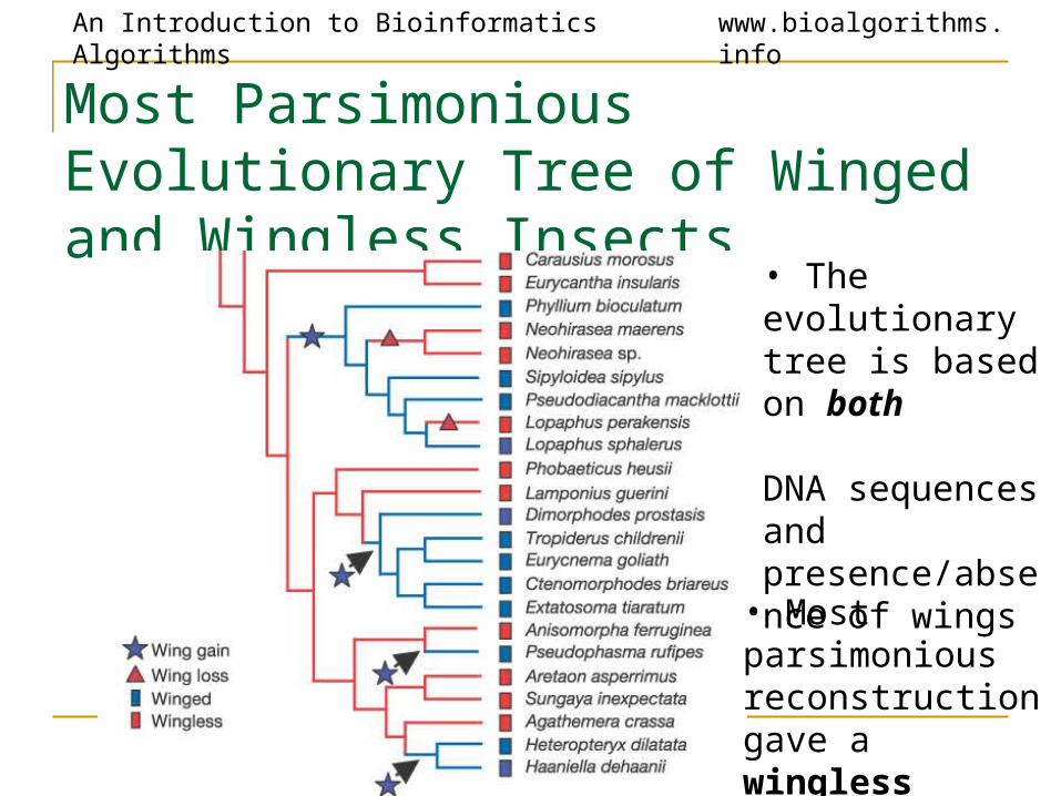
Most Parsimonious Evolutionary Tree of Winged and Wingless Insects
• The evolutionary tree is based on both DNA sequences and presence/absence of wings
• Most parsimonious reconstruction gave a wingless ancestor

An Introduction to Bioinformatics Algorithms www.bioalgorithms.info
Will Wingless Insects Fly Again? • Since the most parsimonious reconstructions
all required the re-invention of wings, it is most likely that wing developmental pathways are conserved in wingless stick insects

An Introduction to Bioinformatics Algorithms www.bioalgorithms.info
Evolutionary Trees
How are these trees built from DNA sequences?

An Introduction to Bioinformatics Algorithms www.bioalgorithms.info
Evolutionary Trees
How are these trees built from DNA sequences?• leaves represent existing species• internal vertices represent ancestors• root represents the oldest evolutionary
ancestor
An Introduction to Bioinformatics Algorithms www.bioalgorithms.info
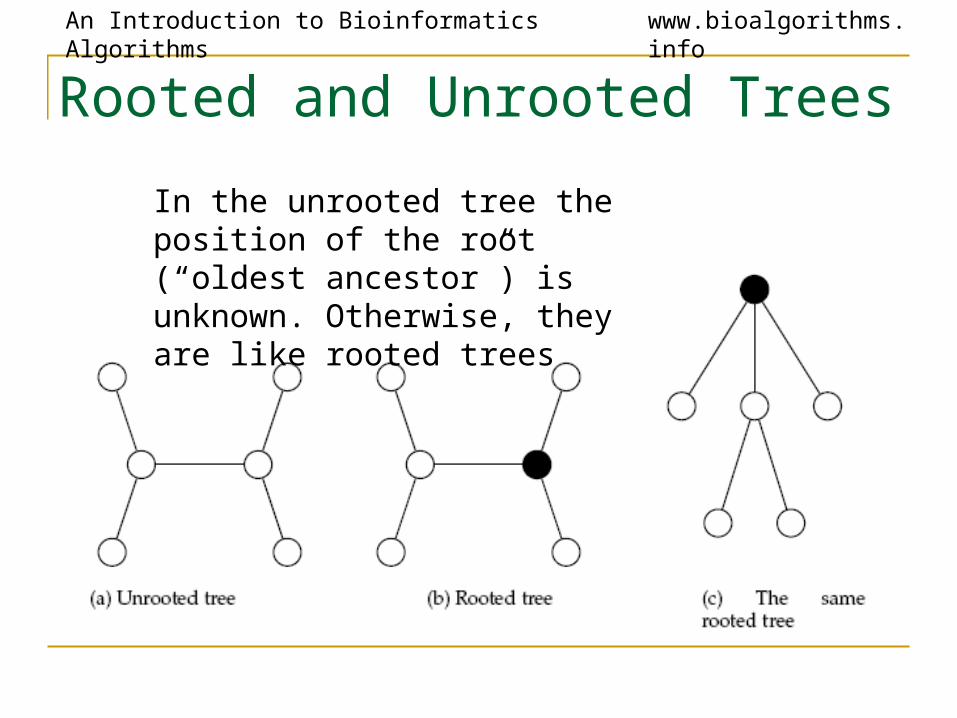
Rooted and Unrooted Trees
In the unrooted tree the position of the root (“oldest ancestor”) is unknown. Otherwise, they are like rooted trees

An Introduction to Bioinformatics Algorithms www.bioalgorithms.info
Distances in Trees
• Edges may have weights reflecting:• Number of mutations on evolutionary path from
one species to another• Time estimate for evolution of one species into
another• In a tree T, we often compute
dij(T) - the length of a path between leaves i and j
dij(T) – tree distance between i and j

An Introduction to Bioinformatics Algorithms www.bioalgorithms.info
Distance in Trees: an Example
d1,4 = 12 + 13 + 14 + 17 + 12 = 68
i
j

An Introduction to Bioinformatics Algorithms www.bioalgorithms.info
Distance Matrix
• Given n species, we can compute the n x n distance matrix Dij
• Dij may be defined as the edit distance between a gene in species i and species j, where the gene of interest is sequenced for all n species.
Dij – edit distance between i and j

An Introduction to Bioinformatics Algorithms www.bioalgorithms.info
Edit Distance vs. Tree Distance• Given n species, we can compute the n x n
distance matrix Dij
• Dij may be defined as the edit distance between a gene in species i and species j, where the gene of interest is sequenced for all n species.
Dij – edit distance between i and j
• Note the difference with
dij(T) – tree distance between i and j

An Introduction to Bioinformatics Algorithms www.bioalgorithms.info
Fitting Distance Matrix
• Given n species, we can compute the n x n distance matrix Dij
• Evolution of these genes is described by a tree that we don’t know.
• We need an algorithm to construct a tree that best fits the distance matrix Dij

An Introduction to Bioinformatics Algorithms www.bioalgorithms.info
Fitting Distance Matrix
• Fitting means Dij = dij(T)
Lengths of path in an (unknown) tree T
Edit distance between species (known)

An Introduction to Bioinformatics Algorithms www.bioalgorithms.info
Reconstructing a 3 Leaved Tree• Tree reconstruction for any 3x3 matrix is
straightforward• We have 3 leaves i, j, k and a center vertex c
Observe:
dic + djc = Dij
dic + dkc = Dik
djc + dkc = Djk

An Introduction to Bioinformatics Algorithms www.bioalgorithms.info
Reconstructing a 3 Leaved Tree (cont’d)
dic + djc = Dij
+ dic + dkc = Dik
2dic + djc + dkc = Dij + Dik
2dic + Djk = Dij + Dik
dic = (Dij + Dik – Djk)/2Similarly,
djc = (Dij + Djk – Dik)/2dkc = (Dki + Dkj – Dij)/2

An Introduction to Bioinformatics Algorithms www.bioalgorithms.info
Trees with > 3 Leaves
• A binary tree with n leaves has 2n-3 edges
• This means fitting a given tree to a distance matrix D requires solving a system of “n choose 2” equations with 2n-3 variables
• This is not always possible to solve for n > 3

An Introduction to Bioinformatics Algorithms www.bioalgorithms.info
Additive Distance Matrices
Matrix D is ADDITIVE if there exists a tree T with dij(T) = Dij
NON-ADDITIVE otherwise

An Introduction to Bioinformatics Algorithms www.bioalgorithms.info
Distance Based Phylogeny Problem• Goal: Reconstruct an evolutionary tree from a
distance matrix• Input: n x n distance matrix Dij
• Output: weighted tree T with n leaves fitting D
• If D is additive, this problem has a solution and there is a simple algorithm to solve it

An Introduction to Bioinformatics Algorithms www.bioalgorithms.info
Using Neighboring Leaves to Construct the Tree
• Find neighboring leaves i and j with parent k• Remove the rows and columns of i and j• Add a new row and column corresponding to k,
where the distance from k to any other leaf m can be computed as:
Dkm = (Dim + Djm – Dij)/2
Compress i and j into k, iterate algorithm for rest of tree
An Introduction to Bioinformatics Algorithms www.bioalgorithms.info
Finding Neighboring Leaves• To find neighboring leaves we simply select a pair
of closest leaves.
An Introduction to Bioinformatics Algorithms www.bioalgorithms.info
Finding Neighboring Leaves• To find neighboring leaves we simply select a pair of closest leaves.
WRONG

An Introduction to Bioinformatics Algorithms www.bioalgorithms.info
Finding Neighboring Leaves• Closest leaves aren’t necessarily neighbors• i and j are neighbors, but (dij = 13) > (djk = 12)
• Finding a pair of neighboring leaves is
a nontrivial problem!

An Introduction to Bioinformatics Algorithms www.bioalgorithms.info
Neighbor Joining Algorithm• In 1987 Naruya Saitou and Masatoshi Nei
developed a neighbor joining algorithm for phylogenetic tree reconstruction
• Finds a pair of leaves that are close to each other but far from other leaves: implicitly finds a pair of neighboring leaves
• Advantages: works well for additive and other non-additive matrices, it does not have the flawed molecular clock assumption

An Introduction to Bioinformatics Algorithms www.bioalgorithms.info
Degenerate Triples
• A degenerate triple is a set of three distinct elements 1≤i,j,k≤n where Dij + Djk = Dik
• Element j in a degenerate triple i,j,k lies on the evolutionary path from i to k (or is attached to this path by an edge of length 0).

An Introduction to Bioinformatics Algorithms www.bioalgorithms.info
Looking for Degenerate Triples
• If distance matrix D has a degenerate triple i,j,k then j can be “removed” from D thus reducing the size of the problem.
• If distance matrix D does not have a degenerate triple i,j,k, one can “create” a degenerative triple in D by shortening all hanging edges (in the tree).

An Introduction to Bioinformatics Algorithms www.bioalgorithms.info
Shortening Hanging Edges to Produce Degenerate Triples• Shorten all “hanging” edges (edges that
connect leaves) until a degenerate triple is found

An Introduction to Bioinformatics Algorithms www.bioalgorithms.info
Finding Degenerate Triples
• If there is no degenerate triple, all hanging edges are reduced by the same amount δ, so that all pair-wise distances in the matrix are reduced by 2δ.
• Eventually this process collapses one of the leaves (when δ = length of shortest hanging edge), forming a degenerate triple i,j,k and reducing the size of the distance matrix D.
• The attachment point for j can be recovered in the reverse transformations by saving Dij for each collapsed leaf.

An Introduction to Bioinformatics Algorithms www.bioalgorithms.info
Reconstructing Trees for Additive Distance Matrices
An Introduction to Bioinformatics Algorithms www.bioalgorithms.info
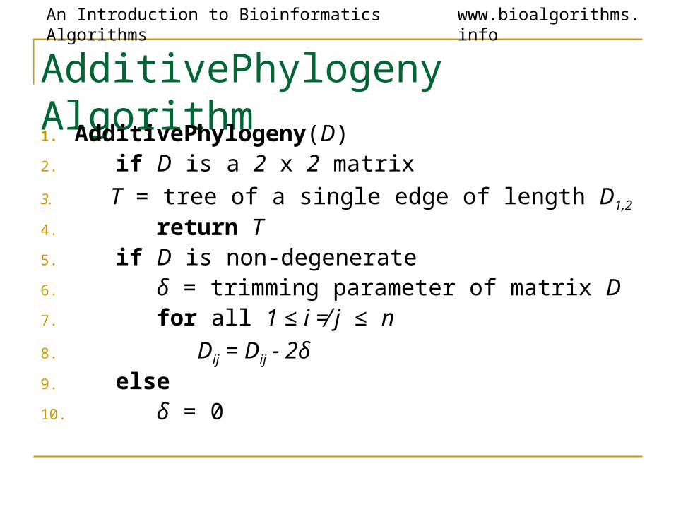
AdditivePhylogeny Algorithm
1. AdditivePhylogeny(D)2. if D is a 2 x 2 matrix3. T = tree of a single edge of length D1,2
4. return T5. if D is non-degenerate6. δ = trimming parameter of matrix D7. for all 1 ≤ i ≠ j ≤ n8. Dij = Dij - 2δ9. else10. δ = 0

An Introduction to Bioinformatics Algorithms www.bioalgorithms.info
AdditivePhylogeny (cont’d)
1. Find a triple i, j, k in D such that Dij + Djk = Dik
2. x = Dij
3. Remove jth row and jth column from D4. T = AdditivePhylogeny(D)5. Add a new vertex v to T at distance x from i to k6. Add j back to T by creating an edge (v,j) of length
07. for every leaf l in T8. if distance from l to v in the tree ≠ Dl,j
9. output “matrix is not additive”10. return11. Extend all “hanging” edges by length δ12. return T
An Introduction to Bioinformatics Algorithms www.bioalgorithms.info
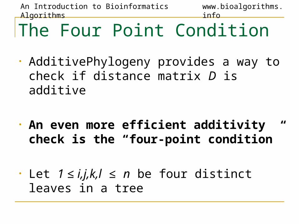
The Four Point Condition
• AdditivePhylogeny provides a way to check if distance matrix D is additive
• An even more efficient additivity check is the “four-point condition”
• Let 1 ≤ i,j,k,l ≤ n be four distinct leaves in a tree

An Introduction to Bioinformatics Algorithms www.bioalgorithms.info
The Four Point Condition (cont’d)
Compute: 1. Dij + Dkl, 2. Dik + Djl, 3. Dil + Djk
1
2 3
2 and 3 represent the same number: the length of all edges + the middle edge (it is counted twice)
1 represents a smaller number: the length of all edges – the middle edge
An Introduction to Bioinformatics Algorithms www.bioalgorithms.info
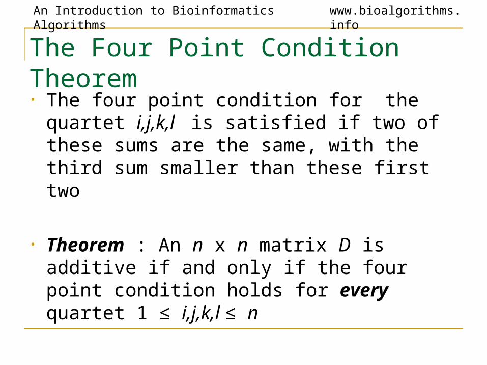
The Four Point Condition Theorem• The four point condition for the quartet i,j,k,l
is satisfied if two of these sums are the same, with the third sum smaller than these first two
• Theorem : An n x n matrix D is additive if and only if the four point condition holds for every quartet 1 ≤ i,j,k,l ≤ n

An Introduction to Bioinformatics Algorithms www.bioalgorithms.info
Least Squares Distance Phylogeny Problem• If the distance matrix D is NOT additive, then we look for a
tree T that approximates D the best:
Squared Error : ∑i,j (dij(T) – Dij)2
• Squared Error is a measure of the quality of the fit between distance matrix and the tree: we want to minimize it.
• Least Squares Distance Phylogeny Problem: finding the best approximation tree T for a non-additive matrix D (NP-hard).

An Introduction to Bioinformatics Algorithms www.bioalgorithms.info
UPGMA: Unweighted Pair Group Method with Arithmetic Mean• UPGMA is a clustering algorithm that:
• computes the distance between clusters using average pairwise distance
• assigns a height to every vertex in the tree, effectively assuming the presence of a molecular clock and dating every vertex

An Introduction to Bioinformatics Algorithms www.bioalgorithms.info
UPGMA’s Weakness
• The algorithm produces an ultrametric tree : the distance from the root to any leaf is the same
• UPGMA assumes a constant molecular clock: all species represented by the leaves in the tree are assumed to accumulate mutations (and thus evolve) at the same rate. This is a major pitfalls of UPGMA.

An Introduction to Bioinformatics Algorithms www.bioalgorithms.info
UPGMA’s Weakness: Example
2
3
41
1 4 32
Correct treeUPGMA

An Introduction to Bioinformatics Algorithms www.bioalgorithms.info
Clustering in UPGMAGiven two disjoint clusters Ci, Cj of sequences,
1
dij = ––––––––– {p Ci, q Cj}dpq
|Ci| |Cj|
Note that if Ck = Ci Cj, then distance to another cluster Cl is:
dil |Ci| + djl |Cj|
dkl = ––––––––––––––
|Ci| + |Cj|

An Introduction to Bioinformatics Algorithms www.bioalgorithms.info
UPGMA Algorithm
Initialization:
Assign each xi to its own cluster Ci
Define one leaf per sequence, each at height 0
Iteration:
Find two clusters Ci and Cj such that dij is min
Let Ck = Ci Cj
Add a vertex connecting Ci, Cj and place it at height dij /2
Delete Ci and Cj
Termination:
When a single cluster remains

An Introduction to Bioinformatics Algorithms www.bioalgorithms.info
Examplev w x y z
v 0 6 8 8 8
w 0 8 8 8
x 0 4 4
y 0 2
z 0
y zxwv
1
2
3
4
v w x yz
v 0 6 8 8
w 0 8 8
x 0 4
yz 0
v w xyz
v 0 6 8
w 0 8
xyz 0
vw xyz
vw 0 8
xyz 0

An Introduction to Bioinformatics Algorithms www.bioalgorithms.info
UPGMA Algorithm (cont’d)
1 4
3 2 5
1 4 2 3 5

An Introduction to Bioinformatics Algorithms www.bioalgorithms.info
Alignment Matrix vs. Distance Matrix
Sequence a gene of length m nucleotides in n species to generate an…
n x m alignment matrix
n x n distance matrix
CANNOT be transformed back into alignment matrix because information was lost on the forward transformation
Transform into…

An Introduction to Bioinformatics Algorithms www.bioalgorithms.info
Character-Based Tree Reconstruction • Better technique:
• Character-based reconstruction algorithms use the n x m alignment matrix
(n = # species, m = #characters)
directly instead of using distance matrix. • GOAL: determine what character strings at
internal nodes would best explain the character strings for the n observed species
An Introduction to Bioinformatics Algorithms www.bioalgorithms.info
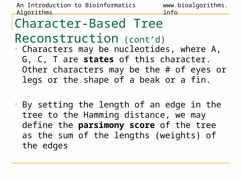
Character-Based Tree Reconstruction (cont’d)• Characters may be nucleotides, where A, G,
C, T are states of this character. Other characters may be the # of eyes or legs or the shape of a beak or a fin.
• By setting the length of an edge in the tree to the Hamming distance, we may define the parsimony score of the tree as the sum of the lengths (weights) of the edges

An Introduction to Bioinformatics Algorithms www.bioalgorithms.info
Parsimony Approach to Evolutionary Tree Reconstruction
• Applies Occam’s razor principle to identify the simplest explanation for the data
• Assumes observed character differences resulted from the fewest possible mutations
• Seeks the tree that yields lowest possible parsimony score - sum of cost of all mutations found in the tree

An Introduction to Bioinformatics Algorithms www.bioalgorithms.info
Parsimony and Tree Reconstruction

An Introduction to Bioinformatics Algorithms www.bioalgorithms.info
Character-Based Tree Reconstruction (cont’d)

An Introduction to Bioinformatics Algorithms www.bioalgorithms.info
Small Parsimony Problem
• Input: Tree T with each leaf labeled by an m-character string.
• Output: Labeling of internal vertices of the tree T minimizing the parsimony score.
• We can assume that every leaf is labeled by a single character, because the characters in the string are independent.

An Introduction to Bioinformatics Algorithms www.bioalgorithms.info
Weighted Small Parsimony Problem• A more general version of Small Parsimony
Problem• Input includes a k * k scoring matrix describing
the cost of transformation of each of k states into another one
• For Small Parsimony problem, the scoring matrix is based on Hamming distance
dH(v, w) = 0 if v=w
dH(v, w) = 1 otherwise

An Introduction to Bioinformatics Algorithms www.bioalgorithms.info
Scoring Matrices
A T G C
A 0 1 1 1
T 1 0 1 1
G 1 1 0 1
C 1 1 1 0
A T G C
A 0 3 4 9
T 3 0 2 4
G 4 2 0 4
C 9 4 4 0
Small Parsimony Problem Weighted Parsimony Problem

An Introduction to Bioinformatics Algorithms www.bioalgorithms.info
Unweighted vs. Weighted
Small Parsimony Scoring Matrix:
A T G C
A 0 1 1 1
T 1 0 1 1
G 1 1 0 1
C 1 1 1 0
Small Parsimony Score:5

An Introduction to Bioinformatics Algorithms www.bioalgorithms.info
Unweighted vs. Weighted
Weighted Parsimony Scoring Matrix:
A T G C
A 0 3 4 9
T 3 0 2 4
G 4 2 0 4
C 9 4 4 0
Weighted Parsimony Score: 22

An Introduction to Bioinformatics Algorithms www.bioalgorithms.info
Weighted Small Parsimony Problem: Formulation
• Input: Tree T with each leaf labeled by elements of a k-letter alphabet and a k x k scoring matrix (ij)
• Output: Labeling of internal vertices of the tree T minimizing the weighted parsimony score

An Introduction to Bioinformatics Algorithms www.bioalgorithms.info
Sankoff Algorithm: Dynamic Programming
• Calculate and keep track of a score for every possible label at each vertex
• st(v) = minimum parsimony score of the subtree rooted at vertex v if v has character t
• The score at each vertex is based on scores of its children:• st(parent) = mini {si( left child ) + i, t} +
minj {sj( right child ) + j, t}

An Introduction to Bioinformatics Algorithms www.bioalgorithms.info
Sankoff’s Algorithm
• Check children’s every vertex and determine the minimum between them
• An example
An Introduction to Bioinformatics Algorithms www.bioalgorithms.info
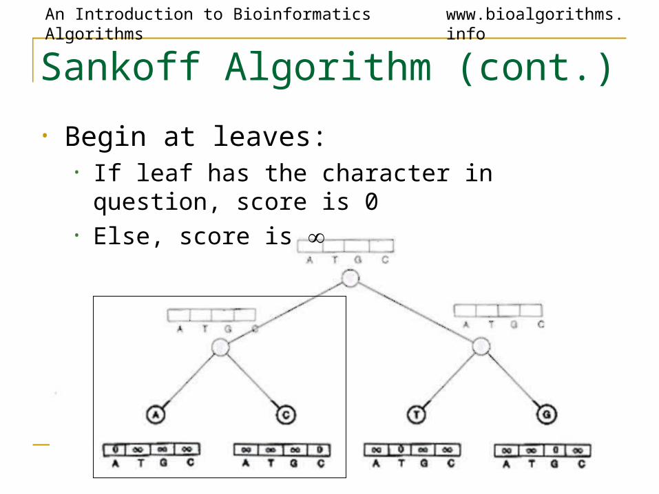
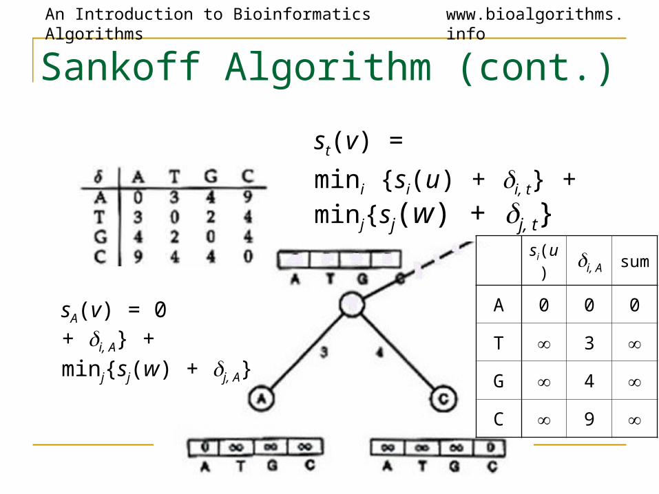
Sankoff Algorithm (cont.)
• Begin at leaves:• If leaf has the character in question, score is 0• Else, score is
An Introduction to Bioinformatics Algorithms www.bioalgorithms.info
Sankoff Algorithm (cont.)
st(v) =
mini {si(u) + i, t} + minj{sj(w) + j, t}
sA(v) = mini{si(u) + i, A} + minj{sj(w) + j, A}
si(u) i, A sum
A 0 0 0
T 3
G 4
C 9
sA(v) = 0

An Introduction to Bioinformatics Algorithms www.bioalgorithms.info
Sankoff Algorithm (cont.)
st(v) =
mini {si(u) + i, t} + minj{sj(w) + j, t}
sA(v) = mini{si(u) + i, A} + minj{sj(w) + j, A}
sj(u) j, A sum
A 0
T 3
G 4
C 0 9 9
+ 9 = 9sA(v) = 0
An Introduction to Bioinformatics Algorithms www.bioalgorithms.info
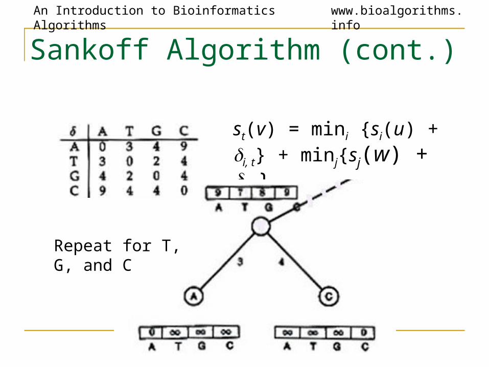
Sankoff Algorithm (cont.)
st(v) = mini {si(u) + i, t} + minj{sj(w) + j, t}
Repeat for T, G, and C

An Introduction to Bioinformatics Algorithms www.bioalgorithms.info
Sankoff Algorithm (cont.)
Repeat for right subtree

An Introduction to Bioinformatics Algorithms www.bioalgorithms.info
Sankoff Algorithm (cont.)
Repeat for root

An Introduction to Bioinformatics Algorithms www.bioalgorithms.info
Sankoff Algorithm (cont.)
Smallest score at root is minimum weighted parsimony score In this case, 9 –
so label with T

An Introduction to Bioinformatics Algorithms www.bioalgorithms.info
Sankoff Algorithm: Traveling down the Tree
• The scores at the root vertex have been computed by going up the tree
• After the scores at root vertex are computed the Sankoff algorithm moves down the tree and assign each vertex with optimal character.

An Introduction to Bioinformatics Algorithms www.bioalgorithms.info
Sankoff Algorithm (cont.)
9 is derived from 7 + 2
So left child is T,
And right child is T

An Introduction to Bioinformatics Algorithms www.bioalgorithms.info
Sankoff Algorithm (cont.)
And the tree is thus labeled…

An Introduction to Bioinformatics Algorithms www.bioalgorithms.info
Fitch’s Algorithm
• Solves Small Parsimony problem• Assigns a set of letter to every vertex in the
tree.• If the two children’s sets of character overlap,
it’s the common set of them• If not, it’s the combined set of them.

An Introduction to Bioinformatics Algorithms www.bioalgorithms.info
Fitch’s Algorithm: An Example
a
a
a
a
a
a
c
c
{t,a}
c
t
t
t
{t,a}
a
{a,c}
{a,c}a
a
a
aa tc
An example:

An Introduction to Bioinformatics Algorithms www.bioalgorithms.info
Fitch Algorithm
1) Assign a set of possible letters to every vertex, traversing the tree from leaves to root
• Each node’s set is the combination of its children’s sets (leaves contain their label)
• If the node has a left child labeled {A, C} and a right child labeled {A, T}, the node will be given the set {A} – intersection of labels
• If the node has a left child labeled {A, C} and a right child labeled {G}, the node will be given the set {A, C, G} – union of labels
An Introduction to Bioinformatics Algorithms www.bioalgorithms.info
Fitch Algorithm (cont.)
2) Assign labels to each vertex, traversing the tree from root to leaves
• Assign root arbitrarily from its set of letters• For all other vertices, if its parent’s label is in
its set of letters, assign it its parent’s label• Else, choose an arbitrary letter from its set as
its label

An Introduction to Bioinformatics Algorithms www.bioalgorithms.info
Fitch Algorithm (cont.)

An Introduction to Bioinformatics Algorithms www.bioalgorithms.info
Fitch vs. Sankoff
• Both have an O(nk) runtime
• Are they actually different?
• Let’s compare …

An Introduction to Bioinformatics Algorithms www.bioalgorithms.info
Fitch
As seen previously:

An Introduction to Bioinformatics Algorithms www.bioalgorithms.info
Comparison of Fitch and Sankoff• As seen earlier, the scoring matrix for the Fitch
algorithm is merely:
• So let’s do the same problem using Sankoff algorithm and this scoring matrix
A T G C
A 0 1 1 1
T 1 0 1 1
G 1 1 0 1
C 1 1 1 0
An Introduction to Bioinformatics Algorithms www.bioalgorithms.info
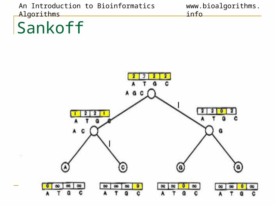
Sankoff

An Introduction to Bioinformatics Algorithms www.bioalgorithms.info
Sankoff vs. Fitch• The Sankoff algorithm gives the same set of
optimal labels as the Fitch algorithm• For Sankoff algorithm, character t is optimal for
vertex v if st(v) = min1<i<ksi(v)• Denote the set of optimal letters at vertex v as S(v)
• If S(left child) and S(right child) overlap, S(parent) is the intersection
• Else it’s the union of S(left child) and S(right child) • This is also the Fitch recurrence
• The two algorithms are identical

An Introduction to Bioinformatics Algorithms www.bioalgorithms.info
Large Parsimony Problem
• Input: An n x m matrix M describing n species, each represented by an m-character string
• Output: A tree T with n leaves labeled by the n rows of matrix M, and a labeling of the internal vertices such that the parsimony score is minimized over all possible trees and all possible labelings of internal vertices

An Introduction to Bioinformatics Algorithms www.bioalgorithms.info
Large Parsimony Problem (cont.)• Possible search space is huge, especially as
n increases• (2n – 3)!! possible rooted trees• (2n – 5)!! possible unrooted trees
• Problem is NP-complete• Exhaustive search only possible w/ small n(< 10)
• Hence, branch and bound or heuristics used

An Introduction to Bioinformatics Algorithms www.bioalgorithms.info
Nearest Neighbor InterchangeA Greedy Algorithm• A Branch Swapping algorithm• Only evaluates a subset of all possible trees• Defines a neighbor of a tree as one
reachable by a nearest neighbor interchange• A rearrangement of the four subtrees defined by
one internal edge• Only three different rearrangements per edge

An Introduction to Bioinformatics Algorithms www.bioalgorithms.info
Nearest Neighbor Interchange (cont.)

An Introduction to Bioinformatics Algorithms www.bioalgorithms.info
Nearest Neighbor Interchange (cont.)• Start with an arbitrary tree and check its
neighbors• Move to a neighbor if it provides the best
improvement in parsimony score• No way of knowing if the result is the most
parsimonious tree• Could be stuck in local optimum
An Introduction to Bioinformatics Algorithms www.bioalgorithms.info
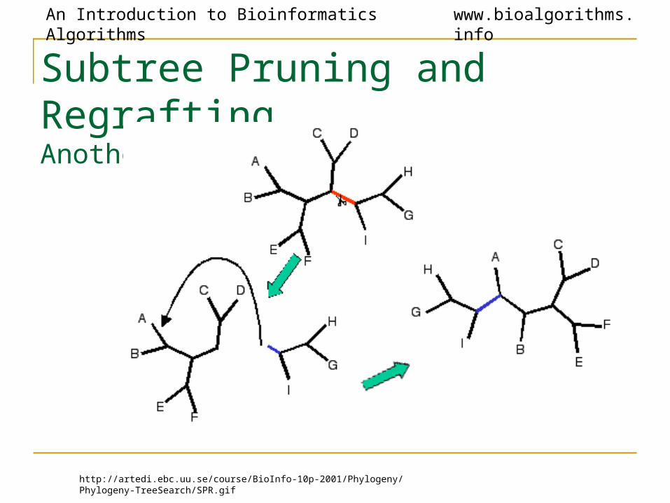
Subtree Pruning and RegraftingAnother Branch Swapping Algorithm
http://artedi.ebc.uu.se/course/BioInfo-10p-2001/Phylogeny/Phylogeny-TreeSearch/SPR.gif

An Introduction to Bioinformatics Algorithms www.bioalgorithms.info
Tree Bisection and Reconnection Another Branch Swapping Algorithm

An Introduction to Bioinformatics Algorithms www.bioalgorithms.info
Homoplasy• Given:
• 1: CAGCAGCAG• 2: CAGCAGCAG• 3: CAGCAGCAGCAG• 4: CAGCAGCAG• 5: CAGCAGCAG• 6: CAGCAGCAG• 7: CAGCAGCAGCAG
• Most would group 1, 2, 4, 5, and 6 as having evolved from a common ancestor, with a single mutation leading to the presence of 3 and 7

An Introduction to Bioinformatics Algorithms www.bioalgorithms.info
Homoplasy
• But what if this was the real tree?
An Introduction to Bioinformatics Algorithms www.bioalgorithms.info
Homoplasy
• 6 evolved separately from 4 and 5, but parsimony would group 4, 5, and 6 together as having evolved from a common ancestor
• Homoplasy: Independent (or parallel) evolution of same/similar characters
• Parsimony minimizes homoplasy, so if homoplasy is common, parsimony may give wrong results

An Introduction to Bioinformatics Algorithms www.bioalgorithms.info
Contradicting Characters• An evolutionary tree is more likely to be
correct when it is supported by multiple characters, as seen below
Lizard
Frog
Human
Dog
MAMMALIAHairSingle bone in lower jawLactationetc.
Note: In this case, tails are homoplasic

An Introduction to Bioinformatics Algorithms www.bioalgorithms.info
Problems with Parsimony
• Important to keep in mind that reliance on purely one method for phylogenetic analysis provides incomplete picture
• When different methods (parsimony, distance-based, etc.) all give same result, more likely that the result is correct
An Introduction to Bioinformatics Algorithms www.bioalgorithms.info
Alu Repeats • Alu repeats are most common repeats in human
genome (about 300 bp long)• About 1 million Alu elements make up 10% of the
human genome• They are retrotransposons
• they don’t code for protein but copy themselves into RNA and then back to DNA via reverse transcriptase
• Alu elements have been called “selfish” because their only function seems to be to make more copies of themselves
An Introduction to Bioinformatics Algorithms www.bioalgorithms.info
What Makes Alu Elements Important?• Alu elements began to replicate 60 million
years ago. Their evolution can be used as a fossil record of primate and human history
• Alu insertions are sometimes disruptive and can result in genetic disorders
• Alu mediated recombination can cause cancer
• Alu insertions can be used to determine genetic distances between human populations and human migratory history

An Introduction to Bioinformatics Algorithms www.bioalgorithms.info
Minimum Spanning Trees• The first algorithm for finding a MST
was developed in 1926 by Otakar Borůvka. Its purpose was to minimize the cost of electrical coverage in Bohemia.
• The Problem• Connect all of the cities but use the
least amount of electrical wire possible. This reduces the cost.
• We will see how building a MST can be used to study evolution of Alu repeats

An Introduction to Bioinformatics Algorithms www.bioalgorithms.info
What is a Minimum Spanning What is a Minimum Spanning Tree?Tree?• A Minimum
Spanning Tree of a graph
--connects all the vertices in the graph and
--minimizes the sum of edges in the tree among all spanning trees

An Introduction to Bioinformatics Algorithms www.bioalgorithms.info
How can we find a MST?How can we find a MST?
• Prim algorithm (greedy)• Start from a tree T with a single vertex• Add the shortest edge connecting a vertex in
T to a vertex not in T, growing the tree T• This is repeated until every vertex is in T
• Prim algorithm can be implemented in O(m logm) time (m is the number of edges).

An Introduction to Bioinformatics Algorithms www.bioalgorithms.info
Prim’s Algorithm ExamplePrim’s Algorithm Example

An Introduction to Bioinformatics Algorithms www.bioalgorithms.info
Why Prim Algorithm Constructs Why Prim Algorithm Constructs Minimum Spanning Tree? Minimum Spanning Tree?
• Proof:• This proof applies to a graph with distinct
lengths of edges• Let e be any edge that Prim algorithm
chose to connect two sets of nodes. Suppose that Prim’s algorithm is flawed and it is cheaper to connect the two sets of nodes via some other edge f
• Notice that since Prim algorithm selected edge e we know that cost(e) < cost(f)
• By connecting the two sets via edge f, the cost of connecting the two vertices has gone up by exactly cost(f) – cost(e)
• The contradiction is that edge e does not belong in the MST yet the MST can’t be formed without using edge e

An Introduction to Bioinformatics Algorithms www.bioalgorithms.info
An Alu Element
• SINEs are flanked by short direct repeat sequences and are transcribed by RNA Polymerase III

An Introduction to Bioinformatics Algorithms www.bioalgorithms.info
Alu Subfamilies

An Introduction to Bioinformatics Algorithms www.bioalgorithms.info
The Biological Story: Alu Evolution

An Introduction to Bioinformatics Algorithms www.bioalgorithms.info
Alu Evolution

An Introduction to Bioinformatics Algorithms www.bioalgorithms.info
Alu Evolution: The Master Alu Theory

An Introduction to Bioinformatics Algorithms www.bioalgorithms.info
Alu Evolution: Alu Master Theory Proven Wrong

An Introduction to Bioinformatics Algorithms www.bioalgorithms.info
Minimum Spanning Tree As An Evolutionary Tree

An Introduction to Bioinformatics Algorithms www.bioalgorithms.info
Alu Evolution: Minimum Spanning Tree vs. Phylogenetic Tree• A timeline of Alu subfamily evolution would give
useful information• Problem - building a traditional phylogenetic tree
with Alu subfamilies will not describe Alu evolution accurately
• Why can’t a meaningful typical phylogenetic tree of Alu subfamilies be constructed?• When constructing a typical phylogenetic tree, the
input is made up of leaf nodes, but no internal nodes
• Alu subfamilies may be either internal or external nodes of the evolutionary tree because Alu subfamilies that created new Alu subfamilies are themselves still present in the genome. Traditional phylogenetic tree reconstruction methods are not applicable since they don’t allow for the inclusion of such internal nodes
An Introduction to Bioinformatics Algorithms www.bioalgorithms.info
Constructing MST for Alu Evolution• Building an evolutionary tree using an MST will allow for the inclusion
of internal nodes• Define the length between two subfamilies as the Hamming distance
between their sequences• Root the subfamily with highest average divergence from its consensus
sequence (the oldest subfamily), as the root• It takes ~4 million years for 1% of sequence divergence between
subfamilies to emerge, this allows for the creation of a timeline of Alu evolution to be created
• Why an MST is useful as an evolutionary tree in this case• The less the Hamming distance (edge weight) between two subfamilies,
the more likely that they are directly related• An MST represents a way for Alu subfamilies to have evolved minimizing
the sum of all the edge weights (total Hamming distance between all Alu subfamilies) which makes it the most parsimonious way and thus the most likely way for the evolution of the subfamilies to have occurred.

An Introduction to Bioinformatics Algorithms www.bioalgorithms.info
MST As An Evolutionary Tree

An Introduction to Bioinformatics Algorithms www.bioalgorithms.info
Sources• http://www.math.tau.ac.il/~rshamir/ge/02/scribes/lec01.pdf• Serafim Batzoglou (UPGMA slides)
http://www.stanford.edu/class/cs262/Slides• Watkins, W.S., Rogers A.R., Ostler C.T., Wooding, S., Bamshad M. J.,
Brassington A.E., Carroll M.L., Nguyen S.V., Walker J.A., Prasas, R., Reddy P.G., Das P.K., Batzer M.A., Jorde, L.B.: Genetic Variation Among World Populations: Inferences From 100 Alu Insertion Polymorphisms


