Molecular Magnetic Properties Workshop on Theoretical Chemistry Mariapfarr, Salzburg, Austria February 14–17, 2006 Trygve Helgaker Department of Chemistry, University of Oslo, Norway Overview • The electronic Hamiltonian in an electromagnetic field • The calculation of molecular magnetic properties 1
Transcript
Molecular Magnetic Properties
Workshop on Theoretical Chemistry
Mariapfarr, Salzburg, Austria
February 14–17, 2006
Trygve Helgaker
Department of Chemistry, University of Oslo, Norway
Overview
• The electronic Hamiltonian in an electromagnetic field
• The calculation of molecular magnetic properties
1
Nonrelativistic electronic Hamiltonian in an electromagnetic field
• classical mechanics of particles
– Newtonian mechanics (1687)
– Lagrangian mechanics (1788)
– Hamiltonian mechanics (1833)
• electromagnetic fields
– Maxwell’s equations (1864)
– scalar and vector potentials
– gauge transformations
• spin-free electron in an electromagnetic field
– the Lagrangian and the Hamiltonian of a particle in an electromagnetic field
– the Schrodinger Hamiltonian (1925)
• spinning electron in an electromagnetic field
– the Dirac equation and electron spin (1928)
– the Schrodinger–Pauli Hamiltonian (Pauli, 1927)
2
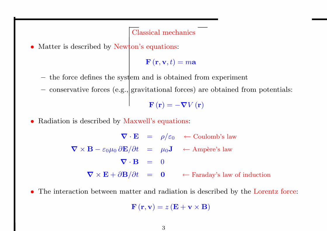
Classical mechanics
• Matter is described by Newton’s equations:
F (r,v, t) = ma
– the force defines the system and is obtained from experiment
– conservative forces (e.g., gravitational forces) are obtained from potentials:
F (r) = −∇V (r)
• Radiation is described by Maxwell’s equations:
∇ ·E = ρ/ε0 ← Coulomb’s law
∇ ×B− ε0µ0 ∂E/∂t = µ0J ← Ampere’s law
∇ ·B = 0
∇ ×E + ∂B/∂t = 0 ← Faraday’s law of induction
• The interaction between matter and radiation is described by the Lorentz force:
F (r,v) = z (E + v×B)
3
Lagrangian mechanics: the principle of least action
• For a system of n degrees of freedom, there are
– n generalized coordinates qi in configuration space
– n generalized velocities qi
• The principle of least action (Hamilton’s principle):
For each system, there exists a Lagrangian L(qi, qi, t) such that the action
integral
S =
Z t2
t1
L(qi, qi, t) dt
assumes an extremum along the trajectory in configuration space taken by
the system.
t1 t2
qiHt1L
qiHt2L
4
Lagrange’s equations
• From the principle of least action, we obtain
δS = δ
Z t2
t1
L(qi, qi, t) dt =
Z t2
t1
„∂L
∂qi
δqi +∂L
∂qi
δqi
«
dt
=
Z t2
t1
»∂L
∂qi
δqi −
„d
dt
∂L
∂qi
«
δqi
–
dt = 0
• We conclude that the Lagrangian satisfies the following second-order differential
equations (one for each degree of freedom):
ddt
∂L∂qi
=∂L∂qi
← Lagrange’s equations of motion
– the Lagrangian defines the system and is determined so that it reproduces the
equations of motion consistent with experiment.
– Lagrange’s equations preserve their form in any coordinate system.
• A more general formulation than the Newtonian one:
– unified description of matter and fields (Newton’s and Maxwell’s equations)
– springboard for quantum mechanics
5
Arbitrariness of the Lagrangian and gauge transformations
• The scalar Lagrangian is not uniquely defined.
• Assume that the Lagrangian L(q, q, t) satisfies the equations:
d
dt
∂L
∂q=
∂L
∂q.
• Consider now the following transformed Lagrangian where the arbitrary gauge
function f (q, t) is independent of the velocity q:
L′ (q, q, t) = L (q, q, t) +d
dtf (q, t).
• The new Lagrangian satisfies the same equations of motion as the old one:
d
dt
∂L′
∂q=
d
dt
∂L
∂q+
d
dt
∂
∂q
„∂f
∂qq +
∂f
∂t
«
=∂L
∂q+
d
dt
∂f
∂q=
∂
∂q
„
L +d
dtf
«
=∂L′
∂q.
• This is an example of a gauge transformation.
6
Conservative systems
• The Lagrangian of a particle in a conservative field may be written as
L = T (q, q)| z
kinetic energy
− V (q)| z
potential energy
• The Lagrangian is thus easily set up for any conservative system, in any
convenient coordinate system.
• Example: Assuming a Cartesian coordinate system
L =1
2mv2 − V (r) ,
we find that Lagrange’s equations immediately reduce to Newton’s equations:
d
dt
∂L
∂v=
∂L
∂r⇒
d
dtmv = −∇V (r) ⇒ ma = F.
• For particles in a (nonconservative) electromagnetic field, the Lagrangian can be
cast in similar but slightly different form as discussed later.
7
The energy function
• In Lagrangian mechanics, the energy function is defined as:
h (q, q, t) =∂L
∂qq − L (q, q, t) .
• Assume a conservative Cartesian system with Lagrangian L = 12mv2 − V (r):
h =∂L
∂vv− L =
∂T
∂vv − (T − V ) = 2T − T + V = T + V = total energy
– More generally, h is equal to the total energy if T (q) is quadratic in q and
V (q) is independent of q.
• The energy function h is conserved if L does not depend explicitly on time:
dh
dt= −
∂L
∂t
– Proof:
dh
dt=
d
dt
„∂L
∂qq
«
−dL
dt
=
»„d
dt
∂L
∂q
«
q +∂L
∂qq
–
−
»∂L
∂qq +
∂L
∂qq +
∂L
∂t
–
= −∂L
∂t
8
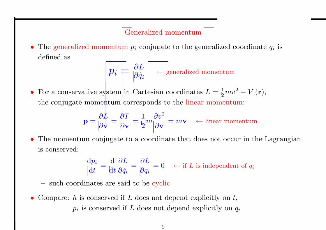
Generalized momentum
• The generalized momentum pi conjugate to the generalized coordinate qi is
defined as
pi =∂L∂qi
← generalized momentum
• For a conservative system in Cartesian coordinates L = 12mv2 − V (r),
the conjugate momentum corresponds to the linear momentum:
p =∂L
∂v=
∂T
∂v=
1
2m
∂v2
∂v= mv ← linear momentum
• The momentum conjugate to a coordinate that does not occur in the Lagrangian
is conserved:
dpi
dt=
d
dt
∂L
∂qi
=∂L
∂qi
= 0 ← if L is independent of qi
– such coordinates are said to be cyclic
• Compare: h is conserved if L does not depend explicitly on t,
pi is conserved if L does not depend explicitly on qi
9
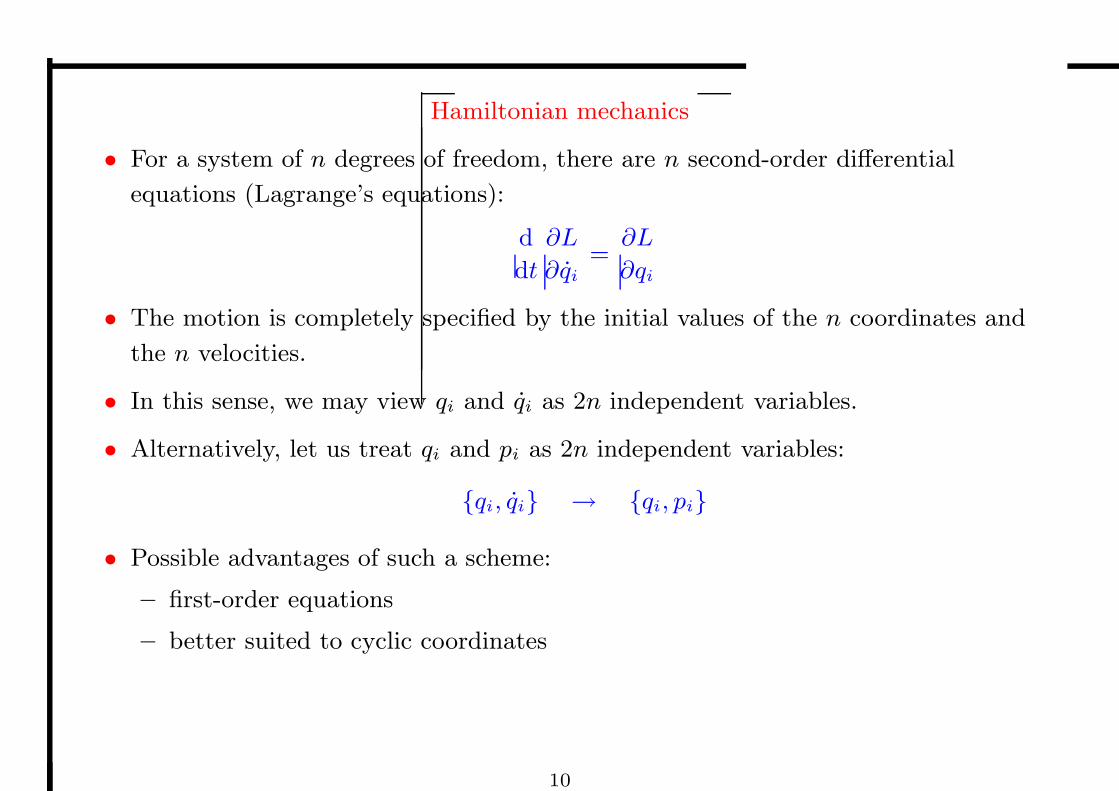
Hamiltonian mechanics
• For a system of n degrees of freedom, there are n second-order differential
equations (Lagrange’s equations):
d
dt
∂L
∂qi
=∂L
∂qi
• The motion is completely specified by the initial values of the n coordinates and
the n velocities.
• In this sense, we may view qi and qi as 2n independent variables.
• Alternatively, let us treat qi and pi as 2n independent variables:
qi, qi → qi, pi
• Possible advantages of such a scheme:
– first-order equations
– better suited to cyclic coordinates
10
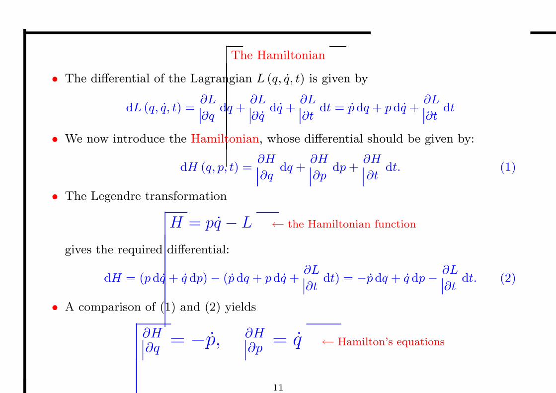
The Hamiltonian
• The differential of the Lagrangian L (q, q, t) is given by
dL (q, q, t) =∂L
∂qdq +
∂L
∂qdq +
∂L
∂tdt = pdq + p dq +
∂L
∂tdt
• We now introduce the Hamiltonian, whose differential should be given by:
dH (q, p, t) =∂H
∂qdq +
∂H
∂pdp +
∂H
∂tdt. (1)
• The Legendre transformation
H = pq − L ← the Hamiltonian function
gives the required differential:
dH = (pdq + q dp)− (p dq + pdq +∂L
∂tdt) = −pdq + q dp−
∂L
∂tdt. (2)
• A comparison of (1) and (2) yields
∂H∂q
= −p, ∂H∂p
= q ← Hamilton’s equations
11
Prescription for setting up the Hamiltonian
1. Choose n generalized coordinates qi.
2. Set up the Lagrangian L (qi, qi, t) such that
d
dt
∂L
∂qi
=∂L
∂qi
(1)
reproduces the equations of motion.
3. Introduce the conjugate momenta
pi =∂L
∂qi
. (2)
4. Construct the Hamiltonian
H =X
i
piqi − L (qi, qi, t) (3)
and invert (2) to express the Hamiltonian H (qi, pi) in terms of qi and pi.
5. Write down Hamilton’s equations of motion:
qi =∂H
∂pi
, pi = −∂H
∂qi
. (4)
12
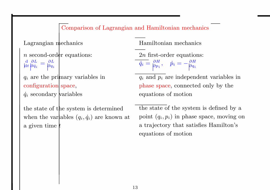
Comparison of Lagrangian and Hamiltonian mechanics
Lagrangian mechanics Hamiltonian mechanics
n second-order equations: 2n first-order equations:ddt
∂L∂qi
= ∂L∂qi
qi = ∂H∂pi
, pi = − ∂H∂qi
qi are the primary variables in
configuration space,
qi secondary variables
qi and pi are independent variables in
phase space, connected only by the
equations of motion
the state of the system is determined
when the variables (qi, qi) are known at
a given time t
the state of the system is defined by a
point (qi, pi) in phase space, moving on
a trajectory that satisfies Hamilton’s
equations of motion
13
Poisson brackets
• The Poisson bracket of two dynamical variables A (q, p, t) and B (q, p, t) is defined
as
[A, B] =X
i
„∂A
∂qi
∂B
∂pi
−∂B
∂qi
∂A
∂pi
«
– the fundamental Poisson brackets among conjugate coordinates and momenta:
[qi, qj ] = 0, [pi, pj ] = 0, [qi, pj ] = δij
• The total time derivatives are given by
dA
dt=
∂A
∂qq +
∂A
∂pp +
∂A
∂t=
∂A
∂q
∂H
∂p−
∂A
∂p
∂H
∂q+
∂A
∂t,
and may therefore be expressed compactly as
dA
dt= [A, H] +
∂A
∂t.
– important special cases:
q = [q, H] , p = [p, H] ,dH
dt=
∂H
∂t
14
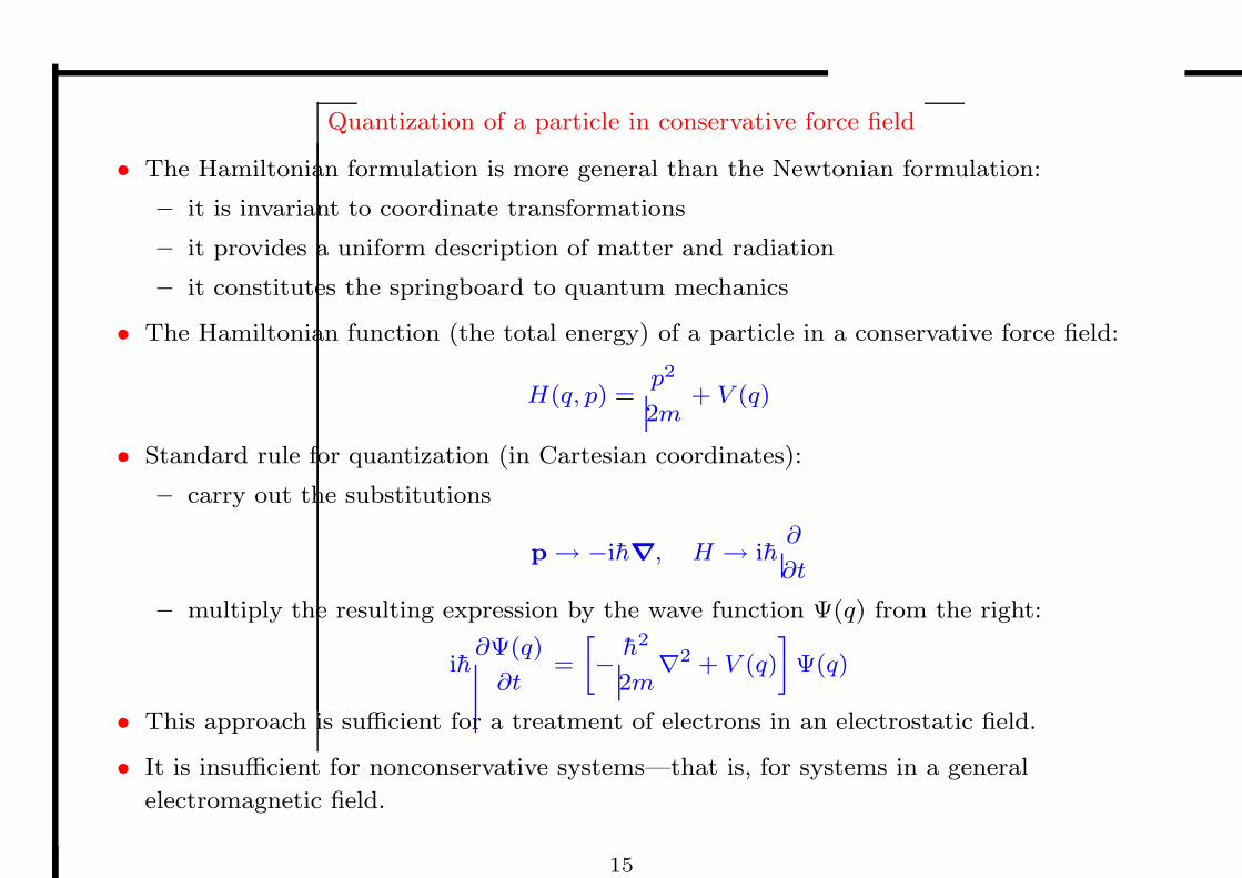
Quantization of a particle in conservative force field
• The Hamiltonian formulation is more general than the Newtonian formulation:
– it is invariant to coordinate transformations
– it provides a uniform description of matter and radiation
– it constitutes the springboard to quantum mechanics
• The Hamiltonian function (the total energy) of a particle in a conservative force field:
H(q, p) =p2
2m+ V (q)
• Standard rule for quantization (in Cartesian coordinates):
– carry out the substitutions
p→ −ih∇, H → ih∂
∂t
– multiply the resulting expression by the wave function Ψ(q) from the right:
ih∂Ψ(q)
∂t=
»
−h2
2m∇2 + V (q)
–
Ψ(q)
• This approach is sufficient for a treatment of electrons in an electrostatic field.
• It is insufficient for nonconservative systems—that is, for systems in a general
electromagnetic field.
15
Review: Hamiltonian mechanics
• In classical Hamiltonian mechanics, a system of particles is described in terms their
positions qi and conjugate momenta pi.
• For each such system, there exists a scalar Hamiltonian function H(qi, pi) such that the
classical equations of motion are given by:
qi =∂H
∂pi
, pi = −∂H
∂qi
(Hamilton’s equations of motion)
• Example: a single particle of mass m in a conservative force field F (q)
– the Hamiltonian function is constructed from a scalar potential:
H(q, p) =p2
2m+ V (q), F (q) = −
∂V (q)
∂q
– Hamilton’s equations are equivalent to Newton’s equations:
q =∂H(q,p)
∂p= p
m
p = −∂H(q,p)
∂q= −
∂V (q)∂q
9=
;⇒ mq = F (q) (Newton’s equations of motion)
• Whereas Newton’s equations of motion are second-order differential equations,
Hamilton’s equations are first-order.
• We must now generalize this approach to particles in an electromagnetic field!
16
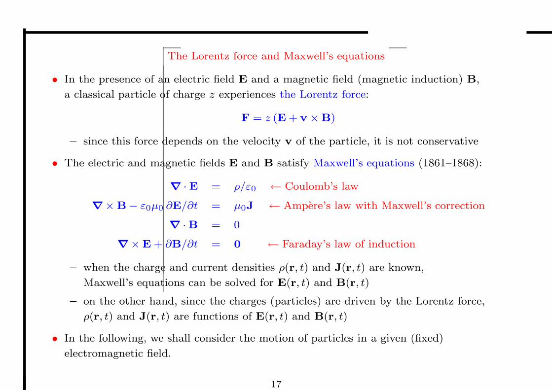
The Lorentz force and Maxwell’s equations
• In the presence of an electric field E and a magnetic field (magnetic induction) B,
a classical particle of charge z experiences the Lorentz force:
F = z (E + v ×B)
– since this force depends on the velocity v of the particle, it is not conservative
• The electric and magnetic fields E and B satisfy Maxwell’s equations (1861–1868):
∇ · E = ρ/ε0 ← Coulomb’s law
∇×B− ε0µ0 ∂E/∂t = µ0J ← Ampere’s law with Maxwell’s correction
∇ ·B = 0
∇×E + ∂B/∂t = 0 ← Faraday’s law of induction
– when the charge and current densities ρ(r, t) and J(r, t) are known,
Maxwell’s equations can be solved for E(r, t) and B(r, t)
– on the other hand, since the charges (particles) are driven by the Lorentz force,
ρ(r, t) and J(r, t) are functions of E(r, t) and B(r, t)
• In the following, we shall consider the motion of particles in a given (fixed)
electromagnetic field.
17
Scalar and vector potentials
• The second, homogeneous pair of Maxwell’s equations involve only E and B:
∇ ·B = 0 (1)
∇×E +∂B
∂t= 0 (2)
1. Equation (1) is satisfied by introducing the vector potential A:
∇ ·B = 0 ⇒ B = ∇×A ← vector potential (3)
2. Inserting Eq. (3) in Eq. (2) and introducing a scalar potential φ, we obtain
∇×
„
E +∂A
∂t
«
= 0 ⇒ E +∂A
∂t= −∇φ ← scalar potential
• The second pair of Maxwell’s equations are thus automatically satisfied by writing
E = −∇φ−∂A
∂tB = ∇×A
• The potentials (φ,A) contain four rather than six components as in (E,B).
• They are obtained by solving the first, inhomogeneous pair of Maxwell’s equations,
which contains ρ and J.
18
Particle in an electromagnetic field
• For a particle in an electromagnetic field, we must set up a Lagrangian such that
d
dt
∂L
∂qi
=∂L
∂qi
reduces to Newton’s equations with the Lorentz force
F = z (E + v ×B) , E = −∇φ−∂A
∂t, B = ∇×A
• This is not a conservative system, for which
L = T − V, Fi = −∂V
∂qi
• Rather, it belongs to a broader class of systems, for which
L = T − U, Fi = −∂U
∂qi
+d
dt
„∂U
∂qi
«
• For a particle subject to the Lorentz force, the generalized potential is given by
U = z (φ− v ·A) ← velocity-dependent potential
and the Lagrangian becomes
L = T − z (φ− v ·A) ← particle in an electromagnetic field
19
Conjugate momentum in an electromagnetic field
• We recall that, for a conservative system described by Lagrangian of the form
L (q, q) = T (q)− V (q) ,
the conjugate momentum in Cartesian coordinates
p =∂L
∂v=
∂T
∂v= mv ≡ π
is equal to the linear (kinetic) momentum π:
p = π ← particle in a conservative field
• By contrast, for a nonconservative system described by Lagrangian
L (q, q) = T (q)− U (q, q) ,
the conjugate and kinetic momenta are no longer the same.
• In particular, for a particle in an electromagnetic field
L = T − z (φ− v ·A)
we obtain
p =∂L
∂v=
∂T
∂v+ zA ⇒ p = π + zA ← particle in an electromagnetic field
20
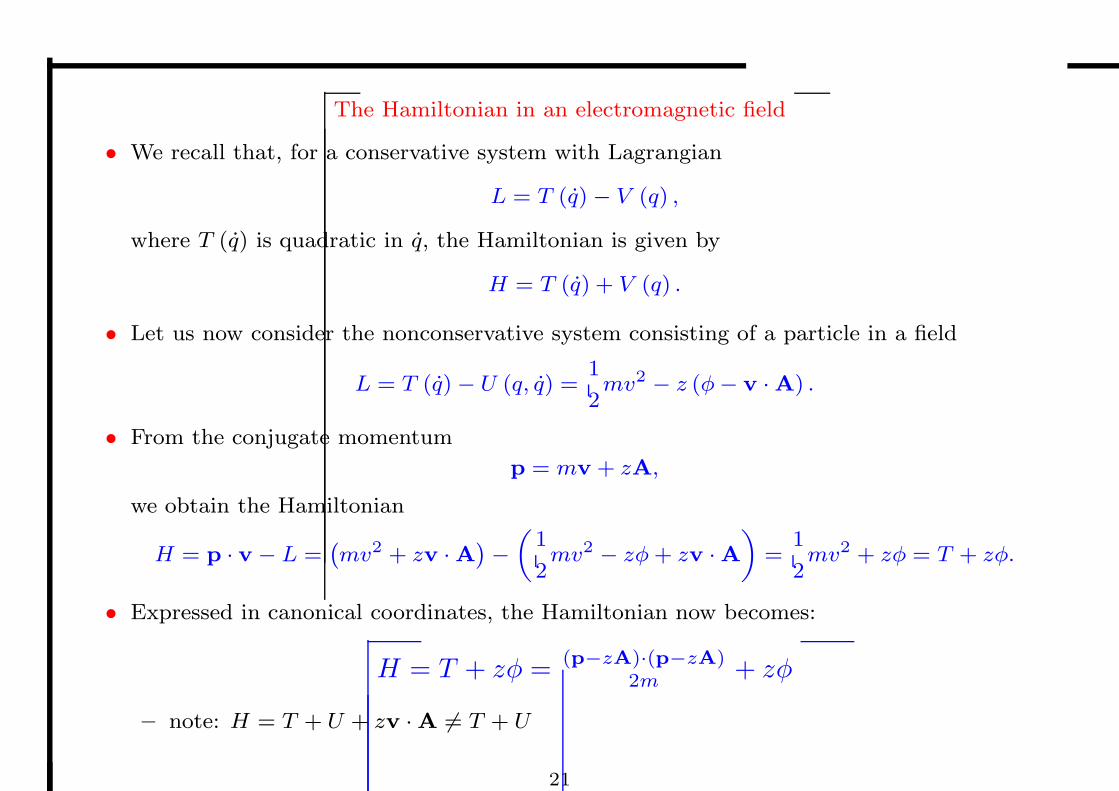
The Hamiltonian in an electromagnetic field
• We recall that, for a conservative system with Lagrangian
L = T (q)− V (q) ,
where T (q) is quadratic in q, the Hamiltonian is given by
H = T (q) + V (q) .
• Let us now consider the nonconservative system consisting of a particle in a field
L = T (q)− U (q, q) =1
2mv2 − z (φ− v ·A) .
• From the conjugate momentum
p = mv + zA,
we obtain the Hamiltonian
H = p · v − L =`mv2 + zv ·A
´−
„1
2mv2 − zφ + zv ·A
«
=1
2mv2 + zφ = T + zφ.
• Expressed in canonical coordinates, the Hamiltonian now becomes:
H = T + zφ = (p−zA)·(p−zA)2m
+ zφ
– note: H = T + U + zv ·A 6= T + U
21
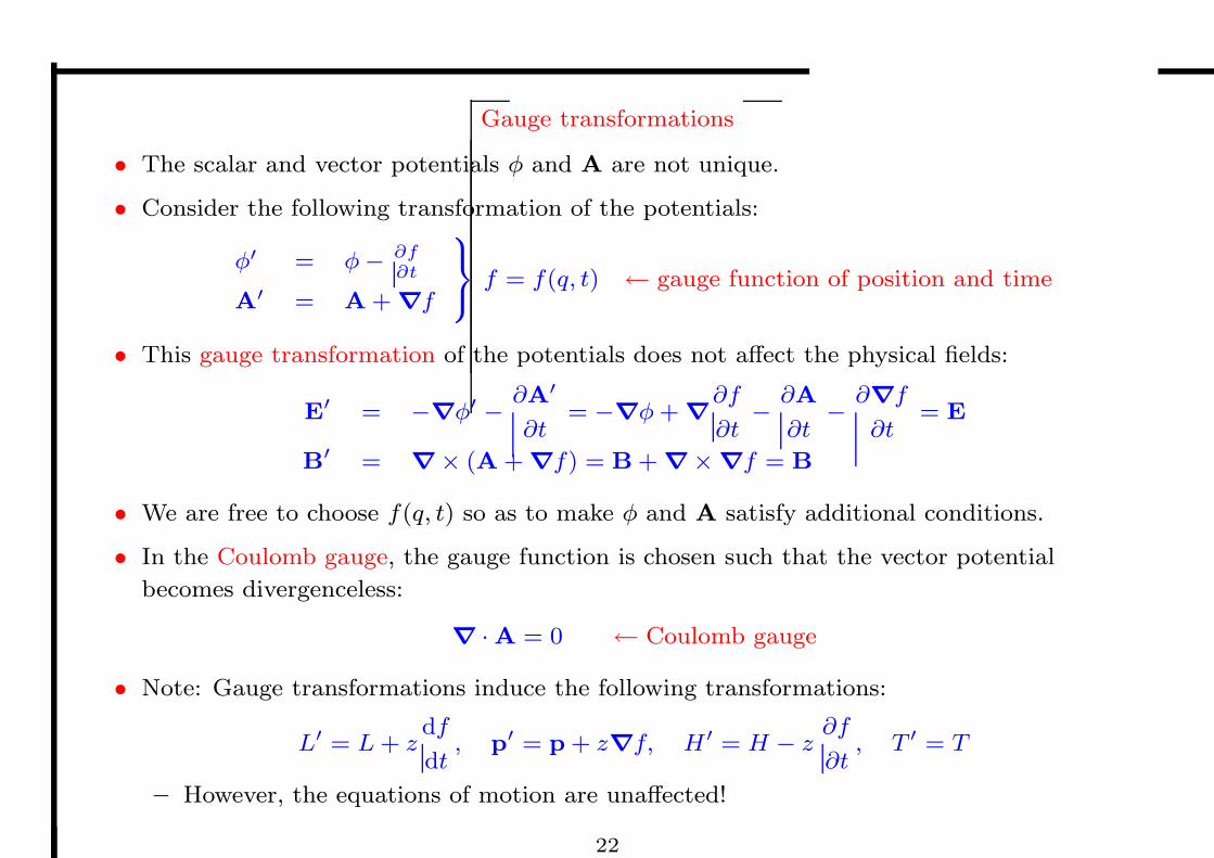
Gauge transformations
• The scalar and vector potentials φ and A are not unique.
• Consider the following transformation of the potentials:
φ′ = φ− ∂f∂t
A′ = A + ∇f
9=
;f = f(q, t) ← gauge function of position and time
• This gauge transformation of the potentials does not affect the physical fields:
E′ = −∇φ′ −∂A′
∂t= −∇φ + ∇
∂f
∂t−
∂A
∂t−
∂∇f
∂t= E
B′ = ∇× (A + ∇f) = B + ∇×∇f = B
• We are free to choose f(q, t) so as to make φ and A satisfy additional conditions.
• In the Coulomb gauge, the gauge function is chosen such that the vector potential
becomes divergenceless:
∇ ·A = 0 ← Coulomb gauge
• Note: Gauge transformations induce the following transformations:
L′ = L + zdf
dt, p′ = p + z∇f, H′ = H − z
∂f
∂t, T ′ = T
– However, the equations of motion are unaffected!
22
Quantization of a particle in an electromagnetic field
• We have now constructed a Hamiltonian function such that Hamilton’s equations are
equivalent to Newton’s equation with the Lorentz force:
qi =∂H
∂pi
& pi = −∂H
∂qi
⇔ ma = z (E + v ×B)
• To this end, we introduced scalar and vector potentials φ and A such that
E = −∇φ−∂A
∂t, B = ∇×A
• In terms of these potentials, the classical Hamiltonian function takes the form
H =π2
2m+ zφ, π = p− zA ← kinetic momentum
• Quantization is now accomplished in the usual manner, by the substitutions
p→ −ih∇, H → ih∂
∂t
• This results in the following time-dependent Schrodinger equation for a particle in an
electromagnetic field:
ih∂Ψ
∂t=
1
2m(−ih∇− zA) · (−ih∇− zA)Ψ + zφ Ψ
23
Electron spin
• According to our previous discussion, the nonrelativistic Hamiltonian for an electron in
an electromagnetic field is given by:
H =π2
2m− eφ, π = −ih∇ + eA
• However, this description ignores a fundamental property of the electron: spin.
• Spin was introduced by Pauli in 1927, to fit experimental observations:
H =(σ · π)2
2m− eφ =
π2
2m+
eh
2mB · σ− eφ
where σ contains three operators, represented by the two-by-two Pauli spin matrices
σx =
0
@0 1
1 0
1
A , σy =
0
@0 −i
i 0
1
A , σz =
0
@1 0
0 −1
1
A
• The Schrodinger equation now becomes a two-component equation0
@
π2
2m− eφ + eh
2mBz
eh2m
(Bx − iBy)
eh2m
(Bx + iBy) π2
2m− eφ− eh
2mBz
1
A
0
@Ψα
Ψβ
1
A = E
0
@Ψα
Ψβ
1
A
– the two components are only coupled in the presence of an external magnetic field
24
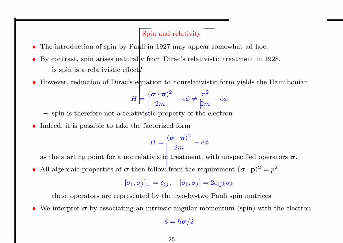
Spin and relativity
• The introduction of spin by Pauli in 1927 may appear somewhat ad hoc.
• By contrast, spin arises naturally from Dirac’s relativistic treatment in 1928.
– is spin is a relativistic effect?
• However, reduction of Dirac’s equation to nonrelativistic form yields the Hamiltonian
H =(σ · π)2
2m− eφ 6=
π2
2m− eφ
– spin is therefore not a relativistic property of the electron
• Indeed, it is possible to take the factorized form
H =(σ · π)2
2m− eφ
as the starting point for a nonrelativistic treatment, with unspecified operators σ.
• All algebraic properties of σ then follow from the requirement (σ · p)2 = p2:
[σi, σj ]+ = δij , [σi, σj ] = 2ǫijkσk
– these operators are represented by the two-by-two Pauli spin matrices
• We interpret σ by associating an intrinsic angular momentum (spin) with the electron:
s = hσ/2
25
Classical relativistic Hamiltonian
• Hamiltonian for an electron in an electromagnetic field
H =q
m2c4 + c2(p + eA)2 − eφ
• Hamilton’s equations give us
r =∂H
∂p⇒ p = π− eA ← conjugate momentum
p = −∂H
∂r⇒ π = −e(E + v ×B) ← Lorentz force
where the relativistic kinetic momentum is given by
π =mv
p1− v2/c2
← Lorentz factor × nonrelativistic momentum
• Relationship to nonrelativistic mechanics
p
m2c4 + c2π2 = mc2 +π2
2m+O
ˆ(v/c)2
˜
π = mv +Oˆ(v/c)2
˜
– the nonrelativistic limit is obtained as (v/c)2 → 0
26
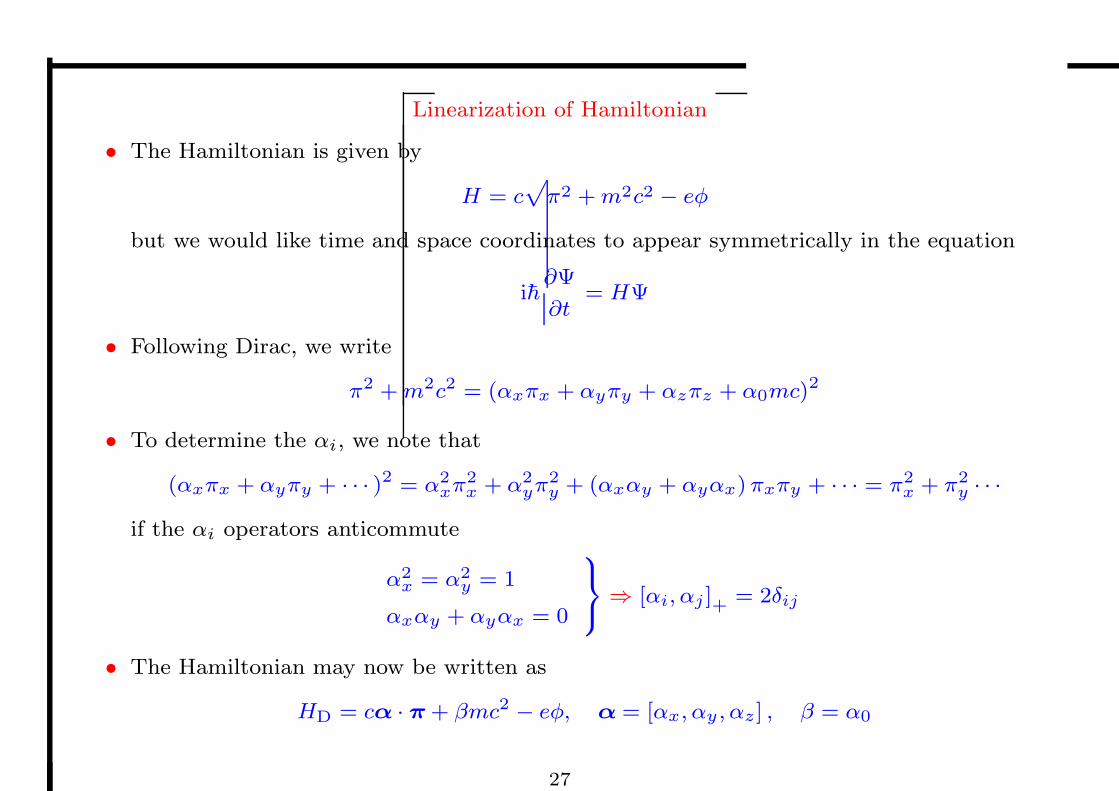
Linearization of Hamiltonian
• The Hamiltonian is given by
H = cp
π2 + m2c2 − eφ
but we would like time and space coordinates to appear symmetrically in the equation