Monetary Easing and Financial Instability∗

Viral AcharyaNew York University

Guillaume PlantinSciences Po

October 28, 2016

Abstract

We build a model to study optimal monetary policy in the presenceof financial stability concerns. Rigid output prices preclude optimalreal investment in response to preference (or productivity) shocks.Monetary easing, by lowering the cost of capital for firms, can restoreoutput to the efficient level, but also subsidizes inefficient maturitytransformation by financial intermediaries - “carry trades” that bor-row cheap at the short-term against illiquid long-term assets. Carrytrades not only lead to financial instability in the form of rollover riskfrom short-term debt, but also crowd out real investment since in-termediaries equate the marginal return on lending to firms to thaton carry trades. Optimal monetary policy trades off any stimulativegains against these costs of carry trades. The model provides a frame-work to understand the puzzling phenomenon that monetary easingis associated with low real investment, even while returns to real andfinancial capital are high.

Keywords: Monetary policy, ultra-low interest rates, quantitative easing,financial stability, financial fragility, shadow banking, maturity transforma-tion, carry trades

JEL: E52, E58, G01, G21, G23, G28

∗We are grateful to seminar and workshop participants at the World EconometricSociety Meetings, Montreal, August 2015; CREDIT Greta conference, Venice, October2015; Micro Foundations of Macro Finance workshop, New York University, April 2016;London Business School, June 2016; and, University of Mannheim, June 2016, for helpfulcomments and discussions. Hae Kang Lee provided excellent research assistance.

1

“In the absence of economic rents, the return on corporate capital should

generally follow the path of interest rates, which reflect the prevailing return

to capital in the economy. But over the past three decades, the return to

productive capital generally has risen, despite the large decline in yields on

government bonds.” – Jason Furman, Chairman of the Council of Economic

Advisors, United States, in “Productivity, Inequality and Economic Rents,”

June 13, 2016.

Introduction

Motivation

Since the global financial crisis of 2007-08, central banks in the Western

economies have embarked upon the so-called unconventional monetary poli-

cies. These policies feature monetary easing aimed at keeping interest rates

at ultra-low levels. Most notably, the Federal Reserve has kept interest rates

at the zero lower-bound with large-scale asset purchases of Treasuries and

mortgage-backed securities. European Central Bank has now followed suit

with such purchases and so has the Bank of Japan. The objective of such

aggressive easing has been to restore some of the abrupt and massive loss

in aggregate demand that followed the crisis by lowering the cost of capital

for the real sector with the objective of stimulating investment and credit to

“normal” levels.

Several academics and policy-makers have highlighted, however, that such

monetary policies have had unintended consequences that have limited the

2

effectiveness of the policies in achieving the intended goals. In particular,

they have highlighted the “search for yield” among institutional investors

and the resulting asset-price inflation in certain risky assets such as high-

yield corporate bonds and emerging-market debt and equities.1 Others, no-

tably Furman (2015, 2016) (see the introductory quote), have argued that

coincident with low rates has been a high marginal return to capital, low

fixed real investment, and high returns to shareholder capital in the form of

share buy-backs. Indeed, if extended periods of low rates were successful at

restoring investment, the marginal return of capital would end up low and

fixed real investment high. Furman considers this an important puzzle facing

economic theory and the practice of monetary policy.

One way of understanding these consequences in a unified way is that

keeping interest rates low allows financial institutions to fund long-term as-

sets with relatively short-term claims, hoping that these claims can be refi-

nanced until the long-term assets mature, resulting in a “carry.” A potential

rollover risk arises with such carry trades when the availability of future

funding liquidity is uncertain, and early liquidation of the long-term assets

backing the trades is costly and inefficient. In this case, the maturity trans-

1See, in particular, Rajan (2013): “If effective, the combination of the “low for long”policy for short term policy rates coupled with quantitative easing tends to depress yields.. . . Fixed income investors with minimum nominal return needs then migrate to riskierinstruments such as junk bonds, emerging market bonds, or commodity ETFs. . . . [T]hisreach for yield is precisely one of the intended consequences of unconventional monetarypolicy. The hope is that as the price of risk is reduced, corporations faced with a lowercost of capital will have greater incentive to make real investments, thereby creating jobsand enhancing growth. . . . There are two ways these calculations can go wrong. First,financial risk taking may stay just that, without translating into real investment. Forinstance, the price of junk debt or homes may be bid up unduly, increasing the risk ofa crash, without new capital goods being bought or homes being built. . . . Second, andprobably a lesser worry, accommodative policies may reduce the cost of capital for firmsso much that they prefer labor-saving capital investment to hiring labor.”

3

formation that monetary easing induces in the financial sector creates private

gains in the sector – resulting from transfers from savers to borrowers – but

also results in expected social costs in the form of inefficient liquidations of

long-term assets when this rollover risk materializes.

For instance, when the “taper” of its expansionary monetary policy was

announced by the Federal Reserve in May 2013, several emerging market

debt securities experienced liquidations by foreign institutional investors,

causing severe price volatility in their debt markets as well as in the cur-

rency exchange rates.2 The “taper tantrum” required massive interventions

by emerging market central banks and was ultimately calmed down only

when the Federal Reserve indicated a few months later that it would not in

fact taper as quickly as it might have suggested in May 2013. Recently, as

the Federal Reserve appears to be moving closer to “up-lift” of the rates,

similar liquidation concerns have been raised about. In particular, there is

the mention of “illusory liquidity” that the financial sector has been relying

on for funding of positions in high-yield corporate debt, structured products,

and emerging market debt and equities, and that this liquidity may vanish

with the up-lift.

Importantly, as returns to carry trades become positive when interest

rates are low, financial intermediaries allocate economy’s savings away from

real investment into paying out of carry until the marginal return on invest-

ment rises to compensate for the opportunity cost of giving up the carry. In

other words, low interest rates induce carry trades that crowd out real-sector

2See Feroli et al.(2014), who document that Emerging Market Bond Funds had startedreceiving steady inflows since 2009, with a peak of around $3.5 bln per month thatpromptly reversed to outflows of similar magnitude in the months immediately after the“taper” announcement. See also the discussion of Feroli et al. by Stein (2014).

4

investment. This leads to the coincidence of low rates with high marginal

return on real capital, low real investment, and high shareholder return on

capital (due to paying out of the carry), as documented in Furman (2015,

2016).

Model

We capture these rich economic insights in a simple and tractable framework

that can provide a building block for a fuller model of monetary policy that

faces a “penalty” when interest rates are too low. In particular, we present

a model that integrates the stimulative rationale of monetary easing with

the financial instability risk and crowding-out of real investment that arise

from carry trades induced in the financial sector by monetary easing. Our

main result is that when the stimulative gains from monetary policy are weak

and the potential for financial carry trades large, optimal monetary policy

should “lean against the wind” by tightening and discouraging carry trades.3

Interestingly, and equally importantly, the discouraging of carry trades by

keeping interest rates not too low is essential to raising aggregate demand as

this reduces the crowding-out effect.

The key ingredients of our model are as follows. We study an economy

in which the relative price of output is fixed (“nominal rigidity”), and thus

cannot reflect shocks to consumer preferences (alternatively, shocks to pro-

3While our motivation focused on the more recent monetary easing, the finan-cial instability risk we highlight has manifested also in the past episodes of mone-tary easing in the form of destabilization of long-term government bond markets (seehttp://fortune.com/2013/02/03/the-great-bond-massacre-fortune-1994/) and the materi-alization of rollover risk in mortgage-related maturity transformation by the financialsector.

5

duction costs). Corporations issue bonds and so does the public sector, all at

the going rate of interest which the central bank (assumed to be managing

debt for the public sector) can set through sale or repurchase of public sector

bonds through open market operations. Any such central bank actions in

bond markets are immediately met with tax increase or rebate. To start

with, we consider a benchmark model without the financial intermediaries.

In the case of temporary positive preference shocks for the real sector’s

output, monetary easing – by temporarily lowering the interest rate – reduces

the corporate cost of capital and can restore the first-best allocation that is

out of reach under laissez-faire because of missing price signals for the real

sector output. Effectively, as the nominal price is rigid, the central bank by

setting the nominal rate is able to set the real rate of interest to the desired

level or the natural rate.

We then introduce financial intermediaries. We assume that financial in-

termediaries can issue short-term debt to savers at the going rate of interest

and intermediaries choose how much to lend to the corporations (assumed

to be short-term) versus lending against long-term assets held by long-term

investors (capturing some or all of these assets’ returns in the process, or

equivalently, intermediaries have legacy long-term assets of their own). Fund-

ing of long-term assets by issuing short-term debt gives rise to rollover risk

if long-term assets’ cash flows are delayed and intermediaries face a freeze in

the short-term funding markets; in such case, long-term assets are liquidated

at a cost that is socially inefficient. If long-term assets’ cash flows are, how-

ever, realized early, then intermediaries receive a carry that compensates for

the rollover risk undertaken.

6

Maturity transformation in the form of such “carry trades” is privately

beneficial to financial institutions, but socially costly. It implements a trans-

fer from households to borrowing financial institutions at the social cost of

inefficient early liquidation of long-term assets when rollover risk material-

izes. There is, in addition, a more subtle social cost from the carry trades.

Intermediaries reduce lending to corporations until the marginal return on

corporate investment earned by intermediaries equals the carry-trade returns,

a crowding-out effect that is increasing in the attractiveness of carry-trade,

which in turn, increases the lower is the interest rate set by the central bank.

We then show that optimal monetary policy that incorporates these two

social costs of carry trades operates in the following way. In general, it does

not involve monetary easing up to the point in the benchmark model as this

induces carry trades and crowds out real-sector investment. Instead, the

optimal monetary policy sets the interest rate to a point that discourages

carry trades and prevents such crowding-out. In other words, it stops at a

point beyond which further monetary easing results in financial instability of

the financial sector and depression of real investment.

Finally, we extend the model to endogenize the rollover risk of the long-

term assets when funded with short-term debt. In particular, we assume

that the rollover risk is due to cash inlays required by long-term assets to

retain their value. The central bank can provide liquidity to meet such inlays

at its lender-of-last-resort (LOLR) rate to maintain ex-post real efficiency

from keeping these assets as ongoing instead of their being liquidated. We

then obtain an interesting tradeoff between the monetary policy rate and the

LOLR rate. Carry trades become only more attractive with a low LOLR

7

rate, so that optimal policy either features (i) a low monetary policy rate

combined with a high LOLR rate (“aggressive” policy that discourages of

carry trades at the cost of ex-post efficiency), or (ii) a high monetary policy

rate combined with a low LOLR rate (“conservative” policy that discourages

carry trades at the cost of lower ex-ante investment).

The model, in turn, also provides implications for when quantitative eas-

ing programs may be efficient and succeed without inducing financial insta-

bility. If the aggressive policy above cannot be implemented due to time-

inconsistency problem in setting the LOLR rate, then the central bank can

compensate by reducing the supply of long-term assets in the economy that

facilitate carry trades. In particular, it would not help with financial stabil-

ity to purchase assets with high rollover risk that are not attractive for carry

trades in the first place, but safer and more liquid long-term assets that lend

themselves to carry-trade profits when short-term funding costs are low.

The paper is organized as follows. Section 1 describes the related litera-

ture and our contributions relative to it. Section 2 presents the benchmark

model of monetary easing with nominal rigidity. Section 3 introduces finan-

cial intermediaries and derives (i) the carry-trade incentives for optimal rate

in the benchmark model, (ii) implications of the carry trades, and, (iii) the

optimal monetary policy taking account of carry trades by the financial sec-

tor. Section 4 extends the model to a lender-of-last-resort (LOLR) policy,

so that the central bank sets the ex-ante policy rate as well as the ex-post

LOLR rate when rollover risk materializes, and also discusses implications

for quantitative easing programs. Section 5 presents the concluding remarks.

8

1 Related literature

It is interesting to contrast the role of monetary easing in creating financial

instability in our model from the current literature that models this role.

In Farhi and Tirole (2012), the central bank faces a commitment problem

which is that it cannot commit not to lower interest rates when financial sec-

tor’s maturity transformation goes awry. In anticipation, the financial sector

finds it optimal to engage in maturity transformation to exploit the central

bank’s “put.” In contrast, in our model the central bank faces no commit-

ment problem as such, but it finds low rates attractive from the standpoint

of stimulating productive investment and must weigh this benefit against the

cost that low rates also stimulate inefficient maturity transformation in the

financial sector.

In Diamond and Rajan (2012), the rollover risk in short-term claims dis-

ciplines banks from excessive maturity transformation, but the inability of

the central bank to commit to “bailing out” short-term claims removes the

market discipline, inducing excessive illiquidity-seeking by banks. They too

propose raising rates in good times taking account of financial stability con-

cerns, but so as to avoid distortions from having to raise rates when banks

are distressed. Again, the contrast with our model is that central bank in

our model has no commitment problem but its attempts to boost activity by

lowering rates induce carry trades.

Acharya and Naqvi (2012a) develops a model of internal agency problem

in financial firms due to limited liability wherein liquidity shortfalls on matu-

rity transformation serve to align insiders’ incentives with those of outsiders.

When aggregate liquidity at rollover date is abundant, such alignment is

9

restricted accentuating agency conflicts, leading to excessive lending and fu-

eling of asset-price bubbles. Acharya and Naqvi (2012b) argue that monetary

policy being easy only exacerbates this problem and that it should instead

lean against the wind to get around the limited-liability induced distortions

in bank lending. Our model features, in contrast, carry trade behavior that

is entirely due to moral hazard created by the monetary policy, even absent

agency problems within the financial sector.

Stein (2012) explains that while prudential regulation of banks and sys-

temically important financial firms can partly rein in the attempts to engage

in excessive maturity transformation, there is always some unchecked growth

of such activity in shadow banking. He argues for a monetary policy that

leans against the wind as raising the cost of borrowing which reaches all

“cracks” of the financial sector. Finally, Acharya (2015) proposes a leaning-

against-the-wind interest-rate policy in good times for a central bank to re-

duce the extent of political interference that can arise in attempting to deal

with quasi-fiscal actions during a financial crisis. These explanations are both

consistent with the considerations for financial stability in our model, but our

objective is to deliver a stylized model that can serve as a building block for

a fuller model of monetary policy that accounts for such considerations.

2 An elementary model of monetary easing

2.1 Setup

Time is discrete. There are two classes of agents: households and the public

sector. Households are of two types, savers and entrepreneurs, that share

10

similar preferences but differ along their endowments. There are two goods

that households find desirable: a numeraire good and entrepreneurs’ output.

Households’ preferences. At each date, a mass 2 of households are

born and live for two dates. Each cohort is equally split into savers and en-

trepreneurs. Both types of households derive utility from consumption only

when old. Entrepreneurs’ output and the numeraire good are perfect substi-

tutes for them, although an entrepreneur cannot consume his own output.

Households are risk neutral over consumption.

Households’ endowments. Each saver receives an endowment of y

units of the numeraire good at birth, where y > 0. Each entrepreneur born

at date t is endowed with a technology that transforms an investment of I

units of the numeraire good at date t into f(I) units of output at date t+ 1.

The function f satisfies the Inada conditions and is such that

f ′(y) < 1. (1)

Public sector. The public sector does not consume and maximizes total

households’ utility, discounting that of future generations with a factor arbi-

trarily close to 1. At each date, the public sector matches net bond issuances

described below with lump sum rebates/taxes to current old households.

Bond markets. There are two markets for one-period risk-free bonds

denominated in the numeraire good. The public sector and savers trade in

the public-bond market. Savers and entrepreneurs trade in the corporate-

bond market. Note that this implies in particular that the public sector

cannot lend to entrepreneurs.4

4Note also that restricting corporate securities to risk-free bonds is only to fix ideas.

11

Monetary policy. The public sector announces at each date an interest

rate at which it is willing to meet any (net) demand for public bonds by

savers.

Finally, households are price-takers in goods and bonds markets.

Comments

This setup is a much simplified version of the workhorse monetary model

in which money serves only as a unit of account (“cashless economy”) and

monetary policy boils down to enforcing a short-term nominal interest rate.

In the workhorse model, the presence of nominal rigidities implies that the

monetary policy also affects the real interest rate. Below, we dramatically

simplify this workhorse framework by assuming extreme nominal rigidities

in the form of a fixed price level for one good that we therefore deem the

numeraire good. Beyond obvious gains in tractability, our motivation for this

simplification is that it is useful to study how financial-stability concerns

stand in the way of a central bank in a benchmark model in which the

monetary authority would otherwise have a free hand at controlling the real

economy.

2.2 Steady-state

We study steady-states in which the public sector announces a constant in-

terest rate r > f ′(y), and the price of firms’ output (in terms of the numeraire

good) is at its equilibrium level of one.

This comes at no loss of generality given that production is deterministic and entrepreneursface no financial frictions.

12

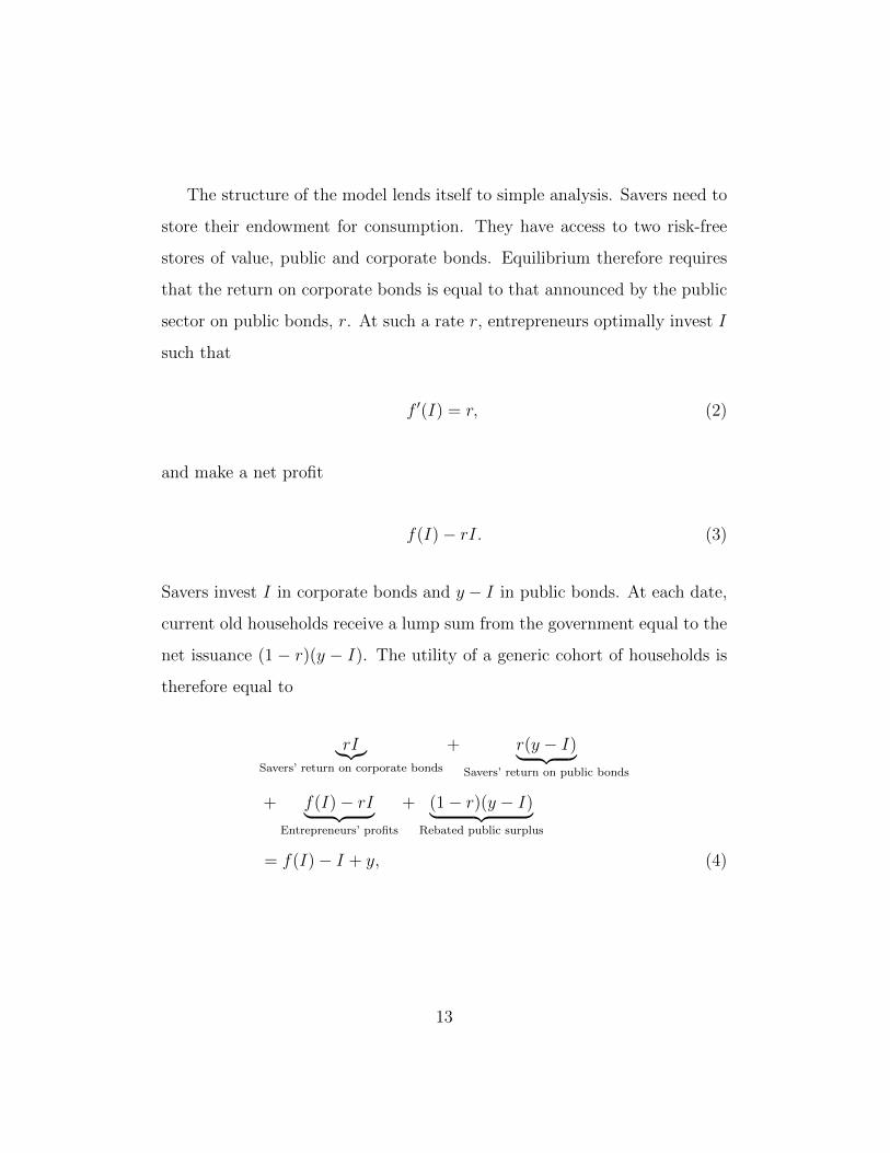
The structure of the model lends itself to simple analysis. Savers need to

store their endowment for consumption. They have access to two risk-free

stores of value, public and corporate bonds. Equilibrium therefore requires

that the return on corporate bonds is equal to that announced by the public

sector on public bonds, r. At such a rate r, entrepreneurs optimally invest I

such that

f ′(I) = r, (2)

and make a net profit

f(I)− rI. (3)

Savers invest I in corporate bonds and y − I in public bonds. At each date,

current old households receive a lump sum from the government equal to the

net issuance (1 − r)(y − I). The utility of a generic cohort of households is

therefore equal to

rI︸︷︷︸Savers’ return on corporate bonds

+ r(y − I)︸ ︷︷ ︸Savers’ return on public bonds

+ f(I)− rI︸ ︷︷ ︸Entrepreneurs’ profits

+ (1− r)(y − I)︸ ︷︷ ︸Rebated public surplus

= f(I)− I + y, (4)

13

maximized at

f ′(I∗) = r∗ = 1. (5)

In this elementary environment, condition (5) rephrases the standard “golden

rule” according to which steady-state consumption is maximum when the

return on savings equates the growth rate of the economy (zero here). Net

public debt issuance is zero at each date at this optimal unit interest rate.

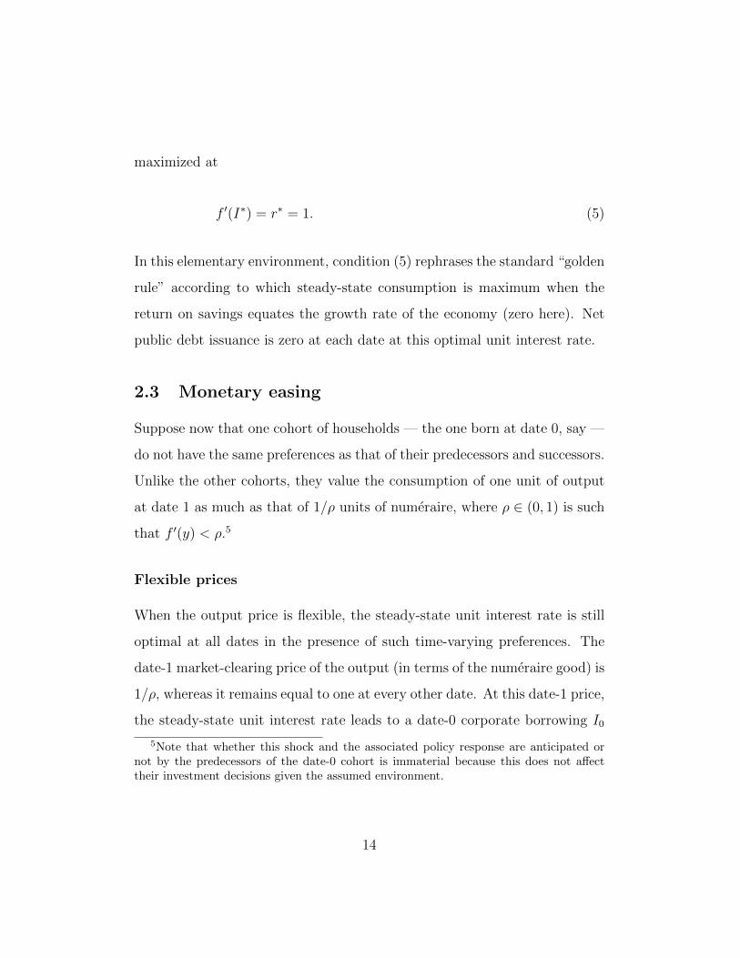
2.3 Monetary easing

Suppose now that one cohort of households — the one born at date 0, say —

do not have the same preferences as that of their predecessors and successors.

Unlike the other cohorts, they value the consumption of one unit of output

at date 1 as much as that of 1/ρ units of numeraire, where ρ ∈ (0, 1) is such

that f ′(y) < ρ.5

Flexible prices

When the output price is flexible, the steady-state unit interest rate is still

optimal at all dates in the presence of such time-varying preferences. The

date-1 market-clearing price of the output (in terms of the numeraire good) is

1/ρ, whereas it remains equal to one at every other date. At this date-1 price,

the steady-state unit interest rate leads to a date-0 corporate borrowing I0

5Note that whether this shock and the associated policy response are anticipated ornot by the predecessors of the date-0 cohort is immaterial because this does not affecttheir investment decisions given the assumed environment.

14

such that

f ′(I0)

ρ= 1, (6)

that exceeds the level I∗ prevailing at other dates. The objective of the public

sector is reached at this unit rate because production is efficient at each date.

Redistributive implications of the preference shock

The exceptionally high date-0 productive investment level I0 > I∗ has redis-

tributive consequences across cohorts that are immaterial given the public

sector’s objective. At date 0, the public sector faces a bond payment of

y− I∗ to the date-(−1) cohort but raises only y− I0 from the date-0 cohort.

It therefore must collect a lump sum tax I0 − I∗ from old date-(−1) house-

holds.6 At date 1, the public sector repays only ρ(y−I0) to the date-0 cohort

whereas it collects y − I∗ from the date-1 cohort. Overall, the utility of the

date-0 cohort is:

f(I0)

ρ− ρI0

︸ ︷︷ ︸Entrepreneurs’ profits

+ ρ(y − I0)︸ ︷︷ ︸Public bonds return

+ ρI0︸︷︷︸Private bonds return

+ y − I∗ − ρ(y − I0)︸ ︷︷ ︸Date-1 public rebate

=f(I0)

ρ− I0 + y

︸ ︷︷ ︸Surplus created by the date-0 cohort

+ I0 − I∗︸ ︷︷ ︸Subsidy from other cohorts

. (7)

The subsidy from other cohorts I0 − I∗ matches the tax paid by the

date-(−1) cohort at date 0.

6Recall our convention that households are taxed when old only.

15

Nominal rigidities and optimal monetary policy

We now create room for active monetary policy at date 0 by introducing

nominal rigidities:

Assumption. (Sluggish output price) The output price remains constant

at all dates at its steady-state level of one.

In other words, we suppose that the price system is too rigid to track

the exceptional and transitory preference shock that hits the date-0 cohort.7

With sticky output price, the public sector can make up for the absence of

appropriate price signals in the date-1 output market by distorting the date-0

capital market. Monetary easing in the form of an interest rate equal to ρ

between dates 0 and 1 boosts date-0 productive investment to the optimal

level I0 because optimal date-0 investment by entrepreneurs then derives

from the very same equation (6). The only difference with the case of flexible

prices is that date-0 entrepreneurs’ profit is reduced to f(I0) − ρI0 because

the consumers of their output extract a surplus (1/ρ)f(I0)− f(I0) given the

unit output price.

Proposition 1. (Monetary easing) Setting the interest rate at ρ at date

0 and at one at other dates implements the flexible-price outputs and is there-

fore optimal.

Proof. See discussion above. �

This very stylized model of monetary easing shares with the New-Keynesian

framework the broad view that monetary policy serves to mitigate welfare

7We could also assume a partial price adjustment without affecting the analysis.

16

losses due to the relative price distortions induced by nominal rigidities (see,

e.g., chapter 4 in Galı, 2015). In our setup, however, the important price dis-

tortion occurs between sectors of varying interest-rate sensitivities. We nat-

urally interpret the entrepreneurs as representing the most interest-sensitive

(non-financial) sectors of the economy, such as construction and other durable

goods manufacturers. Accordingly, the date-0 preference shock captures in

a fixed-price environment the idea that durables would be relatively more

affected in a deflationary environment, as seems to be empirically the case.8

3 Monetary policy and financial instability

We now introduce a financial sector in this economy. The financial sector is

comprised of two types of agents, banks and long-term investors. Both banks

and LT investors find only the numeraire good desirable. They are risk-

neutral over consumption at each date. They discount future consumption

using the same discount factor as that of the public sector. (Recall this

discount factor is arbitrarily close to 1). Banks and LT investors play the

following respective roles in the economy.

Banks. We shut down the corporate-bond market and suppose instead

that the financing of entrepreneurs by savers must be intermediated by

banks. To fix ideas, we suppose that savers are competitive in the mar-

ket for deposits—one-period risk-free bonds issued by banks, and that banks

are competitive in the market for loans—one-period risk-free bonds issued

8See Klenow and Malin (2011) for the empirical link between durability and price flex-ibility. In fact, we could equivalently assume time-invariant preferences and an exogenousdate-0 drop in the output price.

17

by entrepreneurs. Savers still have direct access to government bonds. Fol-

lowing Diamond (1997), we model liquidity risk for banks as a simple form

of market incompleteness. We suppose that each bank has access to capital

markets with probability 1− q only at each date, where q ∈ (0, 1). Penalties

from defaulting on deposits are so large that banks never find it optimal to

do so.

LT investors. At date 0, LT investors hold claims to an asset that pays

off A at a random future date with arrival probability p ∈ (0, 1).9 All or part

of the asset can also be liquidated before this accrual date at a linear cost: It

is possible to generate cash at the current date at the cost of giving up 1 +λ

units at the accrual date for each currently generated unit, where λ ≥ 0. LT

investors cannot trade directly with households but can do so with banks.

Finally, we suppose that exclusions from markets are not perfectly cor-

related across banks, and that the exclusion dates are independent from the

asset’s payoff date.

The model studied in Section 2 can be viewed as the particular case in

which A = 0 so that LT investors are immaterial. In this case, banks cannot

remunerate deposits below the return on public bonds and entrepreneurs can-

not borrow below the deposit rate. Banks’ assets and liabilities therefore all

earn the policy rate at all dates, banks make zero profit and are immaterial.

9This specification of a payoff date arriving at a constant rate is meant to obtaina simple time-homogeneous problem. All that matters is that the asset is long term(p < 1). We could also introduce heterogeneous assets of varying maturities withoutgaining significant insights.

18

3.1 Inefficient carry trades

The financial sector becomes relevant when A > 0. We focus on the most

interesting case in which

A ≥ y. (8)

In this case, monetary easing at date 0 in the form of a policy rate equal

to ρ between dates 0 and 1 opens up potential gains from trade between

banks and LT investors. Banks have access to funds at a lower cost than

the financial sector’s discount factor, and LT investors own claims to future

consumption against which it is possible to borrow. Thus banks can enter

into profitable carry trades by buying assets from LT investors, financing

their acquisitions by rolling over short-term debt until the accrual date at

which the trade is unwound. To fix ideas, we suppose that banks extract all

the gains from such trades with LT investors. Our results rely only on the fact

that they extract at least some of these gains. Note that this assumption that

LT assets trade in a buyer’s market is consistent with condition (8) which

states that there is little money chasing many assets.

Such carry trades involve risky maturity transformation. If a bank is

excluded from markets before the asset pays off, then it must liquidate its

LT assets in order to honor outstanding deposits. This illiquidity risk reduces

the appeal of carry trades.10

Formally, suppose that a bank finances the purchase of a claim to a unit

10For simplicity, we suppose that banks have a sufficient initial endowment in assetsidentical to the ones they purchased from LT investors that they can always generateenough cash from early liquidation when cut from markets.

19

payoff from LT investors with the issuance of a unit deposit at date 0. The

expected value of the associated liability is then:

ρ∑

k≥1

(1− q)k−1(1− p)k−1[p+ (1− p)q(1 + λ)] = ρ(1 + Λ), (9)

where

Λ =λ

1 + p(1−p)q

. (10)

Expression (9) states that the bank rolls over the unit deposit until the first

of two events occurs: the accrual date or an exclusion date. The latter event

entails early liquidation of LT assets.

The parameter Λ defined in (10) is increasing in λ, 1− p, and q. It thus

measures the overall magnitude of the transformation risk induced by carry

trades.

If ρ(1 + Λ) ≥ 1, then the carry trade is not profitable. LT investors hold

on to their assets, and banks intermediate between savers and entrepreneurs

the optimal investment I0 at date 0 making zero profit.

Conversely, if ρ(1+Λ) < 1, then banks have two valuable alternative uses

of deposits. They may either lend to entrepreneurs, or engage in carry trades.

The marginal return on carry trades is one minus the expected cost of failure

to roll over ρΛ. In equilibrium, the marginal return on loans to entrepreneurs

must equate it. This implies that banks attract the entire date-0 savers’ in-

come y and split their investments into an aggregate lending to entrepreneurs

I∗∗ and a carry trade of size y− I∗∗, where I∗∗ is the entrepreneurs’ demand

20

for funds when the cost of funds is 1− ρΛ:

f ′(I∗∗) = 1− ρΛ. (11)

Note that banks, unless excluded from markets, have enough funds to both

lend I∗ to entrepreneurs and refinance the carry trade y − I∗∗ at all t ≥ 1.11

The following proposition summarizes these results.

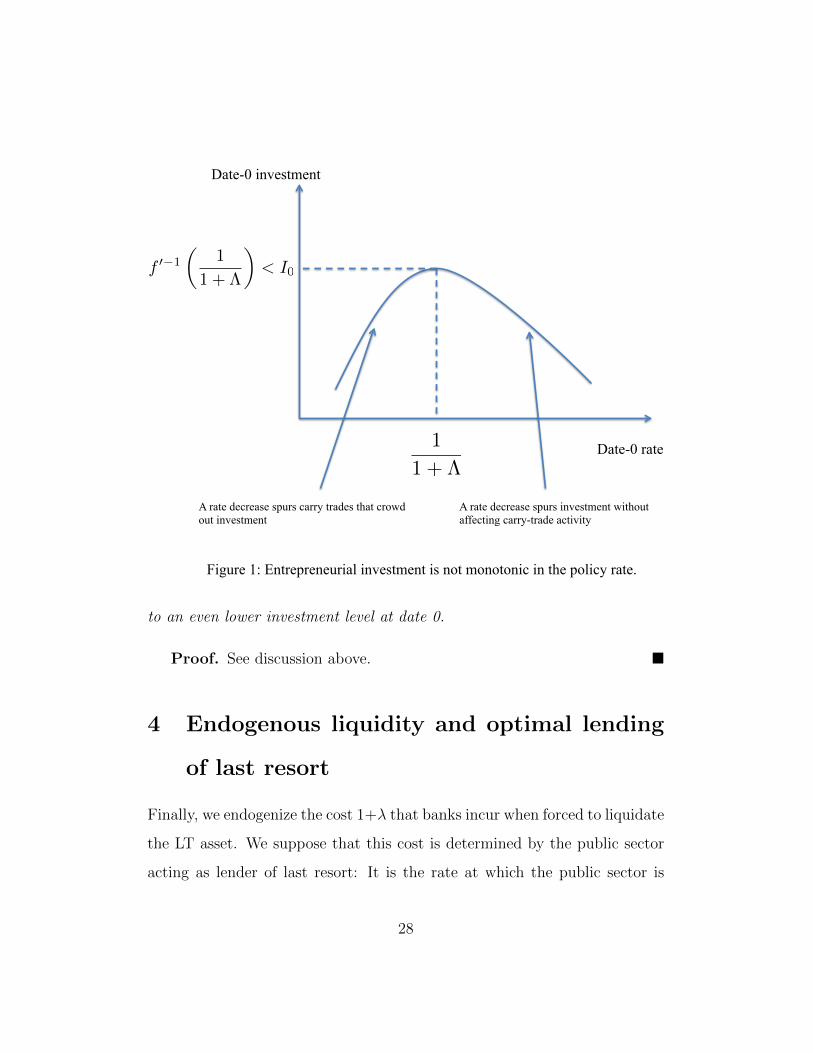
Proposition 2. (Monetary easing and inefficient carry trades) If

ρ(1+Λ) ≥ 1, then banks do not enter into carry trades at date 0. They make

zero profit and channel I0 towards entrepreneurs at date 0.

Otherwise, entrepreneurs invest only I∗∗ such that I∗ < I∗∗ < I0. Banks

use the residual date-0 savings y − I∗∗ to enter into carry trades at date 0,

where f ′(I∗∗) = 1 − ρΛ. In particular, the public sector has no resources at

date 0.

Proof. See discussion above. �

This setup captures the idea that imposing an unusually low interest rate

creates room for socially inefficient carry trades. Carry trades are socially

inefficient for two reasons: they create financial instability and they crowd

out productive investment.

• Financial instability. The return on carry trade 1 − ρ(1 + Λ) can be

decomposed in two parts, a “carry” 1 − ρ and an expected cost of fi-

nancial distress −ρΛ. The carry is a wash for social surplus as it is

only a transfer from households to banks via the diversion of govern-

11This stems from ρ(y − I∗∗) < y − I∗ since I∗∗ > I∗.

21

ment surplus.12 On the other hand, the expected cost of the liquidity

crises created down the road by maturity transformation is a social

deadweight loss. In other words, banks extract rents at the social cost

of financial instability.

• Crowding out of productive investment. The additional social cost of

carry trades is that carry-trade returns raise the hurdle rate for loans to

entrepreneurs, thereby leading to a suboptimally low level of produc-

tive investment. Note that this second source of inefficiency prevails

only if the wealth to income ratio A/y of the economy is sufficiently

large, as is the case under condition (8), so that the marginal deposit

has two alternative uses in equilibrium, either carry trades or loans to

entrepreneurs. A sufficiently small supply of assets against which banks

find it profitable to rollover deposits would imply that the hurdle rate

on loans would be ρ.

3.2 Model Interpretation and Implications

Interpretation of A ≥ y

We interpret condition (8) as essentially stating that maturity/liquidity trans-

formation by the banking system—short-term borrowing against long-term

cash assets—is not constrained by prudential regulation. The public sector

could in principle control carry-trade activity by banks by means of appro-

priate prudential rules. Assuming away such a binding regulation in the

United States is in line with the existence of a shadow banking system prior

12Absent carry trades, the government rebates the carry 1−ρ to current old households.

22

to 2007 that was larger than the traditional banking system, and that was

not subject to such rules. In line with our theory, the shadow banking sys-

tem in the presence of stricter macro-prudential regulation since 2007 has

sharply contracted, but the carry trades appear to have moved over to as-

set management industry flows into junk bonds and collateralized leveraged

loans (Stein, 2014), and emerging market government and corporate bonds

(Feroli et al. 2014). IMF GFSR (2016) documents that the presence of such a

“risk-taking channel” in the non-bank finance (insurance companies, pension

funds, and asset managers) to low rates implies that monetary policy remains

potent in affecting economic outcomes – we argue, in potentially unintended

and harmful ways – even when banks face strict macroeconomic regulation.

Crowding out by “carry trades”: Empirical evidence

Our setup predicts several of the stylized facts described in the introduction

(Furman, 2015, 2016):

(1) Suppose that p is large and q small, other things being equal, i.e., the

long-term assets are relatively safe and face low rollover risk. Then 1 − ρΛ

is large and crowding out is important: There is limited real investment

by entrepreneurs and the marginal return to real sector capital is high in

equilibrium.

(2) It is likely that the refinanced asset pays off before a liquidity crisis

(in which many banks become excluded from trading and get distressed).

At this payoff date, the carry accrues to banks: The return on shareholder

capital is high due to high payouts but carries the rollover risk.13

13An alternative interpretation of this payout is in the form of issuance of bonds by

23

Note that if banks and LT investors were splitting the surplus from carry

trades, then payouts by banks would be smaller but there would be an initial

boom in asset prices from LT assets at date 0. Alternatively, the LT assets

can be interpreted as foreign assets chased by international capital flows

searching for yield (Feroli et al. 2014).

Malinvestment

The mechanism that leads inefficient carry trades to arise and crowd out

investment closely relates to the old notion of “malinvestment that is promi-

nent in Austrian economics (Hayek, 1931, and von Mises, 1949, for example).

The distortion of the real interest rate due to monetary easing may subsi-

dize activities that are not socially desirable, e.g., excessive lending to the

housing sector, but become privately profitable for banks due to the (socially

inefficient) maturity transformation they offer, at the expense of more desir-

able investments such as loans to the real sector. Whereas rent extraction

through inefficient maturity transformation or carry trades are a particularly

relevant and topical form of “malinvestment,” this distortion can and does

take other forms such as zombie lending by banks which we discuss next.

Zombie lending

Inefficient speculation is not the only unintended consequence of monetary

easing that observers have pointed out in recent crises. In some contexts,

corporations to engage in shareholder buy-backs without undertaking significant real in-vestment. In other words, corporations can themselves engage in “carry trades” by tappinginto bond markets, a financial “arbitrage” of sorts that creates value for shareholders onits own.

24

such as Japan in the 1990s following monetary easing by the Bank of Japan

(Caballero, Hoshi and Kashyap, 2008, and Gianetti and Simonov, 2013), or

Italy and Spain after European Central Bank’s unconventional monetary pol-

icy actions in 2012 (Acharya, Eisert, Eufinger and Hirsch, 2015), the main

concern has rather been that of zombie lending—the refinancing of highly

distressed borrowers in order to defer credit losses at the risk of amplifying

them down the road. It is straightforward to introduce this unintended con-

sequence of monetary easing in our setup. Suppose for example that banks

have legacy non-performing loans that can be either liquidated at date 0 or

refinanced for one additional period, which creates an additional loss δ at

date 1 for each dollar of refinancing. In other words, zombie lending is a

storage technology with return 1 − δ. Investing deposits in this technology

becomes appealing if the date-0 policy rate is lower than 1− δ. This creates

deadweight losses and crowding out of productive investment very much in

the same way as in the case of maturity transformation or carry trades.

Redistributive implications of carry trades

Recall that, absent carry trades (ρ(1 + Λ) ≥ 1), monetary easing entails that

the date-0 cohort receives a subsidy I0 − I∗ that is paid by the date-(−1)

cohort when old at date 0. In the presence of carry trades, the date-(−1)

cohort pays a larger tax y−I∗ to the public sector at date 0 because all fresh

resources y are directed towards banks at this date. The public sector must

essentially default on this cohort, which in this setting takes the form of a

lump sum tax equal to the repayment owed. The counterpart of this tax is

an equivalent public surplus paid to the date-0 cohort at date 1 since the

25

government receives funds from young households and owes nothing to old

households at this date 1. In addition, banks extract (at the cost of liquidity

risk) a carry (1 − ρ)(y − I∗∗). In sum, carry trades increase the loss to old

households at date 0 at the benefit of banks.14

Interbank market

The assumption that banks lose all access to funds when excluded from the

market simplifies the analysis but is rather strong. We could alternatively

assume that banks may randomly lose direct access to retail deposits, but

that they could still gain indirect access to funding via other banks in an

interbank market, albeit at some cost. This way, banks would be able to

insure each other against liquidity risk. Because this risk is the only force that

reduces their incentives to enter into carry trades, the crowding-out effect of

carry trades would be even stronger under this milder assumption. More

generally, since intermediaries internalize the rollover risk of carry trades

in our models, long-term assets with greater safety and liquidity such as

government bonds, collateralized assets, and other fixed-income securities,

become more attractive havens for carry trades, and the more liquid these

assets are, the greater is the ex-ante crowding out of real investment.

3.3 Optimal monetary policy

Section 3.1 studied the situation in which the public sector naively sets the

date-0 policy rate at the level ρ that is optimal absent opportunistic behavior

14These redistributive effects do crucially hinge on the assumption that only old house-holds are taxed.

26

by the financial sector. We now characterize the optimal date-0 policy rate

in the presence of such behavior. It is obviously equal to ρ when carry trades

are not profitable because ρ(1 + Λ) ≥ 1.

Consider now the interesting case in which ρ(1 + Λ) < 1. The date-0

investment in the productive technology I is not monotonic in the date-0

interest rate r set by the public sector (see Figure 1 for an illustration). For

r ∈ (1/(1 + Λ),+∞), the private sector does not enter into carry trades and

I is a decreasing function of r given by

f ′(I) = r. (12)

Otherwise, there is carry-trade activity and I is an increasing function of

r implicitly defined by

f ′(I) = 1− rΛ, (13)

because a higher interest rate makes carry trades less attractive relative to

productive investment. Thus the optimal rate set by the public sector is

1/(1 + Λ) > ρ, because it yields the highest possible level of investment in

the productive technology, which is still lower than the first-best level. To

sum up,

Proposition 3. (Optimal interest rate) If ρ(1+Λ) ≥ 1, then the optimal

policy rate is ρ which implements the first-best date-0 investment level.

Otherwise, the optimal policy rate is 1/(1+Λ), leading to a smaller second-

best level of date-0 productive investment. At a rate lower than this optimal

rate, socially inefficient carry trades crowd out productive investment leading

27

Date-0 rate

Date-0 investment

A rate decrease spurs investment without affecting carry-trade activity

A rate decrease spurs carry trades that crowd out investment

Figure 1: Entrepreneurial investment is not monotonic in the policy rate.

1

1 + ⇤

f 0�1

✓1

1 + ⇤

◆< I0

to an even lower investment level at date 0.

Proof. See discussion above. �

4 Endogenous liquidity and optimal lending

of last resort

Finally, we endogenize the cost 1+λ that banks incur when forced to liquidate

the LT asset. We suppose that this cost is determined by the public sector

acting as lender of last resort: It is the rate at which the public sector is

28

willing to lend against these LT assets.

Formally, the public sector now sets two interest rates. The first one, the

only rate that we considered thus far, is the interest rate at which claims

to future public surpluses trade at date 0. We deem it the “policy” rate,

now denoted rP .15 The second one is the rate at which the public sector

is willing to lend against LT assets, and we deem it the “lending-of-last-

resort (LOLR)” rate, denoted rL. These two rates are a stylized summary of

monetary policies that consist in controlling both short-term nominal rates

and the conditions under which each asset class is admissible collateral for

the central bank.

Absent any commitment problem nor any other ingredient in the model,

the public sector would easily implement the first-best by committing to

rP = ρ, and to a sufficiently high LOLR rate rL that discourages carry trades

in the first place.16 Since banks use public refinancing only for the socially

bad reason that they have entered into carry trades, such a high LOLR rate

would come at no cost in equilibrium. We now consider a more interesting

situation in which banks also have socially good reasons to resort to public

refinancing, so that the public sector faces a trade-off when determining the

liquidity of LT assets through its LOLR policy.

4.1 Optimal lending of last resort

We now suppose that, from date 1 on, banks may receive a profitable oppor-

tunity to lend against LT assets. The arrival rate of this opportunity is σ

15The policy rate is optimally set to 1 at all dates other than 0.16The LOLR rate must satisfy ρ[1 + (rL − 1)/(1 + pq/1− p)] ≥ 1.

29

(strictly) before the LT asset pays off, and 0 afterwards. This opportunity

requires an investment l and generates a payoff l+d at the date at which the

LT asset pays off. There are several possible interpretations for this oppor-

tunity. First, it may be construed as the financing of a subset of LT investors

against some of their assets if these agents have a preference shock and put

a premium d/l on current consumption at the arrival date. Alternatively,

it may be that a maintenance investment of l is required in order to avoid

a reduction d in the LT asset’s payoff. The public sector does not observe

whether and when this opportunity arrives and thus cannot condition its

policy on it.

For simplicity, we suppose in this section that

f(x) = log x (14)

and impose parameter restrictions:

ρ

(l + d

l

)< 1, (15)

l ≤ dy

l + d. (16)

We will explain the respective roles of these restrictions in due course.

A trade-off now arises as a higher LOLR rate rL makes a low date-0 policy

rate rP more conducive to entrepreneurial investment by discouraging carry

trades, but may eliminate such socially desirable investment opportunities.

This leads to the existence of two locally optimal policies (rP , rL):

Proposition 4. (Optimal policies) There are two locally optimal policies

30

(rP , rL). First, an aggressive policy leads to optimal date-0 investment but

comes at the cost of a strict LOLR policy that eliminates efficient subsequent

lending. Formally, it consists in setting

rP = ρ, (17)

rL > 1 +1− ρρ

[1 +

p

(1− p)q

]. (18)

The second one, more conservative, is such that

rP =l

l + d> ρ, (19)

rL = 1 +d

l

[1 +

p

(1− p)q

], (20)

which leads to a suboptimal level of entrepreneurial investment at date 0 but

maintains the socially desirable subsequent loans backed by the LT asset.

The former aggressive policy is preferable to the latter conservative one if

and only if:

log

[ρ(l + d)

l

]<ρ(l + d)

l− 1− ρσ(1− p)d

σ(1− p) + p. (21)

Proof. The banks’ subsequent lending opportunity has a private positive

NPV if and only if

l + d ≥ l

[1 +

rL − 1

1 + p(1−p)q

]. (22)

Condition (15) implies that if rL satisfies this condition, then it is not possible

to implement the investment level I0 at date 0 because setting the policy

31

rate at ρ would induce carry trades. There are therefore two local optima.

The public sector may seek to reach entrepreneurial investment I0 at date

0, in which case it must set rP = ρ and rL sufficiently large to discourage

carry trades (as given in (18)). Alternatively, the public sector may pick the

lowest rate rL at which banks invest l after date 1 whenever they have a

chance, given by (20), which imposes rP as given by (19) from Proposition

3. Condition (16) ensures that banks can raise enough funds from savers to

finance this lending opportunity l when it occurs as well as the optimal unit

loan to entrepreneurs.

Finally, (21) simply stems from noting that entrepreneurs invest 1/rP

when the date-0 policy rate is rP and from re-arranging the condition:

log(

1ρ

)

ρ− 1

ρ>

log(l+dl

)

ρ− l + d

l+

σ(1− p)dσ(1− p) + p

. (23)

�

4.2 Quantitative easing as a crowding-out strategy

The aggressive policy in Proposition 4 admits an alternative interpretation in

terms of quantitative easing. Suppose that the public sector cannot commit

to a LOLR rate other than, say, rL = 1. The public sector can then purchase

at date 0 a cash flow Q generated by the LT asset such that

Q ≥ A+ I0 − y. (24)

32

This eliminates the crowding out of entrepreneurial investment by carry

trades by ensuring that the marginal entrepreneurial loan cannot be alterna-

tively directed towards carry trades. The only remaining social cost of carry

trades stems from the expected costs of financial distress for the carry trades

that are backed by the assets left in the market. Note that if the public sector

is unable to exploit the investment opportunity l available to the financial

sector, then this public asset purchase comes at the same costs as that of a

high LOLR rate that discourages such efficient investment.

Such a large-scale asset purchase can be financed either by taxation or by

issuance of short-term debt. This latter arrangement closely matches, within

our model, the one advocated by Greenwood, Hanson and Stein (2016), who

argue that the central bank should “crowd out” the issuance of short-term

debt by the financial sector by maintaining a large balance-sheet of govern-

ment bonds funded by savers in the economy. Similarly, in our model, carry

trades by the public sector crowd out carry trades by the private sector.

This rationale for QE has the interesting implication that large-scale as-

set purchases are most efficient when they withdraw assets that would lend

themselves to carry trades from the market. In particular, QE strategies

that consist in swapping assets, in particular illiquid or long-term ones for

more liquid/shorter-lived ones, such as operations “twist” would be counter-

productive here as they would raise the profitability of carry trades and thus

lead to more crowding out of entrepreneurial investment.17

17Caballero and Farhi (2016) reach similar conclusions regarding the efficiency of assetswaps albeit for different reasons.

33

5 Concluding remarks

Our attempt in this paper has been to embed financial stability concerns in

workhorse monetary policy models. In particular, we introduced the follow-

ing tension in a monetary policy model with nominal rigidities: monetary

easing, not only lowers the cost of capital for firms, but also subsidizes inef-

ficient maturity transformation by financial intermediaries - ”carry trades”

that borrow cheap at the short-term against illiquid long-term assets. Op-

timal monetary policy trades off any stimulative gains against the costs of

carry trades from rollover risk faced by the financial sector from undertak-

ing carry trades and the crowding out of real investments. The model helps

understand the puzzle raised by Furman (2015, 2016) as to why low nominal

rates have been associated with low investment and high marginal returns

to real capital while generating at the same time high returns to shareholder

capital.

There are many directions in which we could extend our analysis fruit-

fully. One, we assumed that long-term assets are held by long-term investors

and financial intermediaries lend against these by borrowing short-term, cap-

turing in the process some or all of the long-term assets’ returns. In general,

there may be sales of some of these assets to financial intermediaries as well

as the creation of new such long-term assets. Endogenizing ex-ante asset

prices of long-term assets when carry trades are profitable is a promising di-

rection to develop a theory of asset-price inflation and bubble-burst patterns

arising as a finacial-sector response to monetary easing.

Second, we could introduce uncertainty to real-sector output or to pref-

erence shocks over time whereby monetary easing may continue for several

34

periods and then be tightened at the cost of unwinding of financial sector

carry-trades. Carry trades would then potentially build up in the economy

over an extended period of monetary easing and face abrupt rollover risk

when rates rise. Adding such a feature to the model would allow us to re-

late in a better fashion to phenomena in asset markets and financial flows as

observed during the “taper tantrum” in 2013 (Feroli et al. 2014).

Finally, our model relied on moral hazard induced by monetary easing as

a way of generating carry trades in equilibrium. Implicitly, we assumed that

the central bank cannot perfectly observe and rule out inefficient maturity

transformation or carry trades by the (shadow-banking) financial sector. It is

straightforward to consider an adverse-selection framework in which there are

two types of financial intermediaries: one, that only lend to the productive

real sector, and another, that has excess to the carry-trade technology. The

model with adverse selection has outcomes that are almost isomorphic to the

one with moral hazard: optimal monetary policy under adverse selection uses

higher interest rates or tightening to screen out the second type of financial

intermediaries by making carry trades unattractive.

References

Acharya, Viral V. 2015. “Financial Stability in the Broader Man-

date for Central Banks: A Political Economy Perspective.” Brookings’

Hutchins Center Working Paper Series.

Acharya, Viral V., Tim Eisert, Christian Eufinger, and Chris-

tian Hirsch. 2015. “Whatever it Takes: The Real Effects of Un-

35

conventional Monetary Policy.” Working Paper, NYU Stern School of

Business.

Acharya, Viral V., and Hassan Naqvi. 2012a. “The Seeds of a

Crisis: A Theory of Bank Liquidity and Risk Taking over the Business

Cycle.” Journal of Financial Economics 106 (2): 349–366.

Acharya, Viral V., and Hassan Naqvi. 2012b. “Bank Liquidity

and Bubbles: Why Central Banks Should Lean against Liquidity.” In

New Perspectives on Asset Price Bubbles: Theory, Evidence and Pol-

icy, edited by Douglas Evanoff, George Kaufman and A.G. Malliaris.

New York: Oxford University Press.

Caballero, Ricardo J. and Emmanuel Farhi. 2016. “The Safety

Trap,” Working Paper, Harvard University.

Caballero, Ricardo J., Takeo Hoshi and Anil K. Kashyap. 2008.

“Zombie Lending and Depressed Restructuring in Japan.” American

Economic Review 98 (5): 1943–77.

Diamond, Douglas W. 1997. “Liquidity, Banks, and Markets.” Jour-

nal of Political Economy 105 (5): 928–56.

Diamond, Douglas W., and Raghuram G. Rajan. 2012. “Illiq-

uid Banks, Financial Stability, and Interest Rate Policy.” Journal of

Political Economy 120 (3): 552–591.

Farhi, Emmanuel, and Jean Tirole. 2012. “Collective Moral Haz-

ard, Maturity Mismatch, and Systemic Bailouts.” American Economic

Review 102 (1): 60–93.

36

Feroli, Michael, Anil K. Kashyap, Kermit Schoenholtz, and

Hyun Song Shin. 2014. “Market Tantrums and Monetary Policy.”

U.S. Monetary Policy Forum.

Furman, Jason. 2015. “Business Investment in the United States:

Facts, Explanations, Puzzles, and Policies.” Council of Economic Ad-

visers. Remarks at the Progressive Policy Institute.

Furman, Jason. 2016. “Productivity, Inequality, and Economic

Rents.” http://www.regblog.org/2016/06/13/furman-productivity-inequality-

and-economic-rents/.

Galı, Jordi. 2015. Monetary Policy, Inflation, and the Business Cy-

cle: An Introduction to the New Keynesian Framework and Its Appli-

cations. Princeton: Princeton University Press.

Giannetti, Mariassunta and Andrei Simonov. 2013. “On the

Real Effects of Bank Bailouts: Micro Evidence from Japan.” American

Economic Journal: Macroeconomics 5 (1): 135–67.

Greenwood, Robin, Samuel G. Hanson, and Jeremy C. Stein.

2016. “The Federal Reserve’s Balance Sheet as a Financial-Stability

Tool.” Paper presented at the Designing Resilient Monetary Policy

Frameworks for the Future Federal Reserve Bank of Kansas City Sym-

posium, Jackson Hole, WY.

Hayek, Friedrich A. 1931. Prices and Production. New York: Au-

gustus M. Kelley Publishers.

37

International Monetary Fund. 2016. “Monetary Policy and the

Rise of Nonbank Finance.” In Global Financial Stability Report, Octo-

ber 2016.

Klenow, Peter J. and Benjamin A. Malin. 2011. “Microeconomic

Evidence on Price-Setting.” In Handbook of Monetary Economics, Vol-

ume 3A, edited by Benjamin M. Friedman and Michael Woodford, 231–

84, Amsterdam: Elsevier Science.

Mises, Ludwig von. 1949. Human Action: A Treatise on Economics,

Chapter XX, Section 8. New Haven: Yale University Press.

Rajan, Raghuram G. 2013. “A Step in the Dark: Unconventional

Monetary Policy after the Crisis.” Andrew Crockett Memorial Lecture,

Bank for International Settlements.

Stein, Jeremy C. 2012. “Monetary Policy as Financial-Stability Reg-

ulation.” Quarterly Journal of Economics 127 (1): 57–95.

Stein, Jeremy C. 2014. Comments on Feroli, Michael, Anil K.

Kashyap, Kermit Schoenholtz, and Hyun Song Shin, “Market Tantrums

and Monetary Policy.” U.S. Monetary Policy Forum.

38