Monetary Policy and the Redistribution Channel · PDF fileMonetary Policy and the...

Monetary Policy and the Redistribution Channel

Adrien Auclert

MIT

Mortgage Contract Design ConferenceNew York FedMay 20, 2015

Adrien Auclert (MIT) Redistribution Channel May 20, 2015 1 / 34

Introduction

I Mortgage contract structure appears to affect the strength ofmonetary policy effects on consumption

I Traditional monetary policy models cannot explain this:

I r ↓ ⇒ C ↑ mainly due to intertemporal substitutionI Redistributive effects on borrowers and savers net out

I This paper: redistribution is part of the transmission mechanism

I Those who gain from r ↓ have higher MPCsI Redistribution channel, stronger in countries with ARMsI Stress general equilibrium: borrowers and savers


Introduction

I Mortgage contract structure appears to affect the strength ofmonetary policy effects on consumption

I Traditional monetary policy models cannot explain this:

I r ↓ ⇒ C ↑ mainly due to intertemporal substitutionI Redistributive effects on borrowers and savers net out

I This paper: redistribution is part of the transmission mechanism

I Those who gain from r ↓ have higher MPCsI Redistribution channel, stronger in countries with ARMsI Stress general equilibrium: borrowers and savers


Introduction

Who gains and who loses?

My colleagues and I know that people who rely on investments that pay a fixedinterest rate, such as certificates of deposit, are receiving very low returns, asituation that has involved significant hardship for some.

Ben Bernanke, October 2012

The Federal Reserve’s policies have benefited the relatively well off; it is tryingto raise the prices of assets which are overwhelmingly owned by the rich.

Martin Wolf, Financial Times, September 2014

I Savers with different asset durations experience different welfaregains from low rates, and may adjust consumption differently

I To get the level effect, need to know consumption and income plans

I Moreover: monetary policy affects inflation, earnings, etc.


Introduction










Introduction










Introduction










Introduction

Where we are headed

I Monetary policy → macroeconomic aggregates m = r ,P,Y

I Real interest rates (r), inflation (P), and the level of output (Y )

I Household i has

I balance sheet Exposurei,m to dmI Exposurei,P [Doepke and Schneider 2006]I marginal propensity to consume MPCi

I Effect of redistribution through m on aggregate consumption?

Redistribution elasticity = Em = CovI(MPCi ,Exposurei ,m

)I Em: sufficient statistic [Harberger 1964, Chetty 2009]


Introduction

Where we are headed



I Household i has






Introduction

Where we are headed



I Household i has




)

I Em: sufficient statistic [Harberger 1964, Chetty 2009]


Introduction

Where we are headed



I Household i has






Introduction

Sufficient statistic: real interest rate change

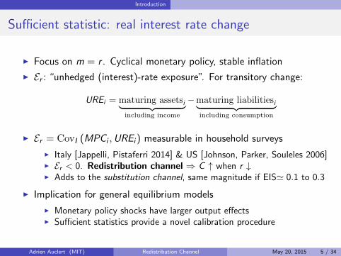
I Focus on m = r . Cyclical monetary policy, stable inflation

I Er : “unhedged (interest)-rate exposure”.

For transitory change:

UREi = maturing assetsi︸︷︷︸including income

−maturing liabilitiesi︸︷︷︸including consumption

I Er = CovI (MPCi ,UREi ) measurable in household surveys

I Italy [Jappelli, Pistaferri 2014] & US [Johnson, Parker, Souleles 2006]

I Er < 0. Redistribution channel ⇒ C ↑ when r ↓I Adds to the substitution channel, same magnitude if EIS' 0.1 to 0.3

I Implication for general equilibrium models

I Monetary policy shocks have larger output effectsI Sufficient statistics provide a novel calibration procedure


Introduction



I Er : “unhedged (interest)-rate exposure”. For transitory change:









Introduction












Introduction







I Italy [Jappelli, Pistaferri 2014] & US [Johnson, Parker, Souleles 2006]I Er < 0. Redistribution channel ⇒ C ↑ when r ↓

I Adds to the substitution channel, same magnitude if EIS' 0.1 to 0.3




Introduction







I Italy [Jappelli, Pistaferri 2014] & US [Johnson, Parker, Souleles 2006]I Er < 0. Redistribution channel ⇒ C ↑ when r ↓I Adds to the substitution channel, same magnitude if EIS' 0.1 to 0.3




Introduction







I Italy [Jappelli, Pistaferri 2014] & US [Johnson, Parker, Souleles 2006]I Er < 0. Redistribution channel ⇒ C ↑ when r ↓I Adds to the substitution channel, same magnitude if EIS' 0.1 to 0.3




Introduction

Dynamic general equilibrium model

I GE model calibrated to U.S. economy matches Er and predicts:

1. Er more negative when assets and liabilities have shorter maturities

I If U.S. only had adjustable rate mortgages, surprise rate changewould more than double current effect

I Cross-country S-VAR evidence [Calza, Monacelli, Stracca 2013]

2. Interest rate increases and cuts have asymmetric effects

I r ↑ lowers output more than r ↓ increases itI [Cover 1992, de Long Summers 1988, Tenreyro Thwaites 2013]I Here: asymmetric response of borrowers close to their credit limits


Introduction









Introduction









Introduction

Limits of analysis

I Framework that accommodates

I HeterogeneityI Nominal and real financial assets of arbitrary durationI Precautionary savings, borrowing constraints

I Abstracts away from

I Risk premiaI RefinancingI Illiquidity and cash holdingsI Collateral price effects on borrowing constraints


Introduction

Related literature

I Monetary policy and redistribution [empirics]

I Inflation: Doepke and Schneider (2006)I Earnings: Coibion, Gorodnichenko, Kueng, Silvia (2012)I Consumption effects: Di Maggio, Kermani, Ramcharan (2014); Keys,

Piskorski, Seru and Yao (2014)

I Monetary policy shocks and the transmission mechanism [theory]

I Christiano, Eichenbaum, Evans (1999, 2005), ...I Role of mortgage structure: Calza, Monacelli, Stracca (2013), Rubio

(2011), Garriga, Kydland and Sustek (2013)I Heterogenous effects : Gornemann, Kuester and Nakajima (2014)

I MPC heterogeneity [theory and empirics]

I Measurement, comovement with balance sheets: Johnson et al (2006),Parker et al (2013), Mian, Rao, Sufi (2013), Baker (2013), ...

I Aggregate demand effects: Galı, Lopez-Salido, Valles (2007),Eggertsson-Krugman (2012), Mian-Sufi (2014), Farhi-Werning (2013)

I Role of incomplete markets: Guerrieri-Lorenzoni (2012), Oh-Reis (2013),Sheedy (2014), McKay-Reis (2014)


Introduction

Outline

1 Partial equilibrium: Er as sufficient statisticPrice theoryIncomplete marketsAggregation

2 Measuring Er

3 General equilibrium model


Partial equilibrium: Er as sufficient statistic Price theory

Outline


2 Measuring Er




Perfect foresight, no uncertainty

I Single agent

I arbitrary non-satiable preferences and time horizonI earns a stream of real income {yt} and wages {wt} (certain)I faces real term structure {tqt+s}s≥1I holds long-term real assets: {t−1bt+s}s≥0 (TIPS, PLAM)

I Date-0 holdings: {−1bt+s}s≥0, term structure qt = (0qt)

I Solves:

I → Initial balance sheet composition irrelevant conditional on W F

I Mortgage M: ARM −1b0 = −M ⇔ PLAM −1bt = −m if∑T

t=0 qtm = M




I Single agent



I Solves:

max U ({ct , nt})s.t. ct = yt + wtnt + (t−1bt) +

∑s≥1

(tqt+s) (t−1bt+s − tbt+s)



t=0 qtm = M




I Single agent



I Solves:

max U ({ct , nt})s.t. ct = yt + wtnt + (t−1bt) +

∑s≥1

(tqt+s) (t−1bt+s − tbt+s)



t=0 qtm = M




I Single agent



I Solves:

max U ({ct , nt})s.t.

∑t≥0

qtct =∑t≥0

qt (yt + wtnt) +∑t≥0

qt (−1bt)︸︷︷︸Financial wealth W F



t=0 qtm = M




I Single agent



I Solves:


∑t≥0

qtct =∑t≥0





t=0 qtm = M




I Single agent



I Solves:


∑t≥0

qtct =∑t≥0





t=0 qtm = M



Unexpected shock


∑t≥0

qtct =∑t≥0

qt (yt + wtnt + (−1bt)) ≡W

I t = 0 → unexpected one-time shock to the real term structure ( dq0

q0= dr)

I First-order change in consumption dc0?

I Composition of balance sheet matters: e.g. “hedged” when



Unexpected shock


∑t≥0

qtct =∑t≥0



q0= dr)


dc0 '∂c0

∂W· (y0 + w0n0 + (−1b0)− c0) dr︸︷︷︸

Wealth effect

+ dch0︸︷︷︸

Substitution effect




Unexpected shock


∑t≥0

qtct =∑t≥0



q0= dr)


dc0 '∂c0

∂W· (y0 + w0n0 + (−1b0)− c0) dr︸︷︷︸

Wealth effect

+ dch0︸︷︷︸

Substitution effect

I Welfare change dU ' Uc0 · (y0 + w0n0 + (−1b0)− c0) dr




Unexpected shock


∑t≥0

qtct =∑t≥0



q0= dr)


dc0 '∂c0

∂W· (y0 + w0n0 + (−1b0)− c0) dr︸︷︷︸

Wealth effect

+ dch0︸︷︷︸

Substitution effect

I Welfare change dU ' Uc0 · (y0 + w0n0 + (−1b0)− c0) dr


−1b0 = c0 − (y0 + w0n0) ∀t



Unexpected shock


∑t≥0

qtct =∑t≥0



q0= dr)


dc0 '∂c0

∂W·

−1URE0︷︸︸︷(y0 + w0n0 + (−1b0)− c0) dr + dch

0︸︷︷︸Substitution effect

I Welfare change dU ' Uc0 · (−1URE0) dr


−1b0 = c0 − (y0 + w0n0) ∀t → −1URE0 = 0



Unexpected shock


∑t≥0

qtct =∑t≥0



q0= dr)


dc0 '

MPC︷︸︸︷∂c0

∂y0·

−1URE0︷︸︸︷(y0 + w0n0 + (−1b0)− c0) dr + dch

0︸︷︷︸Substitution effect

I Welfare change dU ' Uc0 · (−1URE0) dr


−1b0 = c0 − (y0 + w0n0) ∀t → −1URE0 = 0



Unhedged interest rate exposure

URE ≡ −1URE0 =

maturing assets︷︸︸︷y0 + w0n0 + (−1b0) − c0︸︷︷︸

maturing liabilities

I When all financial wealth W F has short maturity:

I URE = y + wn + W F − cI Holder of short-term assets tends to gain when r rises

I One-time dr change, generic U

dc0 = MPC · URE · dr + dch0

I σ ≡ − Uc

cUcclocal EIS

I NNP ≡∑

t≥0 Qt (−1Bt) net nominal position




URE ≡ −1URE0 =





I One-time dr change, time-separable∑βtU (ct , nt)

dc = MPC · URE · dr−σc (1−MPC ) dr

I σ ≡ − Uc

cUcclocal EIS

I NNP ≡∑





URE ≡ −1URE0 =





I One-time dr change, time-separable∑βtU (ct , nt) + date-0 income dy

dc = MPC (dy + UREdr)− σc (1−MPC ) dr

I σ ≡ − Uc

cUcclocal EIS

I NNP ≡∑





URE ≡ −1URE0 =





I + permanent change in price level dP (w/ nominal assets)

dc = MPC

(dy + UREdr − NNP

dP

P

)− σc (1−MPC ) dr

I σ ≡ − Uc

cUcclocal EIS

I NNP ≡∑



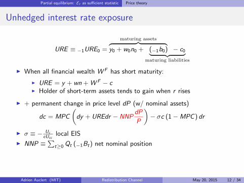
Partial equilibrium: Er as sufficient statistic Incomplete markets

Outline


2 Measuring Er




Incomplete markets, idiosyncratic risk

I Assume now incomplete markets with idiosyncratic uncertainty on {yt ,wt}I Nominal bonds with geometric-decay coupon Λt , rate δNI Perfect foresight over nominal bond price Qt and price level Pt

max E

[∑t

βtU (ct , nt)

]

Ptct = Ptyt + Ptwtnt + Λt + Qt (δNΛt − Λt+1)

Λt+1 ≥ −Ptλ

I Define net nominal position NNPt and unhedged interest rate exposure

NNPt ≡ (1 + QtδN)Λt

Pt

UREt ≡ yt + wtnt +Λt

Pt− ct =

Qt

Pt(Λt+1 − δNΛt)



Individual consumption response: one-time change

I Inelastic labor supply n

I At time 0: permanent increase in price level dP, purely transitory changein income dY = dy + ndw and the real interest rate dr = − dQ

Q

Sufficient statistics for consumption response to transitory shocks

To first order, the consumption response at date 0 is given by

dc ' MPC

(dY + UREdr − NNP

dP

P


where MPC = ∂c∂y is the consumption response to a one-time transitory income

shock (MPC=1 if constrained) and σ = − Uc

cUccis the local EIS

I Logic: consumer is at an interior optimum → behaves identically withrespect to all changes in his balance sheet (or borrowing limit adapts)

I Extensions: elastic labor supply, trees with dividends, ...






Q



dc ' MPC

(dY + UREdr − NNP

dP

P












Q



dc ' MPC

(dY + UREdr − NNP

dP

P








Partial equilibrium: Er as sufficient statistic Aggregation

Outline


2 Measuring Er




Aggregation: environment

I Environment:I Closed economy with no governmentI i = 1 . . . I heterogenous agents (date-0 income Yi = yi + wini )I All participate in financial markets and face the same prices

I Aggregate up (transitory shock, here inelastic labor supply)

dci ' MPCi

(dYi + UREidr − NNPi

dP

P

)− σici (1−MPCi ) dr

I Markets clear at date 0:I Goods

C ≡∑i

ci =∑i

Yi ≡ Y ⇒∑i

UREi = 0

I Assets (here all nominal) ∑i

NNPi = 0



Aggregation: environment

I Environment:I Closed economy with no governmentI i = 1 . . . I heterogenous agents (date-0 income Yi = yi + wini )I All participate in financial markets and face the same prices

I Aggregate up (transitory shock, here inelastic labor supply)

dci ' MPCi

(dYi + UREidr − NNPi

dP

P

)− σici (1−MPCi ) dr

I Markets clear at date 0:I Goods

C ≡∑i

ci =∑i

Yi ≡ Y ⇒∑i

UREi = 0

I Assets (here all nominal) ∑i

NNPi = 0



Aggregation with heterogeneity

Aggregate consumption response to transitory shock

dC '(∑

i

Yi

YMPCi

)dY︸︷︷︸

Aggregate income channel

+ CovI

(MPCi , dYi − Yi

dY

Y

)︸︷︷︸Earnings heterogeneity channel

−CovI (MPCi ,NNPi )︸︷︷︸Fisher channel

dP

P

+

CovI (MPCi ,UREi )︸︷︷︸Interest rate exposure channel

−∑i

σi (1−MPCi ) ci︸︷︷︸Substitution channel

dr

I Logic of Keynesian model: “dC = dY ” given dr

I Two sources of “first-round” effects of r ↓ on consumption

I Second-round effects: income and price adjustment

I With representative-agent (New-Keynesian model), fixed point is

dC = −σCdr



Aggregation with heterogeneity

Aggregate consumption response to transitory shock

dC

C' EI

[Yi

YMPCi

]︸︷︷︸

M

dY

Y+ CovI

(MPCi ,

dYi − YidYY

EI [ci ]

)︸︷︷︸

dEh

−CovI

(MPCi ,

NNPi

EI [ci ]

)︸︷︷︸

EP

dP

P

+

CovI

(MPCi ,

UREi

EI [ci ]

)︸︷︷︸

Er

−σ EI

[(1−MPCi )

ciEI [ci ]

]︸︷︷︸

S

dr

I σ: weighted average of σi

I M, EP , Er and S are measurable

I do not depend on the source of the shockI do not require identification (except for MPC)

I dE h more complex



Focus on slope term

dC

C'MdY

Y+ dE h + EP

dP

P+ (Er − σS) dr

I Next: go to data, find Er = CovI

(MPCi ,

UREi

EI [ci ]

)< 0

I compare to σ using σ∗ = −ErS

I But: usually, in household data EI [UREi ] > 0. Why?

I Maturity mismatch in the household sector (counterpart of banks)I Government with flow borrowing requirements (negative URE)I My benchmark: “Ricardian view” (uniform rebate). Er still correct.

I If none of the gains are rebated: ENRr = EI

[MPCi

UREi

EI [ci ]

]

I ENRr − σS > 0?

“Interestingly [...] low rates could even hurt overall spending”

Raghuram Rajan, November 2013



Focus on slope term

dC

C'MdY

Y+ dE h + EP

dP

P− S (σ∗ + σ) dr


(MPCi ,

UREi

EI [ci ]

)< 0

I compare to σ using σ∗ = −ErS

I But: usually, in household data EI [UREi ] > 0. Why?



[MPCi

UREi

EI [ci ]

]

I ENRr − σS > 0?





Focus on slope term

dC

C'MdY

Y+ dE h + EP

dP

P− S (σ∗ + σ) dr


(MPCi ,

UREi

EI [ci ]

)< 0

I compare to σ using σ∗ = −ErSI But: usually, in household data EI [UREi ] > 0. Why?



[MPCi

UREi

EI [ci ]

]

I ENRr − σS > 0?





Focus on slope term

dC

C'MdY

Y+ dE h + EP

dP

P− S (σ∗ + σ) dr


(MPCi ,

UREi

EI [ci ]

)< 0




[MPCi

UREi

EI [ci ]

]

I ENRr − σS > 0?





Focus on slope term

dC

C'MdY

Y+ dE h + EP

dP

P+(ENRr − σS

)dr


(MPCi ,

UREi

EI [ci ]

)< 0




[MPCi

UREi

EI [ci ]

]I ENRr − σS > 0?





Focus on slope term

dC

C'MdY

Y+ dE h + EP

dP

P+(ENRr − σS

)dr


(MPCi ,

UREi

EI [ci ]

)< 0




[MPCi

UREi

EI [ci ]

]I ENRr − σS > 0?




Measuring Er

Outline


2 Measuring Er



Measuring Er

Map to data

1. Construct a URE measure at the household level

UREi = Yi − Ci + Bi − Di

I Yi : income from all sourcesI Ci : consumption (incl. durables, mtge paymts, excl. house purchase)I Bi : maturing asset stocks (especially deposits)I Di : maturing liability stocks (adjustable rate mortgages, cons. credit)

2. Use a procedure to evaluate MPCi at the household or group level

I Italy Survey of Household Income and Wealth 2010

I Survey measure [Jappelli Pistaferri 2014] Question

I US Consumer Expenditure Survey 2001-2002

I Estimate from randomized receipts of tax rebates [JPS 2006] Details

3. Estimate Er , S , σ∗ = −ErS and ENRrSummary Statistics


Measuring Er

Both surveys and methods show that Er < 0.3

.4.5

.6.7

Ave

rag

e M

PC

in

ce

ntile

−5.67 .03 .26 .59 1.15 11.44Normalized URE: centile mean

MPC vs URE: Italian data grouped by URE centile

−.2

0.2

.4.6

.8E

stim

ate

d M

PC

in

gro

up

−1.03 [−0.54] 0.17 [0.13] 3.00 [1.40]Normalized URE: group mean [median]

MPC vs URE : CEX tax rebate estimation

⇒ Er = CovI

(MPCi ,

UREi

EI [ci ]

)< 0


Measuring Er

Italian data estimation

I Household-level information on MPC and URE : compute directly

Er = CovI

(MPCi ,

UREi

EI [ci ]

)S = EI

[(1−MPCi )

ci

EI [ci ]

]ENRr = EI

[MPCi

UREi

EI [ci ]

]

Time Horizon Annual

Parameter Estimate 95% C.I.

Redistribution elasticity Er -0.06 [-0.09; -0.04]

Hicksian scaling factor S 0.55 [0.53; 0.57]

Equivalent EIS σ∗ = − ErS

0.12 [0.06; 0.17]

No-rebate elasticity ENRr 0.21 [0.17; 0.23]

All statistics computed using survey weights


Measuring Er

CEX data estimation from JPS

I Run MPC estimation over J = 3 groups of URE and compute:

ENRr = EJ

[MPCj

UREj

EI [ci ]

]Er = CovJ

(MPCj ,

UREj

EI [ci ]

)S = EJ

[(1−MPCj

)]Consumption measure Food

Parameter Estimate 95% C.I.

Redistribution elasticity Er -0.24 [-0.42; -0.07]

Hicksian scaling factor S 0.82 [0.69; 0.95]

Equivalent EIS σ∗ = − ErS

0.30 [0.05; 0.54]

No-rebate elasticity ENRr -0.12 [-0.27; 0.02]

Confidence intervals are bootstrapped by resampling households 100 times with replacement


General equilibrium model

Outline


2 Measuring Er





I Objectives

I Propose a rationale for sign and magnitude of Er and σ∗ in the dataI Understand the role of (mortgage) market structureI Evaluate the aggregate effect of persistent shocksI Explore non-linearities in economy’s response

I Model is stylized

I “ARM” experiment only illustrativeI Earnings heterogeneity (dE h) not disciplined by dataI Unexpected shock



Preferences and production

I Measure 1 of households i with GHH preferences:

E

[ ∞∑t=0

(βit)t

u(c it − v

(nit

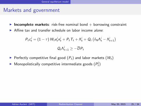
))]I CES in net consumption σ, constant elasticity of labor supply ψ

I All uncertainty is purely idiosyncraticI Idiosyncratic productivity process Πe (e′|e)I Independent discount factor process Πβ (β′|β)I Aggregate state s = (e, β) is in its stationary distribution

I Two-tiered production:I Measure 1 of intermediate good firms, identical linear production

x jt = At l

jt = At

∫i

e itn

i,jt di

I Final good Yt : aggregator of x jt , elasticity ε



Markets and government

I Incomplete markets: risk-free nominal bond + borrowing constraint

I Affine tax and transfer schedule on labor income alone:

Ptcit = (1− τ) Wte

itn

it + PtTt + Λi

t + Qt

(δNΛi

t − Λit+1

)QtΛ

it+1 ≥ −DPt

I Perfectly competitive final good (Pt) and labor markets (Wt)

I Monopolistically competitive intermediate goods (P jt )

I Government collects all profits, runs a balanced budget with no debt

PtTt =

∫j

[P jtx j

t −Wt ljt

]dj + τ

∫i

Wteitn

itdi

I No external supply of assets: market clearing∫iQtΛ

it+1di = 0



Markets and government

I Incomplete markets: risk-free nominal bond + borrowing constraint

I Affine tax and transfer schedule on labor income alone:

Ptcit = (1− τ) Wte

itn

it + PtTt + Λi

t + Qt

(δNΛi

t − Λit+1

)QtΛ

it+1 ≥ −DPt

I Perfectly competitive final good (Pt) and labor markets (Wt)

I Monopolistically competitive intermediate goods (P jt )

I Government collects all profits, runs a balanced budget with no debt

PtTt =

∫j

[P jtx j

t −Wt ljt

]dj + τ

∫i

Wteitn

itdi

I No external supply of assets: market clearing∫iQtΛ

it+1di = 0



Steady-state neutrality of maturity structure

Maturity neutrality

The flexible-price steady state (constant productivity A, constantinflation rate Π = 1, constant gross debt limit D) is invariant to δN

I Constant term structure of interest rates

I → short and long-term assets span the same set of contingencies

I Unhedged interest rate exposures

URE it ≡ (1− τ)

Wt

Pte itn

it + Tt +

Λit

Pt− c i

t

vary with maturity structure, but are refinanced at constant R

I Change δN → change average duration of assets, leave all else equal

I Experiment: Calibrate δN to U.S. then set δN = 0: “only ARMs”



Calibration

I Calibration: quarterly frequency

I Targets:

I Annual eqbm. R = 3% and debt/PCE ratio of 113% (U.S. 2013)I Asset/liability duration of 4.5 years (from Doepke-Schneider)I Y = C = 1 and E [n] = 1I Average quarterly MPC = 0.25

I Parameters:

I Time preference process Πβ : patient (βP)4 = 0.97/imp. (βI )4 = 0.82

I 50% of impatient agentsI Average state duration of 50 years

I Elasticity of labor supply ψ = 1I Elasticity of substitution in net consumption σ = 0.5I Asset/liability coupon decay rate δN = 0.95I Borrowing limit as fraction of average consumption D = 185%I Productivity discretized AR(1), ρ = 0.95 and τ∗ = 0.4 Details



Calibration

I Calibration: quarterly frequency

I Targets:

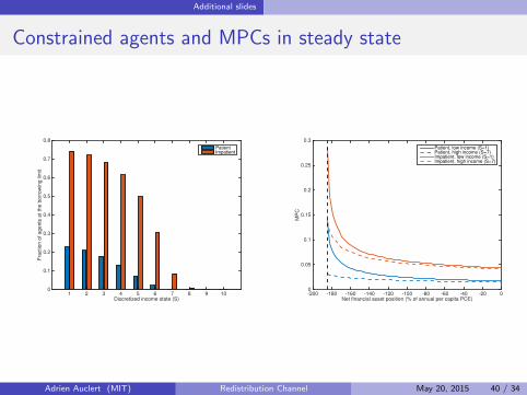
I Annual eqbm. R = 3% and debt/PCE ratio of 113% (U.S. 2013)I Asset/liability duration of 4.5 years (from Doepke-Schneider)I Y = C = 1 and E [n] = 1I Average quarterly MPC = 0.25

I Parameters:

I Time preference process Πβ : patient (βP)4 = 0.97/imp. (βI )4 = 0.82

I 50% of impatient agentsI Average state duration of 50 years

I Elasticity of labor supply ψ = 1I Elasticity of substitution in net consumption σ = 0.5I Asset/liability coupon decay rate δN = 0.95I Borrowing limit as fraction of average consumption D = 185%I Productivity discretized AR(1), ρ = 0.95 and τ∗ = 0.4 Details



Redistribution channel in the model

I For transitory monetary policy shock, can show:

dC

C'MdY

Y+ dE h︸︷︷︸EY dY

Y

+EPdP

P− S (σ∗ + σ) dr +T dY

Y︸︷︷︸Complementarity channel

Steady-state valueDetails and compare to data δN = 0.95 δN = 0

U.S. “Only ARMs”

Redistribution elasticity for r Er −0.09

−1.76

Hicksian scaling factor S 0.57

Equivalent EIS σ∗ = −ErS 0.15

3

Income weighted MPC M 0.16

Earnings heterogeneity factor EY −0.09

Redistribution elasticity for P EP 1.77

Consumption-labor compl. term T 0.46



Redistribution channel in the model

I For transitory monetary policy shock, can show:

dC

C'MdY

Y+ dE h︸︷︷︸EY dY

Y

+EPdP

P− S (σ∗ + σ) dr +T dY

Y︸︷︷︸Complementarity channel

Steady-state valueDetails and compare to data δN = 0.95 δN = 0

U.S. “Only ARMs”

Redistribution elasticity for r Er −0.09 −1.76

Hicksian scaling factor S 0.57

Equivalent EIS σ∗ = −ErS 0.15 3

Income weighted MPC M 0.16

Earnings heterogeneity factor EY −0.09

Redistribution elasticity for P EP 1.77

Consumption-labor compl. term T 0.46



Sticky prices

I In a steady-state, suppose prices are fully sticky: Pt = Pt−1

I Central bank stabilizes, nominal interest rate = steady-state R

I Replicates the flexible-price allocation

I Monetary policy shock: unexpectedly lowers the nominal rate

Rt = ρRt−1 + (1− ρ) R − εt

I Fisher channel is shut down

I Full nonlinear solution keeping track of wealth distribution

I find sequence {wt} ensuring market clearing Ct = Yt

I Borrowing limits keep real value of payments next period fixed Details



Sticky prices

I In a steady-state, suppose prices are fully sticky: Pt = Pt−1

I Central bank stabilizes, nominal interest rate = steady-state R

I Replicates the flexible-price allocation

I Monetary policy shock: unexpectedly lowers the nominal rate

Rt = ρRt−1 + (1− ρ) R − εt

I Fisher channel is shut down

I Full nonlinear solution keeping track of wealth distribution

I find sequence {wt} ensuring market clearing Ct = Yt

I Borrowing limits keep real value of payments next period fixed Details



Transitory monetary policy easing

Time in quarters-1 0 1 2 3 4 5 6 7 8 9 10

Per

cent devia

tion fro

m s

teady-s

tate

-0.4

-0.2

0

0.2

0.4

0.6

0.8

1

1.2

1.4Transitory monetary policy shock (persistence=0)

Real interest rate impulseOutput response: US calibrationOutput response: representative agentt=0 predicted values from sufficient statistic



Transitory monetary policy easing

Time in quarters-1 0 1 2 3 4 5 6 7 8 9 10

Per

cent devia

tion fro

m s

teady-s

tate

-0.4

-0.2

0

0.2

0.4

0.6

0.8

1

1.2

1.4Transitory monetary policy shock (persistence=0)

Real interest rate impulseOutput response: US calibrationOutput response: Only ARMsOutput response: representative agentt=0 predicted values from sufficient statistic



Prolonged monetary policy easing

Time in quarters-1 0 1 2 3 4 5 6 7 8 9 10

Per

cent devia

tion fro

m s

teady-s

tate

-0.4

-0.2

0

0.2

0.4

0.6

0.8

1

1.2

1.4

1.6Persistent monetary policy shock (persistence=0.5)

Real interest rate impulseOutput response: US calibrationOutput response: Only ARMsOutput response: representative agent



Asymmetric effects

1-quarter change in real interest rate (basis points, annualized)-500 -400 -300 -200 -100 0 100 200 300 400 500

Perc

enta

ge c

hange in

outp

ut

-8

-6

-4

-2

0

2

4

6

8Effect on output of a change in r (General Equilibrium)

US benchmark calibrationFirst-order approx.ARM-only calibrationFirst-order approx.


Conclusion

Conclusion

I Monetary policy redistributes:

I One reason why it affects aggregate consumptionI Likely to be the dominant one in ARM countriesI Sufficient statistics, Em = CovI

(MPCi ,Exposurei,m

), establish orders

of magnitude and discipline model calibrations

I Implications for mortgage market design and monetary policy:

I Capital gains can act against MPC-aligned redistributionI The effects of monetary policy may vary (with Er ) over the cycleI Redistribution elasticities, tracked through household surveys, can

inform monetary policy decisions


Additional slides

Thank you!


Additional slides

SHIW MPC question

I In the 2010 survey [analyzed by Jappelli and Pistaferri 2014]

Imagine you unexpectedly receive a reimbursement equal to the amount your householdearns in a month. How much of it would you save and how much would you spend?Please give the percentage you would save and the percentage you would spend.

I In the 2012 survey

Imagine you receive an unexpected inheritance equal to your household’s income for ayear. Over the next 12 months, how would you use this windfall? Setting the totalequal to 100, divide it into parts for three possible uses:

1. Portion saved for future expenditure or to repay debt (MPS)

2. Portion spent within the year on goods and services that last in time (jewelleryand valuables, motor vehicles, home renovation, furnishing, dental work, etc.)that otherwise you would not have bought or that you were waiting to buy(MPD)

3. Portion spent during the year on goods and services that do not last in time(food, clothing, travel, holidays, etc.) that ordinarily you would not have bought(MPC)

Back


Additional slides

Johnson, Parker, Souleles (2006) tax rebates

I Sort all households into J quantiles of URE

I Run main estimating equation from JPS:

Ci,m,t+1 − Ci,m,t = αm + βXi,t +J∑

j=1

MPCjRi,t+1QUREi,j + ui,t+1

I Ci,m,t : level of i ’s consumption expenditure in month m and date tI Xi,t : age and family compositionI Ri,t+1: dollar amount of the rebate receiptI QUREi,j = 1 if household i ∈ interest rate exposure group MPCj

I Estimation of MPCj exploits randomized variation in timing of receipt oftax rebate among households in URE group j

Back


Additional slides

Datasets: summary statistics

SHIW 2010 CEX 2001

Variable mean n.s.d. mean n.s.d.

Income from all sources (Yi , per year) 36,114 0.90 45,617 1.01

Consumption incl. mortgage payments (Ci , per year) 27,976 0.61 36,253 0.79

Deposits and maturing assets (Bi ) 14,200 1.45 7,147 0.77

ARM mortgage liabilities and consumer credit (Di ) 6,228 1.03 2,872 0.22

Unhedged interest rate exposure (UREi , per year) 16,110 1.92 13,639 1.27

Unhedged interest rate exposure (UREi , per Q) 10,007 7.07 6,616 3.39

Marginal Propensity to Spend (annual) 0.47 0.35

Count 7,951 9,443

“mean”: sample mean computed using sample weights (in BC for SHIW; current USD for CEX)

“n.s.d”: normalized standard deviation, sdI

(Xi

EI [Ci ]

)for Xi = Yi , Ci , Bi ,UREi and sdI (MPCi ) for MPC

Back


Additional slides

Calibration (continued)

I Idiosyncratic productivity process: discretized AR(1)

log et = ρ log et−1 + σe√

1− ρ2εt εt ∼ N (0, 1)

I Lognormal stationary distribution of pre-tax earnings, var. σ2e (1 + ψ)2

I Set σe (1 + ψ) = 1.04 to empirical counterpart in 2009 PSIDI τ∗ = 0.4 matches typical calibration for (post-tax) earningsI Moderate persistence level: ρ = 0.95 (quarterly) Back

Cumulative population proportion0 0.1 0.2 0.3 0.4 0.5 0.6 0.7 0.8 0.9 1

Cum

ula

tive labor

earn

ings p

roport

ion

0

0.1

0.2

0.3

0.4

0.5

0.6

0.7

0.8

0.9

1

PSID 2009 Pre-tax labor earnings distributionModel pre-tax labor earningsModel post-tax&transfer labor earningsModel post-tax&transfer net labor earningsTypical calibration (variance of log earnings=0.6)Perfect equality line


Additional slides

Constrained agents and MPCs in steady state

Discretized income state (S)1 2 3 4 5 6 7 8 9 10

Fra

ction o

f agents

at th

e b

orr

ow

ing lim

it

0

0.1

0.2

0.3

0.4

0.5

0.6

0.7

0.8

PatientImpatient

Net financial asset position (% of annual per capita PCE)-200 -180 -160 -140 -120 -100 -80 -60 -40 -20 0

MP

C

0

0.05

0.1

0.15

0.2

0.25

0.3

Patient, low income (S=1)Patient, high income (S=7)Impatient, low income (S=1)Impatient, high income (S=7)


Additional slides

Redistribution elasticity Er in the model and in data

Asset/Liability duration in years0 0.5 1 1.5 2 2.5 3 3.5 4 4.5 5

Er

-1.8

-1.6

-1.4

-1.2

-1

-0.8

-0.6

-0.4

-0.2

0

Redistribution elasticity in modelBenchmark calibrationItaly: SHIW dataUS CEX: Food estimateUS CEX: All nondurable

Back


Additional slides

Other moments

I Construct counterpart to QΛ: net interest-paying assets (Deposits,IRAs and other assets minus all debts)

Mean sd P5 P25 Median P75 P95 P99

QΛE[c]

PSID 2009 1.17 32.51 -28.42 -6.88 0.00 1.78 35.86 113.90

Model 0 17.96 -7.4 -7.27 -6.11 0.32 25.96 54.05

Units: average quarterly consumption


Additional slides

Transition after shocks

I Debt limit maintains next period real coupon payments fixed:

Dt = Qtd ⇔ λt+1 ≥ −d

I When Πt = 1, B.C. of agents at the borrowing limit:

c it = y i

t−

d +Qt

Q×(−D (1− δN)

)︸︷︷︸URE

Steady-state value

δN = 0.95 δN = 0

min{

y i}

0.413 0.413

d 0.413 7.455

URE −0.358 −7.400

(R − 1) D 0.055 0.055

Back


Additional slides

Monetary policy and the redistribution channels

Monetary accomodation Real interest rate ↓ Aggregate demand ↑

Aggregate income ↑

Individual incomes ↑

Substitution

AggregateMPC

Standard New-Keynesian model (fully sticky prices)

Back


Additional slides





Substitution

Interest-rateexposure

AggregateMPC


Redistribution channels

Back


Additional slides





Substitution


AggregateMPC

Earningsheterogeneity



Back


Additional slides




Hours worked ↑


Substitution


AggregateMPC

Complementarity

Earningsheterogeneity


Consumption/labor complementarities


Back


Date post:	30-Mar-2018
Category:	Documents
Upload:	vuonglien
View:	220 times
Download:	2 times

Monetary Policy and the Redistribution Channel · PDF fileMonetary Policy and the...

Documents