Money and Banking

Lecture V: Empirical Methods for Research on Money and Finance

Guoxiong ZHANG, Ph.D.

Shanghai Jiao Tong University, Antai

October 16th, 2018

Why Identification is Important

Source: http://econjeff.blogspot.com

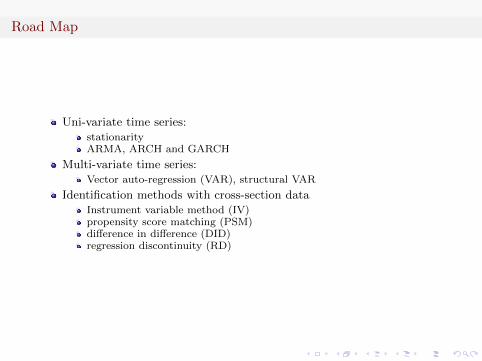
Road Map

Uni-variate time series:stationarityARMA, ARCH and GARCH

Multi-variate time series:Vector auto-regression (VAR), structural VAR

Identification methods with cross-section dataInstrument variable method (IV)propensity score matching (PSM)difference in difference (DID)regression discontinuity (RD)

Stationarity: definition

A time series is stationary if it has a time-invariant and finite mean,variance and auto-covariance:

E(xt) = E(xt−j) = µ, ∀j;

var(xt) = var(xt−j) = σ2, ∀j;

cov(xt, xt−j) = η2j , ∀t.

Stationarity is necessary for meaningful econometric analysis:economists are mostly interested in cycles instead of trends;variance of the error term can be unrealistically large, which makesstatistical inference meaningless

By stationarity we can classify uni-variate time series into three types:stationarydeterministic trendsunit root (stochastic trends)

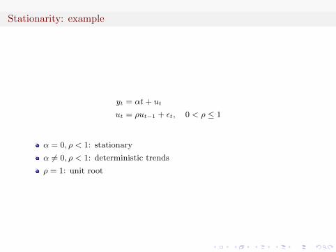
Stationarity: example

yt = αt+ ut

ut = ρut−1 + εt, 0 < ρ ≤ 1

α = 0, ρ < 1: stationary

α 6= 0, ρ < 1: deterministic trends

ρ = 1: unit root

Stationarity: example

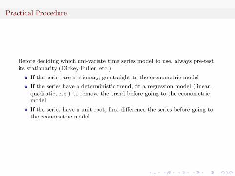
Practical Procedure

Before deciding which uni-variate time series model to use, always pre-testits stationarity (Dickey-Fuller, etc.)

If the series are stationary, go straight to the econometric model

If the series have a deterministic trend, fit a regression model (linear,quadratic, etc.) to remove the trend before going to the econometricmodel

If the series have a unit root, first-difference the series before going tothe econometric model

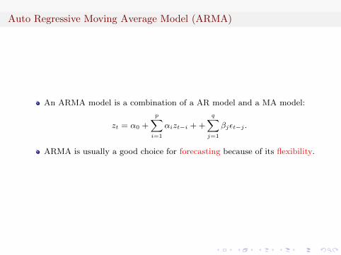
Auto Regressive Moving Average Model (ARMA)

An ARMA model is a combination of a AR model and a MA model:

zt = α0 +

p∑i=1

αizt−i + +

q∑j=1

βjεt−j .

ARMA is usually a good choice for forecasting because of its flexibility.

ARCH and GARCH Model

yt = γ0 +Xtγ + ut.

where var(ut) = σ2t .

Autoregressive Conditional Heteroskedasticity (ARCH(p)) Model:

σ2t = α0 +

p∑i=1

αiu2t−i.

Generalized Autoregressive Conditional Heteroskedasticity (GARCH(p,q)) Model:

σ2t = α0 +

p∑i=1

αiu2t−i +

q∑j=1

βjσ2t−j .

ARCH and GARCH are useful when dealing with financial time seriesthat have time varying volatility.

Vector Autoregression Model (VAR)

A VAR model is a multi-variate generalization of the ARMA model;

Reduced form VARs are used for estimation and forecasting; StructuralVARs are used for identification;

We start with a structural form example:

yt = αy + αy,0it +

p∑j=1

αyy,jyt−j +

p∑j=1

αiy,jit−j + εy,t

it = αi + αi,0yt +

p∑j=1

αyi,jyt−j +

p∑j=1

αii,jit−j + εi,t

where

E

(εy,tεi,t

)= 0, cov

(εy,tεi,t

)=

(σ2y, 0

0, σ2i

)Direct estimation on the structural VAR is problematic because ofendogeneity.

Vector Autoregression Model (VAR)

In matrix form:(1,−αy,0−αi,0, 1

)(ytit

)=

(αyy,1, α

iy,1

αyi,1, αii,1

)(yt−1

it−1

)+

(αyy,p, α

iy,p

αyi,p, αii,p

)(yt−pit−p

)

+

(εy,tεi,t

)Equivalently:

A0

(ytit

)= A1

(yt−1

it−1

)+ ...+Ap

(yt−pit−p

)+

(εy,tεi,t

)

From Structural Form to Reduced Form

Multiply both sides with A−10 :(

ytit

)= A−1

0 A1

(yt−1

it−1

)+ ...+A−1

0 Ap

(yt−pit−p

)+A−1

0

(εy,tεi,t

)Assume σ2

y = σ2i = 1, then

ut = A−10

(εy,tεi,t

)Σu = A−1

0 A−10

′.

The reduced form is free from endogeneity issue and therefore ready forestimation and forecasting (even OLS equation by equation will begood enough);

However, to perform meaningful economic analysis we have to convertthe estimated reduced form model back to the structural form.

From Reduced Form to Structural Form

From the above reduced form we can only obtain estimates: A−10 A1,

A−10 Ap, and hence ut and Σu.

As long as we can identify A−10 then we can identify Aj , j = 1, ..., p.

However, Σu as a n× n symmetric matrix only have n(n+1)2

elements

while Aj have n2 unknown parameters;

Therefore to obtain the structural VAR we need to impose n(n−1)2

restrictions (one in our example).

Usually these restrictions come from economic theory ( particularordering, sign restriction, etc.)

Impulse Response

Impulse responses are vary useful for policy analysis: how much changean exogenous shock can cause on an endogenous economic variableacross time;

The idea is that an exogenous shock at time t (εi,t) can affect both ytand it at time t, and in turn yt and it affect yt+1 and it+1, and so on; sothe impulse responses are accumulated effects of an exogenous shock;

Formally define A(L) = I − A1L− A2L2 − ...− ApLp (A(0) = I), then

the estimated reduced form can be written as

A(L)Xt = ut, Xt =

(εy,tεi,t

)Then we have

Xt = C(L)εt, C(L) = A(L)−1A−10 ,

and Ci,j(h) is the impulse response of variable i to shock j after hperiods (εt(j)→ Xt+h(i)).

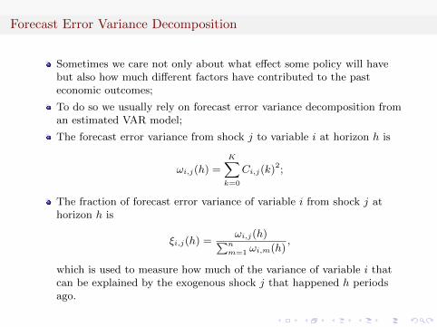
Forecast Error Variance Decomposition

Sometimes we care not only about what effect some policy will havebut also how much different factors have contributed to the pasteconomic outcomes;

To do so we usually rely on forecast error variance decomposition froman estimated VAR model;

The forecast error variance from shock j to variable i at horizon h is

ωi,j(h) =

K∑k=0

Ci,j(k)2;

The fraction of forecast error variance of variable i from shock j athorizon h is

ξi,j(h) =ωi,j(h)∑n

m=1 ωi,m(h),

which is used to measure how much of the variance of variable i thatcan be explained by the exogenous shock j that happened h periodsago.

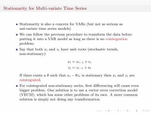
Stationarity for Multi-variate Time Series

Stationarity is also a concern for VARs (but not as serious asuni-variate time series models)

We can follow the previous procedure to transform the data beforeputting it into a VAR model as long as there is no cointegrationproblem;

Say that both xt and zt have unit roots (stochastic trends,non-stationary):

xt = xt−1 + εt

zt = zt−1 + νt

If there exists a θ such that xt − θzt is stationary then xt and zt arecointegrated.

For cointegrated non-stationary series, first differencing will cause evenbigger problem. One solution is to use a vector error correction model(VECM), which has some other problems of its own. A more commonsolution is simply not doing any transformation.

Practical Procedure

select variables for VAR: must have economic meaning, usually threevariables, rarely exceeds five;

decide using level, log level, log difference or HP filter: often using loglevel is the best choice except for data with obvious trend such asChina’s GDP;

determine number of lags p: using BIC or AIC is standard, but usuallyone lag for annual data, four lags for quarterly or monthly data inpractice;

estimate the reduced form VAR

obtain the coefficient for the structural form VAR (most softwares cando this automatically)

perform impulse response and forecast error variance decompositionanalysis

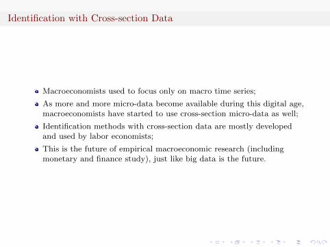
Identification with Cross-section Data

Macroeconomists used to focus only on macro time series;

As more and more micro-data become available during this digital age,macroeconomists have started to use cross-section micro-data as well;

Identification methods with cross-section data are mostly developedand used by labor economists;

This is the future of empirical macroeconomic research (includingmonetary and finance study), just like big data is the future.

Instrument Variable

Consider a standard linear regression model:

yi = Xiβ + ei,

The ordinary least square (OLS) estimator is simply

βOLS = (X′X)−1X

′y = β + (X

′X)−1X

′e.

Endogeneity happens when X and e are correlated and therefore X′e

does not converge to zero in the limit. In this case the βOLS is NOT anunbiased and consistent estimator of β.

The simplest way to solve endogeneity issue is to find one or moreinstrument variables Z for the endogenous variable xj such that

cov(Z, xj) 6= 0 and cov(Z, y) = 0.

Two Stage Least Square (2SLS)

Estimation can be carried out by a 2SLS approach:regress xj on Z and use the estimated coefficient to obtain predicted xj ;replace xj with xj and run the standard OLS regression on the firstequation (leave the good and replace the bad).

Formally the 2SLS estimator is given as

β2SLS = (Z′X)−1Z

′y = (Z

′X)−1Z

′Xβ + (Z

′X)−1Z

′e.

Usually the number of instruments should be no larger than thenumber of endogenous variables; if not, use GMM (a generalized 2SLS,common when using lags as instruments)

classical example: rain fall, economic growth, civil war

Propensity Score Matching

To evaluate a treatment effect medical scientists usually useexperiments to create control group and experiment group andcompare them;

Unfortunately this scientific approach is rarely applicable in economicresearch: it is difficult to find subjects that are identical (orstatistically identical) prior treatment;

Formally an average treatment effect is defined as

ATT ≡ E(Yi1|Di = 1)− E(Yi0|Di = 1);

where Di is the targeting dummy, Yi1 is the outcome with treatmentand Yi0 is the outcome without treatment;

E(Yi0|Di = 1) is of course not observable; the key is to find Xi suchthat

E(Yi0|Di = 1, Xi) = E(Yi0|Di = 0, Xi)

Propensity Score Matching

Find covariates to run a logit or probit regression to predict theprobability that each subject is chosen to be treated (propensity score);

A treated subject is matched with other subjects that have closepropensity score;

Average treatment effect is calculated by comparing the outcomesbetween matched treated and not treated subjects;

PSM has been used extensively, but is far from perfect:using different covariates can give different propensity scores;how close is close enough is still arbitrary.

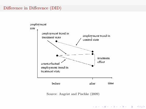
Difference in Difference (DID)

Source: Angrist and Pischke (2009)

Difference in Difference (DID)

The key idea of DID is that assuming treatment group (s=1) andcontrol group (s=2) have common trends:

Yist = αs + λT + βDst + εist

And therefore

β = [E(Yi,s=1,t=1)− E(Yi,s=1,t=0)]− [E(Yi,s=2,t=1)− E(Yi,s=2,t=0)]

Whether the implementation of DID is successful or not depends onthe existence of common trends (control other factors except for thetreatment, e.g. restaurants across the boarder in Card and Krueger(1994)).

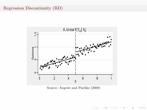
Regression Discontinuity (RD)

Source: Angrist and Pischke (2009)

Regression Discontinuity (RD)

Let ρ be the treatment effect we care about:

Yi = f0(xi)(1−Di) + f1(xi)Di + ρDi + εi

We can use polynomials to approximate f(xi):

E(Y0i|xi) = f0(xi) = α+

p∑j=1

β0j(xi − x0)j

E(Y1i|xi) = f1(xi) = α+

p∑j=1

β1j(xi − x0)j + ρ

Regression Discontinuity (RD)

Then we have the regression equation as

Yi = α+

p∑j=1

β0j(xi − x0)j + ρDi +

p∑j=1

(β1j − β0j)Di(xi − x0)j + εi

In theory this approximation function may not be accurate andtherefore some people like to use non-parametric methods:

limδ→0

[E(Yi|x0 < xi < x0 + δ)− E(Yi|x0 − δ < xi < x0)]

= E(Y1i − Y0i|xi = x0) = ρ

Regression Discontinuity (RD)

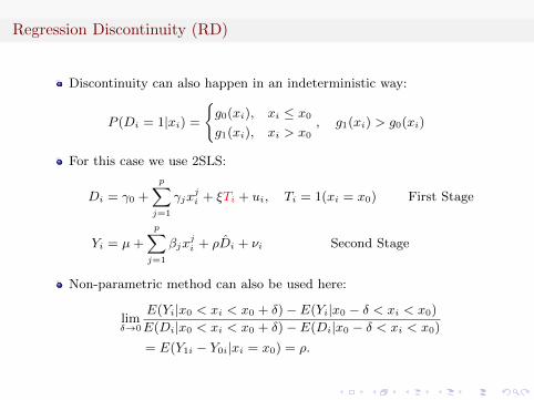
Discontinuity can also happen in an indeterministic way:

P (Di = 1|xi) =

{g0(xi), xi ≤ x0g1(xi), xi > x0

, g1(xi) > g0(xi)

For this case we use 2SLS:

Di = γ0 +

p∑j=1

γjxji + ξTi + ui, Ti = 1(xi = x0) First Stage

Yi = µ+

p∑j=1

βjxji + ρDi + νi Second Stage

Non-parametric method can also be used here:

limδ→0

E(Yi|x0 < xi < x0 + δ)− E(Yi|x0 − δ < xi < x0)

E(Di|x0 < xi < x0 + δ)− E(Di|x0 − δ < xi < x0)

= E(Y1i − Y0i|xi = x0) = ρ.

Be Careful with RD

Source: Angrist and Pischke (2009)