Department of Economics Supervisor: Klas Fregert Lund University August 2011 Master thesis, 15p

Money Illusion and the Optimal Long-

Run Rate of Inflation By

Hannes Stiernstedt

1

Abstract

The conventional NAIRU model stipulates that any existing money illusion would vanish by the

passage of time. In contrast, the model developed by Akerlof, Dickens and Perry (2000) (ADP) argues

that inflation, instead of time, dissipate money illusion. Accordingly, there exists a possibility of an

inflation unemployment tradeoff in the long run. This essay reviews the evidence of money illusion

and the main criticism against the ADP-model. Furthermore, a reevaluation of the Swedish

backward-bending Phillips curve derived by Lundborg and Sacklén (2006) is performed, using an

updated dataset covering a longer time period with an inflation targeting regime. The results are

inconclusive to whether the Phillips curve derived by Lundborg and Sacklén hold in the new time

period, which warrants further analysis.

Keywords: Money Illusion, Phillips curve, efficiency wages, near-rationality

2

Table of Contents

Abstract ................................................................................................................................................... 1

List of Tables and Figures ........................................................................................................................ 3

Tables .................................................................................................................................................. 3

Figures ................................................................................................................................................. 3

1. Introduction ......................................................................................................................................... 4

1.1. Outline of the Essay ...................................................................................................................... 5

2. Money Illusion ..................................................................................................................................... 6

2.1. Evidence of Money Illusion .......................................................................................................... 7

2.2. Effects of Money Illusion .............................................................................................................. 9

3. A New Account on the Long-Run Inflation Unemployment Tradeoff ............................................... 11

3.1. The ADP-Model and the Optimal Unemployment Rate of Inflation .......................................... 11

3.2. Criticism Against the ADP-Model ............................................................................................... 13

4. Theoretical Model ............................................................................................................................. 15

5. Empirical Model and Data Sources .................................................................................................... 19

5.1. Empirical Model .......................................................................................................................... 19

5.2. Data Sources and Variable Construction .................................................................................... 20

6. Results ............................................................................................................................................... 22

6.1. Research Design ......................................................................................................................... 22

6.2. Results from Restricted Optimization ........................................................................................ 23

7. Conclusion ......................................................................................................................................... 29

8. Appendix ............................................................................................................................................ 31

9. References ......................................................................................................................................... 32

3

List of Tables and Figures

Tables

Table 1: Summary statistics……….......................................................................................................….21

Table 2: Summary Table of Estimated Parameter Values.....................................................................23

Figures

Figure 1: Hypothetical Phillips Curve.....................................................................................................17

Figure 2: Inflation vs. Unemployment...................................................................................................21

Figure 3: Long-Run Phillips Curve, i.......................................................................................................24

Figure 4: Long-Run Phillips Curve, ii......................................................................................................24

Figure 5: Long-Run Phillips Curve, iii.....................................................................................................25

Figure 6: Long-Run Phillips Curve, iv.....................................................................................................26

Figure 7: Long-Run Phillips Curve, v......................................................................................................26

Figure 8: Long-Run Phillips Curve, vi.....................................................................................................27

Figure 9: Long-Run Phillips Curve, vii.....................................................................................................28

4

1. Introduction

In standard economic theory, there is a difference between nominal wage rigidities and real wage

rigidities. The former cause cyclical unemployment and the latter is the cause of structural

unemployment. Nominal wage rigidities, or more commonly known as sticky wages, are usually

considered caused by menu costs, fairness concerns, money illusion or imperfect information on

price changes. Real wage rigidities are thought of being caused mainly by efficiency wages and trade

unions.

In the short run, where inflation expectations are pre-determined, there exists a tradeoff between

inflation and unemployment and the sloped short-run Phillips curve is derived. But if actual inflation

deviates from expected inflation, expectations will adjust over time causing a shift in the short-run

Phillips curve. Assuming a positive correlation between past values of inflation and the expected

inflation, inflation will move in opposite direction to unemployment when it is above its natural,

long-run, level. Thus, the non-accelerating inflation rate of unemployment (NAIRU) implies a vertical

Phillips curve (Sørensen, Whitta-Jacobsen, 2010:292,487).

So even if money illusion is admitted to exist in the short run, it is thought to disappear in the long

run as people learn from their mistakes. But theoretical and empirical research on path dependency

in the economy suggests that persistent but transitory changes in aggregate demand may have

permanent effects on output and employment (Fontana and Palacio-Vera, 2007). So from a

theoretical point of view, there are many authors that have created models challenging the standard

NAIRU framework, opening up for the possibility of long-run money non-neutrality. The holy grail of

this research is of course the possibility this creates for monetary policies to affect output and

employment in the long run. Because if changes in aggregate demand, induced by central banks,

affect output in the long run then inflationary policies can in the long run reduce unemployment.

According to Maugeri (2010), the literature on this subject can be divided into two main strands.

There are path dependency models and market imperfections models. The former include demand

led growth models, hysteresis models and multiple equilibria models (Fontana and Palacio-Vera,

2007). Market imperfections models insert some kind of rigidity in the functioning of the labor

market (Maugeri, 2010). In the latter type of research, Akerlof, Dickens and Perry (2000) has created

a model (henceforth the ADP-model) that assumes money illusion in the long run trying to establish a

long-run tradeoff between inflation and unemployment.

This essay aims to review the evidence of money illusion and the case for money non-neutrality in

the long run. This is an important question since long-run money illusion raises the possibility of

partly controlling the level of unemployment via the inflation level. Indeed, if such a relationship is

present, money illusion may be the most important factor to consider when choosing the level of

inflation (Shafir et al. 1997). The ADP-model provides a very intuitive theory that encompasses

money illusion in an efficiency wage setting. Therefore, the main goal of this essay is to replicate the

backward-bending Phillips curve in a Swedish setting. Earlier research has applied the same ADP-

model on few other countries, with mixed results. The most thorough research with the ADP-model,

besides from Akerlof et al. have been made with data from Sweden and Italy. The previous Swedish

study was conducted by Lundborg and Sacklén (2006), using data between the years 1963 and 2000.

5

But there is a case for reviewing the Swedish study. Since the last study, 10 more years of data can be

added to the series. These years are very interesting since the inflation has remained very low and

stable over this last decade. This is due to the adoption of an inflation target in 1993. Consequently,

over 40 per cent of the time period analyzed in this essay is covered by in inflation targeting regime

which has stabilized both the actual inflation rate and inflation expectations around a level that is

very interesting in the ADP-model.

1.1. Outline of the Essay

The essay is organized in the following way. Since the concept of money illusion is central to the ADP-

model, the next chapter introduces money illusion together with a description of the historical

development of the theoretical Phillips curve. The following section describes some of the evidence

of money illusion. The chapter concludes by giving a brief account on how money illusion can affect

the economy. Chapter three introduces the economics behind the ADP-model and the research

concerning the optimal rate of inflation. The chapter also describes previous research that has made

use of the ADP-model, and concludes with a description of the criticism against the ADP-model.

Up to this point, money illusion, being the major theoretical underpinning of the ADP-model, has

been introduced, together with the research done with the use of the ADP-model and the criticism it

has generated. Chapter four provides a theoretical derivation of the model, as derived by Akerlof et

al. (2000). Chapter five describes the empirical model and data sources. Chapter six describes the

research design and the main results. Finally, chapter seven contains concluding remarks.

6

2. Money Illusion

This chapter describes the key features of the concept of money illusion, its evolution, how it is

evident in real life and some effects of money illusion. The first part defines the concept and put it in

a historical context. This is important in order to know that the notion of long-run non-neutrality of

money is nothing new, only the discourse is. Section 2.1 describes some evidence of money illusion in

economic agents while section 2.2 deals with the possible effects of money illusion on an aggregate

level.

Money illusion refers to situations in which people mistake the face value of money for its purchasing

power, when they display a tendency to think in terms of nominal rather than real monetary values.

Through time, the concept has been widely debated and is an intrinsic part of behavioral economics.

In macro economics the concept has been well known for at least a century, and made Irving Fisher

famous when he wrote “Money Illusion” (1928). Fisher defined money illusion as the tendency of

people to think of currency in nominal, rather than real, terms. Later, Keynes (1936:5ff)

acknowledged the phenomenon of non-neutrality of money in his General Theory of Employment

Interest and Money. It was said that workers suffered from money illusion, so that the labor supply

curve depends on the nominal wage rate while the demand curve depends on the real wage.

It is in this central discourse of the concept of money illusion that A. W. Phillips presented his findings

about the relationship between unemployment and inflation in United Kingdom (1958). This original

Phillips Curve has the form (Phillips, 1958:290 and Lipsey, 1960:3f) and allow for

money illusion if . Each per cent increase in inflation, , raises wages, , by , which is less

than unity reducing the real wage which allows for a sloped Phillips curve both in short and long run.

But the central concept of money illusion in long run macro economics died with the 1968 article by

Milton Friedman “The Role of Monetary Policy”. In the article, Friedman denounces the possibility

that the labor supply curve could depend on the nominal wage rate (1968:8). In his view, must

equal to 1. Everything else is fundamentally illogical. Hence, there is no trade of between inflation

and unemployment in the long run. This view became prevalent in decades to come. Some

economists went even further in denouncing money illusion. The Nobel laureate James Tobin wrote

the following in his article “Inflation and Unemployment”: “An economic theorist can, of course,

commit no greater crime than to assume money illusion” (1972:3).

Yet, there were still some proponents of money illusion left, but it took another decade until new

theories fought its way into the spotlight. In 1979, Daniel Kahneman and Amos Tversky presented

their Prospect Theory. The theory describes a number of phenomena, each challenging the

predominant expected utility theory. They meant that, when it comes to decisions under risk, we do

not behave rationally and according to the expected utility theory (1979:263). But it was not until the

well known article by Shafir et al. (1997) that money illusion received some of the attention it once

had. There, they proposed and described a psychological account to the causes of money illusion.

7

2.1. Evidence of Money Illusion

There have been many studies concerning money illusion and the most straightforward are

experiments evaluating people’s reaction to variations in inflation and prices. As a result of these

studies, Shafir et al. proposes that people tend to think of economic transactions both in real and

nominal terms, with a bias toward a nominal evaluation process (1997:341). This is not an

unreasonable proposition. One channel in which this may happen is when people simplify a

representation to make decisions easier. This is what Kahneman and Tversky call editing, stipulating

that people rule out less important information to make better decisions on the factors that matters

the most (1979:274). Maybe it is that items must reach a certain threshold of exposure before being

perceived. Kahneman and Tversky are not alone in stipulating that people tend to simplify their

decision making. Other psychologists view people’s decision making partly in simplified abstract

models. Nisbett and Ross considers behavior like editing be a part of many heuristics creating

irrational behavior originating from cognitive limitations (1980).

Research in cognitive psychology has yielded the conclusion that when people are faced with

alternative representations of the same situation their answer is systematically different (Shafir et

al., 1997:345). This is in accordance to Kahneman and Tverskys (1979) Prospect Theory contradicting

the standard economic model. This is due to the framing of the questions, affecting both time and

risk preferences. If the question if framed in nominal terms, people tend to prefer the nominally less

risky option which is in fact more risky in real terms. This is most likely because nominal options are

simpler, and suffice in short run. It is not that people are not aware of inflation, just that in any point

in time economic transactions are easier to think of in nominal terms. That is why economic decisions

are a mixture of nominal and real assessments, creating effects from money illusion in the economy.

For example, a close to three per cent wage increase in times of six per cent inflation is by many

individuals preferred to a three per cent wage cut in times of no inflation. If this is because a nominal

wage increase give rise to increased social status, or pure ignorance or a sense of self control1 is hard

to know, but the one thing that is clear is that the individuals suffers from money illusion. Shafir et al.

give an account of a study in where the subjects were asked which of two individuals they thought

were most happy and which was most likely to leave their job for a better position. The first

individual made 36000$ in a firm where the average salary was 40000$ and the second individual

made 34000$ in a firm where the average salary was 30000$. Even though the first individual had the

highest salary, she was thought to be most likely to leave her job for a better position while the

second individual was thought to be happier (Shafir et al. 1997:350). This is a similar case to the

example above. It is no money illusion, but illustrates how people perceive the value of money. If

people evaluate their income, to some degree, based on the number of dollars and not its purchasing

power, then their preferences corresponds better with nominal rather than real change.

Furthermore, when choices are described in terms of gains and losses people usually tend to be loss

averse. Same decision as in the example above, framed in terms of final assets, makes people choose

1 Measures of inflation is an aggregate value of baskets of goods, which makes it theoretically possible for

people to feel more in control of a low nominal wage increase in times of high inflation as it is possible to substitute their normal goods for inferior, but cheaper, goods leaving the nominal value of the individual basket unchanged.

8

the option with the highest expected value. In investment decisions, people are much less risk averse

in an inflationary context, considering more risky alternative. There is also a tendency for people to

anchor their decision based on a nominal value, rather than the real. In these cases, loss aversion

may occur relative to a nominal reference point (Shafir et al. 1997:351,361). All these examples show

that money illusion introduces a bias towards nominal representations of economic values. But

money illusion is individual and situational, so the degree of bias introduced is likely to depend on

several factors.

However, in another study subjects were asked to evaluate two individuals in a thought experiment

on pure economic, happiness or job attractiveness terms (the likelihood that the individual leave the

current job). The majority correctly evaluated the two individuals’ economy when asked to think in

economic terms. But when thinking in terms of happiness or job attractiveness, the happiness and

job attractiveness terms was driven by nominal evaluation. It is interesting to note that even if

subjects correctly evaluated the effects of inflation on pure economical terms, the nominal

evaluation is the one that has consequences for action (Shafir et al. 1997:353).

It is not only when it comes to economic earnings that money illusion is present. Money illusion has

been shown to exist in evaluations of past and present transactions. This is important since economic

decision making is very much a process of evaluating past performances. If people fail to correctly

take into account of inflation into their transactions, they run the risk of systematically making the

wrong decision. A study by Shafir et al. indicates that around half of the subjects suffer from money

illusion in both past and present transactions (1997:355). Among other results, around 40% of the

subjects were less likely to buy a good that had increased in price in unity with inflation but more

likely to sell a similar good with the same price development. Less than half the subjects were

indifferent to the choice of buying or selling either now or for six month ago.

In one of the more important economic decisions, contract signing, money illusion has shown to be

present as well. In a decision making process, both buyers and sellers that are assumed to be risk

averse would prefer an indexed contract that protects its real value. But if a decision maker is only

nominally risk averse, an indexed contract now looks more risky since the nominal value runs the risk

of being either higher or lower that a fixed amount, not protecting its nominal value. Shafir et al.

present results from a study where a large part of the subjects preferred the non-indexed contracts

indicating that many people fail to understand the importance of COLA2 adjustments. However,

respondents were very sensitive to the framing of the questions and more subjects preferred

indexed contracts when the question was framed in real terms. But when the question was framed in

neutral terms around half the subjects preferred non-indexed contracts. Their results were

independent on whether the subjects were buyers or sellers (1997:357ff). The fraction of COLA

contracts varies directly with the inflation rate, and usually, many COLA clauses kick in first after a

given threshold. However, Blinder (2000) argues that COLA-indexation may not be evidence for

money illusion. Firms may want to reward good performance, and raises salaries by inflation plus a

small individual increment for productivity gains.

2 COLA = Cost of Living Allowance

9

2.2. Effects of Money Illusion

There are many ways in which money illusion affects the real economy, and to mention them all is

beyond the scope of this essay. But a few observations are worth mentioning. One way to

understand how money illusion matters for the economy is to evaluate how the real economy reacts

to nominal changes, in the absence of other factors. Fehr and Tyran study how money illusion affects

nominal inertia from experiments with a price-setting game. In the absence of informational

frictions, costs of adjustment, staggered contracts and other potential factors believed to cause

nominal inertia, they evaluate money illusion as a possible cause. In the experiments, the price

setters were given rewards with a payoff function with a unique Pareto-efficient solution in the

payoff space to ensure non-cooperative behavior with monopolistic competition with a unique

equilibrium. There were two phases in the game, one pre-shock phase and one post-shock phase.

They found that negative nominal shocks caused considerable output reductions when the payoff

were denominated in nominal terms, rather than real. Interestingly, they found that negative and

positive nominal shocks have asymmetric effects, caused by money illusion. The nominal inertia

caused by a negative shock was quite large and long lasting while the opposite was true for a positive

shock (2001:1243ff,1250ff).

Another effect of money illusion is the notion of downward nominal wage rigidities, usually caused

by the resistance of nominal wage cuts, even in a deflationary environment. This resistance is usually

motivated by money illusion, fairness considerations or nominal contracts and minimum wages

(Keynes 1936; Tobin 1972; Akerlof et al. 2000). While there is consensus that both nominal and real

rigidities exist on the short run, downward nominal rigidities on the long run remains debated. There

is a dual effect of this rigidity, depending on whether the economy experience low or high inflation.

Under low inflation, nominal rigidities mean that fewer workers than needed may have wage cuts or

have their wage unchanged. This leads to higher unemployment, and the idea is that higher inflation

could facilitate real wage adjustments by “greasing the wheels of the labor market” leading to higher

employment. But if there is high inflation, there is the sand effect of inflation as it affects real price

and wage adjustments in response to nominal shocks. This leads to distortionary price and wage

fluctuations lowering the output below its potential. With the grease and sand effects caused by

nominal wage rigidities, there may be nonlinearities in the Phillips Curve (Maugeri, 2010).

Even though the theoretical underpinnings of downward nominal rigidities are robust, there is mixed

evidence of its importance. Hogan (1997) argues that uncertainty remains whether downward

nominal wage rigidity is a significant constraint on wage setting or if it leads to higher

unemployment. Lebow et al. (1999) finds empirical evidence that nominal wage cuts are half of what

they should be in absence of downward rigidities using employment cost index. But they also find

that firms try to circumvent this rigidity by varying their employment benefits. Even though

McLaughlin (2000) finds strong support for right side skewness in wage changes, only a small portion

of that can be attributed to nominal rigidities. Real rigidities seem to play a larger part. Camba-

Méndez et al. (2003) argues that the evidence of such rigidities is uneven across countries and seems

to depend on countries institutional factors, indicating that structural economic policies can matter

on these issues. In this respect, they mean that the available evidence suggest that flexible forms of

labor contracting may reduce the macroeconomic relevance of nominal downward rigidities. Behr

and Pötter (2009) confirms the argument made by Camba-Méndez et al., in that the extent of

10

downward nominal wage rigidities varies considerably across countries, with coefficient values

ranging from six to 32 per cent, but still finds significant levels in all ten countries examined.

Gordon´s (1996) point of view on the subject is that it is not strange that nominal wage reductions is

rare, and that workers get upset when the issue is raised, because the norm in the post WWII era has

been positive inflation and nominal wage growth. Billi and Kahn (2008) argues that, since most of the

empirical evidence of downward rigidities comes from periods of low, or moderate inflation, the

empirical evidence on the importance of downward rigidities is inconclusive. In the light of the

research presented above, this seems to be a reasonable assumption.

Miao and Xie (2007) investigate the possible welfare cost of money illusion. They estimate two

stochastic continuous-time monetary models of endogenous growth and model money illusion from

an agent’s behavior with a nonstandard utility maximization derived from both nominal and real

quantities. They find that the welfare cost of money illusion is second order while its impact on long-

run growth is first order in terms of the degree of money illusion (2007:20). Furthermore, Musy and

Pommier (2007), finds that near-rational expectations imply costs in form of additional forecast

errors.

While on the matter of the costs of nominal illusion, Akerlof et al. (2000:15f) uses their theoretical

model to create benchmark estimates of losses due to money illusion. But in this case, they model

money illusion as the behavior of individuals to ignore or underweight inflation. High inflation, as

opposed to time in rational models, makes people rational as the cost gets higher and more visible.

So in this case, they leave out the possible welfare losses of downward nominal wage rigidities. They

calculate the fraction of profits of the firm lost because of near-rational behavior. At low inflation

levels, of one and two per cent, chances are high that many firms may completely ignore inflation.

The cost of this behavior is about 0,04 to 0,5 per cent of profits, depending on the elasticity of

demand. When inflation rises, so does the cost of ignoring it. Therefore, more firms may start to take

inflation into account, at least partly. But for those firms that still ignore inflation, the cost would be

about 0,6 to 1,8 per cent of profits at a four per cent inflation level. The cost to firms that only

underweight inflation, by slightly less than one third, would now only be about 0,05 and 0,15 per

cent of profits (Akerlof et al. 2000:16).

11

3. A New Account on the Long-Run Inflation Unemployment Tradeoff

As described in chapter two, the prevalent idea in the 1950s and 1960s was that there was a long-run

tradeoff between inflation and unemployment. The negative relation implied a negatively sloped

curve. After Friedman (1968) challenge of this traditional view, the now conventional vertical long-

run Phillips curve with long-run money neutrality won universal acceptance. As the long-run Phillips

curve was vertical, it implied that there existed a natural rate of unemployment. According to theory,

there could still be a short-run tradeoff between inflation and unemployment as inflation varies

positively with inflation expectations and negatively with excess unemployment over the natural

rate. The natural rate exists because inflation expectations will converge to the real inflation rate in

the long run. As described above, if inflation is above or below this rate prices would either

decelerate or accelerate. Conversely, if unemployment was at its natural rate, any existing level of

inflation would be sustained (Sørensen, Whitta-Jacobsen, 2010:487).

But as the field of behavioral economics developed, ideas about downward wage rigidities

challenged this view. In 1996, Akerlof, Dickens and Perry (ADP). derived a new Phillips curve based on

downwards wage rigidities. Using a simulation model, they found a negative, convex relation

between unemployment and inflation (1996:32). As a result of this relationship, there exists an

inflation rate associated with a lowest sustainable unemployment rate. Later, in 2000, Akerlof et al.

derived a similar model but based on the possibility that people ignore or underestimate inflation at

low rates. Using the theoretical model briefly described in chapter four, they derived a long-run

Phillips curve with a tradeoff between inflation and unemployment, represented by a backward-

bending curve at an intermediate inflation rate. Since the aim of this essay is to evaluate the latter

kind of tradeoff in a modern Swedish context, the following section briefly introduces research on

the optimal inflation rate and describes the country based empirical evidence of the ADP-model. The

final part of this chapter will give a brief account of the main criticism this research has produced.

3.1. The ADP-Model and the Optimal Unemployment Rate of Inflation

Empirical research about the optimal inflation rate is abundant. Furthermore, since the introduction

of inflation targets by many central banks, it is natural that the research community reacts by

evaluating such targets and its alternatives. Early research showed that there was an increasing

consensus for a low and stable inflation rate, so most central banks chose a target around two per

cent (Romer and Romer, 2002). Some research has been focused on the lower interest bound of the

nominal interest rate and the limited monetary responses implied when it hit zero in a low inflation

environment. Such research indicates that inflation targets should not be lower than 2% (Billi and

Kahn, 2008). Blanchard (2010) means that we just have to look at the recent crisis to see that such a

low target is insufficient in when large adverse shocks occurs. When they occur, the economy would

clearly benefit from a higher initial inflation rate as it leaves more space to maneuver with monetary

policy. So the question is whether there exist any extra net costs when inflation is higher, and if it is

difficult to anchor inflation expectations at higher levels. Blanchard argues that these costs can be

easily mitigated. Others like Camba-Méndez et al. come to a totally different conclusion arguing that

12

the cost of high inflation is too great, in terms of long-run growth and welfare (2003). However,

Apergis et al. considers three alternative inflation targets, zero, two and four per cent, with European

data. They find that, with the exception of Greece, there exists a negative correlation between the

average output gap and the average inflation rate. Higher inflation targets also leads to higher

inflation rate variances but lower output-gap variance (2005). However, to fully cover the research

done in this area is beyond the scope of this essay. But the point being made is that there are

credible arguments to inflation targets higher than two per cent, but also equally credible arguments

as why to keep those low targets. Since this essay is about the possible non-linear relationship

between inflation and unemployment, as described by the ADP-model, the following section briefly

describes other research being made using the ADP-model framework, and the conclusions drawn

from those studies.

In contrast to the vertical Phillips curve, a long-run Phillips curve based on the theoretical model

introduced by Akerlof et al. (2000) creates room for a lowest sustainable unemployment rate of

inflation (LSURI). Akerlof et al. calculate this optimal inflation rate to be between 1,6 and 3,4 per cent

in the USA, yielding a lowest sustainable unemployment rate of between 2,3 and 4,7 per cent. The

differences in results depend on different measures of price changes (2000:32). In 2002, Akerlof et al.

estimate the optimal inflation rate for the USA and Canada to be between 2,0 and 3,5 per cent

(2002:30).

As mentioned in the introductory chapter, there have been many studies suggesting non-linearity in

the long-run vertical Phillips curve. Unfortunately, attempts to apply the ADP-model in other

countries than the USA and Canada are few, but there are exceptions. For example, Lundborg and

Sacklén used the ADP-model to estimate the Swedish LSURI. They found it to be between 2,5 and 4,4

per cent yielding a lowest sustainable unemployment rate of between 1,9 and 3 per cent, depending

on model specification (2006:409).

Dickens has proposed some preliminary results, in a study that comment and complements an article

by Wysploz (2001), similar to those presented above, for the long-run Phillips curves in United

Kingdom, France and Germany (2001). But further in-depth studies are warranted, as he failed to

derive backward-bending Phillips curves in the case of both Germany and France (even though he

still found a long-run inflation-unemployment tradeoff). Support for non-linearity in the German

long-run Phillips Curve can be found in Gottschalk and Fritsches multivariate co-integration analysis

where they find a negative correlation between inflation and unemployment in the 1980s and 1990s

(2005:20f).

In a more recent study of Italy, relevant not only because it provides an additional test of the ADP-

model but also because of the different national wage setting tradition, Novella Maugeri investigates

whether the predicted ADP-type Phillips Curve is present (2010). She finds that a long-run tradeoff

between unemployment and inflation cannot be ruled out at low and moderate levels of inflation.

But the indicated results of a quarterly inflation rate of 3-4% to reach the lowest sustainable

unemployment levels cast some shadows on the results the model predicts at high rates of inflation.

Connected to the results above, a yearly inflation rate of 25-30% is necessary in order to turn all price

setters into fully rational actors (2010:13). But the results indicate a lowest sustainable

unemployment rate at around 5%. As mentioned above, Maugeri also finds that a long-run tradeoff

exists, that is negative at low and moderate levels of inflation.

13

3.2. Criticism Against the ADP-Model

The ADP-model has been widely criticized. The criticism concerns both the data used as the

theoretical foundation, as well as its policy implications. When it comes to critique of the data,

interesting analysis has been conducted by Bryan and Palmqvist (2005). They argue that the use of

survey data on inflation expectations could reveal more of the perception of inflation as tests of the

near-rationality hypothesis than commonly thought.

They arrive at the conclusion that the formation of inflation expectations is focused around certain

focal points. The level of these focal points depends mostly by the ability of the central bank to

communicate their inflation target. They draw this conclusion from a number of tests. For example, if

the ADP-model were true, then we could expect that the aggregate inflation expectations were less

that realized inflation, at least in a low inflation environment. Using data from Sweden and the USA,

they find that expectation errors do not vary with the rate of inflation, as predicted by the ADP-

model (2005:16).

Another feasible test of near-rational behavior is the check if the proportion of households that

underpredict or ignore inflation is inversely related to inflation. As shown in their Table 3, there

seems to be more underpredictions with higher inflation, with the exception of Sweden since the

introduction of an inflation target (2005:19). In a non-linear regression of a similar test, their results

are mixed. For the US data, they find no relation between households expecting no inflation and the

inflation rate. For the Swedish data the results are more mixed, and are actually supportive of the

ADP-model. But they note that there is a jump in the zero expected inflation rate of Swedish

households when inflation falls below three per cent. When testing for the possible existence of focal

points, they find such in the ranges of no, low and high inflation, with a high proportion of Swedish

households concentrated at the focal point of zero inflation after the central banks adoption of an

inflation target. So even though the Swedish data seems to support the near-rationality hypothesis,

the observed differences are more likely a result of a changed policy.

When it comes to the theoretical considerations of the model Maugeri (2010) has pointed out that in

the ADP-model, the long-run Phillips curve is calculated based on the short-run estimated

parameters. One major shortcoming of this is that it does not allow any discriminate analysis

between short-run deviations from the long run, and the long-run structure itself. This opens up for

the possibility of model misspecification in where shifts in the long-run NAIRU-curve are not taken

into account (2010:14). Furthermore, Blinder (2000) has commented that using the neoclassical

framework3, if labor demand is a decreasing function of the real wage, then the firms misperception

caused by money illusion would underdeflate the money wage and the firms would behave as if the

real wage were higher than it actually is. With a downward sloping labor demand, firms would hire

fewer workers in equilibrium and not more. With these conditions, the model would yield very

different results. This comment is reinforced by the conclusion that Lundborg and Sacklén makes

concerning en effort-inflation tradeoff at low inflation rates. Since employment and effort probably

goes in the opposite direction, the possibility that output drops as inflation rises cannot be ruled out

(2003:11). This possibility has effects on the sustainability of the LSURI-target. If, at low inflation

levels, the tradeoff exists then the long-run aggregate supply curve will be lightly sloped. In the AS-

3 However, the ADP-model does not contain any such conditions.

14

AD context, this means that a stable equilibrium can only be obtained if the aggregate demand-curve

is more rigid (Maugeri, 2010).

Another conclusion from the ADP-model that is being criticized is that it is higher inflation and not

the passage of time that will dispel money illusion. This implies that if inflation remains low, money

illusion will be a permanent part of people’s lives. Svensson (2001) argues that it is in the interest of

the central bank to conduct a transparent monetary policy to help people avoid money illusion. He

also remains skeptical to the notion that a notable share of the population is being fooled by inflation

cutting into their real wage. As a final conclusion, Blinder (2000) point out the obvious fact that in the

ADP-model the coefficients on expected inflation in the Phillips curve depends on past values of

inflation. Although this is an interesting hypothesis in itself, it is presented without much explanation.

Akerlof, Dickens and Perry test it however, with the probability distribution function. But the subject

is well worth further research.

Considering the policy implications, apart from a possible inflation-output tradeoff at low rates of

inflation, discussions have been raised about the optimal inflation rate. Since the ADP-model does

not take into account any costs of inflation, the LSURI level of inflation may not be the optimal level.

If costs were included, the optimal rate would be at a point with higher unemployment (Blinder,

2000). Bryan and Palmqvist argue that the welfare implications of the ADP-model are not entirely

clear since, via the efficiency wage assumption that it the basis of the model, productivity also varies

with the rate of inflation. Therefore, when unemployment is at its minimum rate, output is not at its

maximum.

15

4. Theoretical Model

The theoretical model presented below is a simplified version of the model presented in Akerlov et

al. (2000). In this model, some firms wage and price setters may ignore or underestimate inflation if

sufficiently low. Furthermore, workers themselves may ignore or underestimate inflation affecting

their productivity as they overestimate the satisfaction they derive from the job and its paycheck.

The productivity, P, of the firm depends on the reference wage , i.e. the outside option, the wage

they pay, w, and the level of aggregate unemployment rate, u. is chosen in the range .

(1)

We assume that firms set both their wages and prices one period ahead, and must therefore project

the expected inflation and its effect on the reference wages of its workers. Rational firms will fully

incorporate the expected inflation into the reference wage. However, near-rational firms or firms

whose workers underestimate the true inflation will in practice only incorporate a fraction, a, of

inflation into their estimations of future inflation. If inflation is ignored, a is zero, and if inflation is

merely underestimated then a is in the range . When firms are fully rational, a is 1. The

reference wage can therefore be described as follows:

(2)

Here, is the average wage in the previous period and are inflation expectations. At the same

time, firms that pays wage expect the effort level

(3)

Minimizing the unit efficiency labor cost ratio, , implies that the elasticity of expected effort

with respect to the wage rate equals unity, i.e. that the Solow condition will be satisfied. Solving for

the wage gives us:

(4)

Near-rational firms set wages different from those of fully rational firms, but since the wages in

relation to their reference wage are reset in every period these differences do not accumulate.

Therefore, the wage difference between the two types of firms will be small at low levels of inflation

with the ratio

. The firms price is a markup (

) on the unit efficiency labor cost. That is,

or

(5)

where is the price elasticity of demand. It is now possible to evaluate potential losses from being

near-rational. Both workers and firms may act near-rationally and as workers will see their

purchasing power diminishes and eventually shift behavior at their individual threshold, even firms

changes their behavior at certain thresholds.

16

If we assume n monopolistically competitive firms that divide up total aggregate demand, ,

according to the relative prices for their individual goods. Then the demand for an individual firms

output can be written as

(7)

where p is the individual product price and is the average price level. Individual firm profit is

revenues net of labor costs. Akerlof et al. (2000:13ff) show in their model that given the demand

function in equation 7 and the productivity function in equation 1, the profits for the two firm types

can be shown to be

. (8)

In each of equations 1, 4 and 5 the terms can be known relative to the average

wage . Hence, it is possible to evaluate the relative profits of the two types of firm. Akerlof et al.

derives a formula for the relative profits of rational and near-rational firms, using equation 8 and the

assumption that firms have correct expectations about inflation (Ibid). The loss function below

describes the possible gains to firms shifting from near-rational to rational behavior

, (9)

where and are the profits of rational and near-rational firms and z is the ratio

described above. Losses occur when firms underestimate or ignore inflation . At zero

inflation, losses are also zero as z is one. If inflation is increasing, more and more firms will change

behavior and at certain threshold levels, ε, they will start acting rationally in order to reduce

mounting losses from near-rational behavior.

If these threshold levels can be assumed to be normally distributed with mean and standard

deviation , the fraction of near-rational price setters will be

(10)

where is the standard cumulative normal distribution and and represents the mean and

standard deviations of the thresholds, ε. As can be seen above, the fraction, , of price setters

that will behave near-rationally will vary with inflation.

With the help from the equations above, the short-run Phillips curve can now be derived. The

average price level is and changes in the average price level

are . By inserting equation 2, utilizing different firm behavior when the firms are

either rational (a=1) or near-rational (a=0), and equation 4 into equation 3 and then insert this new

equation together with equation 3 into the price equations

we get the following

short-run price Phillips curve (Lundborg and Sacklén, 2006:402):

17

(11)

Here, is the expected unemployment rate at t-1. If we take the logs of both sides of 11 and

follows the procedures outlined by Akerlof et al. (2000:15f) we get the following short-run Phillips

curve:

(12)

In the long run the actual and expected inflation is the same and the unemployment rate is known

and constant. With these restrictions on equation 12, the long-run Phillips curve is derived to be

. (13)

If there exists near-rationality then and the Phillips curve will not be vertical. If all firms

behave rational then and the long-run Phillips relation is vertical. In this model, this is the

case when inflation is sufficiently high. Fully rational behavior also occurs when inflation is zero, but

with inflation above zero but below their individual threshold, , firms behave near-

rational. This results in a lower average wage as compared to a fully rational economy. As a

consequence, unemployment will be lower than the natural rate with rational inflation expectations.

The relationship is depicted in Figure 1 below.

At zero inflation, it is irrelevant whether firms pay any attention to the inflation issue or not, and the

equilibrium rate is the traditional natural rate. The shape of the Phillips curve is a result of the

different impact inflation has on employment at different levels. At first, with higher than zero

inflation a fraction of all firms behaves near-rational disregarding inflation. As a result, these firms set

wages and prices lower, selling more and employing more people than fully rational firms.

u

LSUR

LSURI

Fig. 1 Hypothetical Phillips Curve

18

But as the inflation increases a second effect becomes apparent. Gradually, many of the near-rational

firms acknowledge inflation and switch to being rational by increasing wages and prices to fully

reflect price changes. Consequently, unemployment is increased as well. An outcome of the two

opposing effects is that there exists a lowest sustainable unemployment rate of inflation (LSURI)

indicating the lowest sustainable unemployment rate (LSUR) (Lundborg and Sacklén, 2006:403).

19

5. Empirical Model and Data Sources

This chapter is designed to define the estimated model and to present the data sources used in this

essay. To connect the estimated model to the theoretical model the argument, , in the standard

normal cumulative distribution function is approximated. In the first part of the chapter the

estimated equations are presented and explained. Thereafter, in the second part, are the data

sources presented together with and explanation of variable construction.

5.1. Empirical Model

As described above, in order to be able to achieve an empirical specification, the fraction, , of

price setters that will behave near-rationally with changing rates of inflation, is approximated by

. D and E are parameters to be estimated and represent the effects of past inflation on

the likelihood that people act rationally towards inflation. The coefficients for unemployment, ,

are added into equation 14 to capture the effects of current and lagged unemployment expectations

on inflation. The result is the estimated short-run Phillips curve presented below;

. (14)

Here, d, , , D, E and k are parameters to be estimated. E is a key parameter; the coefficient

represents the degree at which expected inflation varies with past rates of inflation. If it is not

statistically different from zero, while the constant D is big and positive, then the results would give

us the standard inflation-augmented Phillips Curve as the -coefficient would be almost

1. represent inflation expectations and X is a vector of dummy variables representing price shocks

to the economy. is the error term. Basically, this is the same equation as equation 12. To estimate

the long-run model, which is the interest of this essay, we use equation 14 and solve for

unemployment. As the long-run equation is a steady state solution, the assumption is made that in

the long run, the actual and expected inflation is the same , and there is a known and

constant unemployment

. Furthermore, in the long run the effects of shocks

disappear so we can set and . The resulting expression then becomes

. (15)

Solving for u yields the following expression,

, (16)

which is our estimated long-run Phillips curve. Here, is the sum of the coefficients for lagged

unemployment.

20

5.2. Data Sources and Variable Construction

As mentioned in the introductory chapter, the variables used in this essay are the same variables as

in Lundborg and Sacklén (2006). The only exception is the time length of the data series. This essay

uses time series for the period 1979Q3-2009Q4. Lundborg and Sacklén use time series between the

years 1963 and 2000, using either adaptive inflation expectations or survey data on inflation

expectations. Their problem is that their survey data only covers the years from 1979, so in order to

be able to utilize the full data sets for the rest of their variables they use an adaptive expectations

scheme based on previous values of the inflation rate to create a series of inflation expectations from

1963 and onward. In another model specification, they imputed survey data from 1963 to 1979 in

order to obtain a full data series of survey data.

The variables used in this essay are presented in more detail in the appendix. I use two measures of

unemployment. Either open unemployment, as a share of the labor force aged 16-64, or total

unemployment; open unemployment plus workers in active business cycle related labor market

programs. The latter data was only available up to the fourth quarter of 2006. The construction of

unemployment expectations, , is either a 3 year or a 6 month moving average with equal weights.

The variable for inflation expectations is from the same survey data as mentioned above.

The variables for inflation used in this essay are either the consumer price index (CPI), or a

constructed price index measuring inflation for goods produced and consumed domestically. The

reason for the use of this variable is that it is more appropriate since Sweden’s import is a large share

of their GDP. To construct this price index, the average consumer price level, , is first calculated;

. (17)

Here, m is the value of imported consumer goods as a share of GDP, is the price of the imported

consumer goods and finally is the domestic consumer price level. All the variables are annualized

by calculating the percentage change during the last four quarters. Our dependent variable, , can

now be calculated by the following equation.

. (18)

The above equation is a derivation of the price inflation for goods produced and consumed

domestically. It is derived from the average consumer price index, , by taking the differences of this

index letting the import share be constant. To create , the variable is approximated as either four

years, or two years moving average of past inflation with equal weights. The dummy variables used

are mainly the same as the ones that Lundborg and Sacklén (2006) create. For the relevant time

period used in this essay, they construct dummy variables for the oil price increases in the late 1970s,

beginning of 1980s, and the oil price decrease in 1986. Dummy variables are also created for the

Swedish tax reform in the 1990-91 and the extreme wage increases in 1995-96. Following their

reasoning, this essay adds one additional dummy variable for the oil price shock in the first three

quarters of 2008. A complete list of dummy variables can be found in the appendix. After

constructing the above described variables, my time series cover 122 quarters (110 when using the

21

variable for total unemployment instead of open unemployment). Table 1 below presents some

summary statistics of the key variables.

The time series are divided in three different periods. Instead of having three periods of one decade

each, the first period is from 1979 to 1992. In the beginnings of 1993, the Swedish central bank, the

Riksbank, adopted an inflation target of two per cent. So the second period is from 1993 to 1999. The

third period is from 2000 to 2009. As can be seen in the table above, the adoption of inflation target

was very successful from the start. The average inflation rates in the two last periods are just slightly

over one per cent. Most of the price changes come from foreign inflation as the domestic price

inflation are always much lower. As unemployment soared in the wake of the financial crisis in the

beginning of the 1990s, it fell back in the decade to come. However, the most interesting observation

is that as the central bank adopted its inflation target the inflation expectations has largely remained

on that level, which, as it turns out, is above the true inflation rate.

An observation from Table 1 is that there may be a negative relationship between inflation and

unemployment. This motivates a graphical analysis over the whole time period, which is presented in

Figure 2 below.

As can be seen, there seems to exist a clear negative relationship between inflation (CPI) and

unemployment in Sweden during this time period. But if this graphical analysis is more of an

expression of the tradeoff existing in the short-run Phillips curve or if there exist a long-run tradeoff

is something the next chapter will try to answer.

Table 1. Summary Statistics

Period Expected Inflation CPI Domestic Price Inflation Unemployment

1979Q3-1992Q4 6,29 5,78 1,71 2,67

1993Q1-1999Q4 1,80 1,14 0,46 7,44

2000Q1-2009Q4 2,04 1,13 0,49 4,86

(The average percentage over the period)

22

6. Results

This chapter presents my estimation methods and the results from the use of the Frontline Solver

maximization engines. The outline of the chapter is as follows. The first part contains a description of

research design and software program used. The final part presents the results from my sensitivity

analysis where my aim is to try to establish a long-run relationship between inflation and

unemployment and check the robustness of these results.

6.1. Research Design

Due to the choice of statistical software program, I was unable to maximize stable parameters in the

short-run model (equation 14). As a result, the only derivation of the backward-bending long-run

Phillips curve that could be done was from constrained parameters, or from hypothetical parameter

values. All other estimation attempts returned nonsensical results. This is a huge drawback, and

constitutes a failure to the realization of the purpose of this essay. This part of the chapter explains

the difficulties encountered during the work process which lead to the choice of software program.

In the previous study of the Swedish unemployment-inflation tradeoff, Lundborg and Sacklén used

the programming language Fortran to write the codes that maximize the parameters in the short-run

model. However, since Eviews was the only statistical package available this was the program of

choice. Unfortunately, I soon realized that the pre-programmed commands available to construct the

model constituted a major limitation. After consulting several Eviews experts in the online support

community, I came to understand that it was impossible to construct the kind of model that I needed

in order to maximize the short-run parameters in equation 14. In fact, I was bluntly told exactly that.

After testing numerous of different writings of code in the Eviews logl-object I realized that they

were right.

After the failure of Eviews to provide the solution to my maximization problem, I turned to Microsoft

Excel 2007 by recommendation from my supervisor, and the use of their Solver engine. I should in

theory be able to find a solution, using the normdist function. As it turned out, Excel 2007 was also

unable to find a solution. Indifferent to what kind of starting values or model specification I chose,

the solution was impossible to find. If the parameters changed at all, they were either approaching

infinity or negative infinity. But this was a problem that Lundborg and Sacklén also experienced, so

the source of the problem could be the fairly simple computational limitations of the Solver engine.

To rectify this problem, and hopefully to gain a solution to my maximization problem, I acquired the

Risk Solver Platform developed by Frontline Solvers. This is an extension to the existing Solver engine

available in Excel 2007, with greatly enhanced computational capabilities. Unfortunately, the

problem of finding a globally optimum solution to the maximization problem persisted. Using the

enhanced tool package, I could now trace the source of the problem to nonsmooth optimization. An

optimization problem that is nonsmooth is not necessarily differentiable. Thus, derivative, or

gradient, information cannot be used to determine the direction in which the function is increasing

or decreasing. Usually, these problems are solved by some bundle method, for example the Spectral

23

Bundle Method of nonsmooth optimization, using programming language. Using the tools available,

the Risk Solver Platforms standard evolutionary engine (as well as all the other engines in the Risk

Solver Platform), I ran optimizations on 16 different model specifications4. In all of the specifications

the Solver was unable to find any sensible optimal solution. This is not surprising, since Frontline

Solvers themselves warns that any results from optimization, with the use of their Solver engines,

cannot be ensured to be the global, or even the local optimum. In practice, this was observed. Only

when the parameters were restricted did the Solver reconstruct the backward-bending Phillips curve.

These results are presented in the section below.

6.2. Results from Restricted Optimization

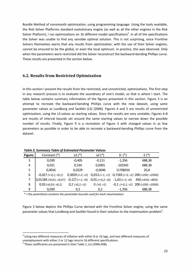
In this section I present the results from the restricted, and unrestricted, optimizations. The first step

in any research process is to evaluate the soundness of one’s model, so that is where I start. The

table below contains summary information of the figures presented in this section. Figure 3 is an

attempt to recreate the backward-bending Phillips curve with the new dataset, using same

parameter values as Lundborg and Sacklén (LS) (2006). Figures 4 and 5 are results of unrestricted

optimization, using the LS-values as starting values. Since the results are very unstable, Figures 6-8

are results of interval bounds set around the same starting values to narrow down the possible

number of results. Finally, Figure 9 is a recreation of Figure 3 with changed values in as few

parameters as possible in order to be able to recreate a backward-bending Phillips curve from the

dataset.

Figure 3 below depicts the Phillips Curve derived with the Frontline Solver engine, using the same

parameter values that Lundborg and Sacklén found in their solution to the maximization problem5.

4 Using two different measures of inflation with either 8 or 16 lags, and two different measures of

unemployment with either 2 or 12 lags returns 16 different specifications. 5 These coefficients are presented in their Table 1, (v) (2006:408).

Table 2. Summary Table of Estimated Parameter Values

Figure: Constant (*) a1 (*) a2 (*) D (*) E (*)

3 0,039 -0,405 -0,111 -1,356 688,38

4 0,021 0,534 0,0301 -102341 688,38

5 0,0016 0,0229 -0,0046 11706016 20,8

6 -0,027 (>-0,1; <0,1) 0,3659 (>-2; <2) -0,013 (>-1; <1) -0,7183 (>-3; <2) 200 (>200; <2000)

7 0,01184 (>0,01; <0,07) -0,127 (>-1; <0) -0,01 (>-0,2; <0) -1,63 (>-2; <0) 450 (>450; <800)

8 0,03 (>0,03; <0,1) 0,2 (>0,2; <2) 0 (>0; <1) -0,1 (>-0,1; <2) 200 (>200; <2000)

9 0,039 0,2 0,2 -1,356 688,38

* = the parenthesis contains the parameter bounds used for each maximization

24

In the figure above, the curve is derived from the model specification using only open unemployment

with two lags and domestic price inflation with 16 lags. When recreating the curve above with the

same parameter values but different lag structures the same picture emerges, albeit with small

differences. But the differences are too small to make notable changes in optimization results

presented below, so the lag structures used above are also used throughout the remainder of this

section. As can be seen from Figure 3, the result is in no way encouraging with regards to the ADP-

model. But the data is different from the data used by Lundborg and Sacklén, so it is in no way sure

that their parameter values are near the correct values.

The first maximizations were done, using as starting values of the parameters the values estimated

by Lundborg and Sacklén (see footnote 5), with no constraints on the parameters. This is the best

test of the model, but also the test with most pitfalls. Since there are no constraints, the Solver

engine may encounter many solutions that are only local, or just look like local maximizations. Hence,

using an engine that is not fully equipped to handle such problems, multiple maximizations with the

exact same input may yield totally different output. As it turns out, the results were very volatile.

Some of these results are presented in Figures 4 and 5 below.

25

The cause of the slope of the curve in Figure 4 above is a very large negative value of the parameter

D and a positive total value of the parameters for unemployment. However, in another optimization

with the same starting values, the following solution emerged:

In this case, the result characterizing the traditional long run Phillips curve was an effect of the

opposite of the case in Figure 4, namely a very large positive value of D. But soon a pattern emerged

in where the results were very sensitive to different maximizations, and to the choice of starting

values. A change in those values generated curves with totally different values and interpretations.

But as can be seen from Figures 4 and 5 above, the results differs a lot even with the same starting

values. The only thing in common that Figure 4 and 5 share is the positive total value of the

parameters for unemployment. Nevertheless, in most cases, the Solver engine could not even find

any solution, leaving the starting values to be the optimal solution.

Interpreting the above results, it is very clear that any unconstrained optimization would inevitably

fail. Therefore, the next step is to perform the same optimization but with constraints on the

parameter values. The restrictions are set as to let the values vary around the coefficient values

found by Lundborg and Sacklén (2006), with large intervals. This is necessarily not the best way to

continue the analysis. After all, the parameter values estimated by the previous research have varied

a lot. While both Lundborg and Sacklén (2006) and Akerlof et al. (2000) found high values of the

coefficient E, Dickens (2001) and Maugeri (2010) did not. Other parameters have varied across the

mentioned research as well, creating the different results from the studies using the ADP-model

presented above. But there are no other way to selecting the initial values, and choosing the initial

values based on previous research on the same country used in this essay is as good as it can get.

The results from this constrained optimization are presented below. In the first figure, Figure 6, the

only parameter that hit the bound was E, that hit the lower bound of 200. We can see that the

characteristic backward-bending curve is derived, but with negative unemployment numbers.

Omitting the lower bound for E creates the traditional short-run Phillips relation, but still with

negative unemployment numbers.

26

As described above, with the bounds used so far only the parameter E hit a lower bound, with a

desire to go so low that the backward-bending character of the curve vanishes to a convex relation

similar to that of the short-run Phillips curve. Since no one of the other parameters hit their bound, it

is motivated to narrow the intervals in order to help the Solver engine to find a solution within the

range that is interesting. Thai is, to narrow down the possible number of solutions and see whether

the results turn out favorable.

The result turns out to be very similar to Figure 3. This is no coincident since the only difference lies

in the smaller bounds used in the construction of Figure 7, which are in a small interval around the

values in Figure 3.

27

To summarize all the optimization up to this point, it is clear that with no constraints at all it seems to

be impossible to obtain a stable solution that resembles the backward-bending Phillips curve. But

with too much restrictions the solutions inevitably narrow down to Figure 3 which is not the result

we expect to find. From the results in Figures 3 and 7, the conclusion is that either the ADF-model is

wrong or the parameter values used to obtain these figures are wrong. Alternatively, the statistical

program used is not strong enough to generate a global maximum.

To follow up on the second conclusion and to explore the possibilities contained in Figure 6, the

following part of this chapter tries to recreate the hypothetical Phillips curve in Figure 1. This is done

by exploring the necessary restrictions that must be imposed from the original settings in Figure 6.

Unfortunately, this could turn out to be a futile attempt giving misleading results as the result in

Figure 6 was not stable at all. But all is not lost either, since repeated optimizations generated several

curves similar to Figure 6, so there seems to be a bias towards a curve like the one in Figure 6.

It turns out that, in order to recreate a curve similar to the one in Figure 1, it is necessary to impose a

lot of extra restrictions. In Figure 8 below, the following restrictions has been forced to the model in

addition to the more lax restrictions in Figure 6; D > -0,1, d > 0,03, > 0,2. In Figure 8, for the first

time, a curve similar to the results of Lundborg and Sacklén has been created. However, all the lower

bounds, mentioned above, were actively enforced.

But which of the parameters (D, E, d and ) has the greatest impact on the relation between

inflation and unemployment? With the exception of Figures 4 and 5, in most of the optimizations the

values of D have been in low absolute numbers around zero. A change in D in Figure 8 does only alter

the curvature, and not the position of the curve on the axis. A change in E does changes the curve in

major ways. A high value of E yield curves as in Figure 1 while low values of E generate curves like the

curve in Figure 4. But E, like D, does not change the position of the curve, just its slope. What does

changes the position of the curve is the constant, d, and the total coefficient value of unemployment.

But while the constant only changes the curves position on the axis, it does not change its slope. On

28

the other hand, changes in affects both the curves position on the axis and its slope. For example,

using the same parameter values as Lundborg and Sacklén (Figure 3) but changing from -0,516 to

0,4 generates the curve depicted in Figure 9 below.

As can be seen, the simple change in the total coefficient value of unemployment from a negative

value to positive value creates the same kind of Phillips relation that both Akerlof et al. (2000) and

Lundborg and Sacklén (2006) obtains. From this figure, we can easily derive the LSUR- and LSURI-

levels by looking at the lowest level of unemployment and its associated level of inflation. However,

the question on whether the counterintuitive relation between inflation and unemployment implied

by the positive coefficient value are plausible and whether the imposed restrictions are realistic

remains.

29

7. Conclusion

This essay has attempted to shed some new light on the relationship between inflation and

unemployment in Sweden, by the use of more recent data now available. Unfortunately, the

statistical software used in this essay fails to provide any concluding remarks to whether or not a

long, sustained, period of low inflation and inflation expectations alter the backward-bending shape

of the long-run Phillips curve as derived by Lundborg and Sacklén (2006). But a simple analysis can be

easily made. In order to create the backward-bending Phillips curve in Figure 9 the total value of the

coefficients for unemployment expectations, , needs to be 0,4. But is this realistic? This implies a

positive relationship between inflation and unemployment, so when inflation increases so does

unemployment. This is counterintuitive and goes against both economic theory as well as the ADP-

model. The correlation between the expected unemployment and inflation is -0.47, indicating that

there is a strong negative relationship between the variables. So it seems that the analyses of the

coefficients value implied by Figures 8 and 9 are highly unrealistic. Therefore, the question on

whether the introduction of an inflation targeting regime affects the LSURI remains partly

unanswered. In this case, the most likely reason for the unsuccessful results is that there is a need for

a better program for maximization.

The essay also summarizes the research made with the ADP-type of model, and the criticism it has

raised. Even though there is research evidence of a negative relationship between inflation and

unemployment in the long run, it is hard to draw any final conclusions. This is especially true when it

comes to the backward-bending Phillips curve proposed by Akerlof, Dickens and Perry. The more in

depth studies outside of North America seems to support this view. But these are few, and the

results from the Italian study propose very unlikely estimates of the Phillips curve.

Regarding the criticism of the ADP-model, it merits pointing out some of the more important notes

that is worth a second thought. When it comes to the use of data on inflation expectations, Bryan

and Palmqvist has provided a simple analysis to evaluate the model. Their analysis provides some

interesting results. Most notably, they find that expectation errors do not vary with the rate of

inflation. Furthermore, they attribute the stable inflation expectations in Sweden to a focal point

created when the Swedish central bank adopted its inflation target.

Their results are very interesting and worthy of consideration. However, this type of analysis ignores

the possible backward looking component of expectations. When looking at their Table 1, a pattern

emerges in where a period of high average inflation followed by a period of low inflation results in a

positive expectation error and vice versa. In fact, since in equation 14 above, represents the

effects of past inflation measured as a weighted moving average, on the likelihood that people act

rationally toward inflation, the backward looking component that is missing in the analyses of Bryan

and Palmqvist is embedded in the ADP-model. Another interesting observation is that even though

inflation expectations seem to be anchored around a focal point, this could be a result of a framing

effect that is not apparent when setting prices and wages. When people are asked explicitly of what

they expect the inflation rate to be 12 month ahead, it is likely that they formulate their answer in

relation to what they know. They may have little knowledge of other mechanisms that affect

inflation, but if they believe in the central bank’s commitment to the inflation target, they have no

reason not to expect that inflation target to be the true inflation rate in 12 month time. This is

30

apparent in Table 1, where the average expected inflation rate in Sweden has been 2,04 per cent the

last decade. However, in price and wage talks, inflation is most likely not a central but only a

peripheral question. For example, Davis, Haltiwanger and Schuh find that the typical firm annually

experiences demand shocks affecting the firm size up or down by 10 per cent. A firm who fails to

adjust its capacity to these shocks would face losses of around 10 per cent of its profit (in Akerlof et

al. 2000:15). So when it comes to wage and price settings, not only is inflation not the explicit

question but there are most likely other more pressing matters to discuss.

Concerning the implications of the ADP-model, Blinder (2000) is among those that argue that not

only high inflation but also the passage of time do contain the possibility of dissolving money illusion.

This implies that people do learn from their mistakes and with time do start to include low levels of

inflation in their mental accounts. Even though these views may not be mutually exclusive, the

implication for the ADP-model is huge. If people, in time, learn from their mistakes, there is no

reason to believe in the backwards-bending Phillips curve. It is compelling to think that we do learn

from our mistakes and that we get more rational by age. While I believe that there is no good reason

to believe that we never learn from our mistakes, it may be an artifact of traditional thinking to

believe that we always, in all situations, do. If the individual costs are so low that they are almost

negligible, while at the same time it is considerably easier and more natural for individuals to think in

nominal terms (Shafir et al. 1997), there is in fact no good reason to believe that we always learn

from these mistakes.

One of the more relevant debates that the ADP-model raises concerns the policy implications derived

from the model. Akerlof et al. argues that an inflation target that is set to low, like the common

target of two per cent, will create unnecessary high unemployment. Given the possible tradeoff

between inflation and unemployment in the ADP-model, central banks have now another reason

why to fight high inflation. The raw data from Sweden show that the average inflation rate since the

introduction of the inflation target has been well below two per cent. This shows that the inflation

target has been successful, but has generated an inflation level that is too low to be the LSURI level.

On the other hand, employment in Sweden do has increased from the record low in the early 1990s.

There are other pitfalls with near zero inflation. Monetary policies risk of becoming less effective if

the nominal interest rates hit the zero level. This is detrimental to investments as it may yield

positive real rates. Furthermore, with little or no inflation in an economic downturn downward wage

rigidities may change from being an academic issue to a real problem. Even though high inflation is

costly to growth, there is an ongoing debate on the growth effects of zero inflation. So although the

negative effects of to low inflation implied by the ADP-model is debated, there are other

considerations as well against to low inflation that should be weighed against the costs of inflation

when formulating monetary policies.

31

8. Appendix

Data sources

CPI (Consumer Price Index): 1979M01-2009M12 from Statistics Sweden. The quarterly data are

calculated as arithmetic averages of the monthly data.

IMPI (Import Price Index): 1979Q3-2009Q4 from Statistics Sweden. This is a price index of both

intermediate and consumer goods imported to Sweden. The quarterly data are arithmetic averages

of the monthly data.

GDP (Gross Domestic Product): 1979-2009 in current prices, from Statistics Sweden. Quarterly figures

are equal to their yearly values.

Import Value: 1979M01-2009M12 from Statistics Sweden. The yearly data are calculated as

arithmetic averages of the monthly figures. The quarterly data of the import shares of GDP are the

same as the yearly figures.

Survey data on expected inflation: 1979Q3-2009Q4 from the National Institute of Economic

Research. Quarterly data on households expectations on one year ahead CPI, collected every quarter.

Open unemployment: 1979Q3-2009Q4 from Statistics Sweden, Old Swedish Definition (Labor Force

Surveys). Seasonally adjusted data on open unemployment as a share of the labor force (aged 16-64).

Total unemployment: 1979Q3-2006Q4 from Statistics Sweden, Old Swedish Definition (Labor Force

Surveys). Seasonally adjusted data on open unemployment plus workers in active, business cycle

related, labor market programs6 (aged 16-64).

Dummy Variables

D1=1 for 1979:3-1980:1, zero otherwise

D2=1 for 1980:2-1981:3, zero otherwise

D3=1 for 1981:4-1983:3, zero otherwise

D4=1 for 1986:1-1986:4, zero otherwise

D5=1 for 1990:1-1991:2, zero otherwise

D6=1 for 1995:3-1996:2, zero otherwise

D7=1 for 2008:1-2008:3, zero otherwise

6 The data of workers in active labor market programs, as a share of total unemployment, comes from the

Swedish Public Employment Service.

32

9. References

Akerlof, George A.; Dickens, William T.; Fortin, Pierre; Perry, George L. “Inflation and

Unemployment in the U.S. and Canada: A Common Framework”, Economics Department, Université

du Québec à Montréal, Working Paper No. 20-16, July 2002.

Akerlof, George A.; Dickens, William T.; Perry, George L. “The Macroeconomics of Low Inflation”,

Brookings Papers on Economic Activity, 1:1996.

Akerlof, George A.; Dickens, William T.; Perry, George L. 2000. “Near-Rational Wage and Price

Setting and the Long-Run Phillips Curve”, Brookings Papers on Economic Activity, 1:2000.

Apergis, Nicholas; Miller, Stephen M.; Panethimitakis, Alexandros; Vamvakidis, Athanassios. 2005.

“Inflation Targeting and Output Growth: Evidence from Aggregate European Data”, University of

Connecticut, Department of Economics Working Paper Series, Working Paper 2005-06, March 2005.

Behr, Andreas; Pötter, Ulrich. 2009. “Downward Wage Rigidity in Europe: A New Flexible Parametric

Approach and Empirical Results”, German Economic Review 11(2): 169-187.

Billi, Roberto M.; Kahn, George A. 2008. “What Is the Optimal Inflation Rate?” Federal Reserve Bank

of Kansas City.

Blanchard, Olivier; DellÁriccia, Giovanni; Mauro, Paolo. 2010. ”Rethinking Macroeconomic Policy”,

IMF STAFF POSITION NOTE, February 12, 2010, SPN/10/03.

Blinder, A.S. 2000 .Comment on Akerlof, Dickens and Perry, .”Near- Rational Wage and Price Setting and the Long-Run Phillips Curve.”, Brookings Papers on Economic Activity No. 1, pp. 50-55. Bryan, Michael F.; Palmqvist, Stefan. 2005. ”Testing Near-rationality using Detailed Survey Data”,

Sveriges Riksbank, Working Paper Series. 183, April 2005.

Camba-Méndez, Gonzalo; García, Juan Àngel; Palenzuela, Diego Rodríguez. 2003. “Relevant

Economic Issues Concerning the Optimal Rate of Inflation”, European Central Bank, Working Paper

No. 278, September 2003.

Dickens, William T. 2001. Comment on Wyplosz, Charles. ”Do Wo Know How Low Inflation Should

Be?”, The Brookings Institution.

Fisher, Irving. 1928. “The Money Illusion”, Adelphi Company.

Friedman, Milton. 1968. “The Role of Monetary Policy”, The American Economic Review, Vol. 58, No.

1 (Mars 1968), pp. 1-17.

Fontana, Guiseppe, Palacio-Vera, Alfonso. 2007. ”ARE LONG-RUN PRICE STABILITY AND SHORT-RUN

OUTPUT STABILIZATION ALL THAT MONETARY POLICY CAN AIM FOR?”, Metroeconomica 58:2 (2007),

pp. 269-298.

Gordon, Robert J. 1996. Comment on Akerlof, Dickens and Perry, .”The Macroeconomics of Low

Inflation”, Brookings Papers on Economic Activity ,Vol. 1996, No. 1 (1996), pp. 60-66.

33

Gottschalk, Jan; Fritsche, Ulrich. 2005. “The New Keynesian Model and the long-run vertical Phillips

Curve: Does it hold for Germany?”, DIW Berlin, German Institute for Economic Research, Discussion

Papers 521.

Hogan, Seamus. 1997. ”What Does Downward Nominal-Wage Rigidity Imply for monetary Policy?”,

Bank of Canada, Working Paper 97-13.

Kahneman, Daniel; Tversky, Amos. 1979. “Prospect Theory: An Analysis of Decision under Risk”,

Econometrica, Vol. 47, No. 2 (Mars, 1979), pp. 263-292.

Keynes, John Maynard. 1936. “The General Theory of Employment, Interest and Money”, Macmillan

Cambridge University Press, for the Royal Economic Society.

Lebow, David E.; Saks, Raven E.; Wilson, Beth Anne. 1999. “Downward Nominal Wage Rigidity:

Evidence from the Employment Cost Index”, Board of Governors of the Federal Reserve System, July.

Lipsey, Richard G. 1960. “The Relation between Unemployment and the Rate of Change of Money

Wage Rates in the United Kingdom, 1861-1957: A Further Analysis”, Economica, New Series, Vol.27,

No. 105 (Feb., 1960), pp. 1-31.

Lundborg, Per; Sacklén; Hans. 2006. ”Low-inflation Targeting and Long-run Unemployment”,

Scandinavian Journal of Economics, 108(3), 397-418, 2006.

Lundborg, Per; Sacklén; Hans. 2003. ”Low-inflation Targeting and Unemployment Persistence”, FIEF

Working Paper Series 2003, No. 188, May 7, 2003.

McLaughlin, Kenneth J. 2000. ”ASYMMETRIC WAGE CHANGES AND DOWNWARD NOMINAL WAGE

RIGIDITY”, Hunter College and the Graduate Center, City University of New York, October 2000.

Maugeri, Novella. 2010. “Macroeconomic Implications of Near Rational Behavior: an Application to

the Italian Phillips Curve”, Università Defli Studi di Siena, Quaderni del dipartimento di economica

politica, n. 587, Marzo 2010.

Musy, Olivier; Pommier, Sébastien. 2007. “Inflation expectations and the structure of the New-

Keynesian Phillips Curve”. Applied Economics Letters, 2007, 14, 679-683.

Nisbett, Richard; Ross, Lee. 1980. “Human Inference. Strategies and Shortcomings of Social

Judgment.” Prentice-Hall, Englewood Cloffs, N.J., 1980. xvi, pp. 334.

Phillips, A. W. 1958. “The Relation between Unemployment and the Rate of Change of Money Wage

Rates in the United Kingdom, 1861-1957”, Economica, New Series, Vol. 25, No. 100 (Nov., 1958), pp.

283-299.

Romer, David; Romer, Christina. 2002. “The Evolution of Economic Understanding and Postwar

Stabilization Policy,” in Rethinking Stabilization Policy, Federal Reserve Bank of Kansas City.

Shafir, Eldar; Diamond, Peter; Tversky, Amos. 1997. ”Money Illusion”, The Quarterly Journal of

Economics, Vol. 112, No. 2, May, 1997, pp. 341-374.

34

Svensson, Lars E. O. 2001. Comment on Wyplosz, Charles. ”Do Wo Know How Low Inflation Should

Be?” Institute for International Economic Studies, Stockholm University; CEPR and NBER. April 2001.

Sørensen, Peter Birch; Whitta-Jacobsen, Hans Jørgen. 2010. ”Introducing Advanced

Macroeconomics. Growth and business cycles”. McGraw Hill, Second Edition.

Tobin, James. 1972. “Inflation and Unemployment”, The American Economic Review, Vol. 62, No. 1/2

(Mars 1, 1972), pp. 1-18.