MONEY SUPPLY, INFLATION AND EXCHANGE RATE MOVEMENT: … SUPPLY... · among money supply, inflation...

MONEY SUPPLY, INFLATION AND EXCHANGE RATE MOVEMENT: THE CASE OF CAMBODIA

BY BAYESIAN VAR APPROACH

Monorith Sean*

Pathairat Pastpipatkul*

Petchaluck Boonyakunakorn*

*Chiang Mai University, Thailand

http://doi.org/10.31039/jomeino.2019.3.1.5

Abstract

This research paper aims to investigate the relationship among money supply, inflation and exchange rate in Cambodia by using Bayesian Vector Autoregressive (B-VAR) approach. This study employs the monthly data in the period of October-2009 and April-2018. This research paper applies the Money-in-Utility Function (MIU) that describes the relationship between money growth and price level. Moreover, this paper also employs the Purchasing Power Parity (PPP) which shows the relationship between exchange rate and inflation. The empirical results reveal that money supply in Cambodia, depends on its previous variable. Moreover, money supply also induces the depreciation of exchange rate of Khmer Riel against US Dollar and leads to increase in inflation. Money supply induces 8% of shock to exchange rate and 0.13% to inflation based on variance decomposition while exchange rate can cause 0.024% to inflation in Cambodia. The relative low shocks from money supply to inflation and exchange rate results in supplying money with cautious manner from National Bank of Cambodia. The empirical results are found to be consistent with the theories and some empirical studied of this related fields. Keywords: Money-in-Utility(MIU), Bayesian VAR, Purchasing Power Parity(PPP), Money Supply, Inflation, Exchange Rate, Cambodia.

Received 21 November 2018

Revised 28 December 2018

Accepted 31 December 2018

Corresponding author: [email protected]

http://doi.org/10.31039/jomeino.2019.3.1.5

mailto:[email protected]

Monorith Sea M., Pastpipatku P., Boonyakunakorn P. / Journal of Management, Economics, and Industrial Organization, Vol.3 No.1, 2019, pp.63-81.

64

1. Introduction

Stability of Exchange rate and inflation rate are beheld as the objective of monetary policy which is necessary to achieve of every country. To ensure the price stability, central bank, takes an essential role in conducting monetary policy through monetary tools namely discount rate, reserve requirement ratio and operation market. These three important tools are effectively implemented to manage the money supply in the circulation to enhance the stability of price. Based on theoretical framework, an injecting too much money into the circulation leads to an increase in inflation. The inflation could also influence on exchange rate as the depreciation of value of domestic currency against other currencies.

National Bank of Cambodia (NBC) conducts monetary policy with care in the context of high dollarized economy to ensure price stability and to promote economic growth. Precisely, the broad money (M2) grew by 24% as in 2017 higher than 2016 which was 18%. Inflation rate was maintained relatively low for the last few years at nearly 2.9% (NBC, 2017). The exchange rate of Riel against US Dollar was maintained broadly stable at an average 4,050 Riel per USD. NBC has maintained a stable exchange rate through the intervention in foreign exchange market in very cautious manner to supply Riel in accordance with prevailing market mechanism and economic conditions.

Therefore, this study aims to investigate the movement of money supply, inflation and exchange rate in Cambodia by employing Bayesian Vector Autoregressive (B-VAR). This research could capture the relationship among variables and show the impulse response functions due to the endogenous shocks. Moreover, it also illustrates the variance decomposition which could present the effects among variables.

2. Literature Review

2.1.Theoretical Framework

The theory of money is initially explained by the Quantity Theory of Money (QTM). The concept of QTM is explained by the equation of exchange which states that the movement of price level results solely from changes in the quantity of money. However, this theory does not capture clearly about money supply and price level mathematically. In order to insert mathematical theoretical framework, this paper shows the micro-macroeconomic foundation of the Money-in-Utility function which illustrates the super-neutrality of money. Money growth only induces inflation in the steady states. In other words, inflation will increase with the same proportion as money growth (Lewis and Mizen, 2000).

The model of money utility function is developed by Sidrauski (1967) who introduced money into the classical growth model.

Suppose that utility function of representative household is given by: 𝑊𝑊 = 𝐸𝐸𝑡𝑡 ∑ 𝛽𝛽𝑡𝑡∞

𝑡𝑡=0 𝑢𝑢(𝑐𝑐𝑡𝑡 ,𝑚𝑚𝑡𝑡), 0 < 𝛽𝛽 < 1


65

Where

• 𝑐𝑐𝑡𝑡 is per capita consumption at time t. • 𝑚𝑚𝑡𝑡 is real money balance, 𝑚𝑚𝑡𝑡 = 𝑀𝑀𝑡𝑡

𝑃𝑃𝑡𝑡𝑁𝑁𝑡𝑡 , 𝑀𝑀𝑡𝑡 normal money balance and 𝑁𝑁𝑡𝑡

is population. • 𝛽𝛽 is discount factor

The utility function is assumed to be increasing in both arguments and its function form is:

𝑢𝑢(𝑐𝑐𝑡𝑡,𝑚𝑚𝑡𝑡) = �𝑐𝑐𝑡𝑡𝑚𝑚𝑡𝑡𝜎𝜎

1−𝜑𝜑�1−𝜑𝜑

, 𝜎𝜎 𝑎𝑎𝑎𝑎𝑎𝑎 𝜑𝜑 > 0

And household has budget constraint

𝑦𝑦𝑡𝑡 + 𝜏𝜏𝑡𝑡 + (1 − 𝛿𝛿)𝑘𝑘𝑡𝑡−1 + 𝑚𝑚𝑡𝑡−1

1 + 𝜋𝜋𝑡𝑡= 𝑐𝑐𝑡𝑡 + 𝑘𝑘𝑡𝑡 + 𝑚𝑚𝑡𝑡

Where

• 𝑦𝑦𝑡𝑡 is output per capita

• 𝜏𝜏𝑡𝑡 is government transfer

• 𝑘𝑘𝑡𝑡−1 is capital per capita at time t-1

• 𝑚𝑚𝑡𝑡−1 is real money balance at time t-1

• 1 + 𝜋𝜋𝑡𝑡 is inflation

Let suppose that 𝑦𝑦𝑡𝑡 = 𝑓𝑓(𝑘𝑘𝑡𝑡−1) = 𝑘𝑘𝑡𝑡−1𝛼𝛼 is production function represents output per

capita. Hence, household maximize her utility subject to budget constraint through

Lagrangian function:

ℒ = 𝐸𝐸𝑡𝑡 ��𝛽𝛽𝑡𝑡 �(𝑐𝑐𝑡𝑡𝑚𝑚𝑡𝑡

𝜎𝜎)1−𝜑𝜑

1 − 𝜑𝜑�

∞

𝑡𝑡=0

+ �𝛽𝛽𝑡𝑡𝜆𝜆𝑡𝑡 �𝑘𝑘𝑡𝑡−1𝛼𝛼 + 𝜏𝜏𝑡𝑡 + (1 − 𝛿𝛿)𝑘𝑘𝑡𝑡−1 +𝑚𝑚𝑡𝑡−1

1 + 𝜋𝜋𝑡𝑡− 𝑐𝑐𝑡𝑡 − 𝑘𝑘𝑡𝑡 − 𝑚𝑚𝑡𝑡 �

∞

𝑡𝑡=0

�

The First-Order Conditions (FOCs) are:

𝜕𝜕ℒ𝜕𝜕𝑐𝑐𝑡𝑡

= 𝑐𝑐𝑡𝑡−𝜑𝜑 (𝑚𝑚𝑡𝑡

𝜎𝜎)1−𝜑𝜑 − 𝜆𝜆𝑡𝑡 = 0

𝜆𝜆𝑡𝑡 = 𝑐𝑐𝑡𝑡−𝜑𝜑 (𝑚𝑚𝑡𝑡

𝜎𝜎)1−𝜑𝜑 (1)

𝜕𝜕ℒ𝜕𝜕𝑚𝑚𝑡𝑡

= 𝜎𝜎𝑐𝑐𝑡𝑡1−𝜑𝜑(𝑚𝑚𝑡𝑡

𝜎𝜎)𝜎𝜎(1−𝜑𝜑)−1 + 𝛽𝛽𝜆𝜆𝑡𝑡+1

1 + 𝜋𝜋𝑡𝑡+1− 𝜆𝜆𝑡𝑡 = 0


66

𝜆𝜆𝑡𝑡 = 𝜎𝜎𝑐𝑐𝑡𝑡1−𝜑𝜑(𝑚𝑚𝑡𝑡

𝜎𝜎)1−𝜑𝜑 + 𝛽𝛽 𝜆𝜆𝑡𝑡+11+𝜋𝜋𝑡𝑡+1

(2)

𝜕𝜕ℒ𝜕𝜕𝑘𝑘𝑡𝑡

= 𝛼𝛼𝛽𝛽𝑡𝑡+1𝜆𝜆𝑡𝑡+1𝑘𝑘𝑡𝑡𝛼𝛼−1 + 𝛽𝛽𝑡𝑡+1𝜆𝜆𝑡𝑡+1(1 − 𝛿𝛿) − 𝜆𝜆𝑡𝑡𝛽𝛽𝑡𝑡 = 0

𝜆𝜆𝑡𝑡 = 𝛽𝛽𝐸𝐸𝑡𝑡[𝜆𝜆𝑡𝑡+1 (𝛼𝛼𝑘𝑘𝑡𝑡𝛼𝛼−1 + (1 − 𝛿𝛿))] (3)

If we substitute (1) into (2), we get

𝑐𝑐𝑡𝑡−𝜑𝜑 (𝑚𝑚𝑡𝑡

𝜎𝜎)1−𝜑𝜑 = 𝜎𝜎𝑐𝑐𝑡𝑡1−𝜑𝜑(𝑚𝑚𝑡𝑡

𝜎𝜎)𝜎𝜎(1−𝜑𝜑)−1 + 𝛽𝛽 𝑐𝑐𝑡𝑡+1−𝜑𝜑 (𝑚𝑚𝑡𝑡+1

𝜎𝜎 )1−𝜑𝜑

1+𝜋𝜋𝑡𝑡+1 (4)

(4) states that the marginal benefit of adding to money holding at time t must equal to the

marginal utility of consumption.

If we plug (1) into (3) we get,


𝜎𝜎)1−𝜑𝜑 = 𝛽𝛽 𝑐𝑐𝑡𝑡+1−𝜑𝜑 (𝑚𝑚𝑡𝑡+1

𝜎𝜎 )1−𝜑𝜑[𝛼𝛼𝑘𝑘𝑡𝑡𝛼𝛼−1 + (1 − 𝛿𝛿)] (5)

(5) states that the marginal return for holding additional capital must equal marginal utility

of consumption.

If we recall the real money balance for household holding,

𝑀𝑀𝑡𝑡𝑃𝑃𝑡𝑡𝑁𝑁𝑡𝑡

= 𝑀𝑀𝑡𝑡−1𝑃𝑃𝑡𝑡𝑁𝑁𝑡𝑡

+ 𝜏𝜏𝑡𝑡 (6)

The above equation illustrates that money that household holds is the previous money at

time t-1 and the transfer from government.

(6) could be written as:


= 𝑀𝑀𝑡𝑡−1𝑃𝑃𝑡𝑡−1𝑃𝑃𝑡𝑡𝑁𝑁𝑡𝑡

𝑃𝑃𝑡𝑡−1 + 𝜏𝜏𝑡𝑡 (7)

Moreover,

𝜏𝜏𝑡𝑡 = Δ𝑀𝑀𝑡𝑡𝑃𝑃𝑡𝑡𝑁𝑁𝑡𝑡

= 𝑀𝑀𝑡𝑡𝑃𝑃𝑡𝑡𝑁𝑁𝑡𝑡

− 𝑀𝑀𝑡𝑡−1𝑃𝑃𝑡𝑡𝑁𝑁𝑡𝑡

(8)

Or

𝜏𝜏𝑡𝑡 = Δ𝑀𝑀𝑡𝑡𝑃𝑃𝑡𝑡𝑁𝑁𝑡𝑡

= 𝑀𝑀𝑡𝑡𝑃𝑃𝑡𝑡𝑁𝑁𝑡𝑡

− 𝑀𝑀𝑡𝑡−1𝑃𝑃𝑡𝑡−1𝑃𝑃𝑡𝑡𝑁𝑁𝑡𝑡

𝑃𝑃𝑡𝑡−1 (9)

But

𝑀𝑀𝑡𝑡 = (1 + 𝑔𝑔𝑡𝑡)𝑀𝑀𝑡𝑡−1 is money growth rate


67

The (9) could be written as:

𝜏𝜏𝑡𝑡 = (1+𝑔𝑔𝑡𝑡)𝑀𝑀𝑡𝑡−1𝑃𝑃𝑡𝑡−1𝑃𝑃𝑡𝑡𝑁𝑁𝑡𝑡

𝑃𝑃𝑡𝑡−1 −𝑀𝑀𝑡𝑡−1

𝑃𝑃𝑡𝑡−1𝑃𝑃𝑡𝑡𝑁𝑁𝑡𝑡𝑃𝑃𝑡𝑡−1 (10)

Then,

𝜏𝜏𝑡𝑡 = (1 + 𝑔𝑔𝑡𝑡)𝑚𝑚𝑡𝑡−1𝑃𝑃𝑡𝑡−1

𝑃𝑃𝑡𝑡−𝑚𝑚𝑡𝑡−1𝑃𝑃𝑡𝑡−1

𝑃𝑃𝑡𝑡

Hence,

𝜏𝜏𝑡𝑡 = 𝑔𝑔𝑡𝑡𝑚𝑚𝑡𝑡−11+𝜋𝜋𝑡𝑡

(11)

Where

• 𝑚𝑚𝑡𝑡−1 = 𝑀𝑀𝑡𝑡−1𝑃𝑃𝑡𝑡−1𝑁𝑁𝑡𝑡

and 𝑃𝑃𝑡𝑡−1𝑃𝑃𝑡𝑡

= 11+𝜋𝜋𝑡𝑡

is inflation

• 𝑁𝑁𝑡𝑡 = 𝑁𝑁𝑡𝑡−1 = ……………… Labor at all times is assumed to be fixed.

If we substitute (11) into (7) we get,


= 𝑀𝑀𝑡𝑡−1𝑃𝑃𝑡𝑡−1𝑃𝑃𝑡𝑡𝑁𝑁𝑡𝑡

𝑃𝑃𝑡𝑡−1 + 𝑔𝑔𝑡𝑡𝑚𝑚𝑡𝑡−11+𝜋𝜋𝑡𝑡

(12)

Then,

𝑚𝑚𝑡𝑡 = 𝑚𝑚𝑡𝑡−11+𝜋𝜋𝑡𝑡

+ 𝑔𝑔𝑡𝑡𝑚𝑚𝑡𝑡−11+𝜋𝜋𝑡𝑡

Or

𝑚𝑚𝑡𝑡 = (1+𝑔𝑔𝑡𝑡)𝑚𝑚𝑡𝑡−11+𝜋𝜋𝑡𝑡

(13)

In steady state, there is no time subscript. Hence (13) could be written as:

𝑚𝑚 = (1 + 𝑔𝑔)𝑚𝑚

1 + 𝜋𝜋

Hence

𝑔𝑔 = 𝜋𝜋 (14)


68

(14) implies that money growth rate equal to the price level or inflation. Hence this

confirms the increase in money growth induces the inflation.

If we recall the budget constraint,

𝑘𝑘𝑡𝑡−1𝛼𝛼 + 𝜏𝜏𝑡𝑡 + (1 − 𝛿𝛿)𝑘𝑘𝑡𝑡−1 + 𝑚𝑚𝑡𝑡−11+𝜋𝜋𝑡𝑡

− 𝑐𝑐𝑡𝑡 − 𝑘𝑘𝑡𝑡 − 𝑚𝑚𝑡𝑡 (15)

Where 𝜏𝜏𝑡𝑡 = 𝑔𝑔𝑡𝑡𝑚𝑚𝑡𝑡−11+𝜋𝜋𝑡𝑡

and 𝑚𝑚𝑡𝑡 = (1+𝑔𝑔𝑡𝑡)𝑚𝑚𝑡𝑡−11+𝜋𝜋𝑡𝑡

Then (15) could be written as:

𝑘𝑘𝑡𝑡−1𝛼𝛼 + 𝑔𝑔𝑡𝑡𝑚𝑚𝑡𝑡−1

1 + 𝜋𝜋𝑡𝑡+ (1 − 𝛿𝛿)𝑘𝑘𝑡𝑡−1 +

𝑚𝑚𝑡𝑡−1

1 + 𝜋𝜋𝑡𝑡= 𝑐𝑐𝑡𝑡 + 𝑘𝑘𝑡𝑡 +

(1 + 𝑔𝑔𝑡𝑡)𝑚𝑚𝑡𝑡−1

1 + 𝜋𝜋𝑡𝑡

Then,

𝑘𝑘𝑡𝑡−1𝛼𝛼 + (1 − 𝛿𝛿)𝑘𝑘𝑡𝑡−1 = 𝑐𝑐𝑡𝑡 + 𝑘𝑘𝑡𝑡 (16)

If we recall (5)


𝜎𝜎)1−𝜑𝜑 = 𝛽𝛽 𝑐𝑐𝑡𝑡+1−𝜑𝜑 (𝑚𝑚𝑡𝑡+1

𝜎𝜎 )1−𝜑𝜑[𝛼𝛼𝑘𝑘𝑡𝑡𝛼𝛼−1 + (1 − 𝛿𝛿)]

In steady state,

𝑐𝑐−𝜑𝜑(𝑚𝑚)𝜎𝜎(1−𝜑𝜑) = 𝛽𝛽𝑐𝑐−𝜑𝜑(𝑚𝑚)𝜎𝜎(1−𝜑𝜑)[𝛼𝛼𝑘𝑘𝛼𝛼−1 + (1 − 𝛿𝛿)]

Then,

𝛼𝛼𝑘𝑘𝛼𝛼−1 + (1 − 𝛿𝛿) = 1𝛽𝛽

Hence,

𝑘𝑘∗ = �1𝛽𝛽−1+𝛿𝛿

𝛼𝛼�1𝛼𝛼−1�

(17)

Then (16) in steady state

𝑘𝑘𝛼𝛼 + (1 − 𝛿𝛿)𝑘𝑘 = 𝑐𝑐 + 𝑘𝑘

Then

𝑐𝑐∗ = �1𝛽𝛽−1+𝛿𝛿

𝛼𝛼�𝛼𝛼𝛼𝛼−1�

− 𝛿𝛿 �1𝛽𝛽−1+𝛿𝛿

𝛼𝛼�1𝛼𝛼−1�

(18)


69

Hence,

𝑦𝑦∗ = 𝑓𝑓(𝑘𝑘) = �1𝛽𝛽−1+𝛿𝛿

𝛼𝛼�𝛼𝛼𝛼𝛼−1�

(19)

Based on Money in Utility Function, money is super-neutrality and neutrality since (17)-(19) illustrate that real variables are independent from policy variable. Moreover, an increase in money growth rate proportionally leads to increase in price level which known as inflation. Hence, this theory aims to explain a positive correlation between inflation and money supply growth.

The theory of money supply and exchange rate is explained through the monetary approach. This theory states that exchange rate is expressed through the balance of payment since it is the price of one currency in terms of another currency. The model starts with the reasonable statement that as the exchange rate is the relative price of foreign and domestic money, it should be determined by the relative supply and demand for this money (Frankel and Rose, 1994). With monetary approach therefore, it is important to emphasize the role of demand and supply of money in determining the exchange rates.

The theory of exchange rate and inflation is captured through Purchasing Power Parity (PPP). This theory attempts to quantify inflation and exchange rate relationship by insisting that change in exchange rate is caused by inflation rate differentials (Ndung'u, 1997). He indicated that exchange rate must change to adapt the change in the prices of goods in the two countries. The PPP in simplest form echoed that in the long run, change in exchange rate among countries will tend to reflect change in relative price.

2.2.Empirical Studies

Many empirical analyses have studied in this related topic. Precisely, (Vogel, 1974) investigated the impact of change of money growth on the general price in Latin America. He pointed out that an increase in money growth rate leads to increase in inflation as the same rate. (Abdullah & Yusop, 1996) employed quarterly data in the period of 1970-1992 to analyze the causality between money growth and inflation in Malaysia. He indicates that there is a unidirectional causality from money supply to inflation. (Bengali, Khan and Sadaqat, 1999) showed that an increase in money supply induces inflation rate in Pakistan. (Bafekr, 1998) investigated the most significant factors that possibly influence on inflation in Iran. He indicates that 10% increases in liquidity in the long run causes inflation to increase by 2.7% as in retail sales and 3.2% as in whole sales. Moreover, (Dawoodi, 1997) also stated that 1% increase in liquidity which is 95% as confident level could induce 1% increase in exchange rate and cause inflation to increase by 0.301%. (Levin, 1997) showed that money growth causes domestic currency to depreciate. (Kazerooni and Asghari, 2002) examined the relationship between money supply and


70

inflation in Iran. He indicates that money supply and inflation has a positive correlation. (İsfahani, 2003) concluded that an increase in money supply causes exchange rate to jump up and inflation expectation to increase where inflation is treated as normal variables in the VAR 1971-2001 of his model. (Okhiria, & Saliu, 2008) pointed that money supply and exchange rate has a great impact on inflation in Nigeria. (Simwaka, et al. 2012) indicates that money supply growth drives inflation with lags of 3 to 6 months. Moreover, he also confirmed that exchange rate is relatively more significant to induce inflation in Malawi. (Madesha et al., 2013) illustrated that there is a long run relationship between inflation rate and exchange rate in Zimbabwe. (Adeniji, 2013) demonstrated that there is a positive significant correlation among exchange rate, inflation and money supply in Nigeria by employing VECM model in the period of 1986-2012.

3. Data Description

This empirical study is conducted through monthly data in the period of October 2009-April 2018. All variables such as money supply (MS), inflation (INF) and exchange rate (ER) are mainly extracted from Economic and Monetary Statistic of National Bank of Cambodia (NBC).

4. Research Methodology

4.1. Vector Autoregressive Model (VAR)

Vector Autoregressive Model (VAR) model is developed by Christopher Sims (1980) with the aim of analyzing multivariate time series data (Christiano, 2012). The VAR(q) model can be written as:

𝑦𝑦𝑡𝑡 = 𝑐𝑐 + ∑ 𝐵𝐵𝑗𝑗𝑞𝑞𝑗𝑗=1 𝑦𝑦𝑡𝑡−𝑗𝑗 + 𝜀𝜀𝑡𝑡 (20)

In this study, there are three necessary variables to be observed, namely money supply

(MS), exchange rate (EX), and inflation rate (INF).

Where

• MS: is money supply Broad Money (M2) In Million Riel

• EX: is exchange rate of Khmer Riel against US Dollar

• INF: is inflation Consumer Price Index (CPI)

Hence, the VAR(q) could be written:


71

𝑀𝑀𝑀𝑀1,𝑡𝑡 = 𝛼𝛼1 + ∑ 𝛽𝛽1,𝑗𝑗𝑞𝑞𝑗𝑗=1 𝑀𝑀𝑀𝑀1,𝑡𝑡−𝑗𝑗 + ∑ 𝜃𝜃1,𝑗𝑗

𝑞𝑞𝑗𝑗=1 𝐸𝐸𝐸𝐸1,𝑡𝑡−𝑗𝑗 + ∑ 𝛿𝛿1,𝑗𝑗

𝑞𝑞𝑗𝑗=1 𝐼𝐼𝑁𝑁𝐼𝐼1,𝑡𝑡−𝑗𝑗 + 𝜇𝜇1𝑡𝑡 (21)

𝐸𝐸𝐸𝐸1,𝑡𝑡 = 𝛼𝛼2 + ∑ 𝛽𝛽2,𝑗𝑗𝑞𝑞𝑗𝑗=1 𝑀𝑀𝑀𝑀1,𝑡𝑡−𝑗𝑗 + ∑ 𝜃𝜃2,𝑗𝑗

𝑞𝑞𝑗𝑗=1 𝐸𝐸𝐸𝐸1,𝑡𝑡−𝑗𝑗 + ∑ 𝛿𝛿2,𝑗𝑗

𝑞𝑞𝑗𝑗=1 𝐼𝐼𝑁𝑁𝐼𝐼1,𝑡𝑡−𝑗𝑗 𝜇𝜇2𝑡𝑡 (22)

𝐼𝐼𝑁𝑁𝐼𝐼1,𝑡𝑡 = 𝛼𝛼3 + ∑ 𝛽𝛽3,𝑗𝑗𝑞𝑞𝑗𝑗=1 𝑀𝑀𝑀𝑀1,𝑡𝑡−𝑗𝑗 + ∑ 𝜃𝜃3,𝑗𝑗

𝑞𝑞𝑗𝑗=1 𝐸𝐸𝐸𝐸1,𝑡𝑡−𝑗𝑗 + ∑ 𝛿𝛿3𝑗𝑗

𝑞𝑞𝑗𝑗=1 𝐼𝐼𝑁𝑁𝐼𝐼1,𝑡𝑡−𝑗𝑗 + 𝜇𝜇3𝑡𝑡 (23)

4.2. Bayesian VAR (B-VAR)

BVAR is suggested by Litterman (1985) for econometric models and other time series techniques. According to Sims and Zha (1995), they have shown how to compute Bayesian error bands for impulse response estimated from reduced from VAR (Sims and Zha, 1998).

So, VAR equation namely, (21)-(23) could be written in a matrix form below: 𝑌𝑌 = 𝐸𝐸𝐵𝐵 + 𝐸𝐸 (24)

Where

Y is an1×1 matrix of exogenous variables,

X is an1×1 matrix of endogenous variables,

B is an 3×1matrix of coefficients

E is an1×1 matric-variate normal distribution matrix.

Canova (2007) and Geweke (2005) note a useful, alternative vectorized form of (24)

𝑦𝑦 = (𝕀𝕀𝑚𝑚 ⊗ 𝐸𝐸)𝐴𝐴 + 𝜖𝜖 (25)

Where 𝐴𝐴 = 𝑣𝑣𝑣𝑣𝑐𝑐(𝐵𝐵), vec is the Column-stacking operator , 𝑦𝑦((𝑇𝑇×𝑚𝑚)×1) = 𝑣𝑣𝑣𝑣𝑐𝑐(𝑌𝑌) is the

stacked matrix of observations, 𝜖𝜖((𝑇𝑇×𝑚𝑚)×1)~ (0, Σ⨂𝕀𝕀𝑇𝑇) is stacked vector of disturbance

terms, 𝕀𝕀𝑇𝑇 is an identity matrix of size 𝑇𝑇 × 𝑇𝑇, and ⨂ is the kronecker product.

The first B-VAR model is considered as the normal-inverse-Wishart model, where the

kernel of the joint posterior distribution could be written as:

𝑝𝑝(𝐴𝐴, Σ|𝐿𝐿,𝑦𝑦) ∝ 𝑝𝑝(𝑦𝑦|𝐿𝐿,𝐴𝐴, Σ)𝑝𝑝(𝐴𝐴, Σ) (26)

Where

𝑝𝑝(𝐴𝐴, Σ|𝐿𝐿,𝑦𝑦) is the posterior distribution

𝑝𝑝(𝑦𝑦|𝐿𝐿,𝐴𝐴, Σ) is the likelihood function which is already derived from the data set

𝑝𝑝(𝐴𝐴, Σ) is the prior distribution


72

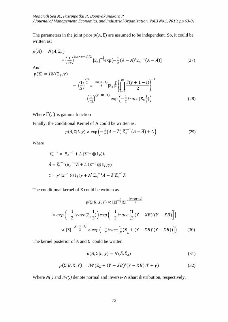
The parameters in the joint prior 𝑝𝑝(𝐴𝐴, Σ) are assumed to be independent. So, it could be written as:

𝑝𝑝(𝐴𝐴) = 𝑁𝑁(�̅�𝐴,Ξ𝐴𝐴)

= � 12𝜋𝜋�

(𝑚𝑚×𝑝𝑝+1)/2|Ξ𝐴𝐴|−

12exp [−1

2(𝐴𝐴 − �̅�𝐴)′Ξ𝐴𝐴−1(𝐴𝐴 − �̅�𝐴)] (27)

And 𝑝𝑝(Σ) = 𝐼𝐼𝑊𝑊(ΞΣ, 𝛾𝛾)

= �12�𝛾𝛾𝑚𝑚2𝜋𝜋−

𝑚𝑚(𝑚𝑚−1)4 |ΞΣ|

𝛾𝛾2 ��

Γ(𝛾𝛾+ 1− 𝑖𝑖)2

𝑚𝑚

𝑖𝑖=1�−1

. � 1|Σ|�

(𝛾𝛾−𝑚𝑚−1)exp �− 1

2𝑡𝑡𝑡𝑡𝑎𝑎𝑐𝑐𝑣𝑣(ΞΣ

1Σ)� (28)

Where Γ(. ) is gamma function

Finally, the conditional Kernel of A could be written as:

𝑝𝑝(𝐴𝐴, Σ|𝐿𝐿,𝑦𝑦) ∝ exp �− 12 �𝐴𝐴 − 𝐴𝐴��

′Σ𝐴𝐴�

−1�𝐴𝐴 − 𝐴𝐴��+ 𝐶𝐶� (29)

Where

Σ𝐴𝐴�−1 = Ξ𝐴𝐴−1 + 𝐿𝐿′(Σ−1 ⊗ 𝕝𝕝𝑇𝑇)𝐿𝐿

�̃�𝐴 = Σ𝐴𝐴�−1(Ξ𝐴𝐴−1𝐴𝐴� + 𝐿𝐿′(Σ−1 ⊗ 𝕝𝕝𝑇𝑇)𝑦𝑦)

𝐶𝐶 = 𝑦𝑦′(Σ−1 ⊗ 𝕝𝕝𝑇𝑇)𝑦𝑦 + 𝐴𝐴�′ Ξ𝐴𝐴−1�̅�𝐴 − 𝐴𝐴�′Σ𝐴𝐴�−1𝐴𝐴�

The conditional kernel of Σ could be written as

𝑝𝑝(Σ|𝐵𝐵,𝐸𝐸,𝑌𝑌) ∝ |Σ|−𝑇𝑇2|Σ|−

(𝛾𝛾−𝑚𝑚−1)2

× 𝑣𝑣𝑒𝑒𝑝𝑝 �−12𝑡𝑡𝑡𝑡𝑎𝑎𝑐𝑐𝑣𝑣(ΞΣ

1Σ

)� 𝑣𝑣𝑒𝑒𝑝𝑝 �−12𝑡𝑡𝑡𝑡𝑎𝑎𝑐𝑐𝑣𝑣 �

1Σ

(𝑌𝑌 − 𝐸𝐸𝐵𝐵)′(𝑌𝑌 − 𝐸𝐸𝐵𝐵)��

∝ |Σ|−(𝛾𝛾−𝑚𝑚−1)

2 × 𝑣𝑣𝑒𝑒𝑝𝑝 �−12𝑡𝑡𝑡𝑡𝑎𝑎𝑐𝑐𝑣𝑣 �1

Σ (ΞΣ

+ (𝑌𝑌− 𝐸𝐸𝐵𝐵)′(𝑌𝑌− 𝐸𝐸𝐵𝐵))�� (30)

The kernel posterior of A and Σ could be written:

𝑝𝑝(𝐴𝐴, Σ|𝐿𝐿,𝑦𝑦) = 𝑁𝑁(�̃�𝐴, Σ�𝐴𝐴) (31)

𝑝𝑝(Σ|𝐵𝐵,𝐸𝐸,𝑌𝑌) = 𝐼𝐼𝑊𝑊(ΞΣ + (𝑌𝑌 − 𝐸𝐸𝐵𝐵)′(𝑌𝑌 − 𝐸𝐸𝐵𝐵),𝑇𝑇 + 𝛾𝛾) (32)

Where N(.) and IW(.) denote normal and inverse-Wishart distribution, respectively.


73

5. Empirical Results

5.1.Unit Root Test

Before estimating B-VAR, there is necessary to access the unit root test. The unit root

test confirms the stationary of variables. If the data is non-stationary, it will produce the

spurious regression.

Table 1: Unit Root Test Result (ADF Test)

Variables

Level 1st difference Constant Constant and

Trend Constant Constant

and Trend MS 3.077 -0.052 -7.005* -7.980* INF -0.457 -3.181*** -8.800* -8.768* ER -3.199** -3.368*** -6.895* -6.970*

Source: Author’s own calculation Note: *, **, *** denotes significant level at 1%, 5% and 10%, respectively.

Based on table 1, it can be seen clearly that money supply is non-stationary in level I

(0). However, it confirms stationary in first difference I (1) with significant level, 1% for

both constant as well as constant and trend. Inflation is non-stationary at level for

constant. However, it is stationary in level for constant and trend with significant level,

10 %. Moreover, inflation indicates stationary in first difference. Last but not least,

exchange rate confirms stationary in level with 5% and 10% for constant and constant

and trend, respectively. Moreover, exchange rate is stationary significant level, 1% in the

first difference. To ensure the stationary process, all equations are written in first

difference since all variables confirm stationary in this level.

5.2.Lag Length Selection Criterion

Table 2: Lag Length Selection Criterion

Lag LogL LR FPE AIC SC HQ 0 -1275.487 NA 1.31e+08 27.201 27.283* 27.234* 1 -1262.461 24.942 1.20e+08* 27.116* 27.440 27.247 2 -1259.623 5.253 1.37e+08 27.247 27.815 27.476 3 -1251.562 14.407 1.40e+08 27.267 28.078 27.595

Source: Author’s own calculation *indicates lag order selected by the criterion

It is necessary to choose lag for VAR (q). The lag length selection is chosen based on the

minimum value of Akaike Information Criterion (AIC), Schwarz Information Criterion


74

(SIC) and Hannan-Quinn Information Criterion (HQ) and Final Prediction Error (FPE).

Based on table 2, lag 1 is selected due to the minimum value of AIC and FPE.

5.3.Stability of VAR

This is necessary to access the stability of VAR. If VAR confirms the stability, roots are

located in the unit circle. Based on figure 1, it is clearly seen that all roots are in the unit

circle which confirms the stability of VAR.

Figure 1: VAR Stability Source: Author’s own calculation

5.4. Estimation of Coefficients

After checking stationary, lag selection and stability of VAR, the estimation of B-VAR

with inverse-normal Wishart prior is provided with lag 1 and three necessary equations

as follow:

Table 3: B-VAR Coefficients

Variables 𝑫𝑫(𝑴𝑴𝑴𝑴) 𝑫𝑫(𝑰𝑰𝑰𝑰𝑰𝑰) 𝑫𝑫(𝑬𝑬𝑬𝑬)

𝑫𝑫(𝑴𝑴𝑴𝑴) 0.339

[ 3.528] 0.000348

[ 0.28763] 0.005

[ 1.526]

𝑫𝑫(𝑰𝑰𝑰𝑰𝑰𝑰) -86.127 [-1.019]

0.126 [ 1.193]

1.747 [ 0.540]

𝑫𝑫(𝑬𝑬𝑬𝑬)

-0.350 [-0.128]

0.000528 [ 0.154]

0.236 [ 2.264]

Constant

432.538 [ 4.738]

0.321 [ 2.80755]

-4.896 [-1.402]

Source: Author’s own calculation Note: [] denotes standard error D() represents first difference


75

There are three necessary equations to be discussed. First, there is a money supply

equation. From this equation, it can be seen clearly that the money supply at time t only

depends on its own lag t-1 with the mean (0.339) and standard error (3.528). However,

inflation and exchange rate at time t-1 display negatively on money supply at time t.

Based on money supply equation, it could be said that the amount of money supply at

time t continuously increases due to its previous amount. Based on statistical point of

view, the money supply is continuously increased due to the fact as NBC still injects more

money in the circulation.

Second equation is an inflation equation. Based on this equation, it illustrates that money

supply and exchange rate at time t-1 positively influence inflation at time t with the mean

(0.0000348) and (0.000528) and standard error (0.287) and (0.114) for money supply and

exchange rate at time t-1, respectively. According to this statistical result, it is clearly

demonstrated that an increase in money supply causes inflation rate to rise. This finding

is consistent with the theory of MIU. Moreover, it also supports (Simwaka, et al. 2012)

and (Kazerooni and Asghari, 2002) who confirmed a positive correlation between money

supply and inflation. Furthermore, a positive correlation between exchange rate and

inflation in Cambodia is also statistically confirmed. This result is found to be consistent

with the theory of PPP. Moreover, this finding also supports some empirical studies

(Madesha et al., 2013) and (Adeniji, 2013). In accordance with this statistical result, it

indicates that the depreciation of Khmer Riel against US Dollar leads to increase in

inflation due to the depreciation of Khmer Riel.

Last but not least, there is an exchange rate equation. Based on this equation, the exchange

rate at time t depends on money supply at time t-1 with the mean (0.005) and standard

error (1.52652). Inflation and exchange rate at time t-1, moreover, positively influence on

exchange rate at time t with the mean (1.747) and (0.005) and standard error (0.540) and

(1.526) for inflation and exchange rate at time t-1 respectively. Based on this statistical

finding, an increase in money supply causes exchange rate of Khmer Riel depreciates

against US Dollar.


76

5.5.Impulse Response Function

The impulse responses to the related variables presented are estimated over a period of twenty monthly horizons. The shocks increase by a value of one standard deviation and then a shock changes on variable itself and other variables.

Based on Figure 1, it is clearly seen that the shock from money supply on itself displays a decrease trend. However, response from the shock is in the positive side. The response of shock becomes stable after the fifth period.

Moreover, the shock from money supply to inflation illustrates an upward trend. The response slightly increases for the first two period and decreases after the third period. The response becomes stable after the fifth period. This shock indicates that an increase in inflation results in increasing money supply. However, due to the money supply is done with care by NBC; the inflation rate slightly decreases to in stable value as it is shown in the impulse response.

Furthermore, the shock from money supply causes exchange rate increases due to the depreciation of Khmer Riel. Based on Figure 2, it indicates that exchange rate jumps up for the first two period and reaches to the stable path after the fifth period. This confirms that the depreciation of Khmer Riel is controlled by the policy tools from NBC through stabilizing the exchange rate stability.

Figure 2: Impulse Responses Function


77

5.6.Variance Decomposition

In order to find the share of variation in a given variable caused by different shocks, the variance decomposition in B-VAR is applied. Variance decomposition, based on Table 4, takes 10 periods that help to visual the effect of related variables.

Based on the variance decomposition, money supply can cause its own shock approximately 98% both as in shot run and a long run trend. However, inflation and exchange rate display a very low percentage of shock on money supply.

Furthermore, inflation which is given in variance decomposition causes 99% to its own shocks. Money supply, moreover, causes approximately 0.13% to inflation for both short run and a long run trend. Furthermore, exchange rate causes only 0.024% to inflation. This low shocks could be explained due to the fact as NBC has achieve its goal through ensuring the price stability in terms of inflation rate and exchange rate.

Exchange rate, furthermore, responds 80% to its own shocks while money supply can cause approximately 8% to exchange rate. The related lower shock from money supply to exchange rate could be explained due to the cautious manner in supply money in a high dollarized economic context in Cambodia by NBC.

Table 4: Variance Decomposition

Source: Author’s own calculation

Per 1 2 3 4 5 6 7 8 9 10 Variance Decomposition of MS

MS 100 98.89 98.65 96.61 98.61 98.61 98.61 98.61 98.61 98.61 INF 0.00 1.090 1.327 1.360 1.364 1.365 1.365 1.365 1.365 1.365 ER 0.00 0.013 0.019 0.021 0.021 0.021 0.021 0.021 0.021 0.021

Variance Decomposition of INF MS 0.000 0.097 0.124 0.128 0.129 0.129 0.129 0.129 0.129 0.129 INF 99.99 99.88 99.85 99.84 99.84 99.84 99.84 99.84 99.84 99.84 ER 0.00 0.022 0.024 0.024 0.024 0.024 0.024 0.024 0.024 0.024

Variance Decomposition of ER MS 3.930 6.964 7.729 7.858 7.876 7.878 7.879 7.879 7.879 7.879 INF 11.40 12.01 11.92 11.91 11.90 11.90 11.90 11.90 11.90 11.90 ER 84.66 81.02 80.34 80.23 80.21 80.21 80.21 80.21 80.21 80.21


78

6. Conclusion

By employing Bayesian VAR with the monthly data in the period of October-2009 and

April-2018, the statistical results reveal that money supply in Cambodia positively

depends on its previous period which indicates that money supply has continuously

increased for the last several years. The increase in money supply causes inflation to jump

up which illustrate that the aggregate price of all items increases. At the same time,

exchange rate illustrates a positive correlation with inflation as well. This positive

relationship statistically reveals that the depreciation of Khmer Riel against US Dollar

results in rising inflation in Cambodia. Money supply induces 8% of shock to exchange

rate and 0.13% to inflation based on variance decomposition while exchange rate can

cause 0.024% to inflation in Cambodia. This statistical result echoes and supports the

money in utility function which states that in steady state; money growth equal to the

inflation. In other words, an increase in money growth rate causes inflation to jump up.

The correlation between inflation and exchange rate also support the theory of PPP which

states that the adjustment of exchange rate reflects to inflation. Furthermore, this finding

also strongly supports with many empirical studies on this related fields. Based on this

statistical results, there is a conclusion that an increase in money supply in Cambodia

causes exchange rate of Riel against US Dollar to depreciate and hence to increase in

inflation. Since Cambodia is still characterized as dollarized economy, money supply has

been done cautiously by NBC in order to maintain price stability by making the stable

exchange rate and inflation rate.

References

Abdullah, A. Z., & Yusop, Z. (1996). Money, Inflation and Causality: The Case of Malaysia (1970-92). Asian Economic Review, 38(1), 44-51.

Adeniji, S. O. (2013). Exchange rate volatility and inflation upturn in Nigeria: testing for Vector Error Correction Model. MPRA Paper No. 52062.

Bafekr, A. (1998). Investigation about causes of inflation in Iran with cointegration method. Economic Department of Shahid Beheshti University. Tehran. Iran. Bengali, K., Khan, A. H., & Sadaqat, M. (1999). Money, income, prices, and causality: The Pakistani experience. The Journal of Developing Areas, 503-514. Christiano, L. J. (2012). Christopher A. Sims and vector autoregressions. The Scandinavian Journal of Economics, 114(4), 1082-1104.


79

Dawoodi, P. (1997). Economic stabilization policy and estimating dynamic inflation model in Iran. Research publication and economic policy. Tehran, Iran. Frankel, J. A., & Rose, A. K. (1994). A survey of empirical research on nominal exchange rates (No. w4865). National Bureau of Economic Research. İsfahani, R. v. (2003). Refahiyete İran dar tavarrom: VAR. Feslnameye Pejuheşhaye

İktisati, 69-99. Kazerooni, A., And Asghari, B., (2002), The Study of Classical Model of Inflation in Iran, Cointegration Test, Iranian Journal Of Trade Studies, 23, 97-138. Levin, J. H. (1997). Money supply growth and exchange rate dynamics. Journal of Economic Integration, 344-358. Litterman, R. B. (1985). A Bayesian Procedure for Forecasting with Vector Autoregressions and Forecasting with Bayesian Vector Autoregressions--four Years of Experience. Federal Reserve Bank of Minneapolis. Lewis, M. K., & Mizen, P. D. (2000). Monetary economics. OUP Catalogue. Madesha, W., Chidoko, C., & Zivanomoyo, J. (2013). Empirical test of the relationship between exchange rate and inflation in Zimbabwe. Journal of economics and sustainable development, 4(1), 52-58. NBC. (2017). National Bank of Cambodia Annual Report. Phnom Penh, NBC. Ndung'u, N. S. (1997). Price and exchange rate dynamics in Kenya: an empirical

investigation (1970-1993). Research paper/African Economic Research Consortium; 58.

Okhiria, O., & Saliu, T. (2008). Exchange rate variation and inflation in Nigeria (1970-2007).

Sidrauski, M. (1967). Rational choice and patterns of growth in a monetary economy. The American Economic Review, 57(2), 534-544. Sims, C. A. (1980). Macroeconomics and reality. Econometrica: Journal of the Econometric Society, 1-48. Sims, C. A., & Zha, T. (1998). Bayesian methods for dynamic multivariate models. International Economic Review, 949-968. Sims, C. A., & Zha, T. (1995). Error bands for impulse responses (No. 95-6). Working Paper, Federal Reserve Bank of Atlanta. Simwaka, K., Ligoya, P., Kabango, G., & Chikonda, M. (2012). Money supply and

inflation in Malawi: An econometric investigation. Journal of Economics and International Finance, 4(2), 36-48.

Walsh, C. E. (2017). Monetary theory and policy. MIT press. Vogel, R. C. (1974). The dynamics of inflation in Latin America, 1950-1969. The American Economic Review, 64(1), 102-114.


80

Appendix 1: Residual Plots


81

Appendix 2: Statistical Data

Date post:	19-Mar-2020
Category:	Documents
Upload:	others
View:	2 times
Download:	0 times

MONEY SUPPLY, INFLATION AND EXCHANGE RATE MOVEMENT: … SUPPLY... · among money supply, inflation...

Documents