Monitoring Chemical Contamination of Medical Air Using Low ...

Monitoring Chemical Contamination of Medical Air UsingLow-Cost Sensors

by

Hosna Movahhedinia

A thesis submitted in conformity with the requirementsfor the degree of Master of Applied Science

Department of Chemical Engineering and Applied ChemistryUniversity of Toronto

c© Copyright 2018 by Hosna Movahhedinia

Abstract

Monitoring Chemical Contamination of Medical Air Using Low-Cost Sensors

Hosna Movahhedinia

Master of Applied Science

Department of Chemical Engineering and Applied Chemistry

University of Toronto

2018

Medical air is used in hospitals for patients suffering from a wide range of health prob-

lems. This air is typically produced by pressurizing outdoor air on-site and supplying it

to patients through piping system. Thus, it may contain chemical pollution from out-

door sources or can be polluted because of technical problems in the production system.

Hospitals in North America are mandated to meet the medical air quality standards

established by the United States Pharmacopeia (USP), yet medical air quality is often

unmonitored. Thus, potentially failing to meet the patients’ health requirements. In this

study, concentration of CO, CO2, NOx, and O3, black carbon, and ultrafine particles

in medical air were evaluated. Simultaneous measurements were made at the outdoor

intake and patient-room ends of a medical air system at a Canadian hospital. The results

showed a strong association between outdoor air pollution and the medical air quality

based on correlation analysis.

ii

Acknowledgements

”Laudation to the God of majesty and glory! Obedience to him is a cause of approach

and gratitude in increase of benefits. Every inhalation of the breath prolongs life and

every expiration of it gladdens our nature; wherefore every breath confers two benefits

(blessings) and for every benefit gratitude is due.

Whose hand and tongue is capable to fulfill the obligations of thanks to him?”

Gulistan, Sadi Shirazi, 1258

I am very grateful to Prof. Greg Evans for giving me this research opportunity and

supporting me with his supervision. I am also very thankful to Dr. Samira Mubareka

for her valuable advice and guidance.

I would like to thank our collaborators at Sunnybrook Research Centre and Air Liquide

S.A., namely Nicolas Groulx, Faisal Qureshi, and Paul Edwards, without whom this

research would not have been possible. I also would like to acknowledge all the members

of SOCAAR for their insight and support.

iii

Contents

Acknowledgements iii

Contents iv

List of Tables vii

List of Figures viii

1 Introduction 1

1.1 What is Medical Air . . . . . . . . . . . . . . . . . . . . . . . . . . . . . 1

1.2 How is Medical Air Produced . . . . . . . . . . . . . . . . . . . . . . . . 1

1.2.1 Intake for the Medical Air . . . . . . . . . . . . . . . . . . . . . . 3

1.2.2 Inlet Filter . . . . . . . . . . . . . . . . . . . . . . . . . . . . . . . 3

1.2.3 Air Compressor . . . . . . . . . . . . . . . . . . . . . . . . . . . . 3

1.2.4 After-Coolers . . . . . . . . . . . . . . . . . . . . . . . . . . . . . 4

1.2.5 Receiver . . . . . . . . . . . . . . . . . . . . . . . . . . . . . . . . 4

1.2.6 Air Dryer . . . . . . . . . . . . . . . . . . . . . . . . . . . . . . . 4

1.2.7 Final Line Filters . . . . . . . . . . . . . . . . . . . . . . . . . . . 4

1.2.8 Air Quality Monitoring System . . . . . . . . . . . . . . . . . . . 5

1.2.9 Alarms . . . . . . . . . . . . . . . . . . . . . . . . . . . . . . . . . 5

1.2.10 Final Line Regulators . . . . . . . . . . . . . . . . . . . . . . . . . 5

1.2.11 Piping . . . . . . . . . . . . . . . . . . . . . . . . . . . . . . . . . 5

1.3 Typical Sources of Contamination . . . . . . . . . . . . . . . . . . . . . . 6

iv

1.4 Medical Air Standards and Their Shortcomings Compared to Outdoor

Standard Specifications . . . . . . . . . . . . . . . . . . . . . . . . . . . . 6

1.5 Potential Hazards in Using Medical Air . . . . . . . . . . . . . . . . . . . 7

1.6 Previous Studies on the Quality of Medical Air . . . . . . . . . . . . . . . 9

1.7 Thesis Summary and Objective of the Chapter . . . . . . . . . . . . . . . 10

2 Literature Review 11

2.1 Health Impacts of Air Pollution . . . . . . . . . . . . . . . . . . . . . . . 11

2.1.1 Particulate Matter (PM) . . . . . . . . . . . . . . . . . . . . . . . 11

2.1.2 Ozone (O3) . . . . . . . . . . . . . . . . . . . . . . . . . . . . . . 12

2.1.3 Nitrogen Dioxide (NO2) . . . . . . . . . . . . . . . . . . . . . . . 12

2.1.4 Sulfur Dioxide (SO2) . . . . . . . . . . . . . . . . . . . . . . . . . 13

2.1.5 Carbon Monoxide and Carbon Dioxide (CO and CO2) . . . . . . 13

2.2 Low-Cost Air Quality Sensors . . . . . . . . . . . . . . . . . . . . . . . . 14

2.2.1 Metal Oxide Semiconductor (MOS) Sensors . . . . . . . . . . . . 16

2.2.2 Electrochemical (EC) Sensors . . . . . . . . . . . . . . . . . . . . 17

2.2.3 Optical Sensors . . . . . . . . . . . . . . . . . . . . . . . . . . . . 18

2.3 Machine Learning Algorithms Used for Calibrating Sensors . . . . . . . . 19

2.3.1 Multiple Linear Regression (MLR) . . . . . . . . . . . . . . . . . 19

2.3.2 Random Forest (RF) . . . . . . . . . . . . . . . . . . . . . . . . . 20

2.3.3 Artificial Neural Network (ANN) . . . . . . . . . . . . . . . . . . 21

2.3.4 Recurrent Neural Network (RNN) . . . . . . . . . . . . . . . . . . 25

2.4 Summary of the Chapter . . . . . . . . . . . . . . . . . . . . . . . . . . . 26

3 Methodology 27

3.1 Study Site . . . . . . . . . . . . . . . . . . . . . . . . . . . . . . . . . . . 27

3.2 Sensor Calibration . . . . . . . . . . . . . . . . . . . . . . . . . . . . . . 31

3.2.1 Calibration Site and Instrumentation . . . . . . . . . . . . . . . . 31

3.3 Data Analysis . . . . . . . . . . . . . . . . . . . . . . . . . . . . . . . . . 31

3.3.1 Data Preparation . . . . . . . . . . . . . . . . . . . . . . . . . . . 31

3.3.2 Data Exploration . . . . . . . . . . . . . . . . . . . . . . . . . . . 32

v

3.3.3 Generating Calibration Models . . . . . . . . . . . . . . . . . . . 32

3.3.4 Evaluating Calibration Models . . . . . . . . . . . . . . . . . . . . 33

3.4 Calibrating CO2 Sensors . . . . . . . . . . . . . . . . . . . . . . . . . . . 33

3.4.1 Investigating the Effect of Humidity on the CO2 Sensor . . . . . . 34

3.4.2 Calibrating CO2 Sensors Under Real Conditions . . . . . . . . . . 34


4 Results and Discussion 35

4.1 Exploring Calibration Data . . . . . . . . . . . . . . . . . . . . . . . . . 35

4.2 Feature Selection . . . . . . . . . . . . . . . . . . . . . . . . . . . . . . . 39

4.3 Evaluating and Comparing Calibration Models . . . . . . . . . . . . . . . 42

4.4 Calibrating CO2 Sensors . . . . . . . . . . . . . . . . . . . . . . . . . . . 48

4.5 Investigating the Cross-Sensitivity of the CO2 Sensor to Water Vapor . . 54

4.6 Application to Air Quality Monitoring at the Hospital and Wallberg Building 61


5 Conclusion and Future Work 69

References 71

6 References 71

Appendix A Quality of Compressed Air at the Wallberg Building 80

Appendix B Comparison Between O3 and NOx Levels in Medical and

Outdoor Air 83

vi

List of Tables

1.1 Comparing medical air and ambient air quality standards . . . . . . . . . 7

2.1 Summary of characteristics of low-cost sensors . . . . . . . . . . . . . . . 15

3.1 Specifications of the portable devices . . . . . . . . . . . . . . . . . . . . 28

3.2 List of sensors applied to this study . . . . . . . . . . . . . . . . . . . . . 29

3.3 Reference instruments . . . . . . . . . . . . . . . . . . . . . . . . . . . . 31

4.1 Selected sensors for building calibration models . . . . . . . . . . . . . . 41

4.2 List of parameters used for RNN and ANN. . . . . . . . . . . . . . . . . 43

4.3 Comparing calibration models’ performance on the training set . . . . . . 44

4.4 Comparing RNN and MLR’s performance on the test set . . . . . . . . . 45

4.5 Comparing the raw K30 data and the results of applying MLR and RF

models. . . . . . . . . . . . . . . . . . . . . . . . . . . . . . . . . . . . . 52

4.6 Coefficients of the calibration model. . . . . . . . . . . . . . . . . . . . . 60

4.7 Removal ratio of each pollutant in the medical air. . . . . . . . . . . . . . 66

B.1 Contribution of outdoor pollution to NOx and O3 levels in medical air. . 83

vii

List of Figures

1.1 Schematic of the medical air system . . . . . . . . . . . . . . . . . . . . . 2

2.1 Sensing mechanism of MOS sensors . . . . . . . . . . . . . . . . . . . . . 16

2.2 Schematic of electrochemical sensors . . . . . . . . . . . . . . . . . . . . 17

2.3 Schematic of optical sensors . . . . . . . . . . . . . . . . . . . . . . . . . 18

2.4 Schematic of a Random Forest algorithm . . . . . . . . . . . . . . . . . . 21

2.5 Architecture of an Artificial Neural Network . . . . . . . . . . . . . . . . 22

2.6 A Neural Network with weights and activation functions . . . . . . . . . 22

2.7 Activation functions . . . . . . . . . . . . . . . . . . . . . . . . . . . . . 23

2.8 Feed Forward Neural Network . . . . . . . . . . . . . . . . . . . . . . . . 24

2.9 Back Propagation . . . . . . . . . . . . . . . . . . . . . . . . . . . . . . . 24

2.10 Recurrent Neural Network . . . . . . . . . . . . . . . . . . . . . . . . . . 25

3.1 Sampling box . . . . . . . . . . . . . . . . . . . . . . . . . . . . . . . . . 28

4.1 Histograms and whisker plots of pollutants concentration at the calibration

site. . . . . . . . . . . . . . . . . . . . . . . . . . . . . . . . . . . . . . . 36

4.2 Correlation matrix of the sensors and pollutants. . . . . . . . . . . . . . . 38

4.3 Results of regsubsets function for selecting models’ independent variables. 40

4.4 Comparing box plots of RNN and MLR predictions with the reference

measurements. . . . . . . . . . . . . . . . . . . . . . . . . . . . . . . . . . 47

4.5 Calibrating a K30 CO2 sensor using calibration gases . . . . . . . . . . . 49

4.6 Pressure, temperature, partial pressure of water vapor, and CO2 level at

highway 401 and its comparison to the K30 readings. . . . . . . . . . . . 50

viii

4.7 Calibrating a CO2 sensor based on environmental parameters. . . . . . . 51

4.8 MLR and RF calibration results Vs. the reference measurements at Wall-

berg Building . . . . . . . . . . . . . . . . . . . . . . . . . . . . . . . . . 53

4.9 Investigating the effect of humidity on the K30 CO2 sensor. . . . . . . . . 56

4.10 Investigating the effect of humidity in the dropping periods. . . . . . . . 57

4.11 Applying calibration model on the data from the humidity experiment. . 58

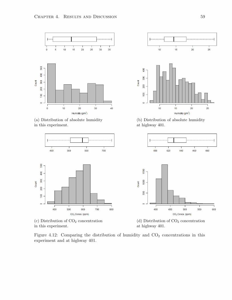
4.12 Comparing the distribution of humidity and CO2 concentrations in this

experiment and at highway 401. . . . . . . . . . . . . . . . . . . . . . . . 59

4.13 Comparing the reference CO2 concentrations and sensor measurements. . 60

4.14 Diurnal patterns of CO and CO2 concentration . . . . . . . . . . . . . . 62

4.15 Comparison between time series concentrations in medical air and outdoor

air. . . . . . . . . . . . . . . . . . . . . . . . . . . . . . . . . . . . . . . . 63

4.16 Diurnal patterns of O3 and NOx concentration . . . . . . . . . . . . . . . 65

4.17 Diurnal patterns of UFP and BC concentration . . . . . . . . . . . . . . 67

A.1 Comparison between time series CO and CO2 concentration in Compressed

Air and outdoor air at Wallberg Building. . . . . . . . . . . . . . . . . . 81

A.2 Comparison between time series O3 and NOx concentration in Compressed

Air and outdoor air at Wallberg Building. . . . . . . . . . . . . . . . . . 82

B.1 NOx and O3 in outdoor air Vs. in medical air . . . . . . . . . . . . . . . 84

ix

Chapter 1

Introduction

1.1 What is Medical Air

Medical air is an odorless, tasteless, colorless gas with a similar composition to the air

we breathe. It is comprised of about 78% nitrogen, 21% oxygen, and 1% of other compo-

nents such as water vapor, carbon dioxide, hydrogen, and argon [1]. Such air is produced

or conditioned for breathing purposes on-site in hospitals and dental surgeries [2]. It is

considered to be a therapeutic product by the United States Pharmacopoeia (USP) and

is named medical air USP or Air USP [3].

Medical air USP is primarily used for long-term life support such as in intensive care,

neonatal intensive care, and critical care units. It is used in respiratory therapies such

as ventilation, high flow nasal cannula therapy, inhaled nitric oxide delivery, aerosolized

medicine, and pulmonary drug delivery [4]. The quality of medical air is important,

because it is intended for infants, the elderly, and other vulnerable populations [3].

1.2 How is Medical Air Produced

Medical air is most often produced on-site in hospitals and healthcare institutions by

pulling outdoor air into Medical grade compressors, filtering and drying the compressed

air, and distributing it in the hospital’s piping system. However, if the outdoor air quality

1

Chapter 1. Introduction 2

is poor or when only a small amount of air is required, medical air is produced by mixing

pure oxygen and nitrogen and is stored inside cylinders. In general, on-site production is

more practical and economical for the large volumes of air consumed in hospitals. The

downside of on-site manufacturing is that it requires a more complex and costly design

which must be installed and maintained carefully to keep patients safe and minimize the

risk of contamination [5].

The complexity of the medical air system and the purity of the produced air is un-

clear to most healthcare staff [5]. Any undesired gases or impurity in the air entering the

system will be compressed and delivered to the patients, unless it is removed through

the compression and the filtration system. In one instance, hospital staff reported that

a bird was drawn into the medical air system and patients had complained about the

odor resulted from the decaying bird [5]. Another example is a case where the intake

was located beside an air conditioning system; while cleaning the system with an acidic

solution, the fumes were drawn into the medical air inlet [5]. Based on these examples

and other similar incidences, it can be understood that the composition of medical air

cannot always be confidently known at the hospital bedside end of the distribution sys-

tem. Figure 1.1 shows the medical air system schematically. In the following, we will

discuss each part of the system in more detail.

Figure 1.1: Schematic of the medical air system


1.2.1 Intake for the Medical Air

The location of the inlet has a great impact on the quality of medical air. The National

Fire Protection Association Code 99 (NFPA99) recommends standards for location, de-

sign, and components of medical air systems. Based on this standard, the inlet should

be placed outdoors, on the roof, at least 10ft away from any doors, windows, or other

openings, at least 20ft above the ground, and should be protected against the entry of

water, animals, and insects. In the case of installing multiple compression systems in a

building, NFPA99 allows hospitals to share one intake for all the systems which must

be sized properly, and each system must be designed to be disconnected from the line

safely. If the outdoor air is polluted and indoor air has an equal or better quality, intake

may be located within the building, but the purity must be checked regularly and if the

outdoor air quality has improved the intake should be moved back outdoors [5].

1.2.2 Inlet Filter

The inlet filter should be located before the compressors to remove dirt and coarse parti-

cles from the ambient air. This filter is meant to reduce fouling of the internal compressor

components, increase compressor’s lifespan, and decrease the end line filters’ workload

and operation noise. However, NFPA99 does not mandate the installation of this piece

of equipment in the medical air system [5].

1.2.3 Air Compressor

The compressing system increases ambient air pressure by 8 times. Usually, more than

one compressor is installed to provide the required volume of medical air in an average

hospital, and a backup system is provided for the case if one unit needs maintenance

[5]. Each compressor must be provided with appropriate valves to be insulated from the

system for servicing. Each unit must be capable of producing an adequate volume of air

at the maximum demand [5].

The medical air system is designed to produce air used exclusively for breathing


purposes and should not be used for non-medical applications. Such use can increase the

demand on the system, reduce system lifetime, and open new sources of contamination to

the system. Based on NFPA99, the installed compressors must not introduce oil droplets,

water, or toxic oil products into the medical air, or the system must be designed to

separate out these contaminants [5].

1.2.4 After-Coolers

The after-cooler is an optional piece of equipment installed based on the system design

to lower the temperature after the compression system. They should be equipped with

water traps to drain the condensed water and isolation valves, so that after-coolers can

be disconnected without shutting down the whole system [5].

1.2.5 Receiver

The receiver is a cylinder that stabilizes the air pressure after compression. The receivers

should be provided with a pressure relief valve, sight glass, pressure gauge, and a water

trap to drain condensed water. While stainless steel cylinders are recommended, NFPA99

permits the iron receivers, which may rust and make flakes into the air [5].

1.2.6 Air Dryer

Dryers remove condensed water after the air passes through the compressing system.

They are mostly of the desiccant or refrigerant type. Desiccant dryers have a bed of

absorbent material, normally made from Activated Alumina, which removes the moisture

from the air stream. While only one dryer works at a time, two dryers must be installed

to allow for service maintenance and recovery. Each dryer should be able to handle the

peak load and have a bypass valve for disconnection during servicing [5, 6].

1.2.7 Final Line Filters

Final line filters prevent entry of upstream particles, oil droplets, and odor into the hos-

pital’s distribution system. Each of the filters must be sized to work with 98% efficiency


at 1 micron and handle 100% of the peak system demand at the design condition. As

a result of compression, all the pollutants such as particulate matter, pollen, water, and

gaseous pollution are concentrated. Final filters are capable of removing particulates;

however, water can pass through filters and make its way to patient rooms. Also, special

scrubbers may be required to remove CO in more polluted environments [5]. Neverthe-

less, in most cases, no gas-specific filters are installed in medical air system, meaning any

outdoor gas pollution may be delivered to the patients.

1.2.8 Air Quality Monitoring System

Air quality monitoring systems are installed after the final filters and are intended to

measure pollutants at concentration levels of the USP standards, which can be orders of

magnitude higher than the normally encountered levels in outdoor air. The specifications

of this system is not mentioned in the standards.

1.2.9 Alarms

An alarm will be activated visually and audibly if concentrations rise above the USP

standard thresholds or if the downstream pressure is outside the desired range [5]. The

warning signals should be available to all the building services.

1.2.10 Final Line Regulators

Final line regulators are one of the most important parts of the system, as they adjust

the air pressure throughout the building. The final pressure should be reduced from

80− 100psig to 50− 55psig before entering the hospital’s piping system [5].

1.2.11 Piping

The material used for pipelines should be non-corrosive and resistant to water conden-

sates, such as copper and brass [5]. Copper also has an antibacterial effect and as such

is more preferred. The piping between the compressor, dryer, receiver, and after-cooler

also must be non-corrosive [5].


1.3 Typical Sources of Contamination

Contamination might enter the medical air from several sources, the more common ones

being:

• Water can pass through the filters and contaminate the air or damage equipment.

• Water contamination may result from dryer saturation or inadequate maintenance,

failure of the automatic drains, or if the compressors malfunction.

• Oil can be introduced to the medical air after compression, due to malfunctioning

of compressors or installing inappropriate compressors.

• Sand, solder, and dirt may enter medical air due to poor construction techniques.

• Metal elements might enter medical air from welded parts of the pipelines.

• Filters might have limitations in removing nanoparticles.

1.4 Medical Air Standards and Their Shortcomings

Compared to Outdoor Standard Specifications

Canadian commercial producers of medical air and hospitals are mandated to validate

the quality of their final product to USP specifications. However, these standard regula-

tions are inadequate to meet the requirements of patient’s health and safety. This is due

to three main limitations: specifications allow for higher concentration of air pollutants

than outdoor standards, do not include all the conventional pollutants, and do not spec-

ify the allowable exposure time.

Most often outdoor air is assumed to be clean enough for sensitive populations, to

breath it from several hours to a few months [7]; however, previous studies have shown

the adverse effects of outdoor air pollution on patients, which will be discussed in the next

chapter. Medical air standards are less stringent than outdoor regulations, allowing for


higher levels of air pollution exposure, which is inappropriate for sensitive patients. As

an example, standard thresholds of CO, NOx, and SO2 in medical air are multiple times

higher than ambient air quality standard. Also, ozone is a common air pollutant which

is unspecified in medical air standards. In addition, the time period of exposure to the

maximum level of pollutants should be specified in these standards. Finally, the medical

air standard of 500 ppm for CO2 is very close to the level above 400 ppm typical of

outdoor air, making exceedances quite likely. Table 1.1 compares standards for outdoor

air quality with medical air standards.

Table 1.1: Comparing medical air and ambient air quality standards

Pollutant Ambient Air [9] Medical Air [8] Ratio

Averaging Time Level (ppb) (ppb) (Medical

Ambient)

SO2 1hr 70 5,000 71

NO2 1hr 60 2,500 41

CO 8hr 9,000 [10] 10,000 1.1

CO2 - N/A 500,000 -

O3 8hr 62 N/A -

1.5 Potential Hazards in Using Medical Air

Most of the studies investigating the factors associated with the quality of medical air

have focused on two main concerns: breathing cold and dry air and inhaling uncontrolled

concentrations of oxygen. These problems can cause both long and short-term adverse

effects on neonates and susceptible adults.

An unconditioned, cold, and dry mixture of medical air and oxygen is usually used in


resuscitation of infants during the first minutes of their life [11, 12], which may decrease

pulmonary compliance and conductance during short-term exposure while longterm ex-

posure can result in serious lung injuries and reduction in infants’ core body temperature.

Exposure to dry medical air also contributes to tension and deformation of the lung cells,

ciliary function disorders, high mucus viscosity, and lung inflammation and during short-

term exposure proves detrimental to the mucosal cells in adult patients [13, 14, 15].

Oxygen is the essential component in most of Medical gas mixtures. Too short an

exposure or a decrease in oxygen concentration might damage patients’ organs or cause

death, and too long an exposure or excessive concentration of oxygen is associated with

increased morbidity and mortality in very low birth weight infants. Long-term use of

high oxygen concentration also results in permanent blindness in premature neonates

caused by overgrowth of blood vessels in their eyes [16, 17].

Medical air is used for ventilating incubators and supporting neonates’ breathing after

birth. Most preterm births occur in the last weeks of gestation when the most rapid lung

maturation occurs. Preterm lungs continue growth after birth and their maturation is

highly affected by air pollution exposure. Chemical exposure during fetal development

and postnatal life can delay the lungs’ development and is associated with many long

and short-term health problems such as abnormal lung development, low and very low

birth weight, preterm birth, congenital defects, childhood asthma, behavioral problems,

neurocognitive decrements, and infant mortality [18, 19].

Previous studies have suggested that air pollution may enhance the risk of asthma,

chronic obstructive pulmonary diseases (COPD), lung cancer, respiratory infections, and

cardiovascular disorders in more susceptible populations such as infants, children, and

the elderly [19, 20]. Among all the chemical air pollutants PM2.5, ozone, and nitrogen

dioxide have the most exacerbating health effects [20]. In the following chapter, we will

discuss the health effects of these common pollutants.


1.6 Previous Studies on the Quality of Medical Air

Only in recent years has there been study on the quality of medical air. Potentially

the first serious discussion and analysis of pollution levels in medical air were performed

by Benzing et al. (1999), who observed clinically significant concentrations of nitrogen

oxide (> 80ppb) in the compressed air at a university hospital during 40% of the working

days [21]. Unintentional inhalation of nitric oxide had caused lung damage to patients.

In addition, Nakata et al. (2002) showed that the concentration of NOx and CO in

medical air peaked during rush hours [22]. Yet, the relationship between outdoor air

quality and pollution concentration in the medical air is unknown. Recently, Edwards

et al. (2018) measured the carbon dioxide concentration in the medical air produced on-

site at a Canadian hospital, and demonstrated that the level of carbon dioxide exceeded

the USP standard threshold for 1% of the total test period [4]. The current research

investigated the effect of outdoor pollution on the medical air quality in the patient

rooms by deploying low-cost sensors and portable devices near the air intake and at the

outlet of the medical air.


1.7 Thesis Summary and Objective of the Chapter

Medical air is defined as a therapeutic medicine, commonly produced on-site at health-

care facilities. The medical air system takes the outdoor air, compresses, dries, filters out

particulates, and delivers the produced air to patients. However, usually no filters are

installed to remove gaseous pollution. The quality of medical air is monitored after man-

ufacturing and an alarm goes off if the pollution levels exceed the standard thresholds;

however, patients’ exposure is not monitored continuously at the endpoint. Maximum

allowable pollution concentration in medical air is regulated by the United States Phar-

macopoeia. These standards do not include all common outdoor air pollutants, allow for

far higher concentrations than outdoor standard levels, and do not specify the allowable

exposure time. Previous studies have shown considerable levels of pollution in medical

air, which was associated with adverse health outcomes.

The main objectives of this research were to deploy low-cost sensors at hospitals and

investigate the relationship between outdoor air pollution and the medical air quality.

Chapter 2 synthesizes relevant literature to provide context. The methodology developed

and applied is described in Chapter 3. Results are discussed in Chapter 4 and Chapter

5 concludes the project.

Chapter 2

Literature Review

2.1 Health Impacts of Air Pollution

2.1.1 Particulate Matter (PM)

Particulate matter (PM) is emitted from both human and natural activities. Human

activities include wood and fuel combustion, agricultural operations, transportation,

construction, biomass burning, and industrial processes. A significant portion of PM

is generated from natural sources such as wildfires and dust winds [23, 24]. Exposure

to PM has negative impacts on human and animals’ health, ecosystems, and visibility,

and it is estimated to cause millions of deaths annually [23, 26]. Exposure to low con-

centrations of PM is associated with heart disease and stroke; with a stronger risk for

women than for men, for non-smokers than for smokers, and for higher socioeconomic

classes [27]. Annual global average concentration of PM is approximately 7µg/m3 [25];

however, previous studies have suggested strong links between various syndromes, such

as attention deficit hyperactivity disorder, autism, loss of cognitive function, anxiety,

asthma, COPD, and hypertension with PM exposure [26]. Long-term exposure to high

levels of PM is associated with a range of respiratory and cardiovascular diseases, Parkin-

son [28, 29], cell death mechanism disorders, DNA damage, and a higher risk of cancer

[28]. Prenatal exposure to PM adversely affects microRNAs (miRNAs) by altering gene

expression profile, which may have long-term health outcomes in their later-life [30, 31].

11

Chapter 2. Literature Review 12

In addition, short-term exposure to PM2.5 and PM10 is significantly associated with out-

of-hospital cardiac arrest (OHCA) and mortality, with strongest association being with

PM2.5 [32, 33].

2.1.2 Ozone (O3)

Ozone is a highly toxic, reactive, and oxidative gas associated with an increased risk of a

variety of adverse respiratory and cardiovascular system outcomes, such as asthma, out-

of-hospital cardiac arrest, mis-balancing of autonomic components and arterial pressure

control, oxidative stress, inflammation, coagulation, myocardial infarction, cardiac auto-

nomic disorders, arrhythmia, and a rise in the rate of mortality and morbidity [33, 34, 35].

Epidemiological evidence has estimated that 16,000 premature deaths were related to o-

zone exposure in European Union in 2013 [35]. Ozone is an important factor of increased

risk in asthma with a higher vulnerability in children [36]. Air pollution monitoring sites

worldwide show that ozone concentration often exceeds the World Health Organization

(WHO) regulated standard level for the human health protection [35]. Daily 8-hour

exposure to the maximum allowable ozone concentration and the number of patients

suffering from asthma are significantly correlated for all ages [36]. Despite the negative

health impacts of ozone, the USP standards do not include safe levels of this pollutant

for sensitive populations, and patients’ exposure is not monitored at most hospitals.

2.1.3 Nitrogen Dioxide (NO2)

Nitrogen dioxide (NO2) is an undesirable by-product of combustion in vehicles, industry,

and household gas appliances such as stoves in indoor settings [37, 38]. It has simi-

lar health impacts as ozone, but at higher concentrations [39]. Public health effects of

nitrogen dioxide range from acute symptoms and vulnerability to respiratory infection,

to permanent lung function damage and chronic diseases [38, 40]. Children, asthmat-

ic individuals, and athletes are at a greater risk [39]. Long-term exposure to nitrogen

dioxide enhances the risk of respiratory tract infections, cardiopulmonary diseases, and

lung cancer mortality in non-smokers [41, 42]. In indoor settings, gas cooking with poor


ventilation generates high concentrations of nitrogen oxides [41], which is associated with

an increased risk of asthmatic symptoms including coughs, chest tightness, breathless-

ness, and asthma attacks [40, 38]. Epidemiological studies have indicated that exposing

children to hourly peak levels of 80ppb NO2 is connected to adverse respiratory effects

[43, 44]. These impacts may or may not be specific to NO2 as NO2 has often been used

in epidemiology as a marker of exposure to the complex mixture that makes up traffic

related air pollution. Although nitrogen dioxide has been associated with adverse health

outcomes at levels encountered outdoors, its allowable concentration in medical air is far

above the ambient air quality standards.

2.1.4 Sulfur Dioxide (SO2)

Exposure to sulfur dioxide (SO2) can affect both healthy and sensitive populations. Based

on findings from laboratory studies of controlled exposure to sulfur dioxide, the US En-

vironmental Protection Agency (EPA) has concluded that short-term exposure to SO2 is

associated with a higher risk of respiratory morbidity [45]. Respiratory effects are report-

ed at moderate (< 500ppb) and high concentrations (> 500ppb) in both healthy patients

and those with pulmonary disease; however, no associated annoyance and lung function

disorders are observed at exposures up to 200ppb in healthy populations; in other words,

studies have not confirmed a clear dose-dependent health risk response to this pollutant

at low concentrations [42, 46].

Exposure to SO2 in pregnancy, perinatal, and postnatal life has more severe health

outcomes. In pregnancy, maternal exposure may cause low birth weight, during perinatal

development may damage the parasympathetic regulation of cardiovascular activity, and

in postnatal life disrupts the neurotransmission to cardiac vagal neurons [47].

2.1.5 Carbon Monoxide and Carbon Dioxide (CO and CO2)

Both carbon monoxide (CO) and carbon dioxide (CO2) are generated from wood and fuel

combustion, emitted from vehicles or indoor heating and cooking appliances. Outdoor


concentrations of CO and CO2 are typically below the standard safe levels of exposure;

however, since people spend about 90% of their time indoors, vehicular pollutant expo-

sure in near-road buildings can be 6-9 times higher than that at road sidewalks [48].

Both CO and CO2 have acute health outcomes at high concentrations, mostly occur-

ing indoors due to poor ventilation and malfunctioning of combustion appliances [49]. A

study in 2007 demonstrated that CO concentration in 67% of households with gas heaters

and 60% of those with wood heaters is above the World Health Organization’s (WHO)

standards [50]. At high concentrations, CO is a toxic inhalation hazard, may cause eye

irritation, dizziness, concentration difficulties, headaches, sensorineural hearing loss, and

even death [51, 52, 53].

Exposure to high levels of CO2 in low oxygen concentration can result in adverse

health effects such as headaches, fatigue, sleepiness, dizziness, poor memory, difficulty

to concentrate and think clearly, tinnitus, loss of eye movement and vision problems,

and personality changes [54, 55]. Long-term exposure to lower concentrations of CO2

in presence of normal oxygen may potentially induce longer-term adverse effects in both

healthy patients and vulnerable populations [54].

2.2 Low-Cost Air Quality Sensors

Compared to traditional methods of monitoring air quality, low-cost sensors have intro-

duced an inexpensive method for collecting large amounts of high spatial and temporal

resolution data. Low-cost sensors are small, portable, easy to install, and can be used

for applications where deploying traditional monitoring devices is likely impossible, such

as measuring exposure levels inside vehicles, public transportation, and trains. However,

calibrating these sensors is a complex challenge [56, 57, 58].

Various calibration algorithms have been developed to increase the accuracy of the

low-cost instruments’ measurements. These calibration models usually use an array of


sensors to account for the cross-sensitivity of different pollutants and the effect of envi-

ronmental parameters. There are three main types of low-cost sensors which are different

in price, pollutant selectivity, and sensitivity: Metal Oxide Semiconductor (MOS), Elec-

trochemical (EC), and optical sensors. In general, the MOS sensors are more affordable

but less selective than the EC and optical sensors. Electrochemical sensors have rela-

tively high selectivity and sensitivity making them proper for measuring a wide range of

pollutants. Optical sensors have an acceptable selectivity, but are moderately expensive

and have a high detection limit. Table 2.1 summarizes the characteristics of the gas

sensors.

Table 2.1: Summary of characteristics of low-cost sensors [59]

SensorRelative

CostSelectivity Sensitivity Typical Pollutants

MOS $ Uncertain Acceptable CO, O3, NO2, NH3

EC $$ Moderate Good CO, O2, NO, NO2, Cl2, SO2, H2S

Optical $$ Moderate Poor CO2, Hydrocarbons, PM

In the following section, we will explain these types of sensors in more detail and

introduce four frequently used calibration models.


2.2.1 Metal Oxide Semiconductor (MOS) Sensors

These sensors usually have an internal heater and an active sensing element made of

tin oxide or aluminum oxide. The sensing mechanism occurs through reactions between

oxygen and pollutant molecules on the surface of the sensing element at high temperatures

(300-500 ◦C). Molecular oxygen is adsorbed to the surface and forms O2-, O-, or O2-

and reacts with the gas molecules [60]. These reactions cause measurable changes in the

electrical conductivity, which can be related to the pollution concentration [59]. Typically,

MOS sensor’s response has a nonlinear relationship with the pollution level, which makes

their calibration more sophisticated [59]. Figure 2.1 shows the sensing mechanism of

MOS sensors.

Figure 2.1: Sensing mechanism of MOS sensors [59]


2.2.2 Electrochemical (EC) Sensors

These sensors are based on oxidation-reduction reactions between pollutant molecules

and the electrodes within the sensor. There are three electrodes inside the small sensor’s

chamber: the working, counter, and reference electrodes. The working electrode is coated

with a catalyst to provide a high surface area for a reduction or oxidation reaction with

the gas molecules. The electronic charge generated on the working electrode balances

with a reaction on the counter electrode to form a pair of redox chemical reactions,

which produces a measurable current proportional to the pollutant concentration. The

reference electrode is used to maintain the working electrode at a constant electrical

potential during the sensing operation, and the counter electrode has a floating potential

to compensate for the generated current at the working electrode [61]. The opening of

the sensor has a gas-permeable membrane which prevents the electrolyte to leak from

the small chamber and decreases the interference of unintended pollutants [59]. Figure

2.2 illustrates the schematic of an electrochemical sensor.

Figure 2.2: Schematic of electrochemical sensors [59]


2.2.3 Optical Sensors

These sensors consist of a light source, band-pass filter, a sample chamber, and a detector.

They work based on sensing the deviation or absorption of light at a specific wavelength.

Light deviation is usually used to measure particulate matter, and absorption is applied

to monitor gaseous pollutants.

The Beer-Lambert law is used to quantify atmospheric pollutant levels when measured

with an optical sensor:

I = I0exp(−σ ×N × b) (2.1)

Where I0 and I are light intensity before and after crossing a sample, respectively, σ

is absorption cross-section (m2), N is concentration of the absorbing gas (molecule/m3),

and b is the length of the light path (m) [59]. One limitation of this type of sensor is its

large detection limit (> 10ppm), which makes it inappropriate for measuring atmospher-

ic levels of most pollutants [59]. Also, compounds with close absorption wavelengths

can interfere with each other. For example, water vapor interferes with measuring CO2

concentration. Figure 2.3 shows a schematic of these sensors.

Figure 2.3: Schematic of optical sensors [59]


2.3 Machine Learning Algorithms Used for Calibrat-

ing Sensors

While some sensors directly convert their output to a digital pollutant concentration

measurement, the outputs of most sensors are voltages or numbers proportional to the

pollutant levels. These outputs need to be related to actual concentrations through

Machine Learning algorithms. Four common models are explained here:

2.3.1 Multiple Linear Regression (MLR)

Multiple Linear Regression (MLR) is a method used to model a linear relationship be-

tween the concentration and one or more sensor outputs. This model is fit such that the

sum of squares of the differences between the observed values and predicted concentra-

tions is minimized [62].

Observed data→ y = b0 + b1X1 + ...+ bnXn + ε (2.2)

Predicted data→ y′= b0 + b1X1 + ...+ bnXn (2.3)

error→ ε = y − y′(2.4)

Minimize∑

(y − y′)2 (2.5)


This model has four assumptions:

• The outcome variable and the independent variables have a linear relationship with

each other.

• The residuals are normally distributed.

• The independent variables are not highly correlated with each other.

• The variance of errors is similar across the values of the independent variables.

This model usually works very well for electrochemical sensors; however, since the

assumptions are not always valid for a combination of EC and MOS sensors or for an

array of MOS sensors, non-linear models are usually more preferred.

2.3.2 Random Forest (RF)

Random Forest (RF) consists of several Decision Trees with a random subset of indepen-

dent variables. Every Decision Tree breaks down the dataset into smaller subsets and

finds rules to predict the target. The results of all the trees are averaged to make the

final decision. Figure 2.4 shows a Random Forest.

One problem with RF is that it can only predict values within the range of training

set, thus usually is not transferable from one place to another. For example, an RF model

trained on an unpolluted area is unable to estimate the peak values in a polluted area.


Figure 2.4: Schematic of a Random Forest algorithm [63]

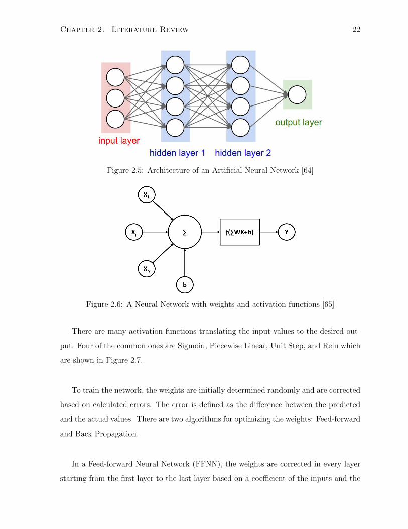
2.3.3 Artificial Neural Network (ANN)

Artificial Neural Networks replicate the biological neural network of a living brain. It

is comprised of several layers of artificial neurons (or nodes) connected to each other to

form a network. There are three types of layers: input, hidden, and output layers. A

Neural Network has one input layer, one output layer, and one or more hidden layers.

Figure 2.5 shows a typical network architecture.

The input data enters from the input layer and passes to the hidden layer. The values

are multiplied by weights when passing between nodes. Each node sums the values it

receives and modifies based on an activation function. This process continues to the

last layer of the network, which represents the final value; in our case is the predicted

concentration. Figure 2.6 shows how a Neural Network works.


Figure 2.5: Architecture of an Artificial Neural Network [64]

Figure 2.6: A Neural Network with weights and activation functions [65]

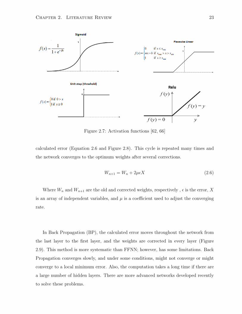
There are many activation functions translating the input values to the desired out-

put. Four of the common ones are Sigmoid, Piecewise Linear, Unit Step, and Relu which

are shown in Figure 2.7.

To train the network, the weights are initially determined randomly and are corrected

based on calculated errors. The error is defined as the difference between the predicted

and the actual values. There are two algorithms for optimizing the weights: Feed-forward

and Back Propagation.

In a Feed-forward Neural Network (FFNN), the weights are corrected in every layer

starting from the first layer to the last layer based on a coefficient of the inputs and the


Figure 2.7: Activation functions [62, 66]

calculated error (Equation 2.6 and Figure 2.8). This cycle is repeated many times and

the network converges to the optimum weights after several corrections.

Wn+1 = Wn + 2µεX (2.6)

Where Wn and Wn+1 are the old and corrected weights, respectively , ε is the error, X

is an array of independent variables, and µ is a coefficient used to adjust the converging

rate.

In Back Propagation (BP), the calculated error moves throughout the network from

the last layer to the first layer, and the weights are corrected in every layer (Figure

2.9). This method is more systematic than FFNN; however, has some limitations. Back

Propagation converges slowly, and under some conditions, might not converge or might

converge to a local minimum error. Also, the computation takes a long time if there are

a large number of hidden layers. There are more advanced networks developed recently

to solve these problems.


Figure 2.8: Feed Forward Neural Network

Figure 2.9: Back Propagation

Where X1 to Xn are input data, W1i to Wni are weights of the first to the nth nodes,

f is activation function, y′

is output of the network, and y is the reference measurement.

In BP, the weights are corrected using the output of the layers and the calculated

error:

Wn+1 = Wn + µδX (2.7)

Where Wn and Wn+1 are the old and corrected weights, respectively , µ is a coefficient


to adjust the converging rate, X is the input to every later, and δ is a function of error

and the output at every layer.

2.3.4 Recurrent Neural Network (RNN)

A Recurrent Neural Network (RNN) uses the previous predicted values to make a new

prediction. This algorithm is usually used for time series data, where the previous mea-

surements can affect the future values. For example, pollutant concentration at time tn

is affected by the concentration at time tn-1. The figure below shows the architecture of

this network.

Figure 2.10: Recurrent Neural Network

Where x0 to xn and y’0 to y’n are the inputs and predictions at each sequence, re-

spectively.

The challenge in using this calibration model is to decide an appropriate number of

previous predictions and training iterations. Applying too many of the previous pre-

dictions might bring some errors to the final prediction. Also, training the model for

excessive times might overfit the network on the training set.


2.4 Summary of the Chapter

In this chapter we reviewed the health effects of air pollution with a focus on premature

neonates. Among common pollutants, PM2.5 and NO2 have the most acute outcomes.

We introduced three types of low-cost sensors. Metal Oxide Semiconductor sensors work

based on changes in the conductivity of their active surface. Electrochemical sensors

are based on reduction-oxidation reactions between pollutants and the electrodes inside

the sensor, and optical sensors are based on light deviation or absorption at a specific

wavelength. Lastly, we introduced four common algorithms used to calibrate low-cost

sensors.

Chapter 3

Methodology

3.1 Study Site

This research was conducted at a Canadian hospital located on the corner of two major

roadways and close to a highway. The sampling was performed near the air intake on

the third floor and from a medical air outlet in a patient room on the fourth floor for ap-

proximately seven months from November 2017 to June 2018. The concentration of CO,

CO2, nitrogen oxides (NOx), O3, Black Carbon (BC), and ultrafine particles (UFP) were

monitored on both locations simultaneously. The gaseous pollutants except CO2 were

monitored by a low-cost air pollution measuring device known as AirSENCE, which is

equipped with several Metal Oxide, two Electrochemical, and temperature and Relative

Humidity (RH) sensors. Carbon Dioxide was monitored by an optical sensor independent

from the AirSENCE. Black Carbon and UFP were measured using microAeth and DiS-

Cmini particle counter, respectively. To monitor the medical air, all the portable devices

were placed inside a sampling box connected to an outlet (Figure 3.1 a and b). Electro-

chemical and optical sensors work at atmospheric pressure, so the box was designed to

attenuate high pressure of medical air. It was about 130 liters, equipped with an inlet

and an outlet valve to control the air flow, and a pressure gauge to ensure the internal

pressure is at atmospheric level. Table 3.1 demonstrates the specification of the sensors

and the portable devices.

27

Chapter 3. Methodology 28

(a) Sampling box connected to a med-ical air outlet.

(b) Portable devices were placed insid-e the sampling box.

Figure 3.1: Sampling box

Table 3.1: Specifications of the portable devices

Instrument Target Pollutant Time Resolution

AirSENCE NO, NO2, CO, O3 1 sec

Senseair K30 CO2 2 sec

microAeth BC 10 sec

DiSCmini UFP (10-300 nm) 10 sec


Table 3.2: List of sensors applied to this study

Sensor Name Target PollutantSensor

Type

Interfering

Pollutant

Senseair K30 CO2 Optical Water vapor

Plantower PMS

7003PM10, PM2.5, PM1 Optical -

DHT22Temperature, Relative

Humidity- -

NO-B4 NO EC

H2S, NO2,CL2,

SO2, H2, CO,

NH3, CO2, O3

[67]

CO-B4 CO EC

H2S, NO2,CL2,

NO, SO2, H2,

C2H4, NH3 [68]

MQ131 O3 MOS -

MiCS-5521CO, Hydrocarbons, Volatile

Organic CompoundsMOS -

MiCS-5524 CO, H2,NH3,CH4, Ethanol MOS -

MiCS-5526 CO, H2,NH3,CH4, Ethanol MOS -

MiCS-4514

ReductionCO, Hydrocarbons MOS -


MiCS-4514

OxidationNO2 MOS O3

MiCS-2614 O3 MOS -

MQ-3Alcohol, Benzene, CH4,

Hexane, LPG, COMOS -

SN706 NOx MOS -

TGS2620

CO, CH4, H2, Ethanol,

Iso-butan, Organic Solvent

Vapors

MOS -

TGS2600

CO, CH4, H2, Ethanol,

Isobutane, Organic Solvent

Vapor

MOS -

TGS822

CO, CH4, n-Hexane,

Benzene, Ethanol, Acetone,

Iso-butan, Organic Solvent

Vapor

MOS -


3.2 Sensor Calibration

3.2.1 Calibration Site and Instrumentation

All the portable devices were calibrated beside reference instruments for two weeks at the

Wallberg Building, at a height of approximately 15 meters, in downtown Toronto prior to

deploying at the hospital. The reference instruments represent accurate concentrations

and are calibrated regularly. Table 3.2 lists these reference instruments.

Table 3.3: Reference instruments

Instrument Target Pollutant

NOx Thermo 42i NO, NO2

Thermo 49c O3

LICOR LI-840A CO2, H2O

Thermo 48i-TLE CO

3.3 Data Analysis

3.3.1 Data Preparation

Prior to performing any data analysis, all the negative, extremely large, or false mea-

surements were removed. There are two main steps before training and deploying a

calibration model: averaging and scaling. Averaging alleviates the noise and increases

the confidence; however, averaging to a low time resolution might omit instant variations.

In our study, a 5-minute time resolution was reasonable for keeping the detail of events

while reducing the noise.

Scaling is a very important step when building a neural network model. It makes


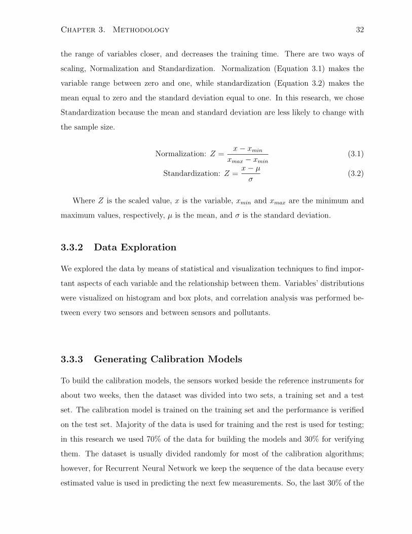
the range of variables closer, and decreases the training time. There are two ways of

scaling, Normalization and Standardization. Normalization (Equation 3.1) makes the

variable range between zero and one, while standardization (Equation 3.2) makes the

mean equal to zero and the standard deviation equal to one. In this research, we chose

Standardization because the mean and standard deviation are less likely to change with

the sample size.

Normalization: Z =x− xmin

xmax − xmin

(3.1)

Standardization: Z =x− µσ

(3.2)

Where Z is the scaled value, x is the variable, xmin and xmax are the minimum and

maximum values, respectively, µ is the mean, and σ is the standard deviation.

3.3.2 Data Exploration

We explored the data by means of statistical and visualization techniques to find impor-

tant aspects of each variable and the relationship between them. Variables’ distributions

were visualized on histogram and box plots, and correlation analysis was performed be-

tween every two sensors and between sensors and pollutants.

3.3.3 Generating Calibration Models

To build the calibration models, the sensors worked beside the reference instruments for

about two weeks, then the dataset was divided into two sets, a training set and a test

set. The calibration model is trained on the training set and the performance is verified

on the test set. Majority of the data is used for training and the rest is used for testing;

in this research we used 70% of the data for building the models and 30% for verifying

them. The dataset is usually divided randomly for most of the calibration algorithms;

however, for Recurrent Neural Network we keep the sequence of the data because every

estimated value is used in predicting the next few measurements. So, the last 30% of the


calibration data was used for testing RNN model.

The R programming language was used to build Multiple Linear Regression, Random

Forest, and Neural Network models, and Recurrent Neural Network was built in Python,

using the Tensorflow library. The models were compared, and the best one was chosen

based on the R2 value and how the model tracks the reference instrument. The sensors

used in every model were initially determined by a function named ”regsubsets” in the

Leaps package in R, which takes a random set of variables and calculates the adjusted

R2 of the best fitted model several times. Then sensors were added or removed step by

step to find the best combination of variables.

3.3.4 Evaluating Calibration Models

To evaluate the calibration models we applied them on the test set and fit a linear model

on the scatter graph of the predicted values against the reference instrument. The slope

of the line represents accuracy of the calibrated model, and ideally should be one, which

means the reference instrument and the model estimate the same values. The intercept

compares the model’s baseline with the reference data, with a large intercept indicating

majority of the predicted values are above or below the actual concentration. R2 of the

line represents how much of the variability is accounted by the model, with a R2 closer

to one indicating the model can predict a large portion of variability of the dataset.

Also, the Root Mean Squared Error (RMSE) of the calibration models were compared

to choose the best model.

3.4 Calibrating CO2 Sensors

We calibrated a Senseair K30 CO2 sensor under laboratory conditions using CO2 cali-

bration gas. The effect of humidity on the sensor’s readings was tested under controlled

conditions. Also, calibration models were built based on environmental temperature,

relative humidity, and pressure.


3.4.1 Investigating the Effect of Humidity on the CO2 Sensor

Optical low-cost CO2 sensors work based on absorbing light at infrared wavelengths.

Water vapor has a strong absorption close to this wavelength and can interfere with CO2

readings. To test the effect of humidity on the Senseair K30 sensor, a vaporizer was

placed beside the temperature, RH, and the CO2 sensor inside the sampling box. The

medical air valve was opened for several minutes to fill the box, and then the inlet and

outlet were closed. Then the CO2 sensor was allowed to work for about 5 min before

turning on the vaporizer to find the initial readings. Then the vaporizer was repeatedly

turned on for about 30 sec, then off for 2 minutes to slowly increase the humidity. The

signals were averaged in every step and changes in the reported CO2 concentration were

observed to see how vapor interfered based on the Beer-Lambert law.

3.4.2 Calibrating CO2 Sensors Under Real Conditions

Two different sites with different concentrations and available reference data were used

for calibration and evaluation of the models. The first site was located at the Wallberg

Building, and the second site was next to the highway 401, in Toronto. A Random

Forest and a Multiple Linear Regression were trained and tested on the data, and the

improvement of the readings and transferability of the models were evaluated at both

sites.


This study was performed at a hospital near highway, and portable low-cost devices

were used to measure the concentration of NOx, O3, CO, CO2, BC, and UFP. The gas

sensors’ outputs were calibrated against reference instruments prior to starting the study.

Four calibration algorithms were trained at Wallberg Building and the best model was

chosen based on RMSE, R2, and scatter plot of the estimated values against the reference

instruments. The effect of humidity on the CO2 sensor was studied under controlled and

real conditions.

Chapter 4

Results and Discussion

4.1 Exploring Calibration Data

Carbon monoxide, carbon dioxide, and nitrogen oxides concentration distributions at the

calibration site are positively skewed. Carbon monoxide concentration varies over a wide

range from less than 100ppb to 500ppb, with outliers spreading to 800ppb, while carbon

dioxide level is mostly focused around 420ppm. The concentration of nitrogen oxides

mostly ranged from about 7ppb to 20ppb, which is above the detection limit of the NOx

sensors (> 5ppb). Ozone had a wider distribution ranging from > 5ppb to about 60ppb.

Temperature and RH had a quite broad range from 5 ◦C to 25 ◦C and 30% to 90%,

respectively. Histogram and box plots of the pollutants are shown in Figure 4.1.

35

Chapter 4. Results and Discussion 36

Figure 4.1: Histograms and box plots of pollutants concentration at the calibration site.


The two AirSENCE devices used in this study, were equipped with different sets of

sensors. AirSENCE #1 had an Electrochemical CO sensor (CO-B4) which is not includ-

ed on the other device, while AirSENCE #2 contained more metal oxide CO and NOx

sensors.

Electrochemical sensors have two outputs, from a working electrode (WE) and auxil-

iary electrode (AE). The WE output was correlated with temperature and the pollutant

concentration, whereas AE was also exponentially proportional to temperature and used

to correct the WE readings. Temperature was a determining parameter affecting sensor

performance and was correlated with both Electrochemical and Metal Oxide sensors.

Ozone was one of the key interfering pollutants, correlated with most of the sensors,

especially NO and NO2. The MOS sensors were mostly correlated with ozone, nitrogen

dioxide, and carbon monoxide. Also, some of the MOS sensors were strongly inter-

correlated, indicating their cross-sensitivity to different pollutants. Figure 4.2 shows the

correlation analysis between all sensors and pollutants.


(a) AirSENCE #1

(b) AirSENCE #2

Figure 4.2: Correlation matrix of all sensors and pollutants.


4.2 Feature Selection

The features were initially selected based on correlation analysis and the results from the

regsubsets function. This function uses maximum likelihood method to build a search

tree for finding the best fitting models of different sizes and builds an MLR model on

each subset. Figure 4.3 shows the output of this function. Each row in these graphs

represents a model; the shaded rectangles in the columns indicate the variables included

in the given model. The numbers on the left margin are the adjusted R2 values in

order; the highest and the lowest numbers represent the maximum and the minimum R2s

achieved, respectively. The darkness of the shading simply represents the ordering of the

R2 values. As an example, the red bar shown in Figure 4.3 b indicates a model which has

an adjusted R2 around 0.93 and its variables are Temperature, MiCS5121, MiCS4514 OX,

TGS880, MiCS2614 1, and MiCS2614 2. The sensors that have no shading were a weak

predictor of the target pollutant and were not selected in any of the subsets, such as

TGS822 and MiCS5526 in this figure.


(a) Ozone on AirSENCE #1 (b) Ozone on AirSENCE #2

(c) Nitrogen Oxides on AirSENCE #1 (d) Nitrogen Oxides on AirSENCE #2

(e) Carbon Monoxide on AirSENCE #1 (f) Carbon Monoxide on AirSENCE #2

Figure 4.3: Results of regsubsets function for selecting models’ independent variables.


The sensors which were more frequently used and had led to a higher R2 were se-

lected as the main features. Other parameters were included if they improved the R2

significantly. Table 4.1 shows the parameters selected for predicting each pollutant.

Table 4.1: Selected sensors for building calibration models

Pollutant AirSENCE # 1 AirSENCE #2

O3

Temperature, TGS2620 Temperature, TGS2620

MQ131, MiCS5524 MiCS5524, MiCS5121

TGS822 MiCS4514-OX, TGS880

TGS2600

NOx

Temperature, TGS2620 Temperature, NO-B4-WE

NO-B4-WE, NO-B4-AE NO-B4-AE, MiCS4514-OX

MiCS4514-OX, MiCS5524 SN706

TGS822

CO

TGS2620, TGS2600 Temperature, TGS2620

MiCS4514-OX, MiCS5524 TGS822, MiCS5524

CO-B4-WE, CO-B4-AE MQ3, TGS880

MQ3 MiCS4514-RED


4.3 Evaluating and Comparing Calibration Models

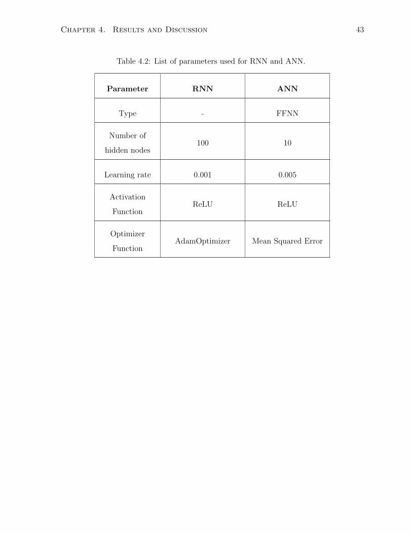
Four calibration models were trained on both devices, the parameters used for RNN and

ANN models are specified in Table 4.2. The R2, slope, and intercept of the predictions

against the reference line, and RMSE were considered for model evaluation and compar-

ison. Table 4.3 indicates the models’ performance on the training set.

Random Forest had the best performance on the training data with the highest R2

(≥ 0.98) and the lowest RMSE for all the pollutants on both devices. The slope of this

model is very close to one (≥ 0.92) and the intercept is small relative to the range of the

pollutants concentration. However, this model cannot extrapolate measurements above

or below the training range [69], and the predictions are usually not transferable from

one place to another, thus it is not preferred over other models.

After Random Forest, Recurrent Neural Network has the highest R2, but its RMSE

is close to MLR, thus this needs to be studied in more detail. Since this model uses the

previous outputs to estimate new measurements, missing values in a dataset can cause

significant errors. Also, this model is prone to overfit on the training data in a few it-

erations. Although Multiple Linear Regression has a comparable RMSE to RNN, it is

more scattered and less accurate. The testing results of these two models were compared.

RNN and MLR were applied on the test set to select the best model for each pollutant.

The results are summarized in table 4.4. Although RNN performs better than MLR on

the training set, its R2 is not as high on the test set, except for NOx on the second device.

The slopes of the two models are close for most of the pollutants, except O3 on device

#1 (RNN: 0.41 and MLR: 0.84) and NOx on device #2 (RNN: 0.95 and MLR: 0.56).

However, MLR has a smaller RMSE for all the pollutants, and the intercept is close to

zero for NOx and O3.


Table 4.2: List of parameters used for RNN and ANN.

Parameter RNN ANN

Type - FFNN

Number of

hidden nodes100 10

Learning rate 0.001 0.005

Activation

FunctionReLU ReLU

Optimizer

FunctionAdamOptimizer Mean Squared Error


Table 4.3: Comparing calibration models’ performance on the training set

Pollutant Model

AirSENCE #1 AirSENCE #2

RF RNN MLR ANN RF RNN MLR ANN

O3

R2 0.99 0.94 0.81 0.43 1.00 0.98 0.94 0.30

Slope 0.96 0.94 0.85 0.79 0.98 0.98 0.94 0.77

Intercept 0.92 1.49 3.71 1.67 0.30 0.42 1.53 4.42

RMSE 1.11 2.98 4.69 11.0 0.67 3.27 1.98 16.9

NOx

R2 0.99 0.96 0.75 0.07 0.98 0.73 0.59 0.13

Slope 0.96 0.95 0.75 0.67 0.92 0.95 0.59 0.36

Intercept 0.63 0.70 4.13 0.07 1.01 -5.27 5.19 6.31

RMSE 1.49 3.27 7.34 37.9 1.78 3.75 7.34 13.5

CO

R2 0.99 0.85 0.76 0.39 0.98 0.90 0.71 0.30

Slope 0.96 0.86 0.76 0.47 0.95 0.93 0.70 0.54

Intercept 0.98 0.90 0.71 140 15.70 24.3 94.30 166

RMSE 11.6 42.7 48.1 78.0 17.5 46.5 73.9 128


Table 4.4: Comparing RNN and MLR’s performance on the test set

Pollutant Parameter

AirSENCE #1 AirSENCE #2

RNN MLR RNN MLR

O3

R2 0.51 0.81 0.89 0.94

Slope 0.41 0.84 0.92 0.93

Intercept 3.71 -0.69 3.71 1.91

RMSE 8.62 4.97 4.73 3.40

NOx

R2 0.41 0.81 0.73 0.58

Slope 0.70 0.84 0.95 0.56

Intercept 24.9 4.12 -5.27 5.45

RMSE 23.34 6.84 9.01 7.66

CO

R2 0.33 0.69 0.42 0.69

Slope 0.67 0.72 0.68 0.70

Intercept 15.7 74.10 85.6 97.9

RMSE 99.2 53.7 86.7 74.3


The box plots of the predictions on the test set were compared with the reference

measurements, which is shown in Figure 4.4. The median, first, and third quantiles of

the MLR model on both AirSENCEs are very close to the reference data for all the pol-

lutants, whereas RNN has a noticeable difference. Also, MLR predictions vary in a closer

range to the reference measurements for NOx and CO and can better estimate the outliers.

Based on all the analyses discussed above, Multiple Linear Regression was selected

and applied to predict the pollutants concentration at the hospital.

(a) Ozone on AirSENCE #1 (b) Ozone on AirSENCE #2

.


(c) Nitrogen Oxides on AirSENCE #1 (d) Nitrogen Oxides on AirSENCE #2

(e) Carbon Monoxide on AirSENCE #1 (f) Carbon Monoxide on AirSENCE #2

Figure 4.4: Comparing box plots of RNN and MLR predictions with the reference mea-surements.


4.4 Calibrating CO2 Sensors

The CO2 sensor was calibrated using calibration CO2 and zero gases. The sensor was

placed inside a small chamber and CO2 concentration was increased from zero to 1000ppm

by 100ppm intervals, while RH and temperature were held constant at around 4% and

22.4 ◦C (Figure 4.5.a). The CO2 reading at each level was averaged and plotted against

the actual concentration, as shown in Figure 4.5.b. The slope and R2 of the fitted line

were very close to one indicating that the sensor is potentially very accurate, but the

intercept was significant.

(a) Increasing CO2 concentration with 100ppm intervals


(b) Measured CO2 concentration Vs. the actual level

Figure 4.5: Calibrating a K30 CO2 sensor using calibration gases.

The CO2 sensor was then calibrated outdoors based on the environmental parameters.

The sensor was operated at a site beside highway 401 for two weeks before the calibration.

Figure 4.6 compares the K30 CO2 readings with the reference measurements and shows

the pressure, temperature, and partial pressure of water vapor (PWater). Pressure was

measured by the reference instrument, while temperature and RH were measured by the

AirSENCE. PWater was calculated from the Antoine Equation:

PSat = 108.07131−

1730.63

233.426 + T (4.1)

PWater = RH × PSat (4.2)

Where PSat is the saturated vapor pressure in mmHg, T is temperature in ◦C, and

the calculated PWater is in mmHg.


Figure 4.6: Pressure, temperature, partial pressure of water vapor, and CO2 level athighway 401 and its comparison to the K30 readings.

An MLR and a RF models were used to correct the sensor readings for the effect of

temperature and water vapor. The slope and R2 of the corrected values against the ref-

erence instrument were 0.86 and 0.98 for MLR and RF, respectively, and the intercepts

were small compared to the range of the concentration (Figure 4.7 a and b). To test

the transferability of the models, they were applied to a data collected at the Wallberg

Building.

K30 CO2 sensor had a built-in Automatic Background Calibration (ABC) algorith-

m that allowed the sensor to dynamically shift its CO2 reading by a constant. This

algorithm compared the minimum reported measurement with the approximate global

average CO2 concentration of 400 ppm and added a value to sensor’s readings. Although

this sensor had an acceptable accuracy without any correction, this algorithm caused two

clusters of data, circled in Figure 4.7 a.


(a) Multiple Linear Regression

(b) Random Forest

Figure 4.7: Calibrating a CO2 sensor based on environmental parameters.


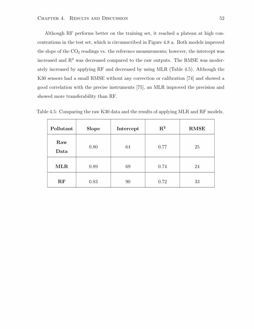
Although RF performs better on the training set, it reached a plateau at high con-

centrations in the test set, which is circumscribed in Figure 4.8 a. Both models improved

the slope of the CO2 readings vs. the reference measurements; however, the intercept was

increased and R2 was decreased compared to the raw outputs. The RMSE was moder-

ately increased by applying RF and decreased by using MLR (Table 4.5). Although the

K30 sensors had a small RMSE without any correction or calibration [74] and showed a

good correlation with the precise instruments [75], an MLR improved the precision and

showed more transferability than RF.

Table 4.5: Comparing the raw K30 data and the results of applying MLR and RF models.

Pollutant Slope Intercept R2 RMSE

Raw

Data0.80 64 0.77 25

MLR 0.89 69 0.74 24

RF 0.83 90 0.72 33


(a) Random Forest

(b) Multiple Linear Regression

Figure 4.8: MLR and RF calibration results Vs. the reference measurements at theWallberg Building.


4.5 Investigating the Cross-Sensitivity of the CO2

Sensor to Water Vapor

To investigate the effect of humidity on the CO2 readings, a vaporizer was placed inside

the sampling box, and humidity was increased gradually (Figure 4.9 a). As the humidity

rose, the sensor detected higher levels of CO2, which indicated its cross-sensitivity to

water vapor. The temperature, relative humidity, and CO2 measurements were averaged

in every constant humidity period (Figure 4.9 b). The CO2 measurements increased from

480ppm to 620ppm by increasing RH from zero to 70%, while temperature decreased for

only about 0.5 ◦C, which is considered negligible. The rise in the CO2 readings should

be proportional to the absorption by water vapor.

The Beer-Lambert law was used to calculate the equivalency in the light wave ab-

sorption of CO2 and water vapor.

Absorption: A = 0.4343×N × σ × b (4.3)

A∆CO2= A∆V apor → N∆CO2

× σ∆CO2= N∆V apor × σ∆V apor (4.4)

Thus: N∆CO2=σ∆V apor

σ∆CO2

N∆V apor (4.5)

Where A is absorption, N is number density of the gas molecules (molec/m3), σ is

absorption cross section, and b is the length of the sample.

The number density of added water molecules has a linear relationship with the num-

ber density of the CO2 molecules which could increase the sensor readings to the same

measurements if were added to the air. The slope of this line is the ratio of vapor to CO2

absorption cross sections. From literature, the absorption cross sections of carbon dioxide

and water vapor at the CO2 absorption wavelength of 4.3 µm are 6.74× 10-24cm2/molec

and 1.20× 10-25cm2/molec, respectively [76].


∆CO2 and ∆V apor at each step were calculated by subtracting the initial CO2 and

RH from their respective values at every point and number densities of gases were calcu-

lated using the ideal gas law. The values used in this experiment are the direct outputs of

the sensor and no calibrations are applied to the measurements. To improve the calcula-

tions, only points 1 to 7 of the CO2 curve in Figure 4.9 b were used to plot N∆CO2against

N∆V apor, and a line of best fit was found for the graph (Figure 4.9 c). The intercept of

this line was forced to zero and the response time of the sensors were removed prior to

calculations.

(a) Effect of increase in RH on CO2 measurements


(b) Average of temperature, RH, and CO2 readings at each step

(c) N∆CO2Vs. N∆V apor

Figure 4.9: Investigating the effect of humidity on the K30 CO2 sensor.


The absorption cross section ratio is 0.0178 and the slope of this line of 0.0174 is

consistent with this ratio given the spread in the data; therefore, our experimental values

match with that expected in theory. At high humidities, vapor condensates can cover

the surface of the light detectors inside the sensor and decrease its sensitivity; points 7

to 9 in Figure 4.9 b show that CO2 measurements deviate from the expected ascending

trend at high humidities.

For more investigation, these calculations were repeated for every period where both

RH and CO2 measurements were falling simultaneously. N∆CO2against N∆V apor graph

is shown in Figure 4.10.

Figure 4.10: Investigating the effect of humidity in the dropping periods.

Part of the data is consistent with the ratio of 0.0178; however, the slope of the best

fit line deviated from the theoretical value, which could be because at higher humidities

the peak CO2 measurements were lower than expected.


This experiment demonstrates the effect of humidity on the sensor outputs; however,

in real conditions, the calibration models should be applied to correct the measurements.

Thus, we applied our calibration model discussed in section 4.4 on this experimental

data.

Figure 4.11: Applying calibration model on the data from the humidity experiment.

This figure shows that the calibration model slightly improved the measurements,

and the difference between the calibrated data and original values increased by increas-

ing humidity; however, ideally the values at high humidities should be close to the first

measurement after calibration. This inefficiency of the model could be because humidity

and CO2 concentrations in this experiment have wider ranges than in real condition-

s. Figure 4.12 compares the distributions of humidity and CO2 concentrations in this

experiment and at highway 401.


(a) Distribution of absolute humidityin this experiment.

(b) Distribution of absolute humidityat highway 401.

(c) Distribution of CO2 concentrationin this experiment.

(d) Distribution of CO2 concentrationat highway 401.

Figure 4.12: Comparing the distribution of humidity and CO2 concentrations in thisexperiment and at highway 401.


Also, sensor measurements under real conditions are very close to the reference values

and follows the variations very well (Figure 4.13 a and b). This makes the calibration

model to significantly relay on the CO2 sensor. Table 4.6 shows the coefficients of the

calibration model. Larger coefficient of the CO2 sensor shows that this parameter is more

influencing the calibrated concentrations.

Table 4.6: Coefficients of the calibration model.

CO2 sensor

(mol/m3)

Humidity

(mol/m3)Temperature

Coefficient 0.98 -0.002 -0.00026

(a) Box plots of the reference CO2 con-centrations and sensor measurements.

(b) Time series of the reference CO2 con-centrations and sensor measurements.

Figure 4.13: Comparing the reference CO2 concentrations and sensor measurements.


4.6 Application to Air Quality Monitoring at the

Hospital and Wallberg Building

After calibration, the sensors’ outputs at the hospital were transferred to concentrations.

The measurements show that only 17% of the outdoor CO was removed in the medical

air system, while CO2 concentration in the outlet was as high as the outdoor air. The

diurnal patterns of CO and CO2 in the medical air were strongly correlated to those

outdoors (0.82 and 0.96, respectively), which is shown in Figure 4.14. Also, the time

series monitoring data of the Medical, shown in Figure 4.15 indicated that the CO and

CO2 concentrations in the medical air and strongly followed the outdoor trend and that

changes in the inlet concentrations were rapidly delivered to the outlet. The CO2 con-

centration in the medical air in 2% of the time passed the USP standard level of 500ppm,

when the outdoor level was at peak; one of the concentration exceedances is indicated in

Figure 4.15.a. This agrees with findings from Edwards et al (2018), who demonstrated

that CO2 level in the medical air exceeds the USP threshold at 1% of the time [4]. The

large confidence interval of the medical air curve in Figure 4.14 shows that CO2 level

varied over a wide range. This could be because the activated alumina used in desiccant

dryers can capture CO2 [70], and release it throughout the course of several days.


Figure 4.14: Diurnal patterns of CO and CO2 concentration


(a) CO2 concentration

(b) CO concentration, USP threshold is 10ppm.

Figure 4.15: Comparison between time series concentrations in medical air and outdoorair.


Although no gas filters were installed in the medical air system, the concentrations of

NOx and O3 were about half of those in the outdoor air. Specifically, 45% and 43%, of

the NOx and O3 , respectively, were removed relative to the outdoor air. Although, their

concentrations had a very small variation, the diurnal patterns of these pollutants in the

medical air were partially related to the outdoor air, which shows that ambient air pol-

lution has affected pollutant concentrations in medical air. For more details please refer

to Appendix B. Unlike, the low concentrations of NOx and O3 observed in this research,

Benzing et al. (1999) and Nakata et al. (2002) measured significant levels of NOx in

medical air [21, 22]. Several parameters could cause this contrast, such as length of the

pipelines and type of the catalysts used in the dryers. NOx can react with atomic copper

and copper (II) oxide (CuO) under certain circumstances [71, 72], and long pipelines can

provide enough residence time for the reactions. In addition, zeolite type desiccants can

absorb nitrogen dioxide at room temperature [73]. Further the outdoor concentrations

of these pollutants may have been higher in these earlier studies. The small confidence

interval of NOx and O3 concentrations in the medical air indicates their small ranges of

variation (Figure 4.16).


Figure 4.16: Diurnal patterns of O3 and NOx concentration


Fortunately, UFP and BC were more than 97% filtered and their correlation to the

outdoor concentrations was low, indicating that the filters were properly working. Their

tight confidence intervals shown in Figure 4.17 illustrates that their concentrations are

around zero most of the time. Table 4.7 summarizes the removal ratio of each pollutant.

Table 4.7: Removal ratio of each pollutant in the medical air.

PollutantRemoval

Ratio

CO2 0.01

CO 0.17

NOx 0.45

O3 0.43

UFP 0.98

BC 0.97


Figure 4.17: Diurnal patterns of UFP and BC concentration



In this chapter we explained four steps of datamining, namely data exploration, building

calibration models, evaluating the models, and deploying them at a new study site.

In data exploration, pollutants were visualized on histogram graphs and a correlation

analysis was performed between all the parameters. To predict pollutant concentrations,

input parameters were selected based on the correlation analysis, and improvement in

R2 of the fitted models. Four calibration models were trained and compared with each

other. The best model was selected based on RMSE of the predictions and reference

measurements and the R2, slope, and intercept of the best fitted line on predictions Vs.

reference values plot. Random Forest had the best results on the training set, however,

does not work as well as MLR at other sites. RNN also has a good performance, but

overfits on the training set, and ANN did not have a high R2 for most of the pollutants,

so MLR was selected to estimate the pollution levels in the inlet and outlet of the medical

air system. A CO2 sensor was calibrated under laboratory conditions and in the outdoor

environment. The CO2 sensor showed promising reliability comparing to the reference

instrument, but is cross-sensitive to water vapor and should therefore be corrected for

the effects of environmental parameters. The results showed that CO and CO2 taken

from outdoors were delivered unchanged to the patient rooms, while NOx and O3 were

more than 40% removed, were still present. Ultrafine particles and black carbon were

more than 97% removed, showing that the particulate filters were working properly in

the medical air system.

Chapter 5

Conclusion and Future Work

The goal of this research was to investigate the effect of outdoor air pollution on the

quality of medical air produced on-site in health care facilities for breathing purposes.

This research showed that low-cost sensors can be deployed at hospitals to monitor the

quality of medical air, and showed that the pollutants concentration in the medical air

is a strong function of the outdoor air quality. Also, this research indicated that the

medical air standards allow for concentrations far above ambient levels, and that levels

of pollution allowed in medical air could potentially cause negative health outcomes. In

the future, the medical air regulations should be revised to include a standard for ozone

and other common pollutants and correct the current limits of other pollutants to be

more aligned fit ambient air quality standards. There seems to be no reason to justify

why hospital patients including neonatal babies should be allowed to experience much

higher exposure to air pollution than the general public.

The next step in this research might be to develop a monitoring setup compatible

with the hospitals’ environment to continuously measure the levels of pollution in med-

ical air in the patient rooms. Being aware of the air pollution concentration in medical

air should help medical professionals make informed decisions on providing a better air

quality for sensitive patients.

One possible solution for purifying the medical air is to install gas pollution filters in

69

Chapter 5. Conclusion and Future Work 70

the medical air system or in the patient rooms. This solution is more suitable in polluted

cities where the outdoor air needs to be continuously cleaned, or at hospitals with an old

medical air system where the produced air is not clean enough for breathing purposes.

Modern commercial filters can remove more than 90% of gaseous pollutants, though they

are expensive and require regular maintenance.

An alternative solution which is applicable for places with better outdoor air quality

is to provide a medical air cylinder at patient rooms to bypass the main system when

the outdoor air pollution exceeds a safe level. In this case, the medical air system work-

s in the same way as the current systems but is able to switch to a cylinder if high

pollutant concentrations are detected in the medical air outlets. However, the prereq-

uisite for this solution is to establish safe levels of air pollution for vulnerable populations.

Chapter 6

References

[1] Medical Air. (n.d.). Retrieved from http://www.gasafrica.com/medical-air.html.

[2] MEDICAL AIR. (n.d.). Retrieved from https://www.drugs.com/uk/medical-air-

leaflet.html.

[3] Kanegsberg, B., Kanegsberg, E., Baier, R.E., Nagathan, P., Cleaning, welding, and

medical air, Galvanotechnik, 102(2011):297-300

[4] Edwards, P., Therriault, P., Katz, I., Onsite production of medical air: Is purity a

problem? Multidisciplinary Respiratory Medicine, 13(2018).

[5] Medical Air. (n.d.). Retrieved from https://www.apsf.org/article/medical-air/.

[6] NFPA 99 Medical Air Dewpoint Requirements. (n.d.). Retrieved from

https://www.airbestpractices.com/standards/nfpa-99-medical-air/nfpa-99-medical-

air-dewpoint-requirements.

[7] Allen, M., Oil-free compressor benefits explained, Health Estate, 68(2014)37-39.

[8] The Pharmacopeia of the United States of America: (The United States pharma-

copeia). (1970). Bethesda, MD: United States Pharmacopeial Convention.

[9] CAAQS Table. (2020). Retrieved from http://airquality-qualitedelair.ccme.ca/en/

71

Chapter 6. References 72

[10] NAAQS Table. (2016, December 20). Retrieved from https://www.epa.gov/criteria-

air-pollutants/naaqs-table

[11] Pillow, J. J., Hillman, N. H., Polglase, G. R., Moss, T. J., Cheah, S. G., Kramer,

B. W., Jobe, A. H., Oxygen, temperature and humidity of inspired gases and their

influences on airway and lung tissue in near-term lambs, Intensive Care Medicine,

35(2009) 2157-2163.

[12] Haq, I., Gopalakaje, S., Fenton, A., McKean, M., OBrien, C., Brodlie, M., The

evidence for high flow nasal cannula devices in infants, Paediatric Respiratory Reviews,

15(2014) 124-134.

[13] Tucci, M. R., Costa, E. L., Humidification During Invasive Mechanical Ventilation:

Less Lung Inflammation With Optimal Gas Conditioning, Respiratory Care, 60(2015)

1854-1855, DOI: https://doi.org/10.4187/respcare.04512.

[14] Farley, R., Gibbons, K., Jardine, L., Shearman, A., Effect of flow rate, humidi-

fier dome and water volume on maximising heated, humidified gas use for neonatal

resuscitation. Resuscitation (2013) 1428-1432.

[15] Owen, L. S., Dawson, J. A., Middleburgh, R., Buttner, S., McGrory, L., Davis, P.

G., Feasibility and Practical Considerations for Heating and Humidifying Gases during

Newborn Stabilisation: An in vitro Model, Neonatology (2014) 156-162.

[16] Frawley, G., Special considerations in the premature and ex-premature infant,

Anaesthesia & Intensive Care Medicine, 18(2017) 79-83.

[17] Chanyagorn, P., Kiratiwudhikul, P. (n.d.), Fuzzy control of oxygen gas content

for premature labor infants oxygen therapy, ICEIC(2016), DOI: 10.1109/ELINFO-

COM.2016.7563026.

[18] Pike, KC., Lucas JS., Respiratory consequences of late preterm birth, Paediatr

Respir Rev, 16(2015) 182-8.


[19] Pinkerton, KE., Joad, JP., Influence of air pollution on respiratory health during

perinatal development, Clin Exp Pharmacol Physiol, 33(2006) 269-72.

[20] Kurt, O.K., Zhang, J., Pinkerton, K.E., Pulmonary Health Effects of Air Pollution,

Curr Opin Pulm Med, 22(2016) 138143.

[21] Benzing, A., Loop, T., Mols, G., Geiger, K., Unintended Inhalation of Nitric Oxide

by Contamination of Compressed Air. Anesthesiology, 91(1999), 945.

[22] Nakata, Y., Kawasaki, Y., Matsukawa, K., Goto, T., Niimi, Y., Morita, S., Pollution

of the medical air at a university hospital in the metropolitan Tokyo area. Journal of

Clinical Anesthesia, 14(2002), 193-195.

[23] Zhu, Y., Huang, L., Li, J., Yingb, Q., Zhang, H., Liu, X., Liao, H., Li, N., Liu, Z.,

Mao, Y., Fang, H., Hu, J., Sources of particulate matter in China: Insights from source

apportionment studies published in 1987-2017, Environment International, 115(2018)

343-357.

[24] Significant Primary and Secondary Particulate Matter Sources. (n.d.). Retrieved

from http://www.valleyair.org/air quality plans/AQ plans PM sources.htm.

[25] Statistics Canada. (2017, July 12). Health Reports Exposure to fine particulate

matter air pollution in CanadaHealth Reports Exposure to fine particulate matter air

pollution in Canada. Retrieved from https://www150.statcan.gc.ca/n1/pub/82-003-

x/2017003/article/14781-eng.htm

[26] Thompson, JE., Airborne Particulate Matter: Human Exposure and Health Effects,

J Occup Environ Med, 60(2018) 392-423.

[27] Stockfelt, L., Andersson, EM., Molnr, P., Gidhagen, L., Segersson, D., Rosengren,

A., Barregard, L., Sallsten, G., Long-term effects of total and source-specific particulate

air pollution on incident cardiovascular disease in Gothenburg, Sweden, Environ Res,

158(2017) 61-71.


[28] Peixoto, MS., de Oliveira Galvo, MF., Batistuzzo de Medeiros, SR., Cell death

pathways of particulate matter toxicity, Chemosphere, 188(2017) 32-48.

[29] Chen, CY., Hung, HJ., Chang, KH., Hsu, CY., Muo, CH., Tsai, CH., Wu, TN.,

Long-term exposure to air pollution and the incidence of Parkinson’s disease: A nested

case-control study, PLoS One, 15(2017), doi: 10.1371/journal.pone.0182834.

[30] Tsamou, M., Vrijens, K., Madhloum, N., Lefebvre, W., Vanpoucke, C., Nawrot, TS.

Air pollution-induced placental epigenetic alterations in early life: a candidate miRNA

approach, Epigenetics, 13(2018) 135-146.

[31] Pergoli, L., Cantone, L., Favero C., Angelici, L., Iodice, S., Pinatel, E., Hoxha,

M., Dioni, L., Letizia, M., Albetti, B., Tarantini, L., Rota, F., Bertazzi, PA., Tirelli,

AS., Dolo, V., Cattaneo, A., Vigna, L., Battaglia, C., Carugno, M., Bonzini, M.,

Pesatori, AC., Bollati, V., Extracellular vesicle-packaged miRNA release after short-

term exposure to particulate matter is associated with increased coagulation, Part

Fibre Toxicol, 14(2017) 32, doi: 10.1186/s12989-017-0214-4.

[32] Jerrett, M., Turner, M.C., Beckerman, B.S., Pope III, C.A., Donkelaar, A.V, Martin,

R.V., Serre, M., Crouse, D., Gapstur, S.M., Krewski, D., Diver, W.R., Coogan, P.F.,

Thurston, G.D., Burnett R.T., Comparing the Health Effects of Ambient Particulate

Matter Estimated Using Ground-Based versus Remote Sensing Exposure Estimates,

Environ Health Perspect, 125(2017) 552559.

[33] Zhao, R., Chen, S., Wang, W., Huang, J., Wang, K., Liu, L., Wei, S., The impact

of short-term exposure to air pollutants on the onset of out-of-hospital cardiac arrest:

A systematic review and meta-analysis, Int J Cardiol, 226(2017) 110-117.

[34] Cakmak, S., Hebbern, C., Vanos, J., Crouse, D.L., Burnett, R., Ozone exposure

and cardiovascular-related mortality in the Canadian Census Health and Environment

Cohort (CANCHEC) by spatial synoptic classification zone, Environmental Pollution,

217(2016) 589-599.


[35] Nuvolone, D., Petri, D., Voller, F., The effects of ozone on human health, Environ

Sci Pollut Res Int, 25(2018) 8074-8088.

[36] Zu, K., Liu, X., Shi, L., Tao, G., Loftus, CT., Lange, S., Goodman, JE.,

Concentration-response of short-term ozone exposure and hospital admissions for asth-

ma in Texas, Environ Int, 104(2017) 139-145.

[37] Zallaghi, E., Geravandi, S., Haddad, M.N., Goudarzi, G., Valipour, L., Salmanzadeh,

S., Hashemzadeh, B., Zahedi, A., Mohammadi, M.J., Soltani, F., Estimation of Health

Effects Attributed to Nitrogen Dioxide Exposure Using the AirQ Model in Tabriz City,

Iran, Health Scope, (2015), DOI: 10.17795/jhealthscope-30164.

[38] Smith, BJ., Nitschke, M., Pilotto, LS., Ruffin, RE., Pisaniello, DL., Willson, KJ.,

Health effects of daily indoor nitrogen dioxide exposure in people with asthma, Eur

Respir J. 16(2017) 879-85.

[39] Germany, B., Health Aspects of Air Pollution with Particulate Matter, Ozone and

Nitrogen Dioxide, Report on a WHO Working Group, 2003.

[40] Yorifuji, T., Kashima, S., Tsuda, T., Takao, S., Suzuki, E., Doi, H., Sugiyama, M.,

Ishikawa-Takata, K., Ohta, T., Long-term exposure to traffic-related air pollution and

mortality in Shizuoka, Japan, Occup Environ Med, 67(2010) 111-7.

[41] Dennekamp, M., Howarth, S., Dick, C.A.J., Cherriea, J.W., Donaldson, K., Seaton,

A., Ultrafine particles and nitrogen oxides generated by gas and electric cooking, Oc-

cupational & Environmental Medicine, 58(2001) 511-516.

[42] Chen, TM., Gokhale, J., Shofer, S., Kuschner, WG., Outdoor air pollution: nitrogen

dioxide, sulfur dioxide, and carbon monoxide health effects, Am J Med Sci, 333(2007)

249-56.

[43] Nitschke, M., Respiratory health effects of nitrogen dioxide exposure and current

guidelines, International Journal of Environmental Health Research, 9(1999) 39-53.


[44] Pilotto, L., Douglas, R., Attewell, R., Wilson, S., Respiratory effects associated with

indoor nitrogen dioxide exposure in children. International Journal of Epidemiology,

26(1997), 788-796.

[45] Johns, DO., Linn, WS., A review of controlled human SO exposure studies con-

tributing to the US EPA integrated science assessment for sulfur oxides, Inhal Toxicol,

23(2011) 33-43.

[46] Thriel, C. V., Schper, M., Kleinbeck, S., Kiesswetter, E., Blaszkewicz, M., Golka, K.,

Brning, T., Sensory and pulmonary effects of acute exposure to sulfur dioxide (SO2).

Toxicology Letters, 196(2010), 42-50.

[47] Woerman, A. L., Mendelowitz, D. Postnatal Sulfur Dioxide Exposure Reversibly

Alters Parasympathetic Regulation of Heart Rate. Hypertension, 62(2013), 274-280.

[48] Hang, J., Luo, Z., Wang, X., He, L., Wang, B., Zhu, W., The influence of street

layouts and viaduct settings on daily carbon monoxide exposure and intake fraction

in idealized urban canyons. Environmental Pollution, 220(2017), 72-86.

[49] Green, E., Short, S., Shuker, L., Harrison, P. Carbon Monoxide Exposure in the

Home Environment and the Evaluation of Risks to Health - A UK Perspective. Indoor

and Built Environment, 8(1999), 168-175.

[50] Montoya, T., Gurian, P. L., Velzquez-Angulo, G., Corella-Barud, V., Rojo, A.,

Graham, J. P. Carbon monoxide exposure in households in Ciudad Jurez, Mxico.

International Journal of Hygiene and Environmental Health, 211(2008), 40-49.

[51] Ryter, S. W., Choi, A. M. Carbon monoxide: Present and future indications for a

medical gas. The Korean Journal of Internal Medicine, 28(2013), 123.

[52] Ellegrd, A., Health effects of cooking air pollution among women using coal bri-

quettes in Hanoi. Environmental Technology, 18(1997), 409-4151.

[53] Hassan, M. S., Ray, J., Wilson, F., Carbon monoxide poisoning and sensorineural

hearing loss. The Journal of Laryngology & Otology, 117(2003)


[54] Rice, S.A., Human Health Risk Assesment of CO2: Survivors of Acute High-Level

Exposure and Populations Sensitive to Prolonged Low-Level Exposure, Third Annual

Conference on Carbon Sequestration, 2004.

[55] Zhang, X., Wargocki, P., Lian, Z., Thyregod, C., Effects of exposure to carbon

dioxide and bioeffluents on perceived air quality, self-assessed acute health symptoms,

and cognitive performance. Indoor Air, 27(2016), 47-64.

[56] H. Nakagawa, S. Okazaki, S. Asakura, K. Fukuda, H. Akimoto, S. Takahashi, S.

Shigemori, An automated car ventilation system, Sens. Actuators B: Chem. 65(2000)

133137.

[57] M.C. Carotta, G. Martinelli, L. Crema, M. Gallana, M. Merli, G. Ghiotti, E. Traver-

sa, Array of thick film sensors for atmospheric pollutant monitoring, Sens. Actuators

B: Chem. 68(2000) 18.

[58] C. Pijolat, C. Pupier, M. Sauvan, G. Tournier, R. Lalauze, Gas detection for auto-

motive pollution control, Sens. Actuators B: Chem. 59(1999)195202.

[59] Thompson, J.E., Crowd-sourced air quality studies: A review of the literature &

portable sensors, Trends in Environmental Analytical Chemistry, 11(2016) 2334.

[60] M. Iwamoto, in: S. Yamauchi (Ed.), Chemical Sensor Technology, Kodansha, Tokyo,

4(1992), pp. 63.

[61] Mead, M.I., Popoola, O.A.M., Stewart, G.B., Landshoff, P., Calleja, M., Hayesb, M.,

Baldovi, J.J., McLeod, M.W., Hodgson, T.F., Dicks, J., Lewis, A., Cohen, J., Baron,

R., Saffell, J.R., Jones, R.L., The use of electrochemical sensors for monitoring urban

air quality in low-cost, high-density networks, Atmospheric Environment, 70(2013)

186-203.

[62] Data Mining Map. (n.d.). Retrieved from http://www.saedsayad.com/data mining map.htm

[63] Random Forest. (2016, May 22). Retrieved from

http://www.assignmentpoint.com/science/computer/random-forest.html


[64] Challenges in Deep Learning Hacker Noon. Retrieved from

https://hackernoon.com/challenges-in-deep-learning-57bbf6e73bb

[65] Hagan, M. T., Demuth, H. B., Beale, M. H., Jesus, O. D. (2016). Neural network

design. S. l.: S. n.

[66] Relu. (n.d.). Retrieved from http://armelection.info/bef/relu.htm

[67] Alphasense, NO-B4 Nitric Oxide Sensor 4-Elecrode, 07/2018, 44 (n.d.) 12.

[68] Alphasense, CO-B4 Carbon Monoxide Sensor 4-Elecrode, 07/2018, 44 (n.d.) 12.

[69] Zimmerman, N., Presto, A. A., Kumar, S. P., Gu, J., Hauryliuk, A., Robinson, E. S.,

Robinson, A. L. A machine learning calibration model using random forests to improve

sensor performance for lower-cost air quality monitoring. Atmospheric Measurement

Techniques, 11(1)(2018) 291-313.

[70] Auta, M., Hameed, B. Adsorption of carbon dioxide by diethanolamine activated

alumina beads in a fixed bed. Chemical Engineering Journal, 253(2014) 350-355.

[71] Kneer, J., Wllenstein, J., Palzer, S. Manipulating the gassurface interaction between

copper(II) oxide and mono-nitrogen oxides using temperature. Sensors and Actuators

B: Chemical, 229 (2016) 57-62.

[72] Worden, D., Ball, D. W. Reaction of nitrogen dioxide with copper atoms in argon

matrixes. The Journal of Physical Chemistry, 96(1992) 7167-7169.

[73] Kumpanenko, I. V., Roshchin, A. V., Ivanova, N. A., Novikov, V. V., Skryl’Nikov, A.

M., Podvalny, A. M., Usin, V. V. Dynamic adsorption of nitrogen dioxide on zeolites.

Russian Journal of Physical Chemistry B, 11(1)(2017) 154-166.

[74] Martin, C. R., Zeng, N., Karion, A., Dickerson, R. R., Ren, X., Turpie, B. N., Weber,

K. J. Evaluation and environmental correction of ambient CO2 measurements from a

low-cost NDIR sensor. Atmospheric Measurement Techniques, 10(7)(2017), 2383-2395.

[75] Pandey, S., Kim, K. The Relative Performance of NDIR-based Sensors in the Near

Real-time Analysis of CO2 in Air. Sensors, 7(9) (2007), 1683-1696.


[76] Hill, C. (n.d.). HITRANonline. Retrieved from http://hitran.org/

Appendix A

Quality of Compressed Air at the

Wallberg Building

The compressed air system at the University of Toronto’s Wallberg Building is very close

to medical air system, consisting of similar equipment, except that the pollution levels

are not monitored after production. In addition to sampling at the hospital, pollution

concentrations of compressed air at the Wallberg Building were measured with reference

instruments for about two weeks.

Similar to the medical air, the time series data of the compressed air, shown in Figure

A.1 indicated that the CO and CO2 concentrations in the compressed air strongly followed

the outdoor trend and that changes in the inlet concentrations were rapidly delivered to

the outlet. Also, CO2 concentration dropped down to 150 ppm and rose to about 400ppm

every four days.

80

Appendix A. Quality of Compressed Air at the Wallberg Building 81

Figure A.1: Comparison between time series CO and CO2 concentration in CompressedAir and outdoor air at Wallberg Building.

Figure A.2 shows that concentrations of NOx and ozone in the Compressed Air at the

Wallberg was very low and did not follow variations in outdoor levels.

Appendix A. Quality of Compressed Air at the Wallberg Building 82

Figure A.2: Comparison between time series O3 and NOx concentration in CompressedAir and outdoor air at Wallberg Building.

Appendix B

Comparison Between O3 and NOx

Levels in Medical and Outdoor Air

Table B.1: Contribution of outdoor pollution to NOx and O3 levels in medical air.

PollutantAveraged

ConcentrationIntercept 1− Intercept

AveragedConc.

O3 10.32 8.69 0.16

NOx 16.17 13.32 0.19

83

Appendix B. Comparison Between O3 and NOx Levels in Medical and Outdoor Air84

Figure B.1: NOx and O3 in outdoor air Vs. in medical air

Date post:	12-Dec-2021
Category:	Documents
Upload:	others
View:	2 times
Download:	0 times

Monitoring Chemical Contamination of Medical Air Using Low ...

Documents