In presenting this thesis in partial fulfillment of the requirements for a doctorate
of philosophy from the University of Saskatchewan, I agree that the Libraries of this
University may make it freely available for inspection. I further agree that permission
for copying of this thesis in any manner, in whole or in part, for scholarly purposes may
be granted by Dr. Todd Pugsley who supervised my thesis work or, in his absence, by
the Head of the Chemical Engineering Department or the Dean of the College of
Engineering. It is understood that any copying, publication, or use of this thesis or parts
thereof for financial gain shall not be allowed without my written permission. It is also
understood that due recognition shall be given to me and to the University of
Saskatchewan in any scholarly use which may be made of any material in my thesis.
Requests for permission to copy or to make other use of material in this thesis in
whole or part should be addressed to:
Head of the Department of Chemical Engineering
University of Saskatchewan
Saskatoon, Saskatchewan
Canada
S7N 5C5
II
Abstract
As part of the production of certain solid-dosage pharmaceuticals, granulated
ingredients are dried in a batch fluidized bed dryer. Currently, the determination of the
completion of the drying process is accomplished through measurements of product or
outlet air temperatures. No quantitative measurement of hydrodynamic behaviour is
employed. Changes in bed hydrodynamics caused by variations in fluidization velocity
may lead to increased particle attrition. In addition, excessive desiccation of the granules
caused by inaccurate determination of the drying endpoint may lead to an increase in the
thermal and mechanical stresses within the granules. The activity of future high-potency
or peptide based drug products may be influenced by these effects. Therefore, the
quantification of hydrodynamic changes may be a key factor in the tighter control of
both fluidization velocity and product moisture, which are critical for maintaining
product quality.
High-frequency measurements of pressure fluctuations in a batch fluidized bed
dryer containing pharmaceutical granulate have been used to provide a global, non-
intrusive indication of the hydrodynamic changes occurring throughout the drying
process. A chaotic attractor comparison statistical test known as the S-statistic, has been
applied to quantify these changes in drying and a related unit operation, fluidized bed
granulation. The S-statistic showed a sensitivity to moisture which is not seen with
frequency and amplitude analysis. In addition, the S-statistic has been shown to be
useful in identifying an undesirable bed state associated with the onset of entrainment in
a bed instrumented for the collection of both pressure fluctuation and entrainment data.
III
Thus, the use of the S-statistic analysis of pressure fluctuations may be utilized as a low-
cost method for determining product moisture or changes hydrodynamic state during
fluidized bed drying.
Electrical capacitance tomography (ECT) has also been applied in this study to
image the flow structure within a batch fluidized bed used for the drying of
pharmaceutical granulate. This represents the first time that ECT has been applied to a
bed of wet granulate material. This was accomplished through the use of a novel
dynamic correction technique which accounts for the significant reduction in electrical
permittivity occurring as moisture is lost during the drying process. The correction has
been independently verified using x-ray tomography.
Investigation of the ECT images taken in the drying bed indicates centralized
bubbling behaviour for approximately the first 5 minutes of drying. This behaviour is a
result of the high liquid loading of the particles at high moisture. Between moisture
contents of 18-wt% and 10-wt%, the tomograms show an annular pattern of bubbling
behaviour with a gradual decrease in the cross-sectional area involved in bubbling
behaviour. The dynamic analysis of this voidage data with the S-statistic showed that a
statistically significant change occurs during this period near the walls of the vessel,
while the centre exhibits less variation in dynamic behaviour. The changes identified by
the S-statistic analysis of voidage fluctuations near the wall were similar to those seen in
the pressure fluctuation measurements. This indicates that the source of the changes
identified by both these measurement techniques is a result of the reduction in the
fraction of the bed cross-section involved in bubbling behaviour. At bed moisture
contents below 5-wt%, rapid divergence was seen in the S-statistic applied to both ECT
IV
and pressure fluctuation measurements. This indicates that a rapid change in dynamics
occurs near the end of the drying process. This is possibly caused by the entrainment of
fines at this time, or the build-up of electrostatic charge.
The use of the complimentary pressure fluctuation and ECT measurement
techniques have identified changes occurring as a result of the reduction of moisture
during the drying process. Both the localized changes in the voidage fluctuations
provided by the ECT imaging and the global changes shown by the pressure fluctuation
measurements indicate significant changes in the dynamic behaviour caused by the
reduction of moisture during the drying process. These measurement techniques could
be utilized to provide an on-line indication of changes in hydrodynamic regime. This
information may be invaluable for the future optimization of the batch drying process
and accurate determination of the drying endpoint.
V
Acknowledgements
I would like to thank my supervisor Dr. Todd Pugsley. Dr. Pugsley has provided
me with the freedom to pursue my own ideas and direction as a researcher. At the same
time, he has provided invaluable guidance in the effective implementation of research
techniques throughout this project. I am also thankful for the opportunity he gave me to
participate in the Fluidization XI conference in Naples (2004).
I would like to thank Merck Frosst Canada and Co. for their financial
contribution to this project as well as for granting access to the facilities at their
laboratories in Montreal. I particularly would like to thank Dr. Conrad Winters for his
invaluable input and support. As well, I would like to thank Helen Tanfara of Merck
Frosst Laboratories for her assistance throughout this project.
The access to the x-ray tomography facilities at the Tomographic Imaging and
Porous Media Laboratory (TIPM) at the University of Calgary given by the director (Dr.
Apostolos Kantzas) and his staff provided critical information in this study. In particular,
the assistance of Loni van der Lee of TIPM in performing the x-ray tomography
experiments and the interpretation of the x-ray data is gratefully acknowledged.
The knowledge and experience of both Tivadar Wallentiny and Dragan Čekić is
much appreciated for the construction of both the experimental apparatus and the
electronic data acquisition system utilized at the University of Saskatchewan.
Finally, I would like to thank my family for their support. I especially would like
to thank my parents who remain my greatest inspiration as educators.
VI
Table of Contents
PERMISSION TO USE I
ABSTRACT II
ACKNOWLEDGEMENTS V
TABLE OF CONTENTS VI
LIST OF TABLES X
LIST OF FIGURES XI
CHAPTER 1 - INTRODUCTION 1
1.1 PROJECT MOTIVATION 1 1.2 THE DRYING PROCESS 2
1.2.1 Characterization of Fluidization Behaviour 5 1.2.2 Classification of powders 6 1.2.3 Fluidization Regimes 9
1.3 OPTIMIZATION OF THE DRYING PROCESS 12 1.3.1 Application of fluid-beds to the drying of pharmaceuticals 12 1.3.2 Measurement of Hydrodynamic Behaviour 13
1.4 SCOPE OF THIS STUDY 15 1.5 REFERENCES 18
CHAPTER 2 - APPLICATION OF CHAOS ANALYSIS TO FLUIDIZED BED
7.4 DATA ANALYSIS 170 7.4.1 Reconstruction of ECT data 170 7.4.2 The S-statistic 172
7.5 RESULTS AND DISCUSSION 176 7.5.1 Calibration of the S-statistic 176 7.5.2 Drying behaviour 177 7.5.3 S-statistic analysis of ECT data 178 7.5.4 Hydrodynamic interpretation of tomograms 181
Figure 1.1 Typical drying curve for a porous material (Kunii and Levenspiel [1]) 3
Figure 1.2 Typical behaviour of the outlet air temperature in a batch fluidized bed drying process (Kunii and Levenspiel [1]). 4
Figure 1.3 The Geldart chart for the classification of powders (Kunii and Levenspiel [1]). 6
Figure 1.4 The regimes of fluidization (after Lim et al. [5]) 9
Figure 1.5 Batch fluidized bed dryer implemented for the industrial drying of pharmaceuticals 12
Figure 2.01 Schematic of the Fielder PM25 high-shear granulator used for the production of pharmaceutical granule in this study (not to scale). 21
Figure 2.02 Schematic of the Glatt GPCG1 fluidized bed dryer (not to scale). The abbreviations TI and FI respectively indicate temperature and flow indicators. 22
Figure 2.03 Cross-section of the Piezotronics PCB-106B piezoelectric pressure transducer used in this study (adapted from PCB-106B instruction manual (2001)). 24
Figure 2.1 GPCG1 product bowl. Measurements are given in meters. Hwet, Hdry represent approximate settled bed heights for wet and dry beds. The three sensor positions examined were at 9, 10.9 and 12.8 cm. 40
Figure 2.2 Calibration curve for the S-statistic. The optimum value for the time window is 0.1s. 40
Figure 2.3 S-statistic response to changes in superficial gas velocity in a dry bed of granule. All data sets referenced to a single data set collected at 2.44 m/s. 41
Figure 2.4 Standard Deviation and Dominant Frequency response to changes in superficial gas velocity for a dry bed. 41
Figure 2.5 Progression of outlet air and product temperature as well as product moisture content for factorial baseline. 42
Figure 2.6 S-Statistic plot for the same drying experiment shown in Figure 2.5. 42
Figure 2.7 Dominant frequency and standard deviation response for the experiment given in Figures 2.5 and 2.6. 43
Figure 3.1 Schematic of the GPCG1 product bowl. Dimensions are given in meters. Hwet, Hdry represent approximate settled bed heights for wet and dry beds for a typical experiment and indicate complete coverage of the sensor at all sensor positions. The sensor positions used were at 9, 10.9 and 12.8 cm above the distributor. 75
Figure 3.2 Response of the S-statistic to changes in bed mass (dry bed). Reference state chosen at 2.44 m/s and 1.44 kg. 76
XII
Figure 3.3 Sensitivity of the S-statistic to changes in particle size distribution at the bottom sensor position. Reference state chosen from PSD 1 at each superficial gas velocity. Bed mass is 2 kg (dry) 76
Figure 3.4 Progression of outlet air and product temperature as well as product moisture content for factorial baseline (3 kg initial mass, inlet temperature of 65°C and middle sensor position). 77
Figure 3.5 S-statistic plot for the same drying experiment shown in Figure 3.4. An S value of 3 represents a statistically significant change. Reference states were chosen at 8 and 26 wt% moisture. 77
Figure 3.6 S-statistic results for changes in sensor position for a sample factorial drying experiment. Low and high sensor positions are the top and bottom sensor positions (9.0 cm and 12.8 cm above the distributor). 78
Figure 3.7 S-statistic results for changes in inlet temperature for a sample factorial drying experiment. Low and high temperatures are 55°C and 75°C. 78
Figure 3.8 Factorial S-statistic results for changes in bed mass for a sample factorial drying experiment. High and low bed masses of 3.25 kg and 2.75 kg are compared. 79
Figure 3.9 Standard deviation and dominant frequency results for changes in sensor position for a sample factorial drying experiment. Low and high sensor positions (9.0 cm and 12.8 cm above the distributor) are compared. 79
Figure 3.10 Standard deviation and dominant frequency results for changes in inlet temperature for a sample factorial drying experiment. Low and high temperatures are 55°C and 75°C. 80
Figure 3.11 Standard deviation and dominant frequency results for changes in bed mass for a sample factorial drying experiment. High and low wet bed masses of 3.25 kg and 2.75 kg are compared. 80
Figure 4.1 Fluidized bed dryer apparatus components and instrumentation. Blower (1), air bypass (2), air heater (3), orifice (4), windbox(5), distributor (6), product bowl (7), freeboard (8), cyclone (9), air heater controller (10), air-supply thermocouple (11), load cell and collection vessel (12), sample thief (13), piezoelectric pressure transducer (14), bed temperature thermocouple (15), outlet air temperature thermocouple (16), data acquisition computer for the load cell and pressure transducer data (17), data acquisition computer for the thermocouple data (18). 108
Figure 4.2 Detail of the acrylic cone dimensions in m. Bed heights indicated are the settled bed heights for a 3.5 kg batch size. 109
Figure 4.3 Drying curves and bed temperature for the three bed masses examined 110
Figure 4.4 Load cell entrainment data for the three bed masses examined. 110
Figure 4.5 S-statistic response when the reference state is chosen at 5-wt%. 111
Figure 4.6 S-statistic response when the reference state is chosen at 10-wt%. 111
XIII
Figure 5.01 Schematic of the GPCG1 unit configured for fluid-bed granulation (not to scale). The abbreviations TI and FI respectively indicate temperature and flow indicators. 114
Figure 5.1 Schematic of the fluid-bed granulator product bowl. Dimensions given in meters. 125
Figure 5.2 Outlet air and Product temperature profiles along with the S-statistic when referenced to 35 minutes. An S-statistic value greater than three indicates that a statistically significant change has taken place. 126
Figure 5.3 S-statistic references to times of 7 and 35 minutes. An S-statistic value greater than three represents a statistically significant change. 126
Figure 6.01 Schematic of the x-ray tomography unit used in this study (not to scale). 129
Figure 6.1 Fluidized bed dryer apparatus components and instrumentation. Blower (1), air bypass (2), air heater (3), orifice (4), windbox (5), distributor (6), product bowl (7), freeboard (8), cyclone (9), electrical capacitance tomography sensor (10), ECT data acquisition module (11), data acquisition computer (12), air-supply thermocouple (13), air heater controller (14). 155
Figure 6.2 Internal dimensions and tomographic measurement heights in the acrylic cones used in this study. Conical section utilized for the ECT experiment (a). Acrylic cone utilized for the x-ray experiment (b). 156
Figure 6.3 Electrode configuration for the ECT sensor used in this study. The pixel layout for the region of interest is shown. Shaded pixels are those used for the generation of radial profiles from ECT data. 157
Figure 6.4 Drying curves for experiments performed in the two conical units shown in Figure 6.2. 158
Figure 6.5 Calibration curve for the permittivity ratio calculated from packed bed ECT capacitance measurements at opposite electrodes throughout the drying process. 158
Figure 6.6 Comparison of time-averaged ECT radial density profiles reconstructed using the four permittivity models with the x-ray tomography radial profile. Bed moisture is 21-wt% for both the ECT and x-ray data. 159
Figure 6.7 Comparison of time-averaged ECT radial density profiles reconstructed using four permittivity models with the x-ray tomography radial profile. Bed moisture is 1.6-wt% for both the ECT and x-ray data. 159
Figure 6.8 Influence of the number of iterations in the iterative LBP algorithm on the ECT radial profile reconstructed using the linear calibration presented in Figure 6.5. 160
Figure 6.9 A single ECT tomogram from the data set presented in Figure 6.8. Legend represents density readings in kg/m3. 160
Figure 6.10 Influence of the number of iterations in the iterative LBP algorithm on the ECT radial profile reconstructed using the modified calibration. 161
XIV
Figure 6.11 A single ECT tomogram from the data set presented in Figure 6.10. Legend represents density readings in kg/m3. 161
Figure 7.1 Fluidized bed dryer apparatus components and instrumentation. Blower (1), air bypass (2), air heater (3), orifice (4), windbox (5), distributor (6), product bowl (7), freeboard (8), cyclone (9), electrical capacitance tomography sensor (10), ECT data acquisition module (11), data acquisition computer (12), air-supply thermocouple (13), air heater controller (14). 190
Figure 7.2 Internal dimensions for the acrylic ECT cone used in this study. All dimensions are given in metres. The tomographic measurement volume for the lower plane used in this study is also indicated. 191
Figure 7.3 ECT electrode configuration and pixels used to describe the permittivity distribution within the measurement volume. Shaded pixels are those used for dynamic analysis of ECT data: wall pixel (a) intermediate pixel (b) and central pixel (c). 192
Figure 7.4 Drying curves for the three bed masses examined. 193
Figure 7.5 S-statistic analysis of permittivity data from the wall pixels. A reference state was chosen at 9-wt% moisture for all bed loadings. 193
Figure 7.6 S-statistic analysis of permittivity data from the central pixels. A reference state was chosen at 9-wt% moisture for all bed loadings. 194
Figure 7.7 S-statistic analysis of permittivity data from the intermediate pixels. A reference state was chosen at 9-wt% moisture for all bed loadings. 194
Figure 7.8 S-statistic analysis of the raw capacitance measurements made at the opposite and adjacent electrode pairs. A reference state was chosen at 9-wt% moisture for all bed loadings. 195
Figure 7.9 Tomographs collected in a 3.5 kg bed loading and a moisture of 28-wt%. 196
Figure 7.10 Tomographs collected in a 3.5 kg bed loading and a moisture of 18-wt%. 196
Figure 7.11 Tomographs collected in a 3.5 kg bed loading and a moisture of 10-wt%. 197
Figure 7.12 Tomographs collected in a 3.5 kg bed loading and a moisture of 1.5-wt%. 197
Chapter 1
1
Chapter 1 - Introduction
1.1 Project Motivation
The production of certain solid-dosage pharmaceuticals requires the combination
of a number of dry powder chemical ingredients, including fillers, binders, and
disintegrants with the drug product in a granulation process. The granulation process not
only achieves the mixing of these components but also increases the particle size
distribution of the powder. This enhances the flowability of the powder in processing
equipment such as tableting machines. One method for producing pharmaceutical
granules is wet granulation. In this process, dry ingredients are mixed while they are
contacted with liquid causing the growth of granules. Mixing of the dry ingredients can
be accomplished through the action of an impeller in a high or low-shear granulator or a
fluidized bed granulator. Before tableting, granules must be dried. Drying of the wet
pharmaceutical granulate can be accomplished in a batch fluidized bed dryer. Ideally,
there should be minimal batch-to-batch variation in the particle size distribution and
physical properties of the granules.
A number of factors affect product quality in the fluidized bed drying of
pharmaceutical granule including granule attrition and the entrainment of fines. Attrition
may be related to the selection of an appropriate fluidization regime since increased
superficial gas velocity leads to an increase in the number and intensity of interparticle
Chapter 1
2
and wall collisions. Elevated superficial gas velocity also leads to an increase in the
entrainment of fine particles from the bed surface. Entrained particles are returned to the
bed through the shaking of bag filters installed at the air outlet from the unit. Since a
certain percentage of the particles are trapped on the surface of these bags, entrainment
is an undesirable effect because it represents a potential loss of drug product. The
existence of temperature and moisture gradients within the bed also influences drug
activity. Again, the operation of the bed in an optimum hydrodynamic regime is
essential in order to maintain the excellent mixing characteristics of a fluidized bed.
Therefore, a quantitative monitoring method for the determination of hydrodynamic
changes in the fluidized bed drying process is essential for the optimization of this
process.
1.2 The Drying Process
When any moist solid material is exposed to an air stream at a constant
temperature and humidity, moisture is transferred to the drying air. This transfer occurs
as long as the material’s moisture content is in excess of its equilibrium moisture at the
temperature and humidity of the drying air stream. Loss of moisture from the material is
relative to the driving force for mass transfer. This driving force is proportional to both
the temperature and humidity of the drying air stream and the internal resistance to mass
transfer provided by the material. A schematic representation of the typical drying curve
is given in Figure 1.1. In this plot, we see two distinct regions denoted as the constant
rate period and the falling rate period. In the constant rate period, a continuous film of
water exists at the surface of the particle. As long as this moisture is supplied to the
surface at the same rate it is removed from the surface through evaporation, the material
Chapter 1
3
dries at a constant rate. Once the drying process reduces the moisture content of the
material to the critical moisture, surface moisture is no longer present and diffusion or
capillary resistances within the material become significant. This causes the rate of
moisture loss to be reduced and the total moisture decreases asymptotically towards the
equilibrium moisture. In a batch fluidized bed dryer operated under a constant inlet air
flow rate, the average moisture content of the particulates will follow a similar profile to
that given in Figure 1.1.
Figure 1.1 Typical drying curve for a porous material (Kunii and Levenspiel [1])
In the fluidized bed drying process, the loss of humidity is controlled by the rate
of evaporation from the particles. During the constant rate period, the inlet air increases
in humidity as it passes through the bed and exits the dryer as a saturated liquid. Since
the dryer can be thought of as essentially adiabatic, this increase in humidity
corresponds to a decrease in temperature of the air stream. The typical behaviour of the
outlet temperature is given in Figure 1.2. Bed temperature follows a similar profile. It
Constant Rate Period
Falling Rate Period
Time
Mo
istu
re
Chapter 1
4
may be noted that, at the critical moisture content, the temperature of the outlet air
begins to increase above a constant temperature. This constant temperature ideally
corresponds to the adiabatic saturation conditions of the incoming air stream. At
moisture below the critical moisture, surface moisture is no longer present and the inlet
air stream can no longer attain a saturated condition as it passes through the bed.
Consequently, the heat taken up in the evaporation of the surface moisture is now
transferred to the particles, causing their temperature to increase.
Figure 1.2 Typical behaviour of the outlet air temperature in a batch fluidized bed drying process
(Kunii and Levenspiel [1]).
At fixed inlet conditions, outlet or bed temperature can be used as a control
parameter to detect the endpoint of drying. Since bed temperature may be related to
average bed moisture content, the attainment of a specific bed or outlet temperature can
be used as the indication that drying is complete. This method of control is currently
employed in the pharmaceutical industry and results in drug products of an acceptable
quality. However, it provides no indication of changes in hydrodynamic regime. These
Ou
tlet A
ir Tem
pera
ture
Critical Moisture
Inlet Air Temperature
Time
Chapter 1
5
changes not only include transitions in hydrodynamic regime but also more subtle
changes such those associated with variation in particle size distribution (PSD) or the
distribution of the fluidizing gas. Effects detrimental to product quality associated with
changes in fluidized regime may be a critical factor in the processing of future protein-
or peptide-based and high-potency pharmaceuticals. Thermal stresses on the active
ingredient and attrition of the granules are both effects encountered in the drying of
material in a fluidized bed. Both of these effects lead to a reduction in product yield and
are a concern for the production of future drug products. A monitoring technique which
quantifies the hydrodynamic changes occurring in the fluidized bed is required in order
to identify and minimize these effects.
1.2.1 Characterization of Fluidization Behaviour
When a group of particles is described as being fluidized, it is said that they are
suspended through the drag caused by the upward flow of a fluid. As the upward flow of
fluid in a packed bed of solids is increased, the pressure drop increases proportionally.
At a certain velocity, the force of drag on the particles is sufficient to counteract the
force of gravity. Beyond this velocity, the resistance to the flow is a maximum and bed
pressure drop becomes constant with increasing flow. This velocity is denoted as the
minimum fluidization velocity and is a fundamental parameter used to characterize
fluidization behaviour.
Once fluidized, the hydrodynamic behaviour of a system is based on a number of
factors. Two of the most important are the particle physical properties and the superficial
velocity. The particle physical characteristics are a function of the granule preparation as
Chapter 1
6
well as the moisture content. Bed behaviour is also a function of the residence time of
the granules in the dryer. These factors all influence the hydrodynamic behaviour of the
system. While particle properties depend on the initial condition of the bed and the bed
moisture content, superficial gas velocity may be manipulated throughout the drying
process. This control parameter can be selected in order to maintain the optimum flow
patterns within the dryer, helping to alleviate the effects detrimental to product quality
described above as well as minimizing drying time.
1.2.2 Classification of powders
The classification of particles based on their flow behaviour has been described
by Geldart [2]. In this classification, particles are divided into four groups based on
particle density and diameter. This is presented graphically in Figure 1.3.
Figure 1.3 The Geldart chart for the classification of powders (Kunii and Levenspiel [1]).
1E-5 1E-4 1E-3100
1000
C
B
D
A
Pa
rtic
le D
en
sity (
kg
/m3)
Particle Diameter (m)
Chapter 1
7
To the extreme left of this diagram are the group C powders. These powders are
difficult to fluidize because the cohesive forces between particles are large in
comparison to the force exerted by the fluidizing air. This leads to significant
channelling effects. The boundary between the group C and group A powders is shaded
because of the variations in interparticle forces caused by differences in particle physical
properties. Group A powders are described as aeratable. As superficial gas velocity is
increased beyond the minimum fluidization velocity, a bed of Geldart A powders
expands without the presence of bubbles as a smoothly fluidized bed. Bubbling only
commences once a superficial gas velocity larger than the minimum fluidizing velocity,
denoted as the minimum bubbling velocity, is reached. In contrast, the larger group B or
sandlike particles exhibit minimal bed expansion and bubbling commences as soon as
superficial velocities in excess of minimum fluidization are achieved. The final group is
the large diameter, high density group D particles. These particles are generally fluidized
in a spouting fluidized bed.
Geldart’s classification was developed for powders having a monodisperse
particle size distribution. In a polydisperse powder, variations in the particle size
distribution may influence the fluidization behaviour of the bed. The behaviour of the
dry pharmaceutical powders utilized in the current study was examined by Tanfara et al.
[3]. In that study, it was stated that this pharmaceutical granulate belongs to the group B
classification of powders, based on mean particle size of 220 µm and a density of
1100 kg/m3. However, the influence of coarse particles on the fluidization behaviour
was found to be significant. Clearly, the use of Geldart’s classification alone is not
sufficient to describe the fluidization behaviour of this polydisperse powder.
Chapter 1
8
In a drying bed, a further complication to Geldart’s classification is introduced.
Variation in interparticle forces will have a significant influence on bed hydrodynamic
behaviour throughout the drying process. As drying progresses, the strength of the liquid
bridging forces will weaken as the liquid loading is decreased. Furthermore, toward the
end of drying, the effect of electrostatic forces may begin to influence the dynamic
behaviour. McLaughlin and Rhodes [4] have examined the effect that the introduction of
non-volatile oil into a fluidized system has on bed hydrodynamic behaviour. They
showed that the bed Geldart behaviour can be manipulated by the addition of liquid. A
group B Geldart powder was shown to exhibit group A and then C behaviour with
increasing liquid loading. In the drying process, the decreasing liquid loading caused by
the reduction of moisture will induce an opposite change in the hydrodynamic behaviour
of the bed.
Chapter 1
9
1.2.3 Fluidization Regimes
As mentioned above, the transition from a packed bed of particles to a fluidized
system occurs at the minimum fluidization velocity. Above this velocity, a gas-solid
fluidized bed exhibits a number of distinct hydrodynamic regimes with increasing
superficial velocity. In Lim et al. [5] six distinct regimes are identified for gas-solids
fluidization. These regimes are depicted in Figure 1.4 based on increasing superficial gas
velocity.
Figure 1.4 The regimes of fluidization (after Lim et al. [5])
At a superficial velocity in sight excess of the minimum fluidization velocity, the
bed is smoothly fluidized and expands with increasing superficial gas velocity. This
expanded bed of particles is sometimes referred to as the emulsion phase. As noted
Chapter 1
10
above, a smoothly fluidized bed occurs in a bed of group A particles where group B
particles transition directly to the bubbling regime from the packed state. With
increasing velocity, the excess fluid begins to bypass the emulsion phase as a series of
bubbles. This regime is denoted as bubbling fluidization. As superficial velocity is
increased further, more gas bypasses the emulsion phase resulting in the formation of
larger bubbles or more frequent bubbling depending on the particle properties. In the
slugging regime, the bubbles have grown in diameter with increasing velocity until they
have a diameter similar to the internal diameter of the column. Slugging behaviour is
typically observed in beds having a large height to diameter ratio. Some systems do not
exhibit slugging behaviour and will transition directly from bubbling to the turbulent
regime. In the turbulent regime, the bubbles become distorted and eventually disappear
due to the large shearing force encountered by the incoming air as it enters the bed. This
causes a breakdown of the distinct two-phase characteristic of the bed and the surface of
the bed becomes less well defined. Significant entrainment may be possible and the use
of cyclone collectors may be required in order to return the fines to the bed surface. As
superficial velocity is further increased, entrainment increases to the point where
external recirculation of the particles is required in order to repopulate the bed. These
regimes are denoted as the fast fluidization and pneumatic transport regimes. The
distinction between these regimes is the fact that there is a certain amount of solid
recirculation within the fluidizing vessel in the fast fluidization regime. In pneumatic
transport, the superficial velocity is sufficient to fully suspend all particles in the gas
stream and transport them upwards.
Chapter 1
11
In industry, the selection of the appropriate regime is dependent on the
application. When a fluidized bed is selected for gas/solid contacting, it is desirable to
maximize the mass transfer between these phases. In drying, an increase in mass transfer
translates into reduced drying times. The intimate contacting of the gas with the solids
provided in the turbulent regime is attractive for this purpose since bypassing of the gas
present in the bubbling regime is eliminated. However, the vigorous mixing provided in
this regime also leads to a potential increase in entrainment and attrition of the particles.
It is desirable to reduce both of these effects. Therefore, the determination of an
optimum fluidization regime, controlled by the selection of an appropriate superficial
gas velocity, is critical for the efficient implementation of fluid-bed technology.
Chapter 1
12
1.3 Optimization of the drying process
1.3.1 Application of fluid-beds to the drying of pharmaceuticals
Because of the batch production strategy employed in the production of
pharmaceutical products, a batch fluidized bed dryer is utilized. A generalized schematic
of the industrial batch fluidized bed drying process examined in this study is given in
Figure 1.5.
Figure 1.5 Batch fluidized bed dryer implemented for the industrial drying of pharmaceuticals
This unit is charged with wet granule from the batch high-shear granulation
process immediately preceding this processing step. Atmospheric air is filtered, and
heated to a predetermined temperature by a heating and conditioning unit. This unit also
controls the humidity of the fluidizing air. The conditioned air introduced at the base of
the conical product bowl traverses an air distributor located at the base of the unit. This
Air Heater/
Conditioner
Air Heater/
Conditioner
Exhaust
Air In
Baghouse
Fluidized
Bed
Chapter 1
13
distributor ensures an even distribution of air across the product bowl cross-section. The
exiting air is cleaned in a baghouse which is periodically shaken in order to return
entrained fine particles to the bed.
A unique characteristic of the dryer is its conical geometry. This shape enhances
mixing in a bed having high moisture content by promoting a circulation of solids in the
unit. This is caused by the transport of particles by the fluidizing gas in the central
region and a return of solids to the bottom of the unit near the walls. This behaviour has
been described as centralized spouting by Tanfara el al. [3] and is a characteristic of the
bed geometry. The regime behaviour of this geometry is not well examined in the
literature. In the current work, the changes in the fluidization state resulting from the
change in moisture associated with drying will be examined. The quantification of
changes associated with this dynamic process is critical in developing a strategy for
improved control of this process. By controlling the hydrodynamic behaviour throughout
the drying process, undesirable effects such as entrainment and attrition can be reduced.
1.3.2 Measurement of Hydrodynamic Behaviour
Changes in hydrodynamic behaviour can be identified by means of pressure
measurements across the bed. As described above, the absolute pressure drop can be
utilized to determine if the bed is fluidized. However, the information provided by this
monitoring technique may not allow for sufficient warning that changes are taking place
in fluidized state. In the work of van Ommen et al. [7] absolute pressure drop proved
inadequate as an early warning for defluidization occurring because of agglomeration in
a fluidized bed combustor. In van Ommen et al. [6], a signal analysis technique called
Chapter 1
14
the S-statistic, was applied to pressure fluctuations. The technique responded to subtle
changes in the hydrodynamic state recorded in the pressure fluctuation signal resulting
from the initiation of agglomeration. This early warning of agglomeration allowed for
the implementation of corrective action to be taken before the onset of defluidization.
The S-statistic technique has been suggested as a means of quantifying the significant
changes in hydrodynamic state associated with the drying process by van Ommen [7].
The application of this signal analysis technique to the batch drying of pharmaceutical
granule is the objective of the initial phase of the present investigation.
Other signal analysis techniques have been applied to pressure fluctuations in a
fluidized bed. For example, the amplitude of pressure fluctuations has been utilized to
determine regime transitions. An example of this is the transition to turbulence [8]. The
standard deviation of the pressure fluctuations reaches a maximum intensity when
plotted as a function of increasing superficial velocity, indicating the breakdown of the
bubbles in the bubbling or slugging regimes into a continuous phase consistent with the
onset of the turbulent regime. However, the identification of this regime transition is a
source of controversy in the literature. This is partly due to variations in systems
investigated and the use of differing measurement techniques. Furthermore, visual
observations of the bed behaviour are often used to confirm regime changes. An
extensive review of the literature discussing this controversy has been done by Bi et al.
[8]. Tomographic imaging of the fluidized bed could provide a more definitive
secondary technique to determine regime transitions. Tomography represents a direct
measurement of the local bed behaviour and, as such may be utilized to determine the
source of the dynamic changes seen in the pressure fluctuations. In the application of
Chapter 1
15
this measurement technique to the drying process, this type of measurement could be
utilized to optimize the gas-solids contacting patterns within the bed and enhance the
drying process.
Electrical capacitance tomography (ECT) has been utilized Makkawi et al. [9] to
identify regime transitions in a fluidized bed. Tanfara et al. [3] have demonstrated that
ECT can be used to image a dry bed of pharmaceutical granulate. The difficulty in the
application of ECT to a fluidized bed dryer is the large changes in electrical permittivity
occurring as a result of the loss of moisture. This leads to a changing calibration for the
device during the drying. If a correct calibration procedure could be implemented and
independently verified, a dynamic analysis technique such as the S-statistic could be
applied to local voidage fluctuations. This quantification of hydrodynamic behaviour
could be used to control the bed condition and optimize the drying process.
1.4 Scope of this study
This dissertation is structured as a series of publications. These publications
sequentially present the progress of the research from the initial investigation of the
application of the S-statistic to pressure fluctuations to the dynamic analysis of the
drying process using ECT. The text of these publications has been preserved in the
format they have been published or been submitted for publication. Additional details
outlining the author contribution, experimental apparatus and experimental procedures
are included in an introductory section for each chapter. Furthermore, supplementary
material to explain how the publication fits in with the research as a whole is also
included.
Chapter 1
16
Two bodies of work form this dissertation. The first portion deals with the
application of pressure fluctuations in the monitoring of changes in fluidized behaviour
throughout the drying process. The S-statistic attractor comparison technique has been
applied to these measurements. Since pressure signals propagate throughout the bed, the
purpose of this analysis is to quantify changes in the global bed behaviour throughout
the drying process. In the second portion of the work, ECT is applied to the imaging of a
drying bed of pharmaceutical granule. Here, the S-statistic has been applied to voidage
fluctuations at discrete radial locations in the imaging cross-section. This allows for the
determination of changes in local dynamic behaviour. From this analysis, the source of
the changes identified in the pressure fluctuation measurements can be determined. This
will lead to an increased knowledge about the drying behaviour of this system.
Chapters 2 and 3 present the application of the S-statistic to pressure fluctuations
in a laboratory-scale industrial fluidized bed dryer at Merck Frosst research labs in
Montreal. Merck Frosst Canada and Co. was a co-sponsor of this project. The
motivation for performing the initial phase of the work in Montreal was to gain insight
into how this process is utilized in the pharmaceutical industry. Chapter 2 demonstrates
the changes in hydrodynamic state associated with the drying process as identified using
the S-statistic. Chapter 3 gives further detail regarding the effects of the factorial
variables of bed mass, inlet and outlet air temperature. By demonstrating that the
changes in hydrodynamic state associated with drying can be discerned utilizing the S-
statistic, the use of this technique as a process monitoring tool is demonstrated.
Chapter 4 is an investigation of the effect entrainment has on the state of a
fluidized bed determined through use of the S-statistic. These experiments were
Chapter 1
17
performed in a laboratory-scale unit at the University of Saskatchewan. The design of
this apparatus was aided by the experience gained in Montreal. This apparatus has been
fully instrumented for bed temperature, outlet air temperature, pressure fluctuations and
fines entrainment. This investigation extends the work in chapters 2 and 3. In this
chapter, the S-statistic is applied to pressure fluctuations in order to identify the
undesirable fluidized state associated with fines entrainment. The successful
identification of undesirable fluidization states will allow for reduction of hydrodynamic
effects which lead to product degradation.
The change in state associated with moisture is also identified in Chapter 5 where
the S-statistic analysis of pressure fluctuations collected in a laboratory-scale fluidized
bed granulator at Merck Frosst labs in Montreal. This technical note gives a preliminary
investigation of the use of the S-statistic in identifying significant changes in
hydrodynamic state accompanying the addition and removal of moisture to the bed in
the fluidized bed granulation process.
Chapter 6 shows the application of a correction procedure for ECT data in the
laboratory-scale unit at the University of Saskatchewan which accounts for changes in
moisture. Independent verification of the correction technique is given using x-ray
tomography. This correction is used in chapter 7 to image the bed during the drying
process. In addition, the S-statistic is applied to determine changes in localized
behaviour throughout the drying process. Here, we wish to determine the location of the
changes identified in the pressure fluctuations.
Chapter 1
18
1.5 References
1. Kunii, D., Levenspiel, O., Fluidization Engineering (2nd
Edition), Butterworth-Heinemann, Toronto, 1991
2. Geldart, D. Types of gas fluidization, Powder Technology, 7, 285-292, (1973).
3. Tanfara, H, Pugsley T., Winters C., Effect of particle size distribution on local voidage fluctuations in a bench-scale conical fluidized bed dryer., Drying Technology, 20 (6), 1273-1289, (2002).
4. McLaughlin, L.J., Rhodes, M. J., Prediction of fluidized behaviour in the presence of liquid bridges, Powder Tech., 114(1-3), 213-223, (2001).
5. Lim, K.S., Zhu, J.X., Grace J.R., Hydrodynamics of gas-solid fluidization, International Journal of Multiphase Flow, 21(Suppl.), 141-193, (1995).
6. van Ommen, J.R., Coppens, M.C., van Den Bleek, C.M., Early Warning of Agglomeration in Fluidized Beds by Attractor Comparison, AIChE Journal, 46(11), 2183-2197, 2000
7. van Ommen, J.R., Monitoring fluidized bed hydrodynamics, PhD. Thesis, Delft University of Technology, (2001).
8. Bi, H. T., Ellis, N., Abba, I.A., Grace, J.R., A state-of-the-art review of gas-solid turbulent fluidization, Chemical Engineering Science, 55, 4789-4825, (2000).
9. Makkawi, Y. T., Wright, P.C., Fluidization regimes in a conventional fluidized bed characterized by means of electrical capacitance tomography, Chemical Engineering Science, 57, 2411-2437, (2002).
Chapter 2
19
Chapter 2 - Application of Chaos Analysis to Fluidized
Bed Drying of Pharmaceutical Granulate
The contents of the following chapter were presented at the Fluidization XI
conference at Ischia (Naples), May 9-13, 2004 and a similar version has been published
as part of the peer-reviewed proceedings.
Citation
Chaplin, G., Pugsley, T., Winters, C., Application of chaos analysis to fluidized bed
drying of pharmaceutical granule, in Fluidization XI: Present and Future for
Fluidization Engineering, U. Arena, R.Chirone, M. Miccio and P. Salatino, eds., Engineering Foundation, New York, 419-426, (2004).
Contribution of PhD Candidate
Experiments were planned and performed by Gareth Chaplin. Todd Pugsley and
Conrad Winters (Director, Formulation Development (PR&D) Merck & Co.) provided
consultation regarding the experimental program. The software for all data collection
and analysis was developed by G. Chaplin. All writing was done by G. Chaplin with T.
Pugsley and C. Winters providing editorial guidance regarding the style content of the
paper.
Chapter 2
20
Contribution of this Paper to the Overall Study
The first step in implementing the S-statistic as a monitoring tool for pressure
fluctuations collected in the drying of pharmaceuticals requires the determination of its
sensitivity to the hydrodynamic changes resulting from the loss of moisture during the
drying process. Furthermore, the applicability of amplitude and frequency analysis
techniques must be considered in order to demonstrate the advantage of the S-statistic
over these basic tests. The influence of variations in superficial gas velocity must also be
quantified, as there is likely to be variation of this parameter in an industrial setting.
These preliminary questions are addressed in this chapter. It should be noted that an 8-
page limit was placed on this paper in accordance with the guidelines set for publication
of the conference proceedings.
Additional Experimental Details
The production of granulate for the drying experiments in chapter 2 was
performed in Fielder 25 L high shear granulator. This apparatus is diagrammed in Figure
2.01. This granulator is constructed as a cylindrical vessel having a 0.408 m diameter
impeller at the bottom. This impeller spins at 261 revolutions per minute and serves to
agitate and shear the particles during the granulation process. A second smaller impeller
called the chopper is mounted on the walls of the vessel. This impeller serves to further
agitate the bed during granulation and ensure homogeneous mixing of the granules. This
impeller has a diameter of 0.081 m and spins at 1800 revolutions per minute. For each
Chapter 2
21
granulation, dry ingredients were introduced into the unit and the lid closed.
Figure 2.01 Schematic of the Fielder PM25 high-shear granulator used for the production of
pharmaceutical granule in this study (not to scale).
The dry ingredients were then mixed for 2 minutes prior to granulation. After
mixing of the dry ingredients, the valve at the outlet of the pressure pot, which is
maintained at a pressure of 30 psi (207 kPa gauge), was opened to allow a pre-measured
volume of water to drain. The addition of this water to the dry ingredients initiates the
granulation process. The spay nozzle selected provided sufficient flow to complete the
addition of the water over 5 minutes. Following granulation, 2 minutes of mixing was
performed to insure homogeneous mixing of the granules. Each granulation produced a
batch size of 5 kg. Granulations were performed in 2 batches in order to perform 2 or 3
Top View Side View
Chopper
Impeller
Pressure Pot
Spray Nozzle
Chapter 2
22
experiments. Experiments were completed on the same day as granulation in order to
conform to the practice of the pharmaceutical industry.
Following granulation, the ingredients were removed and dried in the GPCG1
(Glatt-Powder-Coater-Granulator) fluidized bed dryer from Glatt Air Technologies Inc.
(Ramsey, NJ). This apparatus is diagrammed in Figure 2.02.
Figure 2.02 Schematic of the Glatt GPCG1 fluidized bed dryer (not to scale). The abbreviations TI
and FI respectively indicate temperature and flow indicators.
This apparatus is instrumented with thermocouples to measure the temperature of both
the bed and the exhaust air. This information was displayed on a digital indicator on a
control panel. The temperature in the windbox is also measured using a thermocouple.
This measurement is inputted into an automatic control loop for the control of air
Filter Bag Assembly
Distributor
Product Bowl
Expansion Chamber
Exhaust
Air
Air Heater
TI
TI
Windbox
TI FI
Air
Inlet
Chapter 2
23
temperature using an air heater. Both the measured temperature in the windbox and the
setpoint for this parameter were displayed on the control panel. For each experiment, the
dryer was pre-heated to prevent the adhesion of particles to the inner surfaces of the unit
during operation. Air flow rate is measured using a pitot tube placed in the inlet duct.
This measurement was also displayed on the control panel and used for the manual
control of the air flow rate. The filter bag assembly was automatically shaken for 2
seconds at 30 seconds intervals throughout the drying experiment. This duration and
interval was set on the control panel before the start of each drying experiment. The
major difference between this apparatus and the industrial scale dryer is that no control
of the inlet humidity is implemented. However, the humidity in the laboratory at Merck
Frosst where these experiments were performed was measured at the beginning of each
experiment and was found to be 50 ± 5% relative humidity at 20°C.
A cross-section of the PCB-106B piezoelectric pressure transducer utilized for
the measurement of pressure fluctuation data from Piezotronics (Depew, NY) is given in
Figure 2.03. The electrical response of this pressure transducer is governed by the
piezoelectric effect. This effect is defined as a given material’s electrical response to an
external strain. Therefore, this effect can be used for the transduction of mechanical
strain into an electrical signal. The change in thickness of the quartz plates caused by the
movement of the diaphragm causes a potential to be induced across these plates. The
high impedance of the piezoelectric material requires the use of amplification and signal
conditioning electronics. Amplification is accomplished with an on-board integrated
circuit while signal conditioning is done externally. This sensor responds only to
dynamic changes in pressure and is capable of measuring high frequencies. It can
Chapter 2
24
therefore be categorized as a microphone. The sensor diaphragm was flush mounted to
the wall of the dryer. This ensured that pressure fluctuation measurements did not
influence the dryer hydrodynamic behaviour.
Figure 2.03 Cross-section of the Piezotronics PCB-106B piezoelectric pressure transducer used in
this study †.
Pressure fluctuation data from the piezoelectric sensor was collected using an
interface developed in Labview. The Matlab code used for the calculation of the S-
statistic from this data is presented in Appendix A. A portion of the S-statistic algorithm
code was externally compiled in C++ using the Matlab MEX function. The MEX
function compiles and links source files into a shared library, called a MEX-file, that is
executable from within Matlab significantly reducing processing time. This code is also
A statistical test based on attractor reconstruction has been applied to a small-
scale industrial fluidized bed drier for pharmaceutical granulate. High frequency
pressure fluctuation data has been collected over dryings lasting between 45 to 75 min
depending on operating conditions. The data clearly shows that separate regions of slow
change in fluidized state occurring at the beginning and near the end of the drying
separated by a continuum of more rapid hydrodynamic change. Visual observations of
the initial period of gradual change, suggests the presence of a bubble train within the
central core of the contactor while the second period of gradual change, lasting 5 to 10
min, exhibits more uniform fluidization involving the entire bed. Dominant frequency
and standard deviation have also been applied to the data but their connection to
moisture is not clear.
2.2 Notation d bandwidth for the smoothing in state space (nondimensional) Hdry settled height of the dry bed of pharmaceutical granule (m) Hwet settled height of the wet bed of pharmaceutical granule (m) L segment length (s or nondimensional) m embedding dimension (data points) Q squared distance between two attractors S the test statistic (S-statistic) (nondimensional) U0 superficial gas velocity (m/s) VC(Q) conditional variance of Q (nondimensional)
Chapter 2
26
2.3 Introduction
In the pharmaceutical industry, the drying of pharmaceutical granulate is
accomplished batchwise in a conical fluidized bed dryer. The most common method for
control of this process is to monitor for changes in outlet air or product temperature. A
limiting value for either one of these quantities is used to indicate the endpoint of the
drying process. While this method results in an acceptable product quality for the drugs
currently manufactured, there is concern that resulting non-uniform moisture content,
segregation of larger granules, entrainment of finer granules, and granule attrition could
impact the quality of the drug product. High potency or peptide-based drug products
may be even more severely affected by these phenomena.
To assess the impact of operation conditions on product quality, a clear picture of
fluidized bed dryer hydrodynamics must be resolved. It is desirable to use a non-
invasive technique in order to monitor these hydrodynamic effects. An example of a
non-invasive approach is analysis of pressure fluctuations. High frequency absolute
pressure fluctuations have been shown to indicate changes in fluidization quality or
regime transitions in a number of studies (Schouten and van den Bleek [1], van der
Schaaf et al. [2]). This type of measurement has the advantage of being relatively easy to
implement in lab, pilot, or industrial scale units since it can be non-intrusive and
involves the logging of a single time series. Both simple statistics (Chong and O’Dea
[3]) and signal analysis (Saxena et al. [4]) have been applied to such a time series of
measurements to resolve changes within fluidized systems resulting from changes in
Chapter 2
27
particle size distribution and gas velocity. However, investigations into the system state
changes taking place during the drying process are not part of the published literature.
Recently, it has been shown that fluidized beds exhibit chaotic behaviour. The
use of the Takens [5] embedding theorem has been shown to accurately represent
attractors describing fluidization processes. This reconstruction has been combined with
a statistical test by Diks et al. [6] in order to determine statistical changes occurring
between two time series arising from differing system states. These tests have been
applied to fluidized systems of dry particles by van Ommen [7] and demonstrate that
subtle changes in bed hydrodynamics arising from agglomeration can be tracked. These
changes can be associated with changes in bed hydrodynamics that lead to defluidization
or an undesirable fluidized state.
There are no previous works involving the application of the aforementioned
statistical test to fluidized bed dryers. In drying, the opposite trend to agglomeration and
defluidization occurs, whereby the process progresses from a poor quality of fluidization
in a wet bed to a more desirable final (dry) state signifying the endpoint of the drying
process. Therefore, the objective of the present study is to apply the Diks et al. [6] test to
pressure fluctuations measured in a fluidized bed dryer. Tracking bed progression using
this test will allow for more precise measure of product state.
2.4 Theory
Chaos analysis of pressure fluctuation data delay vectors has been outlined by
van Ommen [7]. Van Ommen uses the Diks et al. [6] test for chaotic noisy systems. The
Diks test is a statistical test for the difference between reconstructed delay vector
Chapter 2
28
distributions in an m-dimensional pseudo state space. Each reconstructed attractor is
assumed to arise from a stationary dynamical system and the test statistic (S) represents
the statistical change between these states.
( )QV
QS
Cˆ
ˆ= [1]
Q is the squared distance between distributions arising from delay vectors
reconstructed from 2 separate time series. These time series are referred to as the
reference and evaluation time series. The test gives a measure of the statistical difference
between attractors reconstructed from these time series. If S has a value greater than 3,
the null hypothesis that the two reconstructed attractors compared arise from the same
underlying dynamics can be rejected at the 95% confidence level. However, Diks et al.
[6] has shown through numerical simulation that, since this test is one sided, this
confidence level may be as high as 98 to 99%.
We also compare in the present work the information gained from the S-statistic
test with two separate techniques applied to a time-series. These were standard deviation
and dominant frequency. Standard deviation was calculated in the usual way for a
population sample. Dominant frequency was defined as that frequency corresponding to
the maximum in the power spectral density function.
Chapter 2
29
2.5 Experimental
2.5.1 Product Formulation
Granulations were performed in a Fielder 25 L high shear granulator using the
ingredients outlined in Table 2.1. Five minutes of ingredient pre-mixing was performed,
followed by five minutes of water addition and two minutes of post water addition
mixing. A Tee-Jet 9501 nozzle was used for water addition under a constant pressure of
207 kPa gauge. The nozzle was set at a height of 7.5 cm below the granulator lid.
2.5.2 Fluidized Bed Dryer
The Glatt GPCG1 fluidized bed dryer was used to dry the wet placebo granulate.
This unit allows for the manipulation of inlet air temperature and air velocity. A
schematic of the conical section of this unit is given in Figure 2.1. Fitted with a 12%
open area wire mesh distributor, the conical section fits into the air-supply/conditioning
module. Wet granule is placed in this section (product bowl). Heated air is introduced
into the bottom of the conical section in order to fluidize the material. At intervals of
five minutes, samples of the bed were taken with the use of a sample thief. These were
later analyzed using Karl Fischer titration for moisture content. Concurrently, product
and outlet air temperature measurements were read directly from the digital
instrumentation panel.
2.5.3 Pressure measurement and Data Analysis
A high-frequency piezoelectric sensor (PCB-106B from Piezotronics) was used
in the measurement of pressure fluctuation data. The sensor diaphragm was flush-
mounted to the inside wall of the conical contactor by means of a viewing window
Chapter 2
30
modified to accept the mounting of pressure transducers. This window allowed for three
measurement positions at an equal spacing of 19 mm. The bottom measurement position
is located at a wall distance of 90 mm above the distributor. A Keithley KPC-3101 12 bit
data acquisition card was used for data acquisition. Card control and data logging was
made possible by the use of a graphical user interface developed in Labview. Raw data
was written at a sampling rate of 400 Hz. Raw data was filtered using a type 1
Chebychev band-pass filter design in Matlab between 0.5 Hz and 170 Hz. This was done
in order to fulfill the Nyquist criterion as well as to eliminate low frequency transitory
effects associated with the piezoelectric sensor. The S-statistic algorithm of van Ommen
[7, 8] has been implemented in Matlab. Reference and evaluation time series were each
2 min in length for all analysis. The algorithm was calibrated as described below.
A factorial set of drying experiments was performed by varying inlet
temperature, sensor position and bed mass. Drying (inlet) air temperatures were set at
55°C, 65°C, and 75°C. Wet bed masses of 2.75, 3, and 3.25 kg and sensor locations of 9,
10.9 and 12.8 cm above the distributor were examined. These values were selected to
give good sensor coverage while allowing significant variation in drying times between
experimental runs. A full factorial design with 3 centre point or baseline runs was
implemented giving a total of 11 experiments. A constant gas velocity of 2.46 m/s was
used throughout the experiment except for startup, where a slightly higher velocity of
approximately 3 m/s was needed to induce homogeneous fluidization of the bed. This
higher velocity was maintained for approximately 10 minutes and did not interfere with
the behaviour of the test statistic. Pressure fluctuation data was logged over the entire
Chapter 2
31
drying process. Completion of the experiment was signified by the attainment of a
product temperature of 45°C (see Figure 2.5).
Pressure fluctuation data generated for a dry bed of pharmaceutical granule was
used to quantify the response of the signal analysis techniques to changes in superficial
gas velocity. To examine this effect, 2 kg of dry granule was fluidized at superficial gas
velocities between 1.95 and 2.92 m/s. Pressure fluctuation data sets of 2 minutes in
duration were collected in triplicate at each superficial velocity.
2.6 Results and Discussion
2.6.1 Calibration of the Test Statistic
The pressure fluctuation measurements made on different fluidized systems are a
function of the system parameters such as geometry, PSD, and cohesive forces as well as
the signal-to-noise ratio. Hence every signal will have slightly different characteristics
and implementation of time delay embedding to a time series cannot be done according
to precise rules. Rather, key parameters are optimized in order to detect the changes
within the system with which one is interested. These parameters include the time
window or delay vector length, embedding dimension, bandwidth and segment length.
The quantity of interest in this study is the effect of moisture on bed hydrodynamics.
Therefore, for the calibration, data sets collected at moisture contents of 25% and 10%
were chosen as the reference and evaluation time series respectively. The reference time
series was not only compared with the evaluation series, but also to two time series
immediately before and after both the evaluation and reference time series. This was
done to examine the reproducibility of the technique when applied to data collected
Chapter 2
32
under similar conditions. The maximum value of S obtained in the calibration plots was
chosen as the optimum value for each parameter selected for the S-statistic
implementation. Calibration was repeated for three separate sets of drying data and the
parameters obtained were identical for each calibration. A sample calibration curve for
the time window parameter is given in Figure 2.2. Optimum values for all parameters
are given in Table 2.2. These values are the same as those obtained by van Ommen et al.
[8] except for time window and embedding dimension. The time window chosen for this
work spans approximately one-third of the cycle time. Schouten [9] recommends this
parameter cover the entire cycle time for chaos analysis, but the work of van Ommen [7]
has shown that a lower value of one-quarter of the average cycle time is optimum for the
S-statistic applied to a fluidized system. Hence, our optimum time window, though
slightly different is consistent with the latter study. Embedding was chosen as the
maximum value of 40. This value utilizes all the data given a time window of 0.1 s for
data sampled at 400 Hz. Results of a parameter analysis (not shown here) indicate that
the embedding dimension could be selected at a value as low as 10 without influencing
the identification of the region of gradual hydrodynamic change (i.e. the point in time at
which S<3 or S>3).
2.6.2 Dry Bed Studies
The sensitivity of a given monitoring technique to superficial gas velocity is a
key issue in control implementation in fluidized beds. Slight fluctuations in gas flow
were observed on the instrument panel for the fluidized bed dryer used in this study.
These fluctuations likely arose from interaction of the dynamics of the gas-solid flow
with the dedicated air supply to the apparatus. Such a phenomenon is not uncommon in
Chapter 2
33
fluidized systems. Since it is proposed that the S-statistic may be used at some point in a
control loop, it is desirable to understand if even these slight fluctuations might represent
a significant disturbance to the test statistic. Hence the influence of gas velocity on the
statistic must be quantified.
Figure 2.3 shows typical behaviour of the S-statistic over a range of gas
velocities for the middle sensor position. The reference state is at U0 = 2.44 m/s. It may
be noted that the statistical difference between 1.95m/s and 2.44m/s is much greater than
the difference between 2.92m/s and 2.44m/s. Indeed, an S value > 3 at the lowest
velocity shows that a statistical change occurs between U0 = 1.95 m/s and U0 = 2.44 m/s.
This indicates that the bed hydrodynamics at lower superficial gas velocities is less
similar to the bed hydrodynamics at higher velocities or that a transition in
hydrodynamics occurs within the region of U0 = 2 m/s. A similar transition is observed
in the standard deviation and dominant frequency as shown in Figure 2.4. We conclude
that slight fluctuations in superficial gas velocity in the subsequent drying experiments
will have negligible effect on the statistical test. We have chosen a constant superficial
gas velocity of 2.46 m/s for the drying experiments in order to stay in the regime noted
in Figure 2.3.
2.6.3 Drying Experiments
The drying curve, outlet air temperature, and product temperature profiles for a
typical drying experiment are given in Figure 2.5. The increase in product and outlet
temperatures towards the end of drying signifies the loss of surface moisture from the
granules or the end of the constant rate of drying.
Chapter 2
34
Using the pressure fluctuation time series measured during drying, each
successive time segment of 2 minutes was transformed into a single S-statistic value.
Reference time series for the statistic were chosen for two moisture contents: 26-wt%
and 8-wt%, corresponding to points in time near the beginning and end of drying. Figure
2.6 shows the typical behaviour of the S-statistic when referenced to the two moisture
contents. The S-statistic referenced to 26-wt% exhibits hydrodynamic consistency (S<3)
at the start of drying and then diverges from that state as moisture is driven from the
granules. The value of the statistic increases continuously before becoming constant at a
later time. When the S-statistic is referenced to 8-wt% moisture, its value is initially far
away from three; it gradually reaches a value less than three near the end of drying. This
point in time coincides closely with the time where the S-statistic becomes constant
when referenced to 26-wt% moisture, and the point at which the temperatures begin to
rise in Figure 2.5. It would appear therefore, that the S-statistic is sensitive to the
changes in bed hydrodynamics arising from the loss of surface moisture. This is
consistent with a reduction in interparticle forces due to reduced liquid bridging. Visual
observations through the viewing window provide support for this assertion. A central
core of bubbles is seen in the very wet bed. This behaviour coincides with the initial
region of gradual hydrodynamic change seen in Figure 2.6. After this early behaviour,
the entire bed exhibited more homogeneous fluidization for the rest of the drying
process. Experiments planned by our group to image the bed using a tomographic
technique should reveal the details of this behaviour more clearly.
We have considered the possibility that the statistical changes noted in Figure 2.6
could simply be the response of the technique to the change in bed mass accompanying
Chapter 2
35
the loss of total moisture. Figure 2.5 shows that moisture loss occurs continuously at a
constant rate over the drying period. Hence the bed experiences a continuous reduction
in mass throughout the drying process, and the impact on the hydrodynamic state should
also occur at a constant rate. Such a continuous change in hydrodynamic state arising
from a change in bed mass would manifest itself with a short period of the S-statistic
below the threshold of 3 with convergence and subsequent divergence on approach and
departure from the reference state. Such behaviour is noted for the S-statistic curve
referenced to 20-wt% moisture (Figure 2.6) as there is a rapid change in hydrodynamic
state occurring at this time. This effect is not seen when the statistic is referenced to 8-
wt% moisture. Here, we see a more gradual change in hydrodynamic state. Furthermore,
this effect would be most intense toward the end of drying where the change in moisture
with respect to time, which is shown to be constant in Figure 2.5, represents a loss of a
greater fraction of the bed’s total mass. Figure 2.6 clearly shows a region of
approximately 20 minutes of more consistent hydrodynamics towards the end of drying.
The consistent behaviour of the final region of gradual change in hydrodynamic
state with respect to moisture provides a means for the S-statistic to be used as a process
monitoring technique to track granule moisture within a drying bed. A “library” of dry
bed pressure fluctuation data could be collected and compared to online data collected as
drying proceeds. Thus, the S-statistic could be calculated in real time throughout the
drying process to give a clearer picture of the moisture content than that currently seen
in the behaviour of the product and outlet temperatures (Figure 2.5).
As expected, varying inlet air temperature only acted to change the duration of
the drying experiment. When the S-statistic data collected at different temperatures were
Chapter 2
36
plotted as a function of dimensionless time (time divided by total drying time), the
curves collapsed onto a single curve. This demonstrates that the S-statistic is responding
directly to moisture changes taking place within the drying bed. The relative influence of
bed mass and sensor position on the test statistic was inconclusive based on the
performed factorial experiments. For a low bed mass and high sensor position, the
performance of the test was problematic as both the final and initial regions of more
gradual hydrodynamic change suffered from the convergence and divergence behaviour
discussed above.
The changes in bed hydrodynamics captured with the S-statistic were not
detectable from the dominant frequency or the standard deviation (Figure 2.7). This
shows that these methods of pressure fluctuation analysis do not adequately discern the
hydrodynamic changes taking place during drying. The dominant frequency is the
bubbling frequency. This frequency was nearly identical for all experiments and
remained consistent throughout each experiment at approximately 3 Hz. Bed mass was
the only manipulated variable impacting this frequency, with higher bed loadings
slightly decreasing the dominant frequency. Elevated frequencies observed early in the
data set have been found to have no impact on to the initial region of gradual change in
hydrodynamic state.
Standard deviation increases throughout the experiment with no limiting value. It
is possible that one could link the standard deviation to moisture content but, based on
our data, this would be a vague link. Standard deviation increased more intensely at
higher sensor positions and lower bed masses indicating more intense fluctuations at
higher locations in the bed.
Chapter 2
37
2.7 Conclusions
This study has shown that chaos analysis of pressure fluctuations is sensitive to
hydrodynamic changes occurring during the drying process. The technique shows
promise not only for process monitoring, but also as part of a control system. Such a
control loop could make decisions on control on appropriate action based on the chaotic
nature of the system, most likely by comparing the measured state of the system to a
reference bank of known desired hydrodynamic states. In this way, the drying endpoint
could be selected more precisely than the current method of monitoring outlet
temperature allows. Furthermore, since the proposed technique provides exact
quantification of the state of the system, the hydrodynamics of the fluidized bed can be
controlled precisely throughout the drying process in order to prevent the undesired
effects of particle attrition and non-uniform drying.
2.8 Acknowledgements
The authors would like to thank Merck-Frosst & Co. (Montreal), the Natural
Sciences and Engineering Research Council of Canada (NSERC) for financial and
technical assistance as well as Ruud van Ommen for consultation regarding the
implementation of the S-statistic.
Chapter 2
38
2.9 References
1. Schouten, J.C., Van den Bleek, C.M., Monitoring the quality of fluidization using the
short term predictability of pressure fluctuations, AIChE J., 44, 48-60,1998.
2. van der Schaaf, J, Schouten, J.C., van den Bleek, C.M., Origin, propagation and
attenuation of pressure waves in gas-solid fluidized beds, Powder Tech., 95, 220-233, 1998.
3. Chong, Y.O., O’Dea, D.P., White, E.T., Lee, P.L., Leung, L.S., Control of the
quality of fluidization in a tall bed using the variance of pressure fluctuations, Powder Tech., 53, 137-246, 1997.
4. Saxena, S.C., Rao, N.S., Tanjore, V.N., Diagnostic procedures of establishing the
quality of fluidization of gas-solid systems, Exp. Ther. and Fluid Sci., 6, 56-73, 1993.
5. Takens, F., Detecting strange attractors in turbulence, Lecture notes in Mathematics, 878, Springer-Verlag, 336-381, 1981.
6. Diks, C., van Zwet, W.R., Takens, F., DeGoede, J., Detecting differences between
delay vector distributions, Phys. Rev. E., 53(3), 2169-2176, 1996.
7. van Ommen, J.R., Monitoring fluidized bed hydrodynamics, PhD. Thesis Delft University of Technology, 2001.
8. van Ommen, J.R., Coppens, M.C., van den Bleek, C.M., Schouten J.C., Early
warning of agglomeration in fluidized beds by attractor comparison, AIChE J., 46(11), 2183-2197, 2000.
9. Schouten, J.C., Takens, F., van den Bleek, C.M., Estimation of the dimension of a
noisy attractor, Phys. Rev. E. 50(3), 1851-1861, 1994.
Chapter 2
39
Component
Percentage
by mass
(dry basis)
Lactose Monohydrate (filler)
50%
Microcrystalline Cellulose (filler)
44%
Croscarmellose Sodium (disintegrant)
2%
Hydroxypropyl Methylcellulose (binder)
4%
USP Water* 42%
*Water used conformed to the USP (United States Pharmacopeia) standard for purity.
Time window (delay vector length)
0.1 seconds
Embedding (m) 40
Bandwidth (d) 0.5 Segment Length (L) 3 seconds
Table 2.1 Wet Granule Formulation
Table 2.2 S-Statistic Parameters
Chapter 2
40
Figure 2.1 GPCG1 product bowl. Measurements are given in meters. Hwet, Hdry represent
approximate settled bed heights for wet and dry beds. The three sensor positions examined were at
9, 10.9 and 12.8 cm.
-3
0
3
6
9
12
15
18
21
24
27
30
33
0 0.1 0.2 0.3 0.4 0.5 0.6
Time Window (s)
S-s
tati
sti
c (
-)
40 min
42 min-25%
44 min
8 min
12 min
Figure 2.2 Calibration curve for the S-statistic. The optimum value for the time window is 0.1s.
0.305
0.145
0.525
Pressure Sensor
Locations
Hwet
Hdry
Chapter 2
41
-3
0
3
6
9
12
1.8 2 2.2 2.4 2.6 2.8 3
Superficial Velocity (m/s)
S-s
tati
sti
c (
-)
Figure 2.3 S-statistic response to changes in superficial gas velocity in a dry bed of granule. All data
sets referenced to a single data set collected at 2.44 m/s.
2
2.2
2.4
2.6
2.8
3
1.8 2 2.2 2.4 2.6 2.8 3
Superficial Velocity (m/s)
Do
min
an
t F
req
ue
nc
y (
Hz
)
0.45
0.5
0.55
0.6
0.65
Sta
nd
ard
De
via
tio
n (
kP
a)
Dominant Frequency
Standard Deviation
Figure 2.4 Standard Deviation and Dominant Frequency response to changes in superficial gas
velocity for a dry bed.
Chapter 2
42
0
5
10
15
20
25
30
35
0 10 20 30 40 50 60
Time (min)
Mo
istu
re(w
t%)
20
25
30
35
40
45
50
Ou
tle
t T
em
pe
ratu
re (
C)
Granule Moisture Content (wt%)
Outlet Air Temperature
Bed Temperature
Figure 2.5 Progression of outlet air and product temperature as well as product moisture content
for factorial baseline.
-6
-3
0
3
6
9
1215
18
21
24
27
30
33
36
0 5 10 15 20 25 30 35 40 45 50 55
Time (min)
S-s
tati
sti
c(-
)
S Referenced to 26% moisture
S Referenced to 8% moisture
S Referenced to 20% moisture
Figure 2.6 S-Statistic plot for the same drying experiment shown in Figure 2.5.
Chapter 2
43
0
1
2
3
4
5
0 5 10 15 20 25 30 35 40 45 50 55
Time (min)
Do
min
an
t F
req
un
cy
(H
z)
0
0.1
0.2
0.3
0.4
0.5
0.6
Sta
nd
ard
De
via
tio
n (
kP
a)
Dominant Frequency
Standard Deviation
Figure 2.7 Dominant frequency and standard deviation response for the experiment given in
Figures 2.5 and 2.6.
Chapter 3
44
Chapter 3 - Application of Chaos Analysis to Pressure
Fluctuation Data from a Fluidized Bed
Dryer Containing Pharmaceutical
Granule
This publication appears in the journal Powder Technology and is published in a
similar version to what appears in this chapter:
Citation
Chaplin, G., Pugsley, T., Winters, C., Application of chaos analysis to pressure
fluctuation data from a fluidized bed dryer containing pharmaceutical granule, Powder Tech. 142(2-3), 110-120, (2004).
Contribution of PhD Candidate
Experiments were planned and performed by Gareth Chaplin. Todd Pugsley and
Conrad Winters (Director, Formulation Development (PR&D) Merck & Co.) provided
consultation regarding the experimental program. The software for all data collection
and analysis was developed by G. Chaplin. All of the writing of the submitted
manuscript was done by G. Chaplin with T. Pugsley and C. Winters providing editorial
guidance regarding the style and content of the paper.
Contribution of this Paper to the Overall Study
This paper extends the work in chapter 2 where it was demonstrated that the S-
statistic responds to changes in hydrodynamic state resulting from the reduction in
Chapter 3
45
moisture during the drying process. The 8-page limit imposed on the publication
presented in chapter 2 precluded the presentation of this detailed summary. For this
reason, this chapter is a definitive examination of the behaviour of the S-statistic applied
to pressure fluctuations in a drying bed of pharmaceutical granule.
Additional Experimental Details
The identical apparatus and procedures presented in chapter 2 were utilized for
granulation and drying. In addition, the same procedures were used for data acquisition
and analysis. In this chapter, pressure fluctuation data collected in a dry bed and a drying
bed of pharmaceutical granule are presented. For a dry bed of pharmaceutical granule,
the influence of both particle size distribution and bed mass on the S-statistic has been
quantified. These disturbances are a concern for the implementation of the S-statistic to
a practical batch drying process where variations in product formulation are possible. In
a drying bed, the effect of bed mass, inlet air temperature and sensor position have been
quantified using a factorial experimental design. Again, these process variables are
assessed in order to quantify the impact of these experimental parameters on the S-
statistic. Changes in the frequency and amplitude characteristics of the pressure signals
are also analyzed in order to determine the suitability, or lack thereof, of these tests as a
monitoring technique for the drying process.
Chapter 3
46
3.1 Abstract
The S-statistic, a statistical test between chaotic attractors for fluidized systems
introduced by van Ommen et al. [1,2] has been applied to pressure fluctuations collected
in a conical fluidized bed of dry pharmaceutical granule as well as a fluidized bed of wet
granule as it progresses to the dry state. In a dry bed, the S-statistic has been found
sensitive to the particle size distribution (PSD). Changes in bed hydrodynamics arising
from PSD have been found to be most easily resolved at low gas velocities, indicating
segregation at superficial velocities less than 2 m/s. In a drying bed, two regions of
gradual change in hydrodynamic state have been identified. These periods correspond to
visual observations of the presence of a centralized core of bubbles in a bed of high
moisture content and more uniform fluidization throughout the bed cross-section toward
the end of the drying process. The effect of moisture has been found to dominate the
hydrodynamic changes taking place within the bed in the drying process identified with
the S-statistic. The hydrodynamic changes identified by the S-statistic are not discerned
by frequency and amplitude analysis techniques. Response of the S-statistic to the
hydrodynamic changes associated with drying indicates the potential application of this
technique to the quantification of fluidized bed hydrodynamic behaviour.
3.2 Introduction
Operation of a fluidized bed within a specific state is important for the control of
particle-particle and gas-particle interactions. The former is of importance in controlling
attrition effects while the latter influences the mass transfer characteristics of the bed. In
the application of a fluidized bed to the drying of granular material, the rate of mass
transfer influences drying time. Given the widespread application of fluidized bed dryers
Chapter 3
47
in the food, biotechnology and pharmaceutical industries, quantification of fluid bed
hydrodynamics throughout the drying process is of significant industrial relevance.
Through the monitoring and control of this hydrodynamic behaviour, a desired fluidized
state can be maintained that optimizes both product quality and drying time.
The focus of the present study is the pharmaceutical industry. In this industry, the
drying of pharmaceutical granulate is accomplished batchwise in a fluidized bed dryer.
The most common method for control of this process is to monitor for changes in outlet
air or product temperature. A limiting value for either one of these quantities is used to
indicate the endpoint of the drying process. The selection of appropriate superficial gas
velocities is at the discretion of the operator and no automatic control mechanism is
implemented. In typical commercial installations, the velocity will be well controlled
around the desired set point input by the operator, however, manual selection of the
correct velocity to operate in the optimum fluidization regime may not be possible due
to subtle changes in fluidization quality not apparent in visual observations. While
manual control of fluidization hydrodynamics results in an acceptable product quality
for the drugs currently manufactured, there is concern that segregation of larger
granules, entrainment of finer granules, and granule attrition could impact the quality of
the drug product. High-potency or peptide-based drug products may be even more
severely affected by these phenomena. Since attrition, segregation and entrainment arise
from gas-particle and particle-particle interactions, a better understanding and control of
bed hydrodynamics will lead to a lessening of these effects. Bed hydrodynamics also
affect the homogeneity of the moisture within the bed at the end of drying. The good
mixing characteristics of a fluidized bed can only be maximized when the proper
Chapter 3
48
selection of superficial gas velocity (i.e. hydrodynamic regime) is made. Operation of
the bed in an optimum fluidized state will allow for more uniform treatment of all
particles within the bed. The current monitoring of bed and outlet temperatures alone
does not give any indication of bed hydrodynamics.
If a clear quantification of bed hydrodynamics was possible, an automatic control
system could manipulate the superficial gas velocity in order to maintain a desirable
hydrodynamic state. The monitoring technique for this type of control loop should be
non-intrusive so that the hydrodynamics to be quantified are not influenced. Examples of
non-intrusive techniques include tomographic methods such as X-ray tomography and
Electrical Capacitance Tomography (ECT). Although these techniques give direct
measurements of both local and global bed behaviour, they are currently not widely
implemented industrially due to cost and development limitations. However, pressure
fluctuations measurements within a drying bed can be easily obtained. Since pressure
fluctuations propagate throughout the bed (van der Schaaf et al. [3]), time series analysis
of local measurements gives a global picture of the bed hydrodynamics. This type of
measurement has the advantage of being relatively easy to implement in lab, pilot, or
industrial scale units since it involves the logging of a single time series. In addition, it
has the advantage of being low in cost and non-intrusive if the pressure transducer is
flush mounted at the vessel wall or if differential pressure measurements are utilized.
A number of approaches may be used to analyze time-series measurements
obtained during the fluidization process. The most basic of these are amplitude (Chong
et al. [4]) and frequency analysis (Saxena et al. [5]). Trnka et al. [6] extended the use of
frequency analysis. In their study, a fast Fourier transform method was implemented to
Chapter 3
49
identify changes in a pressure time series measured in a fluidized bed. Compared to the
use of total bed pressure drop, this test more clearly identified the onset of turbulence
and entrainment associated with increases in superficial gas velocity. Other methods of
time-series analysis applied to fluidized beds include mutual information theory
(Karamavruç et al. [7]) and Kolmogorov entropy (Johnsson et al. [8]). These techniques
recognize the complex nature of fluidization and provide an alternative means of
identifying system state and regime transition changes not clearly identified with pure
frequency and amplitude analysis.
Very few published works aimed at quantifying the dynamic behaviour of
fluidized beds have considered the influence of moisture. McLaughlin and Rhodes [9]
have shown that liquid bridging effects arising from the addition of a non-volatile liquid
to the bed cause changes in the bed’s Geldart behaviour. Dominant frequency was not
affected by the presence of the liquid. Wright and Raper [10] have shown that the
addition of a non-volatile oil resulted in an increase in bed pressure drop at a given
superficial gas velocity compared to a dry bed. This effect was interpreted as an increase
in the force resisting the fluidization of the bed caused by the presence of liquid bridges
between particles. The presence of such liquid bridging effects is possible in a wet bed
early in the drying process. Wright and Raper [10] also found that the standard deviation
of the differential pressure drop decreased with the addition of the non-volatile oil. They
reported the reason for this as being due to the formation of a stable roof of solids on the
bubbles that affect the bubble rise velocity and breakage. Briens et al. [11] has utilized
pressure fluctuations collected in a fluidized bed coker to identify changes leading to a
loss of fluidity. Among the criteria used in this study to describe this undesirable
Chapter 3
50
fluidized state denoted as ‘bogging’, is the presence of hydrocarbons on the particle
surfaces. This surface fluid leads to liquid bridging effects resulting in an undesirable
fluidized state. Clearly, the presence of surface fluid results in significant changes in
fluidized state.
Recently, chaos has been observed in fluidized systems (e.g. [8, 12 – 15]). Daw et
al. [12] have identified a transition to chaotic behaviour in a turbulent fluidized bed.
Johnsson et al. [8] noted intermittency in pressure fluctuations collected from a fluidized
bed. This intermittency is an indication of the chaotic behaviour in the system. Bai et al.
[13] have shown identified two scales of behaviour utilizing the correlation dimension
applied to absolute pressure fluctuations. These scales have been attributed to the
particle motion causing small-scale fluctuations and the motion of voids causing large-
scale fluctuations. This multi-scale nature to fluidization behaviour has also been
identified through the use of Hurst’s exponent by Bai et al. [14]. It was noted that the
two-phase nature of the fluidized system becomes less evident with increasing
superficial gas velocity. Hay et al. [15] have indicated that the Lyapunov exponent and
the correlation dimension can remain constant over a wide range of operating conditions
This indicates that chaotic parameters can be insensitive to certain changes in operating
conditions.
The shape and dimension of attractors describing system state are one means of
quantifying a system’s chaotic behaviour. Time-delay reconstruction (Takens [16])
provides a means of reconstructing an attractor from regular sampling of a single
variable. This reconstruction has been combined with a statistical test by Diks et al. [17]
in order to determine statistical changes occurring between attractors reconstructed from
Chapter 3
51
two time series collected at differing system states. This statistical test has been applied
to fluidized systems of dry particles by van Ommen [1] with the test statistic being
denoted as the S-statistic. This study demonstrated that subtle changes in bed
hydrodynamics arising from agglomeration could be tracked. These changes can be
associated with changes in bed hydrodynamics that lead to defluidization or an
undesirable fluidized state [1,2]. In drying, the opposite trend to agglomeration and
defluidization occurs, whereby the process progresses from a poor quality of fluidization
in a wet bed to a more desirable final (dry) state signifying the endpoint of the drying
process. Chaplin et al. [18] have applied the S-statistic test as presented by van Ommen
et al. [1,2] to pressure fluctuations in a drying bed of pharmaceutical granule and shown
the presence of two separate regions of more gradual change in hydrodynamic state near
the start and toward the end of the drying process.
With the exception of our previous study [18], chaos theory has not been applied to
the dynamic analysis of fluid bed dryers. The objective of the present study is to
examine more closely the relationship between the regions of more gradual change in
hydrodynamic state identified previously [18] and the influence of temperature, bed
mass and sensor position on the S-statistic. Monitoring of bed behaviour using the S-
statistic will allow for a more precise measure of product state and, consequently,
moisture. This is superior to the current technique of monitoring product temperature.
Therefore, a connection between bed hydrodynamic state and moisture will be made.
These states and their degree of persistence may suggest a more effective mode of
operation and form the basis for a control strategy. Changes in standard deviation and
dominant frequency accompanying the drying process will also be examined.
Chapter 3
52
3.3 Theoretical Development
As outlined by Takens [16], time delay embedding provides a means of
reconstructing attractors arising from a stationary system utilizing a single measured
variable. Thus, the system state can be determined from the discrete sampling of a single
variable. For a fluidized bed, an obvious variable for this purpose is pressure.
Fluctuations in pressure are directly related to the passage and eruption of bubbles and
thus, the bed state. However, because of the noise associated with this type of
measurement, a representative sample is required in order to discern the system state.
Assuming that the system is stationary for a given interval, a measured pressure time
series can be decomposed into a set of normalized time-delay vectors in m-dimensional
space.
( ) ( ) ( )[ ]
ref
P
P
refi
i
T
mimimiiNref
px
xxxXppppp
σ
µ−=
=→= ⋅+−+− ,,,, 2111321 KK
[1]
The S-statistic provides a means of comparing this reference set of delay vectors
with a corresponding evaluation data set given in Equation 2.
( ) ( ) ( )[ ]
eval
P
P
evalii
T
mimimiiNeval
py
yyyYppppp
σµ−
=
=→= ⋅+−+− ,,,, 2111321 KK
[2]
If these two sets arise from the same underlying physical processes, a statistical
test can be performed between sets in order to determine whether a statistically
significant change has taken place.
Chapter 3
53
In comparing the reference and evaluation sets, it is useful to define a
characteristic measure of distance between sets. The quantity Q represents the squared
distance between the smoothed multi-dimensional probability distributions for the two
delay-vector sets (ρ�x(r) and ρ�y(r))
( ) ( ) ( )[ ]∫ ′−′= dRRRdQ yx
m 22 ρρπ [3]
Smoothing of the reference and evaluation vector distributions (ρx(r) and ρy(r)) is
provided by the Gaussian kernel and is performed in order to allow for calculation of
unbiased estimators in terms of sampled vectors [17]. The squared distance between
smoothed distributions (Q) cannot be found directly. Therefore, an estimator for Q must
be calculated. This estimator is given by Equation 4.
( ) ( ) pq
N
p
N
Nq
pq
NqpN
pq
Nqp
hNN
hNN
hNN
Q ′−′−
+′−
= ∑ ∑∑∑∑∑= +=≤<≤+≤<≤
1
111 1 121122111
2
1
2
1
2ˆ
[4]
Closeness in shape between two reconstructed attractors will be proportional to the
magnitude of this estimator for Q. Therefore, for reconstructed attractors of differing
shape, Q will be larger than Q calculated for attractors having a similar shape.
The quantity h is calculated from distances between all possible combinations of
delay vectors.
( ) ( )224
,dZZ
ji
jieZZh
−=
[5]
Here, all possible distances between Xi and Yi are expressed through the Euclidian
distance (|Zi-Zj|). Zi represents a combination of the vectors Xi and Yi i given in Equation
6.
Chapter 3
54
=
=
2
1
2
1
2
1
1
N
N
N
i
Y
Y
Y
X
X
X
Z
Z
Z
M
M
M [6]
The quantity hpq΄, not h, is used in Equation 4. The calculation of hpq΄ is achieved
using Equation 7.
( ) ( )( )∑∑= =
+−+−=′L
i
L
j
jLqiLppq ZZhL
h1 1
112,
1
[7]
This equation gives the average value of h over the segment length L. Motivation
for this approach is the removal of dynamic correlations between attractor points in close
temporal association. Dynamic correlations would introduce bias into the estimator for
Q calculated in Equation 4. Therefore, L must be large enough to eliminate the dynamic
correlations between points i and j.
To determine if a statistically significant change has taken place between
reconstructed attractors, one must normalize the estimator for Q with its conditional
variance. Diks [17] has calculated this variance as the following
( ) ( )( )( ) ( ) ( )
2
12211 311
214ˆpq
Nqp
cNNNNNN
NNQV ψ
≤≤≤∑∑−−−
−−= [8]
qppqpq ggH −−=ψ [9]
( ) qp
Nqp
pqpq hNN
hH ′′≤′<′≤
′−
−′= ∑∑11
2 [10]
Chapter 3
55
∑≠
−=
qpq
pqp HN
g2
1 [11]
The estimator for Q given in Equation 4 can now be normalized using its
conditional variance.
( )QV
QS
Cˆ
ˆ= [12]
Equation 12 is the S-statistic. If S has a value of greater than 3, the null hypothesis
that the two reconstructed attractors compared arise from the same underlying dynamics
can be rejected at the 95% confidence level. A more detailed description of the
mathematical basis and associated algorithm for the S-statistic is given in Diks et al. [17]
and van Ommen [1, 2]
3.4 Experimental
3.4.1 Product Formulation
Granule ingredients are outlined in Table 1. Granulations were performed in a
Fielder high-shear granulator with a 25 L bowl and a 40.8 cm impeller having a
rotational speed of 261 rpm. Five minutes of ingredient pre-mixing was performed,
followed by five minutes of water addition and two minutes of post water addition
mixing. A Tee-Jet 9501 nozzle was used for water addition under a constant pressure of
207 kPa gauge. The nozzle was set at a distance of 7.5 cm below the granulator lid.
3.4.2 Fluidized Bed Dryer
The GPCG1 fluidized bed dryer (Glatt Air Technologies Inc., Ramsey NJ) was
used to dry the wet placebo granulate. This unit allows for the manipulation of inlet air
Chapter 3
56
temperature and air velocity. The humidity of the fluidizing air was not controlled by the
dryer but was measured to be approximately 50% relative humidity at an ambient
temperature of 20°C. A schematic of the conical section of this unit is given in Figure
3.1. Fitted with a 12% open area wire mesh distributor, the conical section fits into the
air-supply/conditioning module. For each experiment, wet granule is placed in the
product bowl. Subsequently, heated air is introduced into the bottom of the conical
section in order to fluidize the material. At intervals of five minutes during the drying
process, samples of between 2 and 3 grams of granule were taken from the bed with the
use of a sample thief. Samples were immediately stored in sealed vials and analyzed for
moisture content within 24 hours of the drying experiment using Karl Fischer titration.
Concurrently, product and outlet air temperature were read directly from a digital
instrumentation panel. Temperature measurements were made with 1.6 mm and 1 mm
type-J thermocouples placed directly within the bed and in the outlet air stream,
respectively.
3.4.3 Pressure Measurement and Data Analysis
A high-frequency piezoelectric sensor (PCB-106B from Piezotronics) was used in
the measurement of pressure fluctuation data. The sensor diaphragm was flush-mounted
to the inside wall of the dryer by replacing the product bowl viewing window with an
acrylic insert threaded to accept the mounting of the pressure transducer (see Figure 3.1).
This insert allowed for 3 sensor mounting positions at an equal spacing of 19 mm, with
the bottom position located at a wall distance of 90 mm above the distributor. A
Keithley KPC-3101 12 bit data acquisition card was used for data acquisition. Card
control and data logging was made possible by the use of a graphical user interface
Chapter 3
57
developed in Labview. All raw data sets were collected at a sampling rate of 400 Hz.
This data was subsequently filtered offline using a type 1 Chebychev band-pass filter
design in Matlab between 0.5 Hz and 170 Hz. Filtering was performed in order to fulfill
the Nyquist criterion as well as to eliminate low frequency transitory effects associated
with the piezoelectric sensor.
The S-statistic algorithm of van Ommen [1] has been implemented in Matlab.
Along with the S-statistic, each pressure time series was examined for changes in
frequency and intensity. Only a single dominant or bubbling frequency was examined in
this study. To determine this frequency, the power spectral density was calculated for
each data set in Matlab. The frequency at the maximum peak of this spectrum was
selected as the dominant frequency. Standard deviation was calculated in the usual way
for a sample drawn from a population.
3.4.4 Experimental Conditions
Pressure fluctuation data was collected for a dry bed of pharmaceutical granule as
well as a wet bed of pharmaceutical granule undergoing drying from a moisture content
of 33-wt% to approximately 4-wt%. Pressure fluctuation data generated for the dry bed
was used to quantify the response of the signal analysis techniques to changes in bed
mass and particle size distribution (PSD). The drying experiments examine the
progression of the bed state throughout the drying process.
Fluidization of the dry material was achieved with inlet air temperature of 20°C at
superficial gas velocities of 1.95, 2.19, 2.44, 2.68 and 2.92 m/s. These velocities were
selected to encompass the full range of possible operating velocities utilized in the
Chapter 3
58
drying of pharmaceutical granules. Superficial velocity has been defined as the mean
flow velocity of fluidizing air at the inlet to the product bowl (Figure 3.1). Pressure
fluctuation data was collected at 400 Hz in two-minute runs repeated in triplicate at each
superficial gas velocity. Variations in hydrodynamic behaviour arising from changes in
bed mass were examined at dry bed masses of 1.04, 1.44 and 1.82 kg. Regarding particle
size distribution (PSD), the work of van Ommen [1, 2] identifies a clear sensitivity of the
S-statistic technique to changes in PSD. Since the PSD of the granule may not be
consistent due to batch-to-batch variation in manufacture and formulation, it represents a
potential disturbance in the implementation of the S-statistic as a system monitoring
technique. To quantify the sensitivity of the S-statistic to this disturbance, pressure
fluctuation measurements were made on two separate 2 kg beds of dry granule having
the PSDs shown in the sieve analyses given in Table 2. PSD 1 has a wider distribution
than PSD 2 and the mean diameter of PSD 1 is 281µm while PSD 2 has a mean diameter
of 166 µm. For each PSD, two minutes of data was taken in triplicate at superficial gas
velocities of 1.95, 2.19, 2.44, 2.68 and 2.92m/s. The middle sensor position was used for
the PSD experiment.
For the wet bed, a set of drying experiments was performed where the inlet
temperature, bed mass and sensor position were manipulated. Wet bed masses of 2.75,
3.00 and 3.25 kg were chosen, while drying (inlet) air temperatures were set at 55, 65,
and 75°C. These factors, along with the three sensor positions outlined in Section 3.4.3,
were used in a full factorial experimental design with 3 centre point runs giving a total
of 11 experiments. A constant gas velocity of 2.46 m/s was used throughout the majority
of a given drying experiment. This superficial gas velocity was selected based on the
Chapter 3
59
results of dry bed experiments that show insensitivity of the test at velocities higher than
2.2 m/s (Chaplin el al. [18]). A slightly higher velocity of close to 3 m/s was needed at
startup in order to induce homogeneous fluidization of the bed. This higher velocity was
maintained for approximately the first 10 minutes of the experiment. This increased
velocity did not interfere with the behaviour of the test statistic as shown by Chaplin et
al. [18]. Furthermore, since experiments ranged in duration from 45 to 90 minutes, the
startup period does not represent the bulk of the drying experiment. Pressure fluctuation
data was logged over the entire drying process. Completion of the experiment was
signified by the attainment of a product temperature of 45°C. The attainment of this
temperature was selected as the experimental endpoint because it is the technique
currently employed in the pharmaceutical industry to determine the completion of the
drying process.
3.5 Results and Discussion
3.5.1 Determination of Test Parameters
The constant parameters in the S-statistic algorithm are the time window,
embedding dimension (m), bandwidth (d) and segment length (L). The time window
parameter refers to the duration of the delay vector used in the attractor comparison.
Embedding is the embedding dimension or the number of data points contained by each
delay vector. Bandwidth is a parameter that sets the Gaussian kernel smoothing length
scale. Segment length is a parameter used to eliminate dynamic correlations between
adjacent points in the state space. For each of the above quantities, optimum values were
chosen that gave the largest separation between the two hydrodynamic states tested.
Chapter 3
60
Results of the optimization are given in Chaplin et al. [18] and are summarized in Table
3.
The optimum values found are identical to those found by van Ommen [1, 2]
except for time window and embedding dimension. The time window chosen for this
work spans approximately one-third of the cycle time based on the dominant frequency
of approximately 2.8 Hz (Figures 3.9-3.11). Schouten et al. [19] recommends this
parameter cover the entire cycle time for chaos analysis, but the work of van Ommen [1]
has shown that a lower value of one-quarter of the average cycle time is optimum for the
S-statistic applied to a fluidized system. Hence, our optimum time window, though
slightly different is consistent with the latter study. This slight discrepancy is due to the
variable nature of the dynamics inherent in different fluidized systems. One cause of this
variation is the fact that our system is has a conical geometry while the van Ommen
studies [1, 2] use a cylindrical bed. In a conical bed, superficial velocity is not constant
from the entrance to the exit of the bed. The increase in cross-section leads to the highest
superficial velocities occurring near the inlet. This means that the fluidization conditions
within the bed may be less homogenous in a conical bed. In addition, the van Ommen
studies utilized sand having a particle density of 2700 kg/m3 while our study utilizes
pharmaceutical granule having a particle density of 1100 kg/m3.
3.5.2 Dry Bed Studies
Figure 3.2 shows the behaviour of the S-statistic at three dry bed masses and three
superficial gas velocities. For each superficial velocity, a reference state was chosen
from one of the triplicate runs performed at the bed loading of 1.44 kg. The figure shows
Chapter 3
61
statistically significant variations in bed state between the reference state at 1.44 kg and
the other bed masses. Less variation is noted at the highest superficial gas velocity (3.41
m/s) compared to the lower gas velocity (1.46 m/s). This result indicates that the
variations in hydrodynamics associated with changes in bed mass become less intense at
higher superficial gas velocities as noted by Chaplin et al. [18].
Figure 3.3 demonstrates the changes in the S-statistic with changes in PSD in a 2
kg dry bed. One reference time series is chosen from PSD 1 at each superficial gas
velocity. Two evaluation sets at the same velocity and PSD (PSD 1) demonstrate the
comparison to a bed under identical fluidization conditions (PSD and superficial
velocity) to the reference state (black circles). Three evaluation data sets from the
second PSD (PSD 2) have also been compared to the reference state at each superficial
gas velocity (open circles). There is a significant change in the S-statistic accompanying
the shift in particle size distribution between PSD 1 and PSD 2 but more uniformity
between the beds is evident at higher superficial gas velocities. Uniformity at high
superficial velocities may be consistent with a segregation effect. At superficial gas
velocities below 2.6 m/s, larger particles were found at the base of the vessel after
shutdown. At higher superficial gas velocities, these larger particles become involved in
the fluidization and the bed is more uniformly mixed. The rather large change in PSDs
studied here would be unlikely to arise from batch-to-batch variations in wet
granulation. Hence, we conclude that the chaos analysis of the fluidized bed dryer
operated at high gas velocities will not be strongly influenced by slight changes in PSD
between the batches of granule prepared in our experiments.
Chapter 3
62
3.5.3 Drying Studies
Figure 3.4 shows the progression of bed moisture and temperature for a typical
drying experiment. Outlet air temperature is also included. The bed and outlet
temperatures remain constant throughout the experiment, increasing only towards the
end of the experiment. This increase signifies the loss of surface moisture from the
particles. After this loss of surface moisture, the drying rate decreases. However, this
data shows that the falling-rate period does not occur over a significant portion of the
drying curve. The lack of a significant falling-rate period demonstrates the efficiency of
the drying process under highly turbulent fluidization conditions and highlights the need
to determine the drying endpoint accurately. Moisture content curves for all
experimental runs exhibit the similar profile to that in Figure 3.4. Drying time was
increased with lower inlet air temperature and higher bed mass.
For each factorial drying experiment, a pressure time-series was recorded for the
duration of the drying experiment. From the original 45-90 minutes of data (depending
on the experimental conditions), successive time segments of two minutes were
transformed into a single S-statistic value. Two minute data sets were selected as was
done in the work of van Ommen [1, 2] for the application of the S-statistic to fluidized
beds. Reference time series for the statistic were chosen for two moisture contents: 26-
wt% and 8-wt%, corresponding to two separate points in time near the beginning and
toward the end of drying. If a change in state results from a change in moisture, these
points (hydrodynamic states) should demonstrate this effect when they are compared to
all other points in the data set using the S-statistic. Figure 3.5 shows the typical
behaviour of the S-statistic when referenced to these two moisture contents. The S-
Chapter 3
63
statistic referenced to 26-wt% exhibits hydrodynamic consistency (S<3) at the start of
drying and then diverges from that state as moisture is driven from the granules. The
value of the statistic increases continuously before becoming constant at a later time.
When the S-statistic is referenced to 8-wt% moisture, its value is initially far away from
3 but gradually reaches a value less than 3 near the end of drying. This point in time
coincides closely with the time where the S-statistic becomes constant when referenced
to 26-wt% moisture, and the time at which the bed and outlet temperature begins to rise
(see Figure 3.4). It would appear therefore, that the S-statistic is sensitive to the changes
in bed hydrodynamics arising from the loss of surface moisture.
Visual observations through the acrylic insert provided further insight into the
hydrodynamic changes occurring during drying. A central core of bubbles was observed
in the very wet bed. This behaviour coincides with the initial periods of more gradual
change in hydrodynamic state seen in Figure 3.5. After this early behaviour, the entire
bed exhibited more homogeneous fluidization for the remainder of the drying process,
indicated by the presence of bubbling action near the viewing window. Experiments
planned by our group to image the bed using a tomographic technique may reveal the
details of this behaviour and its relationship to bed moisture content more clearly.
In assessing the performance of the S-statistic in response to the variables of inlet
air temperature and bed mass, it is necessary to normalize the responses with respect to
time. The fact that drying times will be significantly shorter at higher inlet air
temperatures and lower bed masses is the motivation behind this normalization. Since
the intention of this study is to examine the performance of the S-statistic with changes
in moisture, and moisture decreases in a similar manner in each experiment, this
Chapter 3
64
normalization is a reasonable approximation to the ideal on-line measurement of
moisture. Since sensor positioning did not have an impact on the rate of drying, the S-
statistic results for this variable did not require the above normalization. Therefore, the
results from this factorial variable may be presented in terms of absolute time. The effect
of sensor position on the performance of the S-statistic in the drying process is
demonstrated in Figure 3.6. Sensor position can be seen to have no effect on the
performance of the test over the measurement heights examined.
In Figure 3.7 we can see that, when referenced to 8-wt%, the behaviour of the S-
statistic is identical for the high and low inlet air temperatures when compared at
normalized times. However, since lower inlet temperatures resulted in longer drying
times, the appearance of the second period of more gradual change in hydrodynamic
state corresponds to a later absolute time when drying at a lower inlet air temperature.
This behaviour indicates that the S-statistic is responding to the changes in bed
hydrodynamics arising from changes in moisture within the bed.
The variation in the behaviour of the first period of more gradual change in
hydrodynamic state shows no consistent trend over the factorial variables examined.
Furthermore, the factorial baseline runs also exhibit more variation in the first period of
more gradual hydrodynamic change than in the second. Therefore, the first period of
more gradual hydrodynamic change, while appearing in each experiment does not
persist for a predictable interval. Because of this inconsistency, the behaviour of the
initial period of more gradual change was ignored in the factorial analysis. Nevertheless,
the curves referenced to the initial state are included in the all the drying data figures for
illustrative purposes. In addition, the presence of this initial period of more gradual
Chapter 3
65
change in state, while not exhibiting consistent behaviour over the factorial runs,
represents a distinct operating regime as noted in the visual observations above. It was
noted that the bubbling behaviour did not appear near the wall at any specific
experimental time. In contrast, the behaviour of the second period of more gradual
hydrodynamic change is closely related to experimental time and therefore moisture.
Figure 3.8 shows the influence of bed mass on the S-statistic. The influence of bed
mass on the second period of more gradual change in state is clear. With a lower bed
mass, the second period of more gradual change in state appears at a shorter relative
time compared to a higher bed mass. It follows that the second period of more gradual
hydrodynamic change occurs for a longer duration of the drying process for a bed of
lower mass. The S-statistic results presented in Figure 3.2 demonstrated that a
significant change in fluidization state was caused by a 35 to 40-wt% change in dry bed
mass. Since a similar change in bed mass occurs with moisture loss during drying, one
would expect the change in the S-statistic to be of the same order of magnitude as that
seen in Figure 3.2 if the S-statistic was simply responding to a bed mass. However, the
change in the S-statistic is between 30 and 40, indicating a greater difference between
the initial and final state of the bed. This is further evidence that the change in moisture,
not bed mass, dominates the changes in bed hydrodynamics seen in the drying process.
The results from the S-statistic analysis of the pressure fluctuations presented
above show strong influence of moisture on the system state. This effect is larger than
the changes noted with variations in superficial gas velocity, PSD and bed mass.
Sensitivity of the test statistic to moisture changes provides a means of quantifying the
Chapter 3
66
changes occurring during the drying process without the use of the direct measurement
of moisture.
Figures 3.9 through 3.11 examine the dominant frequency and standard deviation
responses for the factorial drying data. As in the S-statistic analysis, the impact of the
parameters of sensor position, inlet temperature and bed mass were assessed. Inlet
temperature and bed mass data were normalized in the same manner as was described
for the S-statistic with a dimensionless time of one indicating experimental completion.
In each experiment, standard deviation increased throughout the drying process. Wright
and Raper [10] show that a reduction in the standard deviation accompanied the increase
in particle liquid loading. Although the liquid loadings and superficial gas velocities
examined in their study were much lower than those encountered in our study, the
consistent trend is still suggestive that the decrease in the liquid bridging between
particles throughout the drying process is the cause of the large hydrodynamic change
identified.
Figure 3.9 demonstrates the typical variation in dominant frequency and standard
deviation at the different sensor positions investigated. The dominant frequency remains
consistent at approximately 2.8 Hz after a brief startup period at approximately 5 Hz.
The elevated superficial gas velocity utilized initially in the drying experiment may be
the cause of this initial trend. However, no connection between this startup operation and
the initial period of more gradual change in hydrodynamic state was identified by the S-
statistic. The constant dominant frequency with changing moisture is consistent with the
findings of McLaughlin and Rhodes [3]. Their study noted a similar dominant frequency
in pressure fluctuations collected in beds at moisture loadings of less than 6-wt%.
Chapter 3
67
Although our total liquid loadings are much higher, the pharmaceutical granule used in
our study has approximately 30% void space. Therefore, the surface moisture is most
likely similar.
Unlike the S-statistic, the standard deviation is affected by sensor position.
Standard deviation is highest at the top sensor position. This does not conform to the
work of van der Schaaf et al. [3] that identified larger amplitude variations lower in the
bed. This discrepancy may be a result of the conical geometry of the vessel, which
allows for the expansion of the dilute phase as it migrates through the bed thereby
intensifying the surface eruptions. Imaging of both a dry and drying bed utilizing a
tomographic technique in a conical vessel would clearly demonstrate this effect.
Figure 3.10 demonstrates the effect of changes in inlet temperature on standard
deviation and dominant frequency. As with the S-statistic, this variable has no influence
on these parameters. Only the drying time, not the progression of the system
hydrodynamics, is influenced by inlet temperature
In Figure 3.11, we see the effect of bed mass on the standard deviation and
dominant frequency. While the standard deviation exhibits no significant change at the
different bed loadings, the dominant frequency measured in the final dry bed shows a
distinct shift to a lower bubbling frequency at higher bed loadings. It is noted that
dominant frequency is consistent between both bed masses at higher moisture contents.
This indicates that the moisture dominates the bed dynamics at higher moisture contents.
At lower moisture, the effect of bed mass has a more significant effect on bed
Chapter 3
68
hydrodynamics. This sensitivity to bed mass is consistent with the results shown in both
Figure 3.2 and Figure 3.8.
3.6 Conclusions
A factorial set of drying experiments was carried out in a fluidized bed dryer in
which the influence of inlet air temperature, initial wet bed mass and pressure sensor
position on bed pressure fluctuations was examined. Time series of absolute pressure
fluctuations were analyzed with the S-statistic test of van Ommen [1] as well as
frequency analysis and standard deviation. Additional experiments were undertaken in a
dry bed to assess the influence of changes in bed mass and particle size distribution on
the S-statistic.
Two regions of gradual hydrodynamic change in state were identified when the
pressure fluctuations from the drying bed were analyzed with the S-statistic. These
regions were separated by a region of more rapid change. These regions of gradual
hydrodynamic change could not be identified with standard deviation or dominant
frequency. The first period of gradual hydrodynamic change occurs near the start of the
drying experiment and lasts for variable lengths of time depending on bed height and
temperature. The second period of gradual hydrodynamic change identifies the
consistent behaviour of a dry bed toward the end of each experiment. Performance of the
second period of gradual change in hydrodynamic state is only influenced by bed mass
with a longer period of consistent behaviour apparent with lower bed loadings.
Comparison of the onset of second period of gradual change in hydrodynamic state with
the drying curves and profiles of bed temperature as a function of time indicates that the
Chapter 3
69
S-statistic is sensitive to hydrodynamic changes in the bed arising from the loss of
moisture from the granules.
From the performance of the S-statistic in a dry bed of changing mass, it is clear
that changes in bed hydrodynamics are a strong function of the reduction in moisture
during the drying process. Standard deviation increased throughout the drying process.
This is consistent with the reduction in the cohesion caused by the presence of surface
moisture. A lower bubbling frequency was apparent near the end of the drying
experiment for an elevated bed mass.
The fact that the S-statistic could discern hydrodynamic changes not apparent
utilizing the techniques of frequency and amplitude analysis shows the advantage of the
application of the S-statistic to the fluidized bed drying process. What is of particular
benefit is the response of the technique to the moisture content of the bed. While the
disturbances such as PSD and superficial gas velocity also influence the S-statistic, the
bed moisture content is the parameter to which it responds most intensely.
The response of the S-statistic to moisture changes resulting from hydrodynamic
state changes not only provides for new means of tracking moisture content within the
bed but also allows for the identification of a specific hydrodynamic state at any point in
the drying process. This tracking of the hydrodynamic state can be utilized as an input
for control loop used to maintain a desired fluidized state by manipulating the superficial
gas velocity. Utilizing the correct superficial gas velocity throughout the drying process
will optimize drying time and product quality.
Chapter 3
70
3.7 Acknowledgements
The authors would like to thank Merck Frosst Canada & Co. (Montreal) and the
Natural Sciences and Engineering Research Council of Canada (NSERC) for their
financial support. We also gratefully acknowledge Helen Tanfara of Merck Frosst
Canada & Co. for her technical assistance in running the fluid bed dryer and Dr. Ruud
van Ommen, Delft University of Technology for consultation regarding the
implementation of the S-statistic.
Chapter 3
71
3.8 Nomenclature d Bandwidth for the smoothing in state space (nondimensional) g Function defined by Equation 11 (nondimensional) H Function defined by Equation 10 (nondimensional) h(Zi,Zj) Function defined by Equation 5 (nondimensional) h΄ Average value of h over L×L pairs of Zi, Zj (nondimensional) L Segment length (seconds or nondimensional) m Embedding dimension (nondimensional) N Number of segments in set Z (nondimensional) N1 Number of segments is set X (nondimensional) N2 Number of segments in set Y (nondimensional) NP Number of pressure readings in the time series (nondimensional) pi Pressure measurement (Pa) Q Squared distance between two attractors (nondimensional)
Q̂ Estimator for the squared distance between two attractors (nondimensional) R State space variable defining one point in m-dimensional space S Normalized estimator of the squared distance between two attractors in state
space (nondimensional) VC Conditional variance (nondimensional) Xi Vector of normalized pressure values in reference time series (nondimensional) xi Normalized pressure reading in reference time series (nondimensional) Yi Vector of normalized pressure values in evaluation time series (nondimensional) yi Normalized pressure reading in evaluation time series (nondimensional) Zi Sequential combination of vectors Xi and Yi (nondimensional) Greek
ρx(Xi) Probability distribution of set Xi (nondimensional) ρx΄(Xi) Smoothed probability distribution of set Xi (nondimensional) ψpq Function defined by Equation 9 (nondimensional) µ Mean for a data set of pressure fluctuations (Pa) σP Standard deviation of data set of pressure fluctuations (Pa) Subscripts
eval Evaluation data set ref Reference data set
Chapter 3
72
3.9 References
1 van Ommen, J.R., Monitoring fluidized bed hydrodynamics, PhD. Thesis, Delft University of Technology, (2001).
2 van Ommen, J.R., Coppens, M.C., van Den Bleek, C.M., Schouten, J.C., Early
warning of agglomeration in fluidized beds by attractor comparison, AIChe J., 46(11), 2183-2197, (2000).
3 van der Schaaf, J., Schouten, J.C., van den Bleek, C.M., Origin, propagation and
attenuation of pressure waves in gas-solid fluidized beds, Powder Tech., 95(3), 220-233, (1998).
4 Chong, Y.O., O’Dea, D.P., White, E.T., Lee, P.L., Leung, L.S., Control of the
quality of fluidization in a tall bed using the variance of pressure fluctuations, Powder Tech., 53(3), 237-246, (1987).
5 Saxena, S.C., Rao, N.S., Tanjore, V.N., Diagnostic procedures of establishing the
quality of fluidization of gas-solid systems, Exp. Ther. and Fluid Sci., 6(1), 56-73, (1993).
6 Trnka, O., Vesely, V., Hartman, M., Identification of the state of a fluidized bed by
7 Karamavruç, A.I., Clark, N.N., Halow, J.S., Application of mutual information
theory to fluid bed temperature and differential pressure analysis, Powder Tech., 84(3), 247-257, (1995).
8 Johnsson, F., Zijerveld, R.C., Schouten, J.C., van den Bleek, C.M., Leckner, B., Characterization of fluidization regimes by time-series analysis of pressure
fluctuations Int. J. Multiphase Flow, 26(4), 663-715, (2000).
9 McLaughlin, L.J., Rhodes, M. J., Prediction of fluidized behaviour in the presence of
MW approximately 95000) from Hercules Inc., (Wilmington, DE)., Aspartame (0.50%)
supplied by The NutraSweet Company (Augusta, GA) and Cherry flavour (1.50%)
supplied by Givaudan (Cincinnati, OH).
5.4.1 Fluid-bed Granulation
A schematic of the product bowl for the batch fluidized bed processor used in
this study is shown in Figure 5.1. This unit, the GPCG1 (Glatt-Powder-Coater-
Granulator) from Glatt Air Technologies Inc., Ramsey NJ allows for the manipulation of
inlet air temperature and air velocity and is fitted with a top-spray granulation nozzle.
The humidity of the fluidizing air was not controlled by the processor but was measured
to be approximately 50% relative humidity at an ambient temperature of 20°C. Fitted
with a 12% open area wire mesh distributor, the conical product bowl fits into the air-
supply/conditioning module. For the granulation experiment, dry ingredients were
placed in the product bowl. Subsequently, heated air was introduced into the bottom of
the conical section in order to fluidize this material. Inlet air temperature was maintained
at 30°C for all three phases of the granulation process. Superficial velocity was
maintained at 2.9 m/s based on the average velocity across the inlet to the product bowl
throughout the experiment. After an initial mixing phase, binder addition was performed
over 27 minutes. 250 g of binder solution was added to an initial dry bed mass of 469.3
Chapter 5
119
g. The binder solution was introduced at a rate of 9.2 g/min. After the completion of
binder addition, drying of the granule was performed over the following 12 minutes. The
final dry mass of granules produced was 492.5 g and had an approximate average
volume diameter of 250 µm.
5.4.2 Instrumentation
Product and outlet air temperature measurements were made using type-J
thermocouples placed directly within the bed and in the outlet air stream. These
thermocouples had a diameter of 1.6 mm and 1 mm, respectively. The temperatures
were read directly from a digital instrumentation panel at intervals of 5 minutes.
A high-frequency piezoelectric sensor (PCB-106B from Piezotronics) was used in
the measurement of pressure fluctuation data. The sensor diaphragm was flush-mounted
to the inside wall of the fluidized bed at 90 mm above the distributor. This was
accomplished by replacing the product bowl viewing window with an acrylic insert
threaded to accept the mounting of the pressure transducer 9 cm above the distributor as
shown in Figure 5.1. A Keithley KPC-3101 12 bit data acquisition card was used for the
acquisition of pressure data. Card control and data logging was made possible by the use
of a graphical user interface developed in Labview. The raw data set was collected at a
sampling rate of 400 Hz throughout the granulation and drying phases. Data was filtered
offline using a type 1 Chebychev band-pass filter design in Matlab between 0.5 Hz and
170 Hz. Filtering was performed in order to fulfill the Nyquist criterion as well as to
eliminate low frequency transitory effects associated with the piezoelectric sensor.
Chapter 5
120
5.4.3 Data Analysis
Pressure fluctuation data was analyzed in Matlab utilizing the S-statistic algorithm
described in our earlier work [10, 11]. This technique was calibrated for the optimum
test parameters as described previously [10, 11] and the optimum parameters were found
to be identical to those found for the drying of pharmaceutical granule in this fluidized
bed unit. The pressure time-series collected during the granulation process was broken
into evaluation data sets lasting 1 minute. These data sets were compared to a reference
data set of 2 minutes in duration. Each evaluation data set was transformed into a single
S-statistic value. Previously, an evaluation time-series of 2 minutes was used for each S-
statistic value [10, 11]. The shorter evaluation time-series of 1 minute was selected in
order to track the rapid changes observed in this process. It has been determined that the
use of time segments of 1 minute did not affect the performance of the test.
5.5 Results and Discussion
Figure 5.2 shows the behaviour of the outlet air and bed temperatures. From this
plot, we can see that the temperatures of both the outlet air and bed begin to increase at
30 minutes. This increase occurs immediately following the completion of binder
addition at 27 minutes. An increase in these temperatures at the end of drying is
indicative of the loss of surface moisture from the particles. Completion of the drying
process was identified at the attainment of a bed temperature of 30°C.
The behaviour of the S-statistic, when reference states were selected at 7 and 35
minutes from the start of the granulation phase is given in Figure 5.3. When a reference
state beginning at 35 minutes is chosen, the S-statistic identifies two periods of
Chapter 5
121
statistically similar hydrodynamic behaviour (i.e. an S value less than 3). The first
consistent region occurs between 3 and 10 minutes while the second lasts from 34
minutes to the completion of the drying phase. The S-statistic diverges from a state
consistent with the reference state at 11 minutes, indicating a change in the
hydrodynamic behaviour of the bed at this time. Immediately following completion of
binder addition at 27 minutes, the bed state begins to return to a state statistically similar
to the initial state. A similar behaviour of the S-statistic is seen when the reference state
is chosen at 7 minutes. The resemblance of these hydrodynamic conditions can be
verified using the second reference state. A second reference state was chosen within the
initial period of consistent hydrodynamic behaviour seen early in the granulation.
Similarity in the shape of both S-statistic responses confirms the existence of the two
consistent hydrodynamic states occurring in the early stages of granulation and the final
stages of drying.
The shape of the S-statistic response given in Figure 5.3 is similar to the moisture
profiles seen in both Gore et al. [3] and Rantanen et al. [4]. In these studies performed
utilizing pharmaceuticals, an increase in moisture content observed during binder
addition is followed by a decrease in moisture in the drying phase. The identical
behaviour is seen in the performance of the S-statistic with maximum divergence from
the reference state occurring at 25 minutes. This is near the completion of binder
addition or a time when the bed has the highest moisture content. We conclude that the
S-statistic is responding to hydrodynamic changes arising from the introduction of
moisture into the bed.
Chapter 5
122
The fact that the second consistent hydrodynamic state is similar to that seen early
in granulation when a small volume of binder has been added indicates insensitivity of
the S-statistic to the growth of granules in this granulation process. Insensitivity in the S-
statistic to changes in particle size distribution was noted by Chaplin et al. [10] where
reduced sensitivity to changes in particle size distribution in the S-statistic at superficial
gas velocities greater than 2.8 m/s was observed in the same GPGC1 unit operated as a
dryer. In Figure 5.3, it can also be noted that the S-statistic is initially above three
followed by an immediate drop to a consistent state within 2 minutes of the start of the
experiment. This initial separation from the reference state may be characteristic of a
differing hydrodynamic state in a very dry bed. A similar separation is also seen at 39
minutes where the particles have the lowest moisture near the end of drying.
The initial separation of the S-statistic from the reference state over the first 2
minutes of the granulation experiment is of interest. Inspection of the pressure time-
series collected during this portion of the experiment indicates that it has a lower
intensity to that seen in the subsequent region of consistent behaviour between 2 and 14
minutes. It is not clear what the cause of this change in hydrodynamic behaviour and
requires further investigation.
5.6 Conclusions
The S-statistic analysis of pressure fluctuations collected in the fluidized bed
granulation process has identified two regions of consistent behaviour existing in the
initial stages of granulation and the final stages of drying. These regions of consistent
behaviour are separated by a divergence toward a dissimilar state. This divergence and
Chapter 5
123
return is similar to the rise and fall of bed moisture in the granulation process [3, 4]. The
fact that the two regions of consistent hydrodynamic behaviour are statistically similar
indicates that the increase in moisture, not the growth of granules, has the most
significant impact on the hydrodynamic changes identified by the S-statistic. The use of
this technique to determine changes in moisture within the granulator will lead to better
on-line monitoring and control of this process without the need for the direct
measurement of moisture. Further experimentation is needed in order to quantify this
connection fully but the potential use of this technique for process monitoring in the
granulation process is clear.
5.7 Acknowledgements
The authors would like to thank Merck Frosst Canada & Co. (Montreal) and the
Natural Sciences and Engineering Research Council of Canada (NSERC) for their
financial support. We would also like to acknowledge the technical assistance in the
running of the fluid bed granulator provided by Dr. Hubert Dumont of Merck Frosst
Canada & Co. and consultation offered by Dr. Ruud van Ommen, Delft University of
Technology regarding the implementation of the S-statistic.
Chapter 5
124
5.8 References
[1] Kawai S. Granulation and drying of powdery or liquid materials by fluidized-bed technology. Drying Tech. 1993; 11(4): 719-731.
[2] Watano S, Takashima H, Miyanami K. Control of moisture content in fluidized bed granulation by neural network. J. Chem. Eng. Japan. 1997; 30(5): 223-229.
[3] Gore, AY, McFarland, DW, Batuyios, NH. Fluid-bed granulation: factors affecting the process in a laboratory development and production scale-up. Pharm. Tech. 1985; 9: 114-122.
[4] Rantanen, J, Jørgensen A, Räsänen E, Luukkonen P, Airaksinen S, Raiman J, Hänninen K, Antikainen O, Yliruusi J. Process analysis of fluidized bed granulation. AAPS PharmSciTech. 2001; 2(4): article 21.
[5] van der Schaaf J, Schouten JC, van den Bleek CM. Origin, propagation and attenuation of pressure waves in gas-solid fluidized beds. Powder Tech. 1998; 95(3): 220-233.
[6] Chong YO, O’Dea DP, White ET, Lee PL, Leung LS. Control of the quality of fluidization in a tall bed using the variance of pressure fluctuations. Powder Tech. 1987; 53(3): 237-246.
[7] Kage H, Iwasaki N, Yamaguchi H, Matsuno Y. Frequency analysis of pressure fluctuation in fluidized bed plenum. Jour. Chem. Eng. Japan. 1991; 24(1): 76-81.
[8] Bai D, Bi HT, Grace JR. Chaotic behaviour of fluidized beds based on pressure and voidage fluctuations. AIChE J. 1997; 43(5): 1357-1361.
[9] van Ommen JR. Monitoring Fluidized Bed Hydrodynamics. PhD. Thesis: Delft University of Technology; 2001.
[10] Chaplin G, Pugsley T, Winters C. Application of chaos analysis to pressure fluctuation data from a fluidized bed dryer containing pharmaceutical granule. Powder Tech. 2004; 142(2-3), 110-120. [Chapter 3]
[11] Chaplin G, Pugsley T, Winters C. Application of chaos analysis to fluidized bed drying of pharmaceutical granule, In Arena U, Chirone R, Miccio M, Salatino P, eds. Fluidization XI, New York: Engineering Foundation, 2004; 419-426. [Chapter 2]
[12] Diks C, van Zwet WR, Takens F, DeGoede J. Detecting differences between delay vector distributions. Phys. Rev. E. 1996; 53(3): 2169-2176.
[13] van Ommen JR, Coppens MC, van Den Bleek CM. Early warning of agglomeration in fluidized beds by attractor comparison. AIChe J. 2000; 46(11): 2183-2197.
Chapter 5
125
0.305 m
0.145 m
0.525 m
Pressure Sensor Location
0.09 m
Figure 5.1 Schematic of the fluid-bed granulator product bowl. Dimensions given in meters.
Chapter 5
126
0 5 10 15 20 25 30 35 40
17
18
19
20
21
22
23
24
25
26
27
28
29
30
31
Te
mp
era
ture
(0C
)
Time (min)
Bed Temperature
Drying PhaseGranulation Phase
Outlet Air Temperature
Figure 5.2 Outlet air and Product temperature profiles along with the S-statistic when referenced to
35 minutes. An S-statistic value greater than three indicates that a statistically significant change
has taken place.
0 5 10 15 20 25 30 35 40
-6
-3
0
3
6
9
12
15
18
21
24
27
30
Drying PhaseGranulation Phase
S-s
tatistic (
-)
Time (min)
Reference at 35 min
Reference at 7 min
Figure 5.3 S-statistic references to times of 7 and 35 minutes. An S-statistic value greater than three
represents a statistically significant change.
Chapter 6
127
Chapter 6 - The Dynamic Calibration of an Electrical
Capacitance Tomography Sensor Applied
to the Fluidized Bed Drying of
Pharmaceutical Granule
This manuscript has been submitted for publication in the journal Measurement
Science and Technology. It is currently in revision after receiving the referees’
comments.
Citation
Chaplin, G., Pugsley, T., van der Lee, L., Kantzas A., Winters, C., The dynamic
calibration of an electrical capacitance tomography sensor applied to the fluidized bed
drying of pharmaceutical granule, Meas. Sci. Tech., in revision (2005).
Contribution of PhD Candidate
The experimental apparatus used for the x-ray tomography experiments was
identical to that presented in chapter 4. For the ECT experiments, the conical acrylic
product bowl was replaced with a conical ECT sensor manufactured by Process
Tomography Limited (PTL) U.K. Experiments were planned by G. Chaplin. ECT
experiments were performed by G. Chaplin while x-ray tomography experiments were
performed by Loni van der Lee of the University of Calgary’s Tomographic Imaging
and Porous Media Laboratory (TIPM). T. Pugsley and Apostolos Kantzas (Director,
TIPM) provided consultation regarding the experimental program. The correction
procedure for eliminating the influence of moisture from ECT data was developed by G.
Chapter 6
128
Chaplin. Matlab code for the calibration and off-line correction of ECT data was written
by G. Chaplin. All writing of the submitted manuscripts was done by G. Chaplin. Todd
Pugsley, Conrad Winters (Director, Formulation Development (PR&D) Merck & Co.),
L. van der Lee and A. Kantzas provided editorial guidance regarding the style and
content of the paper.
Contribution of this Paper to the Overall Study
ECT (electrical capacitance tomography) provides information about the
temporal behaviour of a fluidized system because of the high sampling frequency
possible with this technique. This attribute makes it an attractive non-invasive process
monitoring technique for the determination of localized changes occurring in a fluidized
system. The localized information provided by ECT contrasts the global information
provided by the pressure fluctuation analysis presented in the preceding chapters.
ECT has not been applied to a fluidized bed dryer due to the reduction in particle
electrical permittivity associated with moisture loss. In this chapter, the implementation
of a novel correction technique allows for the application of ECT to a drying bed. This
correction was verified using a secondary non-invasive measurement technique, x-ray
tomography. The x-ray tomography was done with a computer assisted tomography
(CAT) scanner at the Tomographic Imaging and Porous Media Laboratory in Calgary.
This device, originally designed for medical imaging, gives slices or tomograms at low
temporal but higher spatial resolution compared with what is possible with ECT. This
makes this technique ideal for the verification of the corrected time-averaged data from
the ECT sensor and was the motivation for the collaboration with the TIPM laboratory.
Chapter 6
129
Additional Experimental Details
The x-ray tomography unit used in this study is given in Figure 6.01.
Figure 6.01 Schematic of the x-ray tomography unit used in this study (not to scale).
This unit is a third generation CAT scanner. In this type of scanner, a single x-ray source
is coupled to an array of detectors which receives the radiation transmitted as a fan
beam. For accurate scans, the projection fan angle must be large enough to encompass
the entire object. The tube-detector assembly rotates to collect a complete set of
projection measurements for each tomogram. For this reason, third generation scanners
are also known as a rotate-rotate scanner. The scanner is rigidly supported in the
Top View
X-ray Tube
Detector Array
Object (Fluidized Bed)
Lift
Base
Support
Scanner
Side View
Fluidized Bed
Chapter 6
130
horizontal position with the height of the measurement plane above the distributor
controlled with the use of a lift supporting the experimental apparatus.
Two drying experiments were performed in both the ECT unit and the CAT
scanner under identical experimental conditions. The apparatus used in the x-ray
experiments was identical to that presented in chapter 4 while, for the ECT experiment,
the acrylic product bowl was replaced with a second acrylic product bowl fitted with the
ECT sensor. Granulations were performed using a Kitchen-Aid mixer as was introduced
in chapter 4. The creation of calibration curves and the correction of ECT data were
done using the Matlab programs presented in Appendix B.
Chapter 6
131
6.1 Abstract
Electrical capacitance tomographic data collected in a lab-scale fluidized bed used
for the drying of pharmaceutical granule has been corrected for the influence of moisture
on the permittivity of the drying material. The correction is based on a linear least-
squares fit to measurements of capacitance in a packed bed of granule at various
moisture contents. X-ray tomography has been used to independently verify this
correction procedure. The influence of permittivity models and number of iterations
used for the reconstruction of tomograms has also been examined. It has been
determined that the Böttcher permittivity model performs best at bed moistures above
approximately 5-wt% while the parallel model is superior at bed moisture below this
value. The reconstruction technique based on iterative linear back-projection utilized for
the reconstruction of ECT data required approximately 50 iterations to successfully
reproduce the density behaviour seen in the x-ray tomographs. Instability in the
reconstruction technique at higher numbers of iterations indicates that a linear least-
squares fit does not completely capture the response of the sensor to moisture changes.
For future applications, changes in bed voidage associated with the drying of
pharmaceuticals must be addressed and included in this calibration procedure in order to
implement this calibration technique throughout the drying process. Nevertheless, the
viability of this technique for on-line calibration of an ECT sensor applied to the drying
process has been demonstrated.
Chapter 6
132
6.2 Nomenclature Symbols
a Constant in Equation 5 (wt%-1) b Constant in Equation 5 (nondimensional) CH Capacitance measurement in a packed bed or dense phase (F) CL Capacitance measurement in an empty bed or dilute phase (F) CM Measured capacitance (F) CN Normalized capacitance (nondimensional) M Moisture content (wt%) p Normalized pixel permittivity (nondimensional) PR Packed bed permittivity ratio (nondimensional)
= CH/CL
x Fraction of dense-phase material (nondimensional) Greek
ρpb packed bed density (kg/m3) ρair air density (kg/m3)
6.3 Introduction
Tomographic imaging of fluidized beds allows for the determination of local
information about the distribution of the dense and dilute phases within the imaging
cross-section. In fluid-bed drying applications, this direct knowledge is invaluable for
the operation of the unit in a specific hydrodynamic regime in order to optimize the
drying process or to determine important changes in bed hydrodynamics related to the
loss of particle moisture. This type of information is not provided by pressure fluctuation
measurements [1] which are a global measurement of bed behaviour. Other local
measurement techniques, such as capacitance [2], heat transfer [3] or fibre optic probes
[4] have the potential to interfere with the bed dynamics. Furthermore, in this fluid-bed
drying application, there is significant potential for the fouling of such probes. In
contrast, tomographic techniques are non-intrusive.
Chapter 6
133
Electrical Capacitance Tomography (ECT) has recently been utilized by a number
of researchers to assess the hydrodynamic behaviour of fluidized beds [5, 6, 7]. The ECT
sensor consists of a series of electrodes placed around the periphery of the vessel to be
imaged. In the measurement sequence, each electrode is sequentially supplied with an
electrical potential while the others remain grounded [8]. Thus, an electrical field is
applied across the measurement cross-section. From the interaction of this electric field
with the material within the sensor, the distribution of phases within the measurement
plane can be determined.
ECT is described as a ‘soft-field’ tomographic technique indicating that
measurements of capacitance resulting from the projections of electrical field lines are
influenced by the distribution of high and low permittivity phases. This is in contrast to a
‘hard-field’ technique such as x-ray tomography where only the change in distribution of
material along the projection paths affects the measurements. Therefore, the tomographs
derived from ‘soft-field’ tomographic techniques are more qualitative or semi-
quantitative and have low spatial resolution while a ‘hard-field’ technique results in
more quantitative measurements with higher spatial resolution. However, conventional
x-ray tomography generally has a lower temporal resolution compared to ECT [9].
Therefore, ECT is useful in the evaluation of rapid changes in hydrodynamic behaviour
such as the passage of individual bubbles.
An early example of the imaging of fluidized beds using x-rays can be found in
Rowe et al. [10]. The works of Kantzas and Kalogerakis [11] and Wright et al. [12] have
shown the benefits of x-ray computer assisted tomography (CAT) for the determination
of the phase distribution in gas-solid fluidized systems. Recently, Newton et al. [13] has
Chapter 6
134
shown that the fluidization regime transition from bubbling to turbulent fluidization
behaviour can be determined through the use of direct x-ray data. The operation of a
fluidized bed within a desired fluidization regime is an important means of optimizing
its performance. In fluidized bed drying, tomographic imaging can reveal flow
behaviour specific to a hydrodynamic regime which can improve mixing, thus
increasing drying rate and bed homogeneity. Furthermore, deleterious effects such as the
entrainment of fines can be mitigated by operating within a specific fluidization regime.
Both x-ray tomography and ECT are non-invasive techniques for determining
fluidization behaviour directly.
In the current study, we apply ECT to a fluidized bed containing drying
pharmaceutical granule. Capacitance data provided by the ECT sensor is to be corrected
utilizing a dynamic calibration technique which accounts for the significant change in
bed (dense phase) permittivity occurring throughout the drying process. X-ray
tomography will be utilized as a secondary measurement technique to confirm the
validity of this calibration procedure. In addition, the validity of our ECT image
reconstruction technique will be tested with respect to both the permittivity models
applied to the raw measurements of capacitance and the number of iterations utilized.
6.4 Experimental
6.4.1 Overview of Drying Experiments
The fluidized bed drying apparatus is shown in Figure 6.1 when configured for
the collection of ECT data. The acrylic cone fitted with the ECT sensor has the internal
dimensions shown in Figure 6.2(a) while the internal dimensions of the acrylic cone
Chapter 6
135
utilized for the x-ray imaging and auxiliary drying experiments are given in Figure
6.2(b). The acrylic cones in Figure 6.2, which are very similar in geometry, allow for the
processing of batches of wet material as large as 4 kg. These conical sections, which are
commonly referred to as the product bowl in the pharmaceutical industry, are attached to
a 10 cm tall cylindrical windbox having a diameter of 11.5 cm. The acrylic cone shown
in Figure 6.2(b) is fitted with a sample thief constructed of a Teflon cylinder having a
sample cavity which could be inserted into the fluidized bed. This sample thief allowed
for the removal of a sample of approximately 1 g from the bed during operation.
However, the ECT cone in Figure 6.2(a) has no such capability due to the location of the
electrodes. Thus, for ECT experiments, moisture samples could only be taken from the
surface of a defluidized bed.
Fluidizing air was supplied by a rotary blower (the SCL V4, Effepizela, Italy).
Heating of this air was provided by a Watlow CBEN24G6-21 electrical heater. Control
of the air temperature was handled by a Watlow series 935A PID logic controller with
feedback provided by a grounded type-J thermocouple inserted into the windbox.
Metering of the air supply was provided by the measurement of pressure drop across an
orifice plate. Air velocity was manually controlled using a bypass valve located
immediately downstream of the blower. In order to provide even distribution of air
within the fluidized bed, a distributor plate was constructed of a 1.5 mm thick
aluminium plate drilled with 2 mm diameter holes in a square pitch giving an open area
of 5.6 %. A 1.37 m tall cylindrical acrylic freeboard section is flange-connected to the
top of the product bowl. Particles in the gas stream exiting the top of the freeboard
Chapter 6
136
section were separated from the air stream utilizing an acrylic cyclone designed to
achieve the capture of 99% of particles larger than 75 µm.
For the preparation of wet pharmaceutical granules, dry ingredients were
combined in a low-shear granulator (250 W Kitchen-Aid Classic mixer) and mixed for 2
minutes at the lowest speed (setting 1). Low-speed mixing was continued while water
was added to the mixture over a five minute period at a constant rate of 63 mL/min
through a medium-flow, variable-speed peristaltic pump provided by VWR Scientific.
Wet granulation was followed by 2 minutes of post-granulation mixing at a slightly
higher speed (setting 2 on the mixer). The granulation product was then sieved through a
3.36 mm screen in order to remove large particles. The maximum amount of wet granule
that could be produced by the granulator was 1 kg. The quantities of dry granule
ingredients and water required for a 1 kg batch are given in Table 1. These particles have
a porosity of approximately 30% and have a particle size distribution given in Table 2 as
determined with a Malvern Mastersizer S Long Bench particle size analyzer. Three
granulations were performed in order to produce 3 kg of wet granule required for each
experimental run. To ensure consistent moisture and a representative measurement for
the baseline moisture, these batches were well mixed before removal of the first
moisture sample and subsequent drying. Three types of experiments were performed.
These included; a drying experiment in the ECT acrylic cone presented in Figure 6.2(a),
an x-ray imaging experiment with the acrylic cone in Figure 6.2(b) and an auxiliary
experiment utilizing the acrylic cone in Figure 6.2(b). The auxiliary experiment was
performed in order to determine the drying curve to apply to the x-ray data since it was
not possible to make moisture measurements during the x-ray experiment. Samples of 3
Chapter 6
137
g were taken at discrete intervals throughout the auxiliary drying experiment and
moisture samples were analysed within 2 hrs of its completion using a Mettler-Toledo
HB43 drying balance.
For all three experiments, fluidizing air was heated to an inlet temperature of 65°C
measured in the windbox. The superficial gas velocity, defined as the average velocity
across the inlet to the conical section, was maintained at 1.35 m/s. An elevated
superficial gas velocity of 2.1 m/s was required initially in order to maintain good
mixing within the unit in a very wet bed. These operating conditions are in line with
those used in the pharmaceutical industry for the drying of pharmaceuticals.
6.4.2 Tomographic Experimental Details
The ECT unit utilized in this imaging study consists of an 8 electrode sensor with
2 measurement planes manufactured by Process Tomography Limited (PTL) U.K. Data
acquisition is handled by a data acquisition module (DAM-200) and personal computer
supplied by Process Tomography Limited. Further description of the sensor is given in
Pugsley et al. [4]. In the current study, only the lower measurement plane was used. This
was done because of loss of the top measurement plane sensor coverage at reduced
moisture caused by particle shrinkage during the drying process. A schematic of the
electrode configuration of the ECT sensor used in this study is given in Figure 6.3. Each
electrode has a length of 4 cm and the measurement region encompasses a height
between 8.57 and 12.38 cm above the distributor for the lower measurement plane used
in this study. Therefore, each pixel in the ECT tomograph represents an axial average
over this conical measurement volume.
Chapter 6
138
Throughout the ECT experiment, both dynamic and packed bed readings of
capacitance were taken using the ECT sensor. Dynamic measurement data sets were
collected for 2 minutes at 100 Hz. These dynamic measurements were interspersed with
capacitance measurements of a packed bed. These packed bed readings were taken by
shutting off the fluidizing air and allowing the bed to attain a packed state. 10 seconds of
ECT data (corresponding to 1000 frames) was recorded in the packed bed state. A full
description of the analysis of the ECT data is given in Section 6.4.3. Before continuing
the drying experiment after a packed bed reading, a 3 g sample of granule was removed
from the bed and placed in a sealed sample vial for moisture analysis. Moisture samples
were performed within 2 hrs of the completion of the drying experiment utilizing the
Mettler-Toledo HB43 drying balance.
The x-ray CAT scanner used in this study consists of a third generation medical
scanner (Advantage GE9800) with its gantry positioned horizontally allowing for the
scanning of the vertically positioned acrylic cone in Figure 6.2(b). Images of the bed
were taken throughout the drying process at a number of axial locations. Each pixel in
the x-ray tomograph represents an average reading over an axial thickness of 1.5 mm.
The scanning locations utilized for comparison with the ECT data were at 9.5 and 12.5
cm above the distributor and are shown in Figure 6.2 (b). These heights correspond to
the ECT measurement volume defined in Figure 6.2(a). Further description of the CAT
scanner used in this study is given in Kantzas et al. [11] and Wright et al. [12].
Measurements from the x-ray CAT scanner were analysed in house. The scanner
generates 512x 512 pixel tomographs consisting of CT (computed tomography)
numbers. The data from the area describing the bed cross-section or region of interest
Chapter 6
139
was then separated from each image. CT numbers in the region of interest were
converted to a density map through a linear calibration based on CT measurements of a
number of materials placed within the CAT scanner having densities between that of air
and wet pharmaceutical granulate. The result of this analysis is a density map over the
region of interest. The centerline pixels in the x and y directions from this image were
then separated from this density map. From these selected pixels, a single average radial
profile was generated. This procedure is similar to that used for the generation of radial
profiles from ECT density data given in Section 6.4.3.2. Each density map corresponds
to an average of ten scans each of 4 seconds duration.
6.4.3 ECT Data Analysis
6.4.3.1 Correction of ECT data for moisture
Measurements of capacitance form the basis of the image generated by the ECT
sensor. For an 8 electrode sensor, there are 28 unique combinations of electrodes
resulting in 28 unique readings of capacitance for each image. In order to implement the
reconstruction technique to generate tomographs, the normalization of the raw
capacitance measurements is necessary. This normalization is based on capacitance
readings made in a packed bed of solids or the dense phase filling the sensor (CH) and
with air or the dilute phase filling the sensor (CL). These high and low measurements of
capacitance are performed at the start of the experiment and are applied to all 28
measurements. Normalized capacitance is defined through Equation 1.
LH
LMN
CC
CCC
−
−= [1]
Chapter 6
140
This normalization of the 28 measurements is valid as long as the permittivity of
the two phases remains constant. In the current application, we are drying
pharmaceutical granulate from approximately 33-wt% to approximately 2-wt%. Since
permittivity is proportional to capacitance and water has a relative permittivity of
approximately 81 compared with a relative permittivity of approximately 2.6 for the dry
pharmaceutical granule, the above calibration does not remain valid throughout drying
process. Although the value of CL will remain fixed as the permittivity of air, the
permittivity of the full sensor CH is influenced by changes in moisture. Therefore, a
dynamic calibration based on the change in capacitance readings in a sensor filled with
the dense phase as a function of moisture must be determined.
In order to generate this dynamic calibration, the packed bed ECT readings
described in Section 6.4.2 can be utilized to relate CH to moisture. A linear least squares
fit can then be applied to this data for each of the 28 unique electrode combinations.
From these calibration curves, the value of CH could be determined and integrated into
Equation 1 in order to generate normalized capacitance readings at any point in the
drying process. The calibration procedure could have been simplified to reduce the
number of calibration curves to the four possible electrode combinations in an 8-
electrode sensor (i.e. opposite electrodes, adjacent electrodes etc.). However, it was
found that this approach led to image artifacts in the reconstructed tomographs.
Correction of the dynamic ECT data collected throughout the drying process was
made off-line to measurements of capacitance (CM). Bed moisture was determined from
the drying curve and utilized to determine CH from each of the 28 linear calibration
Chapter 6
141
curves. These values of CH along with measurements (CM) were used in Equation 1 to
generate the normalized capacitance readings suitable for image reconstruction.
6.4.3.2 Image Reconstruction
An overview of ECT image reconstruction techniques is given in Isaksen [14]. The
reconstruction techniques used in the current study are basic linear back-projection
(LBP) and the iterative linear back-projection algorithm provided by Process
Tomography Limited. Further discussion of these techniques is given in McKeen and
Pugsley [8]. A thresholding between values of 0 and 1 for the individual pixels and
truncation of the error vector (-0.05< ∆C <0.05) was performed for each iteration. A
gain factor of 1.25 was selected based on the convergence criterion suggested by Yang
et al. [15] for a similar iterative reconstruction algorithm.
The application of permittivity models to ECT measurements is discussed in
McKeen and Pugsley [8] where the parallel, series and Maxwell models were examined.
In the current work, we will apply these models to the dynamic ECT data along with the
Böttcher model [2, 16, 17] given in Equation 2.
( )MH
LH
M
LM
CC
CCx
C
CC
23 +
−=
− [2]
This equation can be rewritten in terms of normalized capacitance and permittivity
ratio:
( ) N
N
N CPRC
CPRx
3
2
113+
+−
⋅= [3]
Chapter 6
142
Mixture models, such as the Böttcher model, are based on the assumed
contribution of each component substance to the overall capacitance measurement.
Equation 2 has been derived from the assumption that the dielectric constant of the
mixture is equivalent to the contribution of the solid material (high permittivity phase)
suspended in a continuous medium having a dielectric constant equal to that of the
mixture. This contrasts the model of Maxwell, which assumes that the high permittivity
material is dispersed within a medium having a permittivity equal to that of the low
permittivity component. The Böttcher model is valid for mixtures of powders having
higher permittivity ratios (CH/CL) or solids concentrations [17] and lies between the
extremes of the parallel and series models. The Böttcher model reduces to the Maxwell
model at low values of permittivity or low solids concentrations [16].
Since significant changes in permittivity ratio accompany the drying process and
this ratio is a factor in Equation 3, calculation of the permittivity ratio throughout the
drying process is required. Permittivity ratio can be determined from the capacitance
data collected in the packed bed from the opposite electrodes (i.e. electrode pairs 1-5, 2-
6, 3-7 and 4-8). Capacitance readings from opposite electrodes provide the best estimate
due to the fact that their electrical field lines are influenced mostly by material within the
acrylic cone. This is in contrast to, for example, adjacent electrodes. Electrical field lines
between adjacent electrodes may be influenced by the permittivity of the acrylic wall of
the ECT cone. By dividing the opposite electrode packed bed capacitance readings (CH)
by the corresponding readings obtained in an empty bed (CL), a reasonable estimate of
the packed bed permittivity ratio as a function of moisture can be determined.
Chapter 6
143
The reconstructed ECT data results in 32x32 matrices having pixels in the form of
normalized permittivity between the extremes of full sensor (1) and empty sensor or air
(0). To compare this information directly with x-ray data, which is in the form of
absolute density, the transformation given in Equation 4 is employed.
( ) airairpbp ρρρρ +−= [4]
From the data, transformed through Equation 4 from the ECT image, a radial
profile was then generated by averaging the centerline pixels in the x and y directions.
These cross-sections were then combined to form a single average radial profile from the
centreline to the wall of the cone. A schematic of the region of interest and the pixels
used to generate the average radial profile from the ECT data is given in Figure 6.3. In
order to compare the ECT data to the x-ray radial profiles, an average over 40 seconds or
4000 frames of ECT data collected at 100 Hz was compared with each x-ray radial
profile.
6.5 Results and Discussion
Drying curves for the ECT experiment and the auxiliary experiment are given in
Figure 6.4. As can be seen in this plot, there is a slight variation in the performance
between the ECT cone and the acrylic cone. This is possibly due to the slight difference
in geometries seen in Figure 6.2. Furthermore, samples from the ECT experiment were
taken from a defluidized bed while samples from the acrylic cone were taken while the
bed was in the fluidized state. This difference in sampling technique could have resulted
in a slight variation in the determined moisture content. Bed moisture was assumed to
follow the identical profile to that observed in the auxiliary experiment for the x-ray
Chapter 6
144
experiment since identical cone geometry, inlet temperature and superficial gas velocity
was utilized in all experiments. In the ECT experiment, the drying curve was used to
determine the bed moisture at any point in time. Dynamic ECT data, collected at a
specified point in the drying process, could then be related to a specific moisture
content. This moisture content was then used to determine permittivity ratio (Figure 6.5)
and dense phase capacitance readings (CH) through the dynamic calibration curves.
Figure 6.5 demonstrates the calibration curve for permittivity ratio based on a
linear least squares fit. As described in Section 6.4.3.2, this data is derived from packed
bed capacitance measurements of the four possible opposite electrode combinations. The
equation for the fit function is given by Equation 5.
( )[ ]∑=
+⋅−=
+⋅=n
i
ii bMaPRbaf
bMaPR
1
2),( [5]
Here the objective function, f(a,b), is minimized over i=1…n data points and is
used to determine the vales of constants a and b. For the 28 calibration curves relating
absolute packed bed readings of capacitance with moisture, Equation 5 is applied to
capacitance measurements (CH). These curves were found to follow an identical shape to
the curve in Figure 6.5. A slight separation in the data from the linear fit can be noted at
moisture contents of 8-wt% and 22-wt%. Below 5-wt%, there is also slight divergence
from the linear fit. Some success has been achieved in fitting both the parallel and
Böttcher permittivity models to this data (not shown). These models assumed a constant
voidage and resulted in a calibration curve similar to the linear fit function in Figure 6.5
with the divergence near the identical moistures noted above. The divergence in the data
Chapter 6
145
suggests that changes are occurring in bed voidage caused by particle shrinkage or
surface changes during drying which are not approximated by the linear fit functions or
the permittivity models. Despite these inconsistencies, for this initial investigation of the
correction technique, linear fit functions have been used for all 28 dynamic calibration
curves relating dense-phase capacitance readings to moisture.
Figures 6.6 and 6.7 show ECT radial profiles reconstructed utilizing the four
capacitance models. These profiles are compared to the x-ray radial profile collected at
identical moisture. The raw ECT data has been corrected with the linear fit function
relating capacitance to moisture discussed above. Each ECT radial profile is a time-
averaged profile of 40 seconds of ECT data corresponding to the time taken to generate
each x-ray profile. X-ray radial density profiles for both figures were collected at 9.5 cm
above the distributor in the acrylic cone. Figure 6.6 compares ECT and x-ray profiles in
a bed having a moisture content of 21-wt% while Figure 6.7 compares data collected in
a bed which has a moisture content of 1.6-wt%. The permittivity ratio of the packed bed
material in Figure 6.6 and Figure 6.7 are 14 and 3.3 respectively as determined from the
relationship in Figure 6.5. The superficial gas velocity is 1.35 m/s for all data presented.
The ECT data presented in Figures 6.6 and 6.7 were reconstructed utilizing 100
iterations as recommended in the work of McKeen and Pugsley [8] for the application of
ECT to bubbling fluidized beds. It was found that the time-averaged ECT radial profiles
were not affected significantly by the number of iterations in excess of 50 iterations.
This result is in line with the speculation in Pugsley et al. [4] where it is stated that a
lower number of iterations would be required to accurately reconstruct ECT data at
Chapter 6
146
velocities 2 to 3 times higher than their highest velocity investigated of 0.6 m/s. The
superficial gas velocity of 1.35 m/s utilized in the current study is within this range.
The Böttcher model predicts the radial density distribution of the two phases most
accurately in Figure 6.6. The improved agreement of the ECT radial profiles with the x-
ray data provided by the Böttcher model at higher moisture is similar to the results of
Louge and Opie [16]. This study demonstrated that the Böttcher model provides a better
estimate of the permittivity ratio compared to Maxwell, series and parallel models for
the measurement of relative permittivity as high as 8 in moist porous particles suspended
in petroleum jelly. The similarity of the ECT radial profile in Figure 6.6 reconstructed
after the application of the Böttcher model demonstrates that the variation in
hydrodynamic behaviour between the conical geometries is negligible at this moisture.
At bed moisture below approximately 5-wt%, the parallel model was found to
provide a better prediction of the solids distribution. This is illustrated in Figure 6.7. In
comparison to Figure 6.6, where the parallel model under-predicts the x-ray data, the
profiles in Figure 6.7 all over-predict the x-ray data and are more flattened in shape.
Variations in hydrodynamic behaviour occurring as a result of changes in geometry are
not a likely cause of differences in the radial profiles since the shape of the radial
profiles generated from x-ray tomography and the ECT sensor (parallel model) have the
similar point of inflection near 0.05 m and similar overall curvature. The disparity
between profiles can be better explained by the limitations of the ECT sensor at low
dense phase permittivity. At the lower moisture content or particle permittivity in Figure
6.7, the ECT sensor can not as clearly distinguish between the dense and dilute phases.
Chapter 6
147
The fact that the parallel model appears to predict the radial profile of the bed best
at reduced moisture or low permittivity (Figure 6.7) is consistent with the findings of
McKeen and Pugsley [8]. This study indicated that this model is superior in a bed of
FCC catalyst having a permittivity ratio of 2.4. The findings of Wiesendorf and Werther
[2] also indicate that a parallel model gives the most accurate estimate of solids
concentration for capacitance probe measurements of gas-solids suspensions of quartz
particles having a low permittivity ratio of between 2.4 and 2.9. The fact that the
suitability of the permittivity model is dependent on the permittivity ratio of the bed has
implications for the interpretation of ECT data since the correct permittivity model
required for an accurate representation of the hydrodynamics may not be the same
depending on the bed moisture content. From Figures 6.6 and 6.7, the accuracy of the
parallel or the Böttcher permittivity models depends on the bed moisture content.
In both Figure 6.6 and Figure 6.7, close agreement is seen between the Böttcher
model and the Maxwell model towards the centre of the bed where the flow exhibits a
low solids concentration. This is especially true in Figure 6.7, where the bed density and,
therefore, dense phase permittivity ratio is low. This is in agreement with the findings of
Louge and Opie [16] who point out that, at low permittivity ratios or low concentration
of the dense phase, the Böttcher model reduces to the Maxwell model.
The influence of number of iterations on the ECT radial profile is examined in
Figure 6.8. The ECT and x-ray data compared in this figure were collected in a bed
having a moisture content of 8-wt% and a permittivity ratio of 6.7. The Böttcher
permittivity model was applied to the measured capacitance data for all curves. X-ray
data was collected at a height of 12.5 cm above the distributor. As stated above, the
Chapter 6
148
majority of reconstructed ECT radial profiles did not exhibit any change in their time-
averaged behaviour with increased iterations. However, for a number of data sets, the
reconstruction algorithm did not converge to a single density distribution. This is
demonstrated in Figure 6.8. The periodic appearance of a high density region in the
centre of the imaging plane is evident upon examination of tomographs from the 4000
frames used to generate the radial profile in Figure 6.8. In Figure 6.9 the density
distribution of the 39th frame from this data set is shown. It is doubtful that the central
region approaches the density of the packed solids as suggested by this contour plot
when one considers the high superficial gas velocities examined in this study. It can be
seen in Figure 6.5 that, at 8-wt% moisture, the linear fit function relating moisture to
permittivity under-predicts the packed bed readings. This discrepancy suggests a
possible problem with the calibration procedure. Since all calibration curves relating
capacitance to moisture follow this same profile, normalization of each of the 28
capacitance measurements will suffer from this error.
The effect of inconsistency between the linear fit function and the data is
examined in Figure 6.10. Figure 6.10 presents the identical data sets shown in Figure
6.8. However, here, the correction in Equation 2 was applied utilizing a linear
interpolation between the data points near 8-wt% on the 28 calibration curves. As can be
seen in Figure 6.10, the ECT data now agrees more closely to the x-ray profile. The
region of elevated density near the centre is still apparent in the diagram. However, the
density in the centre does not increase after 50 iterations, indicating convergence of the
reconstruction algorithm. Figure 6.11 shows the identical frame seen in Figure 6.9 using
the revised calibration procedure presented in Figure 6.10. Again, the elevated density at
Chapter 6
149
the centre is still apparent but it no longer approaches that of a packed bed (500 kg/m3)
as is seen in Figure 6.9. This correction demonstrates the sensitivity of the calibration to
errors and highlights the need for an accurate determination of the changes in voidage
accompanying the drying process.
Another contribution to the difficulties encountered in the comparison of
tomographic techniques is the assumed packed bed density of 500 kg/m3 used in
Equation 4 to determine the ECT density profile. An increase in packed bed density
from 495 kg/m3 to 505 kg/m3 was recorded over the entire drying process based on two
x-ray packed bed measurements taken before and after drying. The use of these values in
Equation 4 was found to have little effect on the ECT radial profiles in Figure 6.7 and
Figure 6.10. Some variation in density with measurement height was also identified in
the x-ray data. Although this variation was also slight, the effect of this change was not
independently verified using ECT and may have implications for the application of ECT
to fluidized beds where bed height is variable. Future investigations applying the
dynamic calibration procedure will require more precise quantification of the influence
of packed bed density and particle density if more quantitative measurements of density
or bed voidage are required from the measurements of relative permittivity provided by
ECT.
6.6 Conclusions
A dynamic calibration procedure based on moisture has been implemented for the
ECT imaging of a bed of drying pharmaceutical granule. This calibration is based on a
least-squares linear fit of packed bed capacitance readings taken throughout the drying
Chapter 6
150
process. This calibration has been validated by the use of a secondary technique, x-ray
tomography. On a time-averaged basis, ECT provides similar radial profiles to those
obtained through x-ray tomography. The Böttcher permittivity model has been found to
more accurately predict the permittivity distribution at high moisture contents or
permittivity ratios while the parallel model provides a better prediction of the bed
density distribution at low moisture or permittivity.
In the reconstruction of ECT images, it was found that 50 iterations were sufficient
to describe the density distribution within the column on a time averaged basis.
Excessive iterations were found to generate image artifacts for certain data sets. By
repeating the correction procedure utilizing linear interpolation of the data in the vicinity
of the dynamic data, better agreement of the ECT data with the x-ray radial profiles has
been achieved for these data sets. This improvement to the images caused by this slight
modification to the calibration highlights the sensitivity of the correction to errors the
calibration curve. This indicates that the dynamic calibration curve may need to be non-
linear in order to achieve a higher accuracy. Changes in bed voidage or packing density
need to be examined more closely in order to accomplish this.
For practical implementation of the dynamic calibration of an ECT sensor, a
means of determining the bed moisture content on-line is required. A technique such as
near infra-red (NIR) could be used for this purpose. Data from this sensor could be
relayed to a computer handling acquisition of the ECT data. The calibration would then
be implemented in real time as data is collected as normalized capacitance. Although
reconstruction of ECT images must be done off-line presently, newer high-speed ECT
Chapter 6
151
reconstruction techniques such as that presented by Warsito and Fan [18] will allow for
real-time visualization of the fluidization dynamics in a fluidized bed dryer using ECT.
6.7 Acknowledgements
The authors would like to thank the Natural Sciences and Engineering Research
Council of Canada (NSERC) and Merck Frosst Canada & Co. for financial assistance.
The technical assistance of the staff at the Tomographic Imaging and Porous Media
Laboratory (TIPM) is gratefully acknowledged in the running of the x-ray tomography
experiments as well as for consultation regarding the interpretation of the data. The
technical assistance of Michael Wormsbecker is also much appreciated for the particle
size analysis.
Chapter 6
152
6.8 References
[1] Chaplin G, Pugsley T, 2004 The S-statistic as an early warning of entrainment in a fluidized bed dryer containing pharmaceutical granule Powder Technol. 149 148-156 [Chapter 4]
[2] Wiesendorf V, Werther J, 2000 Capacitance probes for solids volume concentration and velocity measurements in industrial fluidized bed reactors Powder Technol. 110 143-157
[3] Karamavruç A I, Clark, N N, 1997 A fractal approach for the interpretation of local instantaneous signals around a horizontal heat transfer tube in a bubbling fluidized bed Powder Tech. 90 235-244
[4] Pugsley T, Tanfara H, Malcus S, Cui H, Chaouki J, Winters C 2003 Verification of fluidized bed electrical capacitance tomography measurements with a fibre optic probe Chem Eng Sci. 58 3923-3934
[5] Makkawi W T, Wright P C 2002 Fluidization regimes in a conventional fluidized bed characterized be means of electrical capacitance tomography Chem. Eng. Sci. 57 2411-2437
[6] Tanfara H, Pugsley T, Winters C 2002 Effect of particle size distribution on local voidage in a bench-scale conical fluidized bed dryer Drying Technol. 20 1273-1289
[7] Sidorenko I, Rhodes M J 2004 Influence of pressure on fluidization properties Powder Technol. 141 137-154
[8] McKeen T R, Pugsley T S 2002 The influence of permittivity models on phantom images obtained from electrical capacitance tomography Meas. Sci Technol. 13 1822-1830
[9] Toye D, L’Homme G, Crine M, Marchot P Perspective in data fusion between x-ray computed tomography and electrical capacitance tomography in an absorption column Proc. 3
rd international Congress on Industrial Process Tomography,
Banff, September 2-5 2003 pp 68-73
[10] Rowe, P N, Partridge B A 1965 An x-ray study of bubbles in fluidised beds Trans.
Instn. Chem. Engrs. 43 157-175
[11] Kantzas A, Kalogerakis N 1996 Monitoring the fluidization characteristics of polyolefin resins using x-ray computer assisted tomography Chem. Eng Sci. 51 1979-1990
[12] Wright I, Hamilton K, Kruychkov S, Chen J, Li F, Kantzas A 2001 On the measurement of hydrodynamic properties of an air-polyethylene fluidized bed system Chem. Eng Sci. 56 4085-4097
Chapter 6
153
[13] Newton D, Fiorentino M, Smith G B 2004 Comments and experimental data on the transition from bubbling to turbulent fluidization Proc. Fluidization XI., Ischia
(Naples) 9-14 May 2004 ed. U. Arena, R. Chirone, M. Miccio, P. Salatino pp 531-538
[14] Isaksen Ø, 1996 A review of reconstruction techniques for capacitance tomography Meas Sci Technol. 7 325-337
[15] Yang W Q, Spink D M, York T A, McCann H 1999 An image reconstruction algorithm based on Landweber’s iteration method for electrical-capacitance tomography Meas. Sci. Technol. 10 1065-1069
[16] Louge M, Opie M 1990 Measurements of the effective dielectric permittivity of suspensions Powder Technol. 62 85-94
[17] Böttcher, C. J. F., Bordewijk, P., Theory of Electric Polarization, Volume 2: Dielectrics in time-dependent fields, Elsevier Scientific Publishing Company, New York, 1978
[18] Warsito W, Fan L-S 2001 Neural network based multi-criterion optimization image reconstruction technique for imaging two- and three-phase flow systems using electrical capacitance tomography Meas. Sci Technol. 12 2198-2210
Chapter 6
154
Table 6.1 Wet granulation ingredients
Component
Percentage
by mass
(dry basis)
Amount (g)
for a 1 kg
(wet) batch
Lactose Monohydrate (filler) 50% 375
Microcrystalline Cellulose (filler) 44% 330
Croscarmellose Sodium (disintegrant) 2% 15
Hydroxypropyl Methylcellulose (binder) 4% 30
Water (distilled) 43% 315
Table 6.2 Particle size distribution of dry pharmaceutical granule
Particle Size
(µm)
Mass
percentage in
range
<75 3.41
75-105 6.04
105-149 11.32
149-210 12.95
210-297 10.99
297-420 8.23
420-590 6.89
590-850 8.32
850-1190 9.6
1190-1680 10.41
1680-2380 7.96
2380-3360 3.71
>3360 0.17
Chapter 6
155
Figure 6.1 Fluidized bed dryer apparatus components and instrumentation. Blower (1), air bypass
Isaksen, Ø, 1996. A review of reconstruction techniques for capacitance tomography. Measurement Science and Technology 7(3), 325-337.
Kühn, F.T., Schouten, J.C., Mudde, R.F., van den Bleek C.M., Scarlett, B., 1996. Analysis of chaos in fluidization using electrical capacitance tomography. Measurement Science and Technology 7(3), 361-368.
Kunii, D., Levenspiel, O., 1991. Fluidization Engineering (2nd
Edition). Butterworth-Heinemann, Toronto.
Makkawi, Y. T., Wright, P.C., 2002. Fluidization regimes in a conventional fluidized
bed characterized by means of electrical capacitance tomography. Chemical Engineering Science 57(13), 2411-2437.
Chapter 7
188
McKeen, T. R., Pugsley T. S., 2002. The influence of permittivity models on phantom
images obtained from electrical capacitance tomography. Measurement Science and Technology 13(12), 1822-1830.
McKeen, T., Pugsley, T., 2003. Simulation and experimental validation of a freely
bubbling bed of FCC catalyst. Powder Technology 129(1-3), 139-152.
Miller, R.W., Lee, W.F.Z., Gomez, C.J., 1990. Measurement of fluid flow in pipes using
orifice, nozzle and venturi. ASME-MFC-3M-1989. New York.
Pugsley, T., Tanfara, H., Malcus, S., Cui, H., Chaouki, J., Winters, C., 2003. Verification of fluidized bed electrical capacitance tomography measurements with a
fibre optic probe. Chemical Engineering Science 58(17), 3923-3934.
Tanfara, H, Pugsley T., Winters C., 2002. Effect of particle size distribution on local
voidage fluctuations in a bench-scale conical fluidized bed dryer. Drying Technology 20 (6), 1273-1289.
van Ommen, J. R., Coppens, M.C., van Den Bleek, C.M., 2000. Early Warning of
Agglomeration in Fluidized Beds by Attractor Comparison. AIChe Journal 46(11), 2183-2197.
van Ommen, J. R., 2001. Monitoring fluidized bed hydrodynamics. PhD. Thesis, Delft University of Technology.
Wang, S.J., Dyakowski, T., Xie, C.G., Williams, R. A., Beck, M.S., 1995. Real time
capacitance imaging of bubble formation at the distributor of a fluidized bed. Chemical Engineering Journal 56(3), 95-100.
Yang, W Q, Peng, L., 2003. Image reconstruction algorithms for electrical capacitance
tomography. Measurement Science and Technology 14(1), R1-R13.
Yang, W. Q., Spink, D. M., York, T. A., McCann, H., 1999. An image reconstruction
algorithm based on Landweber’s iteration method for electrical-capacitance
tomography. Measurement Science and Technology 10(11), 1065-1069.
(9), electrical capacitance tomography sensor (10), ECT data acquisition module (11), data
acquisition computer (12), air-supply thermocouple (13), air heater controller (14).
3 4 1
13
9
2
65
14
Air Exhaust Entrained Solids
Solids Exit
10
7
8
11 12
6 5
DAM
Chapter 7
191
Figure 7.2 Internal dimensions for the acrylic ECT cone used in this study. All dimensions are given
in metres. The tomographic measurement volume for the lower plane used in this study is also
indicated.
0.086
0.253 m
0.115 m
0.160 m
0.215 m
0.375 m
ECT Measurement Volume
(Lower Plane)
0.124
Chapter 7
192
Figure 7.3 ECT electrode configuration and pixels used to describe the permittivity distribution
within the measurement volume. Shaded pixels are those used for dynamic analysis of ECT data:
wall pixel (a) intermediate pixel (b) and central pixel (c).
32 pixels
1
2
3
5 4
6
7
8
a
b
ce
Chapter 7
193
0 10 20 30 40 50 60 70 80
0
5
10
15
20
25
30
35
Gra
nu
le M
ois
ture
(w
t%)
Time (min)
3 kg
3.5 kg
4 kg
Figure 7.4 Drying curves for the three bed masses examined.
0 10 20 30 40 50 60 70 80
0
3
6
9
12
15
S-s
tatistic (
-)
Time (min)
3 kg
3.5 kg
4 kg
Figure 7.5 S-statistic analysis of permittivity data from the wall pixels. A reference state was chosen
at 9-wt% moisture for all bed loadings.
Chapter 7
194
0 10 20 30 40 50 60 70 80
0
3
6
9
12
15
S-s
tatistic (
-)
Time (min)
3 kg
3.5 kg
4 kg
Figure 7.6 S-statistic analysis of permittivity data from the central pixels. A reference state was
chosen at 9-wt% moisture for all bed loadings.
0 10 20 30 40 50 60 70 80
0
3
6
9
12
15
S-s
tatistic (
-)
Time (min)
3 kg
3.5 kg
4 kg
Figure 7.7 S-statistic analysis of permittivity data from the intermediate pixels. A reference state
was chosen at 9-wt% moisture for all bed loadings.
Chapter 7
195
0 10 20 30 40 50 60 70 80
0
3
6
9
12
15
S-s
tatistic (
-)
Time (min)
Adjacent
Opposite
Figure 7.8 S-statistic analysis of the raw capacitance measurements made at the opposite and
adjacent electrode pairs. A reference state was chosen at 9-wt% moisture for all bed loadings.
Chapter 7
196
Figure 7.9 Tomographs collected in a 3.5 kg bed loading and a moisture of 28-wt%.
Figure 7.10 Tomographs collected in a 3.5 kg bed loading and a moisture of 18-wt%.
Chapter 7
197
Figure 7.11 Tomographs collected in a 3.5 kg bed loading and a moisture of 10-wt%.
Figure 7.12 Tomographs collected in a 3.5 kg bed loading and a moisture of 1.5-wt%.
Chapter 8
198
Chapter 8 - Conclusions and Recommendations
8.1 Conclusions
This study is divided into two sections. In chapter 2 to chapter 5, pressure
fluctuations were used to identify the global changes in hydrodynamics of a fluidized
bed dryer and granulator resulting from the changes in bed moisture. For this purpose, a
chaotic attractor comparison, the S-statistic, was applied to these dynamic
measurements. In the second section, chapters 6 and 7, ECT was applied to the dryer
using a novel calibration technique which allowed for the determination of the localized
changes in the voidage distribution accompanying the loss of moisture in a drying bed.
This was accomplished through the investigation of the ECT tomograms as well as the
S-statistic analysis of local voidage fluctuations in the bed.
The S-statistic has been applied to pressure fluctuations collected in an industrial
bench-scale fluidized bed dryer at the Merck Frosst laboratories in Montreal. The
influence of sensor positioning, inlet air temperature and bed mass were tested in a
factorial experimental design. The results from these tests established a sensitivity of the
S-statistic to changes in moisture. Since the S-statistic responds to changes in
hydrodynamic state, this indicates that the effect of moisture on the bed hydrodynamics
is significant. The hydrodynamic changes indicated by the S-statistic were not identified
by amplitude and frequency analysis of the pressure fluctuations or by the monitoring of
Chapter 8
199
bed and outlet air temperatures. Sensitivity of the S-statistic to variations in superficial
velocity and particle size distribution were found to be not as significant as the response
to moisture. Of the factorial variables examined, only bed mass was found to affect the
performance of the S-statistic.
The S-statistic has also been shown to identify a hydrodynamic state associated
with the onset of fines entrainment in a laboratory fluidized bed dryer at the University
of Saskatchewan. The onset of entrainment was found to begin at a moisture content of
11-wt% for pharmaceutical granule and no entrainment was observed before this
moisture. With the selection of an appropriate reference state (10-wt%), an 8-9 minute
early warning for the onset of entrainment was identified. This hydrodynamic state
occurred at consistent moisture for all bed masses tested.
In a preliminary investigation of the applicability of the S-statistic to pressure
fluctuations collected in a bench-scale industrial fluidized bed granulator at Merck
Frosst labs in Montreal, this technique has also been shown to respond to changes in
moisture. As the moisture content of the granules increased during the granulation
processes, a significant change in hydrodynamic state was identified. Upon drying of the
granule, the state of the system returned to that consistent with a state identified early in
the granulation process. Therefore, despite the growth of particles from an approximate
volume mean diameter of 130 µm to 250 µm from beginning to end of this process, the
S-statistic did not show a statistically significant change in hydrodynamic state. This
confirmed findings from dry bed of pharmaceutical granule where insensitivity in the S-
statistic to variation in particle size in the system was identified.
Chapter 8
200
A calibration technique for Electrical Capacitance Tomography (ECT) which
accounts for the significant change in bed permittivity occurring during the drying
process has been developed. This calibration was based on a linear least-squares fit of
ECT data collected in packed beds of pharmaceutical granule having several different
moisture contents. For the first time, this calibration technique allows for the imaging of
a drying fluidized bed of pharmaceutical granule using ECT. The verification of this
calibration technique with x-ray tomography at the University of Calgary’s
Tomographic Imaging of Porous Media laboratory shows that the Böttcher permittivity
model allows for the accurate reconstruction of time-averaged ECT data at bed
moistures above 5-wt%. Below this value, the parallel capacitance model is more
accurate.
Visual observations of the tomograms from the drying bed indicate a distinct
centralized bubbling behaviour early in the drying process. This is consistent with visual
observations of erupting bubbles from the centre of the bed. Divergence from the
reference state was observed in the S-statistic at moisture contents below 5-wt% in both
the pressure fluctuations and the ECT data. This divergence indicates that a rapid change
in hydrodynamic behaviour occurs at low moisture. This change is possibly due to the
increase in static charge or the significant entrainment of fine particles which has taken
place at this time.
The application of the S-statistic to voidage data at a number of radial locations
in the ECT tomograms shows that the S-statistic identifies changes similar to those seen
in pressure fluctuations near the walls of the unit between moisture contents of 18-wt%
and 10-wt%. At locations in the dryer closer to the centre, no statistically significant
Chapter 8
201
change in hydrodynamic state can be identified during this period. Investigation of the
tomograms shows that, during this period, there is a reduction in the area involved in
fluidized behaviour. Therefore, the changes identified by the S-statistic analysis of the
pressure fluctuations occur near the walls of the vessel and are a result of the reduction
in this area.
The measurement of pressure fluctuations has the advantage of being non-
intrusive, easy to implement and low in cost. This study has shown the potential of this
measurement for the monitoring and control of fluidized bed dryers. The connection
between bed state and moisture identified by the S-statistic could be utilized to
determine the moisture content of the granules allowing for the precise determination of
drying endpoint. Also, the S-statistic could be utilized to implement corrective action to
mitigate effects harmful to product quality such as the onset of entrainment. Other
parameters such superficial gas velocity, inlet temperature or humidity could also be
controlled using this parameter based on a known or desired fluidized state. In a
fluidized bed granulation process, control of binder addition rate could also be integrated
into a control strategy.
ECT applied to the drying process allows for the determination of the voidage
distribution in the dryer. As with pressure fluctuations, this information can be analyzed
using the S-statistic for the determination of changes in hydrodynamic regime as
moisture is lost. Furthermore, the voidage distribution information provided by the
tomograms provides an on-line indication of the hydrodynamic regime which is
currently not available for this process.
Chapter 8
202
8.2 Recommendations
This study has shown that the measurement techniques of high-frequency
pressure fluctuation measurements and ECT provide complimentary information about
the hydrodynamic changes occurring within the fluidized system. For future
investigations of fluidized bed dryers, these techniques should be used in conjunction to
give a complete picture of both global and localized bed behavior. This is true for this
and other fluidized systems.
This work has demonstrated that a change in hydrodynamic state, indicated by
the S-statistic, accompanies the loss of moisture in the drying process. For each of the
experiments performed, the reference state from the data set was utilized. For the use of
this technique to a commercial process, a reference state collected from a test drying
experiment must be compared with on-line data. This approach must be tested before
this technique can be implemented for the industrial process for the monitoring of
fluidized bed dryers and is a topic for future investigation.
In chapter 3, it was noted that variations in particle size distribution in a dry bed
could be identified through the use of the S-statistic. Consequently, changes in this
operating parameter identified utilizing the S-statistic may be provide important
information allowing for tighter control of product quality.
The rapid divergence of the S-statistic toward the end of the drying process is an
important topic for future research. Clearly, significant change in hydrodynamic
behavior is occurring at this time in the drying process and control of this rapid change,
Chapter 8
203
based on the unique information provided by the S-statistic, may be important for
maintaining product quality during this period of rapid change in hydrodynamic state.
The effect of changes in dryer design was not investigated in this study.
Investigations into the influence on dryer design on dynamic behavior using ECT
images and the S-statistic analysis of pressure fluctuations would be beneficial for the
design of fluidized bed dryers in the future.
The results from the fluidized bed granulation process presented in chapter 5
were limited to a single experiment. The results from this work, in conjunction with
those results from the fluidized bed dryer presented in chapters 2, 3 and 4 demonstrate
that the S-statistic can be utilized to determine the moisture content of a bed of
pharmaceutical granule. This result can form the basis of a more rigorous experimental
investigation of the changes seen in the S-statistic during the fluidized bed granulation
process. In such an application, the S-statistic could be combined with a secondary
moisture measurement technique, such as near infra-red (NIR).
For the application of ECT to the drying process, a more accurate ECT
calibration is required. Here the effect of changes in voidage, which accompany the
drying process, must be incorporated into any capacitance model used to describe non-
linear trend seen the fit data at low values of permittivity.
The correction technique for ECT data developed in chapter 6 was implemented
off-line. An on-line measurement of moisture using, for example, an NIR device could
be utilized to correct for the influence of moisture on the capacitance readings through
the calibration. This correction of the ECT data, combined with an on-line image
Chapter 8
204
reconstruction algorithm would allow for the real-time imaging of a fluidized bed dryer
using ECT. This information would be invaluable in a research or industrial setting for
the determination of hydrodynamic changes allowing the operator to avoid undesirable
fluidization regimes or more subtle changes in hydrodynamic state.
Appendix A
205
Appendix A : Computer Code for the S-statistic analysis of a Pressure Time Series
Appendix A
206
The following is the Matlab Code for the calculation of the S-statistic from the raw data which is read from an ASCII text file. The output from this file is a second ASCII text file containing the S-statistic value and the associated time index. clear
The following is the supplementary C++ code for the calculation of the S-statistic. This code externally complied using the MEX function and is called from the above Matlab program through the s_stat function. This is highlighted in bold in the above program. #include "mex.h"
#include "stdio.h"
#include "math.h"
void h_prime(double *Z, double *h, int rows, int L, int m,int N, double
/* create a C pointer to a copy of the output matrix */
h = mxGetPr(plhs[0]);
/* call the C subroutine */
h_prime(Z,h,rows,L,m,N,d);
}
Appendix B
211
Appendix B : Matlab Code for the Correction of ECT Signals
Appendix B
212
This program generates 28 calibration curves from the packed bed readings of capacitance made at discrete intervals in the drying process. The results of this linear least-squares fitting (slopes and intercepts) are written to an ASCII text file. clear
This program reads in the ASCII text file containing the calibration information produced by the above program. This information is used to correct the capacitance measurements made by the ECT sensor off-line. The moisture of the bed when the measurements were made is inputted by the user. The program outputs an ASCII file containing a set of normalized capacitance reading which may be used by the image reconstruction software to generate tomograms.
clear
close all
format long
Meas = 28;
VR1 = 9.9338;
conv = 0.00365316;
[filename,directory] = uigetfile('C:\Documents and
Settings\gareth\Desktop\*.txt',...
'Select ECT Capacitance vs. Moisture Calibration File (generated
Appendix C : Matlab Code for S-statistic Analysis of Individual Pixels
Appendix C
220
Reconstructed ECT data is saved in an ASCII text file as a series of matrices at a sampling frequency of 100 Hz. The matrices are the tomograms and are saved as image (.img) files. The following program takes a set of ECT image files and outputs an ASCII text file containing a set of voidage signals (evaluation time series) for the S-statistic analysis. The four pixels where this data is collected are selected by the user. clear
The following program takes the ASCII text file generated by the above program and a reference image file selected by the user to develop the S-statistic response of the combined pixels. The externally complied MEX function presented in Appendix A is also used in this program.
clear
close all
cd([matlabroot '/S_Stat'])
res = 32;
Meas = 28;
prompt = {'Sampleing Frequncy (Hz):','Reference Time Duration


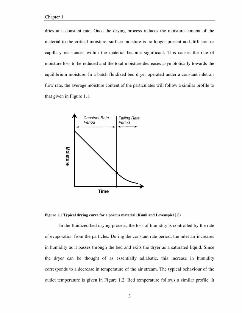
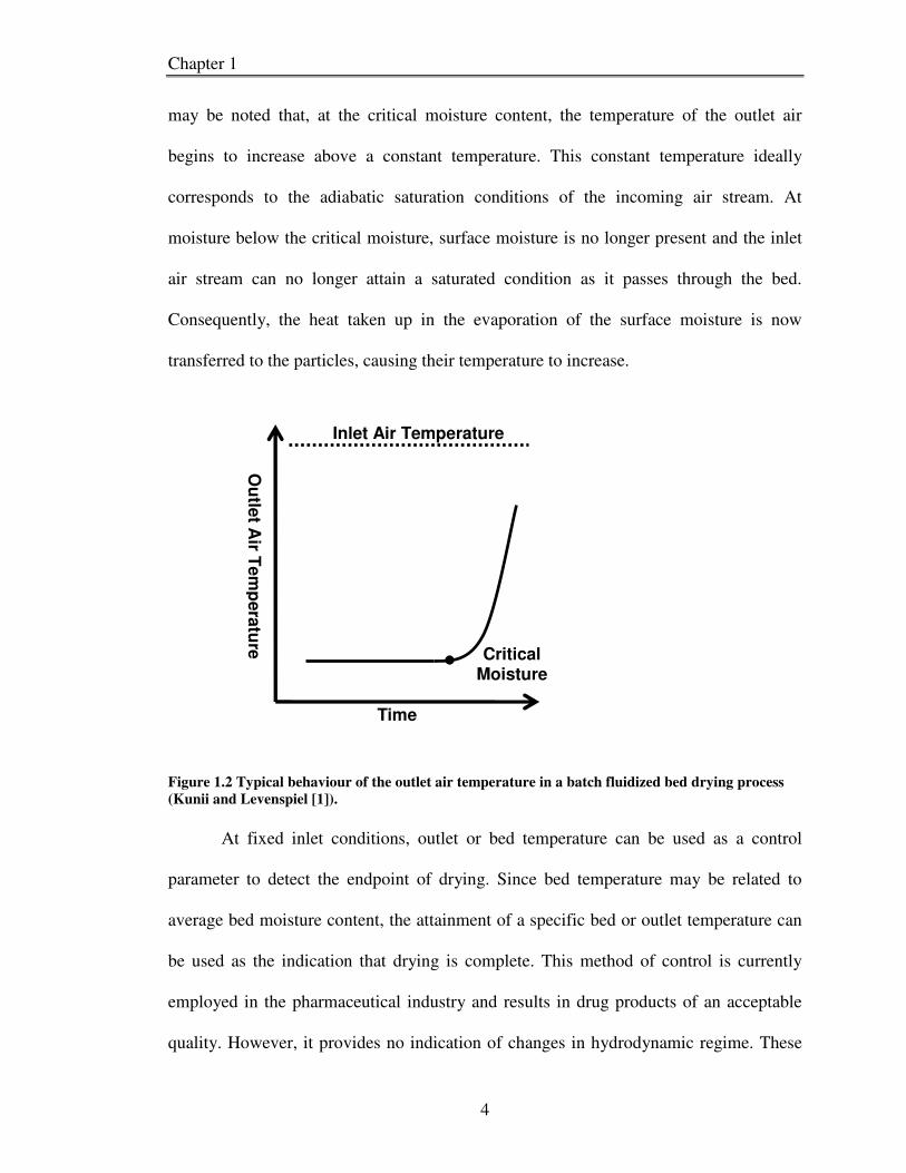

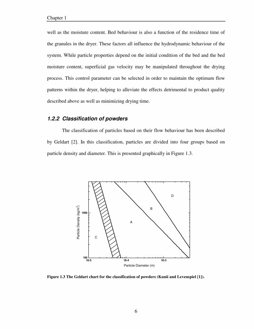


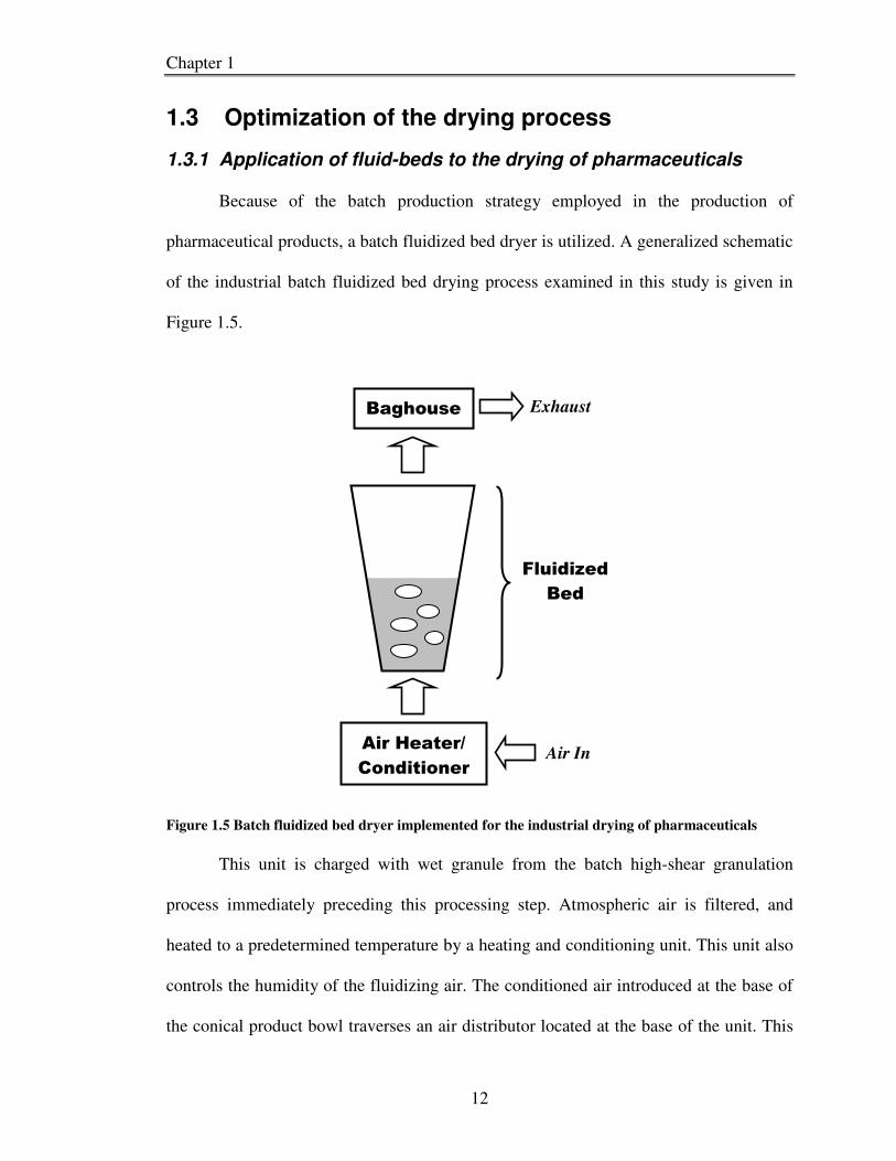


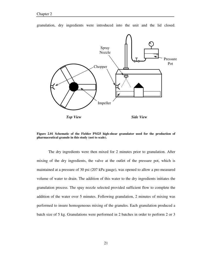

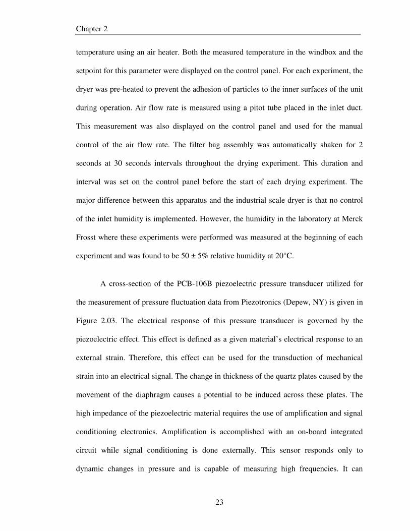


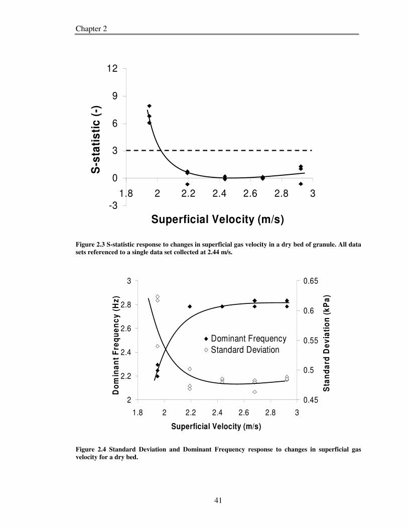


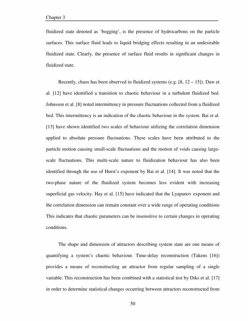


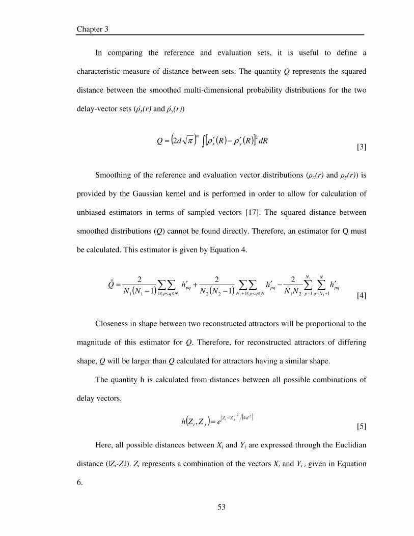


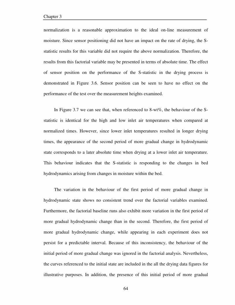
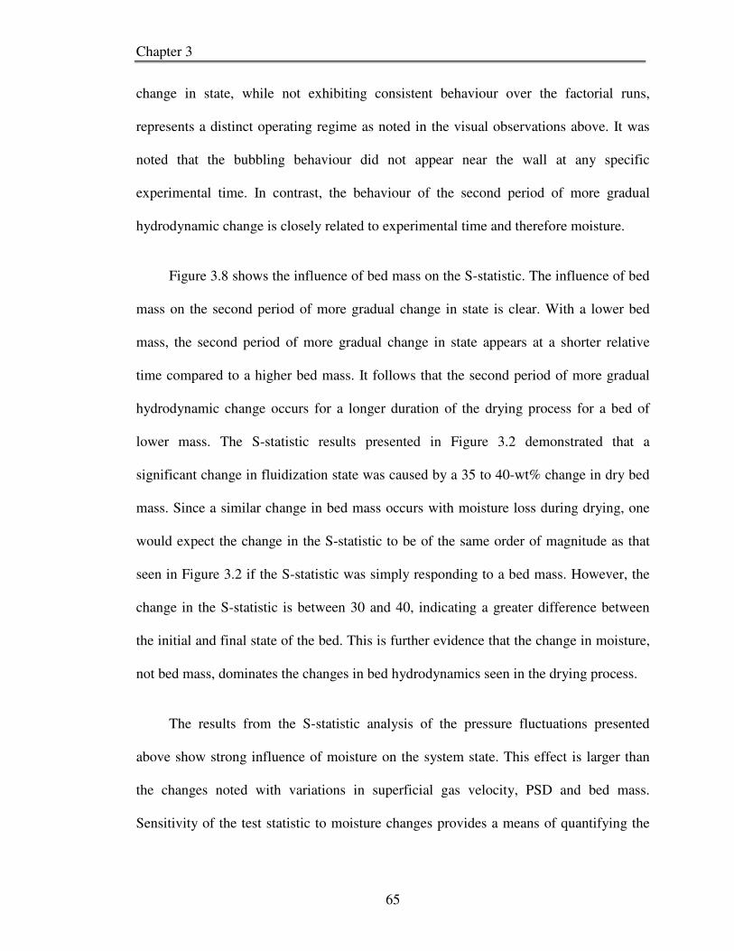


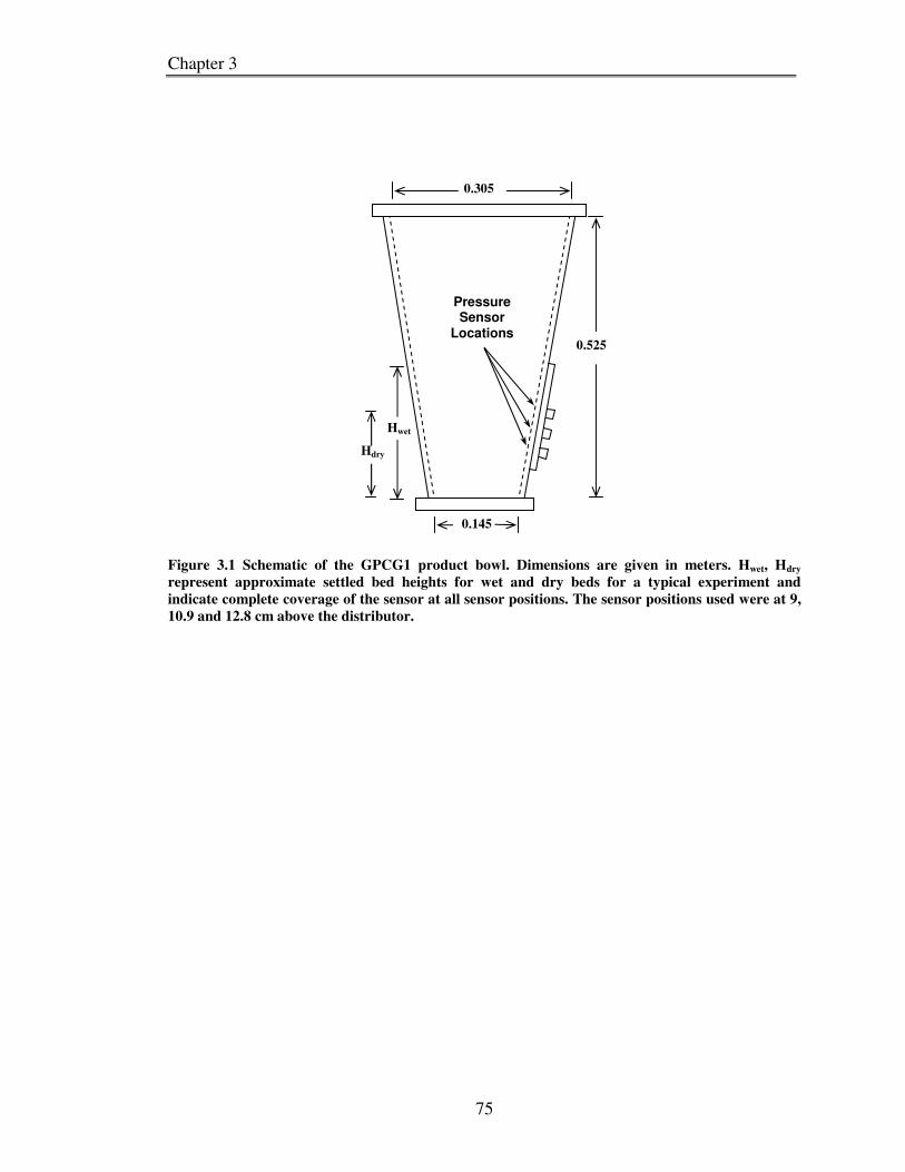
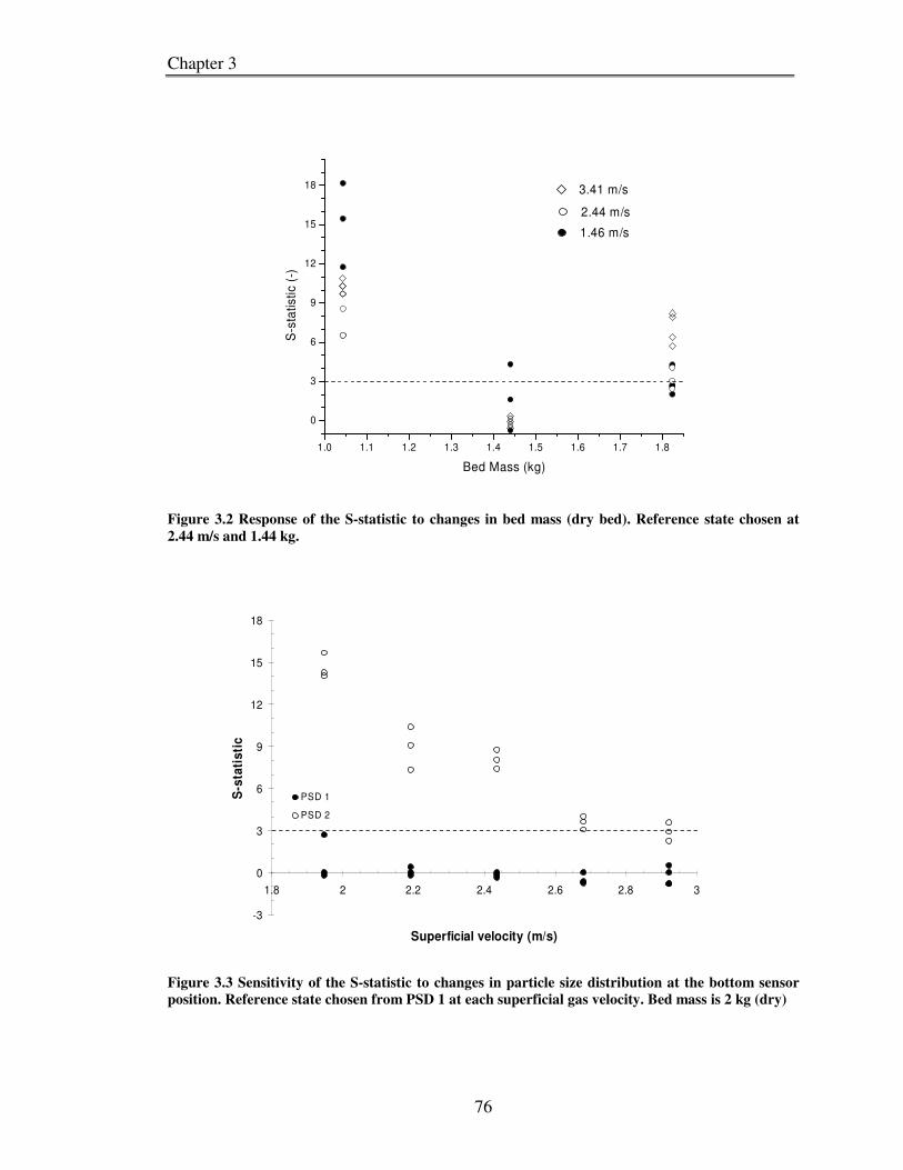


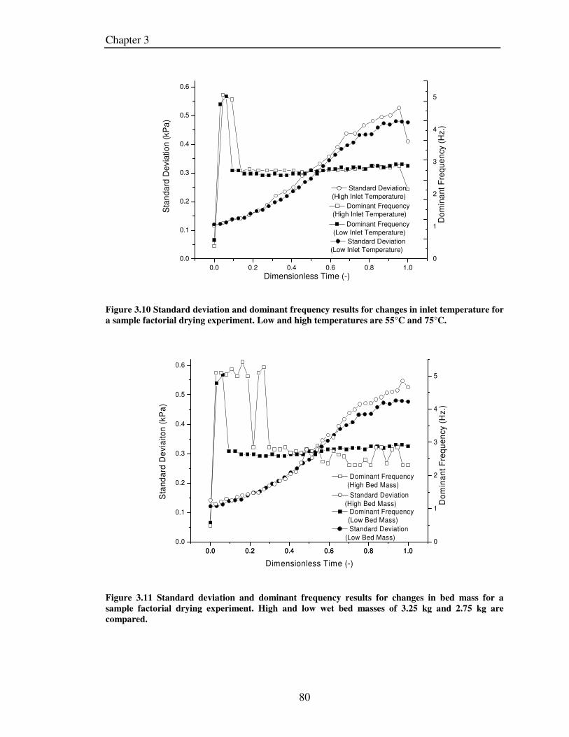


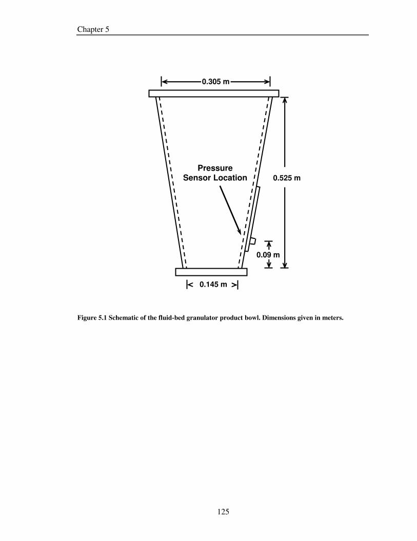


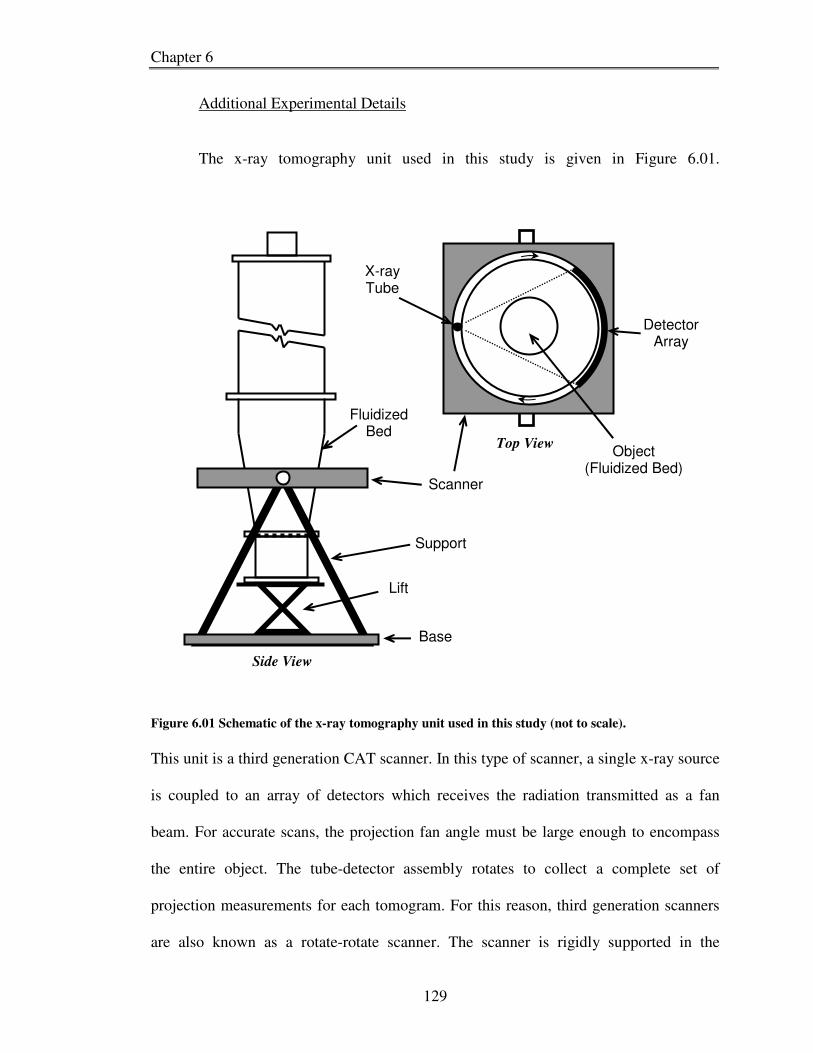


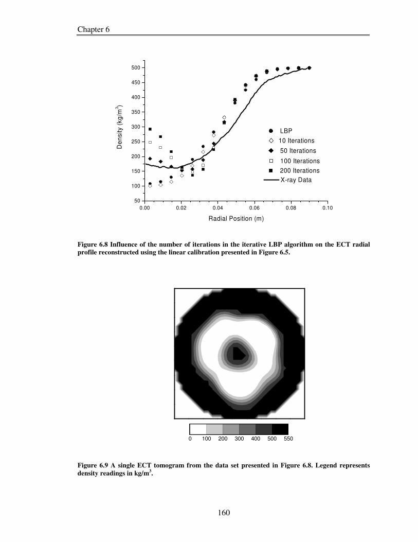
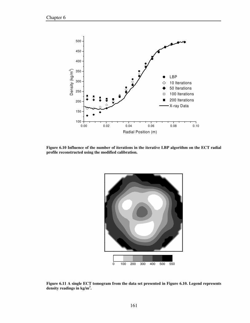


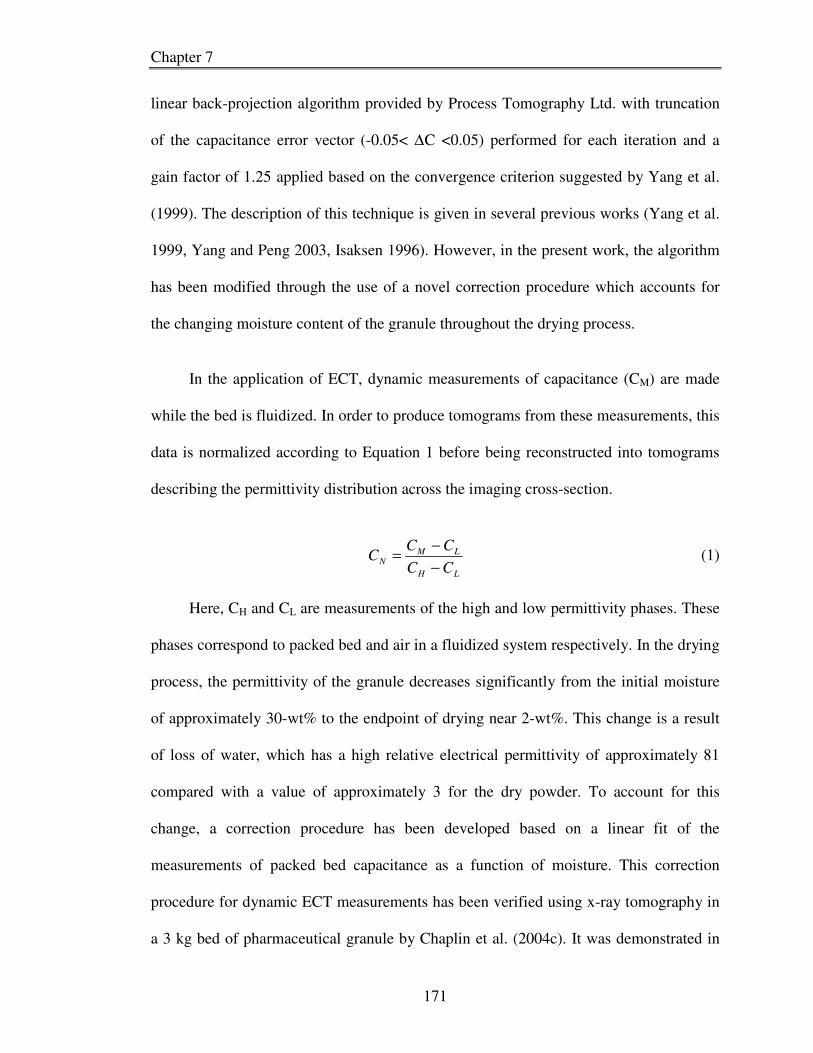


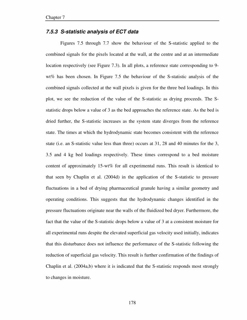


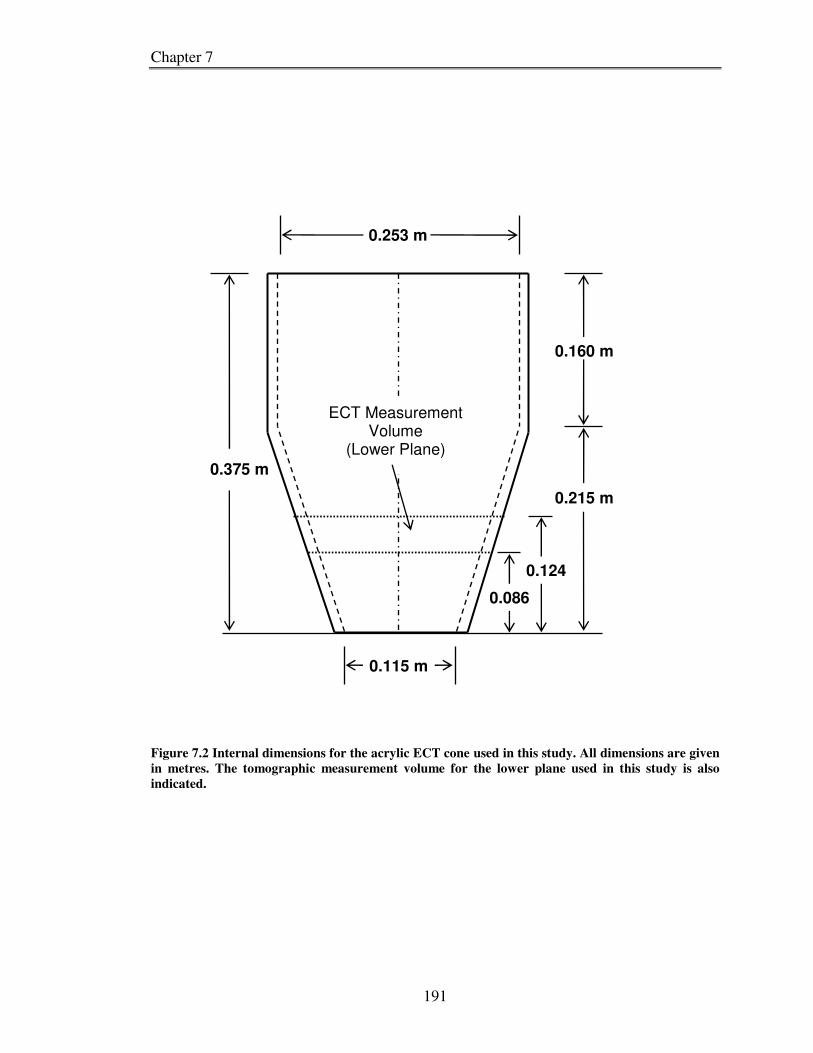


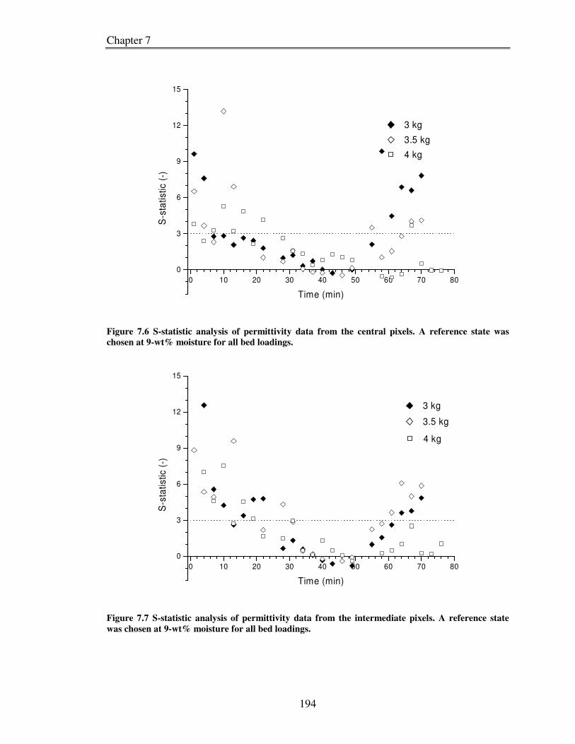
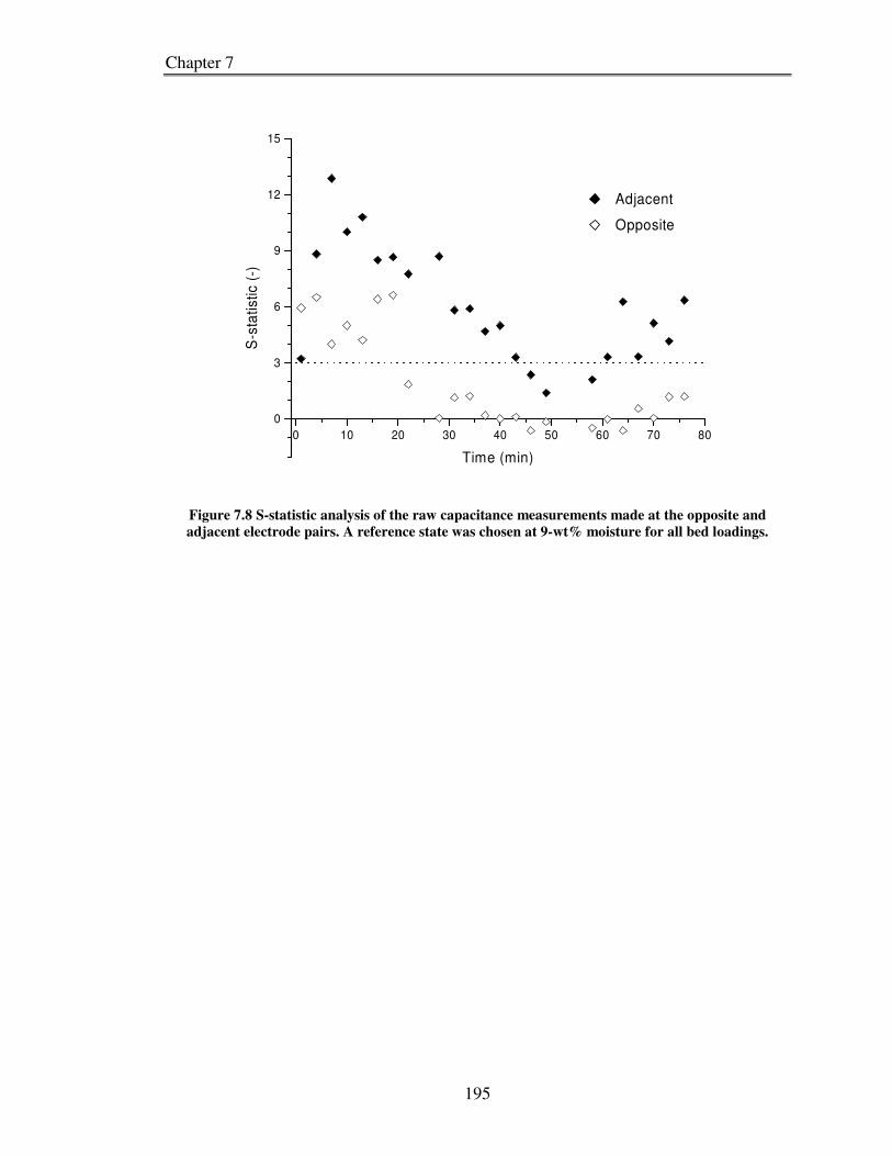


![Poster Programme...[P1.005] Effect of acoustic waves on heat transfer and hydrodynamics characteristics of fluidized bed for binary mixture of ultrafine powder M. Gabhane*1 ,3, S.](https://static.documents.pub/doc/80x56/610376ae949a3d2b8e1a61e3/poster-programme-p1005-effect-of-acoustic-waves-on-heat-transfer-and-hydrodynamics.jpg)


