86


ii Monitoring Manual for Grassland, Shrubland, and Savanna Ecosystems 2nd Edition AdvAncE copy

02/10/16
iMonitoring Manual for Grassland, Shrubland, and Savanna Ecosystems 2nd Edition AdvAncE copy
Monitoring Manualfor Grassland, Shrubland, and Savanna Ecosystems
SECOND EDITION
Volume I: Core Methods
by Jeffrey E. Herrick, Justin W. Van Zee, Sarah. E. McCord, Ericha M. Courtright, Jason W. Karl, and Laura M. Burkett
USDA - ARS Jornada Experimental RangeLas Cruces, New Mexico

ii Monitoring Manual for Grassland, Shrubland, and Savanna Ecosystems 2nd Edition AdvAncE copy
02/10/16
Printed January 2016
Publisher: USDA-ARS Jornada Experimental Range
P.O. Box 30003, MSC 3JER, NMSU Las Cruces, New Mexico 88003-8003
http://jornada.nmsu.edu
ISBN 0-9755552-0-0
Distributed by:
Cover photo: Randy Hayes

02/10/16
iiiMonitoring Manual for Grassland, Shrubland, and Savanna Ecosystems 2nd Edition AdvAncE copy
The monitoring approach and methods described here are the result of a collaboration that began in 1994. The effort was led by the USDA-Agricultural Research Service (ARS) Jornada Experimental Range (JER) in cooperation with the U.S. Environmental Protection Agency (EPA) Office of Research and Development, the Natural Resources Conservation Service (NRCS), and the USDI-Bureau of Land Management (BLM). The development has been guided by suggestions from a large number of indi-viduals who represent landowners, government agen-cies, and environmental organizations in the United States, Mexico, Costa Rica, China, Mongolia, Kenya, Namibia, and Australia. New Mexico State University faculty in particular, have provided ongoing support and input. Funding to support research associated with the development and testing of these protocols has been provided by the USDA-ARS, USDA-NRCS, USDI-BLM, Holloman Air Force Base (AFB), Department of Defense (DoD) Legacy Resources Program, the U.S. EPA, and the National Science Foundation Long-Term Ecological Research program under Grant No. 12-35828. Any opinions, findings, and conclusions or recommendations expressed in this material are those of the author(s) and do not necessarily reflect the views of the National Science Foundation or any of the other organizations listed here. Countless reviewers, work-shop participants, students, and technicians have tested the methods described here. This input has been invaluable.
The manual and specific methods have been improved by suggestions from individuals who rep-
1This list does not necessarily imply endorsement by these organizations.
This is Volume I of a two-part document. Volume II includes guidance on monitoring program design and interpretation, as well as additional methods. For updates, electronic copies of data sheets and a user-friendly Access database and field (touchscreen) data entry system, please visit the USDA-ARS Jornada Experimental Range website (http://jornada.nmsu.edu) and the Landscape Toolbox (http://www.landscapetoolbox.org).
resent the following organizations1:• USDI-BLM
(Alaska, Arizona, Colorado, Idaho, Nevada, New Mexico, Utah, National Operations Center, Washington Office)
• CATIE-Centro Agronómico Tropical de Investigación y Enseñanza (Costa Rica)
• Cattle Growers (New Mexico)• CIAT-Centro de Investigación de Agricultura
Tropical (Honduras) • Conservation Fund (New Mexico)• Department of Defense
(California, New Mexico, Texas)• The Great Basin Institute • INIFAP-Instituto Nacional de Investigaciones
Forestales, Agrícolas y Pecuarias (México)• Land EKG Inc. (Montana)• Mexican Protected Natural Areas
(Chihuahua and Sonora, México)• The Nature Conservancy• Natural Resources Conservation Service
(Arizona, Colorado, Florida, Kansas, Louisiana, New Mexico, Resource Assessment Division)
• New Mexico State University• Peter Sundt Rangeland Consultants• The Quivira Coalition• Synergy Resource Solutions, Inc.• USDA Agricultural Research Service
(Arizona, Colorado, Oregon)• USDA-NRCS Grazing Lands Technology
Institute• USDA-NRCS Soil Quality Institute• USDA-NRCS National Soil Survey Center• U.S. Forest Service (Colorado, New Mexico)• U.S. Geological Survey, Biological Resources
Division (Colorado, Utah)• U.S. National Park Service
(California, Nevada, Utah)
ACKNOWLEDGEMENTS

iv Monitoring Manual for Grassland, Shrubland, and Savanna Ecosystems 2nd Edition AdvAncE copy
02/10/16
BACKGROUND The Core Methods volume of the second edition provides a single, standard reference for the core methods which are part of the BLM Assessment, In-ventory, and Monitoring Strategy (AIM) and NRCS National Resources Inventory (NRI). This contin-ues a process of methods standardization that began in 1998, during the first NRI pilot, continued with the establishment of the NRI on non-federal range-lands in 2003, the publication of the first edition of this manual in 2005, and subsequent adoption of the core methods by the BLM through its national AIM strategy in 2011. The process used to select the core methods for AIM Strategy has been described elsewhere*,**. A similar, but less formal process, was used by the NRCS to select the same methods for the NRI. All of these efforts were stimulated by the 1994 National Academy of Sciences publication, “Rangeland Health”*** and the report by the Soci-ety for Range Management Task Group on Unity in Concepts and Terminology****. Development of this Core Methods volume was also significantly influenced by input from individu-als representing a number of universities, national
* Toevs, G.R., J.W. Karl, J.J. Taylor, C.S. Spurrier, M. Karl, M.R. Bobo, and J.E. Herrick. 2011. Consistent Indicators and Methods and a Scalable Sample Design to Meet Assessment, Inventory, and Monitoring Information Needs Across Scales. Rangelands: 33(4):14-20.
** Herrick, J.E., M.C. Duniway, D.A. Pyke, B.T. Bestelmeyer, S.A. Wills, J.W. Karl and K.M. Havstad. 2012. A Holistic Strategy for Adaptive Land Management. Journal of Soil and Water Conservation 67: 105A-113A.
*** National Research Council. 1994. Rangeland Health: New Ways to Classify, Inventory and Monitor Rangelands. National Academy Press. Washington, DC. 180 pp.
**** Task Group on Unity in Concepts and Terminology Committee Members. 1995. New Concepts for Assessment of Rangeland Condition. Journal of Range Management 48 (3):271–282.
and international organizations, and U.S. federal agencies. The USFS, DoD, and NPS have provided particularly helpful input as we have attempted to align methods with those used by these organiza-tions, where possible, with the view to the eventual development of a national standard. A number of clarifications and minor adjustments were made to the methods to complete the standardization process. Those that have the potential to affect consistency with previously collected data are noted below.
WHAT IS NEW IN THE 2ND EDITION?• The second edition reconciles minor
methodological differences between the first edition, the NRCS NRI program and the BLM AIM Strategy in an effort to further standardize data collection methods among agencies.
• Vegetation height, Species inventory, and Plant identification methods are new additions to Volume I.
• Monitoring program design (Volume II, Chapters 1-8) is amended to reflect the NRCS Conservation Planning Process and the BLM AIM Strategy.
• The Plant density (formerly Belt transect) method is moved from Volume I to the Supplemental Methods section of Volume II.
• Instructions on Establishing a monitoring plot, Plot characterization and Plot observations are enhanced and moved to Volume I.
• New chapters on Quality Assurance and Quality Control are included in Volume I.
• Example transect length is now 25 m (75 ft) but transect length may vary by ecosystem and management objectives.
• Riparian vegetation and channel/gully profile methods are removed from Volume II.
PREFACE TO THE SECOND EDITION

02/10/16
vMonitoring Manual for Grassland, Shrubland, and Savanna Ecosystems 2nd Edition AdvAncE copy
Acknowledgements ........................................................................................................ iii
Preface to the 2nd Edition ...............................................................................................v
Introduction ................................................................................................................... 1
How to Establish a Monitoring Program ....................................................................... 2
How to Establish a Monitoring Plot ............................................................................... 6
Quality Assurance and Quality Control ......................................................................... 9
Plant Identification ...................................................................................................... 14
Plot Characterization ................................................................................................... 16
Plot Observation .......................................................................................................... 23
Core Methods • Photopoints(forvisualrecordofdata) ................................................................. 25 • Line-pointintercept(forcoverandcomposition) ................................................... 27 • Vegetationheight(forverticalstructure) ................................................................ 36 • Gapintercept(forsizeanddistributionofexposedground) ................................... 41 • Soilstabilitytest(forsoilsusceptibilitytowatererosion) ........................................ 47
• Species inventory (for biodiversity) ........................................................................ 55
Data Entry and Quality Control .................................................................................. 58
Appendix A: Plot characterization helpful resources .................................................... 61
Appendix B: Data Sheets .............................................................................................. 63• Equipment Checklist • Plot Checklist• Unknown Plant Tracking Sheet• QA and QC • Plot Characterization• Plot Observation• Photo Points• Line-point Intercept• Line-point Intercept with Height• Vegetation Height• Gap Intercept• Soil Stability• Species Inventory
TABLE OF CONTENTS

02/10/16
1Monitoring Manual for Grassland, Shrubland, and Savanna Ecosystems 2nd Edition AdvAncE copy
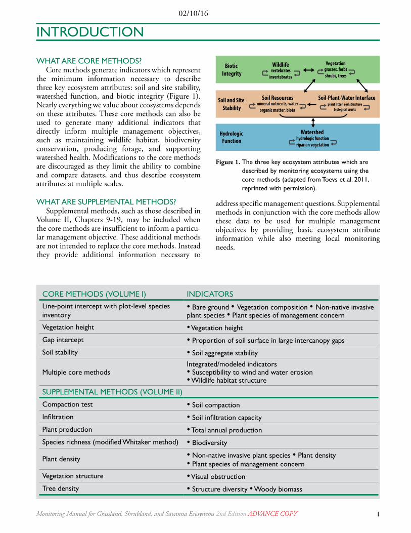
WHAT ARE CORE METHODS?Core methods generate indicators which represent
the minimum information necessary to describe three key ecosystem attributes: soil and site stability, watershed function, and biotic integrity (Figure 1). Nearly everything we value about ecosystems depends on these attributes. These core methods can also be used to generate many additional indicators that directly inform multiple management objectives, such as maintaining wildlife habitat, biodiversity conservation, producing forage, and supporting watershed health. Modifications to the core methods are discouraged as they limit the ability to combine and compare datasets, and thus describe ecosystem attributes at multiple scales.
WHAT ARE SUPPLEMENTAL METHODS?Supplemental methods, such as those described in
Volume II, Chapters 9-19, may be included when the core methods are insufficient to inform a particu-lar management objective. These additional methods are not intended to replace the core methods. Instead they provide additional information necessary to
address specific management questions. Supplemental methods in conjunction with the core methods allow these data to be used for multiple management objectives by providing basic ecosystem attribute information while also meeting local monitoring needs.
Figure 1. The three key ecosystem attributes which are described by monitoring ecosystems using the core methods (adapted from Toevs et al. 2011, reprinted with permission).
CORE METHODS (VOLUME I) INDICATORSLine-point intercept with plot-level species inventory
• Bare ground • Vegetation composition • Non-native invasive plant species • Plant species of management concern
Vegetation height • Vegetation height
Gap intercept • Proportion of soil surface in large intercanopy gaps
Soil stability • Soil aggregate stability
Multiple core methodsIntegrated/modeled indicators• Susceptibility to wind and water erosion • Wildlife habitat structure
SUPPLEMENTAL METHODS (VOLUME II)Compaction test • Soil compaction
Infiltration • Soil infiltration capacity
Plant production • Total annual production
Species richness (modified Whitaker method) • Biodiversity
Plant density • Non-native invasive plant species • Plant density • Plant species of management concern
Vegetation structure • Visual obstruction
Tree density • Structure diversity • Woody biomass
Biotic Integrity
Hydrologic Function
Soil and Site Stability
Vegetationgrasses, forbs shrubs, trees
Wildlifevertebrates
invertebrates
Soil Resourcesmineral nutrients, water
organic matter, biota
Soil-Plant-Water Interfaceplant litter, soil structure
biological crusts
Watershedhydrologic functionriparian vegetation
Soil Resources
INTRODUCTION

2 Monitoring Manual for Grassland, Shrubland, and Savanna Ecosystems 2nd Edition AdvAncE copy
02/10/16
Figure 2. Field monitoring measurement using Line-point intercept in Mongolia.
Core Methods is the only volume needed if all of the following are “true.”
CRITERIA TRUE FALSEIF FALSE,
THEN SEE VOLUME II
My management objectives are fairly well described. Chapter 1
I already know where I want to monitor. Chapter 3
I already know how frequently I want to monitor. Chapter 4
The core indicators will answer my monitoring questions. Chapter 4
The basic monitoring strategy sounds reasonable, and I am either not aware of compaction or other problems not covered by the core methods or I have decided not to monitor these problems.
Chapter 4
I am comfortable with a standard number of measurements (page 5) that will allow me to document large changes but may miss smaller changes.
Chapter 4
I am not planning to monitor riparian areas. Chapter 22
I already know how to interpret the indicators. Chapter 21*
* For information about how to calculate additional indicators and interpret your results, please see Volume II, Chapters 20 and 21.
IS THE CORE METHODS VOLUME ALL I NEED?
Before collecting field monitoring measurements (Figure 2) it is important to specify why, where, how, at what frequency, and at what intensity you will monitor. The methods described in the Core Methods volume are part of Step 8 in implementing a moni-toring program (Figure 3). Describing the anticipat-ed data analysis and interpretation of the monitoring data will also inform the characteristics of the moni-toring program design. Volume II of this manual provides detailed guidance on monitoring program design, data analysis and interpretation. In some cases, you may need to refer to Volume II (see ques-tions below) before continuing to read the rest of the Core Methods volume.
HOW TO ESTABLISH A MONITORING PROGRAM

02/10/16
3Monitoring Manual for Grassland, Shrubland, and Savanna Ecosystems 2nd Edition AdvAncE copy
Figure 3. Monitoring of core indicators program design, implementation and integration with management. For more detail on monitoring program design, see Volume II, Chapters 1-8.
Step 10: Document management and disturbance; record short-term monitoring data (if applicable)
Step 11: Repeat monitoring at pre-determined frequency and perform data QA & QC
Step 12: Analyze, interpret, report, and use monitoring results to apply adaptive management
First Year: Develop Monitoring Program
First Year: Implement Monitoring Program
Every Year:Maintain Program
Every 1-10 Years*: Repeat Long-term Monitoring
Step 4: a) Select and document supplemental monitoring methods; b) estimate sample sizes; c) set sampling frequency; d) develop implementation rules
Step 8: Establish monitoring locations; collect data and perform QA; perform data QC
Step 9: Evaluate baseline data and re�ne monitoring design and monitoring objectives as necessary
*The frequency of repeat monitoring will vary by management objective. Typically, treatments (e.g., riparian restoration, post-�re rehabilitation) involving relatively rapid responses or where more frequent data may inform adaptive management (e.g., management changes in more mesic environments) require monitoring frequencies of less than once every 5 years. For more long-term management objectives (e.g., grazing management) and in arid environments where responses to management changes are slow to occur, monitoring frequencies of 8-10 years are usually su�cient.
Step 6: Apply strati�cation and select statistically valid monitoring locations
Step 5: Collect and evaluate pilot data to determine sampling su�ciency and the validity of the strata
Step 7: Develop QA & QC procedures and data management plans
Step 1: Develop management objectives; select additional ecosystem attributes & indicators to monitor
Step 2: Set the study area and reporting units; develop monitoring objectives
Step 3: Select criteria for stratifying study area into similar land areas (if required).
First Year: Design Monitoring Program
How to Establish a Monitoring Program

4 Monitoring Manual for Grassland, Shrubland, and Savanna Ecosystems 2nd Edition AdvAncE copy
02/10/16
MEMBERS OF A MONITORING TEAM (ONE INDIVIDUAL MAy HAVE MULTIPLE ROLES)
ROLE RESPONSIBILITy
Land Manager
• Develop management objectives and questions• Develop monitoring objectives• Select supplemental indicators to be monitored• Determine area to be monitored• Design project specifications• Select supplemental methods• Describe QA and QC protocols• Interpret results
Field Crew Leader
• Oversee crew training and calibration• Coordinate data collection• Record data in electronic database or onto paper data sheets• Ensure QA on each data sheet• Coordinate QC on each data sheet
Recorder • Record data in electronic database or onto paper data sheets• Perform QA on each data sheets
Observer • Perform data collection method• Ensure proper technique for each method
Data Entry • Enter data from paper data sheets into a digital format (e.g., Access database, Excel spreadsheet)
Data Error Checking • Check transcription from paper data sheets to digital format• Perform QC on each data sheet
QUICK START MONITORING PROGRAM CHECKLIST*
STEP DONE?
Define monitoring objectives.
Review the adequacy of the core indicators and add supplemental or contingent indicators as needed.
Assemble background information (maps, photos, management history) and select general areas you would like to monitor.
Select monitoring sites. This may involve preliminary evaluations of risk or opportunity for change.
Define quality assurance and quality control objectives.
Describe each monitoring site’s management, landscape, and soil characteristics.
Establish permanent transects and begin monitoring.
* For a more detailed checklist, see the Introduction of Volume II, Section I.
How to Establish a Monitoring Program
02/10/16
5Monitoring Manual for Grassland, Shrubland, and Savanna Ecosystems 2nd Edition AdvAncE copy
Photos Canopy and basal gap interceptLine-point intercept Soil stability test
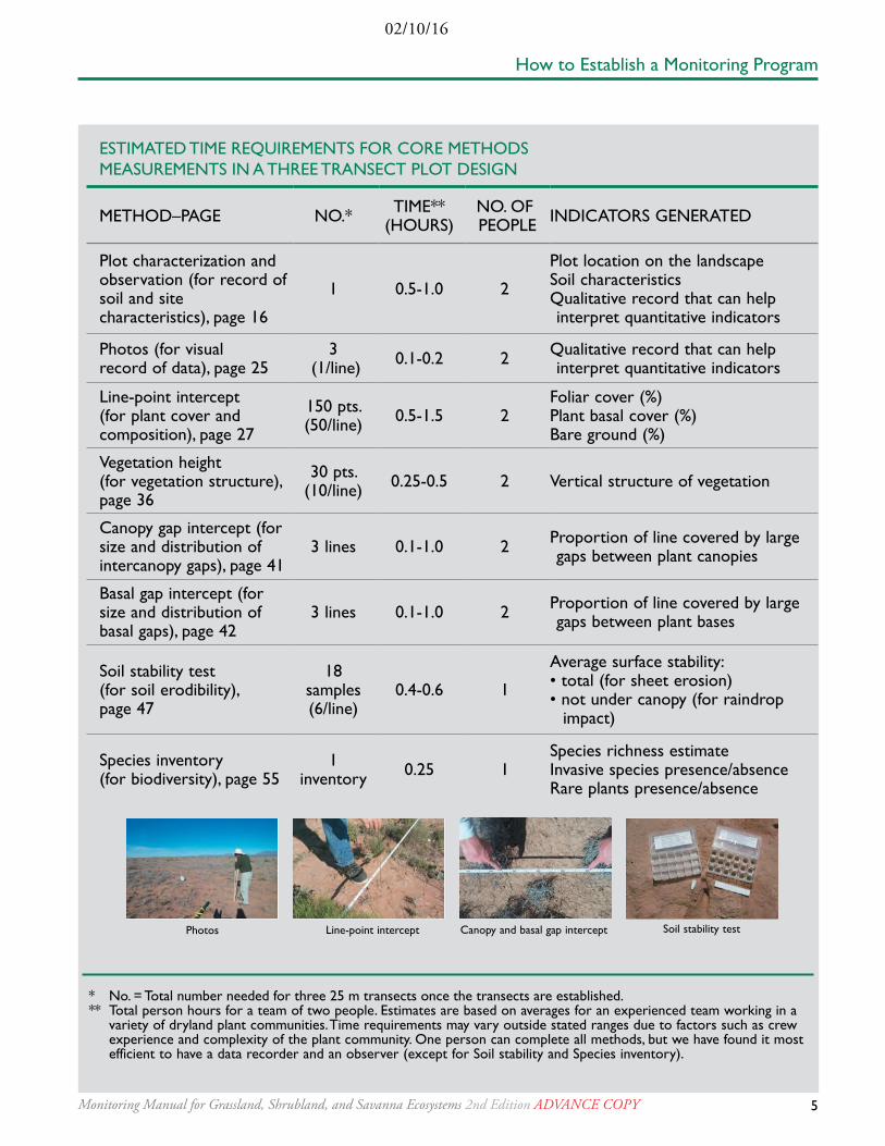
* No. = Total number needed for three 25 m transects once the transects are established.** Total person hours for a team of two people. Estimates are based on averages for an experienced team working in a
variety of dryland plant communities. Time requirements may vary outside stated ranges due to factors such as crew experience and complexity of the plant community. One person can complete all methods, but we have found it most efficient to have a data recorder and an observer (except for Soil stability and Species inventory).
ESTIMATED TIME REQUIREMENTS FOR CORE METHODS MEASUREMENTS IN A THREE TRANSECT PLOT DESIGN
METHOD–PAGE NO.* TIME** (HOURS)
NO. OF PEOPLE INDICATORS GENERATED
Plot characterization and observation (for record of soil and site characteristics), page 16
1 0.5-1.0 2
Plot location on the landscapeSoil characteristicsQualitative record that can help interpret quantitative indicators
Photos (for visual record of data), page 25
3 (1/line) 0.1-0.2 2 Qualitative record that can help
interpret quantitative indicators
Line-point intercept (for plant cover and composition), page 27
150 pts.(50/line) 0.5-1.5 2
Foliar cover (%) Plant basal cover (%)Bare ground (%)
Vegetation height (for vegetation structure), page 36
30 pts. (10/line) 0.25-0.5 2 Vertical structure of vegetation
Canopy gap intercept (for size and distribution of intercanopy gaps), page 41
3 lines 0.1-1.0 2 Proportion of line covered by large gaps between plant canopies
Basal gap intercept (for size and distribution of basal gaps), page 42
3 lines 0.1-1.0 2 Proportion of line covered by large gaps between plant bases
Soil stability test (for soil erodibility), page 47
18 samples(6/line)
0.4-0.6 1
Average surface stability: • total (for sheet erosion)• not under canopy (for raindrop
impact)
Species inventory(for biodiversity), page 55
1 inventory 0.25 1
Species richness estimateInvasive species presence/absenceRare plants presence/absence
How to Establish a Monitoring Program
6 Monitoring Manual for Grassland, Shrubland, and Savanna Ecosystems 2nd Edition AdvAncE copy
02/10/16
It is important to carefully locate and describe each monitoring plot for two reasons. First, this information enables comparison of data collected on plots with similar soils, topography and climate – all of the which determine site potential. Second, this information helps to relocate the plot to continue monitoring that location over time.
ESTABLISH AND PERMANENTLy MARK PLOTS AND TRANSECTS
Before establishing the plot, verify that the site is suitable by checking it against the “rejection criteria” listed on the Monitoring Program Design Form I (Volume II, Chapter 1). Strict adherence to the rejec-tion criteria protocol is necessary to preserve the population monitored and to eliminate bias.
Permanent plot and transect markers such as rebar stakes or rock cairns can be installed to assist with plot relocation. Do not use t-posts, which can be attractive to livestock and wildlife, which rub against them. In projects where permanent markers are not permitted, such as in the NRI, precise GPS coordi-nates alone will suffice. For more information on plot monumentation, see Elzinga et al. 2001*.
It is recommended that more than one transect be established at a plot. Multiple transects distribute observations across the plot, capture within-plot vari-ability, and are less sensitive to directional patterns than a single transect. Transect length may vary by project, but should be applied consistently at each plot. See Volume II for a more information on mod-ifying transect length and other plot measurements.
* Elzinga, C.L., D.W. Salzer, J.W. Willoughby and J.P. Gibbs. 2001. Monitoring Plant and Animal Populations, Blackwell Publishing. 368 pp.
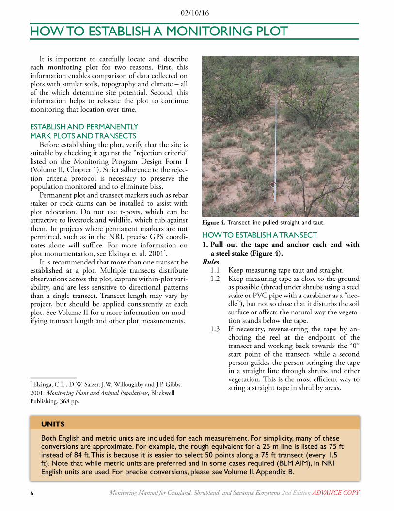
HOW TO ESTABLISH A TRANSECT1. Pull out the tape and anchor each end with
a steel stake (Figure 4).Rules
1.1 Keep measuring tape taut and straight.1.2 Keep measuring tape as close to the ground
as possible (thread under shrubs using a steel stake or PVC pipe with a carabiner as a “nee-dle”), but not so close that it disturbs the soil surface or affects the natural way the vegeta-tion stands below the tape.
1.3 If necessary, reverse-string the tape by an-choring the reel at the endpoint of the transect and working back towards the “0” start point of the transect, while a second person guides the person stringing the tape in a straight line through shrubs and other vegetation. This is the most efficient way to string a straight tape in shrubby areas.
Figure 4. Transect line pulled straight and taut.
Units
Both English and metric units are included for each measurement. For simplicity, many of these conversions are approximate. For example, the rough equivalent for a 25 m line is listed as 75 ft instead of 84 ft. This is because it is easier to select 50 points along a 75 ft transect (every 1.5 ft). Note that while metric units are preferred and in some cases required (BLM AIM), in NRI English units are used. For precise conversions, please see Volume II, Appendix B.
HOW TO ESTABLISH A MONITORING PLOT

02/10/16
7Monitoring Manual for Grassland, Shrubland, and Savanna Ecosystems 2nd Edition AdvAncE copy
MULTIPLE TRANSECT PLOT DESIGNS2. Spoke design (Figure 5a).Rules
2.1 Place a permanent stake into the ground at the center of the monitoring plot. This stake will also serve as the camera point (Photo Points, page 25).
2.2 Starting with 0 degrees or a randomly select-ed azimuth (compass direction: 0° to 359°), extend a tape in the azimuth direction to a distance of 5 m (15 ft) further than the length of the transect. Install a stake at the 5 m mark. This will serve as the 0 m end of your transect, because the transect begins 5 m from the center point.
2.3 Anchor the far end of the transect with a stake.
Repeat transect establishment at regular intervals in a circle around the plot. The in-terval depends on the number of transects. Many monitoring programs use three tran-sects, with 120° between each transect.
3. Intersecting transect design (NRI) (Figure 5b).Rules
3.1 For instructions on establishing an NRI in-tersecting transect plot, see the NRI Graz-ing Land On-Site Data Collection Hand-book of Instructions (http://www.nrisurvey.org/nrcs/Grazingland/2015/instructions/instruction.htm). The NRI instructions are updated annually. Substitute “2015” for the current year when visiting this handbook.
3.2 Two 50 m (150 ft) transects are laid out per-pendicular to each other. The tapes should intersect at the 25 m (75 ft) mark (see the Plot Design box).
3.3 Be careful to minimize trampling inside the plot, as the plot center is also part of the data collection area.
3.4 When collecting Line-point intercept mea-surements on a crossed-transect design, make sure that the point at 25 m (75 ft), where the transects meet, is only included once in indicator calculations.
4. Parallel transect design (Figure 5c).Rules
4.1 Identify the azimuth of the slope or a ran-domly selected azimuth.
4.2 Extend the tape in the azimuth direction to establish a base transect.
4.3 Systematically place transects perpendicular to the base transect.
4.4 Anchor both ends of each transect with a stake.
SINGLE TRANSECT PLOT DESIGNS5. Single transect upland design (Figure 5d).Rules
5.1 Anchor and mark the 0 m end of the tran-sect.
5.2 Using a randomly selected azimuth (compass direction: 0° to 359°), extend the tape in the azimuth direction to establish the transect.
5.3 Anchor the far end of the transect with a stake.
6. Single transect linear feature (e.g., stream, pipe-line, road) design (Figure 5e).
Rules6.1 Anchor and mark the 0 m end of the tran-
sect. Ensure the 0 m end is placed such that the transect will cross the linear feature per-pendicular to the feature, and the 0 m end is 5 m beyond the feature.
6.2 Extend the tape perpendicular to the linear feature.
6.3 Anchor the far end of the transect with a stake.
How to Establish a Monitoring Plot

8 Monitoring Manual for Grassland, Shrubland, and Savanna Ecosystems 2nd Edition AdvAncE copy
02/10/16
PLOT LAyOUT DESCRIPTION
(a) Spoke Design
25 m spoke design covers ~0.3-hectare (~0.7 acres). 50 m (~75 ft) spoke design covers a 1 hectare (~2.35 acres) area. Transects begin 5 m (15 ft) from the plot’s center to focus trampling around center stake and minimize disturbance effects on transects.
(b) Intersecting Design
The NRI intersecting transect design covers ~0.2 hectares (~0.4 acres). Two 50 m (150 ft) transects intersect at the 25 m (75 ft) mark at plot center. The transect arms are oriented 45 degrees in both directions from magnetic north.
(c) Parallel Transect Design
Standard transect length is 25 m (75 ft). Parallel transects are evenly spaced. Transects may run perpendicular to the slope or perpendicular to a randomly selected azimuth.
(d) Single Transect Design
Standard transect length is 25 m (75 ft); a multiple single transect design is often used to maximize replication at landscape scale.
(e) Linear Feature Design
(e.g., riparian)
Standard transect length is 25 m (75 ft); a multiple single transect design is often used to maximize replication at landscape scale. Length may vary depending on linear feature size, extent, or potential impact.
QUALitY AssURAnCE
☐ Avoid disturbing vegetation and the soil surface in the transect area. ☐ Keep the transect tape as close to the ground as possible by threading the tape under vegetation yet do not disturb the soil surface while doing so.
☐ If needed, use additional stakes at various intervals to secure the tape close to the ground, especially where wind is a consideration.
☐ GPS coordinates for the plot location and transect start points (where required) are recorded on the Plot Characterization Data Sheet.
☐ Always walk on the same side of the transect tape.
How to Establish Monitoring Plots
Figure 5. Example plot layout designs. Plot layouts may be adjusted to meet monitoring objectives so long as the number of measurements taken remains the same.

02/10/16
9Monitoring Manual for Grassland, Shrubland, and Savanna Ecosystems 2nd Edition AdvAncE copy
The power of monitoring data cannot be over-stated. As data are applied to land management deci-sions and research questions, the utility of the data are amplified. A data error in the field can be com-pounded as analysis and interpretation of the data progresses, and can ultimately affect results and con-clusions. Conversely, high quality data will be strengthened by strict adherence to protocols and procedures to minimize sampling error. For this rea-son, correct and consistent technique among field observers and careful attention of data recorders is critical. A carefully planned sequence of quality assurance and quality control steps will ensure the integrity and accuracy of the data.
TyPES OF ERROR IN MONITORINGSeveral types of data errors can occur in a moni-
toring project. Sampling error occurs when your estimate of an indicator is different than the actual (true) value because you have sampled only a portion of the entire population. Good sample design (see Volume II, Chapter 5) ensures that sampling errors only affect the precision of the estimate without affecting its accuracy (i.e., no bias). Good sample design also allows you to calculate and minimize sampling error. Measurement error is a type of non-
sampling error that occurs when the value recorded is different than the true value for an object being observed. This could be because the object was mea-sured incorrectly by the observer or because the object was recorded incorrectly by the data recorder. Measurement errors can affect both precision and accuracy, resulting in biased results. This section dis-cusses minimizing measurement errors in monitoring data.
WHAT ARE QA AND QC?Quality assurance (QA) and quality control (QC)
are processes of ensuring data integrity and minimiz-ing measurement errors throughout the monitoring process, from planning your monitoring objectives to data collection to data analysis and interpretation.
Quality assurance is a proactive process employed to maintain data integrity. Training, calibration, proper technique, standardized data organization, on-plot data review, readjustments in response to data review, and communication between the data manager and data gatherers are all components of quality assurance. Quality assurance is a continuous effort to prevent, detect, and correct measurement errors throughout the monitoring project.
Quality control is a reactive process to detect mea-surement errors after the data collection process is complete. Quality control will also determine com-pliance with applicable standards and can be project or protocol specific. Users of monitoring data pre-determine the amount of variability or error they are willing to accept for certain measurements. A prop-erly designed QC protocol describes the level of error in a data set. Defects detected in the data set are often resolved by deleting data that are not suitable for analysis. Data corrections or replacements are rare and must be substantiated by other data sources. Good habits in QA will minimize the effort and data deletion associated with QC.
WHERE DO QA AND QC OCCUR?Quality assurance takes place in a unique way at
nearly every step of the project: planning, training, calibration, data collection, data compilation, and data review.
Quality control takes place in the office or at a time and place removed from the data collection event.
QUALITy ASSURANCE AND QUALITy CONTROL
Figure 6. Careful establishment of a plot is one step in the quality assurance process.

10 Monitoring Manual for Grassland, Shrubland, and Savanna Ecosystems 2nd Edition AdvAncE copy
02/10/16
WHEN DO QA AND QC OCCUR?Quality assurance is an all-encompassing process
from the beginning of the monitoring project until its conclusion. Daily QA to clean data and correct technique takes place in the field. Errors detected during QA are corrected immediately as you are in the same time and place as the actual plot conditions.
Quality control occurs after all field decisions (good and bad) have taken place. Error corrections during QC are limited because plots cannot be revis-ited with the exact conditions that occurred during data collection.
WHO IS RESPONSIBLE FOR QA AND QC?Everyone involved in a monitoring project is
responsible for a portion of QA and QC (see page 4). The land manager provides clear communication of the monitoring objectives and methods so that data are collected appropriately. The land manager pro-vides expert-level training and support, organization, calibration and justification of personnel expertise, field observer oversight, and quality control checks.
Since QC is an inspecting/checking process, it can be performed by anyone, as long as they know the limits and parameters of the data they are checking. Sometimes a brief training session is necessary for QC personnel, so they know how to identify errors. Once identified, the data manager makes the deci-sion what to do next. If an error is unexplainable, this is called nonconformity, and the data are deleted. Occasionally, an investigation can help decipher an error, and the data can be retained.
Data recorders and observers are in the most pow-erful position to ensure data integrity, as they are the plot experts. It is the role of the field team to record an accurate portrayal of the plot for the land man-ager. A well-defined QA plan is the most effective way for the data gatherer to ensure the data set is utilized to its potential.
ARE QA AND QC REQUIRED?Yes. QA and QC are an integral part of monitor-
ing to ensure data consistency and accuracy.
QUALITy ASSURANCE ACTIVITIES THROUGHOUT THE DATA COLLECTION PROCESSFREQUENCy ACTIVITy
Continuously
• Practice proper technique.• Maintain data organization.• Document errors.• Keep the ecological context in mind.• Solicit expert advice if needed. • Back up your data.
Daily
• Review data sheets for completeness and correctness. If errors are found, return to the plot to collect the correct data.
• Upload and name photos.• Identify unknown plant species. • Back up your data after corrections have been made.
Weekly
• Review data for completeness and errors with an ecosystem expert or team leader.
• Identify any remaining unknown plant species. • Back up your data.
Monthly ANDupon change to a new ecosystem
• Calibrate data gatherers for each method in the protocol.• Review data for completeness and errors with an
ecosystem expert or team leader. • Back up your data.
Quality Assurance and Quality Control
02/10/16
11Monitoring Manual for Grassland, Shrubland, and Savanna Ecosystems 2nd Edition AdvAncE copy
ARE QA AND QC THE SAME FOR EACH METHOD AND PROJECT?
No. The general principles of QA and QC apply throughout the project, but practical QA activities will vary by method. For each method in this manual, quality assurance methods are also explained. See page 57 for a description of QC procedures in more detail.
STANDARD METHODS (RULE SET)1. Begin project metadata (see Volume II). Rules
1.1 Define monitoring objectives and project area.
1.2 Determine indicators and appropriate data collection methods.
1.3 Document sample design. 1.4 Determine the acceptable range of error for
data collection. This includes the maximum range of variation permissible in the GPS coordinates and crew calibration.
1.5 Determine plot rejection criteria.1.6 Describe project plot layout. Be sure to doc-
ument the required number, length, and lo-cation of transects within the plot.
2. Provide training to field data collection crews.Rules
2.1 Train crews in the appropriate data collec-tion methods as described in this manual and developed in Step 1.
2.2 Use expert trainers and online method videos (http://www.landscapetoolbox.org) to provide consistent and correct training.
2.3 Provide QA procedure training to all field crews.
3. Calibrate all field crews. Rules
3.1 Lay out a measuring tape exactly as you would for a monitoring transect.
3.2 Select an area with a diverse assortment of features that will represent the ecosystem being monitored. Consider the vegetation diversity, soil surface features, and heteroge-neity.
3.3 Each observer collects data along the same transect, following the method rules and QA for each method.
3.4 Be especially careful not to move the transect tape for these exercises. An immobile tape will help reflect the data gatherer's effort, rather than variability due to a moving tape.
3.5 Encourage data gatherers to step lightly around the transect tape, otherwise the area around it will be heavily trampled.
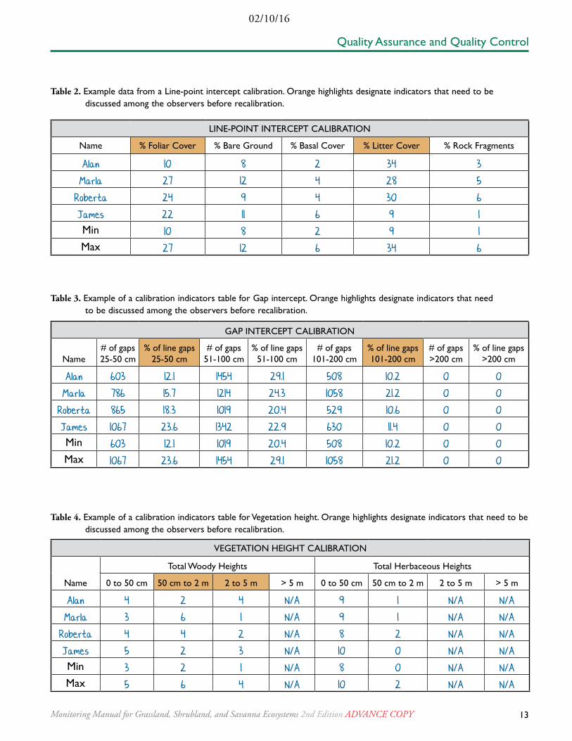
3.6 Calculate the indicator summaries. It may be helpful to record results into a table (e.g., Tables 2, 3, and 4).
3.7 Assess the range of variation among data gatherers (Table 1). Is it acceptable?
3.8 If data gatherers are not within the accept-able range of variation, examine the data sheets to identify where discrepancies oc-cur. Walk the transect as a group and note unique and problematic features along the line. Discuss the methodology, quality assur-ance rules and repeat Steps 3.3-3.7.
Quality Assurance and Quality Control
CALiBRAtiOn
Calibration of data gatherers is an integral component of the quality assurance process. Calibration ensures that a data gatherer collects data accurately each time and that data are collected consistently with other data gatherers, including the training expert. Calibration of all data gatherers occurs immediately following training, each time data collection begins in a new ecosystem, and at regular intervals throughout the monitoring season. During each calibration, the expert data collector or trainer observes each data gatherer for proper technique and corrects methodological problems immediately.

12 Monitoring Manual for Grassland, Shrubland, and Savanna Ecosystems 2nd Edition AdvAncE copy
02/10/16
METHOD CALIBRATION CRITERIA
Line-point intercept
Gap intercept
All observers must be within 10% absolute of one another for each indicator. For example, if calculated indicators are 23%, 24.5%, 30.5%, and 32%, then calibration criteria have been met. However if calculated indicators are 89%, 79%, 84%, and 90%, then calibration criteria have not been met.
Vegetation height Count the number of vegetation heights in each category. The number of plant heights in each category should not differ by more than 2.
Species inventory The number of species recorded by each observer should differ by no more than 2 species
Table 1. Calibration criteria for each field method that can be calibrated.
Quality Assurance and Quality Control
4. Begin data collection. Rules
4.1 Follow data collection methods completely and consistently.
4.2 Review data sheets for completeness and correctness. If errors are identified, return to the plot to collect the correct data.
4.3 Back up your data early and often.
5. Recalibrate field crew.Rules
5.1 Recalibrate crews once per month or upon transitioning to data collection in a new eco-system, whichever comes first.
5.2 Follow calibration methods described in Step 3.
6. Archive calibration data.
7. Complete data collection.
8. Review data for completeness and correctness. If errors are identified, return to the plot to collect the correct data.
9. If data were collected on paper data sheets, enter data into a digital format (e.g., Access database or Excel spreadsheets). See page 58 for data entry methods.
10. Conduct QC, page 58.
11. Complete project metadata.Rules
11.1 Note which plots were sampled. 11.2 Note which plots were visited but rejected,
and list the reason(s) for plot rejections. 11.3 Note which plots were never visited.
02/10/16
13Monitoring Manual for Grassland, Shrubland, and Savanna Ecosystems 2nd Edition AdvAncE copy
LINE-POINT INTERCEPT CALIBRATION
Name % Foliar Cover % Bare Ground % Basal Cover % Litter Cover % Rock Fragments
Alan 10 8 2 34 3
Marla 27 12 4 28 5
Roberta 24 9 4 30 6
James 22 11 6 9 1Min 10 8 2 9 1Max 27 12 6 34 6
Table 2. Example data from a Line-point intercept calibration. Orange highlights designate indicators that need to be discussed among the observers before recalibration.
GAP INTERCEPT CALIBRATION
Name# of gaps 25-50 cm
% of line gaps 25-50 cm
# of gaps 51-100 cm
% of line gaps 51-100 cm
# of gaps 101-200 cm
% of line gaps 101-200 cm
# of gaps >200 cm
% of line gaps >200 cm
Alan 603 12.1 1454 29.1 508 10.2 0 0
Marla 786 15.7 1214 24.3 1058 21.2 0 0
Roberta 865 18.3 1019 20.4 529 10.6 0 0
James 1067 23.6 1342 22.9 630 11.4 0 0Min 603 12.1 1019 20.4 508 10.2 0 0Max 1067 23.6 1454 29.1 1058 21.2 0 0
Table 3. Example of a calibration indicators table for Gap intercept. Orange highlights designate indicators that need to be discussed among the observers before recalibration.
VEGETATION HEIGHT CALIBRATION
Name
Total Woody Heights Total Herbaceous Heights
0 to 50 cm 50 cm to 2 m 2 to 5 m > 5 m 0 to 50 cm 50 cm to 2 m 2 to 5 m > 5 m
Alan 4 2 4 N/A 9 1 N/A N/A
Marla 3 6 1 N/A 9 1 N/A N/A
Roberta 4 4 2 N/A 8 2 N/A N/A
James 5 2 3 N/A 10 0 N/A N/AMin 3 2 1 N/A 8 0 N/A N/AMax 5 6 4 N/A 10 2 N/A N/A
Table 4. Example of a calibration indicators table for Vegetation height. Orange highlights designate indicators that need to be discussed among the observers before recalibration.
Quality Assurance and Quality Control

14 Monitoring Manual for Grassland, Shrubland, and Savanna Ecosystems 2nd Edition AdvAncE copy
02/10/16
PLANT IDENTIFICATION
Species identification is critical to successfully completing the Line-point intercept, Vegetation height, and Species inventory methods. Whenever possible, plants are identified to species in the field. Many regions have detailed field guides, plant keys, and identification resources available in both paper and digital formats. If you are unable to identify a plant in the field, collect a plant specimen for later identification. Some projects and areas have regula-tions that govern where and how specimens are col-lected. Consult with the landowner to confirm that specimen collection is permissible. Where herbari-um-level specimen collection is not required, the simple plant collection procedure below can be fol-lowed to preserve your unknown plant specimen until it is identified. Once a specimen is identified, it may be discarded, if preferred.
MATERIALS• Paper for mounting (thick paper is best, but
typing paper will work, size 8.5" x 11", or A4)• Pencil• Paper for drying during pressing (newspapers
are best)• Clear tape• Camera• Plant press, two heavy books, or small bricks• Binder with removable plastic sleeves• Plant ID card labels (optional)• Unknown Plant Tracking Sheet (Appendix B)
STANDARD METHOD (RULE SET) WHERE FIELD IDENTIFICATION IS NOT POSSIBLE1. Assign an unknown plant ID number. Rules
1.1 If genus is known, but not species, use either the PLANTS Database genus code (in the U.S., http://plants.usda.gov) or record an unknown plant code and note the genus at the bottom of the data sheet.
1.2 If genus and species are unknown, use the following codes, adding sequential numbers as necessary:
AF# = Annual forb (also includes biennials) PF# = Perennial forb AG# = Annual graminoid PG# = Perennial graminoid SH# = Shrub TR# = Tree
2. Take photographs of the plant.Rules
2.1 Capture diagnostic features of the plant in situ.
2.2 Use the "macro" feature of the camera to capture details.
2.3 Include a photo ID card for scale and record the plant ID number on the card.
2.4 For photos where using an ID card is not practical, record the digital camera's default photo number on a separate data sheet or field notebook so photos can be linked to plants later.
GENERAL INFORMATION
Unknown Plant ID: Date:
Plot Name : Collector:
Photo number(s):
SPECIMEN INFORMATION
Tree / Shrub / Sub-shrub / Forb / Grass / Cactus / Succulent (circle) Woody / Herbaceous (circle)
Approximate height : cm / in / ft / m Abundance:
Flowers? (y/N) Seeds? (y/N)
General Description:
ExAMPLE OF AN UNKNOWN PLANT ID CARD
Table 5. A simple plant ID card can guide the plant identification process. Project protocols will determine the information collected for each unknown plant species.

02/10/16
15Monitoring Manual for Grassland, Shrubland, and Savanna Ecosystems 2nd Edition AdvAncE copy
Plant Identification
6. Optional: Record additional plot and species information (see Table 5).
Rules6.1 Name of collector, date, plot name.6.2 Photo number(s).6.3 Brief description of the plant--growth habit,
height, reproductive parts, variation noted between plants, abundance on the plot, col-or and location relative to other plant species (e.g., under a shrub, in a rocky area).
6.4 Plant family or genus (if known).
7. Store specimens in plastic sleeves inside a binder. This is a convenient way to aggregate unknown plants for future identification. Binders are portable and easy to take to the field. In humid environments, it is possible to preserve the dry plant specimens in sealable clear plastic bags or with lamination to protect the specimens from moisture damage. Add dessicant packages to the bags if necessary.
8. Create a master list of unknown plants to keep track of them between plots.
9. Identify the plant with the assistance of dichot-omous keys, a botanist, or websites (e.g., http://plants.usda.gov in the U.S.) as resources.
10. Once a plant is identified, replace the unknown codes with the species code on the Line-point intercept, Vegetation height, and Species in-ventory data sheets. If using paper, be sure to update both paper and digital versions of data sheets.
3. Collect the plant.Rules
3.1 Ensure that you have the land owner’s per-mission, and the laws allow you to collect specimens. Be aware of rare plants and do not collect those species.
3.2 Finish all measurements on the plot before collecting specimens.
3.3 If possible, collect a specimen of the un-known plant species from outside the plot.
3.4 If the plant species can only be found inside the plot, collect a sample only if more than 10 individuals exist on the plot.
3.5 Collect as many features of the unknown specimen as possible: root, stems, branch-ing, leaves, flowers, fruits, and seeds.
4. Place the plant between several pieces of news-paper. The layers of paper will absorb moisture and allow quicker drying. Prevent leaves, stems and flowers from folding back onto themselves or from laying on top of other parts of the spec-imen. Spread the plant out as much as possible.
Rules4.1 Place the prepared plant in a press or be-
tween 2 heavy books, small bricks, or flat surfaces and allow to air-dry.
4.2 Check periodically that drying is occurring and mold is not forming on the plant. Be-fore a plant is completely dried and while it is still malleable, it can be repositioned on the drying paper if necessary.
4.3 Change out damp newspaper as necessary.
5. After the plant has completely dried, move it from the press or drying paper and position it on a piece of mounting paper (Figure 5).
Rules5.1 Tape the plant down securely in discrete
places so that diagnostic features are visible (e.g., leaves, flowers, stems). It is acceptable to cut the plant to preserve these features.
5.2 Attach a label to a corner of the paper. Include the plot name, unknown plant ID number, and the date on the label.
Figure 7. Example of a pressed plant specimen.
16 Monitoring Manual for Grassland, Shrubland, and Savanna Ecosystems 2nd Edition AdvAncE copy
02/10/16
(WHEN BASELINE DATA ARE COLLECTED) Basic information describing locations where
monitoring data are collected must be recorded in order for data to be compared or combined with data from other locations. Plot characterization informa-tion includes features of the plot that will not change between visits, and therefore only needs to be com-pleted upon plot establishment. Features of the plot that may change (e.g., precipitation information, erosion, management use) are recorded during each visit using the Plot Observation Data Sheet (Appendix B). All of this information is used to inform data analysis and interpretation.
Plot characterization and observations are com-pleted in three basic stages: (1) prior to field data collection, (2) at the plot, and (3) as part of the qual-ity control process. Plot climate and information about known disturbances are recorded before visit-ing the plot. While at a plot, GPS locations, soils, land use, and observed disturbance are described. Standard locations and distinctive elements of the plot are photographed. After data collection, plot characterization and observations are reviewed for clarity, completeness and accuracy.
MATERIALS• Electronic device for paperless data collection
(preferred) OR clipboard, Plot Characterization Data Sheet (Appendix B) and pencil(s)
• GPS• Compass• High resolution camera (at least 5 megapixel
resolution; higher resolution may be required if photos will be used for quantitative analysis)
• Photo ID board (chalk or whiteboard) or Photo ID card (Appendix B) on a clipboard
• Thick dry-erase marking pen• Measuring tape • Clinometer• Shovel (sharpshooter or tile spade preferred)• 10 cm (~4 in) or larger diameter, 2 mm sieve
with pan or receptacle tray• Spray bottle with clean water• Small hand towel• Knife or trowel with a blade ~10 cm (~4 in)
long (dulled to prevent injury)• 500 ml plastic measuring cup with volume
markings• 1 N or 1 M HCl (hydrochloric acid) in a
dropper bottle (optional)• Munsell soil color chart or mobile phone soil
color app (optional)• Ecological site descriptions and soil map unit
descriptions (where available)
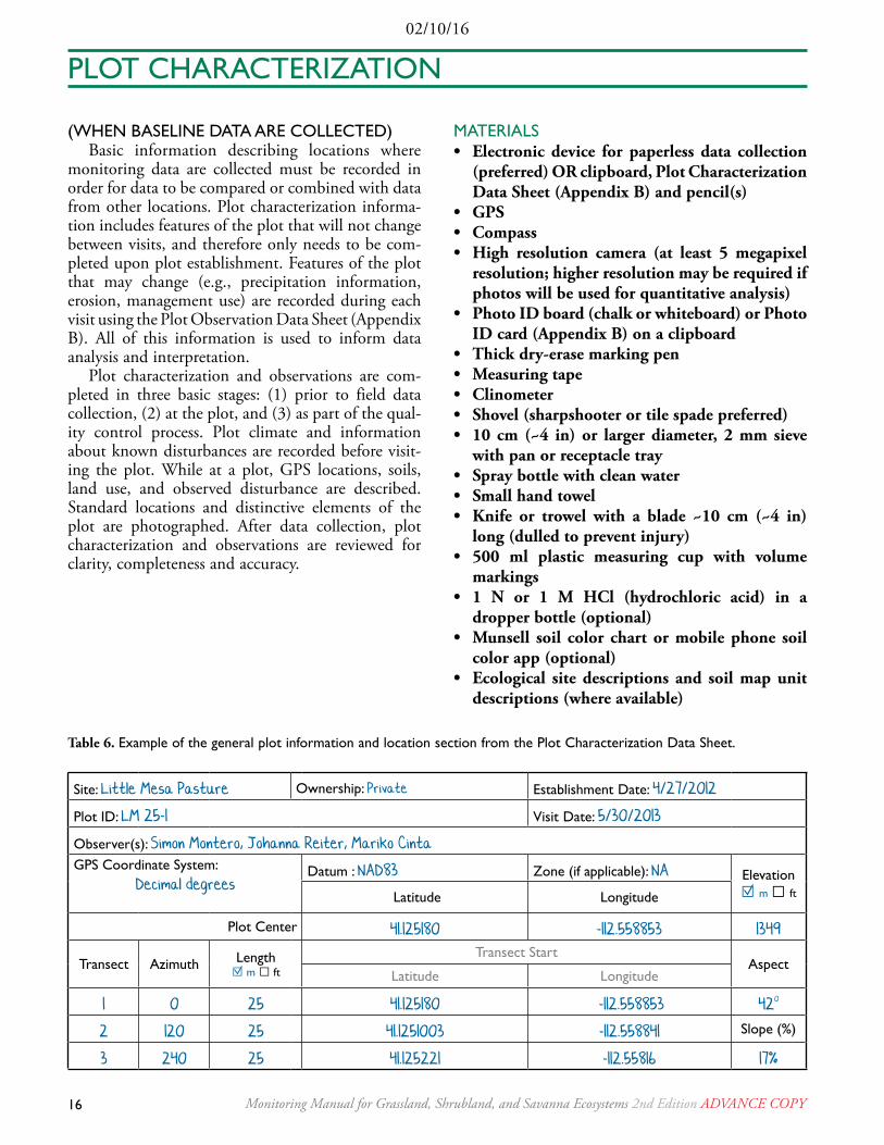
Table 6. Example of the general plot information and location section from the Plot Characterization Data Sheet.
Site: Little Mesa Pasture Ownership: Private Establishment Date: 4/27/2012
Plot ID: LM 25-1 Visit Date: 5/30/2013
Observer(s): Simon Montero, Johanna Reiter, Mariko CintaGPS Coordinate System:
Decimal degreesDatum : NAD83 Zone (if applicable): NA Elevation
☐ m ☐ ft Latitude Longitude
Plot Center 41.125180 -112.558853 1349
Transect Azimuth Length☐ m ☐ ft
Transect StartAspect
Latitude Longitude
1 0 25 41.125180 -112.558853 420
2 120 25 41.1251003 -112.558841 Slope (%)
3 240 25 41.125221 -112.55816 17%
PLOT CHARACTERIZATION
02/10/16
17Monitoring Manual for Grassland, Shrubland, and Savanna Ecosystems 2nd Edition AdvAncE copy
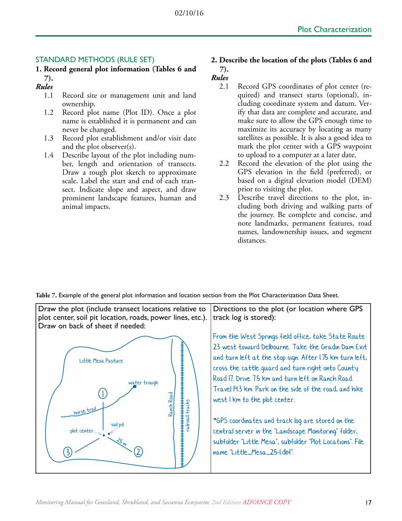
STANDARD METHODS (RULE SET)1. Record general plot information (Tables 6 and
7).Rules
1.1 Record site or management unit and land ownership.
1.2 Record plot name (Plot ID). Once a plot name is established it is permanent and can never be changed.
1.3 Record plot establishment and/or visit date and the plot observer(s).
1.4 Describe layout of the plot including num-ber, length and orientation of transects. Draw a rough plot sketch to approximate scale. Label the start and end of each tran-sect. Indicate slope and aspect, and draw prominent landscape features, human and animal impacts.
2. Describe the location of the plots (Tables 6 and 7).
Rules2.1 Record GPS coordinates of plot center (re-
quired) and transect starts (optional), in-cluding coordinate system and datum. Ver-ify that data are complete and accurate, and make sure to allow the GPS enough time to maximize its accuracy by locating as many satellites as possible. It is also a good idea to mark the plot center with a GPS waypoint to upload to a computer at a later date.
2.2 Record the elevation of the plot using the GPS elevation in the field (preferred), or based on a digital elevation model (DEM) prior to visiting the plot.
2.3 Describe travel directions to the plot, in-cluding both driving and walking parts of the journey. Be complete and concise, and note landmarks, permanent features, road names, landownership issues, and segment distances.
Table 7. Example of the general plot information and location section from the Plot Characterization Data Sheet.
Draw the plot (include transect locations relative to plot center, soil pit location, roads, power lines, etc.). Draw on back of sheet if needed:
Directions to the plot (or location where GPS track log is stored):
From the West Springs field office, take State Route 23 west toward Delbourne. Take the Gradin Dam Exit and turn left at the stop sign. After 1.75 km turn left, cross the cattle guard and turn right onto County Road 17. Drive 7.5 km and turn left on Ranch Road. Travel 14.3 km. Park on the side of the road, and hike west 1 km to the plot center.
*GPS coordinates and track log are stored on the central server in the "Landscape Monitoring" folder, subfolder "Little Mesa", subfolder "Plot Locations". File name "Little_Mesa_25-1.dbf".
plot centersoil pit
Ranc
h Ro
ad
railr
oad
trac
ks
Little Mesa Pasture
water trough
horse trail
1
23
25 m
Plot Characterization

18 Monitoring Manual for Grassland, Shrubland, and Savanna Ecosystems 2nd Edition AdvAncE copy
02/10/16
(a) Down slope shape (vertical)
(b) Across slope shape (horizontal)
linear
convex
concave
linear
convex
concave
3. Describe the topography of the plot (Tables 6 and 8).
Rules For all 3 of these rules, consider the entire area encompassed by the transects, plus an area several meters (~25 m) outside that area. This whole area is considered one unit (the plot). Do not be overly concerned with microtopographical variation within the plot. Those can be recorded in the plot sketch and notes.
3.1 Record the vertical (down slope) and hori-zontal (across slope) shape (linear, concave, or convex) (Figure 8, Table 8). Always record vertical shape first in the coding system, then horizontal shape.
3.2 Record the slope (in percent) in the direc-tion that overland water would flow through the plot center (Table 6). Slope can be deter-mined using a clinometer.
3.3 Record the aspect of the slope (facing downslope) in degrees (e.g., 1800) based on magnetic north (Table 6). Correct for decli-nation in the office if necessary.
Table 8. Example of the topography section from the Plot Characterization Data Sheet.
Figure 8. Slope shape walking down (vertically) the longest slope (a) and across (horizontally) the longest slope (b).
Plot Characterization
Vertical (Down) Slope Shape ☑ Convex ☐ Concave ☐ Linear \Horizontal (Across) Slope Shape
☐ Convex ☑ Concave ☐ Linear
) )
\))
02/10/16
19Monitoring Manual for Grassland, Shrubland, and Savanna Ecosystems 2nd Edition AdvAncE copy
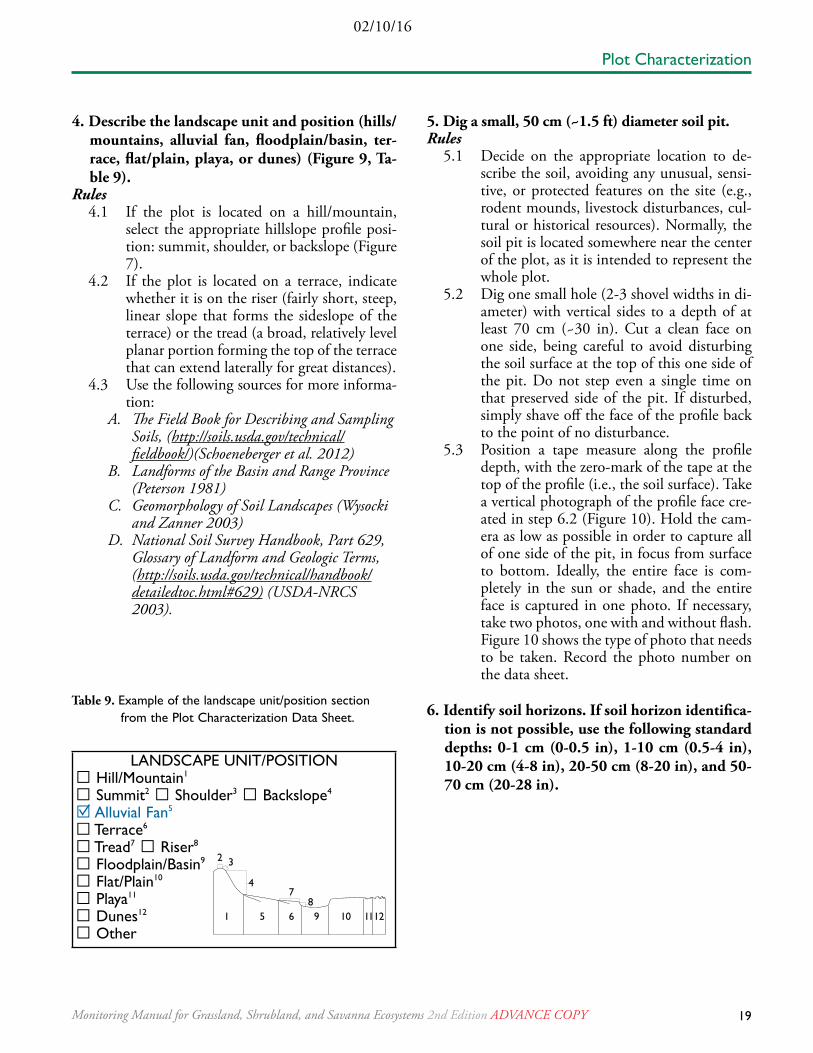
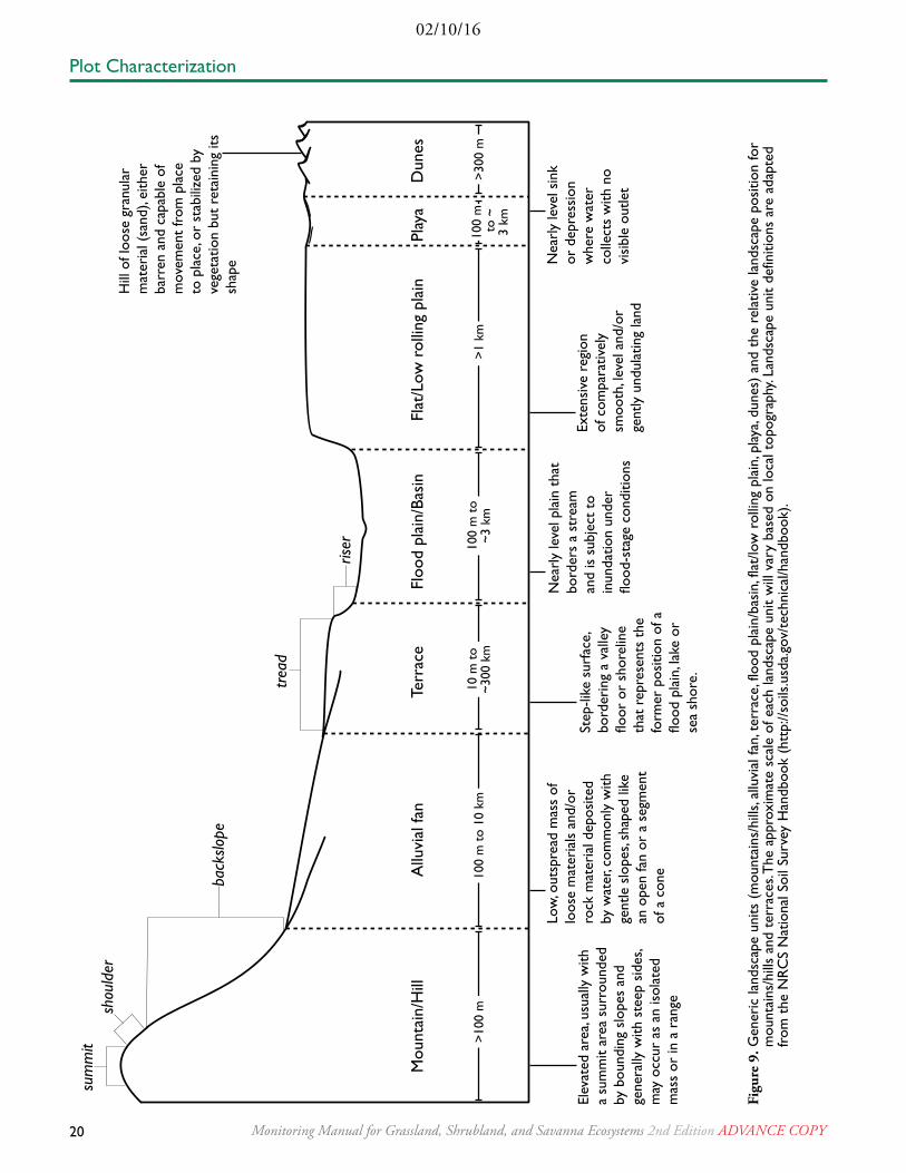
4. Describe the landscape unit and position (hills/mountains, alluvial fan, floodplain/basin, ter-race, flat/plain, playa, or dunes) (Figure 9, Ta-ble 9).
Rules4.1 If the plot is located on a hill/mountain,
select the appropriate hillslope profile posi-tion: summit, shoulder, or backslope (Figure 7).
4.2 If the plot is located on a terrace, indicate whether it is on the riser (fairly short, steep, linear slope that forms the sideslope of the terrace) or the tread (a broad, relatively level planar portion forming the top of the terrace that can extend laterally for great distances).
4.3 Use the following sources for more informa-tion:
A. The Field Book for Describing and Sampling Soils, (http://soils.usda.gov/technical/fieldbook/)(Schoeneberger et al. 2012)
B. Landforms of the Basin and Range Province (Peterson 1981)
C. Geomorphology of Soil Landscapes (Wysocki and Zanner 2003)
D. National Soil Survey Handbook, Part 629, Glossary of Landform and Geologic Terms, (http://soils.usda.gov/technical/handbook/detailedtoc.html#629) (USDA-NRCS 2003).
5. Dig a small, 50 cm (~1.5 ft) diameter soil pit.Rules
5.1 Decide on the appropriate location to de-scribe the soil, avoiding any unusual, sensi-tive, or protected features on the site (e.g., rodent mounds, livestock disturbances, cul-tural or historical resources). Normally, the soil pit is located somewhere near the center of the plot, as it is intended to represent the whole plot.
5.2 Dig one small hole (2-3 shovel widths in di-ameter) with vertical sides to a depth of at least 70 cm (~30 in). Cut a clean face on one side, being careful to avoid disturbing the soil surface at the top of this one side of the pit. Do not step even a single time on that preserved side of the pit. If disturbed, simply shave off the face of the profile back to the point of no disturbance.
5.3 Position a tape measure along the profile depth, with the zero-mark of the tape at the top of the profile (i.e., the soil surface). Take a vertical photograph of the profile face cre-ated in step 6.2 (Figure 10). Hold the cam-era as low as possible in order to capture all of one side of the pit, in focus from surface to bottom. Ideally, the entire face is com-pletely in the sun or shade, and the entire face is captured in one photo. If necessary, take two photos, one with and without flash. Figure 10 shows the type of photo that needs to be taken. Record the photo number on the data sheet.
6. Identify soil horizons. If soil horizon identifica-tion is not possible, use the following standard depths: 0-1 cm (0-0.5 in), 1-10 cm (0.5-4 in), 10-20 cm (4-8 in), 20-50 cm (8-20 in), and 50-70 cm (20-28 in).
Table 9. Example of the landscape unit/position section from the Plot Characterization Data Sheet.
Plot Characterization
LANDSCAPE UNIT/POSITION☐ Hill/Mountain1
☐ Summit2 ☐ Shoulder3 ☐ Backslope4
☐ Alluvial Fan5 ☐ Terrace6 ☐ Tread7 ☐ Riser8 ☐ Floodplain/Basin9 ☐ Flat/Plain10 ☐ Playa11
☐ Dunes12
☐ Other1 5 6 9 10 1112
2 3
47
8
20 Monitoring Manual for Grassland, Shrubland, and Savanna Ecosystems 2nd Edition AdvAncE copy
02/10/16
tread
riser
sum
mit
shou
lder
back
slope
Mou
ntai
n/H
illA
lluvi
al fa
nTe
rrac
eFl
ood
plai
n/Ba
sin
Flat
/Low
rol
ling
plai
nPl
aya
Dun
es
>100
m10
0 m
to
10 k
m10
m t
o ~3
00 k
m10
0 m
to
~3 k
m
>1
km>3
00 m
Nea
rly
leve
l sin
k or
dep
ress
ion
whe
re w
ater
co
llect
s w
ith n
o vi
sibl
e ou
tlet
Hill
of l
oose
gra
nula
r m
ater
ial (
sand
), ei
ther
ba
rren
and
cap
able
of
mov
emen
t fr
om p
lace
to
pla
ce, o
r st
abili
zed
by
vege
tatio
n bu
t re
tain
ing
its
shap
e
Low
, out
spre
ad m
ass
of
loos
e m
ater
ials
and
/or
rock
mat
eria
l dep
osite
d by
wat
er, c
omm
only
with
ge
ntle
slo
pes,
shap
ed li
ke
an o
pen
fan
or a
seg
men
t of
a c
one
Step
-like
sur
face
, bo
rder
ing
a va
lley
floor
or
shor
elin
e th
at r
epre
sent
s th
e fo
rmer
pos
ition
of a
flo
od p
lain
, lak
e or
se
a sh
ore.
Nea
rly
leve
l pla
in t
hat
bord
ers
a st
ream
an
d is
sub
ject
to
inun
datio
n un
der
flood
-sta
ge c
ondi
tions
Exte
nsiv
e re
gion
of
com
para
tivel
y sm
ooth
, lev
el a
nd/o
r ge
ntly
und
ulat
ing
land
Elev
ated
are
a, us
ually
with
a
sum
mit
area
sur
roun
ded
by b
ound
ing
slop
es a
nd
gene
rally
with
ste
ep s
ides
, m
ay o
ccur
as
an is
olat
ed
mas
s or
in a
ran
ge
Figu
re 9
. Gen
eric
land
scap
e un
its (
mou
ntai
ns/h
ills,
allu
vial
fan,
ter
race
, flo
od p
lain
/bas
in, f
lat/
low
rol
ling
plai
n, p
laya
, dun
es)
and
the
rela
tive
land
scap
e po
sitio
n fo
r m
ount
ains
/hill
s an
d te
rrac
es. T
he a
ppro
xim
ate
scal
e of
eac
h la
ndsc
ape
unit
will
var
y ba
sed
on lo
cal t
opog
raph
y. La
ndsc
ape
unit
defin
ition
s ar
e ad
apte
d fr
om t
he N
RC
S N
atio
nal S
oil S
urve
y H
andb
ook
(htt
p://s
oils
.usd
a.go
v/te
chni
cal/h
andb
ook)
.
Plot Characterization
100
m t
o ~
3
km
02/10/16
21Monitoring Manual for Grassland, Shrubland, and Savanna Ecosystems 2nd Edition AdvAncE copy
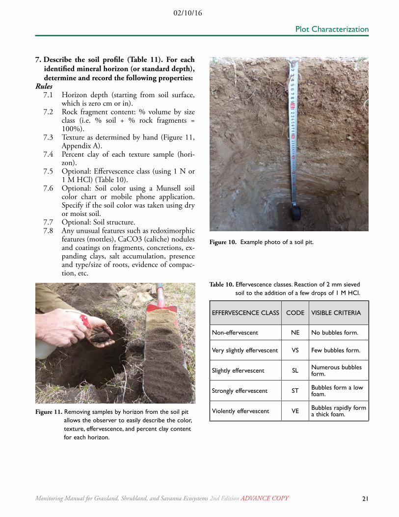
Figure 10. Example photo of a soil pit.
Figure 11. Removing samples by horizon from the soil pit allows the observer to easily describe the color, texture, effervescence, and percent clay content for each horizon.
Table 10. Effervescence classes. Reaction of 2 mm sieved soil to the addition of a few drops of 1 M HCl.
EFFERVESCENCE CLASS CODE VISIBLE CRITERIA
Non-effervescent NE No bubbles form.
Very slightly effervescent VS Few bubbles form.
Slightly effervescent SL Numerous bubbles form.
Strongly effervescent ST Bubbles form a low foam.
Violently effervescent VE Bubbles rapidly form a thick foam.
7. Describe the soil profile (Table 11). For each identified mineral horizon (or standard depth), determine and record the following properties:
Rules7.1 Horizon depth (starting from soil surface,
which is zero cm or in).7.2 Rock fragment content: % volume by size
class (i.e. % soil + % rock fragments = 100%).
7.3 Texture as determined by hand (Figure 11, Appendix A).
7.4 Percent clay of each texture sample (hori-zon).
7.5 Optional: Effervescence class (using 1 N or 1 M HCl) (Table 10).
7.6 Optional: Soil color using a Munsell soil color chart or mobile phone application. Specify if the soil color was taken using dry or moist soil.
7.7 Optional: Soil structure.7.8 Any unusual features such as redoximorphic
features (mottles), CaCO3 (caliche) nodules and coatings on fragments, concretions, ex-panding clays, salt accumulation, presence and type/size of roots, evidence of compac-tion, etc.
Plot Characterization
22 Monitoring Manual for Grassland, Shrubland, and Savanna Ecosystems 2nd Edition AdvAncE copy
02/10/16
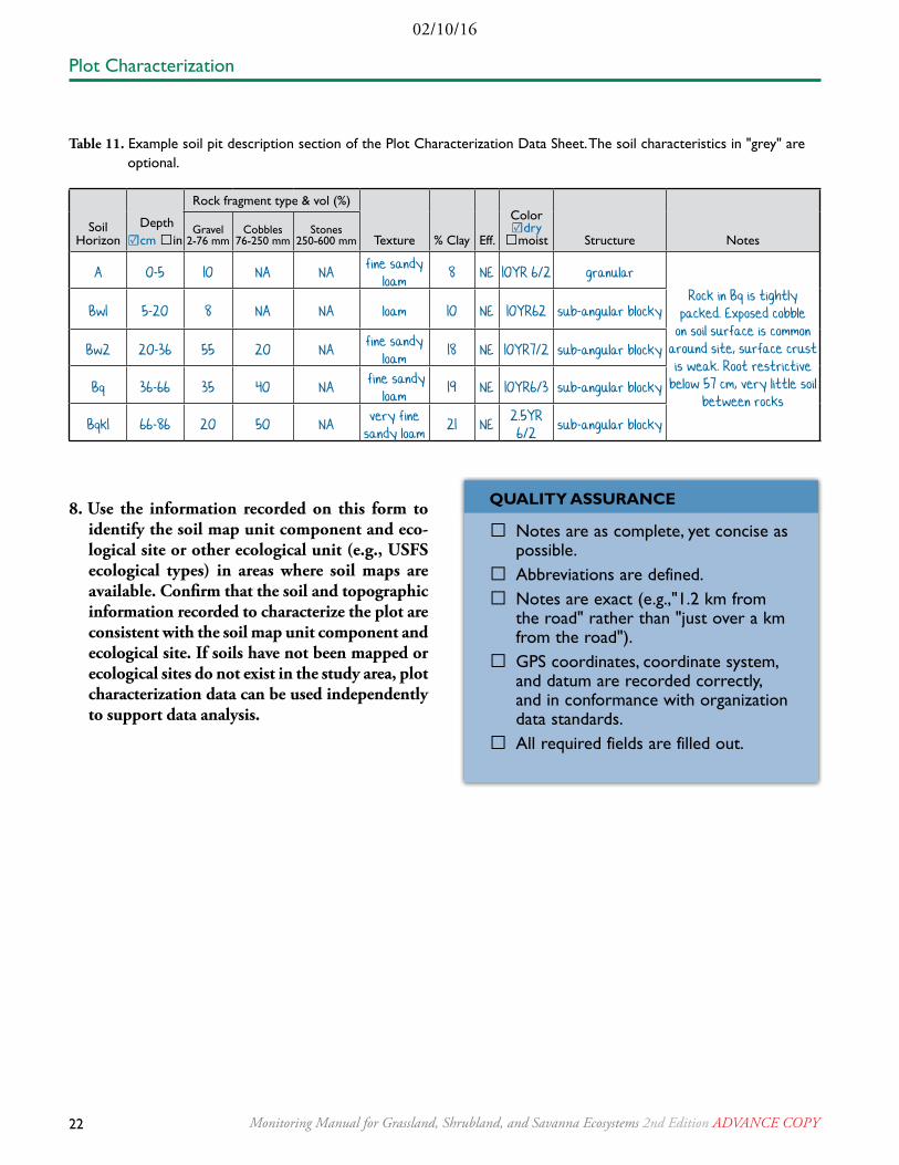
Soil Horizon
Depth☑cm ☐in
Rock fragment type & vol (%)
Texture % Clay Eff.
Color☑dry
☐moist Structure NotesGravel
2-76 mmCobbles
76-250 mmStones
250-600 mm
A 0-5 10 NA NAfine sandy
loam8 NE 10YR 6/2 granular
Rock in Bq is tightly packed. Exposed cobble
on soil surface is common around site, surface crust is weak. Root restrictive
below 57 cm, very little soil between rocks
Bw1 5-20 8 NA NA loam 10 NE 10YR62 sub-angular blocky
Bw2 20-36 55 20 NAfine sandy
loam18 NE 10YR7/2 sub-angular blocky
Bq 36-66 35 40 NA fine sandy
loam19 NE 10YR6/3 sub-angular blocky
Bqk1 66-86 20 50 NAvery fine
sandy loam21 NE
2.5YR 6/2
sub-angular blocky
Table 11. Example soil pit description section of the Plot Characterization Data Sheet. The soil characteristics in "grey" are optional.
8. Use the information recorded on this form to identify the soil map unit component and eco-logical site or other ecological unit (e.g., USFS ecological types) in areas where soil maps are available. Confirm that the soil and topographic information recorded to characterize the plot are consistent with the soil map unit component and ecological site. If soils have not been mapped or ecological sites do not exist in the study area, plot characterization data can be used independently to support data analysis.
Plot Characterization
QUALitY AssURAnCE
☐ Notes are as complete, yet concise as possible.
☐ Abbreviations are defined. ☐ Notes are exact (e.g.,"1.2 km from the road" rather than "just over a km from the road").
☐ GPS coordinates, coordinate system, and datum are recorded correctly, and in conformance with organization data standards.
☐ All required fields are filled out.
02/10/16
23Monitoring Manual for Grassland, Shrubland, and Savanna Ecosystems 2nd Edition AdvAncE copy
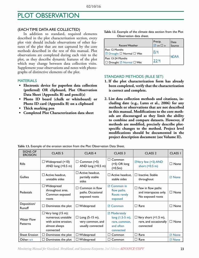
(EACH TIME DATA ARE COLLECTED) In addition to standard, required elements
described in the plot characterization section, every plot visit should include observations of other fea-tures of the plot that are not captured by the core methods described in the rest of this manual. Plot observations are completed during each visit to the plot, as they describe dynamic features of the plot which may change between data collection visits. Supplement your observations and notes with photo-graphs of distinctive elements of the plot.
MATERIALS• Electronic device for paperless data collection
(preferred) OR clipboard, Plot Observation Data Sheet (Appendix B) and pencil(s)
• Photo ID board (chalk or whiteboard) or Photo ID card (Appendix B) on a clipboard
• Thick marking pen• Completed Plot Characterization data sheet
STANDARD METHODS (RULE SET)1. If the plot characterization form has already
been completed, verify that the characterization is correct and complete.
2. List data collection methods and citations, in-cluding date (e.g., Lutes et al., 2006) for any methods or observations that are not described in this manual. Modifications to the core meth-ods are discouraged as they limit the ability to combine and compare datasets. However, if methods are modified, precisely describe plot-specific changes to the method. Project level modifications should be documented in the project description document (see Volume II).
PLOT OBSERVATION
SIGNS OF EROSION CLASS 5 CLASS 4 CLASS 3 CLASS 2 CLASS 1
Rills☐ Widespread (>10)
AND long (>0.5 m)☐ Common (>5)
AND long (>0.5 m)
☐ Common (>5) OR long (>0.5m)
☑Very few (<5) AND short (<0.5 m)
☐ None
Gullies☐ Active headcut,
unstable sides
☐ Active headcut, partially stable sides
☐ Active headcut, stable sides
☐ Inactive. Stable throughout
☑ None
Pedestals
☐ Widespread throughout area. Common exposed roots
☐ Common in flow paths. Occasional exposed roots
☑ Common in flow paths. Roots rarely exposed
☐ Few in flow paths and interspaces only. No exposed roots
☐ None
Deposition/Runoff
☐ Dominates the plot ☐ Widespread ☑ Common ☐ Rare ☐ None
Water Flow Patterns
☐ Very long (15 m); numerous; unstable with active erosion; almost always connected
☐ Long (5-15 m), very common, and usually connected
☑ Moderately long (1.5-5 m), rare, common, and often connected
☐ Very short (<1.5 m), rare, and occasionally connected
☐ None
Sheet Erosion ☐ Dominates the plot ☐ Widespread ☐ Common ☐ Rare ☑ NoneOther: N/A ☐ Dominates the plot ☐ Widespread ☐ Common ☐ Rare ☑ None
Recent WeatherPrecip.☑ cm ☐ in
Data Source
Past 12 Months☑ Drought ☐ Normal ☐ Wet 13.4
NOAAPast 13-24 Months☐ Drought ☑ Normal ☐ Wet 22.4
Table 12. Example of the climate data section from the Plot Observation data sheet.
Table 13. Example of the erosion section from the Plot Observation Data Sheet.
24 Monitoring Manual for Grassland, Shrubland, and Savanna Ecosystems 2nd Edition AdvAncE copy
02/10/16
Table 14. Example of the land use section from the Plot Observation Data Sheet.Describe management history (e.g., grazing plan, prescribed fire, shrub control, seeding, plowing, water units): Office records show that the site burned in 2002. A shrub/perennial bunch grass mix was seeded aerially as part of the rehabilitation.
Describe wildlife use (note types, species identified, and condition): Saw 6 wild horses while hiking to the plot. Horse trail intersects Line 1. Observed herd of ~20 pronghorn ~ 1 km north of the plot.Describe livestock use (note species, evidence, and intensity):Cattle in area but not directly on plot. A livestock watering trough is located 500 m NE of the plot.Describe off-site influences (e.g., transmission lines, mines, roads): Ranch Road, a graded dirt road, is 1.2 km east of the plot, railroad tracks run parallel to Ranch RoadAdditional visible disturbances and remarks (e.g., invasive species, evidence of fire, pests and pathogens): Invasive species (BRTE, HAGL) are dominant on the plot. The area burned as part of the James Fire in 2002.
3. Describe the weather (events affecting plots that day) of the plot (Table 12). Do this prior to visiting the plot, using data from sources such as the Western Regional Climate Center (http://www.wrcc.dri.edu), PRISM (http://prism.orgeonstate.edu), or NOAA (http://www.ncdc.noaa.gov), and then describe any on-site evidence (e.g., evidence of a large, recent runoff event) that would appear to confirm or contra-dict online information.
Rules3.1 Record annual precipitation for the past 12
months and the past 13 to 24 months.3.2 Note whether these are normal, drought, or
wet conditions.3.3 Record the precipitation data source.
4. Note signs of erosion (if any) (Table 13). Rules
4.1 Note signs of water movement over the plot (e.g., gullies, rills, litter dams, vegetation or rock pedestals, water flow patterns, sheet erosion).
4.2 Note signs of wind erosion (e.g., wind-scoured blow outs, soil deposition around plants).
5. Describe previous land use, treatments, distur-bances or other known management actions on the plot. For repeat (monitoring) visits, focus on change in management or other disturbanc-es since the last visit (Table 14).
6. Describe current land use of the plot area (Table 14). Be sure to photograph unusual features.
Rules6.1 Note wildlife or evidence of wildlife (e.g.,
rodent burrows, droppings).6.2 Note evidence and intensity of livestock use.
7. Describe off-site influences such as roads, wa-ter sources, mining, and housing developments (Table 14).
Plot Observation
QUALitY AssURAnCE
☐ Notes are as complete, yet concise as possible.
☐ Abbreviations are defined. ☐ Notes are exact (e.g.,"10 year old native grass seeding treatment is 200 m north of the plot " rather than "seeding treatment next to plot”).
☐ Notes are descriptive (e.g.,"cattle trailing on SW corner of plot" rather than "trailing on plot").

02/10/16
25Monitoring Manual for Grassland, Shrubland, and Savanna Ecosystems 2nd Edition AdvAncE copy
Use Photo points to qualitatively monitor how vegetation changes over time. Repeat photographs of a landscape are useful for detecting changes in vegeta-tion structure, major soil redistribution patterns, and for visually documenting measured changes. Photos are also vital for relocating a plot or transect on subse-quent visits. Another important role of photos is to aid in verification and interpretation of quantitative data back in the office. Take at least one photo of each tran-sect before collecting other measurements. If you take digital photos, be sure to back-up and securely archive the image files. You may also want to print and store photos in plastic photo storage sheets. Slide the Photo ID card (Appendix B) behind the photo in the plastic storage sheet. For more information on photo point monitoring, see the USFS Photo Point Monitoring Handbook (www.fs.fed.us/pnw/pubs/gtr526/).
MATERIALS• Tape measure (5 m (15 ft) minimum)• Compass• High resolution camera (at least 5 megapixel
capacity)• Photo ID board (chalk or whiteboard) or Photo
ID card (Appendix B) on a clipboard• Thick marking pen or dry-erase marker in a
dark color• One 1.5 m (5 ft) long, 3/4-in diameter PVC pipe
STANDARD METHODS (RULE SET)1. Set up first photo (Figure 12).Rules
1.1 Prepare a legible Photo ID board and rest it against the transect stake at the beginning of the first transect. Make sure all written letter-ing is thick and clear. Ensure no vegetation obstructs writing on the ID board. If neces-sary, a colleague may hold the ID board so that it is visible in front of vegetation, stay-ing as low and unobtrusive as possible.
1.2 Stand back 5 m (15 feet) from the start of the transect. This is the camera location, and is in line with the bearing of the transect.
1.3 If project protocols allow, mark the camera point using a rebar stake, metal post, PVC pipe, rock cairn, or other permanent, un-obstructive marker. A permanent camera marker will enable higher precision in posi-tioning and repeating the photo in succeed-ing years.
2. Take first photo (Figures 12 and 13).Rules
2.1 Set camera body on top of the 1.5 m (5 ft) PVC pipe and point the camera lens toward the first transect such that the photo will be taken in landscape orientation. The bottom of the pipe should rest on the ground.
2.2 Place lower edge of photo ID board at the photo’s bottom center, but leave a tiny amount of space below the board. This demonstrates to future viewers that all data on the board has been photographed, and has not been cut off.
2.3 Signal data collection crew to exit the field of view.
2.4 Adjust the camera's field of view to mini-mum zoom and infinite focus settings. Do not use a flash, if possible. A flash will dis-tort the foreground appearance and is in-effective past a few meters out. It is best to take photos with ample daylight, but if forced to photograph in low-light condi-tions, increase the exposure settings on the camera rather than use flash.
2.5 If photos were taken on the plot in the past, make sure current photos are taken at the same distance from the transect, com-pass bearing, and with the same horizon as photos from the past.
2.6 Take photo and immediately check that it saved to the camera's memory card.
2.7 If tall vegetation or large rocks obstruct all of the transect from the original camera setup point, take a second photo at a lo-cation further down the transect, pointing in the same direction. Note the new camera position on the ID board
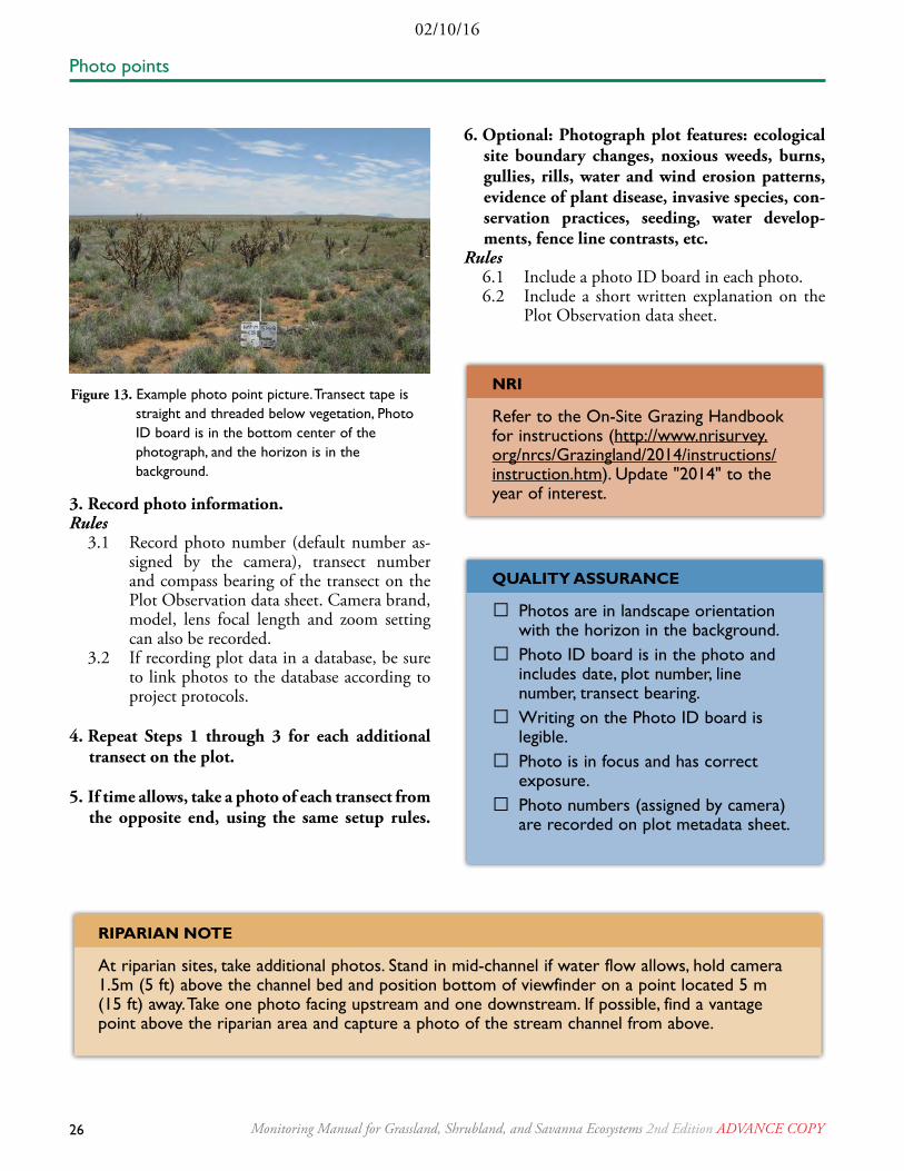
Figure 12. Photo point layout.
PHOTO POINTS
26 Monitoring Manual for Grassland, Shrubland, and Savanna Ecosystems 2nd Edition AdvAncE copy
02/10/16
6. Optional: Photograph plot features: ecological site boundary changes, noxious weeds, burns, gullies, rills, water and wind erosion patterns, evidence of plant disease, invasive species, con-servation practices, seeding, water develop-ments, fence line contrasts, etc.
Rules6.1 Include a photo ID board in each photo.6.2 Include a short written explanation on the
Plot Observation data sheet.
Figure 13. Example photo point picture. Transect tape is straight and threaded below vegetation, Photo ID board is in the bottom center of the photograph, and the horizon is in the background.
3. Record photo information.Rules
3.1 Record photo number (default number as-signed by the camera), transect number and compass bearing of the transect on the Plot Observation data sheet. Camera brand, model, lens focal length and zoom setting can also be recorded.
3.2 If recording plot data in a database, be sure to link photos to the database according to project protocols.
4. Repeat Steps 1 through 3 for each additional transect on the plot.
5. If time allows, take a photo of each transect from the opposite end, using the same setup rules.
Photo points
RipARiAn nOtE
At riparian sites, take additional photos. Stand in mid-channel if water flow allows, hold camera 1.5m (5 ft) above the channel bed and position bottom of viewfinder on a point located 5 m (15 ft) away. Take one photo facing upstream and one downstream. If possible, find a vantage point above the riparian area and capture a photo of the stream channel from above.
nRi
Refer to the On-Site Grazing Handbook for instructions (http://www.nrisurvey.org/nrcs/Grazingland/2014/instructions/instruction.htm). Update "2014" to the year of interest.
QUALitY AssURAnCE
☐ Photos are in landscape orientation with the horizon in the background.
☐ Photo ID board is in the photo and includes date, plot number, line number, transect bearing.
☐ Writing on the Photo ID board is legible.
☐ Photo is in focus and has correct exposure.
☐ Photo numbers (assigned by camera) are recorded on plot metadata sheet.

02/10/16
27Monitoring Manual for Grassland, Shrubland, and Savanna Ecosystems 2nd Edition AdvAncE copy
Line-point intercept is a rapid, accurate method for quantifying soil cover, including vegetation, lit-ter, rocks and biological crusts. These measurements are related to wind and water erosion, water infiltra-tion, and the ability of the site to resist and recover from disturbance. Line-point intercept can be mea-sured together with Vegetation height, which describes vertical vegetation structure. For a detailed discussion of this and other methods for measuring plant cover and/or composition, see Elzinga et al. 20012.
MATERIALS• Measuring tape (length of transect)—if using
a tape measure in feet, use one marked in tenths of feet
• Two steel stakes for anchoring tape• One pointer—a straight piece of wire or
rod, such as a long pin flag, at least 75 cm (2.5 ft) long and 1 mm (0.04 in) or less in diameter
• Electronic device for paperless data collection (preferred) OR clipboard, Line-point Intercept Data Sheet (Appendix B) and pencil(s)
STANDARD METHODS (RULE SET) 1. Pull out the tape and anchor each end with
a steel stake. See the instructions on stringing a tape on page 6.
2. As you move from one end of the tape to the other, always stand on the same side (the south side for NRI) of the transect for all methods and measurements. Move to the first point (0 mark) on the tape.
2 Elzinga, C.L., D.W. Salzer, J.W. Willoughby and J.P. Gibbs. 2001. Monitoring Plant and Animal Populations, Blackwell Publishing. 368 pp.
3. Drop a pin flag to the ground from a standard height next to the tape (Figure 14).
Rules3.1 Keep the pin vertical.3.2 Make a "controlled drop" of the pin from
the same height each time. Position the pin so its lower end is several centimeters above the vegetation, release it and allow it to slip through the hand until it hits the ground. A low drop height minimizes “bounces” off of vegetation but increases the possibility for bias.
3.3 Do not guide the pin all the way to the ground. It is more important for the pin to fall freely to the ground than to fall precisely on the transect tape mark.
3.4 A laser with a bubble level can be used in-stead of the pin. This tool is useful in eco-systems where plant layers may be above eye level. See Appendix A (Monitoring tools) in Volume II for suppliers.
4. Once the pin flag is flush with the ground, re-cord every plant species it intercepts (Tables 15 and 16).
Rules4.1 Record the species of the uppermost or first
stem, leaf or plant base intercepted in the “Top layer” column, using the PLANTS Database species code (http://plants.usda.gov), a code based on the first two letters of the genus and species, or the common name.
Figure 14. Point falling on bare soil (N/S).
LINE-POINT INTERCEPT
HELpfUL tip
If Gap intercept is also measured, it is most efficient to measure Gap intercept starting from "0" to the end of the transect, and for Line-point intercept to be read from the end of the transect back to "0".
28 Monitoring Manual for Grassland, Shrubland, and Savanna Ecosystems 2nd Edition AdvAncE copy
02/10/16
4.2 If no leaf, stem or plant base is intercepted or touches the pin, record “N” for none in the “Top layer” column.
4.3 Record all additional species intercepted by the pin, in the order that they are intercept-ed, from top to bottom.
4.4 Record herbaceous litter as "HL", if pres-ent. Herbaceous litter is defined as detached stems, roots, leaves, haybales, and dung. Re-cord “WL” for detached woody or succulent litter that is greater than 5 mm (or ~1/4 in) in diameter. Record "NL" for non-vegetative litter (e.g., plastic, metal, decomposing ani-mal matter).
4.5 Record each plant species only once, the first time it is intercepted, even if it is intercepted several times.
4.6 If a plant species is not known, use the following codes, adding sequential numbers as necessary:AF# = Annual forb (also includes biennials)PF# = Perennial forbAG# = Annual graminoidPG# = Perennial graminoidSH# = Shrub TR# = TreeIf necessary, collect a sample of unknown plants off the transect for later identification (see page 14) for voucher specimen collec-tion protocols).
4.7 If the genus is known, but not the species, either use the PLANTS Database genus code (http://plants.usda.gov) or record an unknown plant code as described above and note the genus at the bottom of the data sheet.
4.8 Foliage can be live or dead (see inset box), but only record each species once in at each pin drop. If both live and dead canopy for the same species is hit on the same point, record the live canopy.
4.9 Record vagrant lichen as "VL" or by its spe-cies in the lower layer columns.
4.10 In environments where deposited soil over a plant base occurs (Figures 15-16), push the pin below the soil surface. Gently move the pin from side to side to feel for buried plant bases. If resistance from the plant base is
encountered, record deposited soil as "DS" in the lower canopy and record the spe-cies basal hit in the "Soil Surface" column.
5. Record a species code (if the pin flag intercepts a plant base, Figure 16) or another soil surface code in the “Soil surface” column (Table 15).
Rules5.1 For unidentified plant bases, use the codes
listed under Rule 4.6.5.2 An intercept with a plant base is defined as
when the end of the pin rests either on, or immediately adjacent to and touching, liv-ing or dead plant material that is rooted in the soil. Carefully scrutinize if the pin is touching small, single-stemmed plants.
6. Optional: Add more specific soil surface categories. 6.1 Record “CY” or dark cyanobacterial crust.6.2 If mosses and lichens are identified to spe-
cies, record the species code in the "Soil sur-face" column.
Line-point intercept
nRi
Measure in English units
RECORding dEAd vs. LivE
Distinguishing dead vs. live plant parts is important for many objectives. A pin intercept is a standing dead hit if the pin touches a dead plant part. • Vegetation which grew in the current
growing season is alive while rooted vegetation from the previous growing season is dead.
• Perennial and woody plant parts which support live vegetation are alive.
• Points where only dead plants or plant parts are intercepted can be recorded on paper by circling the species on paper data sheets, or electronically (by using the optional checkbox in the DIMA Line-point intercept form (http://jornada.nmsu.edu/monit-assess/).
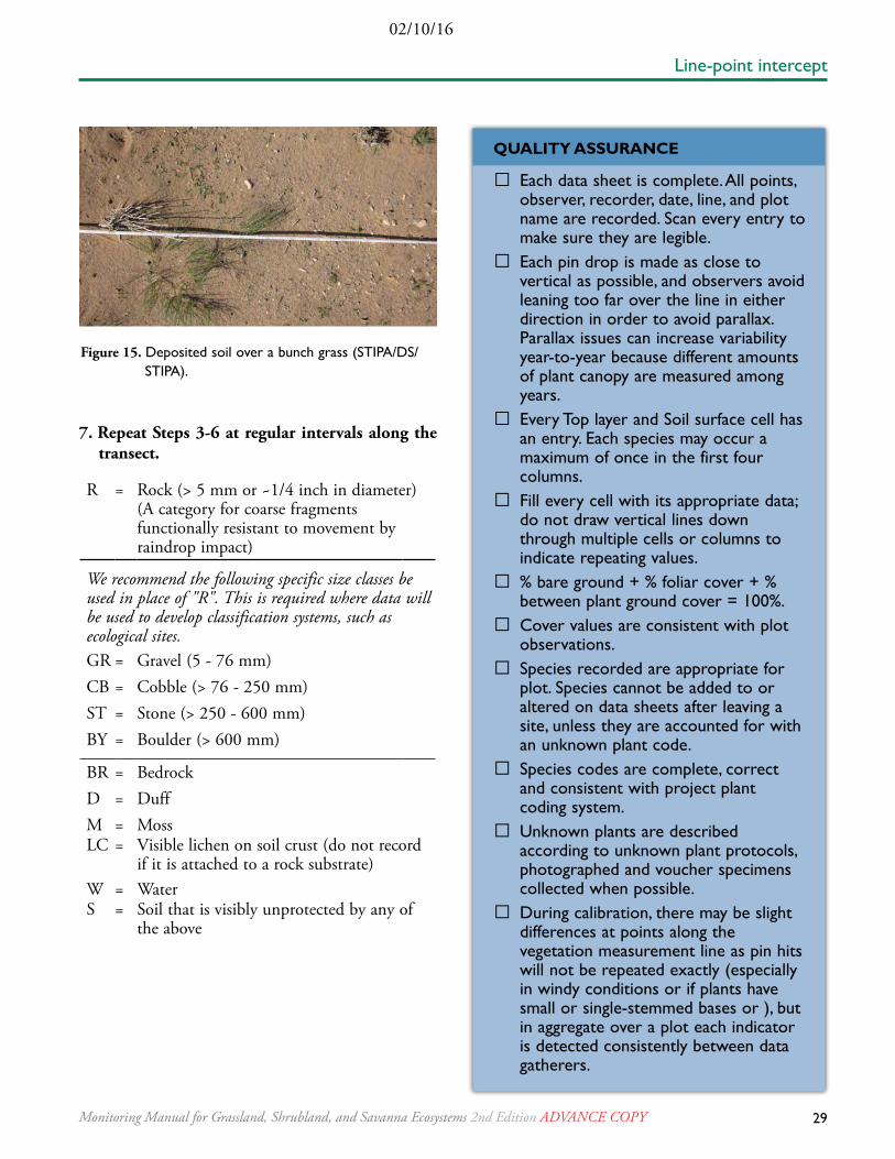
02/10/16
29Monitoring Manual for Grassland, Shrubland, and Savanna Ecosystems 2nd Edition AdvAncE copy
Figure 15. Deposited soil over a bunch grass (STIPA/DS/STIPA).
R = Rock (> 5 mm or ~1/4 inch in diameter) (A category for coarse fragments functionally resistant to movement by raindrop impact)
We recommend the following specific size classes be used in place of "R". This is required where data will be used to develop classification systems, such as ecological sites. GR = Gravel (5 - 76 mm)CB = Cobble (> 76 - 250 mm)ST = Stone (> 250 - 600 mm)BY = Boulder (> 600 mm)
BR = BedrockD = DuffM = MossLC = Visible lichen on soil crust (do not record
if it is attached to a rock substrate)W = WaterS = Soil that is visibly unprotected by any of
the above
Line-point intercept
QUALitY AssURAnCE
☐ Each data sheet is complete. All points, observer, recorder, date, line, and plot name are recorded. Scan every entry to make sure they are legible.
☐ Each pin drop is made as close to vertical as possible, and observers avoid leaning too far over the line in either direction in order to avoid parallax. Parallax issues can increase variability year-to-year because different amounts of plant canopy are measured among years.
☐ Every Top layer and Soil surface cell has an entry. Each species may occur a maximum of once in the first four columns.
☐ Fill every cell with its appropriate data; do not draw vertical lines down through multiple cells or columns to indicate repeating values.
☐ % bare ground + % foliar cover + % between plant ground cover = 100%.
☐ Cover values are consistent with plot observations.
☐ Species recorded are appropriate for plot. Species cannot be added to or altered on data sheets after leaving a site, unless they are accounted for with an unknown plant code.
☐ Species codes are complete, correct and consistent with project plant coding system.
☐ Unknown plants are described according to unknown plant protocols, photographed and voucher specimens collected when possible.
☐ During calibration, there may be slight differences at points along the vegetation measurement line as pin hits will not be repeated exactly (especially in windy conditions or if plants have small or single-stemmed bases or ), but in aggregate over a plot each indicator is detected consistently between data gatherers.
7. Repeat Steps 3-6 at regular intervals along the transect.

30 Monitoring Manual for Grassland, Shrubland, and Savanna Ecosystems 2nd Edition AdvAncE copy
02/10/16
Table 15. A list of columns that can be populated as part of Line-point intercept, along with a list of permitted options for each column. Following these protocols facilitates simple calculations on paper data sheets, and consistent calculations with electronically recorded data.
LPI COLUMN PERMITTED OPTIONS SOURCE/CODE DESCRIPTION
Top layer codes
N Indicates no foliar cover.Plant code From PLANTS Database
Foliar cover.Unknown plant code User assigned code
Lower codes
Plant code From PLANTS DatabaseFoliar cover.
Unknown plant code User assigned code
Litter
HL - herbaceous litter (including dung and haybales)
Litter cannot be entered above the first plant code or in the Top layer.
WL - woody or succulent litter > 5 mm diameterNL - other litter such as plastic, metal, and decomposing animal matter
Opt
iona
l
Otherwise record:Deposited soil DS S on Soil surface Soil deposition overlying a plant base.
Water W W on Soil surface Water or ice present at the time of measurement. May be permanent or ephemeral.
Vagrant lichen VL Litter Lichens that are loose, never attached to any substrate.
Rock fragment
GR - gravel GR or R on soil sur face
Rock fragments 5 - 76 mm, but only when overlying a buried plant base.
CB - cobble CB or R on soil surface
Rock fragments 76 - 250 mm, but only when overlying a buried plant base.
ST- stone ST or R on soil surface
Rock fragments 250 - 600 mm, but only when overlying a buried plant base.
Soil surface codes
Plant code From PLANTS DatabaseIndicates pin on hit a plant base. Plant bases have no minimum height, record a foliar hit of the same species above any plant basal hit even when no apparent pin contact is made with a leaf or stem.Unknown plant User assigned code
Soil S Indicates bare soil, mineral soil, or soil with no detectable biological crust.
Lichen LC (or species code if known*) Visible lichen crust attached to soil surface. Record if attached to soil, but not if on rock.
Moss M (or species code if known*)
Duff D Partially decomposed plant litter with no recognizable plant parts.
Water W Permanent water
Rock fragment R All rock fragments > 5 mm (do not use GR,CB, ST, or By because R represents all of these).
Opt
iona
l
Otherwise, record:
Cyanobacteria Cy SFor consistency with NRI bare ground calculations, both "N/S" and "N/Cy" pin hits constitute bare ground.
Embedded litter ELL in lower canopy and S on the Soil surface
Embedded woody litter > 5 mm in diameter
GR - gravel R Rock fragments 5 - 76 mm.CB - cobble R Rock fragments 76 - 250 mm.ST - stone R Rock fragments 250 - 600 mm.By- boulder R Rock fragments > 600 mm.BR - bedrock R
Line-point intercept

02/10/16
31Monitoring Manual for Grassland, Shrubland, and Savanna Ecosystems 2nd Edition AdvAncE copy
Pin flag
Bluegrass(live)
Clover (live)
Litter
SoilGravel
Fescue(live)
Fescue(dead)
Pin flag
Litter
Soil
Fescue(dead)
Point 2
Table 16. Sample data sheet for examples illustrated below. Points 1 and 2 show the first two points on a transect. In Point 1, the pin flag is touching dead fescue (FERU2), live bluegrass (POPR), clover (TRRE3), live fescue, litter, and a rock. Record fescue only once, even though it intercepts the pin twice. In Point 2, the flag touches fescue, then touches litter, and finally the fescue plant base.
Gravel
Figure 16. Area defined as plant base and included as basal cover.
Point 1
PT.TOP
LAyER
LOWER LAyERS SOIL SURFACECODE 1 CODE 2 CODE 3
1 FERU2 POPR TRRE3 HL R2 FERU2 HL FERU23 FERU2 HL S4 N S
etc.
Plant base
Basal cover
Deposited soil
Line-point intercept
RipARiAn nOtE
Line-point intercept collected perpendicular to the channel is often used to monitor riparian zone width. A modified point intercept method is used to monitor “greenline” vegetation along the channel’s edge (Volume II).

32 Monitoring Manual for Grassland, Shrubland, and Savanna Ecosystems 2nd Edition AdvAncE copy
02/10/16
LINE-POINT INTERCEPT INDICATOR CALCULATIONS
Foliar cover (as calculated here) does not include bare spaces within a plant’s canopy.
1. Percent foliar cover.Rules
1.1 Count the total number of plant intercepts in the “Top layer” column and record this number in the blank provided.
1.2 Plant intercepts include all points where a plant is recorded in the “Top layer” column. Do not include points that have a “N” in the “Top layer” column.
1.3 Divide the number of plant intercepts by the total number of pin drops and record % fo-liar cover in the blank provided.
2. Percent bare ground.Rules
2.1 Count the total number of points along the line that have bare ground and record this number in the blank provided.
2.2 Bare ground occurs only when:A. There are no plant intercepts (N is
recorded in the “Top layer” column).B. There are no litter intercepts (“Lower
layers” columns are empty).C. The pin only intercepts bare soil
(“S” recorded in the “Soil surface” column)*.
2.3 Divide the total number of bare ground hits by the total number of pin drops and record % bare ground in the blank provided.
* In standard NRI calculations, pin intercepts of only cyanobacterial crust are also considered bare ground.
3. Percent basal cover.Rules
3.1 Count the total number of plant basal in-tercepts in the “Soil surface” column and re-cord this number in the blank provided.
3.2 Plant basal intercepts occur anytime the pin intercepts a live or dead plant base (species code recorded in “Soil surface” column).
3.3 Divide the total number of basal intercepts by the total number of pin drops and record % basal cover in the blank provided.
4. Vegetation compositionRules
4.1 Count the total number of intercepts where rooted vegetation occurs in at least one layer (Top, Lower, or Soil Surface layers).
4.2 Count the total number of intercepts where Species A occurs in at least one layer.
4.3 Divide the count from 4.2 by the count from 4.1. Multiply by 100% and record this as the composition of Species A.
4.4 Repeat for Species B, C, D,....N.4.5 Sum the percent composition of each spe-
cies.
Line-point intercept
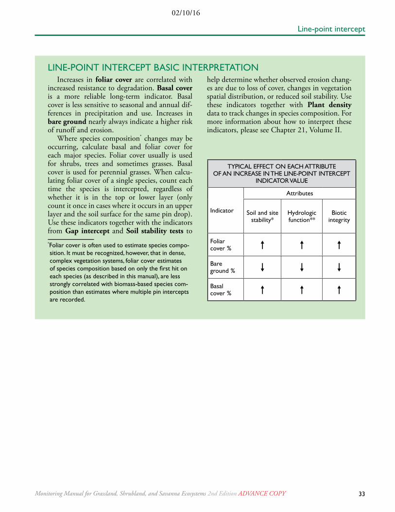
02/10/16
33Monitoring Manual for Grassland, Shrubland, and Savanna Ecosystems 2nd Edition AdvAncE copy
LINE-POINT INTERCEPT BASIC INTERPRETATION
Line-point intercept
Increases in foliar cover are correlated with increased resistance to degradation. Basal cover is a more reliable long-term indicator. Basal cover is less sensitive to seasonal and annual dif-ferences in precipitation and use. Increases in bare ground nearly always indicate a higher risk of runoff and erosion.
Where species composition* changes may be occurring, calculate basal and foliar cover for each major species. Foliar cover usually is used for shrubs, trees and sometimes grasses. Basal cover is used for perennial grasses. When calcu-lating foliar cover of a single species, count each time the species is intercepted, regardless of whether it is in the top or lower layer (only count it once in cases where it occurs in an upper layer and the soil surface for the same pin drop). Use these indicators together with the indicators from Gap intercept and Soil stability tests to *Foliar cover is often used to estimate species compo-sition. It must be recognized, however, that in dense, complex vegetation systems, foliar cover estimates of species composition based on only the first hit on each species (as described in this manual), are less strongly correlated with biomass-based species com-position than estimates where multiple pin intercepts are recorded.
help determine whether observed erosion chang-es are due to loss of cover, changes in vegetation spatial distribution, or reduced soil stability. Use these indicators together with Plant density data to track changes in species composition. For more information about how to interpret these indicators, please see Chapter 21, Volume II.
TyPICAL EFFECT ON EACH ATTRIBUTE OF AN INCREASE IN THE LINE-POINT INTERCEPT
INDICATOR VALUE
Indicator
Attributes
Soil and site stability*
Hydrologic function**
Biotic integrity
Foliar cover %
Bare ground %
Basal cover %
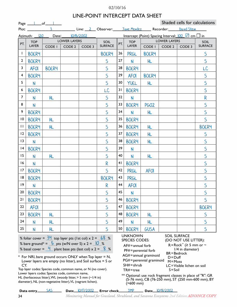
34 Monitoring Manual for Grassland, Shrubland, and Savanna Ecosystems 2nd Edition AdvAncE copy
02/10/16
Page 1 of 1
Plot: 3 Line: 2 Observer: Jane Mendez Recorder: David Stein
Azimuth: 120º Date: 10/15/2002 Intercept (Point) Spacing Interval: 100 ☑ cm ☐ in
PT. TOP LAyER
LOWER LAyERS SOIL SURFACE PT. TOP
LAyERLOWER LAyERS SOIL
SURFACECODE 1 CODE 2 CODE 3 CODE 1 CODE 2 CODE 3
1 BOER4 BOER4 26 PRGL BOER4 S2 BOER4 S 27 N HL S3 AF01 BOER4 S 28 BOER4 LC4 BOER4 S 29 AF01 BOER4 S5 N S 30 YUEL HL S6 BOER4 LC 31 BOER4 S7 N HL S 32 N R8 N S 33 BOER4 PG02 S9 BOER4 S 34 N HL S10 BOER4 HL S 35 BOER4 S11 BOER4 HL S 36 BOER4 HL BOER412 BOER4 S 37 BOER4 HL S13 N S 38 BOER4 HL S14 BOER4 S 39 N S15 N HL S 40 N HL S16 N R 41 BOER4 S17 BOER4 S 42 PRGL AF01 S18 BOER4 BOER4 43 PRGL S19 N R 44 AF01 S20 BOER4 S 45 N S21 BOER4 S 46 BOER4 S22 AF01 S 47 BOER4 BOER423 BOER4 HL S 48 BOER4 HL S24 N HL S 49 N HL S25 N HL S 50 BOER4 GUSA S
LINE-POINT INTERCEPT DATA SHEET
% foliar cover = 34 top layer pts (1st col) x 2 = 68 %% bare ground* = 5 pts (w/N over S) x 2 = 10 %% basal cover = 4 plant base pts (last col) x 2 = 8 %
Top layer codes: Species code, common name, or N (no cover).Lower layers codes: Species code, common name, HL (herbaceous litter), WL (woody litter, > 5 mm (~1/4 in) diameter), NL (non-vegetative litter), VL (vagrant lichen).
* For NRI, bare ground occurs ONLy when Top layer = N, Lower layers are empty (no litter), and Soil surface = S or Cy.
Shaded cells for calculations
UNKNOWN SPECIES CODES:AF#=annual forbPF#=perennial forb
AG#=annual graminoidPG#=perennial graminoidSH#=shrubTR#=tree
SOIL SURFACE (DO NOT USE LITTER):
R=Rock** (≥ 5 mm or ~1/4 in diameter)
BR=BedrockD=DuffM=Moss
LC=Visible lichen on soil S=Soil
** Optional: use rock fragment classes in place of "R": GR (5-76 mm), CB (76-250 mm), ST (250 mm-600 mm), By (>600 mm)
data entry SAS date 10/17/2002 Error check JMP date 10/18/2002
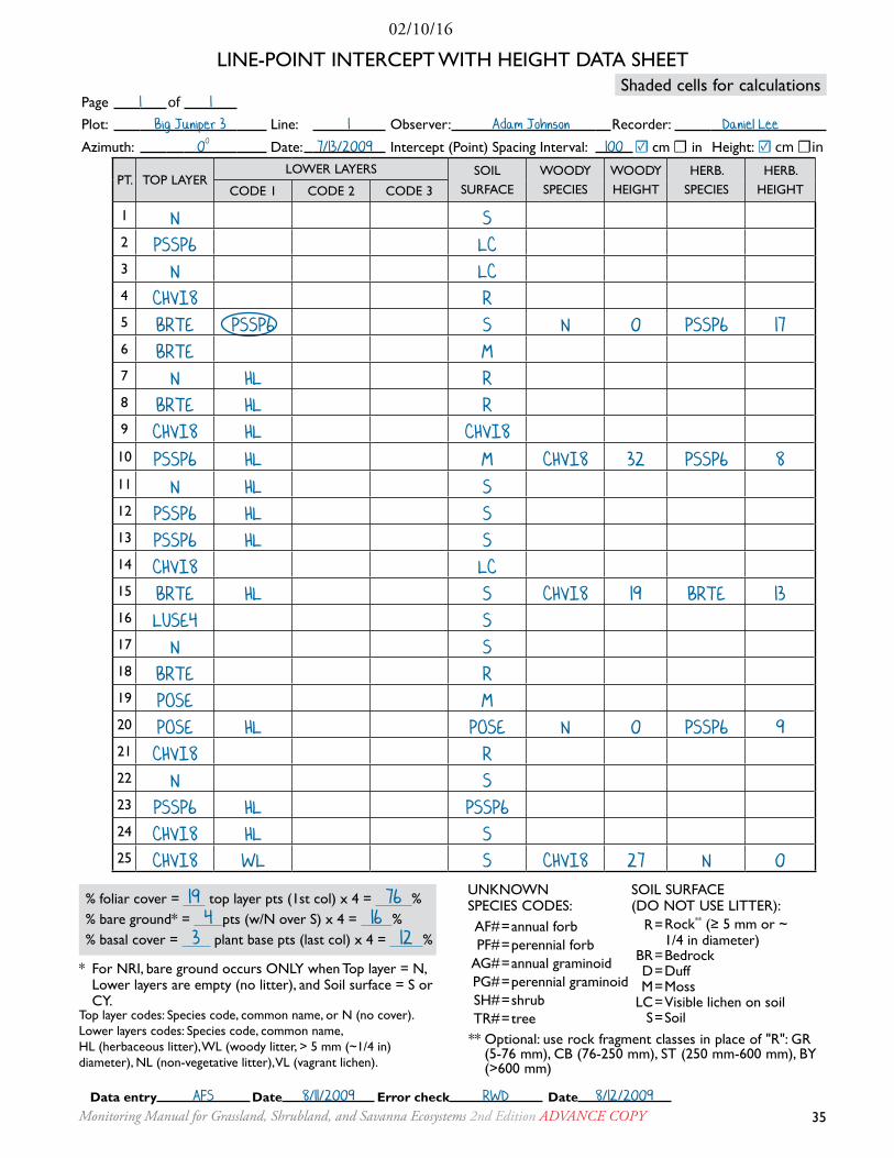
02/10/16
35Monitoring Manual for Grassland, Shrubland, and Savanna Ecosystems 2nd Edition AdvAncE copy
LINE-POINT INTERCEPT WITH HEIGHT DATA SHEET
% foliar cover = 19 top layer pts (1st col) x 4 = 76 %% bare ground* = 4 pts (w/N over S) x 4 = 16 %% basal cover = 3 plant base pts (last col) x 4 = 12 %
Top layer codes: Species code, common name, or N (no cover).Lower layers codes: Species code, common name, HL (herbaceous litter), WL (woody litter, > 5 mm (~1/4 in) diameter), NL (non-vegetative litter), VL (vagrant lichen).
* For NRI, bare ground occurs ONLy when Top layer = N, Lower layers are empty (no litter), and Soil surface = S or Cy.
Shaded cells for calculations
** Optional: use rock fragment classes in place of "R": GR (5-76 mm), CB (76-250 mm), ST (250 mm-600 mm), By (>600 mm)
UNKNOWN SPECIES CODES:AF#=annual forbPF#=perennial forb
AG#=annual graminoidPG#=perennial graminoidSH#=shrubTR#=tree
SOIL SURFACE (DO NOT USE LITTER):
R=Rock** (≥ 5 mm or ~1/4 in diameter)
BR=BedrockD=DuffM=Moss
LC=Visible lichen on soil S=Soil
PT. TOP LAyERLOWER LAyERS SOIL
SURFACEWOODy SPECIES
WOODy HEIGHT
HERB. SPECIES
HERB. HEIGHTCODE 1 CODE 2 CODE 3
1 N S2 PSSP6 LC3 N LC4 CHVI8 R5 BRTE PSSP6 S N 0 PSSP6 176 BRTE M7 N HL R8 BRTE HL R9 CHVI8 HL CHVI810 PSSP6 HL M CHVI8 32 PSSP6 811 N HL S12 PSSP6 HL S13 PSSP6 HL S14 CHVI8 LC15 BRTE HL S CHVI8 19 BRTE 1316 LUSE4 S17 N S18 BRTE R19 POSE M20 POSE HL POSE N 0 PSSP6 921 CHVI8 R22 N S23 PSSP6 HL PSSP624 CHVI8 HL S25 CHVI8 WL S CHVI8 27 N 0
Page 1 of 1
Plot: Big Juniper 3 Line: 1 Observer: Adam Johnson Recorder: Daniel Lee
Azimuth: 00 Date: 7/13/2009 Intercept (Point) Spacing Interval: 100 ☑ cm ☐ in Height: ☑ cm ☐in
data entry AFS date 8/11/2009 Error check RWD date 8/12/2009

36 Monitoring Manual for Grassland, Shrubland, and Savanna Ecosystems 2nd Edition AdvAncE copy
02/10/16
the tallest living or dead woody (including succulents) AND living or dead herbaceous plant parts intersecting a projected 30 cm (12 in) diameter cylinder tangent to the line (Figure 17).
1.2 All plant materials existing inside the pro-jected cylinder are considered, whether they are rooted inside or outside the 30 cm (12 in) circular area (Figure 18). It does not matter where plants are rooted, only plant materials within the cylinder are observed. I
1.3 Do not stretch or move any plant parts. Ig-nore any part of the plant that is outside the cylinder.
Vegetation height is measured as the height of the tallest plant part within a 30 cm (12 in) diameter cylinder projected tangent to the transect. It is mea-sured vertically from the soil surface at the center of the cylinder (Figure 17). Vegetation height provides plot-level vertical structure information necessary to predict soil erosion from wind and characterize wild-life habitat. Vegetation height is usually measured at the same time as Line-point intercept because it is more efficient, but can be measured separately.
MATERIALS• Measuring tape (length of transect)—if using
a tape measure in feet, use one marked in tenths of feet
• Two steel stakes for anchoring tape• Graduated survey rod or height measuring stick
with graduations in centimeters (or 0.5 in) and meters (or ft)
• 30 cm (12 in) diameter disc or ruler (optional)• Clinometer or extendable range pole• Electronic device for paperless data collection
(preferred) OR clipboard, Line-point Intercept with Height Data Sheet OR Vegetation Height Data Sheet (Appendix B) and pencil(s)
STANDARD METHODS (RULE SET) 1. Measure plant heights at regular intervals (5
m (10 ft) recommended) for a minimum of 28 height measurements per plot. Distribute the total number of height measurements evenly among all transects.
Rules1.1 At each designated transect mark, hold the
edge of the disc on the opposite side of the tape. Using the disc as a guide, determine
Figure 17. Measuring vegetation height.
7.5 m 10m
shrub
forb
5 m
30 cm
Figure 18. Example of vegetation height measurement intervals and the area tangent to the line in which the tallest woody and herbaceous plant elements are measured.
plant canopy (top-down view)
observer stands on this side
plant base
transect edge
VEGETATION HEIGHT

02/10/16
37Monitoring Manual for Grassland, Shrubland, and Savanna Ecosystems 2nd Edition AdvAncE copy
1.4 Height is determined as the perpendicular distance (relative to the earth's center, re-gardless of slope) from the soil surface at the center of the cylinder to the tallest plant ele-ment contained within the cylinder.
1.5 Record height from the center of the cylin-der at the soil surface, even if the soil surface is uneven, mounded or bumpy (Figure 19, Table 17). Woody or herbaceous litter are not measured.
2. Record the height of plants 0-2 m (6 ft) tall to the nearest centimeter (1 in). Record the height of plants that exceed 2 m (6 ft) in height to the nearest 30 cm (~1 ft). Plants greater than 18 m (60 ft) should be recorded as 18 m (60 ft) tall.
Rules2.1 Record the height of the tallest part of the
plant inside the cylinder. Record only one height for each plant type (woody or herba-ceous) if present. Where no woody or herba-ceous vegetation is present, mark "0" on the data sheet.
2.2 If vegetation is taller than 3 m (~10 ft), a clinometer, phone application, or geometric technique can be used to estimate height. For the geometric option, step back from the cylinder far enough so the tallest point of the plant in the cylinder can be seen. Measure (a) the horizontal distance to that point and (b) the angle (from the soil surface where the observer is standing) to that point. Calcu-late the height using the following formula: Height = (distance to plant) x (tangent of angle from soil surface). Be sure to measure and set calculators to ‘degrees’ when using this equation.
3. Record the plant species of each woody and her-baceous height measurement.
4. Optional: Record if the plant element is alive or dead.
Vegetation height
RipARiAn nOtE
No changes are needed for this method in riparian systems.
QUALitY AssURAnCE
☐ Each data sheet is complete. All points, observer, recorder, date, line, and plot name are recorded.
☐ Vegetation heights are collected at the correct intervals on the transect.
☐ Observers only measure plant elements within the cylinder tangent to the line.
☐ Species, if recorded, are included in the species list.
☐ Species names or codes are complete, correct and consistent with project plant coding system.
☐ Unknown plants are described according to unknown plant protocols, photographed and voucher specimens collected when permissible.
nRi
Record vegetation height separate from Line-point intercept. If data are recorded on paper data sheets, use the Vegetation Height Data Sheet (Appendix B) instead of the Line-point Intercept with Height Data Sheet.
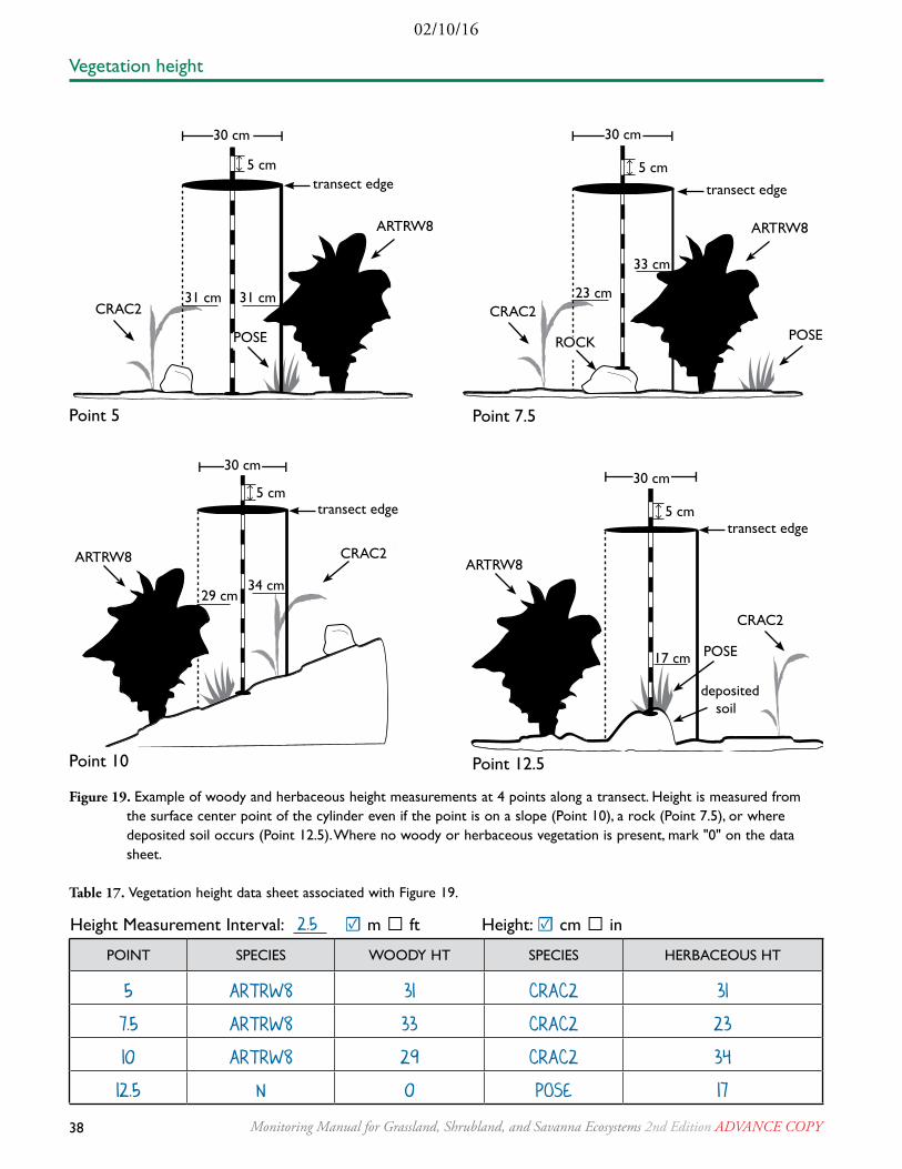
38 Monitoring Manual for Grassland, Shrubland, and Savanna Ecosystems 2nd Edition AdvAncE copy
02/10/16
Point 12.5
30 cm
CRAC2
POSE
deposited soil
ARTRW8
5 cmtransect edge
17 cm
Figure 19. Example of woody and herbaceous height measurements at 4 points along a transect. Height is measured from the surface center point of the cylinder even if the point is on a slope (Point 10), a rock (Point 7.5), or where deposited soil occurs (Point 12.5). Where no woody or herbaceous vegetation is present, mark "0" on the data sheet.
Table 17. Vegetation height data sheet associated with Figure 19.
POINT SPECIES WOODy HT SPECIES HERBACEOUS HT
5 ARTRW8 31 CRAC2 31
7.5 ARTRW8 33 CRAC2 23
10 ARTRW8 29 CRAC2 34
12.5 N 0 POSE 17
POSE
CRAC2
30 cm
Point 5
5 cmtransect edge
31 cm 31 cm
ARTRW8 ARTRW8
POSEROCK
30 cm
Point 7.5
5 cmtransect edge
23 cm
33 cm
CRAC2
CRAC2
Point 10
transect edge
29 cm34 cm
ARTRW8
5 cm
30 cm
Vegetation height
Height Measurement Interval: 2.5 ☑ m ☐ ft Height: ☑ cm ☐ in

02/10/16
39Monitoring Manual for Grassland, Shrubland, and Savanna Ecosystems 2nd Edition AdvAncE copy
VEGETATION HEIGHT INDICATOR CALCULATIONS
Vegetation height calculations are computed for two reasons: (1) to describe overall height structure on a plot and (2) to describe the heights of the veg-etation on the plot. Overall height structure on a plot, described in Steps 1, 2, and 3, is the average height recorded at all measurement intervals includ-ing measurements where no vegetation was present and height was recorded as "0". To describe the veg-etation height by structural group (woody or herba-ceous) or by species, average the heights recorded when those species or groups occur. Keep in mind that estimating vegetation height only where vegeta-tion was measured (height > 0) may result in variable number of height measurements between plots.
1. Calculate the average woody height for all mea-surements (woody vertical structure).
Rules1.1 Add together all woody species height values.
Divide this sum by the number of samples in this group. Record this value as the average woody height on your data sheet.
2. Calculate the average herbaceous height (herba-ceous vertical structure).
Rules2.1 Add together all herbaceous species height
measurements. Divide this sum by the num-ber of samples in this group. Record this value as average herbaceous height on your data sheet.
3. Calculate the average vegetation height (vertical structure) for all measurements. An example is shown in Table 18.
Rules3.1 Add together all height measurements, re-
gardless of species. Divide this sum by the number of samples in this group. Record this value as average overall height on your data sheet.
4. Optional: Calculate average of woody or herba-ceous heights including only heights > 0.
Table 18. Vegetation height data sheet example showing vegetation height measurements along a 25 m line and the resulting indicator calculations.
POINT SPECIES WOODy HT SPECIES HERBACEOUS HT
2.5 CHVI8 23 BRTE 8
5 ARTRW8 18 PSSP6 5
7.5 N 0 HECO26 22
10 ARTRW8 51 BRTE 23
12.5 CHVI8 28 N 0
15 CHVI8 27 BRTE 12
17.5 ARTRV 48 POSE 35
20 N 0 POSE 28
22.5 ARTRV 25 PSSP6 21
25 CHVI8 34 PSSP6 25
Vegetation height
Average vegetation height = 21.7 cm Average woody height = 25.4 cm Average herbaceous height = 17.9 cm
Height Measurement Interval: 2.5 ☑ m ☐ ft Height: ☑ cm ☐ in

40 Monitoring Manual for Grassland, Shrubland, and Savanna Ecosystems 2nd Edition AdvAncE copy
02/10/16
HABITAT TyPE
Breeding Brood-rearing Winter
SagebrushHeight (cm) 40-80 40-80 25-35
Canopy (%) 15-25 10-25 10-30
Forb/GrassHeight (cm) > 18 variable N/A
Canopy (%) ≥ 25 > 15 N/A
Table 19. Sage grouse canopy cover and vegetation height habitat requirements, adapted from Connelly et al. 2000**.
* Okin, G.S. 2008. A new model of wind erosion in the presence of vegetation. Journal of Geophysical Research 113: F02S10.
** Connelly, J.W., M.A. Schroeder, A.R. Sands, and C.E. Braun. 2000. Guidelines to manage sage grouse populations and their habitats. Wildlife Society Bulletin 28:967-985.
Woody and herbaceous height can be impor-tant indicators of vertical vegetation structure, especially when interpreted together with Gap intercept and Line-point intercept data. Woody and herbaceous vegetation structure, together with canopy gap size and distribution, are used to characterize wildlife habitat to determine if the site provides adequate thermal, hiding, and/or nesting cover for species of management interest (Table 19).
Vegetation height and canopy gaps are also
indicators of potential wind erosion on a site. A site with large canopy gaps and short vegetation is more susceptible to wind erosion than a site with smaller canopy gaps and taller vegetation. Models have been developed that predict wind erosion based on vegetation height, foliar cover and cano-py gaps (e.g., Okin 2008*). For more information about how to interpret these indicators, please see Volume II, Chapter 21.
VEGETATION HEIGHT BASIC INTERPRETATION
Vegetation height
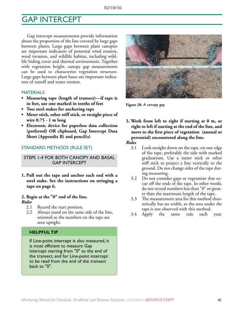
02/10/16
41Monitoring Manual for Grassland, Shrubland, and Savanna Ecosystems 2nd Edition AdvAncE copy
Gap intercept measurements provide information about the proportion of the line covered by large gaps between plants. Large gaps between plant canopies are important indicators of potential wind erosion, weed invasion, and wildlife habitat, including wild-life hiding cover and thermal environment. Together with vegetation height, canopy gap measurements can be used to characterize vegetation structure. Large gaps between plant bases are important indica-tors of runoff and water erosion.
MATERIALS• Measuring tape (length of transect)—if tape is
in feet, use one marked in tenths of feet• Two steel stakes for anchoring tape• Meter stick, other stiff stick, or straight piece of
wire 0.75 - 1 m long• Electronic device for paperless data collection
(preferred) OR clipboard, Gap Intercept Data Sheet (Appendix B) and pencil(s)
STANDARD METHODS (RULE SET)
1. Pull out the tape and anchor each end with a steel stake. See the instructions on stringing a tape on page 6.
2. Begin at the "0" end of the line.Rules
2.1 Record the start position. 2.2 Always stand on the same side of the line,
oriented so the numbers on the tape are seen upright.
3. Work from left to right if starting at 0 m, or right to left if starting at the end of the line, and move to the first piece of vegetation (annual or perennial) encountered along the line.
Rules3.1 Look straight down on the tape, on one edge
of the tape, preferably the side with marked graduations. Use a meter stick or other stiff stick to project a line vertically to the ground. Do not change sides of the tape dur-ing measuring.
3.2 Do not consider gaps or vegetation that oc-cur off the ends of the tape. In other words, do not record numbers less than "0" or great-er than the maximum length of the tape.
3.3 The measurement area for this method theo-retically has no width, so the area under the tape is not observed with this method.
3.4 Apply the same rule each year.
Figure 20. A canopy gap.
GAP INTERCEPT
STEPS 1-4 FOR BOTH CANOPy AND BASAL GAP INTERCEPT
HELpfUL tip
If Line-point intercept is also measured, it is most efficient to measure Gap intercept starting from "0" to the end of the transect, and for Line-point intercept to be read from the end of the transect back to "0".
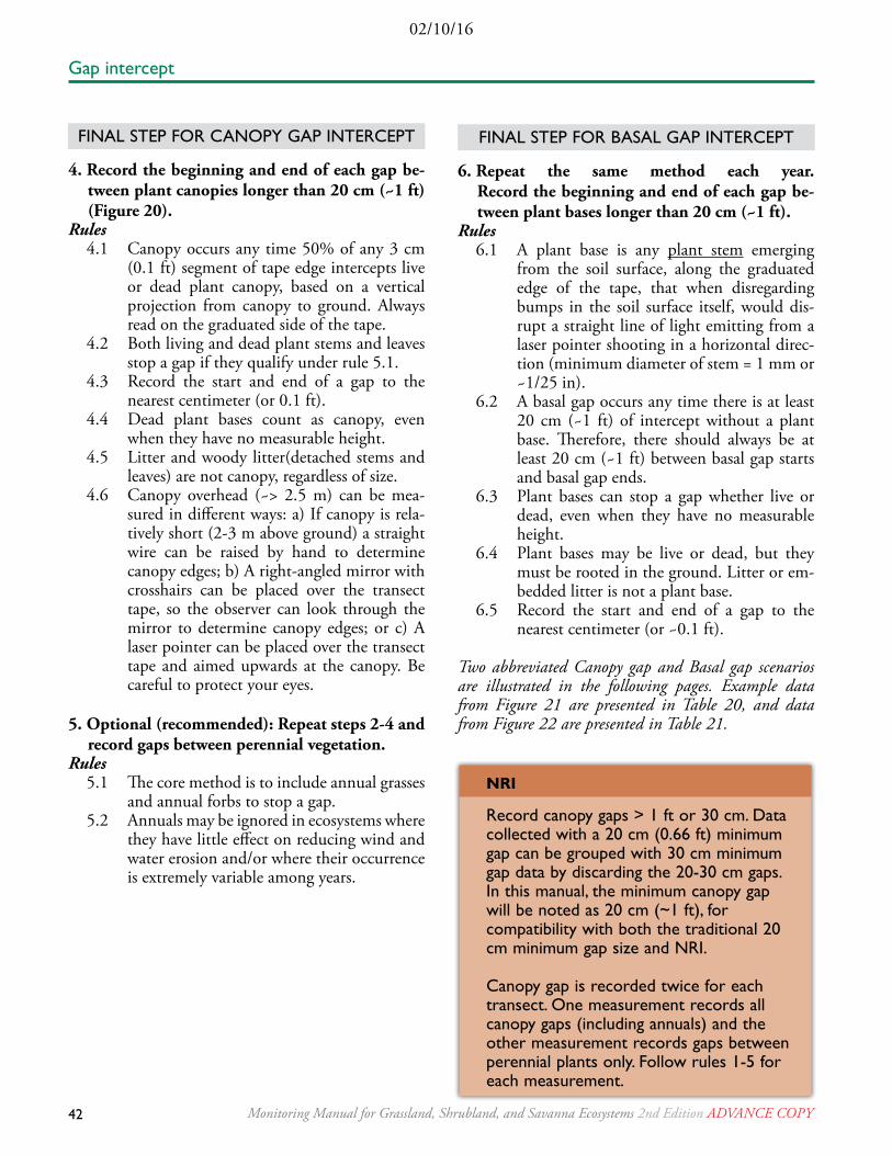
42 Monitoring Manual for Grassland, Shrubland, and Savanna Ecosystems 2nd Edition AdvAncE copy
02/10/16
4. Record the beginning and end of each gap be-tween plant canopies longer than 20 cm (~1 ft) (Figure 20).
Rules4.1 Canopy occurs any time 50% of any 3 cm
(0.1 ft) segment of tape edge intercepts live or dead plant canopy, based on a vertical projection from canopy to ground. Always read on the graduated side of the tape.
4.2 Both living and dead plant stems and leaves stop a gap if they qualify under rule 5.1.
4.3 Record the start and end of a gap to the nearest centimeter (or 0.1 ft).
4.4 Dead plant bases count as canopy, even when they have no measurable height.
4.5 Litter and woody litter(detached stems and leaves) are not canopy, regardless of size.
4.6 Canopy overhead (~> 2.5 m) can be mea-sured in different ways: a) If canopy is rela-tively short (2-3 m above ground) a straight wire can be raised by hand to determine canopy edges; b) A right-angled mirror with crosshairs can be placed over the transect tape, so the observer can look through the mirror to determine canopy edges; or c) A laser pointer can be placed over the transect tape and aimed upwards at the canopy. Be careful to protect your eyes.
5. Optional (recommended): Repeat steps 2-4 and record gaps between perennial vegetation.
Rules5.1 The core method is to include annual grasses
and annual forbs to stop a gap.5.2 Annuals may be ignored in ecosystems where
they have little effect on reducing wind and water erosion and/or where their occurrence is extremely variable among years.
6. Repeat the same method each year. Record the beginning and end of each gap be-tween plant bases longer than 20 cm (~1 ft).
Rules6.1 A plant base is any plant stem emerging
from the soil surface, along the graduated edge of the tape, that when disregarding bumps in the soil surface itself, would dis-rupt a straight line of light emitting from a laser pointer shooting in a horizontal direc-tion (minimum diameter of stem = 1 mm or ~1/25 in).
6.2 A basal gap occurs any time there is at least 20 cm (~1 ft) of intercept without a plant base. Therefore, there should always be at least 20 cm (~1 ft) between basal gap starts and basal gap ends.
6.3 Plant bases can stop a gap whether live or dead, even when they have no measurable height.
6.4 Plant bases may be live or dead, but they must be rooted in the ground. Litter or em-bedded litter is not a plant base.
6.5 Record the start and end of a gap to the nearest centimeter (or ~0.1 ft).
Two abbreviated Canopy gap and Basal gap scenarios are illustrated in the following pages. Example data from Figure 21 are presented in Table 20, and data from Figure 22 are presented in Table 21.
Gap intercept
FINAL STEP FOR CANOPy GAP INTERCEPT
nRi
Record canopy gaps > 1 ft or 30 cm. Data collected with a 20 cm (0.66 ft) minimum gap can be grouped with 30 cm minimum gap data by discarding the 20-30 cm gaps. In this manual, the minimum canopy gap will be noted as 20 cm (~1 ft), for compatibility with both the traditional 20 cm minimum gap size and NRI.
Canopy gap is recorded twice for each transect. One measurement records all canopy gaps (including annuals) and the other measurement records gaps between perennial plants only. Follow rules 1-5 for each measurement.
FINAL STEP FOR BASAL GAP INTERCEPT
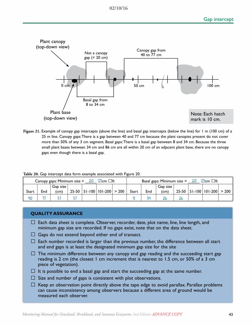
02/10/16
43Monitoring Manual for Grassland, Shrubland, and Savanna Ecosystems 2nd Edition AdvAncE copy
Gap intercept
Figure 21. Example of canopy gap intercepts (above the line) and basal gap intercepts (below the line) for 1 m (100 cm) of a 25 m line. Canopy gaps: There is a gap between 40 and 77 cm because the plant canopies present do not cover more than 50% of any 3 cm segment. Basal gaps: There is a basal gap between 8 and 34 cm. Because the three small plant bases between 34 cm and 86 cm are all within 20 cm of an adjacent plant base, there are no canopy gaps even though there is a basal gap.
Not a canopy gap (< 20 cm)
Basal gap from8 to 34 cm
Canopy gap from40 to 77 cm
100 cm
Plant canopy (top-down view)
Plant base (top-down view)
0 cm 50 cm
Note: Each hatch mark is 10 cm.
Canopy gaps: Minimum size = _____ ☑cm ☐ft Basal gaps: Minimum size = _____ ☑cm ☐ft
Start EndGap size
(cm) 25-50 51-100 101-200 > 200 Start EndGap size
(cm) 25-50 51-100 101-200 > 200
40 77 37 37 8 34 26 26
Table 20. Gap intercept data form example associated with Figure 20.
QUALitY AssURAnCE
☐ Each data sheet is complete. Observer, recorder, date, plot name, line, line length, and minimum gap size are recorded. If no gaps exist, note that on the data sheet.
☐ Gaps do not extend beyond either end of transect. ☐ Each number recorded is larger than the previous number, the difference between all start and end gaps is at least the designated minimum gap size for the site
☐ The minimum difference between any canopy end gap reading and the succeeding start gap reading is 2 cm (the closest 1 cm increment that is nearest to 1.5 cm, or 50% of a 3 cm piece of vegetation).
☐ It is possible to end a basal gap and start the succeeding gap at the same number. ☐ Size and number of gaps is consistent with plot observations. ☐ Keep an observation point directly above the tape edge to avoid parallax. Parallax problems can cause inconsistency among observers because a different area of ground would be measured each observer.
20 20
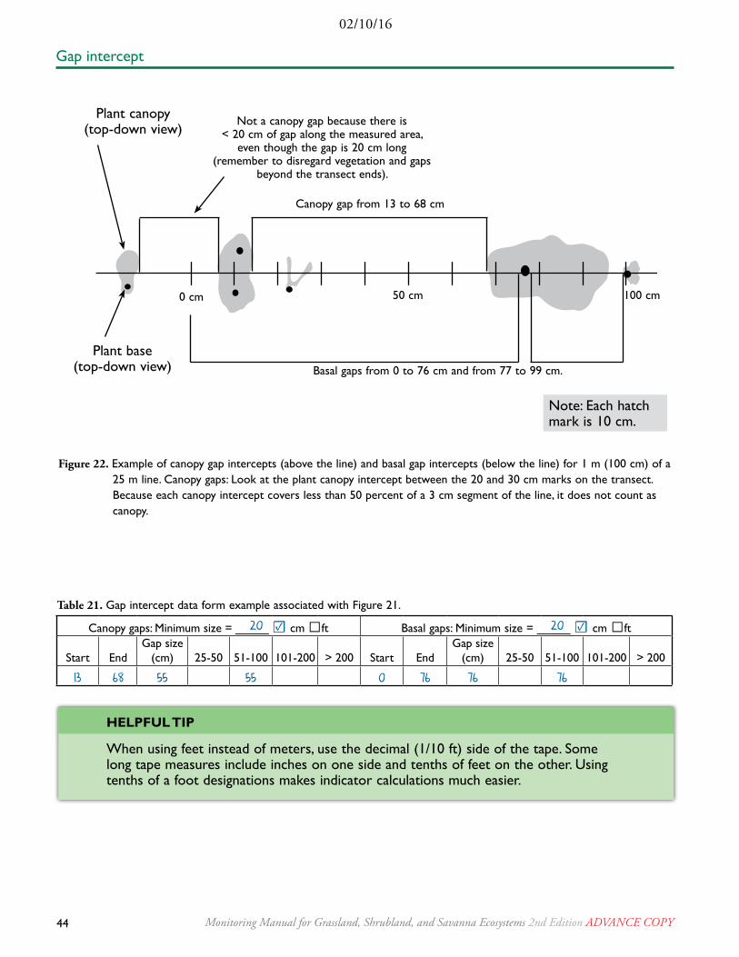
44 Monitoring Manual for Grassland, Shrubland, and Savanna Ecosystems 2nd Edition AdvAncE copy
02/10/16
Figure 22. Example of canopy gap intercepts (above the line) and basal gap intercepts (below the line) for 1 m (100 cm) of a 25 m line. Canopy gaps: Look at the plant canopy intercept between the 20 and 30 cm marks on the transect. Because each canopy intercept covers less than 50 percent of a 3 cm segment of the line, it does not count as canopy.
Basal gaps from 0 to 76 cm and from 77 to 99 cm.
0 cm 100 cm
Not a canopy gap because there is < 20 cm of gap along the measured area,
even though the gap is 20 cm long (remember to disregard vegetation and gaps
beyond the transect ends).
Plant canopy (top-down view)
Plant base (top-down view)
50 cm
Canopy gap from 13 to 68 cm
Table 21. Gap intercept data form example associated with Figure 21.
Gap intercept
Note: Each hatch mark is 10 cm.
Canopy gaps: Minimum size = _____ ☑ cm ☐ft Basal gaps: Minimum size = _____ ☑ cm ☐ft
Start EndGap size
(cm) 25-50 51-100 101-200 > 200 Start EndGap size
(cm) 25-50 51-100 101-200 > 200
13 68 55 55 0 76 76 76
20 20
HELpfUL tip
When using feet instead of meters, use the decimal (1/10 ft) side of the tape. Some long tape measures include inches on one side and tenths of feet on the other. Using tenths of a foot designations makes indicator calculations much easier.

02/10/16
45Monitoring Manual for Grassland, Shrubland, and Savanna Ecosystems 2nd Edition AdvAncE copy
Circle one: includes only perennial vegetation OR includes annual and perennial vegetation
Canopy gaps: Minimum size = _____ ☑cm ☐ft Basal gaps: Minimum size = _____ ☑cm ☐ft
Start(cm/ft)
End(cm/ft)
Gap (cm) size (ft)
25-50 51-100 101-200 > 200 Start(cm/ft)
End(cm/ft)
Gap (cm) size (ft)
25-50 51-100 101-200 > 2001-2 2.1-3 3.1-6 > 6 1-2 2.1-3 3.1-6 > 6
40 60 20 27 64 37 37
101 202 101 101 70 264 194 194
237 963 726 726 269 459 190 190
4704 4754 50 50 3560 4684 1124 1124
4761 4925 164 164 4720 4813 93 93
4931 5000 69 69 4817 5000 183 183
SUM (cm/ft) 50 69 265 726 SUM (cm/ft) 37 93 567 1124
LINE LENGTH (cm/ft) 5000 5000 5000 5000 LINE LENGTH (cm/ft) 5000 5000 5000 5000
SUM ÷ LINE LENGTH 0.01 0.014 0.053 0.145 SUM ÷ LINE LENGTH 0.007 0.019 0.113 0.225
x 100 x 100 x 100 x 100 x 100 x 100 x 100 x 100
% of line in gaps 1.0% 1.4% 5.3% 14.5% % of line in gaps 0.7% 1.9% 11.3% 22.5%
Gap intercept
GAP INTERCEPT INDICATOR CALCULATIONS
1. Canopy gaps: Calculate the percentage of the line covered in gaps 25-50* cm (optional), 51-100 cm, 101-200 cm and greater than 200 cm long (Table 22).
Rules1.1 Calculate each Gap size in centimeters (Gap
end minus Gap start) for each canopy gap entered on the data sheet.
1.2 If a gap is 25-50 cm long, record its “Gap size” (cm) under the “25-50” column. Re-peat this for all gaps for the remaining size classes (51-100, 101-200 and > 200).
1.3 Add the gaps for each shaded column and re-cord this value next to “SUM” at the bottom of the column. This is the total amount of the line (in centimeters) covered by gaps in size classes 25-50, 51-100, 101-200, and > 200 cm. Record the “LINE LENGTH” in centime-ters on the data sheet. Line length in centi-meters is equal to the length of the line (in meters) multiplied by 100.
*20 cm minimum gap sizes are more easily distinguished in the field, but reporting of gap sizes traditionally begins with gaps >25 cm.
1.4 Starting with the gaps 25-50 cm, divide the “SUM” by the “LINE LENGTH” and mul-tiply this value by 100 to obtain the percent of the line covered in gaps 25-50 cm. Record this value under the appropriate column next to “% of line in gaps”. Repeat this for gaps 51-100, 101-200, and > 200 cm.
2. Basal gaps: Calculate the percentage of the line covered in gaps 25-50 cm, 51-100 cm, 101-200 cm, and greater than 200 cm long (Table 22).
Rules2.1 Follow steps 1.1 through 1.5 above for basal
gaps.
3. Optional for canopy and basal gaps: Use a dif-ferent color or pattern to mark a slice of the pie chart for each gap’s size class. The dark blue sec-tion represents the area covered by plants and gaps less than 25 cm (Figure 23).
Table 22. Gap intercept data form example showing part of a 50 m line and associated indicator calculations.
20 20

46 Monitoring Manual for Grassland, Shrubland, and Savanna Ecosystems 2nd Edition AdvAncE copy
02/10/16
1% 25-50 cm
1.4%51-100 cm
77.8 %in canopy and/or in canopy gaps
smaller than 25 cm
61.6% in plantbases and/or in basal
gaps smaller than 25 cm
14.5%> 200 cm
5.3%101-200 cm
0.7% 25-50 cm
1.9%51-100 cm 11.3%
101-200 cm
24.5%> 200 cm
Canopy Gap Pie Chart Basal Gap Pie Chart
Figure 23. Examples of how to present gap intercept data in pie charts. Size of each pie slice is proportional to the area cov-ered by each type of gap.
Gap intercept
GAP INTERCEPT BASIC INTERPRETATION
Increases in the proportion of the line covered by canopy gaps are related to increased risk of wind erosion. For example, wind velocities in most areas of the western United States are capa-ble of moving loose, disturbed soil in 50 cm (20 in) gaps in grasslands. Disturbed soil in gaps 1-2 m (3-6 ft) in diameter is nearly as susceptible to wind erosion as soil with no vegetation cover (all gap). Minimum gap size required to cause wind erosion increases with vegetation height.
Increases in the proportion of the line covered by large basal gaps reflect increased susceptibility to water erosion and runoff. Plant bases slow water movement down slopes. As basal gap sizes increase, there are fewer obstacles to slow water flow, so runoff and erosion increase. Increases in the size of large basal gaps have a greater effect where rock and litter cover are low, since they are the only obstacles to water flow and erosion.
Use these indicators together with the cover indicators from Line-point intercept and the soil
structure indicators from Soil stability tests to help determine whether observed erosion chang-es are due to loss of cover, changes in spatial dis-tribution of vegetation, or reduced soil stability.
Where gaps are approximately circular, typical gap diameter is approximately 1.3 times the gap intercept. For more information about how to interpret these indicators, please see Volume II, Chapter 21.
TyPICAL EFFECT ON EACH ATTRIBUTE OF AN INCREASE IN THE LINE-POINT INTERCEPT
INDICATOR VALUE
Indicator
Attributes
Soil and site stability
Hydrologic function
Biotic integrity
Canopy gaps (%) i i iBasal gaps (%) i i i
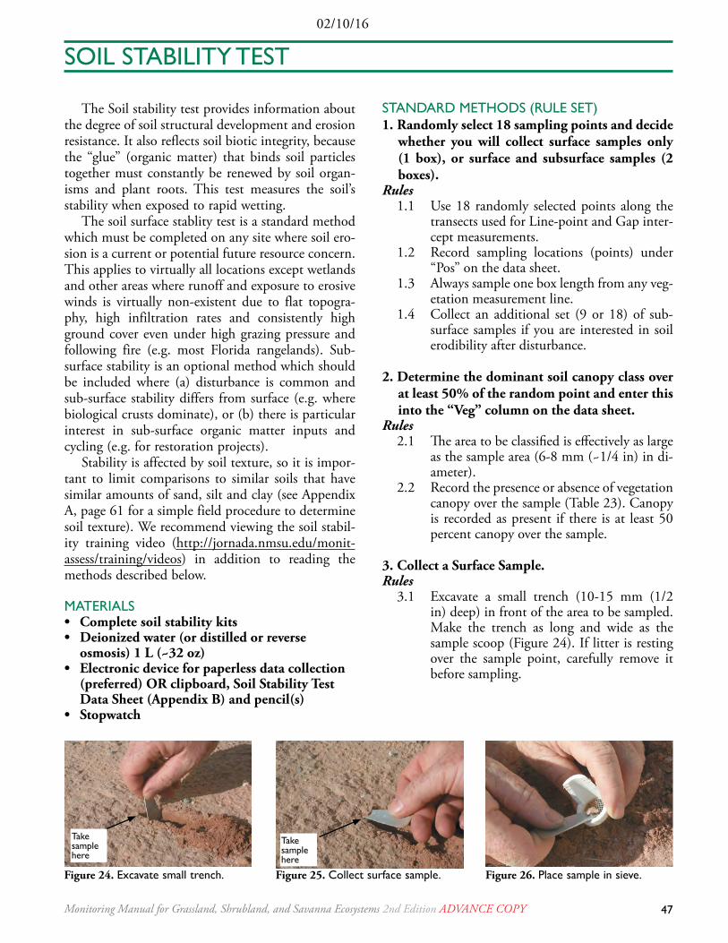
02/10/16
47Monitoring Manual for Grassland, Shrubland, and Savanna Ecosystems 2nd Edition AdvAncE copy
The Soil stability test provides information about the degree of soil structural development and erosion resistance. It also reflects soil biotic integrity, because the “glue” (organic matter) that binds soil particles together must constantly be renewed by soil organ-isms and plant roots. This test measures the soil’s stability when exposed to rapid wetting.
The soil surface stablity test is a standard method which must be completed on any site where soil ero-sion is a current or potential future resource concern. This applies to virtually all locations except wetlands and other areas where runoff and exposure to erosive winds is virtually non-existent due to flat topogra-phy, high infiltration rates and consistently high ground cover even under high grazing pressure and following fire (e.g. most Florida rangelands). Sub-surface stability is an optional method which should be included where (a) disturbance is common and sub-surface stability differs from surface (e.g. where biological crusts dominate), or (b) there is particular interest in sub-surface organic matter inputs and cycling (e.g. for restoration projects).
Stability is affected by soil texture, so it is impor-tant to limit comparisons to similar soils that have similar amounts of sand, silt and clay (see Appendix A, page 61 for a simple field procedure to determine soil texture). We recommend viewing the soil stabil-ity training video (http://jornada.nmsu.edu/monit-assess/training/videos) in addition to reading the methods described below.
MATERIALS• Complete soil stability kits• Deionizedwater(ordistilledorreverse
osmosis) 1 L (~32 oz)• Electronicdeviceforpaperlessdatacollection
(preferred) OR clipboard, Soil Stability Test Data Sheet (Appendix B) and pencil(s)
• Stopwatch
Figure 24. Excavate small trench.
Take sample here
Take sample here
Figure 25. Collect surface sample. Figure 26. Place sample in sieve.
STANDARD METHODS (RULE SET) 1. Randomly select 18 sampling points and decide
whether you will collect surface samples only (1 box), or surface and subsurface samples (2 boxes).
Rules1.1 Use 18 randomly selected points along the
transects used for Line-point and Gap inter-cept measurements.
1.2 Record sampling locations (points) under “Pos” on the data sheet.
1.3 Always sample one box length from any veg-etation measurement line.
1.4 Collect an additional set (9 or 18) of sub-surface samples if you are interested in soil erodibility after disturbance.
2. Determine the dominant soil canopy class over at least 50% of the random point and enter this into the “Veg” column on the data sheet.
Rules2.1 The area to be classified is effectively as large
as the sample area (6-8 mm (~1/4 in) in di-ameter).
2.2 Record the presence or absence of vegetation canopy over the sample (Table 23). Canopy is recorded as present if there is at least 50 percent canopy over the sample.
3. Collect a Surface Sample.Rules
3.1 Excavate a small trench (10-15 mm (1/2 in) deep) in front of the area to be sampled. Make the trench as long and wide as the sample scoop (Figure 24). If litter is resting over the sample point, carefully remove it before sampling.
SOIL STABILITy TEST

48 Monitoring Manual for Grassland, Shrubland, and Savanna Ecosystems 2nd Edition AdvAncE copy
02/10/16
Figure 27. Ensure correct sample size.
3.2 Gently push the sample scoop horizontally into the 10-15 mm deep exposed vertical face of the small trench, lift out a soil frag-ment and trim it (if necessary) to the correct size (Figure 25).
3.3 The soil fragment needs to be 2-3 mm (< 1/8 in) thick and 6-8 mm (1/4 in) in diameter (Figures 27, 28, and 29). This is the diameter of a wood pencil eraser. Try to fit sample in this dot (6-8 mm diameter).
3.4 Collect samples at the exact point. Move the sample point only if it has been disturbed during previous measure-ments or the soil surface is protected by a rock or embedded litter. Move the point a standard distance (e.g., 15 cm, 0.5 ft) and note this change on the data sheet.
3.5 Minimize shattering by: a) slicing the soil around the sample before lifting; b) lifting
SOIL COVER CODE ACTION
No perennial plant canopy (e.g., annuals and lichens)
nC=No cover
Sample (see Rules 3.6-3.8 for additional guidance)Perennial
plant canopy
C=Cover ----------OR----------g = perennial grass canopy and grass/shrub canopy mixturef = perennial forbsh = shrub canopyt = Tree Canopy
Root mat MossDuff Water
M = "root mat"
Do not sample, record a stability value of "6"
Rock fragment (gravel, cobble, stone, boulder, bedrock)
No data recorded
Move a standard distance away and attempt to sample again(see Rule 3.4)
Table 23. Record the soil canopy cover code for each soil sample point. For some canopy covers, no soil sample is collected and a value of "6" is recorded on the data sheet.
Figure 28. Samples are 2-3 mm (<1/8 in) thick.
Soil stability test
RipARiAn nOtE
No changes are needed for this method in riparian systems.

02/10/16
49Monitoring Manual for Grassland, Shrubland, and Savanna Ecosystems 2nd Edition AdvAncE copy
out a slightly larger sample than required, and trimming it to size in the palm of your hand; and/or c) misting the sample area be-fore collection (see 3.6).
3.6 If the soil sample is too weakly structured to sample (falls through the sieve), mist it light-ly with deionized water (use an atomizer or equivalent) and then take a sample. Perfume and plastic hair spray bottles work well for this. If the sample still will not hold togeth-er, record a “1” on the data sheet. Do not as-sume that a soil is unstable before spraying. Coarse textured soils and disturbed surfaces may appear unstable when dry but could be stable when wet.
3.7 If the soil surface is covered by a lichen or visibly darkened cyanobacterial crust, in-clude the crust in the sample. Roots may also be included in the sample.
3.8 If the sample mark falls on a plant base, col-lect the sample from within the plant base when feasible, otherwise sample as close as possible to the plant base.
3.9 Gently place the sample upright in a dry sieve (Figures 26, 27, 32); place sieve in the appropriate cell of a dry box (Figure 31). Leave box lid open (Figure 31).
4. Optional: collect a subsurface sample (see Step 1).
Rules4.1 Sample directly below the surface sample.4.2 Use the flat, square (handle) end of the
scoop to gently excavate the previous trench (in front of the surface sample) to a depth of 40-50 mm (1 1/2 - 2 in).
4.3 Directly below the surface sample, remove soil so that a “shelf ” is created with the top step 25 mm (1 in) below the soil surface (Figure 30).
4.4 Use the scoop to lift out a subsurface sample from below (Figure 30).
4.5 The soil fragment must be 2-3 mm (< 1/8 in) thick and 6-8 mm (1/4 in) in diameter (Figures 28 and 30).
4.6 See steps 3.5-3.6. If you encounter a rock, record “R” and move to the next sample.
4.7 Place the sample upright in a dry sieve; place sieve in appropriate cell of a dry box. Leave box lid open (Figure 32).
2-3 mm
25 mm
Figure 29. Excavate trench for subsurface sample
Figure 30. Collect subsurface sample.
Figure 31. Sample in sieve, drawn to scale. Sample shape may vary from round to square to slightly irregular as shown above.
Soil stability test
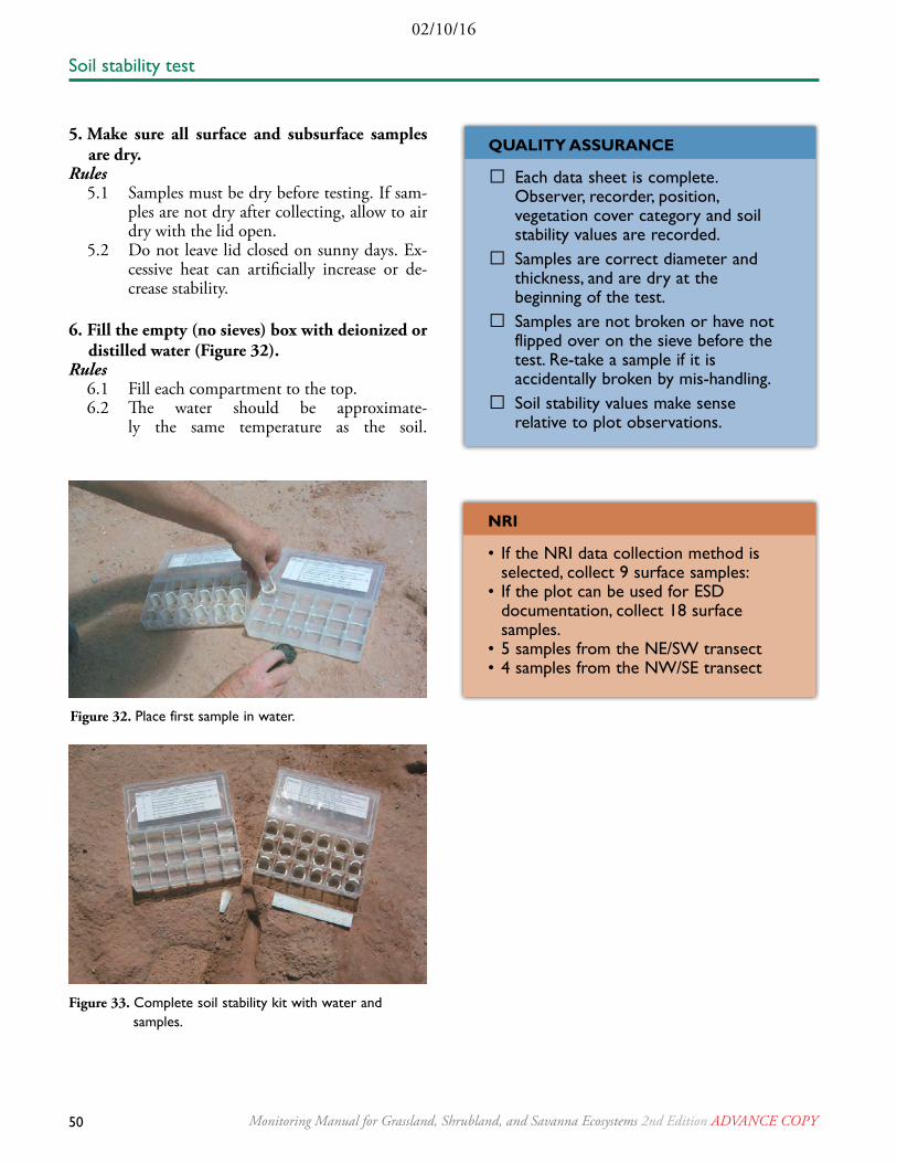
50 Monitoring Manual for Grassland, Shrubland, and Savanna Ecosystems 2nd Edition AdvAncE copy
02/10/16
Soil stability test
5. Make sure all surface and subsurface samples are dry.
Rules5.1 Samples must be dry before testing. If sam-
ples are not dry after collecting, allow to air dry with the lid open.
5.2 Do not leave lid closed on sunny days. Ex-cessive heat can artificially increase or de-crease stability.
6. Fill the empty (no sieves) box with deionized or distilled water (Figure 32).
Rules6.1 Fill each compartment to the top.6.2 The water should be approximate-
ly the same temperature as the soil.
Figure 32. Place first sample in water.
Figure 33. Complete soil stability kit with water and samples.
QUALitY AssURAnCE
☐ Each data sheet is complete. Observer, recorder, position, vegetation cover category and soil stability values are recorded.
☐ Samples are correct diameter and thickness, and are dry at the beginning of the test.
☐ Samples are not broken or have not flipped over on the sieve before the test. Re-take a sample if it is accidentally broken by mis-handling.
☐ Soil stability values make sense relative to plot observations.
nRi
• If the NRI data collection method is selected, collect 9 surface samples:
• If the plot can be used for ESD documentation, collect 18 surface samples.
• 5 samples from the NE/SW transect • 4 samples from the NW/SE transect

02/10/16
51Monitoring Manual for Grassland, Shrubland, and Savanna Ecosystems 2nd Edition AdvAncE copy
Soil stability test
Stability class
Criteria for assignment to stability class
1 50% of structural integrity lost (melts) within 5 seconds of immersion in water, And < 10% remains after 5 dipping cycles, OR soil too unstable to sample (falls through sieve).
2 50% of structural integrity lost (melts) 5-30 seconds after immersion And < 10% remains after 5 dipping cycles.
3 50% of structural integrity lost (melts) 30-300 seconds after immersion, OR < 10% of soil remains on the sieve after five dipping cycles.
4 10–25% of soil remains on the sieve after five dipping cycles.
5 25–75% of soil remains on the sieve after five dipping cycles.
6 75–100% of soil remains on the sieve after five dipping cycles.
Table 24. Stability class ratings. Percent soil remaining on the sieve for stability classes 4-6 refers to the percentage of the total volume remaining for the original size of the sample before immersion. See Figure 34 for photos illustrating stability classes 1, 4, 5 and 6.
7. Test the samples.Rules
7.1 Lower the first sieve with the sample into the respective water-filled compartment—upper left corner of sample box to upper left corner of water box (Figure 32).
7.2 From the time the sieve screen touches the water surface to the time it rests on the bot-tom of the box, 1 second should elapse.
7.3 Start the stopwatch when the first sample touches the water. Use Table 24 to assign samples to stability classes.
7.4 Follow the sequence of immersions on the data sheet, adding one sample every 15 sec-onds, requiring a total of 10 minutes for 18 samples. Beginners may want to immerse a sample every 30 seconds, and then dip sam-ples at 30 second intervals. This allows nine samples to be run in 10 minutes, or 20 min-utes to test one box of 18 samples
7.5 Observe the fragments from the time the sample hits the water until 5 minutes (300 seconds) has elapsed, then assign a stability class based on Table 24.
7.6 After 5 minutes has elapsed for each sample, in sequence, raise each sieve completely out of the water and then lower it to the bottom without touching the bottom of the tray. Re-peat this immersion and dipping a total of five times for each sieve. Do this even if you have already rated the sample a 1, 2 or 3 (it is possible to increase the rating if after siev-ing, > 10% of soil remains on sieve). Assign a stability class based on Table 24.
7.7 For the dipping rate, it should take 1 second for each sieve to clear the water’s surface and 1 second to return to near the bottom of the box. The process is strictly timed so dipping 5 times takes 10 seconds, allowing an addi-tional 5 seconds to write the value on the data sheet before processing the next sample.
7.8 Hydrophobic samples (float in water after attempting to push under) are rated 6 and circled on the data sheet.
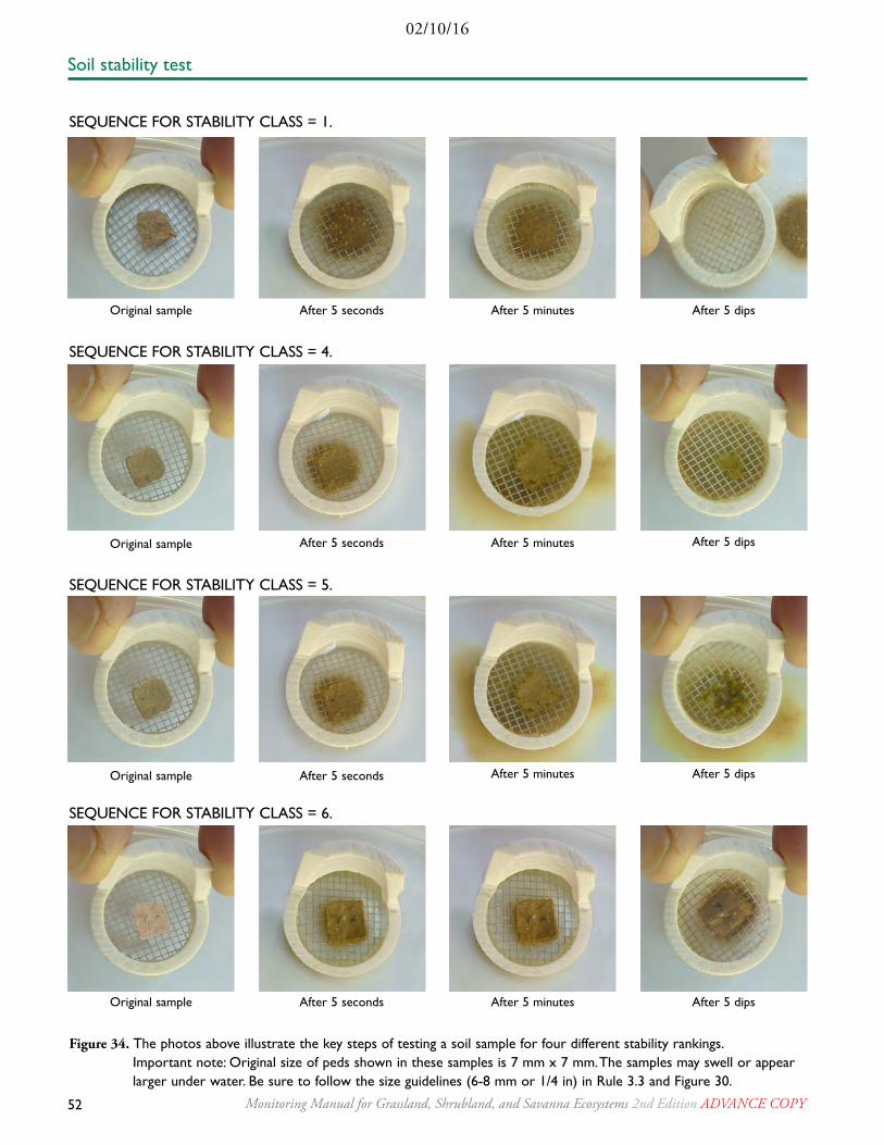
52 Monitoring Manual for Grassland, Shrubland, and Savanna Ecosystems 2nd Edition AdvAncE copy
02/10/16
Figure 34. The photos above illustrate the key steps of testing a soil sample for four different stability rankings. Important note: Original size of peds shown in these samples is 7 mm x 7 mm. The samples may swell or appear larger under water. Be sure to follow the size guidelines (6-8 mm or 1/4 in) in Rule 3.3 and Figure 30.
SEQUENCE FOR STABILITy CLASS = 1.
SEQUENCE FOR STABILITy CLASS = 4.
SEQUENCE FOR STABILITy CLASS = 5.
SEQUENCE FOR STABILITy CLASS = 6.
Original sample
Original sample
Original sample
Original sample
After 5 seconds
After 5 seconds
After 5 seconds
After 5 seconds
After 5 minutes
After 5 minutes
After 5 minutes
After 5 minutes
After 5 dips
After 5 dips
After 5 dips
After 5 dips
Soil stability test
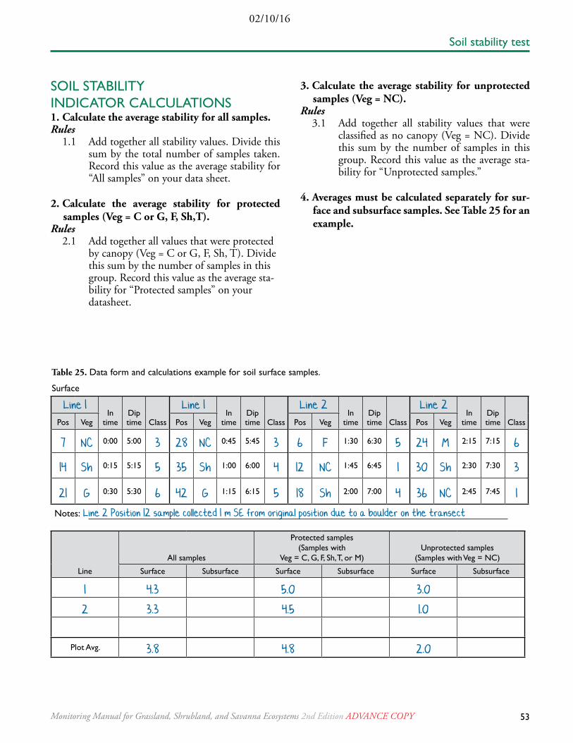
02/10/16
53Monitoring Manual for Grassland, Shrubland, and Savanna Ecosystems 2nd Edition AdvAncE copy
Table 25. Data form and calculations example for soil surface samples.
SOIL STABILITy INDICATOR CALCULATIONS1. Calculate the average stability for all samples.Rules
1.1 Add together all stability values. Divide this sum by the total number of samples taken. Record this value as the average stability for “All samples” on your data sheet.
2. Calculate the average stability for protected samples (Veg = C or G, F, Sh,T).
Rules2.1 Add together all values that were protected
by canopy (Veg = C or G, F, Sh, T). Divide this sum by the number of samples in this group. Record this value as the average sta-bility for “Protected samples” on your datasheet.
3. Calculate the average stability for unprotected samples (Veg = NC).
Rules3.1 Add together all stability values that were
classified as no canopy (Veg = NC). Divide this sum by the number of samples in this group. Record this value as the average sta-bility for “Unprotected samples.”
4. Averages must be calculated separately for sur-face and subsurface samples. See Table 25 for an example.
Surface
Line 1In
timeDip time Class
Line 1In
timeDip time Class
Line 2In
timeDip time Class
Line 2In
timeDip time ClassPos Veg Pos Veg Pos Veg Pos Veg
7 NC 0:00 5:00 3 28 NC 0:45 5:45 3 6 F 1:30 6:30 5 24 M 2:15 7:15 6
14 Sh 0:15 5:15 5 35 Sh 1:00 6:00 4 12 NC 1:45 6:45 1 30 Sh 2:30 7:30 3
21 G 0:30 5:30 6 42 G 1:15 6:15 5 18 Sh 2:00 7:00 4 36 NC 2:45 7:45 1
Notes: Line 2 Position 12 sample collected 1 m SE from original position due to a boulder on the transect
Line
All samples
Protected samples(Samples with
Veg = C, G, F, Sh, T, or M)Unprotected samples
(Samples with Veg = NC)
Surface Subsurface Surface Subsurface Surface Subsurface
1 4.3 5.0 3.0
2 3.3 4.5 1.0
Plot Avg. 3.8 4.8 2.0
Soil stability test

54 Monitoring Manual for Grassland, Shrubland, and Savanna Ecosystems 2nd Edition AdvAncE copy
02/10/16
* Large increases in water repellency (after a very hot fire) can negatively affect soil and site stability by increasing the amount of runoff water available to erode soils downslope.
** Usually positive, but can be negative for hydrophobic (water-repellent) soils.
TyPICAL EFFECT ON EACH ATTRIBUTE OF AN INCREASE IN THE SOIL STABILITy
INDICATOR VALUE
Indicator
Attributes
Soil and site stability*
Hydrologic function**
Biotic integrity
All samples
Veg = C
Veg = NC
SOIL STABILITy TEST BASIC INTERPRETATION
Soil stability test
Increases in stability of both surface and sub-surface samples reflect increased soil erosion resis-tance and resilience. Surface stability is correlated with current erosion resistance, while subsurface stability is correlated with resistance following soil disturbance. Sites with average values of 5.5 or higher generally are very resistant to erosion, par-ticularly if there is little bare ground and there are few large gaps. Maximum possible soil stability values may be less than 6 for very coarse sandy soils. High values usually reflect good hydrologic function. This is because stable soils are less likely to disperse and clog soil pores during rainstorms. High stability values are also strongly correlated with soil biotic integrity. Soil organisms make the “glue” that holds soil particles together. In most ecosystems, soil stability values decline first in areas without cover (Veg = NC). In more highly degraded systems, soil stability values also decline in areas with cover (Veg = C or G, F, Sh, T).
Use these indicators together with the indica-tors from Line-point intercept and Gap inter-cept to help determine whether observed erosion changes are due to loss of cover, changes in vegeta-tion spatial distribution or reduced soil stability. For more information about how to interpret these indicators, see Volume II, Chapter 21.

02/10/16
55Monitoring Manual for Grassland, Shrubland, and Savanna Ecosystems 2nd Edition AdvAncE copy
A plot-level species inventory provides a rapid estimate of species richness. A thorough search of the plot can detect less-frequently occurring species that may not have been recorded in cover measurements (e.g., Line-point intercept). For a more intensive spe-cies richness measurement, see the modified Whitaker species richness method described in Volume II, Chapter 12.
MATERIALS• Measuring tapes (transect lengths)• Stopwatch• Pin flags to mark unknown plants• Plant identification keys and books• Four 1.5 m (5 ft) PVC pipes (optional)• Compass• Electronic device for paperless data collection
(preferred) OR clipboard, Species Inventory Data Sheet (Appendix B), and pencil(s)
•STANDARD METHODS (RULE SET)1. Set up the species inventory plot.Rules
1.1 The species inventory area is within at least a portion of the area covered by the Line-point intercept transects.
1.2 A square (Figure 35a) or rectangular sub-plot (Figure 35b) shape created by connect-ing the ends of the plot transects is recom-mended for a systematic species search. Lay out the transect tape on at least one side of the square or rectangle to define the sub-plot boundaries so that the data recorder can see the boundaries within which to conduct the reconnaissance for species inventory. Record both the size and shape of the plot searched.
1.3 Optional: For compatibility with NRI, the cumulative species inventory plot area is 1,641 m2 (17, 662 ft2) (Figure 35c).
1.4 Always inventory the same plot area for all plots within a project and for repeat visits to plots.
Figure 35. Three species inventory plot layout options to achieve an area of 1,641 m2: (a) a single square species inventory plot with a side of 40.5 m (132.9 ft), (b) three 10.9 (35.7 ft) x 50 m (164 ft) rectangular sub-plots, and (c) a 22.9 m (75 ft) radius, circular plot. Dashed lines represent the path walked by the observer.
Transect 1
Transect 2
40.5 m
40.5
m
Search
Transect 1Transect 2
22.9
m
Search
50 m
Transect 2
Transect 3
Transect 1
(a)
(b)
(c)
Plot boundary
Sub-plot boundary
Plot boundary
10.9
28.6
m
PLANT SPECIES INVENTORy
56 Monitoring Manual for Grassland, Shrubland, and Savanna Ecosystems 2nd Edition AdvAncE copy
02/10/16
2. Systematically and uniformly search the entire plot for 15 minutes.
Rules2.1 Area is searched by one individual, although
a recorder may stand off-plot to record data. Do not re-search any areas already searched.
2.2 Area search occurs after Vegetation height, Line-point, and Gap intercept measure-ments on transects are complete.
2.3 Work from the corners of the plot toward the sub-plot center in a systematic, or zig-zag search pattern (Figure 35). If external boundary tapes are not used, it may be help-ful to attach a PVC pipe to the end of each transect to identify plot corners, and then use compass bearings to ensure position within the sub-plot.
3. Record each species found within the plot.Rules
3.1 At least 50% of a plant base must be rooted inside the plot boundary to be recorded.
3.2 Record each species found within the plot in the "Species" column of the data sheet us-ing (a) a national standard species code (in the U.S. use the PLANTS database (http://plants.usda.gov), (b) scientific name or (c) common name. Each species is listed only once.
3.3 Mark unknown plant species with a pin flag and return to identify them after the search time has expired. Do not spend any of the 15 minute search time deliberating about species identification, or looking through plant species lists or books to identify un-knowns. Assign a personal, temporary ID to questionable plants if necessary (e.g., "Yellow Aster 1", "Yellow Aster 2", "Spikey grass", "Black stemmed shrub", etc.), and write out their full identifications after the 15 minute search period to save time. If field identification is not possible, take geo-tagged (except for NRI) photographs of the unknown plant. Be sure to include a photo
ID card in the photo. If possible, collect and press a plant specimen from nearby, but off-plot, for later identification (see Plant Iden-tification, page 14). This specimen needs to include as many potentially identifying el-ements as possible, including leaves, stems, flowers, and fruits.
3.4 If species is not known, use the following codes and add sequential numbers as neces-sary:AF# = Annual forb (also includes biennials)PF# = Perennial forbAG# = Annual graminoidPG# = Perennial graminoidSH# = Shrub TR# = Tree
Plant species inventory
QUALitY AssURAnCE
☐ Each data sheet is complete. Observer, recorder, date, plot name, sub-plot area, sub-plot shape, and search time are recorded.
☐ Unknown plants are described according to unknown plant protocols, photographed, and a specimen collected when possible.
☐ Data collection team confirms species list is complete and correct.
☐ Number and type of species are consistent with plot observations.
☐ Boundaries of search area are clearly marked.
☐ A recorder, in addition to recording species, can also ensure the observer is moving through the plot quickly enough to cover the entire search area in 15 minutes.
02/10/16
57Monitoring Manual for Grassland, Shrubland, and Savanna Ecosystems 2nd Edition AdvAncE copy
SPECIES INVENTORy INDICATOR CALCULATIONS
1. Count the total number of species recorded.Rules
1.1 Only count each species once. 1.2 Count every plant species, even if its iden-
tification is unknown (e.g., PG01, PG02). 1.3 Only include species recorded in other meth-
ods (e.g., Line-point intercept, Vegetation height) if (a) they were also captured during the species inventory or (b) the transects are wholly contained within the species inven-tory sub-plot.
2. Determine functional groups (e.g., shrubs, pe-rennial grasses). Record the number of species in each functional group.
3. Identify potential species of management con-cern for the plot and record presence or absence of these species.
SPECIES INVENTORy BASIC INTERPRETATIONSpecies inventories detect the presence of rare
or invasive species which may not be detected by cover or density measurements along transects due to their infrequent occurrence, rarity, or recent establishment. This method can identify areas where additional plant surveys are needed. A plot-level species inventory also provides informa-tion on species richness, one indicator of biodi-versity. Plot biodiversity indicators must be evalu-ated within the context of the ecological potential of the plot (e.g., as defined by an ecological site description). Consequently species richness, like bare ground and other indicators, cannot be directly compared among sites with different soils and climate.
Ecological heterogeneity can also affect rich-ness: a plot that spans several soil types will likely have higher biodiversity than a plot located on a
single soil. Similarly, a plot that includes several ecological states on the same or different soils is likely to have more species. Species richness may even be higher in a somewhat disturbed or degraded state than in an undegraded state as invasives colonize, but do not entirely replace spe-cies native to the area. Within-plot comparisons over time must be carefully interpreted for the same reasons.
Consequently, caution should be used when comparing plots using species richness as an indi-cator of site biodiversity. Interpretation of species richness should always be made in an ecological context together with indicators derived from Line-point intercept, Gap intercept, and Soil sta-bility. For more information about how to inter-pret these indicators, please see Volume II, Chapter 21.
Plant species inventory

58 Monitoring Manual for Grassland, Shrubland, and Savanna Ecosystems 2nd Edition AdvAncE copy
02/10/16
Following data collection, data sets must be checked for errors in the process of quality control (QC). Quality control is checking or inspecting something to make sure it has met a pre-defined standard. Anyone can perform QC if they are given a descriptive set of rules, because QC actions only find errors. It is then the responsibility of project personnel (data managers, field crews, local experts, etc.) to determine if errors are correctable or if data must be eliminated. Quality control measures deter-mine the level of completeness, correctness, and consistency of data. General methods are outlined below, while specific QC instructions need to be developed for each project. If data were entered directly into a digital format such as DIMA (http://jornada.nmsu.edu/monit-assess), skip Steps 3 and 4. Steps 5-8 need to be performed by a local or quali-fied expert or data manager, with the assistance of field crew members.
STANDARD METHODS (RULE SET)1. Check data for completeness. Rules
1.1 Account for all data on all data sheets, plus all photographs. Make a list of missing sheets and photos. Circle or highlight cells on sheets that have obvious missing values.
1.2 On the QA and QC Data Sheet, note miss-ing data and if possible explain why data are missing.
1.3 Check photos to make sure the correct file names were recorded on the plot observa-tion data sheet.
2. Backup your data early and often. Rules
2.1 If data were digitally recorded, make sure the backup is stored on an alternate source such as a second hard drive or backup ser-vice.
2.2 If the data were recorded on paper, create PDF files of all data sheets. This can be done by scanning data sheets or by taking a digi-tal photo of each data sheet. Store these im-ages appropriately as a backup.
3. Enter data into a digital format (e.g., Excel spreadsheet or Access database).
Rules3.1 Make sure data entry procedures are under-
stood. Clarify with the project manager the specific details that might be unique to the project's data.
3.2 One hour is the maximum suggested time to enter data in one sitting. Move away from the computer after that to break up the monotony of data entry.
3.3 Because data entry errors will be checked later, it is more efficient for one person to enter data into electronic media, and not have one person reading aloud while the other types.
3.4 Frequently save data to the hard drive dur-ing data entry, and to an external hard drive if possible.
3.5 If indecipherable or questionable data are found on paper data sheets, mark them with a highlighter so they can be addressed later by the field technician who collected them.
3.6 On the bottom of each paper data sheet, write "Entered", the day's date, and initials of the data entry person.
4. Check for data entry errors.Rules
4.1 Before beginning data error-checking, make sure everyone understands how data should have been entered for each method. Clarify with the project manager the specific details that might be unique to the project data.
4.2 Always error-check data as a two-person team. If possible, the person that entered the data should not be one of the two error-checkers.
4.3 One person reads the paper data sheet out loud to the person checking data at the computer; not the other way around.
4.4 One hundred percent of all entered data are recited again and checked for errors.
4.5 A maximum of one hour should be spent error-checking data in a single sitting. Move away from the computer as a break.
4.6 If indecipherable or questionable data are found on paper data sheets, mark them with a highlighter so they can be addressed later by the field technician who collected them.
DATA ENTRy AND QUALITy CONTROL
02/10/16
59Monitoring Manual for Grassland, Shrubland, and Savanna Ecosystems 2nd Edition AdvAncE copy
4.7 On the bottom of each paper data sheet, write “Error checked”, the day's date and both individuals' initials.
5. Update unknown plant species if identified from a sample specimen, and maintain the proj-ect species code standards. Both digital and pa-per records need to be updated.
6. Map GPS locations collected in the field and compare them to the pre-selected sample loca-tions.
Rules6.1 Measure distances between points on a map-
ping program. Distances need to match those recorded in the field, within an accept-able range defined by the project.
7. Create data summary reports in graph or table formats, depending on the method (see Table
26). Rules
7.1 Compare the indicator values to the range of expected values for the ecosystem and eco-logical condition of the plot.
7.2 Look for outliers in the data. If found, ex-amine the raw data for incorrectly entered values.
8. Complete plot metadata sheet. Include a brief
description of QC procedures and document data set errors.
9. Errors detected in quality control must be doc-umented but most cannot be corrected unless plant specimens, photographs, or specific field notes can substantiate the correction.
Data Entry and Quality Control

60 Monitoring Manual for Grassland, Shrubland, and Savanna Ecosystems 2nd Edition AdvAncE copy
02/10/16
METHOD DATA SUMMARy CALCULATION
Line-point intercept
Species list Summarize list of species detected in Line-point intercept
Percent bare ground[(# of points with "N" in the top canopy, empty lower canopies, and Soil surface = "Soil") ÷ (# of points)] x 100
Percent foliar cover[(# of points with a plant code in the top layer) ÷ (# of points)] x 100
Percent foliar cover by species[(# of points with at least one hit of Species A) ÷ (# of points)] x 100
Percent basal cover [(# of basal vegetation hits) ÷ (# of points)] x 100
Percent litter cover[(# of points with at least one hit of litter) ÷ (# of points)] x 100
Percent rock fragment cover [(# of rock fragment hits) ÷ (# of points)] x 100
Vegetation height
Average height by group (woody and herbaceous)
[(Sum of woody vegetation heights) ÷ (# of points)] [(Sum of herbaceous vegetation heights) ÷ (# of points)]
Average height by species (if applicable)
[(Sum of Species A heights) ÷ (# of points of Species A)] x 100
Gap intercept
Number of gaps of different size classes for canopy and basal gap
# of gaps in size class A
Percent of gaps in different size classes for canopy and basal gap
[(Sum of gaps in size class A) ÷ (total length of line)] x 100
Soil stability
Average surface soil stability [(Sum of all surface soil stability values) ÷ (# of samples)]
Average soil stability for protected samples
[(Sum of soil stability values from protected samples) ÷ (# of samples protected samples)]
Average soil stability for unprotected samples
[(Sum of soil stability values from unprotected samples) ÷ (# of unprotected samples)]
Average subsurface soil stability
[(Sum of subsurface soil stability values) ÷ (# of subsurface samples)]
Speciesinventory
Species list Summarize list of species detected in Species inventory
Table 26. Example of plot data summaries by method used in quality control.
Data Entry and Quality Control
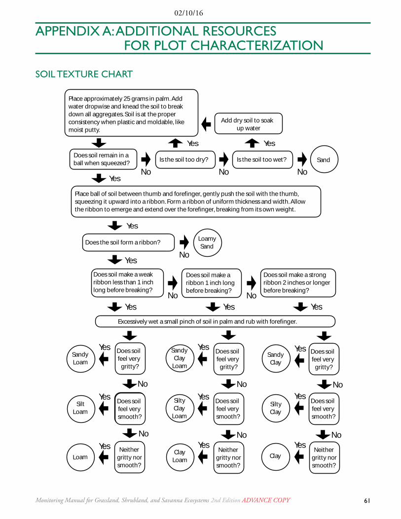
02/10/16
61Monitoring Manual for Grassland, Shrubland, and Savanna Ecosystems 2nd Edition AdvAncE copy
APPENDIx A: ADDITIONAL RESOURCES FOR PLOT CHARACTERIZATION
SOIL TExTURE CHART
Place approximately 25 grams in palm. Add water dropwise and knead the soil to break down all aggregates. Soil is at the proper consistency when plastic and moldable, likemoist putty.
Does soil remain in a ball when squeezed? Is the soil too dry? Is the soil too wet? Sand
Place ball of soil between thumb and forefinger, gently push the soil with the thumb,squeezing it upward into a ribbon. Form a ribbon of uniform thickness and width. Allowthe ribbon to emerge and extend over the forefinger, breaking from its own weight.
Does the soil form a ribbon? LoamySand
Does soil make a weakribbon less than 1 inch long before breaking?
Does soil make a ribbon 1 inch long before breaking?
Does soil make a strong ribbon 2 inches or longer before breaking?
Excessively wet a small pinch of soil in palm and rub with forefinger.
SandyLoam
SiltLoam
Loam
SandyClayLoam
SiltyClayLoam
ClayLoam
SandyClay
SiltyClay
Clay
Does soil feel verygritty?
Neithergritty nor smooth?
Does soil feel verygritty?
Does soil feel verysmooth?
Neithergritty nor smooth?
Does soil feel verygritty?
Does soil feel verysmooth?
Neithergritty nor smooth?
Yes
Yes
Yes
YesNo
No
Does soil feel verysmooth?
Yes
Yes
Yes Yes
Yes
Yes
Yes
Yes
No
Yes
No
Add dry soil to soakup water
No
No
Yes YesNoNo
No
No No No
YesYes
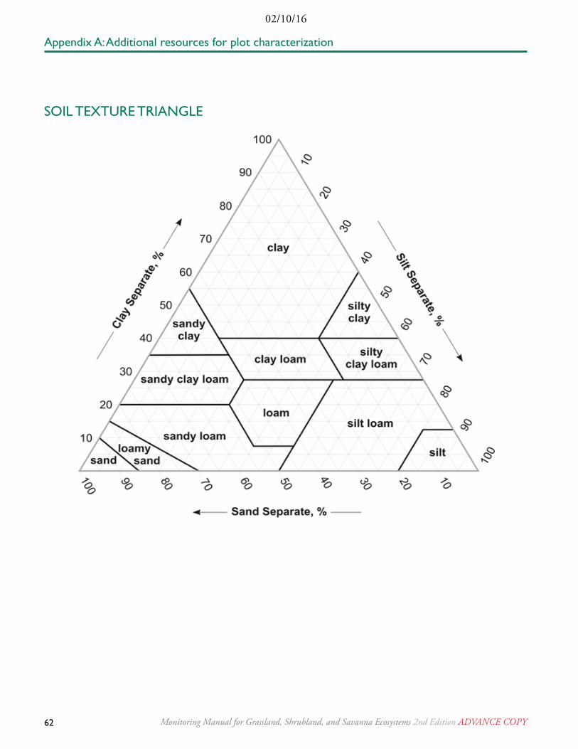
62 Monitoring Manual for Grassland, Shrubland, and Savanna Ecosystems 2nd Edition AdvAncE copy
02/10/16
Appendix A: Additional resources for plot characterization
SOIL TExTURE TRIANGLE

02/10/16
63Monitoring Manual for Grassland, Shrubland, and Savanna Ecosystems 2nd Edition AdvAncE copy
APPENDIx B: DATA SHEETS
The data sheets which accompany the methods described in this Core Methods volume are:• Equipment Checklist • Plot Checklist• Unknown Plant Record • QA and QC • Plot Characterization• Plot Observation• Photo points• Line-point intercept• Line-point intercept with height• Vegetation height• Gap intercept• Soil stability• Species inventory
Electronic data forms and the Database for Inventory, Monitoring, and Assessment (DIMA) are available at http://jornada.nmsu.edu/monit-assess.
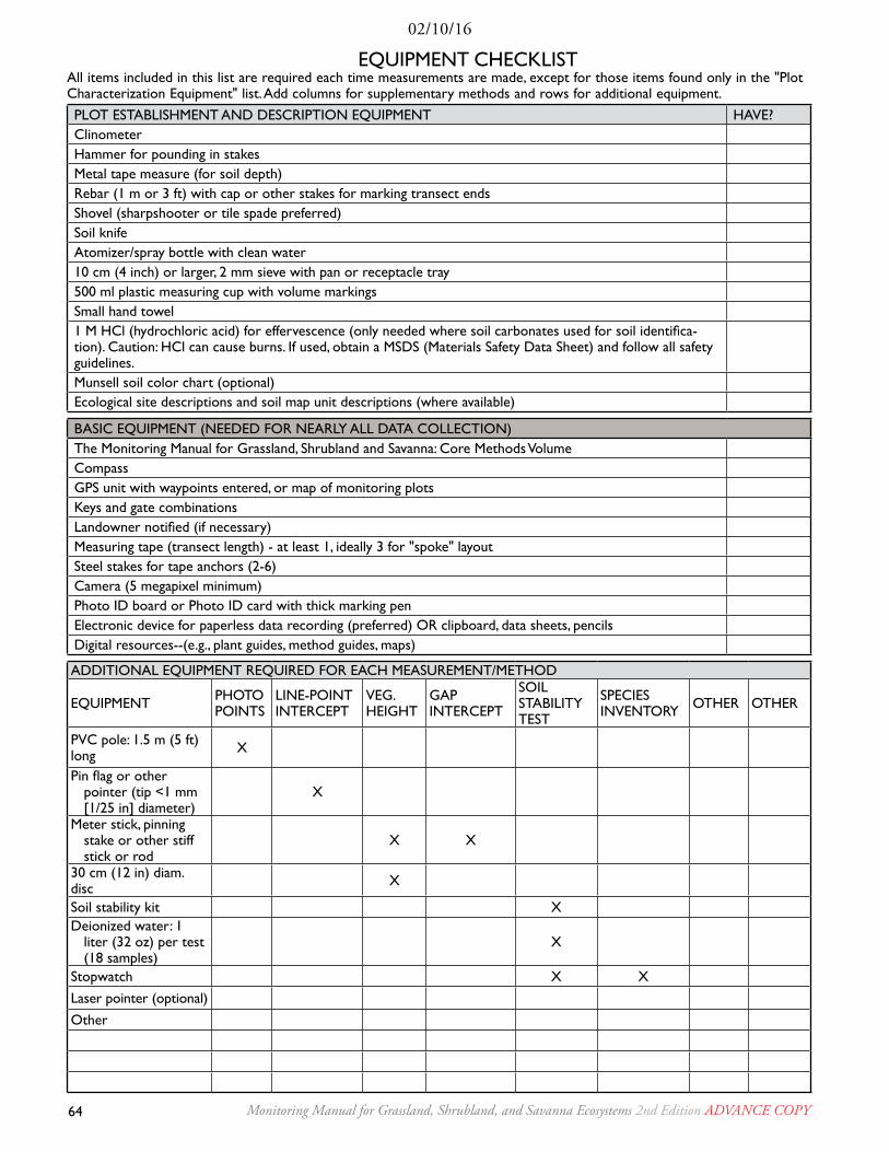
64 Monitoring Manual for Grassland, Shrubland, and Savanna Ecosystems 2nd Edition AdvAncE copy
02/10/16
EQUIPMENT CHECKLIST All items included in this list are required each time measurements are made, except for those items found only in the "Plot Characterization Equipment" list. Add columns for supplementary methods and rows for additional equipment. PLOT ESTABLISHMENT AND DESCRIPTION EQUIPMENT HAVE?ClinometerHammer for pounding in stakesMetal tape measure (for soil depth)Rebar (1 m or 3 ft) with cap or other stakes for marking transect endsShovel (sharpshooter or tile spade preferred)Soil knifeAtomizer/spray bottle with clean water10 cm (4 inch) or larger, 2 mm sieve with pan or receptacle tray500 ml plastic measuring cup with volume markingsSmall hand towel1 M HCl (hydrochloric acid) for effervescence (only needed where soil carbonates used for soil identifica-tion). Caution: HCl can cause burns. If used, obtain a MSDS (Materials Safety Data Sheet) and follow all safety guidelines.Munsell soil color chart (optional)Ecological site descriptions and soil map unit descriptions (where available)
BASIC EQUIPMENT (NEEDED FOR NEARLy ALL DATA COLLECTION)The Monitoring Manual for Grassland, Shrubland and Savanna: Core Methods Volume CompassGPS unit with waypoints entered, or map of monitoring plotsKeys and gate combinationsLandowner notified (if necessary)Measuring tape (transect length) - at least 1, ideally 3 for "spoke" layoutSteel stakes for tape anchors (2-6)Camera (5 megapixel minimum)Photo ID board or Photo ID card with thick marking penElectronic device for paperless data recording (preferred) OR clipboard, data sheets, pencilsDigital resources--(e.g., plant guides, method guides, maps)
ADDITIONAL EQUIPMENT REQUIRED FOR EACH MEASUREMENT/METHOD
EQUIPMENT PHOTO POINTS
LINE-POINT INTERCEPT
VEG.HEIGHT
GAP INTERCEPT
SOIL STABILITy TEST
SPECIES INVENTORy OTHER OTHER
PVC pole: 1.5 m (5 ft) long x
Pin flag or other pointer (tip <1 mm [1/25 in] diameter)
x
Meter stick, pinning stake or other stiff stick or rod
x x
30 cm (12 in) diam. disc x
Soil stability kit xDeionized water: 1
liter (32 oz) per test (18 samples)
x
Stopwatch x xLaser pointer (optional)Other

02/10/16
65Monitoring Manual for Grassland, Shrubland, and Savanna Ecosystems 2nd Edition AdvAncE copy
PLOT CHECKLISTTo be completed at each plot after methods are complete
☐ Plot Characterization ☐ Plot Observation ☐ Photo points
# of photos ______ ☐ Line-point intercept
Transect % bare ground % total foliar cover % between plant ground cover
☐ Vegetation heightTransect Woody Ht. Min Woody Ht. Max Herbaceous Ht. Min Herbaceous Ht. Max
☐ Gap interceptTransect % 25-50 cm % 51-100 cm % 101-200 cm % >200 cm
☐ Soil stabilityAll samples Avg. Protect Surface Avg. Unprotected Surface Avg.
☐ Species inventory# of species ______
Comments

66 Monitoring Manual for Grassland, Shrubland, and Savanna Ecosystems 2nd Edition AdvAncE copy
02/10/16
Proj
ect:
Fiel
d Se
ason
: C
olle
ctor
(s):
Page
___
_ of
___
_
Unk
now
n Pl
ant
IDPl
ant
Cod
eSc
ient
ific
Nam
eFa
mily
Com
mon
Nam
ePl
ot ID
Not
es
UN
KN
OW
N P
LAN
T T
RA
CK
ING
SH
EET
Dat
a en
try
Dat
e
E
rror
che
ck
D
ate

02/10/16
67Monitoring Manual for Grassland, Shrubland, and Savanna Ecosystems 2nd Edition AdvAncE copy
QUALITy ASSURANCE AND QUALITy CONTROL DATA SHEET
Plot: Date Monitored:Methods Performed:
Peop
le
Data Manager(s):
Data Recorder(s)/Observer(s):
Data Entry: Error Check:
Name: Calibration Date:
QA and QC Notes:

68 Monitoring Manual for Grassland, Shrubland, and Savanna Ecosystems 2nd Edition AdvAncE copy
02/10/16
Site: Ownership: Establishment Date:
Plot ID: Visit Date:
Observer(s):
GPS Coordinate System: Datum : Zone (if applicable): Elevation ☐m ☐ft
Latitude Longitude
Plot Center
Transect Azimuth Length☐m ☐ft
Transect Start Slope (%)Latitude* Longitude
Aspect
Directions to the plot (or location where GPS track log is stored):
Draw the plot (include transect locations relative to plot center, soil pit location, roads, power lines, etc.). Draw on back of sheet if needed:
Landscape Unit/Position☐ Hill/Mountain1
☐ Summit2 ☐ Shoulder3 ☐ Backslope4
☐ Alluvial Fan5
☐ Terrace6
☐ Tread7 ☐ Riser8
☐ Floodplain/Basin9 ☐ Flat/Plain10 ☐ Playa11
☐ Dunes12
☐ Other -
Soil Horizon
Depth** ☐cm ☐in
Rock fragment type & vol (%)Texture % Clay Eff.
Color☐dry
☐moistStructure NotesGravel
2-76 mmCobbles
76-250 mmStones
250-600 mm
-
-
-
-
-
-
-
Map Unit Component: Ecological Site:
* Grey text indicates that the information is recommended but not required. Data availability and observer qualifications will determine if the boxes in grey are completed.
* *If soil horizon identification is not possible, use the following standard depths: 0-1 cm (0-0.5 in), 1-10 cm (0.5-4 in), 10-20 cm (4-8 in), 20-50 cm (8-20 in), 50-70 cm (20-28 in).
PLOT CHARACTERIZATION DATA SHEETComplete when plot is established
1 5 6 9 10 11 12
2 3
47
8
Vertical (Down) Slope Shape
☐ Convex ☐ Concave ☐ Linear \Horizontal (Across) Slope Shape
☐ Convex ☐ Concave ☐ Linear
) )
\
Data entry Date Error check Date Page of
))

02/10/16
69Monitoring Manual for Grassland, Shrubland, and Savanna Ecosystems 2nd Edition AdvAncE copy
Complete each time data are recorded at each plot
Describe management history (e.g., grazing plan, prescribed fire, shrub control, seeding, plowing, water units):
Describe wildlife use (e.g., type, species identified, and condition):
Describe livestock use (e.g., species, evidence, and intensity):
Describe off-site influences (e.g., transmission lines, mines, roads):
Additional visible disturbances and remarks (e.g., invasive species, evidence of fire, pests and pathogens):
Recent WeatherPrecip.
☐cm ☐in Data SourcePast 12 Months☐ Drought ☐ Normal ☐ Wet
Past 13 - 24 Months☐ Drought ☐ Normal ☐ Wet
Signs of Erosion Class 5 Class 4 Class 3 Class 2 Class 1
Rills ☐ Widespread (>10) AND long (>2')
☐ Common (>5) AND long (>2')
☐ Common (>5) OR long (>2')
☐ Very few (<5) AND short (<2`) ☐ None
Gullies ☐ Active headcut, unstable sides
☐ Active headcut, par-tially stable sides
☐ Active headcut, stable sides
☐ Inactive. Stable throughout ☐ None
Pedestals☐ Widespread throughout
area. Common exposed roots
☐ Common in flow paths. Occasional exposed roots.
☐ Common in flow paths. Roots rarely exposed
☐ Few in flow paths and interspaces only. No exposed roots
☐ None
Deposition/Runoff ☐ Dominates the plot. ☐ Widespread ☐ Common ☐ Rare ☐ None
Water Flow Patterns
☐ Very long (50'); numerous; unstable with active erosion; almost always connected
☐ Long (20-50'), very common, and usually connected
☐ Moderately long (5-20'), rare, common, and often connected
☐ Very short (<5'), rare, and occasionally connected
☐ None
Sheet Erosion ☐ Dominates the plot ☐ Widespread ☐ Common ☐ Rare ☐ None
Other: ☐ Dominates the plot ☐ Widespread ☐ Common ☐ Rare ☐ None
Observer(s): Visit Date:
Data collection methods, citations, and modifications:
Plot Photos
Photo # Description
PLOT OBSERVATION DATA SHEET
Data entry Date Error check Date Page of
70 Monitoring Manual for Grassland, Shrubland, and Savanna Ecosystems 2nd Edition AdvAncE copy
02/10/16
Site:
Date:
Plot:
Line #:
Direction:
Photo ID Card

02/10/16
71Monitoring Manual for Grassland, Shrubland, and Savanna Ecosystems 2nd Edition AdvAncE copy
PT. TOP LAyER
LOWER LAyERS SOIL SURFACE PT. TOP
LAyERLOWER LAyERS SOIL
SURFACECODE 1 CODE 2 CODE 3 CODE 1 CODE 2 CODE 3
1 26
2 27
3 28
4 29
5 30
6 31
7 32
8 33
9 34
10 35
11 36
12 37
13 38
14 39
15 40
16 41
17 42
18 43
19 44
20 45
21 46
22 47
23 48
24 49
25 50
LINE-POINT INTERCEPT DATA SHEET
% foliar cover = top layer pts (1st col) x 2 = %% bare ground* = pts (w/N over S) x 2 = %% basal cover = plant base pts (last col) x 2 = %
Top layer codes: Species code, common name, or N (no cover).Lower layers codes: Species code, common name, HL (herbaceous litter), WL (woody litter, > 5 mm (~1/4 in) diameter), NL (non-vegetative litter), VL (vagrant lichen).
* For NRI, bare ground occurs ONLy when Top layer = N, Lower layers are empty (no litter), and Soil surface = S or Cy.
Shaded cells for calculations
UNKNOWN SPECIES CODES:AF#=annual forbPF#=perennial forb
AG#=annual graminoidPG#=perennial graminoidSH#=shrubTR#=tree
SOIL SURFACE (DO NOT USE LITTER):
R=Rock** (≥ 5 mm or ~1/4 in diameter)
BR=BedrockD=DuffM=Moss
LC=Visible lichen on soil S=Soil
Data entry Date Error check Date
** Optional: use rock fragment classes in place of "R": GR (5-76 mm), CB (76-250 mm), ST (250 mm-600 mm), By (>600 mm)
Page ofPlot: Line: Observer: Recorder:
Azimuth: Date: Intercept (Point) Spacing Interval: ☐ cm ☐ in

72 Monitoring Manual for Grassland, Shrubland, and Savanna Ecosystems 2nd Edition AdvAncE copy
02/10/16
PT. TOP LAyERLOWER LAyERS SOIL
SURFACEWOODy SPECIES
WOODy HEIGHT
HERB. SPECIES
HERB. HEIGHTCODE 1 CODE 2 CODE 3
1
2
3
4
5
6
7
8
9
10
11
12
13
14
15
16
17
18
19
20
21
22
23
24
25
LINE-POINT INTERCEPT WITH HEIGHT DATA SHEETShaded cells for calculations
% foliar cover = top layer pts (1st col) x 4 = %% bare ground* = pts (w/N over S) x 4 = %% basal cover = plant base pts (last col) x 4 = %
Top layer codes: Species code, common name, or N (no cover).Lower layers codes: Species code, common name, HL (herbaceous litter), WL (woody litter, > 5 mm (~1/4 in) diameter), NL (non-vegetative litter), VL (vagrant lichen).
* For NRI, bare ground occurs ONLy when Top layer = N, Lower layers are empty (no litter), and Soil surface = S or Cy.
UNKNOWN SPECIES CODES:AF#=annual forbPF#=perennial forb
AG#=annual graminoidPG#=perennial graminoidSH#=shrubTR#=tree
SOIL SURFACE (DO NOT USE LITTER):
R=Rock** (≥ 5 mm or ~1/4 in diameter)
BR=BedrockD=DuffM=Moss
LC=Visible lichen on soil S=Soil
Data entry Date Error check Date
** Optional: use rock fragment classes in place of "R": GR (5-76 mm), CB (76-250 mm), ST (250 mm-600 mm), By (>600 mm)
Page of
Plot: Line: Observer: Recorder:
Azimuth: Date: Intercept (Point) Spacing Interval: ☐ cm ☐ in Height: ☐ cm ☐in

02/10/16
73Monitoring Manual for Grassland, Shrubland, and Savanna Ecosystems 2nd Edition AdvAncE copy
Data entry Date Error check Date
VEGETATION HEIGHT DATA SHEET
POINT SPECIES WOODy HT SPECIES HERBACEOUS HT
Average vegetation height = ____________________ Average woody height = __________________________
Average herbaceous height = ___________________
Page of
Plot: Line: Observer: Recorder:
Azimuth: Date: Intercept (Point) Spacing Interval: ☐cm ☐in Height: ☐cm ☐in

74 Monitoring Manual for Grassland, Shrubland, and Savanna Ecosystems 2nd Edition AdvAncE copy
02/10/16
Circle one: includes only perennial vegetation OR includes annual and perennial vegetation
Canopy gaps: Minimum size = _____ ☐cm ☐ft Basal gaps: Minimum size = _____ ☐cm ☐ft
Start(cm/ft)
End(cm/ft)
Gap (cm) 25-50 51-100 101-200 > 200 Start(cm/ft)
End(cm/ft)
Gap (cm) 25-50 51-100 101-200 > 200size (ft) 1-2 2.1-3 3.1-6 > 6 size (ft) 1-2 2.1-3 3.1-6 > 6
SUM (cm/ft) SUM (cm/ft)
LINE LENGTH (cm/ft) LINE LENGTH (cm/ft)
SUM ÷ LINE LENGTH SUM ÷ LINE LENGTH
x 100 x 100 x 100 x 100 x 100 x 100 x 100 x 100
% of line in gaps % of line in gaps
Example: If SUM 25-50 = 1,573, Line Length = 5,000 cm, then % of line in gaps 25-50 cm = 100 x (SUM 25-50/line length) = 100 x (1,573/5,000) = 31.5%.
GAP INTERCEPT DATA SHEETShaded cells for calculations
Data entry Date Error check Date
Plot: Line: Observer: Recorder:
Azimuth: Date: Line length: ☐m ☐ ft Page of

02/10/16
75Monitoring Manual for Grassland, Shrubland, and Savanna Ecosystems 2nd Edition AdvAncE copy
Shad
ed c
ells
for
calc
ulat
ions
Dat
a en
try
D
ate
E
rror
che
ck
Dat
e
SOIL
STA
BILI
Ty
TES
T D
ATA
SH
EET
Veg
= N
C (
no p
eren
nial
can
opy)
; C (
pere
nnia
l cov
er)
OR
G (
gras
s or
gra
ss/s
hrub
mix
), F
(forb
), Sh
(sh
rub)
, T (
tree
); M
(ro
ot m
at)
# =
Stab
ility
val
ue (
1-6)
. Circ
le v
alue
if s
ampl
es a
re h
ydro
phob
ic.
Surf
ace
Line
___
In time
Dip
tim
eC
lass
Line
___
In time
Dip
tim
eC
lass
Line
___
In t
ime
Dip
tim
eC
lass
Line
___
In t
ime
Dip
tim
eC
lass
Line
___
In time
Dip
tim
eC
lass
Line
___
In time
Dip
tim
eC
lass
Pos
Veg
Pos
Veg
Pos
Veg
Pos
Veg
Pos
Veg
Pos
Veg
0:00
5:00
0:45
5:45
1:30
6:30
2:15
7:15
3:00
8:00
3:45
8:45
0:15
5:15
1:00
6:00
1:45
6:45
2:30
7:30
3:15
8:15
4:00
9:00
0:30
5:30
1:15
6:15
2:00
7:00
2:45
7:45
3:30
8:30
4:15
9:15
Not
es:
Subs
urfa
ce
Line
___
In time
Dip
tim
eC
lass
Line
___
In time
Dip
tim
eC
lass
Line
___
In t
ime
Dip
tim
eC
lass
Line
___
In t
ime
Dip
tim
eC
lass
Line
___
In time
Dip
tim
eC
lass
Line
___
In time
Dip
tim
eC
lass
Pos
Veg
Pos
Veg
Pos
Veg
Pos
Veg
Pos
Veg
Pos
Veg
0:00
5:00
0:45
5:45
1:30
6:30
2:15
7:15
3:00
8:00
3:45
8:45
0:15
5:15
1:00
6:00
1:45
6:45
2:30
7:30
3:15
8:15
4:00
9:00
0:30
5:30
1:15
6:15
2:00
7:00
2:45
7:45
3:30
8:30
4:15
9:15
Not
es:
Ave
rage
Soi
l Sta
bilit
y =
Sum
of R
anki
ngs
(i.e.
, #)
/ Tot
al N
umbe
r of
Sam
ples
Tak
en
Line
All
sam
ples
Prot
ecte
d sa
mpl
es(S
ampl
es w
ith V
eg =
C, M
, or
G, F
, Sh,
T, M
)U
npro
tect
ed s
ampl
es(S
ampl
es w
ith V
eg =
NC
)Su
rfac
eSu
bsur
face
Surf
ace
Subs
urfa
ceSu
rfac
eSu
bsur
face
Plot
Avg
.
Plot
Obs
erve
r
R
ecor
der
Dat
e
Page
of

76 Monitoring Manual for Grassland, Shrubland, and Savanna Ecosystems 2nd Edition AdvAncE copy
02/10/16
NO. SPECIES FUNCTIONAL GROUP NOTES
1
2
3
4
5
6
7
8
9
10
11
12
13
14
15
16
17
18
19
20
21
22
23
24
25
26
27
28
29
30
SPECIES INVENTORy DATA SHEET
Total number of species: Non-natives spp. Rare species
# Tree spp. # Shrub spp. # Grass spp. # Forb spp.
# Perennial spp. ________
# Annual/Biennial spp. ________
Page of Search Time: Plot: Observer: Recorder:
Date: Plot Shape: Inventory Area: ☐ m2 ☐ ft2
Data entry Date Error check Date
Notes (e.g., 15 minute search captured 75% of species diversity)

02/10/16
77Monitoring Manual for Grassland, Shrubland, and Savanna Ecosystems 2nd Edition AdvAncE copy
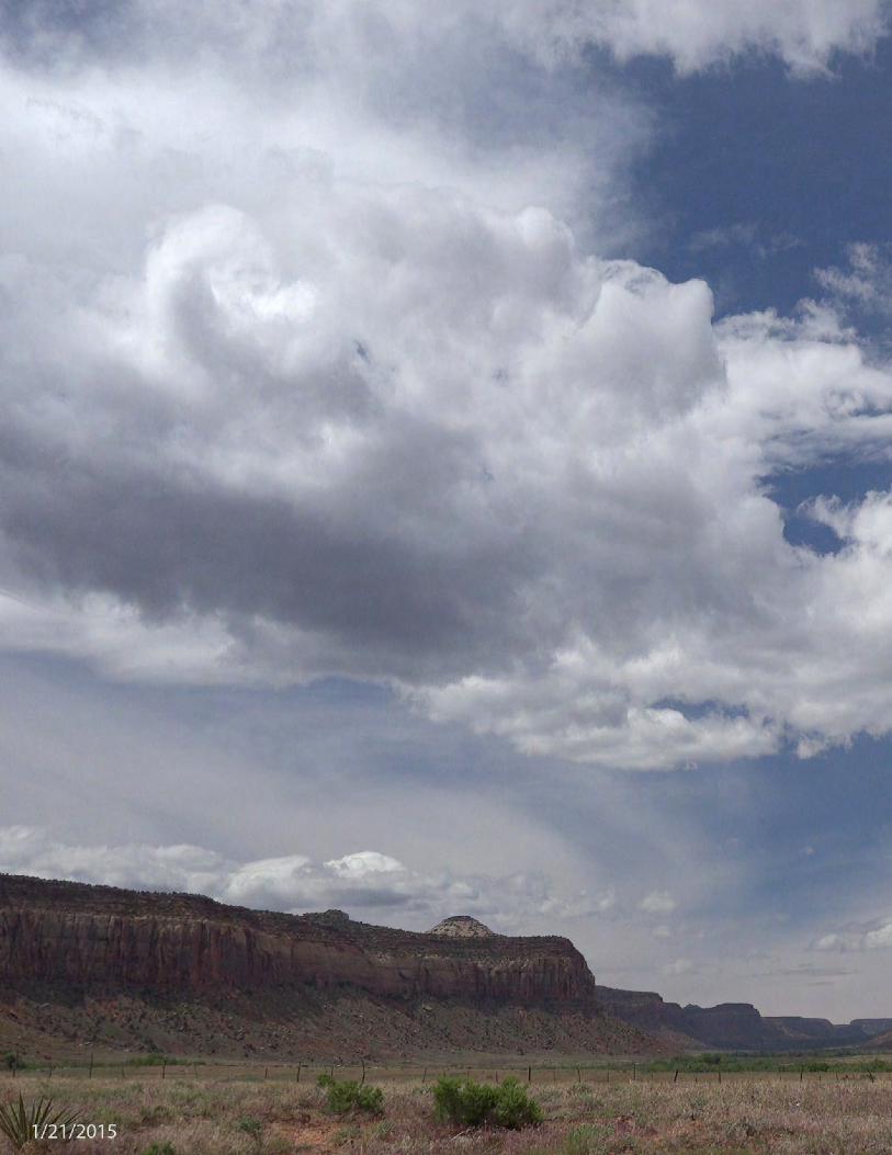
78 Monitoring Manual for Grassland, Shrubland, and Savanna Ecosystems 2nd Edition AdvAncE copy
02/10/16


