Monitoring of forty years of agricultural expansion in the ...

Article

Monitoring of forty years of agricultural expansion in the Oum

Er Rbia valley (Morocco). The use of Google Earth Engine com-

pared to Sentinel Application Platform

María Adell 1, José Antonio Domínguez-Gómez 2 and Juan Soria 1,*

1 Cavanilles Institute of Biodiversity and Evolutive Biology. University of Valencia. 46980 – Paterna (Spain);

[email protected]; [email protected] 2 IMIDA - GIS and Remote Sensing, Murcia Institute of Agri-Food Research and Development, C/Mayor s/n,

La Alberca, 30150 Murcia, Spain; [email protected]

* Correspondence: [email protected]

Abstract: Agriculture in Morocco has been extensive until the middle of the 20th century due to the

distribution of rainfall and the availability of water. In the middle of the last century hydraulic

works were built that allowed the transition to intensive agriculture by the increase of irrigated

areas, allowing that in the territories where there is water for irrigation and the climate allows it, the

crops adapt to the demands of the market. The objective of the study is to assess by satellite images

the land cover between 1985 and 2020, analyzing the changes in cultivation areas, as well as the

changes in desert, sub-desert and forest areas of the Oum Er Rbia hydrological basin in Morocco.

Landsat satellite images have been used since 1984 by the US government (Aerospace and Geolog-

ical Agencies). A series of vegetation indices (NDVI, RVI, TNDVI and EVI) have been used; among

which TNDVI (Transformed Normalized Vegetation Index) stands out for its better accuracy, which

has allowed us to distinguish vegetation in cultivated and forest areas, as well as arid zones. In

addition, the study has compared the use of two methodologies to calculate changes in the coverage

of the Earth’s surface, has used local image processing from the Sentinel Application Platform tool

and has also used the Google Earth Engine tool. The latter being the most optimal, although at the

moment it has great limitations. In both methodologies and in the different indices it has been pos-

sible to observe during these 35 years as the cultivated area has increased (related to the availability

of water by the construction of reservoirs and canals), how plant cover has improved in forest areas,

and a range of variations in arid areas.

Keywords: African agriculture; Irrigation; Landsat; Remote Sensing; Reservoir.

1. Introduction

Rainfed and irrigated agriculture in North Africa in general has been characterized

by human presence throughout history. The low population density has shaped an agrar-

ian or agricultural-livestock system, especially in modern and contemporary times. Agri-

culture has been extensive until the 20th century, when hydraulic works were carried out

that allowed the irrigation of many areas and the transition from extensive agriculture to

intensive agriculture [1]. The tribal organization of the population in the mountainous and

sub-desert territory also contributed to the existence of collectivities that carried out agri-

cultural and livestock development in local communities [2].

Water is an essential resource and in Morocco the management of this resource is

even more vital, especially due to its semi-arid climate and limited water availability, in

addition to the effects of climate change that are already being felt, since in the last three

decades the country has suffered five periods of severe drought, exacerbating the prob-

lems of the region [3]. It is a country of contrasts between mountain ranges that are diffi-

cult to access and vast plains open to the Atlantic; between a relatively humid ocean front

and large desert expanses to the east and south. The presence of the Atlas Mountains

Preprints (www.preprints.org) | NOT PEER-REVIEWED | Posted: 1 November 2021

© 2021 by the author(s). Distributed under a Creative Commons CC BY license.

mailto:[email protected]

http://creativecommons.org/licenses/by/4.0/

conditions the climatic variability of Northern Morocco. The territories located to the NW

of it, open to the Atlantic, are characterized by a more humid climate, while those located

to the SE, facing the Sahara, account for 60% of the national territory, have an arid climate

and rainfall is less than 400 mm per year. The distribution of rainfall and the availability

of water for irrigation determine agricultural use.

Because of its climatic characterization, the state considers agriculture as territorial-

ized, indicating that there are regions where this activity is not possible and others where

it is a major economic asset [4]. The territory of Morocco is divided into 16 regions, which

in turn are divided into provinces and communes. In each province there is a ministerial

delegation that manages the administrative aspects of agricultural activity. The next level

of organization downwards are the Agricultural Valorization Offices, which are located

in each of the areas with large irrigated territories and their nearby rainfed areas. In semi-

arid regions, with rainfall of less than 400 mm per year, agricultural development is car-

ried out at the highest altitudes, to take advantage of the mild climate, while in areas with

rainfall of more than 400 mm, the agricultural strategy aims at intensification. In areas

where irrigation water is available, crops are adapted to market demands. In mountain

areas, they are dedicated to pasture and forest use, with priority given to environmental

conservation. Finally, in desert and oasis areas, the uses are unique and very site-specific

[4].

In 1966, the U.S. Geological Survey proposed the creation of Earth Resources Obser-

vation Satellites, but it was not until 1972 that the first satellite, called Earth Resources

Technology Satellite (ERTS-1), was in orbit. Later, in 1975, it was renamed Landsat at the

time of the launch of the Landsat-2 satellite. From that time to the present, the Landsat

mission had continuity, with Landsat-9 currently in its manufacturing [5]. This has pro-

vided a database of images of the planet unimaginable in its beginnings, whose continuity

over time allows the elaboration of time series studies such as the one presented here.

The information obtained by the satellite from the air is related to the reflectivity that

the planet emits in the upper atmosphere, known as TOA. The information is collected in

different bands whose characteristics initially covered the visible spectrum in the three

primary colors of light (blue, green and red) known as the RGB triad and in the near in-

frared (NIR). With the improvement of sensors in both quality and definition, the meas-

urement bands have increased, as has the size of the measurement pixel, which is getting

smaller and smaller and with greater spatial definition.

The treatment of the different bands could be done according to the researcher's cri-

teria, producing the initial works about vegetation [6-8] and a few years later about water

bodies [9,10]. When a sufficient database existed, different treatments of the bands were

created to be used for the simplest uses, such as studies of the presence of water bodies,

vegetation studies and studies on the earth's crust and its different coverages (ice, dry

land, vegetation, water, urban areas, temperature, etc.), such as those of Dowdeswell et

al. [11] on the distribution of ice masses using Landsat and SPOT images; the work of Toll

[12] on land use using Landsat or that of Otterman and Tucker [13] on the relationship

between temperature, albedo and vegetation also using Landsat images.

In our case, we have explored the possibilities of the already established vegetation

indices to describe the variations of agricultural areas, considering the time period, the

territory under study and the computer tools to process the available information. The

need to compare Landsat-5 and Landsat-8 images has considered using indexes based on

the satellite's green, red and infrared bands. On the other hand, the information available

in Google Earth Engine at the time of the study (summer 2021) has also been used to com-

pare the results obtained with this new system with those obtained by local processing of

satellite images downloaded from existing distribution servers.

The most used current vegetation indices are known by the abbreviation of their

name indicating the procedure used to calculate them. The following list presents those

that use Landsat visible and infrared bands for calculation:

Normalized Difference Vegetation Index NDVI [14]


Ratio Vegetation Index RVI [15]

Transformed Normalized Difference Vegetation Index TNDVI [16]

Soil Adjusted Vegetation Index SAVI [17]

Difference Vegetation Index DVI [18]

Enhanced Vegetation Index EVI [19]

Our hypothesis and objectives were that that the increase of the agricultural area in

certain provinces of Morocco has been due to the availability of regulated water and the

construction of hydraulic works for its conduction to areas to increase agricultural pro-

duction. For this purpose, the Oum Er Rbia river valley has been considered as a case

study, evaluating by means of several vegetation indices applied to satellite images, how

the agricultural area has been changing from the 1980s to the present. The contribution of

this study lies in comparing for the first time the use of the Google Earth Engine tool with

local processing by SNAP and whether there are differences in terms of the results ob-

tained, presenting the advantages and disadvantages of each system.

2. Materials and Methods

2.1 Study site

The Oum Er-Rbia river is located in Morocco (Figure 1), in the north of the African

continent. It is one of the most important rivers in the country, its source is located in the

Middle Atlas Mountains, 40 km from Khenifra (1800 m a.s.l.), in the province of Meknès

Tafilalet, the middle section runs through the province of Tadla Azilal and the riverbed is

the geographical boundary of the Grand Casablanca region to the north on the right bank

and Doukkala Abda to the south on the left bank. After approximately 550 km, it flows

into the Atlantic Ocean in the town of Azemmour, in the province of Doukkala Abda.

Figure 1. Location map of the Oum Er Rbia river in the provinces of Central Morocco (own elabo-

ration).

The hydrographic network is formed by the Oum Er Rbia river and its main tributar-

ies which are the Tassaout, El Abid and Lakhdar rivers on the left bank, which constitutes

the foothills of the Atlas Mountains. The right bank, on the other hand, is part of the so-

called "phosphate plateau" or Ouardigha Plateau, and is only drained by temporary


rivers. The amount of annual rainfall, which varies from 300 mm to 1100 mm and the

melting of snow from the Atlas Mountains, mean that the average supply at the mouth of

the river is considerable and regular and is estimated at 3680 hm3/year, with a minimum

of 1300 hm3 and a maximum of 8300 hm3 [20-23].

Fifteen reservoirs are currently built on the river, but the three main dams from head-

waters to mouth are Bin El Ouidane, Ahmed El Hansali and Al Massira, which are in-

tended to produce hydropower and supply water for urban use and supply to irrigated

agriculture, which is the main consumer of water in the river basin [24].

The study area corresponds to the Oum Er-Rbia river basin (Figure 2), which covers

an area of approximately 38,000 km2. With such a large surface area, there is great internal

variability, as the basin ranges from the Atlantic coast to the High Atlas (4,000 m a.s.l.).

The relief are intracontinental folded belts, which form the Atlas Mountains, shortened

with areas of plateaus that are poorly deformed tabular domains, generated by the clear

dominance of the Alpine orogeny [25]. The climate of the basin is Mediterranean with

cold, wet winters and hot, dry summers. Temperature varies between 10 ˚C and 50 ˚C

with mean minimum values of 3.5 °C in January and mean maximum values of 38 °C

August. Evaporation can reach 1600 to 1800 mm/year. The annual cycle in the entire basin

has a clear variation, it is divided into two periods, a wet one (from November to April)

and a dry one (from June to September, with July being the driest month), with the months

of May and October being transitory. There is a gradient in the basin ranging from arid to

semi-arid, with decreasing precipitation from east to west, due to the orographic effect of

the Atlas Mountains, with the average precipitation of the basin being 500 mm [20,21,26].

Figure 2. Map of the digital model of the basin, the fluvial layout and location of existing res-

ervoirs by their abbreviation, according to Table 1 (own elaboration).

The hydrographic network is formed by the Oum Er Rbia river and its main tributar-

ies which are the Tassaout, El Abid and Lakhdar on the left bank, which constitutes the

foothills of the Atlas Mountains. The right bank, on the other hand, is part of the so-called

"phosphate plateau" or Ouardigha Plateau, and is only drained by temporary rivers. The

amount of annual rainfall, which varies from 300 mm to 1100 mm and the melting of snow

from the Atlas Mountains, mean that the average supply at the mouth of the river is


considerable and regular and is estimated at 3680 hm3/year, with a minimum of 1300 hm3

and a maximum of 8300 hm3 [20-23].

The middle zone of the basin are plains formed by sedimentary rocks under a Qua-

ternary cover. It is an area between the Settat plateau to the south of marl-limestone for-

mation and the Berrechid plain to the north of sandstone-limestone with silt and clay soils.

The area is of high Plio-Quaternary tectonic activity due to the existence of major faults

[28]. The climate of the region is represented by Beni Mellal, at 500 m a.s.l. at the foot of

the mountain. The city has a mild climate with an average temperature of 17.3 ˚C, accord-

ing to the Köppen classification it is a subtropical Mediterranean climate (Csa) (Figure 3).

Annually it precipitates on average 558 millimeters, rainfall occurs throughout the year,

except for the summer season in the northern hemisphere.

Figure 3. Climogram in three towns in the study area of the Oum Er Rbia river: Azilal, in the upper basin; Beni-Mellal in

the middle basin and El Jadida at the mouth of the Atlantic.

The upper Oum Er-Rbia basin is a mountainous area of sandstone-karstic character,

geologically in the domain of the Middle Atlas, with an altitude variability ranging be-

tween 1,000 and 4,000 m a.s.l., generated by the convergence of the Eurasian and African

plates in the Cenozoic (Alpine Orogeny). It presents a great diversity of relief forms, with

large closed depressions, ravines, alluvial terraces and forested mountains which also in-

clude the central Hercynian massif in sedimentary Khenifra with intense volcanic activity

due to this orogeny that generated granitic intrusions on this, and a high limestone plat-

eau, the Ajdir plateau [22,23,29,30]. The climate of the region can be symbolized by the

climate of Azilal at 1,356 m a.s.l., according to Köpen the city has a humid subtropical

climate (Cfa) (Figure 3). The average temperature is 14 ˚C, with cool winters and hot hu-

mid summers. Precipitation is spread throughout the year and rains an average of 700

millimeters. In the upper river basin, about 1,100 millimeters are precipitated annually,

where it snows on average about 20 days per year [24].

The construction of reservoirs in the river basin begins in the middle of the 20th cen-

tury with an initial plan for irrigation of one million hectares, which had its origin in the

proposals of the French Protectorate in 1936 [31]. The large reservoirs act as regulators

and the small reservoirs have the mission of distributing the water through the canals that

take it to the irrigable areas. Of the fifteen reservoirs, seven have a capacity greater than

10 hm3, whose location is shown in Figure 2 and their data are presented in Table 1.

Table 1. Reservoirs with a capacity greater than 10 hm3 in the Oum Er Rbia river basin, indicating

the year of commissioning and the planned extension of their irrigable area. For each one, its ab-

breviation in three letters is indicated, year of construction and planned irrigable area.

Reservoir Abrev. River Year Volume (hm3) Irrigable (ha)

Al Massira ALM Oum Rbia 1979 2,760 96,000

Imfout IMF Oum Rbia 1944 27

El Hansali ELH Oum Rbia 1997 740 36,000

Bin Ouidan BIN El Abid 1953 1,384 69,500


Ait Messaoud AIT Oum Rbia 2002 14

Moulay Youssef MOU Tassaout 1969 175

Hassan I HAS Lahkdar 1986 263 40,000

The largest reservoir is Al Massira and downstream is Imfout which is the closest to

the mouth (Figure 2) and distributes through the canals of the lower coastal area. Near the

headwaters is El Hansali and then Ait Messaoud which is the distributor in the middle

section in the irrigable area of Beni Amir on the right bank. On the El Abid tributary (on

the left) is Bin El Ouidan, the first large reservoir to be commissioned in Morocco, which

sends the water through a canal to the irrigable area of Beni Mellal. Of smaller size are the

Hassan I reservoir on the Lahkdar river (tributary on the left) and the Moulay Youssef

reservoir on the Tassaout river (tributary on the left of the Lahkdar).

2.2 Methodology

To make the location map of the region, free access layers of the continents, African

countries, cities and provinces of Morocco were searched, the layers were downloaded

from Natural Earth (https://www.naturalearthdata.com/). To build the location map (Fig-

ure 1), the ArcGIS tool was used. The base layer of the map is the countries of the world,

from which the country of Morocco was extracted to highlight the area. This process was

carried out from a selection by attributes of the country and exported as another layer, in

order to give it a different color from the rest of the countries. After this, the same was

done with the layer of provinces of Morocco, the profile of the basic Oum Er Rbia river

was placed, and the provinces through which the river passes were selected, after this the

provinces were exported and a layer was generated. To mark the most important cities

within the provinces, a clip was made, the layer of points of the most important cities of

Morocco was crossed with the layer of the provinces that was created previously. From

this process, a new layer of dots was generated, which constitutes the most important

cities of the provinces through which the Oum Er Rbia river flows. In this map, the river

profile corresponds to a discharge of a vector of lines representing the most important

rivers in the world. From this layer an extraction was performed to obtain in one layer

only the Oum Er Rbia river.

In addition to these, a Digital Elevation Model (DEM) was obtained to make the pro-

file of the basin and the Oum Er Rbia riverbed, with a resolution of 250 meters. To obtain

the basin, the first thing that was done was to perform the process called fill, which fills

the basin, i.e., the pixels of the DEM are not left without values. After this, a flow direction

is made, which estimates how a drop of water would move, in each pixel a direction is

drawn following the criterion of greater slope. After this, a point was created at the mouth

of the river to obtain the drainage basin. With the point and the flow direction layer, the

watershed profile of the Oum Er Rbia river drainage basin was created with the watershed

tool. With this process a map of the basin profile with the altitude of the basin was ob-

tained. To create the line representing the river on this map, a photointerpretation was

made with the ArcGIS base map.

To conduct the study in the region, once known exact location and the surface of the

basin, the Landsat images corresponding to each year were downloaded from the USGS

server. Five Landsat scenes are needed to complete the Oum Er Rbia basin area. The study

starts in the year 1985 with Landsat 4 images and ends in the year 2020 with Landsat 8

images. It was decided to be done in five-year intervals, so a total of 40 images from Land-

sat 4, Landsat 5 and Landsat 8 satellites were needed. The downloaded images with dates

can be seen in Table 2. All images were taken in the same season, between April and Sep-

tember.

When all the images were downloaded, they were processed with the SNAP tool

(Brockmann Consult Gmbh, Germany), with the mosaicking tool the five images that

make up the study area for each year were joined. Thus, there is one product for each year,

i.e. eight products, made up of five satellite scenes for each product.


After having all the products for each year, we proceeded to calculate the vegetation

indices. In this case, the three most common indices, known by their abbreviations NDVI,

TNDVI and RVI, were tested.

NDVI (Normalized Difference Vegetation Index) is a classic indicator of the green-

ness of biomes, and is useful for understanding vegetation density and assessing changes

in plant health. It is the most widely used index of vegetation globally, as it compensates

for changes in illumination, land surface slope among other things. NDVI is calculated as

a ratio between red (R) and near infrared (NIR) values [14]. Its formula is as follows:

Landsat 4-5: 𝑁𝐷𝑉𝐼 =𝐵𝑎𝑛𝑑 4−𝐵𝑎𝑛𝑑 3

𝐵𝑎𝑛𝑑 4+𝐵𝑎𝑛𝑑 3 (1)

Landsat 8: 𝑁𝐷𝑉𝐼 =𝐵𝑎𝑛𝑑 5−𝐵𝑎𝑛𝑑 4

𝐵𝑎𝑛𝑑 5+𝐵𝑎𝑛𝑑 4 (2)

This determines values between -1 and 1, with values closer to 1 being those with a

high density of vegetation and those closer to -1 being water, snow, and around 0 being

bare soil or rocks.

TNDVI (Transformed Normalized Difference Vegetation Index) is the transfor-

mation of NDVI so as not to work with negative values. TNDVI indicates a slightly better

correlation than the original one between the amount of green biomass found in a consid-

ered pixel [32]. Its formula is:

Landsat 4-5: 𝑇𝑁𝐷𝑉𝐼 = √(𝐵𝑎𝑛𝑑 4−𝐵𝑎𝑛𝑑 3

𝐵𝑎𝑛𝑑 4+𝐵𝑎𝑛𝑑 3) + 0.5 (3)

Landsat 8: 𝑇𝑁𝐷𝑉𝐼 = √(𝐵𝑎𝑛𝑑 5−𝐵𝑎𝑛𝑑 4

𝐵𝑎𝑛𝑑 5+𝐵𝑎𝑛𝑑 4) + 0.5 (4)

As a result, the lowest values are found in built-up areas and water bodies [32].

The RVI (Ratio Vegetation Index) is an index that highlights the contrast between

vegetation and soil, because it is sensitive to the optical properties of the soil, but not to

lighting conditions. It is mostly used to estimate leaf area biomass [33]. Its formula is as

follows:

Landsat 4-5: 𝑁𝐷𝑉𝐼 =𝐵𝑎𝑛𝑑 4

𝐵𝑎𝑛𝑑 3 (5)

Landsat 8: 𝑁𝐷𝑉𝐼 =𝐵𝑎𝑛𝑑 5

𝐵𝑎𝑛𝑑 4 (6)

When the values are high they reflect the presence of vegetation, and when they are

low they represent soil, water, etc. [33].

With respect to the Google Earth Engine (GEE) tool, it is accessed through a web

service (https://explorer.earthengine.google.com/#workspace) in which after registering

one can access various types of products already calculated from Landsat 5 images in the

period 1985-2010 and Landsat 8 in the period 2013-2020. One of the products is the vege-

tation index EVI, calculated according to the following formulas [19]:

Landsat 4-5: 𝐸𝑉𝐼 = 2,5 ∗(𝐵𝑎𝑛𝑑 4−𝐵𝑎𝑛𝑑 3)

(𝐵𝑎𝑛𝑑 4+6∗𝐵𝑎𝑛𝑑 3−7,5∗𝐵𝑎𝑛𝑑 1+1) (7)

Landsat 8: 𝐸𝑉𝐼 = 2,5 ∗(𝐵𝑎𝑛𝑑 5−𝐵𝑎𝑛𝑑 4)

(𝐵𝑎𝑛𝑑 5+6∗𝐵𝑎𝑛𝑑 4−7,5∗𝐵𝑎𝑛𝑑 2+1) (8)

After performing the calculation of each index for each annual product, 32 products

remain in total, i.e., four products from each year. Then the same intervals were adjusted

for each index, i.e. the products of each year of the same index have the same intervals to

be able to compare with each other.

To calculate how much vegetation is in the watershed we need to insert the vector

layer that was created that delimits the watershed. Once inserted in each product, we pro-

ceeded to create the histogram of the image using the vector layer, we calculate the num-

ber of pixels of each type that are in the watershed area. When the histogram was calcu-

lated, the data were extracted from which a table was created showing the number of

pixels that made up each interval. Thus it was possible to calculate the area in square

kilometers of each class, since the resolution of the image is known, which is 30 meters, so

each pixel corresponds to 900 square meters.


After having the results, the next step was to present the figures created from the

indexes. This presentation was made from ArcGIS, the SNAP figures were exported to

GeoTIFF format, so that they were georeferenced. They were opened in the ArcGIS tool

and the extract by mask tool was used, which extracts the data from the raster image that

we had exported through a vector layer, in this case the watershed profile.

For GEE products, the area of interest is exported in GeoTIFF format directly in the

web application interface, selecting the region of interest (ROI) in order to reduce the file

size and obtain the definition as a 30 x 30 m pixel Landsat. The file is then treated as those

obtained with SNAP.

3. Results

From the location of the study site, the Landsat satellite images needed to construct

the watershed were obtained. In total there are five for each year, corresponding to the

201-37, 201-38, 202-37, 202-38 and 203-37 strikes and passes. Table 2 shows the dates on

which the images were taken for each of these five in each year. The images were down-

loaded between 1985 and 2010 from the Landsat 4-5 TM satellite and those from 2015 and

2020 from Landsat 8 OLI.

Table 2. Dates of the satellite images used.

Path-Row 1985 1990 1995 2000 2005 2010 2015 2020

201-37 21/08/85 04/09/90 16/07/95 20/07/00 25/06/05 23/06/10 23/07/15 02/06/20 201-38 04/07/85 04/09/90 16/07/95 14/08/00 12/08/05 23/06/10 21/06/15 02/06/20 202-37 08/05/85 09/07/90 21/06/95 29/07/00 05/07/06 05/09/11 28/06/15 29/09/20

202-38 09/06/85 09/07/90 08/08/95 20/07/00 06/08/06 30/06/10 11/05/15 29/09/20

203-37 29/04/85 29/05/90 27/05/95 27/07/00 28/07/06 09/09/10 07/09/15 20/09/20

Figure 4 shows the result of joining the downloaded images after the mosaicking

process. The result shows the union and overlapping in some areas, as well as the irregu-

larities due to the composition of several images from different days.

Figure 5 is the cutout of Figure 3 with the basin profile created in false true color, i.e.

the Landsat 8 red, green and blue bands corresponding to band 4, band 3 and band 2,

respectively, have been applied. The colors of vegetation, water bodies, cities and the

phosphate mining area can be seen.

Figure 6 is the same as Figure 5 in which the bands have been combined to create a

false color. In this case the near infrared (NIR), red and green bands have been combined,

which in the case of the Landsat 8 satellite corresponds to bands 5, 4 and 3 respectively.

In this combination, the bands respond sensitively to green vegetation due to the infrared

reflectivity, which is very high for these bands, as opposed to the visible reflectivity, which

is low. The red colors in Figure 6 represent healthy vegetation, in which the vegetation of

the mountain area stands out in a darker red color, while the lighter red color highlights

the crop areas that can be observed in the areas near Beni Mellal and Beni Amir. The

pinker areas correspond to areas of less developed vegetation and the brown or golden

colors are areas of scrub or grassland. A white color can also be seen, indicating areas with

little or no vegetation, and, finally, a very dark blue or black color indicating the presence

of lakes, as can be observed in reservoirs [34].


Figure 4. January 2021 Landsat 8 OLI satellite images joined together in true color of central Morocco. The Atlas Mountains

with snow-capped peaks are seen in the center of the image. The red line indicates the Oum Er Rbia river basin. Source:

Google Earth Engine.

Figure 5. Cutout of the July 2020 RGB-432 mosaic obtained from Google Earth Engine. The reservoirs in the area are

indicated (abbreviations according to Table 1), the position of the phosphate plateau and the cities on the right and left

banks of the river in its middle reach.

Figure 7 also corresponds to a false color, in this case it is a combination of the

shortwave infrared, near infrared and blue bands, which in the case of Landsat 8 are bands

6, 5 and 2 respectively. The purpose of this figure is to highlight even more the cultivated

areas, which as they are the same as those discussed above, and which in this one stand

out with a bright green. While the mountain vegetation is dark green, and again stand out

in golden, bluish and pink colors the areas with little or no vegetation [34]. The agricul-

tural area of Beni Mellal (left bank of the Oum Er Rbia) and Beni Amir accounts for about

3,000 km2 approximately, estimated visually according to the Google Earth measuring

tool.


Figure 6. July 2020 images cropped as in Figure 4, with false color RGB-543.

Figure 7. July 2020 images cropped as in Figure 5, processed with false color RGB-652.

3.1. Results of the vegetation indices

Once all the images of each year joined together, we proceeded to calculate the four

indices for each year. From the total of the eight dates calculated, the first and last dates

(1985 and 2020) and one in between (2000) were selected. Therefore, the images of each

index are presented in order to appreciate the changes, all on the same scale of represen-

tation.

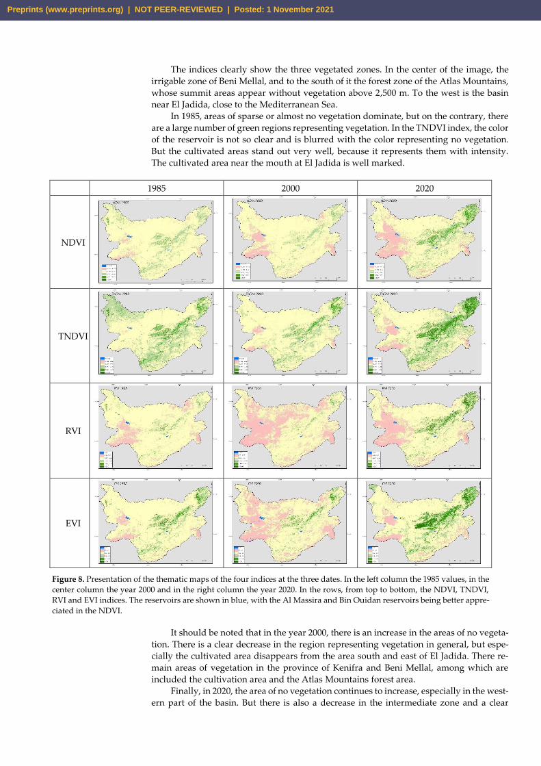
Figure 8 shows the results obtained. The year 2000 is the year with the smallest veg-

etated area, while 1985 is in an intermediate coverage and 2020 presents the maximum

coverage of the dates studied. The visual coincidence of the results of the four indexes is

highlighted. However, the TNDVI and EVI figures appear as those that best represent the

situation.


The indices clearly show the three vegetated zones. In the center of the image, the

irrigable zone of Beni Mellal, and to the south of it the forest zone of the Atlas Mountains,

whose summit areas appear without vegetation above 2,500 m. To the west is the basin

near El Jadida, close to the Mediterranean Sea.

In 1985, areas of sparse or almost no vegetation dominate, but on the contrary, there

are a large number of green regions representing vegetation. In the TNDVI index, the color

of the reservoir is not so clear and is blurred with the color representing no vegetation.

But the cultivated areas stand out very well, because it represents them with intensity.

The cultivated area near the mouth at El Jadida is well marked.

1985 2000 2020

NDVI

TNDVI

RVI

EVI

Figure 8. Presentation of the thematic maps of the four indices at the three dates. In the left column the 1985 values, in the

center column the year 2000 and in the right column the year 2020. In the rows, from top to bottom, the NDVI, TNDVI,

RVI and EVI indices. The reservoirs are shown in blue, with the Al Massira and Bin Ouidan reservoirs being better appre-

ciated in the NDVI.

It should be noted that in the year 2000, there is an increase in the areas of no vegeta-

tion. There is a clear decrease in the region representing vegetation in general, but espe-

cially the cultivated area disappears from the area south and east of El Jadida. There re-

main areas of vegetation in the province of Kenifra and Beni Mellal, among which are

included the cultivation area and the Atlas Mountains forest area.

Finally, in 2020, the area of no vegetation continues to increase, especially in the west-

ern part of the basin. But there is also a decrease in the intermediate zone and a clear


increase in the green surface and therefore in the vegetated area. The irrigable zone of the

middle section of the river increases in vegetation intensity and also in the forest zone.

In order to know the exact area of vegetation in each year, a histogram has been cal-

culated for each index of each year, using the histogram analysis function of SNAP. Thus,

the histograms of each year have been calculated to obtain the numerical information and

the pixels have been grouped in class. Figure 8 shows the histograms for the period 1985

- 2020 of the EVI index.

Figure 9. Histograms of the EVI index on the dates studied.

From the data of the histograms of the four indices, it has been possible to calculate

the areas of each class in each index, and therefore to know the vegetated area in each year

(tables 3 to 6).

Table 3. Area of each NDVI class in km2

1985 1990 1995 2000 2005 2010 2015 2020

< -0.324 75 83 48 54 64 147 157 86

-0.324 ~ -0.106 1,900 4,913 5,140 5,990 4,379 4,127 3,264 7,709

-0.106 ~ 0.101 33,300 30,382 30,341 30,315 31,178 30,643 30,630 25,118

0.101 ~ 0.344 2,683 2,522 2,458 1,691 2,372 2,982 3,684 4,171

0.344 ~ 0.551 119 180 93 30 86 180 335 924

> 0.551 4 1 1 1 1 1 9 72

Table 4. Area of each RVI class in km2

1985 1990 1995 2000 2005 2010 2015 2020

< 0.50 82 128 64 59 111 199 199 94

0.50 ~ 0.85 12143 21825 21185 24254 22387 18127 17059 17821

0.85 ~ 1.44 24207 14309 15200 12755 14004 17627 17985 16252

1.44 ~ 1.99 1433 1434 1400 940 1372 1729 2196 2454

1.99 ~ 2.45 139 307 189 56 161 315 444 775

> 2.45 77 78 43 17 45 83 198 682

Table 5. Area of each TNDVI class in km2

1985 1990 1995 2000 2005 2010 2015 2020

< 0.37 56 41 31 48 42 63 92 79

0.37 ~ 0.61 5409 12922 12696 16147 13365 10213 8062 12899

0.61 ~ 0.71 25901 19755 20147 17878 19684 21660 22791 16541

0.71 ~ 0.83 5437 3852 3888 3233 3717 4382 4746 5114

0.83 ~ 0.94 1247 1499 1307 769 1258 1742 2317 3148

> 0.94 30 12 10 5 13 20 73 298


Table 6. Area of each EVI class in km2

1985 1990 1995 2000 2005 2010 2015 2020

< 0.07 2183 13121 32521 21307 9710 3067 1258 1408

0.07 ~ 0.14 24858 16932 4213 11847 21365 24685 7702 12286

0.14 ~ 0.21 7602 5058 1277 3273 4271 5871 19696 15930

0.21 ~ 0.28 2793 2046 361 1323 1866 2905 4952 4084

0.28 ~ 0.35 1198 892 50 516 831 1304 2412 2889

> 0.35 97 396 24 180 403 613 2426 1848

Observing the four indices, despite their obvious differences, they are correlated with

each other and the representation in classes is similar, as in the case of 2020 for example

(Figure 10a). The most correlated indices are TNDVI and EVI (Figure 10b) whose relation-

ship between them presents a coefficient of determination of 0.9706.

Regarding the periodic series between 1985 and 2020 in the river basin, in the inter-

mediate period the vegetation area decreased and the null vegetation zone began to in-

crease. At present, this null zone continues to increase, but so does the vegetation area.

Figure 9 shows the distribution of EVI values, where values lower than 0.07 indicate arid

zones, while values higher than 0.14 indicate vegetated zones. In drought years, distribu-

tions are observed more pointed in the low values, while in favorable years the distribu-

tion loses pointing and widens the tails, indicating that although there are areas of aridity,

there are also areas with abundant vegetation.

Figure 10. A) Distribution of the surface area of the Oum Er Bia river basin in classes of the four vegetation indices

in 2020. B) Correlation between the TNDVI and EVI index.

3.2. Expansion of agriculture

The expansion of agriculture from satellite images in the middle basin of the river,

corresponding to the province of Tadla Azilal, is clustered around the towns of Beni Mel-

lal on the left bank and Beni Amir on the right bank, currently comprising an agricultural

area of about 4000 km2. The increase from 1985 to the present has not been what was ex-

pected in the initial irrigation plans (about 10,000 km2). In Figure 11a and 11b it can be

visually observed how the irrigated area has increased due to the increase in vegetated

area with high EVI values. The scrub and Mediterranean forest area appear in the moun-

tainous part of the Atlas and has also increased its vegetation density.


(a) 1985 (b) 2020

(c)

Figure 11. Variation of the cultivated area in the middle stretch of the river in the Beni-Mellal and Beni-Amir areas in (a) April

1985, Landsat-5 image; (b) April 2020, Landsat-8 image; (c) distribution of the area of the territory in the EVI values in the two

years considered from Landsat images obtained in Google Earth Engine.

Figure 11c presents the numerical values and surfaces for various classes of the index.

While the aridity zone has been maintained in these years, the first vegetation class has

decreased dramatically from 1985 to 2020, and this area has contributed to the increase of

the other classes of the index already related to the presence of vegetation.

In the Beni Amir environment, landscape change has been significant in this study

period.


a) b)

Figure 12. Detailed comparison of the area around the city of Beni Amir of the EVI index in (a) April 1985 and (b) April 2020.

Enlarged images of Figure 10.

The ranges of values of the EVI index make it possible to distinguish the cultivated

areas according to the existing vegetation. Figure 11a shows a regular distribution of fields

around the town of Beni-Amir, where regular mosaic farming was carried out in 1948,

interspersing plots of arable crops with woodland (mainly citrus) and fallow land [2]. At

that time, irrigation was about 134 km2 and was limited to water pumped from the river

in the absence of the regulation of the El Hansali reservoir. When it was transformed into

irrigated land with full availability of water with the construction of the reservoir and the

extension of the irrigation canals, the regular mosaic was lost as shown in Figure 11b; the

fallow land disappeared and became an area of varied herbaceous crops. In addition, new

cultivated areas of herbaceous crops are created with pivot irrigation to the west, destined

to forage plants for local use, whose circles are perfectly visible, some of which are larger

than a kilometer in diameter; in the northern zone other large extensions of crops have

also been created.

4. Discussion

Satellite images provide a temporal view of the planet's surface that is changeable

over the years, and remain as a record of a past time, allowing to elaborate studies in long

time series of changes in uses or natural changes [35]. The existence of the Landsat series

is an unquestionable utility in current studies, as well as the possibilities of processing in

large territories, being used by numerous published studies, such as Zadbagher et al. [36]

who studied the change of land use and land cover by Landsat images in Turkey; the

studies of forest changes by Banksota et al. [37]; the studies of temporal variations in wet-

lands by Kayastha et al. [38]. Specifically on agrarian issues, work has been developed all

over the planet, such as studies of abandonment of cultivated areas in the Caucasus [39],

studies on crop cycles in the Amazon in Brazil [40], or the spatio-temporal reconstruction

of the development of irrigation in Uzbekistan [41].

Vegetation indices have been used in the study of agricultural areas since they first

appeared, due to their economic importance. The first works with the first satellites that

came into service, such as studies of wheat growth using the LAI leaf area index [42],

water stress in wheat cultivation [43] and the effect of pest attacks on forests [44]. The

TNDVI index has shown its usefulness in studies in agricultural ecosystems and among

recent works, it has been used to study the sustainability of agriculture in Iraq using re-

mote sensing and geomatics techniques [45], monitoring carbon sequestration in orchards

[46], or spatiotemporal studies on aridity in the Punjab of Pakistan [47]. The use of EVI

has limitations due to the influence of relief and topography [48], where the presence of

shaded areas may give lower values of the index than would be appropriate. In our case,

since the agricultural area is in a plain, this problem does not exist. Many studies with the


EVI index have been performed with MODIS images [49] where index values were found

for an area of Matto Grosso in Brazil varying in the range of 0.20 to 0.65 for agricultural

areas, 0.25 to 0.50 for grasslands and scrublands and 0. 50 to 0.60 for forests; these values

are coincident with those obtained in our study, although in the agricultural zone of Tadla

Azilal the agricultural zones start at values of 0.15, at times when certain crops are in their

initial stages. These lower values are in agreement with those obtained by Chen et al. [50]

in cornfields in Mexico, where the minimum values were as low as 0.14 and the maximum

values exceeded 0.60. Actually, the minimum values are debatable without field work in

which vegetation measurements are made and the EVI index is estimated to observe the

values in the absence of vegetation; in that sense, the work of Tran et al. [51] points out

the value of 0.20 as the lower limit of vegetation when using Landsat-8 images. But the

study by Gosh et al. [52](2021) who made comparisons of EVI index between Sentinel-2

and Landsat-8 imagery in agricultural areas of India, indicates as low values as 0.10 for

fallow land, with normal values between 0.15 and 0.25, while values in cultivated land are

between 0.15 and 0.35 mostly. Therefore, we consider our class separation values to be

adequate for our study.

The changes that occurred in the agricultural extension in Tadla Azilal during the

20th century changed a territory dedicated to pastoralism and subsistence agriculture into

agricultural areas dedicated to extensive cultivation first from 1940 [2] as a result of the

French colonization plans. With independence of the country in 1956, the Moroccan new

government continued the policy of agricultural expansion in view of the agreements with

the European Union, continuing with the construction of reservoirs and new irrigable ar-

eas. At present, of the slightly more than 10,000 km2 planned for irrigable area in the mid-

dle section of the Oum Er Rbia valley, about 4,000 km2 have been deployed, and in the

total basin about 25,000 km2 are vegetated, either by crops or areas of scrubland and for-

ests in the Atlas area and the cultivated areas near the coast in El Jadida and Azemmour.

The changes in land use in Morocco are comparable to those in other Mediterranean

areas such as the Campo de Cartagena (Murcia, Spain), where a process of transformation

to irrigation has taken place with surface water inputs (although of smaller dimensions)

affecting about 200 km2. However, other agricultural territories suffered this transfor-

mation more than 1000 years ago in the Iberian Peninsula. The Huerta de Valencia was

transformed into irrigated land in the 10th century by the channeling of surface water

from the River Turia, as were the irrigated lands of the Segura in Murcia and Alicante

(Spain). The banks of the Júcar, however, are later and began in the 13th century and

ended in the 18th century as consolidated irrigation [53]. However, there is an important

difference between these areas, namely the great extent of agricultural transformations in

Morocco. While all the combined irrigated areas mentioned in Valencia and Murcia ac-

count for about 1,300 km2, in Tadla Azilal county there are already about 4,000 km2. In

addition, the extent of irrigation in Morocco, considering the other river basins, could con-

solidate up to 100,000 km2 if it reaches the maximum expected from the hydraulic con-

structions carried out in Morocco since the mid-twentieth century [4].

Regarding the usefulness of the vegetation indices in this case study, we consider the

TNDVI as the best index to evaluate the vegetation, mainly because it allows you not to

work with negative numbers, and because it highlights the vegetation better as seen in the

figures of the indices, since it is the only one in which the cultivated area near El Jadida

does not disappear. However, when the processing of the images with SNAP is long and

costly and requires sufficiently powerful computer equipment, its use would not be ad-

visable. In that sense, the use of the Google Earth Engine platform has the advantage of

having the data already calculated without having to locally process the information, but

it has the disadvantage that it only offers the EVI index for the moment (summer 2021)

and besides you cannot choose the images specifically. This index is also suitable espe-

cially in flat terrain, where there is no influence of topography. Contrast with field data is

necessary in future work to verify the minimum values of vegetated terrain.

5. Conclusions


The increase of the agricultural area in Morocco and specially in the Oum Er Rbia

river valley has been due to the availability of regulated water and the construction of

hydraulic works for its conduction to areas to expand the irrigation fields and increase

agricultural production. We evaluated by means of several vegetation indices applied to

satellite images, how the agricultural area has been changing from the 1980s to the pre-

sent, comparing for the first time the use of the Google Earth Engine with local processing

by SNAP software. We found that there are not differences in terms of the results ob-

tained, but the local downloading and processing of Landsat images is time-consuming

and the advantages of the cloud download and processing by Google is better if the need

is covered. The increase of agricultural area is important is the study site and has changed

from a production related to national demand to an intensive production for export to

European Union.

Author Contributions: Conceptualization, J. Soria; Formal analysis, M. Adell and J.A. Domínguez-

Gómez; Investigation, M. Adell and J. Soria; Methodology, M. Adell and J.A. Domínguez-Gómez;

Writing – original draft, J. Soria; Writing – review & editing, J.A. Domínguez-Gómez. All authors

have read and agreed to the published version of the manuscript.

Funding: This research received no external funding.

Data Availability Statement: Landsat satellite images are downloaded from USGS server.

Conflicts of Interest: The authors declare no conflict of interest.

Appendix A

The appendix is an optional section that can contain details and data supplemental

to the main text—for example, explanations of experimental details that would disrupt

the flow of the main text but nonetheless remain crucial to understanding and reproduc-

ing the research shown; figures of replicates for experiments of which representative data

is shown in the main text can be added here if brief.

References

1. Schilling, J.; Freier, K.P.; Hertig, E.; Scheffran, J. Climate change, vulnerability and adaptation in North Africa with focus on

Morocco. Agr. Ecosyst. Environ. 2012, 156, 12-26. https://doi.org/10.1016/j.agee.2012.04.021

2. Nemmaoui, A.; Lorca, A.G. La irrigación en Marruecos: El Caso de Tadla-Azilal. Cuadernos Geogr. 2009, 44, 113-132. Available

online: https://www.redalyc.org/articulo.oa?id=17111823005 (Accessed on 10-sept-2021)

3. El Orfi, T.; El Ghachi, M.; Lebaut, S. Contributions of remote sensing in the diachronic study of the spatial and temporal evolu-

tion of the Ahmed El Hansali dam water reservoir from 2002-03 to 2018-19. In E3S Web of Conferences 2020, 183, 02004.

https://doi.org/10.1051/e3sconf/202018302004

4. Conseil Général du Développement Agricole. Atlas de l’Agriculture marocaine. 2nd edition. Ministère de l’Agriculture et de la

Pêche Maritime. Royaume du Maroc, 2009, pp. 56. Available online: https://www.agriculture.gov.ma/fr/publications/atlas-de-

lagriculture-marocaine (accessed 30 September 2021).

5. Williams, D.L.; Goward, S.; Arvidson, T. Landsat. Photogramm. Eng. Rem. S. 2006, 72(10), 1171-1178.

https://doi.org/10.14358/PERS.72.10.1171

6. Townshend, J.R.G.; Goff, T.E.; Tucker, C.J. Multitemporal dimensionality of images of normalized difference vegetation index

at continental scales. IEEE T. Geosci. Remote 1985, GE-23(6), 888-895. https://doi.org/10.1109/TGRS.1985.289474

7. Henricksen, B. L.; Durkin, J. W. Growing period and drought early warning in Africa using satellite data. Int. J. Remote Sens.

1986, 7(11), 1583-1608. https://doi.org/10.1080/01431168608948955

8. Singhf, S.M. Vegetation index and possibility of complementary parameters from AVHRR/2. Int. J. Remote Sens. 1986, 7(2), 295-

300. https://doi.org/10.1080/01431168608954685

9. Gao, B.C. Normalized difference water index for remote sensing of vegetation liquid water from space. In Imaging Spectrometry,

International Society for Optics and Photonics, 1995, pp. 225-236. https://doi.org/10.1117/12.210877

10. McFeeters, S.K. The use of the normalized difference water index (NDWI) in the delineation of open water features. Int. J. Remote

Sens. 1996, 17(7), 1425-1432. https://doi.org/10.1080/01431169608948714

11. Dowdeswell, J.A.; Gorman, M.R.; Macheret, Y.Y., Moskalevsky, M.Y., Hagen, J.O. Digital comparison of high resolution

sojuzkarta KFA-1000 imagery of ice masses with Landsat and SPOT data. Ann. Glaciol. 1993, 17, 105-112.

https://doi.org/10.3189/s0260305500012684

12. Toll, D.L. An evaluation of simulated Thematic Mapper data and Landsat MSS data for discriminating suburban and regional

land use and land cover (USA). Photogramm. Eng. Rem. S. 1984, 50(12), 1713-1724.


13. Otterman, J.; Tucker, C.J. Satellite measurements of surface albedo and temperatures in semi- desert. J. Clim. App. Meteorol. 1985,

24(3), 228-235. https://doi.org/10.1175/1520-0450(1985)024<0228:SMOSAA>2.0.CO;2

14. Rouse, J.W; Haas, R.H.; Scheel, J.A.; Deering, D.W. 'Monitoring Vegetation Systems in the Great Plains with ERTS.' Proceedings,

3rd Earth Resource Technology Satellite (ERTS) Symposium 1974, 1, p. 48-62. Available online: https://ntrs.nasa.gov/cita-

tions/19740022614 (accessed 9 October 2021).

15. Richardson, A.J.; Wiegand, C.L. Distinguishing vegetation from soil background information. Photogramm. Eng. Rem. S. 1977,

43(12), 1541-1552.

16. Senseman, G.M.; Bagley, C.F.; Tweddale, S.A. Correlation of rangeland cover measures to satellite-imagery-derived vegetation

indices. Geocarto Int. 1996, 11(3), 29-38. https://doi.org/10.1080/10106049609354546

17. Huete, A.R. A soil-adjusted vegetation index (SAVI). Remote Sens. Environ. 1988, 25(3), 295-309. https://doi.org/10.1016/0034-

4257(88)90106-X

18. Richardson, A.J. Wiegand, C.L. Distinguishing vegetation from soil background information. Photogramm. Eng. Rem. S. 1977,

43(12), 1541-1552.

19. Huete, A.R.; Liu, H.Q.; Batchily, K.V.; Van Leeuwen, W.J.D.A. A comparison of vegetation indices over a global set of TM

images for EOS-MODIS. Remote Sens. Environ. 1997, 59(3), 440-451. https://doi.org/10.1016/S0034-4257(96)00112-5

20. Echakraoui, Z.; Boukdir, A.; Aderoju, O.; Zitouni, A.; Dias, A.G. The climate changes in the sub-basin of the Oum Er Rbia central

and the impact on the surface waters. In E3S Web of Conferences 2018, 37, 03003.

21. Ouatiki, H.; Boudhar, A.; Ouhinou, A.; Arioua, A.; Hssaisoune, M.; Bouamri, H.; Benabdelouahab, T. Trend analysis of rainfall

and drought over the Oum Er-Rbia River Basin in Morocco during 1970–2010. Arabian J Geosci. 2019, 12(4), 128.

22. Strohmeier, S.; López, P.; Haddad, M.; Nangia, V.; Karrou, M.; Montanaro, G.; Boudhar, A.; Linés, C.; Veldkamp, T.; Sterk, G.

Surface Runoff and Drought Assessment Using Global Water Resources Datasets - from Oum Er Rbia Basin to the Moroccan

Country Scale. Water Resour. Manage. 2020, 34, 2117–2133. https://doi.org/10.1007/s11269-019-02251-6

23. Tahiri, A.; Amraoui, F.; Sinan, M. Remote sensing, GIS, and Fieldwork Studies to assess and valorize groundwater resources in

the springs area of Oum-Er-Rbia (Moroccan Middle Atlas). Groundwater for Sustainable Development 2020, 11, 100440.

https://doi.org/10.1016/j.gsd.2020.100440.

24. Van Straaten, C. Regional modeling of water stress Irrigation water requirement meets water availability in the Oum er Rbia

basin. MSc thesis. Utrecht, NL, 2017. Retrieved from http://dspace.library.uu.nl/handle/1874/352929 (accessed on 10 October

2021).

25. De Lamotte, D.; Leturmy, P.; Missenard, Y.; Khomsi, S.; Ruiz, G.; Saddiqi, O.; Guillocheau, F.; Michard, A. Mesozoic and Ceno-

zoic vertical movements in the Atlas system (Algeria, Morocco, Tunisia): An overview. Tectonophysics 2009, 475(1), 9–28.

https://doi.org/10.1016/j.tecto.2008.10.024

26. Sousa, R.; Varandas, S.; Teixeira, A.; Ghamizi, M.; Froufe, E.; Lopes-Lima, M. Pearl mussels (Margaritifera marocana) in Mo-

rocco: Conservation status of the rarest bivalve in African fresh waters. Sci. Tot. Environ. 2016, 547, 405-412.

https://doi.org/10.1016/j.scitotenv.2016.01.003

27. El Haibi, H.; EL Hadi, H.; Tahiri, A.; Martínez Poyatos, D.; Gasquet, D.; Pérez-Cáceres, I.; González Lodeiro, F., Mehdioui, S.

Geochronology and isotopic geochemistry of Ediacaran high-K calc-alkaline felsic volcanism: An example of a Moroccan peri-

gondwanan (Avalonian?) remnant in the El Jadida horst (Mazagonia). J. African Earth Sci. 2020, 163, 103669.

https://doi.org/10.1016/j.jafrearsci.2019.103669

28. Paaza, N.; Larocque, M.; Herrera, J. Modèle de circulation hydrogéologique au niveau de l’aquifère plioquaternaire de Settat

(Maroc): étude hydrogéochimique. Rev. Sci. Eau 2018, 31(4), 401–414. https://doi.org/10.7202/1055597ar

29. Daki, Y.; Lachgar, R.; Zahour, G. Étude Hydroclimatique du bassin du haut Oum Er Rbia [Hydroclimatic study of high Oum

Er Rbia basin]. Int. J. Innov. Appl. Studies 2015, 12(3), 644.

30. Yjjou, M.; Bouabid, R.; El Hmaidi, A.; Essahlaoui, A. Caractérisation topographique et climatique via le SIG du bassin versant

du haut Oum Er-Rbia en amont du barrage El Hansali (SW du Moyen Atlas, Maroc). Journal of Hydrocarbons Mines and Environ-

mental Research 2012, 3, 104-109. https://doi.org/10.1007/s11269-019-02251-6

31. Funnell, D.C.; Binns, J.A. Irrigation and rural development in Morocco. Land Use Policy 1989, 6(1), 43-52.

32. Dwarakish, G. S.; Nithyapriya, B. Application of soft computing techniques in coastal study–A review. J. Ocean Eng. Sci. 2016,

1(4), 247-255. https://doi.org/10.1016/j.joes.2016.06.004

33. Pettorelli, N. The normalized difference vegetation index. Oxford University Press: Oxford, UK, 2013.

34. Borra, S.; Thanki, R.; Dey, N. Satellite image analysis: clustering and classification. Springer: Singapore, 2019.

35. Hegazy, I.R.; Kaloop, M.R. Monitoring urban growth and land use change detection with GIS and remote sensing techniques

in Daqahlia governorate Egypt. Int. J. Sust. Built Environ. 2015, 4(1), 117-124. https://doi.org/10.1016/j.ijsbe.2015.02.005

36. Zadbagher, E.; Becek, K.; Berberoglu, S. Modeling land use/land cover change using remote sensing and geographic information

systems: case study of the Seyhan Basin, Turkey. Environ. Monit. Assess. 2018, 190(8), 1-15. https://doi.org/10.1007/s10661-018-

6877-y

37. Banskota, A.; Kayastha, N.; Falkowski, M.J.; Wulder, M.A.; Froese, R.E.; White, J. C. Forest monitoring using Landsat time series

data: A review. Canadian J. Remote Sens. 2014, 40, 362-384. https://doi.org/10.1080/07038992.2014.987376

38. Kayastha, N., Thomas, V., Galbraith, J., & Banskota, A. Monitoring wetland change using inter-annual Landsat time-series data.

Wetlands 2012, 32(6), 1149-1162. https://doi.org/10.1007/s13157-012-0345-1

39. Yin, H.; Prishchepov, A.V.; Kuemmerle, T.; Bleyhl, B.; Buchner, J.; Radeloff, V. C. Mapping agricultural land abandonment from

spatial and temporal segmentation of Landsat time series. Remote Sens. Environ. 2018, 210, 12-24.

https://doi.org/10.1016/j.rse.2018.02.050


https://ntrs.nasa.gov/citations/19740022614

https://ntrs.nasa.gov/citations/19740022614

http://dspace.library.uu.nl/handle/1874/352929

40. Dutrieux, L.P.; Jakovac, C.C.; Latifah, S.H.; Kooistra, L. Reconstructing land use history from Landsat time-series: Case study

of a swidden agriculture system in Brazil. Int. J. Appl. Earth Obs. 2016, 47, 112-124. https://doi.org/10.1016/j.jag.2015.11.018

41. Edlinger, J.; Conrad, C.; Lamers, J.P.A.; Khasankhanova, G.; Koellner, T. Reconstructing the Spatio-Temporal Development of

Irrigation Systems in Uzbekistan Using Landsat Time Series. Remote Sens. 2012, 4, 3972-3994. https://doi.org/10.3390/rs4123972

42. Pollock, R.B.; Kanemasu, E.T. Estimating leaf-area index of wheat with Landsat data. Remote Sens. Environ. 1979, 8(4), 307-312.

https://doi.org/10.1016/0034-4257(79)90030-0

43. Jackson, R.D.; Slater, P.N.; Pinter Jr, P.J. Discrimination of growth and water stress in wheat by various vegetation indices

through clear and turbid atmospheres. Remote Sens. Environ. 1983, 13(3), 187-208. https://doi.org/10.1016/0034-4257(83)90039-1

44. Nelson, R.F. Detecting forest canopy change due to insect activity using Landsat MSS. Photogramm. Eng. Rem. S. 1983, 49(9),

1303-1314.

45. El Mewafi, M.; Kedy, S.K.; Elnaggar, A.A. Changes of Land Cover in Diwaniyah Governorate and their Impact on Agricultural

Sustainability by Using Geomatics Techniques (Dept. C (Public Works)). Bulletin of the Faculty of Engineering. Mansoura Univer-

sity 2020, 40(3), 19-36. https://doi.org/10.21608/bfemu.2020.101860

46. Uttaruk, Y.; Laosuwan, T. Carbon sequestration assessment of the orchards using satellite data. J. Ecol. Eng. 2017, 18(1). DOI

10.12911/22998993/66257

47. Siddiqui, S.; Javid, K. Spatio-temporal analysis of aridity over Punjab Province, Pakistan using remote sensing techniques. Int.

J. Econ. Environ. Geol. 2019, 9, 1-10. https://doi.org/10.46660/ijeeg.Vol0.Iss0.0.19

48. Matsushita, B.; Yang, W.; Chen, J.; Onda, Y.; Qiu, G. Sensitivity of the Enhanced Vegetation Index (EVI) and Normalized Dif-

ference Vegetation Index (NDVI) to Topographic Effects: A Case Study in High-density Cypress Forest. Sensors 2007, 7, 2636-

2651. https://doi.org/10.3390/s7112636

49. Arvor, D.; Jonathan, M.; Meirelles, M.S.P.; Dubreuil, V.; Durieux, L. Classification of MODIS EVI time series for crop mapping

in the state of Mato Grosso, Brazil. Int. J. Remote Sens. 2011, 32, 7847-7871, DOI: 10.1080/01431161.2010.531783

50. Chen, P.Y.; Fedosejevs, G.; Tiscareno-Lopez, M.; Arnold, J.G. Assessment of MODIS-EVI, MODIS-NDVI and VEGETATION-

NDVI composite data using agricultural measurements: An example at corn fields in western Mexico. Environ. Monit. Asses.

2006, 119, 69-82. https://doi.org/10.1007/s10661-005-9006-7

51. Tran, T.V.; Tran, D.X.; Nguyen, H.; Latorre-Carmona, P.; Myint, S.W. Characterising spatiotemporal vegetation variations using

LANDSAT time-series and Hurst exponent index in the Mekong River Delta. Land Degrad. Dev. 2021, 32, 3507– 3523.

https://doi.org/10.1002/ldr.3934

52. Ghosh, S.; Behera, D.; Jayakumar, S.; Das, P. Comparison of Sentinel-2 Multispectral Imager (MSI) and Landsat 8 Operational

Land Imager (OLI) for Vegetation Monitoring. In Spatial Modeling in Forest Resources Management. Environmental Science and

Engineering. Shit P.K.; Pourghasemi H.R.; Das P.; Bhunia G.S. Eds; Springer: Swiss. 2021. https://doi.org/10.1007/978-3-030-

56542-8_7

53. Glick, T.F.; Kirchner, H. Hydraulic Systems and Technologies of Islamic Spain: History and Archaeology. In: Working with Water

in Medieval Europe. Brill: The Hague, NL, 2000; pp. 267–329. https://doi.org/10.1163/9789047400110_011


Date post:	21-Dec-2021
Category:	Documents
Upload:	others
View:	0 times
Download:	0 times

Monitoring of forty years of agricultural expansion in the ...

Documents