Monitoring of observation errors in the assimilation of satellite

ozone data

Ivanka Stajner,1 Nathan Winslow,2 Richard B. Rood,3 and Steven Pawson4

Global Modeling and Assimilation Office, NASA Goddard Space Flight Center, Greenbelt, Maryland, USA

Received 28 August 2003; revised 12 December 2003; accepted 28 January 2004; published 25 March 2004.

[1] Ozone observations from the Solar Backscatter UltraViolet/2 (SBUV/2) instrumentsand/or the Earth Probe Total Ozone Mapping Spectrometer (EP TOMS) have beenassimilated in near-real time at NASA’s Data Assimilation Office (DAO) since January2000. The ozone data assimilation system was used as a tool for detecting andcharacterizing changes in the observation errors. The forecast model captures thegeophysical variability. A change in the observed-minus-forecast (O-F) residuals, whichare defined as differences between the incoming ozone observations and the collocatedshort-term model forecast, indicates a change in the assimilation system. If the model andthe statistical analysis scheme are stable, then it points to a modification in instrumentcharacteristics or a retrieval algorithm. However, sometimes a change in the ozone O-Fresiduals is caused by differences in the availability of the meteorological observations ormodifications in the meteorological assimilation system whose winds are used to drive theozone transport model. The O-F residuals are routinely produced and monitored in theassimilation process. Using examples from the NOAA 14 and NOAA 16 SBUV/2instruments, and the EP TOMS, we demonstrate that the monitoring of time series of O-Fresidual statistics is an effective, sensitive, and robust method for identifying time-dependent changes in the observation-error characteristics of ozone. In addition, the dataassimilation system was used to assist in the validation of updated calibration coefficientsfor the NOAA 14 SBUV/2 instrument. This assimilation-based monitoring work is beingextended to ozone data from instruments on new satellites: Environmental satellite(Envisat), Earth Observing System (EOS) Aqua, and EOS Aura. INDEX TERMS: 0341

Atmospheric Composition and Structure: Middle atmosphere—constituent transport and chemistry (3334);

3337 Meteorology and Atmospheric Dynamics: Numerical modeling and data assimilation; 3360 Meteorology

and Atmospheric Dynamics: Remote sensing; 3394 Meteorology and Atmospheric Dynamics: Instruments and

techniques; KEYWORDS: assimilation, satellite, ozone data

Citation: Stajner, I., N. Winslow, R. B. Rood, and S. Pawson (2004), Monitoring of observation errors in the assimilation of satellite

ozone data, J. Geophys. Res., 109, D06309, doi:10.1029/2003JD004118.

1. Introduction

[2] Satellite borne instruments provide a wealth of dataabout the Earth’s atmosphere with a continuous andoften near-global coverage. A few examples are theTIROS Operational Vertical Sounder (TOVS) [Smith etal., 1979], the Atmospheric Infrared Sounder (AIRS)[Aumann et al., 2003], and the Total Ozone MappingSpectrometer (TOMS) [McPeters et al., 1998]. Satellitedata are core input data sets with ever increasingimportance for modern data assimilation systems. These

systems are used to provide estimates and forecasts ofthe state of the atmosphere. Improvements in the avail-ability, accuracy, and assimilation of satellite data aremajor factors contributing to the improvement in theaccuracy of weather forecasts [Hollingsworth et al.,2003]. Careful monitoring of the errors in the satellitedata is critical for their optimal usage within assimilationsystems. Improvements in understanding of satellite dataand their errors contribute to increased accuracy ofweather and atmospheric constituent forecasts, potentiallyenable improvements in forecast models, and can ulti-mately lead to a better understanding of the underlyinggeophysical processes.[3] Validation of retrieved data from satellite borne in-

strument measurements is a difficult task that can becomplicated by many factors [e.g., Fetzer et al., 2003].For newer instruments with high spectral and fine spatialresolution, such as AIRS, the large data volume makes thevalidation a very demanding task. Thus development anduse of sensitive, automated procedures that can aid in the

JOURNAL OF GEOPHYSICAL RESEARCH, VOL. 109, D06309, doi:10.1029/2003JD004118, 2004

1Science Applications International Corporation, Beltsville, Maryland,USA.

2Decision Systems Technologies, Inc., Rockville, Maryland, USA.3Earth and Space Data Computing Division, NASA Goddard Space

Flight Center, Greenbelt, Maryland, USA.4Goddard Earth Sciences and Technology Center, University of

Maryland Baltimore County, Baltimore, Maryland, USA.

Copyright 2004 by the American Geophysical Union.0148-0227/04/2003JD004118$09.00

D06309 1 of 12

monitoring and validation of retrieved satellite data isdesirable.[4] Traditionally, retrieved data products from satellite

instruments have been validated in several ways. Forexample, algorithms used for their derivation are checkedusing synthetic and test input data [e.g., Froidevaux et al.,1996]. Raw satellite-instrument radiances are monitored forabrupt changes and longer-term drifts. Zonal means ofretrieved geophysical fields may be compared with thezonal means of model or assimilated fields [e.g., Gille etal., 1996]. The retrieved products are compared to data fromthe same instrument and from different instruments [e.g.,Froidevaux et al., 1996; Remsberg et al., 2002]. Thesecomparisons are typically done using collocated data thatare taken within certain distance and time from each other.The role of the collocation is to minimize the underlyingtemporal and spatial variability of geophysical fields. How-ever, this dynamical variability is explicitly represented bythe assimilated geophysical fields. This is one of theadvantages of using assimilated fields in the validation ofsatellite data products.[5] Data assimilation can contribute to validation of

satellite data products. This approach capitalizes on theinherent ability of assimilation to handle large data volumes,often in near-real time, and facilitate a rapid feedback aboutthe data quality to the instrument teams. Fields produced byassimilation into global models can provide a precise timeand spatial collocation with every satellite measurement.The global nature of these fields allows application ofaveraging kernels, and production of a validation data setwhose spatial representation is suitable for comparison withretrieved data. This is particularly important for instrumentsproviding total or weighted columns of chemical constitu-ents [e.g., Rodgers and Connor, 2003].[6] Data assimilation techniques have been applied to

monitoring and validation of observation errors. The frame-work was established by Hollingsworth et al. [1986], whodemonstrated the value of data assimilation systems formonitoring of the performance of the radiosonde network.Long-term monitoring in meteorological reanalyses is pre-sented by Uppala [1997], who demonstrated clear changesin system O-F biases for the radiosonde record and 1d-varretrievals of TOVS data over the period 1979–1993. Piterset al. [1999] validated Global Ozone Monitoring Experi-ment (GOME) total column ozone observations using theAssimilation Model at the Royal Dutch MeteorologicalInstitute (KNMI). They evaluated a random error in GOMEand found a systematic error depending on the viewingdirection. Similar approaches have also been successfullyused in calibration and validation of other types of satelliteobservations. Stoffelen [1999] used wind fields from anumerical weather prediction model in calibration of theEuropean Remote Sensing Satellite (ERS) scatterometers.This calibration is beneficial to the ERS geophysical prod-uct (the surface wind field over oceans). It is used formonitoring of the ERS scatterometers, and it can detectsudden instrument anomalies within six hours. Atlas et al.[1999] performed geophysical validation of NASA scatter-ometer (NSCAT) data sets. They compared NSCAT datawith collocated wind data from ships, buoys, other satellitedate, and reference analyzed fields produced by assimilationof other data. These comparisons yielded estimates of the

error characteristics of NSCAT data. When NSCAT datawere assimilated, they found improvements in the resultinganalysis and forecast fields.[7] In this paper we apply data assimilation techniques to

monitoring of the error characteristics of satellite ozonedata. In section 2 we give a brief overview of the dataassimilation system and of the techniques for monitoring ofobservation errors that are used throughout the paper.Subsequent sections contain examples from near-real timemonitoring of errors in ozone data from three satellite-borneozone instruments: the NOAA 14 Solar Backscatter Ultra-violet/2 (SBUV/2) instrument, the Earth Probe (EP) TOMS,and the NOAA 16 SBUV/2 instrument. In section 3 wefocus on the changes in the NOAA 14 SBUV/2 ozoneprofile data error characteristics, and their impact on theassimilated ozone fields. Monitoring of total column ozonefrom EP TOMS and NOAA 16 SBUV/2 instruments isgiven in section 4. This section also includes examples ofdiscontinuities in the O-F residual statistics due to changesin the meteorological data assimilation system. The use ofglobal and regional statistics of the O-F residuals is illus-trated by several examples of algorithm and calibrationmodifications in the NOAA 16 SBUV/2 ozone profiles insection 5. Discussion of the results and plans for futurework are given in section 6.

2. Background

[8] Data assimilation [Daley, 1991] provides a frame-work for combining available observational atmosphericdata, along with their error characteristics, with a modelprediction and its error characteristics to obtain the bestestimate of the true atmospheric fields. This process yieldsanalyzed or assimilated fields. In the sequential ozoneassimilation process used in this paper (see Figure 1) themodel transfers information from previous observationaltimes to the current synoptic time. At the new synoptictime the model estimated field is updated with observa-tions. In regions with dense observations the modelestimate is, perhaps, changed substantially. In regions with

Figure 1. Schematic diagram of the ozone assimilationsystem with the major components and the data flow.

D06309 STAJNER ET AL.: MONITORING OF OZONE DATA BY ASSIMILATION

2 of 12

D06309

sparse, or no, observations the estimate of the atmosphericfield is largely determined by the model prediction. Astatistical analysis scheme is used to produce an analysisfield by combining the forecast field with the observationsvalid at this time according to their error characteristics.The cycle is then repeated. The forecast model can also beused to provide forecast fields for several days in advance.Data assimilation has been used successfully in numericalweather prediction, and increasingly also for obtainingdistributions of atmospheric chemical constituents [e.g.,Austin, 1992; Fisher and Lary, 1995; Long et al., 1996;Levelt et al., 1998; Eskes et al., 1999; Khattatov et al.,2000; Menard et al., 2000; Elbern and Schmidt, 2001;Stajner et al., 2001; Struthers et al., 2002; Dethof andHolm, 2002; Eskes et al., 2003].[9] An integral part of the data assimilation process is the

computation of differences between the observations andthe collocated model predictions of these quantities

wo � Hwf ; ð1Þ

where wo is the vector of all the observations available at asingle analysis time, H is the matrix of the observationoperator, and wf is the vector of the model forecast on theanalysis grid. These differences are the vectors of theobserved-minus-forecast (O-F) residuals, and they allow usto evaluate how consistent the observations are with ourunderstanding of the atmosphere as described by theforecast model. Note that the observation error consists ofthe measurement or retrieval error and the representative-ness error due to variability of the true field at scales that areunresolved by the discrete model. An O-F residual equalsthe difference between the observation error and the error inthe forecast of the observed quantity. Thus the statistics ofO-F residuals provide information about the observationand forecast errors. The O-F statistics are used extensivelyin data assimilation to monitor error characteristics andestimate error model parameters. For examples of theirapplication in constituent data assimilation, see Menard etal. [2000] and Menard and Chang [2000]. Under theassumption that the forecast model does not change, and itserror characteristics are constant in time, the differences inthe time series of the O-F statistics are due to changes in theobservation error characteristics. This approach that uses theforecast as a standard against which observations arecompared has inherent advantages and disadvantages dueto the underlying properties of assimilated fields. Advan-tages are that the forecast takes into account realisticgeophysical variability of the true fields, and that globalforecasts provide precise collocation with any observation.A disadvantage is that spatial and temporal variability offorecast errors complicates partitioning of the variability inO-Fs into the variability in forecast and observation errors,respectively. Implications for this work will be discussedbelow.[10] This study uses near-real-time O-F residuals pro-

duced by the operational Goddard Earth Observing Sys-tem (GEOS) ozone assimilation system [Riishøjgaard etal., 2000; Stajner et al., 2001]. The assimilated ozonefields agree well with independent high quality ozonedata. See Stajner et al. [2001] for some examples of thecomparisons of assimilated ozone against WMO ozone

sondes and Halogen Occultation Experiment (HALOE)[Bruhl et al., 1996]. In the initial configuration of thenear-real time ozone assimilation system, the EP TOMStotal column ozone [McPeters et al., 1998] and theNOAA 14 SBUV/2 instrument ozone profiles [Bhartiaet al., 1996] were assimilated into a tracer transport modelbetween January 2000 and April 2001. During April andMay 2001 EP TOMS total column ozone and NOAA 16SBUV/2 profile observations were assimilated. OnlyNOAA 16 SBUV/2 ozone total column and profileobservations were assimilated from May 2001. The tracertransport model [Lin and Rood, 1996], which was used topredict ozone, was driven by the assimilated wind fieldsfrom the version 3 of the GEOS Data Assimilation System(DAS). Note that several operational changes were intro-duced into GEOS-3 during this period: their impacts willbe discussed below.[11] The GEOS ozone assimilation system produces time

series of O-F statistics. We routinely monitor these timeseries for abrupt changes. We use global and regional meanand root-mean square (RMS) of O-F residuals for each datatype. For profile observations these statistics are computedfor each level. Another global statistic that we use in themonitoring is c2, defined as follows. If the errors in wo andwf are mutually uncorrelated Gaussian-distributed randomvectors with mean 0 and covariances P and R, respectively,then the O-F residuals wo � Hwf are Gaussian distributedwith the mean 0 and the covariance matrix HPHT + R. Therandom variable

z ¼ wo � Hwf� �T

HPHT þ R� ��1

wo � Hwf� �

; ð2Þ

then has the c2 distribution with p degrees of freedom,where p is the number of observations (dimension of wo) atone analysis time. The mean of z is p and the variance is 2p.The mean of the normalized variable z/p is 1. Note that therepresentativeness error for TOMS total column data, whosefootprint is smaller than the analysis model grid, is includedas an additive component in the model used to evaluate R[Stajner et al., 2001]. The SBUV footprint is comparable tothe horizontal resolution of the analysis grid: thus the SBUVrepresentativeness error need not be modeled explicitly.Initially, the c2 was monitored to check how consistent theassumed error covariance models are with the realizations ofthe O-F residuals. However, we found that c2 is alsoconvenient for detecting changes in the observation errorcharacteristics (as will be illustrated in section 5).

3. NOAA 14 Solar Backscattered Ultraviolet//2(SBUV//2) Ozone Profiles

[12] Ozone profiles retrieved from NOAA 14 SBUV/2instrument measurements and TOMS total ozone columndata were assimilated in near-real time into the GEOS ozonesystem during the period between January 2000 and April2001. The SBUV/2 instrument data are reported as partialozone columns in 12 layers [Bhartia et al., 1996]. Each ofthe layers 2 to 11 is �5 km thick. Ozone partial columnsfrom layers 3 (63–126 hPa) to 12 (0–0.25 hPa) areassimilated in our system [Stajner et al., 2001]. In thissection we focus on two examples of changes in NOAA 14SBUV/2 error characteristics that can be seen from statistics

D06309 STAJNER ET AL.: MONITORING OF OZONE DATA BY ASSIMILATION

3 of 12

D06309

of O-F residuals. We also examine impacts of changes in theformulation of the forecast model.

3.1. Features of the Data

[13] In order to evaluate temporal changes in the incomingSBUV/2 data we examine time series of statistics of O-Fresiduals. An example of the time series of the daily globalmean of O-F residuals for NOAA 14 SBUV/2 in the layer 5,between 16 and 32 hPa, is shown by the solid line in Figure 2.For reference, an average of SBUVobservations in this layeris�60 to 70 DU. Throughout the O-F mean time series thereis a typical day-to-day variability of �0.5 DU. However,there is a sharp increase on March 31, 2000 (mark ‘‘A’’ inFigure 2). The forecast model did not change in any way onthat day, but the calibration of the SBUV/2 instrument wasmodified. After the SBUV instrument team reexamined thecalibration coefficients, they derived updated coefficientsand reprocessed the data (M. Deland and D. McNamara,personal communication, 2000). We used the reprocessedSBUV/2 data in a short assimilation run, and the change inthe global mean O-F value on March 31 was reduced. Theselater calibration coefficients were operationally implementedby NOAA on August 8, 2000, when the mean of O-Fresiduals slightly decreases (mark ‘‘V’’ in Figure 2).[14] The second feature that stands out in the time series

of the mean of O-F residuals in Figure 2 is the increase inNovember 2000 between marks ‘‘B’’ and ‘‘C’’. This periodcoincides with the changes in the NOAA 14 SBUV/2instrument grating positions. When a grating positionchanges, the wavelength at which the measurement is madediffers from the nominal wavelength, and the actual wave-length is also reported with less accuracy. The wavelengthshift to a less optimal region of the spectrum, together witha less accurate knowledge of the actual wavelengths atwhich measurements are made, can increase the errors inthe ozone retrieval from SBUV data. The larger O-Fresiduals indicate that there was indeed a change in the

quality of the SBUV/2 data simultaneous with the gratingposition changes.

3.2. Sensitivity to Forecast Model

[15] Next, we examine how robust are features in the timeseries of the O-F residual statistics to changes in theformulation of the forecast model. The time series of theglobal mean O-F residuals for NOAA 14 SBUV/2 data inlayer 5 from an ozone assimilation into a modified ozoneforecast model is shown by the dotted line in Figure 2. Thismodel is driven by winds from a prototype of the version 4 ofGEOS meteorological assimilation, and it includes a chem-istry scheme with parameterized ozone production and lossrates [Fleming et al., 2001], where production rates wereadjusted so that the quotient of production and loss rates inthe upper stratosphere agrees with an ozone climatologybased on SBUV data [Langematz, 2000]. In contrast, theoperational assimilation driven by GEOS-3 fields (solid linein Figure 2) does not include any chemistry, only the ozonetransport, in the forecast model. Another difference betweenthe operational GEOS-3 and prototype GEOS-4 meteoro-logical systems is that the configuration of the operationalsystem was changed a couple of times during year 2000, buta fixed version of the prototype GEOS-4 system was usedfor the entire year. The largest contribution to the meandifferences between observations and forecasts comes fromthe tropical region. Both, upwelling and horizontal mixingreduce the ozone concentration in the SBUV/2 layer 5, justbelow the absolute mixing ratio peak near 10 hPa in thetropics. In the chemical parameterization, which is includedin GEOS-4 driven ozone assimilation, there is net ozoneproduction in this region. Thus the mean differencesbetween observations and forecast in SBUV/2 layer 5 aresmaller by �1.5 DU in the GEOS-4 driven assimilation.Comparisons of GEOS-4 driven assimilations with andwithout chemical parameterizations for the year 1998 indi-cate that �1 DU of this mean difference in SBUV/2 layer 5

Figure 2. Time series of daily global mean of NOAA 14 SBUV/2 O-F residuals in Umkehr layer 5 foroperational SBUV/2 data (solid line) is shown for the system driven by GEOS-3 winds. The samequantity from the ozone assimilation driven by winds from a prototype GEOS-4 system, and includingparameterized ozone chemistry is shown by the dotted line. Note the sharp jump near the mark ‘‘A’’exceeding the typical day-to-day variability followed by a downward trend in the mean of O-F residuals.This feature is coincident with the instrument calibration change on March 31. Near the mark ‘‘A’’ thesame quantity is shown for assimilation driven by GEOS-3 winds and using reprocessed SBUV/2 data(line with squares). An increase between marks ‘‘B’’ and ‘‘C’’ coincides with a change in the gratingposition of the instrument.

D06309 STAJNER ET AL.: MONITORING OF OZONE DATA BY ASSIMILATION

4 of 12

D06309

O-F residuals is due to chemistry. However, despite theoffset between the O-F statistics from GEOS-3 and GEOS-4driven assimilations in year 2000, the features arising fromthe changes in the SBUV/2 data (near mark ‘‘A’’ andbetween marks ‘‘B’’ and ‘‘C’’) are robust, and can be seenin both GEOS-3 and GEOS-4 time series.

3.3. Comparison of Changes in O-F Residuals,Observations, and Assimilated Fields

[16] In this section we compare the size of changes in theO-F residuals with the size of corresponding changes in theobservations, and in the analyzed ozone fields. In ourassimilation system both the forecast and the observationerrors are assumed to have zero mean. If there is amodification of observation error characteristics thatchanges the mean of the observation errors, then assimila-tion of these observations will also change the mean of theanalyzed ozone field. The size of the change will howeverdepend on the forecast and observation error covariancemodels that are used in the assimilation.[17] Statistics of O-F residuals can be very sensitive

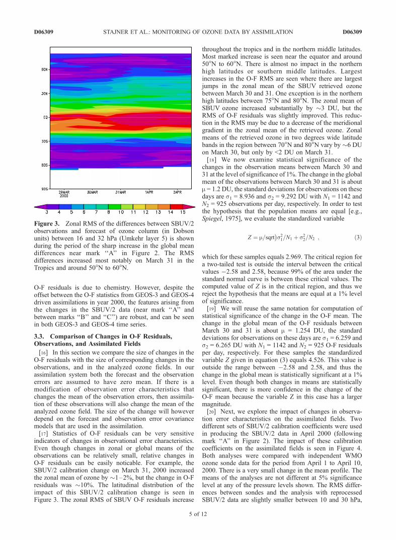
indicators of changes in observational error characteristics.Even though changes in zonal or global means of theobservations can be relatively small, relative changes inO-F residuals can be easily noticable. For example, theSBUV/2 calibration change on March 31, 2000 increasedthe zonal mean of ozone by �1–2%, but the change in O-Fresiduals was �10%. The latitudinal distribution of theimpact of this SBUV/2 calibration change is seen inFigure 3. The zonal RMS of SBUV O-F residuals increase

throughout the tropics and in the northern middle latitudes.Most marked increase is seen near the equator and around50�N to 60�N. There is almost no impact in the northernhigh latitudes or southern middle latitudes. Largestincreases in the O-F RMS are seen where there are largestjumps in the zonal mean of the SBUV retrieved ozonebetween March 30 and 31. One exception is in the northernhigh latitudes between 75�N and 80�N. The zonal mean ofSBUV ozone increased substantially by �3 DU, but theRMS of O-F residuals was slightly improved. This reduc-tion in the RMS may be due to a decrease of the meridionalgradient in the zonal mean of the retrieved ozone. Zonalmeans of the retrieved ozone in two degrees wide latitudebands in the region between 70�N and 80�N vary by �6 DUon March 30, but only by <2 DU on March 31.[18] We now examine statistical significance of the

changes in the observation means between March 30 and31 at the level of significance of 1%. The change in the globalmean of the observations between March 30 and 31 is aboutm = 1.2 DU, the standard deviations for observations on thesedays are s1 = 8.936 and s2 = 9.292 DU with N1 = 1142 andN2 = 925 observations per day, respectively. In order to testthe hypothesis that the population means are equal [e.g.,Spiegel, 1975], we evaluate the standardized variable

Z ¼ m=sqrt s21=N1 þ s22=N2

� �; ð3Þ

which for these samples equals 2.969. The critical region fora two-tailed test is outside the interval between the criticalvalues �2.58 and 2.58, because 99% of the area under thestandard normal curve is between these critical values. Thecomputed value of Z is in the critical region, and thus wereject the hypothesis that the means are equal at a 1% levelof significance.[19] We will reuse the same notation for computation of

statistical significance of the change in the O-F mean. Thechange in the global mean of the O-F residuals betweenMarch 30 and 31 is about m = 1.254 DU, the standarddeviations for observations on these days are s1 = 6.259 ands2 = 6.265 DU with N1 = 1142 and N2 = 925 O-F residualsper day, respectively. For these samples the standardizedvariable Z given in equation (3) equals 4.526. This value isoutside the range between �2.58 and 2.58, and thus thechange in the global mean is statistically significant at a 1%level. Even though both changes in means are statisticallysignificant, there is more confidence in the change of theO-F mean because the variable Z in this case has a largermagnitude.[20] Next, we explore the impact of changes in observa-

tion error characteristics on the assimilated fields. Twodifferent sets of SBUV/2 calibration coefficients were usedin producing the SBUV/2 data in April 2000 (followingmark ‘‘A’’ in Figure 2). The impact of these calibrationcoefficients on the assimilated fields is seen in Figure 4.Both analyses were compared with independent WMOozone sonde data for the period from April 1 to April 10,2000. There is a very small change in the mean profile. Themeans of the analyses are not different at 5% significancelevel at any of the pressure levels shown. The RMS differ-ences between sondes and the analysis with reprocessedSBUV/2 data are slightly smaller between 10 and 30 hPa,

Figure 3. Zonal RMS of the differences between SBUV/2observations and forecast of ozone column (in Dobsonunits) between 16 and 32 hPa (Umkehr layer 5) is shownduring the period of the sharp increase in the global meandifferences near mark ‘‘A’’ in Figure 2. The RMSdifferences increased most notably on March 31 in theTropics and around 50�N to 60�N.

D06309 STAJNER ET AL.: MONITORING OF OZONE DATA BY ASSIMILATION

5 of 12

D06309

and slightly larger near 40 hPa, than for the analysis withthe operational SBUV/2 ozone. The comparison againstHALOE data was done using �290 profiles in the Tropicsand southern middle latitudes during the first 10 days inApril 2000. This comparison also shows a very smallimpact from the change in the SBUV/2 data on the qualityof the analyzed ozone. During the same period, we com-pared the assimilated ozone against POAM data [Lumpe etal., 2002] near 65�N and found a small impact, but aslightly improved mean profile shape with the reprocessedSBUV/2 data. The RMS differences for the analysis withreprocessed SBUV/2 data are smaller between 3 and 10 hPa,and at 30 hPa, and larger elsewhere in the profile. Overall incomparisons with ozone sonde, HALOE and POAM data,we found that there was a very subtle impact on theassimilated ozone from the SBUV/2 calibration changeon March 31, 2000. The changes in the assimilated ozonefields are much less pronounced than the change in the O-Fstatistics (near mark ‘‘A’’ in Figure 2).[21] The NOAA 14 SBUV-2 instrument experienced

grating position changes during November 2000 (seechange in O-F statistics between marks ‘‘B’’ and ‘‘C’’ inFigure 2). We examine the impact of these grating positionchanges on the quality of the analyzed ozone field(Figure 5). The mean difference between assimilated ozoneand independent POAM profiles in southern high latitudesis shown for November 13 to 30 (dashed line) andfor December of 2000 (solid line). The comparison inNovember was done against 121 POAM profiles that coverbetween 70�S and 66�S. In December, 212 POAM profileswere used in the latitudes between 66�S and 63�S. Unfor-tunately, POAM data sample different latitudes at differenttimes and thus in this comparison we need to consider theunderlying geophysical variability. In order to minimize itseffects we restrict the comparison to data from consecutivemonths, and within the 7� wide latitude band. This latitude

band that is covered by POAM is also observed by SBUV/2data during November and December. A noticeably betteragreement between POAM and assimilation is seen duringDecember between 5 and 30 hPa, except at 20 hPa. The

Figure 4. Comparison of the analyses with operational SBUV/2 ozone (blue) and the reprocessedSBUV/2 ozone (red) against independent WMO ozonesonde data (black) is given for April 1–10, 2000.The means of ozonesonde profiles and collocated analyses are shown by solid lines. The RMSdifferences between sondes and each of the analyses are shown by dashed lines. Umkehr layer 5 (16 to32 hPa) is marked by the orange box. In this layer there is a small improvement in the agreement betweensondes and assimilation when reprocessed SBUV/2 data are used. This is consistent with the lower meanof O-F residuals with reprocessed SBUV/2 data following mark ‘‘A’’ in Figure 2.

Figure 5. Comparison of mean differences betweenassimilated ozone mixing ratio and independent POAMozone profiles in southern high latitudes is shown forNovember 13–30 and for December 2000. There is animprovement in the quality of assimilated ozone in themiddle stratosphere in December, which is consistent withthe decrease of the mean O-F residuals between Novemberand December seen in Figure 2.

D06309 STAJNER ET AL.: MONITORING OF OZONE DATA BY ASSIMILATION

6 of 12

D06309

means differ at 5% significance level on all pressure levelsbetween 5 and 70 hPa, except at 20 hPa. In addition, themeans differ at 1% significance level on pressure levels of3, 7, 10, 30, 40, 50, and 70 hPa. The integrated differencebetween analysis and POAM in the layer 16–32 hPadecreased in December, primarily due to a reversal of thesign of the mean difference at 30 hPa. In order to examinegeophysical significance of this change, we compare its sizewith spatial and temporal changes of the ozone mean in thisregion and period in the Upper Atmosphere ResearchSatellite extended ozone climatology (available on theWorld Wide Web at http://code916.gsfc.nasa.gov/Public/Analysis/UARS/uarp/home.html). The climatological ozonemeans at 31.6 hPa change by �0.1 ppmv between 64�S and68�S, and they change by �0.01 ppmv between Novemberand December at these latitudes. Both of these changes aresmaller than the change in the mean difference betweenanalysis and POAM at 30 hPa of �0.5 ppmv (Figure 5).The improvement in the mean difference between analysisand POAM at 30 hPa is consistent with the improvementin the mean of O-F residuals (for the layer between 16 and32 hPa) seen past mark ‘‘C’’ in Figure 2.

3.4. Concluding Remarks of Section 3

[22] The above two examples of SBUV/2 calibration andinstrument changes show that the statistics of O-F residualsfrom an assimilation system are indeed very sensitive tochanges in the observations and their error characteristics.Furthermore, these statistics are collected in near-real time,and allow a rapid feedback to the instrument team. They arealso robust over systems driven by different meteorologicaldata, and including or excluding the effects of the chemicalprocesses. In contrast to the sensitivity of O-F residuals, thechange in the assimilated ozone on March 31, 2000 wasvery subtle, and hard to detect from comparisons withindependent high quality data (sondes, POAM, andHALOE). However, during the SBUV/2 instrument gratingposition changes in November 2000, both the mean O-Fresiduals and the agreement between assimilated ozone andPOAM data were notably degraded.

4. Total Ozone Column Data

[23] In this section we examine several properties of thetotal column ozone O-F residuals: their annual variability,

their use for detection of cross-track biases of the scanningTOMS instrument, and their changes due to a switch toanother source of total column ozone data (NOAA 16SBUV/2). Finally, we study the sensitivity of the ozoneO-F residuals to changes in the meteorological assimilationsystem whose winds are used to drive the ozone assimila-tion model.

4.1. Earth Probe Total Ozone Mapping SpectrometerTotal Ozone Column Data

[24] An example of the time series of the global dailyRMS of total column ozone O-F residuals is shown inFigure 6. We focus first on the day-to-day variability seen inthis time series. In 24 hours TOMS normally provides near-global coverage of the sunlit portion of the Earth. Abruptshort-term changes in Figure 6 are typically caused by areduced coverage of total ozone observations. For example,this occurs when total ozone data file is not available ontime for the operational analysis. The only total column datathat are available are then those from the end of the last orbitthat started on the previous day because they are containedin the data file for the previous day. This happened onDecember 30, 2000 when we used only a part of one orbitgoing from southern high latitudes to the equator. In thisregion the ozone field has lower values and lower variabilitythan in the northern middle latitudes. Therefore the RMS ofO-F residuals for all observations on this day is �9.2 DU,which is well below the usual range of RMS values inDecember 2000 of �12 to 13 DU. The total ozone datawere not available for almost 5 days. When the datareturned on January 4 the O-F differences are larger (theRMS value is almost 15 DU) because of the accumulationof model errors over the 5 days for which total ozonecolumn data were not available. The RMS of O-F residualsreturns to near 12 DU within one to two days after theTOMS data become available.[25] A typical seasonal cycle is seen in Figure 6 during

the year 2000. The global RMS of total ozone O-F residualsis the lowest in January during the northern winter, whenthe northern high latitudes are in the polar night, unobservedby TOMS, and do not contribute to the global statistics.This RMS value peaks during the northern spring whenozone values increase, and the dynamical variability islarge, especially in the northern middle and high latitudeswhich are both observed by TOMS. The RMS value then

Figure 6. Time series of daily global RMS of total column ozone O-F residuals is shown. See text fordetails about marks ‘‘D’’–‘‘F’’. It shows a typical annual cycle during the year 2000. Following the mark‘‘D’’ the RMS increases due to TOMS cross-track bias and the decrease in NOAA 14 SBUV/2 coverage.After switching to the use of NOAA 16 SBUV/2 profiles (mark ‘‘E’’) and total columns (mark ‘‘F’’), theRMS decreases to near the levels seen in year 2000.

D06309 STAJNER ET AL.: MONITORING OF OZONE DATA BY ASSIMILATION

7 of 12

D06309

falls until July, and rises again until October. The increase inthe RMS of total ozone O-F residuals during northernhemisphere winter and spring (January to April) is largerin magnitude than that corresponding to the southernhemisphere winter and spring (July to October).[26] Starting in year 2000 the near-real time retrieved

total column ozone from EP TOMS began developing across-track bias that grew over time and degraded thequality of the data. According to the TOMS processingteam the bias appears to be due to a change in the opticalproperties of the front scan mirror of the instrument (newsrelease on November 15, 2001 at http://toms.gsfc.nasa.gov/news/news.html). This cross-track bias is illustrated by thescatterplot in Figure 7a. The TOMS O-F residuals at 2�S(where the geophysical variability in the total column ozonefield is relatively small, except for the zonal wave numberone) are shown by crosses for 14 orbits on January 28,2001. The O-F residuals are plotted versus the model gridpoint across the orbit, where 1 denotes the westmost and 7the eastmost grid point. The mean of O-F residuals for eachof the grid points is shown by a line, and it increases fromwest to east by 13.1 Dobson units (DU). A year earlier, onJanuary 28, 2000 the TOMS cross-track bias was smaller(Figure 7b) and the mean of O-F residuals for 14 orbits hada smaller variability of 7.6 DU. In addition, the means werecomputed for ten days (January 20 to 29) in years 2000 and2001, and the cross-track change in the means increasedfrom <3 DU in year 2000 to more than 10 DU in year 2001.

[27] A departure from the typical seasonal cycle is visiblefrom November of 2000 (just preceding mark ‘‘D’’ inFigure 6). A strong upward trend begins and culminateswith the peak in April 2001 (mark ‘‘E’’). This increase islarger than that of a typical seasonal cycle. It was due toboth the degradation of the quality of EP TOMS and a driftof the NOAA 14 orbit. The drift of the NOAA 14 orbittoward a later afternoon Equator crossing caused a decreaseof the SBUV/2 spatial coverage, an increase in the solarzenith angles of the measurements, and a consequentdegradation of the ozone products (L. Flynn, personalcommunication, 2001). In April 2001 (mark ‘‘E’’ inFigure 6) we started assimilating NOAA 16 instead ofNOAA 14 SBUV/2 profile data. The RMS of O-F residualsstarted decreasing as the ozone profiles became better con-strained by the NOAA 16 SBUV/2 observations with higherquality and better coverage than those from the NOAA 14instrument. Since May 2001 (mark ‘‘F’’ in Figure 6) totalcolumn ozone data from NOAA 16 SBUV/2 have beenassimilated instead of those from EP TOMS. This slightlyincreased the day-to-day scatter of the RMS of the O-Fresiduals, but in January 2002 they returned to valuessimilar to those of January 2000.[28] The time series of zonal RMS differences between

total column ozone observations and the forecast is shownin Figure 8. Lower values are typically found in the Tropicswhere both the total column ozone amounts and their

Figure 7. EP TOMS O-F residuals at 2� south latitude areshown by crosses as a function of the grid point across theorbit track. The westmost grid point is 1 and the eastmost is7. The mean of O-F residuals for each grid point is shownby the line. The residuals and their mean are shown onJanuary 28 of the year 2001 in Figure 7a and year 2000 inFigure 7b.

Figure 8. Time series of the zonal RMS differencebetween total column observations and the forecast fromthe near-real time ozone assimilation system (in Dobsonunits) is shown. A typical distribution is seen in year 2000:the lowest RMS differences are within the ‘‘ozone hole’’region (in the high southern latitudes in September andOctober), relatively low differences are in the Tropics, andthe highest differences are in middle to high latitudes duringspringtime in both hemispheres. A buildup in the RMSdifferences is seen from about December 2000 to May 2001.The abrupt reduction in the latitudinal coverage of the totalcolumn ozone data in May 2001 occurs because the sourceof total column ozone data was changed from EP TOMS toNOAA 16 SBUV/2. White areas indicate that data were notavailable for a specific time and latitude, e.g., within thepolar night, or when a data file is missing for a day.

D06309 STAJNER ET AL.: MONITORING OF OZONE DATA BY ASSIMILATION

8 of 12

D06309

spatio-temporal variability are lower than in extratropics.The RMS differences and the ozone amounts are lower onlyinside the Antarctic ‘‘ozone hole’’ which is seen in thesouthern high latitudes around October. The RMS differ-ences are typically higher in middle latitudes, especially inwinter and spring when total ozone amounts as well as theirdynamical variability increase. Note that most of the build-up in the global RMS of total ozone O-F residuals (seenbetween marks ‘‘D’’ and ‘‘E’’ in Figure 6) begins innorthern middle latitudes in December 2000, extends tonorthern high latitudes in February 2001, and anotherbuildup is seen in southern high latitudes around April2001.

4.2. NOAA 16 SBUV//2 Total Ozone Column Data

[29] During May 2001, when the ozone assimilationsystem started using NOAA 16 SBUV/2 total column ozonedata instead of EP TOMS data, an abrupt change occurs inspatial coverage (Figure 8): the latitudinal coveragedecreases by �5� in the northern hemisphere, and by�15� in the southern hemisphere. After several days ofthe initial adjustment of the system to the total column datafrom NOAA 16 SBUV/2, the RMS differences in thenorthern middle and high latitudes decrease. The RMS inthe southern middle latitudes increases as expected from theprevious annual cycle. The RMS values in the southernTropics are just slightly higher than those seen in the year2000 when the TOMS data were assimilated. However, theRMS values in the northern tropics between May andDecember of year 2001 are higher than during previousperiods. The SBUV/2 instrument provides measurements atnadir points only, for �14 orbits per day. In contrast, EPTOMS is a scanning instrument that provides almostcomplete coverage of the Tropics every day. About10,000 total column observations were used daily fromEP TOMS, compared to �900 observations from NOAA16 SBUV/2. The observation error standard deviation usedfor SBUV total ozone is 3% of the observed value. TheSBUV footprint is comparable to the model grid cell, so therepresentativeness error is not modeled. For TOMS totalozone the observation error variance is the sum of thesquares of two terms: the measurement and retrieval errorstandard deviation, which is 1.5% of the observed value,and the representativeness error standard deviation, whichtypically ranges between 3 and 7 DU [Stajner et al., 2001].With sparser total column ozone data from SBUV/2, andoften higher observation errors, the forecast relies moreheavily on the model, and the forecast errors explain a largerportion of the O-F residuals.

4.3. Changes in the Meteorological System

[30] The zonal RMS of O-F residuals (in Figure 8,especially in the Tropics) and the zonal mean of O-Fresiduals (not shown) decrease in December 2001 followingseveral simultaneous changes in the meteorological GEOS-3assimilation system. One of the changes in the meteorolog-ical system was the use of in-house TOVS retrievals,including moisture data, instead of NESDIS TOVS retriev-als. Another change was made to the radiation package of thegeneral circulation model, to parameterize the effects of tracegasses. Assimilation of total precipitable water and the land-surface emissivities were also modified. The wind analysis

increments were constrained so that the vertically averagedvelocity potential vanishes. Forecast error variances werechanged to be uniform on each level. However, all thesechanges to the meteorological system were introducedsimultaneously, and it is not clear which ones had the largesteffect on the ozone transport.

4.4. Discussion

[31] We found that the total column ozone O-F residualsare sensitive to instrument cross-track biases. The size ofO-F residuals changes with a switch in the instrumentwhose total column data are used. The O-F residuals arealso sensitive to changes in the meteorological systemused to produce winds that drive ozone transport in theozone assimilation system. Thus the ozone O-F residualscan be used for indirect evaluation of the transportproperties of assimilated winds, especially in the strato-sphere, which contains the most of the ozone column.

5. NOAA 16 SBUV//2 Ozone Profiles

[32] The NOAA 16 SBUV/2 instrument became opera-tional in early 2001. This first year of operations providesan interesting period for evaluating changes in the errorcharacteristics of the retrieved ozone data. During thisperiod the instrument characteristics become better knownand frequently some modifications are made to instrumentcalibration and to the retrieval algorithm. We will show howthese changes are detected in assimilation and how theyaffect the assimilated ozone field.[33] Daily monitoring of the NOAA 16 SBUV/2 O-F

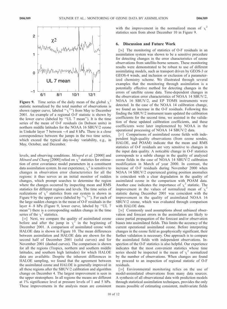
residual regional statistics was implemented in May 2001.In the next example we focus on the SBUVobservations inthe Umkehr layer 7, between �4 and 8 hPa. There is �20–25 DU of ozone in this layer and the spatial standarddeviation is �3–4 DU. The mean of the O-F residuals inthe northern middle latitudes for this layer is shown inFigure 9 (lower curve, labeled by ‘‘UL 7 mean’’). Largerthan typical variability can be seen in May, around October 9and 13, and December 6. The change on October 13 wascaused by the unintended use of NOAA 14 instead ofNOAA 16 SBUV/2 data in the assimilation, and the biasbetween these two SBUV/2 data sets. Each of the otherthree jumps in the O-F statistics coincides with a change ineither instrument calibration or in the operational retrievalalgorithm used to produce NOAA 16 SBUVozone data: thephotomultiplier tube temperature correction was changed inthe retrieval algorithm in May, the calibration was changedto use automatic inter-range ratio update using on-orbit datainstead of extrapolated time dependent table on October 9,and finally in December the calibration started using newtime dependent albedo correction factors and the retrievalalgorithm for pressure mixing of ozone estimates for dif-ferent wavelength pairs was modified (S. Kondragunta,personal communication, 2001).[34] One convenient statistic for monitoring of the changes

in the O-F residuals is z/p (for z from equation (2)), themean of c2 statistics normalized by the number of observa-tions. Recall that under the ideal conditions its value shouldbe one. This statistic accounts for all the O-F residualsaccording to their error covariances. It provides one globalnumber representing all residuals from different regions,

D06309 STAJNER ET AL.: MONITORING OF OZONE DATA BY ASSIMILATION

9 of 12

D06309

levels, and observing conditions. Menard et al. [2000] andMenard and Chang [2000] relied on c2 statistics for estima-tion of error covariance model parameters in a constituentdata assimilation system. In our experience, c2 is sensitive tochanges in observation error characteristics for all theregions: it thus serves as an initial monitor of suddenchanges, which prompt searches to determine the regionwhere the changes occurred by inspecting mean and RMSstatistics for different regions and levels. The time series ofrealizations of c2 statistics from our system is shown inFigure 9 by the upper curve (labeled by ‘‘c2’’). For each ofthe large sudden changes in the mean of O-F residuals in thelayer 4–8 hPa (Figure 9, lower curve, labeled by ‘‘UL 7mean’’) there is a corresponding sudden change in the timeseries of the c2 statistics.[35] Next, we compare the quality of assimilated ozone

before and after the jump in c2 in the beginning ofDecember 2001. A comparison of assimilated ozone withHALOE data is shown in Figure 10. The mean differencesbetween assimilation and HALOE data are shown for thesecond half of December 2001 (solid curves) and forNovember 2001 (dashed curves). The comparison is shownfor all the regions (Tropics, northern and southern middlelatitudes, and southern high latitudes) for which HALOEdata are available. Despite the inherent differences inHALOE sampling, we found that the agreement betweenthe assimilated ozone and HALOE is generally improved inall these regions after the SBUV/2 calibration and algorithmchange on December 4. The largest improvement is seen inthe upper stratosphere. In all regions the means are differentat 1% significance level at pressure levels of 1 and 5 hPa.These improvements in the analysis mean are consistent

with the improvement in the normalized mean of c2

statistics seen from about December 10 in Figure 9.

6. Discussion and Future Work

[36] The monitoring of statistics of O-F residuals in anassimilation system was shown to be a sensitive procedurefor detecting changes in the error characteristics of ozoneobservations from satellite-borne sensors. These monitoringresults were demonstrated to be robust to use of differentassimilating models, such as transport driven by GEOS-3 orGEOS-4 winds, and inclusion or exclusion of a parameter-ized chemistry scheme. We illustrated through severalexamples that the monitoring through assimilation is apotentially effective method for detecting changes in theerrors of satellite ozone data. Time-dependent changes inthe observation error characteristics of NOAA 14 SBUV/2,NOAA 16 SBUV/2, and EP TOMS instruments weredetected. In the case of the NOAA 14 calibration change,we found an increase in the O-F residuals. Following thisfinding the SBUV/2 instrument team updated the calibrationcoefficients for the second time, we assisted in the valida-tion of these updated calibration coefficients, and thesecoefficients were later implemented by NOAA in theoperational processing of NOAA 14 SBUV/2 data.[37] Comparisons of assimilated ozone fields with inde-

pendent high-quality observations (from ozone sondes,HALOE, and POAM) indicate that the mean and RMSstatistics of O-F residuals are very sensitive to changes inthe input data quality. A noticable change in O-F statisticscorresponds to a subtle change in the quality of analyzedozone fields in the case of NOAA 14 SBUV/2 calibrationmodification in March of year 2000. In contrast, theincrease of O-F residuals during November 2000 whenNOAA 14 SBUV/2 experienced grating position anomaliesis coincident with a clear degradation in the quality ofassimilated ozone in the comparison with POAM data.Another case indicates the importance of c2 statistic. Theimprovement in the values of normalized mean of c2

statistic during December 2001 was coincident with theimprovement in the quality of assimilated NOAA 16SBUV/2 ozone, which was evaluated through comparisonwith HALOE data.[38] Commonly used assumptions about unbiased obser-

vation and forecast errors in the assimilation are likely tocause partial propagation of the forecast and/or observationbiases into assimilated fields. This limits the accuracy of thecurrent operational assimilated ozone. Before interpretingchanges in the ozone field as geophysically significant, theirfurther validation is necessary. One approach is to comparethe assimilated fields with independent observations. In-spection of the O-F statistics is also helpful. Our experienceindicates that the most convenient statistics whose timeseries should be inspected is the mean of c2 normalizedby the number of observations. When changes are foundwe proceed to an inspection of regional statistic of O-Fresiduals.[39] Environmental monitoring relies on the use of

model-assimilated observations from many data sources.A synthesis of all observational data with prediction modelsthrough statistical assimilation techniques, provides the onlymeans possible of estimating consistent, multivariate fields

Figure 9. Time series of the daily mean of the global c2

statistic normalized by the total number of observations isshown (upper curve, labeled ‘‘c2’’) from May to December2001. An example of a regional O-F statistic is shown bythe lower curve (labeled by ‘‘UL 7 mean’’). It is the timeseries of the mean of O-F residuals (in Dobson units) innorthern middle latitudes for the NOAA 16 SBUV/2 ozonein Umkehr layer 7 between �4 and 8 hPa. There is a closecorrespondence between the jumps in the two time series,which exceed the typical day-to-day variability, e.g., inMay, October, and December.

D06309 STAJNER ET AL.: MONITORING OF OZONE DATA BY ASSIMILATION

10 of 12

D06309

of environmental parameters [National Research Council,1991]. This synthesis is typically done in two ways:operationally in near-real time using different, ever improv-ing models, and in the ‘‘reanalysis’’ framework where afixed state-of-the-art model and a fixed statistical assimila-tion technique are used over an extended historical period[Schubert et al., 1993; Kalnay et al., 1996; Gibson et al.,1997; Simmons and Gibson, 2000]. Both types of synthesisare affected by inevitable discontinuities between instru-ments or even the types of environmental observations thatare available for usage.[40] The validation statistics presented in this study

contain some results applicable to reanalyses, while othersare relevant only to ‘‘real-time’’ operational monitoring.Examples of the latter are changes in ozone forecast modelbrought about by the meteorological analyses (changes inGEOS-3 in December 2001) and by the combination ofintroducing a parameterized ozone chemistry model at thesame time as changing from GEOS-3 to GEOS-4 analyses(the ‘‘reanalysis’’ shown in Figure 2). The most importantissues for reanalysis pertain to the unavoidable changes ininstruments and to the time dependence of the data qualityfrom any one instrument. Two important effects, the degra-dation of EP-TOMS data quality and the effective loss ofNOAA 14 SBUV/2 data caused by the orbital drift, hadmarked impacts on the quality of the resultant ozoneanalyses, clearly characterized by the long-term behavior

of the monitoring statistics. For reanalysis purposes, theseeffects must be considered.[41] In a near-real time system, the re-calibration of

SBUV/2 retrievals had an impact on analysis quality, aneffect not immediately obvious from the analyses, butclearly evident in the O-F residuals. Effects such as these,which can also be detected by careful monitoring of theretrieved data without assimilation, are crucial to the successand realism of analyses. The fundamental point about thatanalysis is not that assimilation can detect changes in theretrieval algorithms (these should be known anyway): it isthat assimilation can isolate the impacts of such changesand, in the context of an end-to-end environmental moni-toring system, can provide quantitative measures of theseimpacts and offer guidance into producing more appropriatechanges that lead to a smaller shock to the system. Theunderlying message of this work is that careful use of themonitoring statistics, alongside the assimilated products,can yield a beneficial insight into the quality of the dataand the suitability of any long-term analyses for inferringglobal change through quantitative, robust measures of themodel-data uncertainty.[42] Several instruments that measure ozone are included

on the recent and planned satellites: Earth ObservingSystem (EOS) Aqua, EOS Aura, and Environmental Satel-lite (Envisat). We have already applied the monitoringthrough assimilation for ozone observations from Envisat,

Figure 10. Regional mean differences between analyzed ozone and HALOE data before (dashed) andafter (solid) the calibration and algorithm change in NOAA 16 SBUV/2 retrievals on December 4, 2001are shown. Following the change in the retrievals there is generally an improvement in the quality of theassimilated ozone profile, especially at pressures <10 hPa.

D06309 STAJNER ET AL.: MONITORING OF OZONE DATA BY ASSIMILATION

11 of 12

D06309

from the AIRS instrument on EOS Aqua, and from theMicrowave Limb Sounder onboard NASA’s Upper Atmo-sphere Research Satellite. We plan to extend the monitoringthrough assimilation to retrieved ozone data from instru-ments on EOS Aura.

[43] Acknowledgments. We are thankful for discussions and collab-oration with scientists from SBUV/2 and EP TOMS instrument teams, inparticular M. Deland, D. McNamara, S. Kondragunta, L. Flynn, P. K.Bhartia, and R. McPeters. We are grateful to the operations group atNASA’s Global Modeling and Assimilation Office, which maintains andruns the operational ozone system, and in particular to R. Lucchesi whohelped implement modifications to the operational system. We are thankfulto two anonymous reviewers whose suggestions helped improve thismanuscript. This work was supported by NASA HQ, partly through OzoneMonitoring Instrument science team grant 229-07-27 and partly by NASA’sAtmospheric Chemistry and Modeling Program grant 622-55-61.

ReferencesAtlas, R., S. C. Bloom, R. N. Hoffman, E. Brin, J. Ardizzone, J. Terry,D. Bungato, and J. C. Jusem (1999), Geophysical validation of NSCATwinds using atmospheric data and analyses, J. Geophys. Res., 104,11,405–11,424.

Aumann, H. H., et al. (2003), AIRS/AMSU/HSB on the Aqua mission:Design, science objectives, data products, and processing systems, IEEETrans. Geosci. Remote Sens., 41, 253–264.

Austin, J. (1992), Toward the four dimensional assimilation of stratosphericconstituents, J. Geophys. Res., 97, 2569–2588.

Bhartia, P. K., R. D. McPeters, C. L. Mateer, L. E. Flynn, and C. Wellemeyer(1996), Algorithm for the estimation of vertical ozone profile from thebackscattered ultraviolet (BUV) technique, J. Geophys. Res., 101,18,793–18,806.

Bruhl, C., et al. (1996), HALOE Ozone Channel Validation, J. Geophys.Res., 101, 10,217–10,240.

Daley, R. (1991), Atmospheric Data Analysis, Cambridge Univ. Press, NewYork.

Dethof, A., and E. Holm (2002), Ozone in ERA-40: 1991–1996, ECMWFTech. Memo., 377, 31 pp.

Elbern, H., and H. Schmidt (2001), Ozone episode analysis by four-dimen-sional variational chemistry data assimilation, J. Geophys. Res., 106,3569–3590.

Eskes, H. J., A. J. M. Piters, P. F. Levelt, M. A. F. Allaart, and H. M. Kelder(1999), Variational assimilation of GOME total-column ozone satellitedata in a 2 D latitude-longitude tracer-transport model, J. Atmos. Sci., 56,3560–3572.

Eskes, H. J., P. F. J. van Velthoven, P. J. M. Valks, and H. M. Kelder (2003),Assimilation of GOME total ozone satellite observations in a three-di-mensional tracer transport model, Q. J. R. Meteorol. Soc., 129, 1663–1681.

Fetzer, E., et al. (2003), AIRS/AMSU/HSB validation, IEEE Trans. Geosci.Remote Sens., 41, 418–431.

Fisher, M., and D. J. Lary (1995), Lagrangian four-dimensional variationaldata assimilation of chemical species, Q. J. R. Meteorol. Soc., 131,1681–1704.

Fleming, E. L., C. H. Jackman, D. B. Considine, and R. S. Stolarski (2001),Sensitivity of tracers and a stratospheric aircraft perturbation to two-di-mensional model transport variations, J. Geophys. Res., 106, 14,245–14,263.

Froidevaux, L., et al. (1996), Validation of UARS Microwave Limb Soun-der ozone measurements, J. Geophys. Res., 101, 10,017–10,060.

Gibson, J. K., P. Kallberg, S. Uppala, A. Nomura, A. Hernandez, andE. Serrano (1997), ERA Description. ECMWF Reanal. Final Rep. Ser.,1, 71 pp.

Gille, J. C., et al. (1996), Accuracy and precision of Cryogenic Limb ArrayEtalon Spectrometer (CLAES) temperature retrievals, J. Geophys. Res.,101, 9583–9602.

Hollingsworth, A., D. B. Shaw, P. Lonnberg, L. Illari, K. Arpe, and A. J.Simmons (1986), Monitoring of observation and analysis quality by adata assimilation system, Mon. Wea. Rev., 114, 861–879.

Hollingsworth, A., P. Viterbo, and A. J. Simmons (2003), The relevanceof numerical weather prediction for forecasting natural hazards and formonitoring the global environment, in A Half Century of Progressin Meteorology: A Tribute to Richard J. Reed, edited by R. H.

Johnson and R. A. Houze Jr., pp. 109–129, Am. Meteorol. Soc.,Boston, Mass.

Kalnay, E., et al. (1996), The NCEP/NCAR 40-year reanalysis project, Bull.Am. Meteorol. Soc., 77, 437–471.

Khattatov, B. V., J.-F. Lamarque, L. V. Lyjak, R. Menard, P. F. Levelt, X. X.Tie, G. P. Brasseur, and J. C. Gille (2000), Assimilation of satellite ob-servations of long-lived chemical species in global chemistry-transportmodels, J. Geophys. Res., 105, 29,135–29,144.

Langematz, U. (2000), An estimate of the impact of observed ozone losseson stratospheric temperature, Geophys. Res. Lett., 27, 2077–2080.

Levelt, P. F., B. V. Khattatov, J. C. Gille, G. P. Brasseur, X. X. Tie, and J. W.Waters (1998), Assimilation of MLS ozone measurements in the globalthree-dimensional chemistry transport model ROSE, Geophys. Res. Lett.,25, 4493–4496.

Lin, S.-J., and R. B. Rood (1996), Multidimensionsl flux-form semi-langrangian transport schemes, Mon, Wea. Rev., 124, 2046–2070.

Long, C. S., A. J. Miller, H. T. Lee, J. D. Wild, R. C. Przywarty, andD. Hufford (1996), Ultraviolet index forecasts issued by the NationalWeather Service, Bull. Am. Meteorol. Soc., 77, 729–748.

Lumpe, J. D., R. M. Bevilacqua, K. W. Hoppel, and C. E. Randall (2002),POAM III retrieval algorithm and error analysis, J. Geophys. Res.,107(D21), 4575, doi:10.1029/2002JD002137.

McPeters, R. D., et al. (1998), Earth Probe Total Ozone Mapping Spectro-meter (TOMS) Data Products User’s Guide, NASA Tech. Publ. 1998-206895, NASA, Washington, D. C.

Menard, R., and L.-P. Chang (2000), Assimilation of stratospheric chemicaltracer observations using a Kalman filter, Part II: c2–validated resultsand analysis of variance and correlation dynamics, Mon. Wea. Rev., 128,2672–2686.

Menard, R., S. E. Cohn, L.-P. Chang, and P. M. Lyster (2000), Assimilationof stratospheric chemical tracer observations using a Kalman filter. Part I:Formulation, Mon. Wea. Rev., 128, 2654–2671.

National Research Council (1991), Four-Dimensional Model Assimilationof Data: A Strategy for the Earth System Sciences, Natl. Acad. Press,Washington, D. C.

Piters, A. J. M., P. F. Levelt, M. A. F. Allaart, and H. M. Kelder (1999),Validation of GOME total ozone column with the Assimilation ModelKNMI, Remote Sensing: Earth, Ocean and Atmosphere, 22, 1501–1504.

Remsberg, E., et al. (2002), An assessment of the quality of HalogenOccultation Experiment temperature profiles in themesosphere based oncomparisons with Rayleigh backscatter lidar and inflatable falling spheremeasurements, J. Geophys. Res., 107(D20), 4447, doi:10.1029/2001JD001521.

Riishøjgaard, L. P., I. Stajner, and G.-P. Lou (2000), The GEOS ozone dataassimilation system, Adv. Space Res., 25, 1063–1072.

Rodgers, C. D., and B. J. Connor (2003), Intercomparison of remote sound-ing instruments, J. Geophys. Res., 108(D3), 4116, doi:10.1029/2002JD002299.

Schubert, S. D., R. B. Rood, and J. Pfaentner (1993), An assimilated datasetfor Earth science applications, Bull. Am. Meteorol. Soc., 77, 437–471.

Simmons, A. J., and J. K. Gibson (2000), The ERA-40 project plan, Era-40Proj. Rep. Ser., 1, 63 pp.

Smith, W. L., H. M. Woolf, C. M. Hayden, D. Q. Wark, and L. M. McMillin(1979), The TIROS-N operational vertical sounder, Bull. Am. Meteorol.Soc., 60, 1177–1187.

Spiegel, M. R. (1975), Schaum’s Outline of Theory and Problems of Prob-ability and Statistics, McGraw-Hill, New York.

Stajner, I., L. P. Riishøjgaard, and R. B. Rood (2001), The GEOS ozone dataassimilation system: Specification of error statistics, Q. J. R. Meteorol.Soc., 127, 1069–1094.

Stoffelen, A. (1999), A simple method for calibration of a scatterometerover the ocean, J. Atmos. Ocean Tech., 16, 275–282.

Struthers, H., R. Brugge, W. A. Lahoz, A. O’Neill, and R. Swinbank(2002), Assimilation of ozone profiles and total column measurementsinto a global general circulation model, J. Geophys. Res., 107, 4438,doi:10.1029/2001JD000957.

Uppala, S. (1997), Observing system performance in ERA, ECMWFReanal. Proj. Rep. Ser., 3, 261 pp.

�����������������������S. Pawson, R. Rood, I. Stajner, and N. Winslow, Global Modeling and

Assimilation Office, Code 900.3, NASA Goddard Space Flight Center,Greenbelt, MD 20771, USA. (spawson@gmao.gsfc.nasa.gov; rrood@gmao.gsfc.nasa.gov; istajner@gmao.gsfc.nasa.gov; nwinslow@gmao.gsfc.nasa.gov)

D06309 STAJNER ET AL.: MONITORING OF OZONE DATA BY ASSIMILATION

12 of 12

D06309