Monotonicity in Asymmetric First-Price Auctions with Affiliation David McAdams * Abstract I study monotonicity of equilibrium strategies in first-price auc- tions with asymmetric bidders, risk-aversion, affiliated types, and in- terdependent values. I prove that every mixed-strategy equilibrium is outcome equivalent to a monotone pure strategy equilibrium un- der the “priority rule” for breaking ties. This provides a missing link to establish uniqueness in Milgrom and Weber (1982)’s “general sym- metric model”. Non-monotone equilibria can exist under the “coin-flip rule” but they are distinguishable: all non-monotone equilibria have positive probability of ties whereas all monotone equilibria have zero probability of ties. This provides a justification for the standard em- pirical practice of restricting attention to monotone strategies. * E-mail: [email protected]. Post: MIT Sloan School of Management, E52-448, 50 Memorial Drive, Cambridge, MA 02142. I thank Eddie Dekel and Phil Reny for providing helpful comments at an early stage of this work and seminar participants at CalTech, Harvard/MIT, Northwestern, Princeton, and UC Berkeley for comments on a more recent version of the paper. This research has been supported by National Science Foundation grant #SES-0241468. 1
Transcript
Monotonicity in Asymmetric First-Price
Auctions with Affiliation
David McAdams∗
Abstract
I study monotonicity of equilibrium strategies in first-price auc-
tions with asymmetric bidders, risk-aversion, affiliated types, and in-
terdependent values. I prove that every mixed-strategy equilibrium
is outcome equivalent to a monotone pure strategy equilibrium un-
der the “priority rule” for breaking ties. This provides a missing link
to establish uniqueness in Milgrom and Weber (1982)’s “general sym-
metric model”. Non-monotone equilibria can exist under the “coin-flip
rule” but they are distinguishable: all non-monotone equilibria have
positive probability of ties whereas all monotone equilibria have zero
probability of ties. This provides a justification for the standard em-
pirical practice of restricting attention to monotone strategies.
∗E-mail: [email protected]. Post: MIT Sloan School of Management, E52-448, 50Memorial Drive, Cambridge, MA 02142. I thank Eddie Dekel and Phil Reny for providinghelpful comments at an early stage of this work and seminar participants at CalTech,Harvard/MIT, Northwestern, Princeton, and UC Berkeley for comments on a more recentversion of the paper. This research has been supported by National Science Foundationgrant #SES-0241468.
1
1 Introduction
A large and growing literature, both empirical and experimental, studies
first-price auctions with the goal of testing whether observed behavior is con-
sistent with equilibrium and/or of estimating the distribution of unobserv-
ables taking equilibrium behavior as given.1 In symmetric settings, these pa-
pers focus on the symmetric monotone pure strategy equilibrium (“MPSE”)
demonstrated by Milgrom and Weber (1982). In asymmetric settings, they
focus on MPSE guaranteed to exist by Reny and Zamir (2004). In either
case, the possibility of non-monotone (including mixed strategy) equilibria
is effectively ignored. But if such equilibria exist, then the conclusions of
this literature would be jeopardized since they might be based on selecting
the “wrong equilibrium.” This paper raises an unnoticed problem with this
literature and then proposes a solution.
The problem is that first-price auctions can possess non-monotone equi-
libria. In fact, I provide an example in which a non-monotone equilibrium
Pareto dominates all monotone equilibria, i.e. all bidders and the auction-
eer are better off in a non-monotone equilibrium than in every monotone
equilibrium. No one has ever observed non-monotone bidding in first-price
auctions in the field or in the laboratory, but this might simply be because
the standard tools used to study auction data implicitly assume monotonic-
ity. (When other bidders adopt monotone strategies, each bidder’s first-order
condition at bid-level b can be expressed simply in terms of others’ types who
bid b. The standard approach in the empirical literature is to use such first-
order conditions for identification purposes, but this is not valid if others
adopt non-monotone strategies.)
My solution to this problem is three-fold. First, I show that the existence
of non-monotone equilibria hinges crucially on the combination of affiliated
1Hendricks, Pinkse, and Porter (2003) provide an overview of recent empirical work.For a survey of experimental work see Kagel and Levin (2002).
2
types and interdependent values. If bidders have (i) affiliated private values
or (ii) interdependent values but independent types, then all equilibria must
be MPSE. (See the discussion in Section 4.) Second, the existence of non-
monotone equilibria hinges crucially on the details of the tie-breaking rule.
Consider an alternative “priority rule” under which each bidder is assigned
a priority before the bidding takes place and, in the event of a tie, the bid-
der with the highest priority wins. Given the priority rule, all equilibria are
monotone. (See Theorem 2.) Third, when they do exist under the standard
coin-flip rule, non-monotone equilibria are distinguishable from monotone
equilibria. In particular, all non-monotone equilibria have a positive prob-
ability of ties whereas all monotone equilibria have zero probability of ties.
(See Theorem 1.) In fact, as discussed in Section 4, three or more bidders
must submit the same bid with positive probability in any non-monotone
equilibrium. Thus, one may conclude that non-monotone equilibrium is not
being played if such three-way ties do not occur.
Proving that all equilibria are monotone has the extra benefit of imply-
ing equilibrium uniqueness in those special cases in which others have proven
uniqueness of MPSE. In particular, until now it has remained an open ques-
tion whether there is a unique equilibrium in Milgrom and Weber (1982)’s
classic “general symmetric model”. Milgrom and Weber (1982)’s argument
implies that this equilibrium is the unique symmetric MPSE and McAdams
(2004) proves that there are no asymmetric MPSE, but the hardest problem
is ruling out non-monotone equilibria. Thus, this paper provides the missing
link for proving uniqueness in one of the most widely used first-price auction
models.
The most closely related paper is Rodriguez (2000). He proves in the case
of two bidders that all equilibria in the first-price auction must be monotone
“within the support of winning bids”. My result is stronger in that (i) there
are n ≥ 2 bidders and (ii) all equilibria must be monotone over the range of all
bids, including losing bids. (Result (ii) eliminates the possibility that there
3
might be some non-monotone equilibrium that “looks like” it has monotone
strategies when we restrict attention to the winning bids but which is not
outcome-equivalent to any monotone equilibrium. See Lemma 2.) Like Ro-
driguez, I allow for asymmetric bidders, risk-aversion, affiliated types, and/or
interdependent values.
The rest of the paper is organized as follows. Section 2 lays out the
model. Section 3 sketches the proof of the main result. Section 4 provides
an example of a non-monotone equilibrium and related discussion. Section
5 concludes the paper with some remarks and directions for future work.
Since the analysis is quite technical, most formal proofs are relegated to an
Appendix.
2 Model
There are n asymmetric bidders and one object. The assumptions on infor-
mation and payoffs are identical to those of Reny and Zamir (2004).
Information: Bidder types are one-dimensional with joint density f(t) on
the unit cube [0, 1]n. For each subset I ⊂ {1, ..., n}, the conditional joint
density will be denoted f(tI |t−I) where t ≡ (t1, ..., tn), tI ≡ (ti : i ∈ I), and
−I ≡ {1, ..., n}\I. (Bold notation will be used throughout the paper to
refer to vectors of types, bids, and strategies.) Each bidder also receives a
“randomization variable” τi, where τ = (τ1, ..., τn) are i.i.d. uniform on [0, 1]
and independent of types.
(A1) f(·) is measurable and positive on [0, 1]n
(A2) Bidder types t are affiliated, i.e. f(t′ ∨ t)f(t′ ∧ t) ≥ f(t′)f(t) for all
type profiles t′, t, where ∨ and ∧ denote component-wise maximum
and minimum, respectively
Affiliation is a powerful form of positive correlation that allows us to establish
4
that certain conditional expectations are non-decreasing. (See Milgrom and
Weber (1982) for more detailed discussion.)
Payoffs: Bidder i’s utility upon losing is zero and upon winning with bid b
has form ui(t; b). I make the following assumptions on utility: for all i,
(A3) ui measurable and continuous in b,
(A4) ui strictly increasing in ti, non-decreasing in tj for all j 6= i, and strictly
decreasing in b,
(A5) ui(t; b′)− ui(t; b) non-decreasing in t for all b′ > b, and
(A6) u(1; ph) < 0 for some bid level ph < ∞.
Bids: After learning ti and τi, each bidder submits bid bi(ti; τi) ∈ OUT ∪ P .
Under a “continuum price grid”, P = [0,∞). Otherwise under a “general
price grid”, P is an arbitrary closed subset of the real line, e.g. finite. Bid-
ding is voluntary: a bidder who chooses not to participate “bids” OUT .
When bidders do not randomize, I will use bi(ti) to denote type ti’s bid.
Also, to avoid tedious technical complications, I will assume that each bid
function bi(ti; τi) is measurable in both ti, τi and that the correspondence
{b : b = bi(ti; τi) for some τi} is piecewise continuous in ti.
Outcomes: If all bidders bid OUT , then the auction is cancelled. Otherwise
for a given profile of bids b, the winner is a bidder from the set of highest
bidders, I(b) ≡ arg max1≤i≤n bi, and pays its bid. I will consider two sorts of
tie-breaking rules:
Definition 1 (Tie-breaking by coin-flip): Each member of I(b)
wins with probability 1/#(I(b)).
Definition 2 (Tie-breaking by priority): The winner is whomever
has the highest priority among the tying bidders. That is, arg maxi∈I(b) ρ(i)
5
wins, where ρ is a permutation of {1, ..., n} (“priority ranking”) that is known
before the bidding takes place.
Ultimately, both rules may be thought of as ranking the bidders and awarding
the object to the member of I(b) with the highest rank. The difference is
that under the coin-flip rule bidders are ranked after they submit their bids
whereas in the priority rule they are ranked before they bid.
Definition 3 (Serious bid): b > OUT is a serious bid for bidder i
given others’ strategies b−i(·; ·) if it is high enough to win outright (win with-
out tying) with positive probability, i.e. Prt−i,τ−i(b > maxj 6=i bj(tj; τj)) > 0.
Definition 4 (Outcome-Equivalent (“OE”)): Two strategy pro-
files b′(·; ·) and b(·; ·) are outcome-equivalent if the high bid and the set of
bidders submitting the high bid are the same with probability one:
Pr(max
ib′i(ti; τi) = max
ibi(ti; τi)
)= 1 and
Pr(arg max
ib′i(ti; τi) = arg max
ibi(ti; τi)
)= 1
Equivalently, b′(·; ·) and b(·; ·) are OE iff b′i(ti; τi) = bi(ti; τi) for all bidders i
and a full measure set of those (ti; τi) for which either b′i(ti; τi) or bi(ti; τi) is
a serious bid.
Definition 5 (Equilibrium, Monotone): The profile b∗(·; ·) is a
mixed strategy equilibrium (“MSE”) when, for each bidder i and all pairs
(ti, τi), b∗i (ti, τi) is a best response, i.e. maximizes bidder i’s expected payoff
conditional on ti and others’ strategies. The MSE b∗(·; ·) is monotone iff
inf bi(t′i) ≥ sup bi(ti) for all t′i > ti. A monotone pure strategy equilibrium
(“MPSE”) is a monotone MSE in which b∗i (ti; τ′i) = b∗i (ti; τi) ≡ b∗i (ti) for all
ti, τ′, τ .
Notes: (a) Any monotone MSE involves mixing by at most countably many
types and hence is outcome-equivalent to a MPSE. Thus, this paper’s inquiry
is ultimately directed at whether equilibria are monotone or non-monotone,
6
not at whether they are pure or mixed. (b) The full-support assumption
on the joint distribution of bidders’ types is important to the results since
extreme positive correlation of bidders’ types can lead to existence of non-
monotone equilibria. For a simple example, suppose that there are three
bidders with private values that are always equal and distributed over [0, 1].
In addition to the MPSE in which bi(vi) = vi for each bidder i, mixed-strategy
equilibria exist that are not outcome-equivalent to any MPSE. In one such
equilibrium, bi(vi) = vi for i = 1, 2 but bidder 3 adopts a mixed strategy:
b3(vi; τi) = 2τivi when τi ∈ [0, 1/2] and b3(vi; τi) = vi if τi ∈ [1/2, 1]. No
outcome-equivalent monotone strategy profile exists to this mixed strategy
equilibrium, so certainly no outcome-equivalent MPSE exists.
3 Monotone Equilibria
Reny and Zamir (2004) prove that monotone pure strategy equilibrium (“MPSE”)
exists. The question addressed here is whether any mixed strategy equilibria
(“MSE”) exist that are not outcome-equivalent to MPSE.
Definition 6 (Zero probability of ties): A mixed-strategy equi-
librium b∗(·; ·) has zero probability of ties if Prt,τ(b∗i (ti, τi) = b∗j(tj, τj)
)= 0
for all pairs of bidders i, j.
Theorem 1: Given tie-breaking by coin-flip and a continuum price grid,
every MSE in the first-price auction with zero probability of ties is outcome-
equivalent to some MPSE.
Theorem 2: Given tie-breaking by priority and a general price grid, ev-
ery MSE in the first-price auction is outcome-equivalent to some MPSE.
3.1 Proof sketch for Theorems 1,2
For a relatively simple illustration of what drives equilibria to be monotone,
consider an equilibrium with n bidders and three simplifying properties: for
7
t1 or t2
b2
��
��
��
��
��
��
��
��
��
���
b1(·)
t̂1
b2
b̂
��
��
���
��
���
b2(·)
���
Figure 1: “Lowest trough” b2 of b2(·) and bidder 1’s threshold type t̂1.
each i, (i) bidder i follows a pure strategy b∗i (·), (ii) Pr(b∗i (ti) = b) = 0
for all serious bids b and (iii) Pr(b∗i (ti) > maxj 6=i b∗j(tj)) > 0 for all ti > 0.
Property (i) rules out mixed strategies, (ii) implies that there are no atoms in
equilibrium strategies, and (iii) implies that all bid types ti > 0 make serious
bids. Needless to say, these restrictions involve loss of generality and are not
made in the Appendix proofs.
Presumption (ii) rules out atoms, so the details of the tie-breaking rule
will be irrelevant in this proof sketch. For now, suffice it to say that the
important difference between the priority rule and the coin-flip rule is that
“ties are impossible” given the priority rule. More precisely, each bidder’s
probability of winning the object is always either 0% or 100% depending on
others’ bids, never 50%, 33%, etc.
Preparation: “lowest trough”. The analysis will leverage a measure (the
“lowest trough”) of the extent to which a given strategy is non-monotone.
Some other definitions will be useful as well. (The Appendix contains more
general versions of some of these definitions, allowing for mixed strategies.)
Definition 7 (Decreasing/Increasing set): A subset A ⊂ S ⊂ Rk
8
is decreasing in S if x ∈ A implies y ∈ A for all y < x ∈ S. Similarly,
A ⊂ S ⊂ Rk is increasing in S when S\A is decreasing in S.
Definition 8 (Lowest trough): The lowest trough bi(bi(·)) (short-
hand bi) of pure strategy bi(·) is the supremum of all bid levels b such that
{ti : bi(ti) < x} is decreasing in [0, 1] for all x < b. (The set of types that
bid less than or equal to bi need not be decreasing in [0, 1].) Similarly, let
b−i ≡ minj 6=i bj.
Definition 9 (Threshold type): Bidder i has threshold type t̂i when
bi(ti) < b−i for all ti < t̂i and bi(ti) ≥ b−i for all ti > t̂i.
The lowest trough bi is well-defined since {ti : bi(ti) < OUT} = ∅ is empty
and hence trivially a decreasing set. Note that bi(·) is monotone iff bi = ∞.
Some bidders may not have a threshold type. Indeed, an important step in
the analysis will be to prove that each bidder has one. See Lemma 1. (While
threshold types play no explicit role in this proof sketch, they are central to
the analysis in the Appendix.) Figure 1 provides a two-bidder illustration.
Preparation: affiliation tools. My workhorse is Theorem 23 from Milgrom
and Weber (1982) regarding properties of expectations of affiliated random
variables. Theorem 3 is a corollary of this powerful result.
Definition 10 (Lattice): X ⊂ Rk is a lattice when (x11, ..., x
1n),(x2
1, ..., x2n) ∈
X implies (min{x11, x
21}, ..., min{x1
n, x2n}),(max{x1
1, x21}, ..., max{x1
n, x2n}) ∈ X.
Theorem 3: Let t = (t1, ..., tn) be affiliated and suppose that gi : [0, 1]n →R is non-decreasing in t and strictly increasing in ti. Let X−i, Y−i ⊂ [0, 1]n−1
where Y−i is a lattice and X−i is decreasing in Y−i. Then, for all fixed
ti ∈ [0, 1] and all t′i > ti,
E [g(ti; t−i)|t−i ∈ X−i, ti] ≤ E [g(ti; t−i)|t−i ∈ Y−i, ti](a)
≤ E [g(ti; t−i)|t−i ∈ Y−i\X−i, ti]
E [g(ti; t−i)|t−i ∈ Y−i, ti] < E [g(t′i; t−i)|t−i ∈ Y−i, t′i](b)
9
t2
b2
b′ wins, not b@@I ���b wins6
b2
b′
b
��
��
���
��
���
���
���
���
���
���
���
���
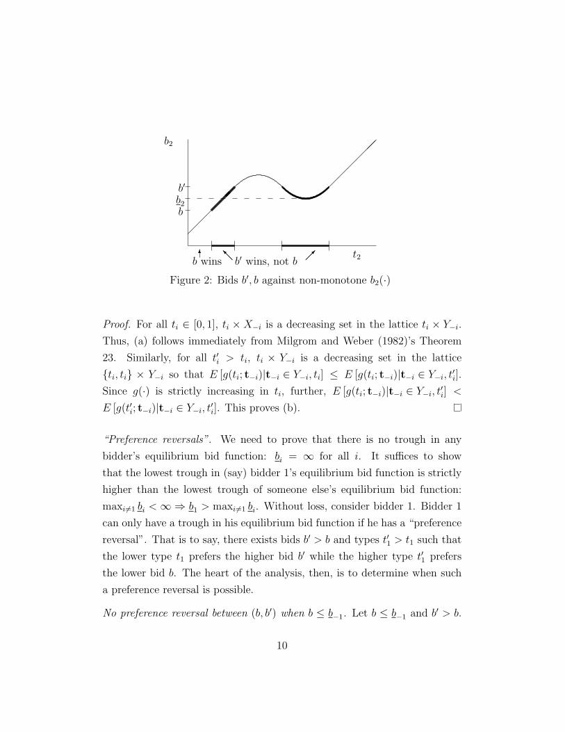
Figure 2: Bids b′, b against non-monotone b2(·)
Proof. For all ti ∈ [0, 1], ti × X−i is a decreasing set in the lattice ti × Y−i.
Thus, (a) follows immediately from Milgrom and Weber (1982)’s Theorem
23. Similarly, for all t′i > ti, ti × Y−i is a decreasing set in the lattice
{ti, ti} × Y−i so that E [g(ti; t−i)|t−i ∈ Y−i, ti] ≤ E [g(ti; t−i)|t−i ∈ Y−i, t′i].
Since g(·) is strictly increasing in ti, further, E [g(ti; t−i)|t−i ∈ Y−i, t′i] <
E [g(t′i; t−i)|t−i ∈ Y−i, t′i]. This proves (b).
“Preference reversals”. We need to prove that there is no trough in any
bidder’s equilibrium bid function: bi = ∞ for all i. It suffices to show
that the lowest trough in (say) bidder 1’s equilibrium bid function is strictly
higher than the lowest trough of someone else’s equilibrium bid function:
maxi6=1 bi < ∞⇒ b1 > maxi6=1 bi. Without loss, consider bidder 1. Bidder 1
can only have a trough in his equilibrium bid function if he has a “preference
reversal”. That is to say, there exists bids b′ > b and types t′1 > t1 such that
the lower type t1 prefers the higher bid b′ while the higher type t′1 prefers
the lower bid b. The heart of the analysis, then, is to determine when such
a preference reversal is possible.
No preference reversal between (b, b′) when b ≤ b−1. Let b ≤ b−1 and b′ > b.
10
Consider the trade-offs associated with bidding b′ versus b in terms of three
events, as illustrated in Figures 2, 3.
“b′ wins” ≡ {t−1 : maxj 6=1
bj(tj) < b′}
“b wins” ≡ {t−1 : maxj 6=1
bj(tj) < b}
“b′ wins, not b” ≡ {t−1 : maxj 6=1
bj(tj) ∈ (b, b′)}
(i) If t−1 ∈ “b wins”, then bidder 1 wins regardless of whether it bids b′ or b
and so clearly prefers to win with the lower bid. (ii) If t−1 ∈ “b′ wins, not b”,
then bidding b′ instead of b leads bidder 1 to win sometimes when b would
have lost. (iii) If t−1 6∈ “b′ wins”, then both bids lose and bidder 1 is clearly
For the purposes of applying Theorem 3(a,b) later, note that “b wins” is
11
decreasing in the lattice “b′ wins”. It will also be useful to partition “b′ wins”
into sets {ZJ : J ⊂ {2, ..., n}} defined by ZJ ≡ {t−1 : bi(ti) ∈ (b, b′) ∀i ∈J, bi(ti) < b ∀i 6∈ {2, ..., n}\J}. (Z∅ is the event “b wins”.) Note that ZJ is a
lattice and that Z∅ is decreasing in the lattice Z∅ ∪ ZJ for all J ⊂ {2, ..., n}.Figure 3 provides an example when n = 3 and bidders 2,3 follow a strategy
with a single trough as in Figure 2 such that b∗j(tj) ∈ [0, b) for all tj ∈ [0, t1j),
b∗j(tj) ∈ (b, b′) for tj ∈ (t1j , t2j)∪ (t3j , t
4j), and b∗j(tj) > b′ for tj ∈ (t2j , t
3j)∪ (t4j , 1].
(Z2, Z3, Z2,3 are not connected in Figure 3.)
Suppose for the sake of contradiction that b1 ≤ b−1 < ∞. This means
that there exists some pair of bids bh > bl and pair of types th1 > tl1 such that
(i) bl ≤ b−1, (ii) bh = b∗1(tl1), and (iii) bl = b∗1(t
h1).
2 In particular, EIU(tl1) ≥ 0
and EIU(th1) ≤ 0, where EIU(t1) is type t1’s expected incremental utility
prefers to bid slightly more given type t̂1 as long as doing so increases
its chances of winning.
(This argument applies for all tie-breaking rules since some bidder must ex-
pect to be able to increase its chances of winning by bidding b + ε. Further-
more, it can be adapted to the case in which bidder 2 adopts a non-monotone
strategy. For this reason, there can not be an equilibrium with positive prob-
ability of ties unless at least three bidders tie with positive probability.) Once
there are several bidders, however, it is not necessarily “good news” to learn
that one has tied with more bidders. For instance, when there are four or
more other bidders, I may prefer to win with bid b in the event that I tie with
two other bidders but prefer to lose if I tie with three other bidders, with
the further twist that my probability of winning depends on the number of
others that I tie with. This makes the issue of ruling out ties between three
or more bidders quite complex.
In the end, I prove in Theorem 4 that MR’s claim is correct in the context
of the coin-flip rule. Given that others have adopted monotone strategies,
your best response strategy will not lead you to tie with others with positive
probability. (The more general claim vis-a-vis all tie-breaking rules remains
to be verified and, indeed, may not be correct.)
Theorem 4: Given tie-breaking by coin-flip, ties occur with zero proba-
bility in every MPSE of the first-price auction.
Proof. Follows from Theorem 5 in the Appendix.
Theorems 1 and 4 leave open the possibility that there might be non-monotone
equilibria with a positive probability of ties. Now I demonstrate such an equi-
librium. It has the further property that all bidders and the auctioneer are
better off in this equilibrium than in any monotone one. One might expect
the presence of non-monotonicities to decrease the total surplus generated
by the auction since higher types bidding lower than lower types leads to
14
a more inefficient allocation. Another effect when some bidders adopt non-
monotone strategies, however, is that others face a weaker “winner’s curse”:
the expected value of the object conditional on winning with a low bid is
higher if others submit even lower bids when they have relatively high types.
This effect can increase total surplus if it leads to greater participation.
Example: Non-Monotone Equilibrium in the First-Price Auction
Three bidders i = 1, 2, 3 each have type ti ∈ {L, H}.3 These types (t1, t2, t3) =
t are affiliated and each bidder i’s valuation vi(t) for the object is non-
decreasing in t. After receiving its type, each bidder chooses whether to
participate and, if so, makes a bid bi ≥ pmin. The non-monotone equilibrium
I exhibit will have the form
b∗1(L) = pmin, b∗1(H) = OUT
b∗2(L) = pmin, b∗2(H) = OUT
b∗3(L) = OUT, b∗3(H) = pmin
Before fully specifying a concrete example it is helpful to examine the key
preference reversal, how bidder 1 (say) could prefer bidding pmin to OUT
upon receiving a low type but prefer OUT to pmin given a high type.
Ultimately, it must somehow be “bad news” for bidder 1 that she has
received a higher type that she then prefers to lose for sure rather than
sometimes win with bid pmin. To see how this could be the case, suppose for
the sake of argument that (i) bidder 1 doesn’t care about its own signal and
gets high value Vh > pmin from winning when t2 = H but a low value Vl <
pmin when t2 = L, that (ii) bidders 1,3 have somewhat positively correlated
types, and (iii) bidders 1,2 have independent types with (say) Pr(t2 = L) =
3Since all relevant bidder preferences are strict, one can easily modify the examplepresented here to fit within this paper’s model, i.e. to settings in which t is drawn froman atomless distribution on [0, 1]3 and in which bidder valuations are strictly increasingin own type, continuous, etc..
15
... with bid 100
t3L H
t2
L
H
50% 33%
100% 50%
... with bid 100 + ε
t3L H
t2
L
H
100% 100%
100% 100%
Figure 4: Probability that bidder 1 wins ...
50%. (In the example, condition (iii) is not satisfied but is assumed here
just to simplify the discussion.) Bidder 1’s probability of winning with bid
pmin is 100% if (t2, t3) = (H, L), 50% if (t2, t3) ∈ {(L, L), (H, H)}, and 33%
if (t2, t3) = (L, H), as summarized in Figure 4. Conditional on bidder 3
having a low type, bidder 1 assesses conditional probability Pr(t2 = H|t3 =
L, bidder 1 wins with bid pmin) = 100/(100+50) = 67% that the object has
a high value to her. On the other hand, when bidder 3 has a high type, this
conditional probability falls to 50/(50 + 33) = 60%. Thus, bidder 3’s having
a high type is bad news for bidder 1 vis-a-vis whether she wants to win with
bid pmin. Since t3 = H is more likely when t1 = H, having a high type herself
is bad news for bidder 1 unless the direct benefit associated with having a
higher type is large enough to offset this indirect effect.
Now to specifics. The joint probability of profile (L, L, L) = a, that
of (L, H, L) = (H, L, L) = b, etc.. where a, ..., f are determined by the
probability ratios b/a = c/b = d/c = 3/5, e/d = f/e = 2/3, as depicted in
Figure 5. t then is affiliated: as can be easily checked, a sufficient condition
for affiliation is that b/a ≤ c/b ≤ d/c ≤ e/d ≤ f/e. Note that t1, t2, t3
are independent when b/a = c/b = d/c = e/d = f/e, so this example is a
relatively small departure from the independent case, for which one can easily
16
t3 = L
t1L H
t2
L
H
a b
b c
t3 = H
t1L H
t2
L
H
d e
e f
Figure 5: Joint densities in ratio b/a = c/b = d/c = 3/5, e/d = f/e = 2/3
prove that all equilibria must be monotone. (Consequently, while bidders’
preferences are constructed to be strict, it is not surprising that some bidders
turn out to be nearly indifferent between bids OUT, pmin.)
Let pmin = 100. Bidders’ values for the object are non-decreasing in types.
Bidders 1,2 are symmetric and care only about the other’s type: v1(t) = 135
if t2 = H and v1(t) = 59 if t2 = L, and vice versa for bidder 2. Bidder 3
strictly prefers to win with bid 100 only if t1 = t2 = t3 = H. In particular,
v3(t) = 0 if t3 = L; otherwise, v3(t) = 70 if (t1, t2) = (L, L), v3(t) = 100 if
(t1, t2) ∈ {(L, H), (H, L)}, and v3(t) = 200 if (t1, t2) = (H, H).
Claim 1: bM(·) is a monotone equilibrium, where bM1 (L) = bM
1 (H) =
bM2 (L) = bM
2 (H) = bM3 (L) = OUT and bM
3 (H) = 100.
Proof. Bidders 1,2 are symmetric. Consider bidder 1. If he bids b > 100,
he wins the object and gets negative expected surplus given either t1 = L
since (135 − 100)(b + e) + (59 − 100)(a + d) < 0 or t1 = H since (135 −100)(c + f) + (59 − 100)(b + e) < 0. Similarly, if he bids b = 100, his
expected surplus conditional on winning is negative given either t1 = L since
(135−100)(b+e/2)+(59−100)(a+d/2) < 0 or t1 = H since (135−100)(c+
f/2) + (59 − 100)(b + e/2) < 0. Thus, his best response is always not to
17
participate. Consider bidder 3. Her best response must be either 100 or
OUT . Obviously t3 = L prefers OUT . The high type, however, gets positive
Finally, we determine best responses for bidder 3. Clearly she submits
the null bid when t3 = L. When t3 = H, any bid 100 + ε leads her to always
win for expected payoff approximately (110−100)(e+e+f)+(85−100)d > 0
since 10(2∗425
+ 875
)−15 625
= 23. To conclude the equilibrium verification, then,
I need to show that she prefers to submit 100 over any bid 100+ε. The payoff
to 100 is (110−100)( e2+ e
2+f)+(85−100)d
3= 10( 4
25+ 8
75)−15 2
25= 22
15> 2
3.
Claim 3: bNM(·) Pareto dominates bM(·).
Proof. Bidders 1,2 are better off since they now get positive utility upon
receiving low types. The auctioneer gets more revenue since now it sells the
object whenever t1 = L, t2 = L, or t3 = H. Bidder 3 is also better off since
she still always wins the object for sure in the good event (t1, t2) = (H, H)
but now only with probability 1/3 in the bad event (t1, t2) = (L, L).
There are several essential aspects to this example: (1) bidder values are not
private and (2) bidder types are not independent. Given either private values
or independent types, one can easily prove that ties can not occur in equilib-
rium. (It suffices to show that each bidder’s expected utility conditional on
tying is increasing in own value. Given private values, this is obvious. Given
independent signals, this follows from the fact that ex post utility is increas-
ing in own value.) (3) Some bidders adopt non-monotone strategies and ties
occur with positive probability. If bidders adopt monotone strategies, then
19
Theorem 4 shows that ties must occur with zero probability. Conversely,
if ties occur with zero probability, Theorem 1 implies that all bidders must
adopt monotone strategies. (4) Bidders are asymmetric. I have not man-
aged to prove this, but I believe that no non-monotone equilibrium can exist
given symmetric bidders. Some other aspects of the example may also be
important: (a) some bidders’ valuations are more sensitive to others’ types
than to their own and (b) ties occur exactly at the minimal permissible bid.
(If pmin = 100 − 2ε in the example below, bidder 1 would prefer to deviate
with bid 100 − ε since then it would only win the object in the event that
t2 = H, t3 = L.)
5 Concluding Remarks
When bidders have independent private values, it is well known that every
equilibrium in the first-price auction must be outcome-equivalent to some
monotone pure strategy equilibrium (“MPSE”). Once independence and/or
private values is relaxed, however, existing theory is silent on whether non-
monotone equilibria may exist. Yet in such models standard empirical iden-
tification approaches implicitly assume that monotone strategies are being
played. In a model allowing for asymmetric bidders, risk aversion, affiliated
types, and interdependent values, this paper provides the first theoretical
justification for restricting attention to monotone strategies. For one thing,
as discussed in the text, non-monotone equilibria can only exist in situations
in which both independence and private values are relaxed.
Suppose instead that one wishes to study a model having both affiliated
types and interdependent values. Given the coin-flip rule and a continuum
price grid, one can reject the possibility of non-monotone equilibria as soon
as one can reject the possibility that bidders tie with positive probability
(Theorem 1). In most empirical applications, of course, bids must be made
in discrete units so that ties can not be avoided. In such cases one can
20
still rule out non-monotone equilibrium a priori if ties are broken using the
priority rule (Theorem 2).
While my focus has been on asymmetric first-price auctions, all of the
results hold as well for symmetric models. In particular, as discussed in
the introduction, given existing results this paper proves that the symmetric
MPSE in Milgrom and Weber (1982)’s “general symmetric model” is in fact
its unique mixed strategy equilibrium. (More precisely, this is the unique
equilibrium under the priority rule and the unique equilibrium having zero
probability of ties under the coin-flip rule.)
Other tie-breaking rules than the coin-flip rule have been studied that
involve selecting a random winner. For instance, in their proof of MPSE
existence, Maskin and Riley (2000) make all tying bidders compete in a
second-price auction with the coin-flip rule to break further ties. My proof
approach does not extend to this tie-breaking rule nor does it apply to the
second-price auction. Indeed, Reny and Zamir (2004) provide an example
showing that all equilibria of the second-price auction may be non-monotone.
If bidders were to adopt such non-monotone strategies in Maskin and Riley
(2000)’s second bidding round, this might support non-monotone bidding in
the first round as well.
Lastly, it is worth noting some assumptions of the model that interesting
future work might attempt to relax:
One-dimensional types: Reny and Zamir (2004) provide a first-price auction
example with multi-dimensional affiliated types in which all equilibria are
non-monotone. In more specialized models that still allow for positively
correlated types, however, it remains an open question whether some or all
equilibria are monotone. In particular, existence of MPSE is unknown even
in symmetric first-price auctions given multi-dimensional affiliated types.
Affiliated types: Affiliation is a very strong distributional assumption which
has become widely used in the auction literature primarily for its analytical
21
convenience. The strong results derived here rest in large part on affiliation.
It remains an open question whether a weaker distributional assumption
suffices even for existence of MPSE.
Independent payoff-irrelevant signals: In the analysis here, bidders receive
independent payoff-irrelevant signals τ = (τ1, ..., τn). The conclusion that all
mixed strategy equilibria are outcome-equivalent to MPSE implies, among
other things, that bidders will never condition their bids on such signals. It
remains an open question whether bidders will ever condition their bids on
correlated payoff-irrelevant information.
Appendix
Proof of Theorem 1
The proof is divided into five parts. Most arguments to follow are framed in
terms of bidder 1 but, of course, they apply to all bidders.
Part I. No Ties at b if Strategies Monotone up to b. I begin with
several definitions, most of which are more general versions of definitions
made in the text:
Definition 11 (Less-than sets Wj(b), W∗j (b)): Type tj belongs to the
“sometimes less-than set” Wj(b) when it bids weakly less than b with positive
probability and belongs to the “always less-than set” W ∗j (b) when it never
bids more than b:
Wj(b) ≡{tj : Pr τj
(b∗j(tj; τj) ≤ b
)> 0}
,
W ∗j (b) ≡
{tj : Pr τj
(b∗j(tj; τj) ≤ b
)= 1}
,
Definition 12 (Lowest trough bj,b−j): The “lowest trough” of bid-
der j’s strategy, bj(b∗j(·; ·)) (shorthand bj), is the supremum of the set of bid
levels b such that, for all x < b, there exists t̃xj such that Wj(x) ⊂ [0, t̃xj ]
22
and W ∗j (x) ⊃ [0, t̃xj ). (This condition is satisfied vacuously for b = OUT so
that bj is well-defined.) Similarly, b−j ≡ mini6=j bi is the lowest lowest trough
across all other bidders.
Definition 13 (“Monotone up to b”): Bidder j’s strategy b∗j(·; ·)will be said to be “monotone up to b” when bj ≥ b.
Definition 14 (“No Ties at b”): There are “no ties at b” given strat-
egy profile b(·; ·) if Prt;τ (b = bj1(tj1 ; τj1) = bj2(tj2 ; τj2)) = 0 for all j1, j2. Sim-
ilarly, there are “no ties” if there are no ties at b for all b > OUT .
Theorem 5 (No Ties at b if Monotone up to b): Suppose that
b > OUT is a serious bid such that b∗j(·; ·) is monotone up to b for all bidders
j. Then there are no ties at b in the equilibrium b∗(·; ·).
Proof. Later in the Appendix.
Note that Theorem 5 implies Theorem 4 since any monotone equilibrium is,
by definition, monotone up to b for all bid levels b. In the example on page
15, ties occur with positive probability at b = 100. But b1 = b2 = OUT so
some strategies are not monotone up to 100.
Part II. Expected Payoffs Satisfy a Limited Strict Single-Crossing
Property: The standard approach to showing that all of bidder 1’s best re-
sponse strategies are monotone given independent private values is to show
that the expected incremental payoff from bidding higher satisfies strict
single-crossing in own type. That is to say, if t′1 > t1, b′ > b, and type t1
weakly prefers b′ over b, then type t′1 must strictly prefer b′ over b. Theorem
6 is the key result behind my proof, since it implies that expected incremen-
tal payoffs still satisfy strict single-crossing, though only with respect to a
limited set of pairs of bids and types.
Theorem 6 (Limited Strict Single-Crossing): For given bids b <
b′, suppose that some type t1 weakly prefers bid b′ over both bids b, OUT .
Furthermore, suppose that b∗(·; ·) has no ties at b′, that b′ is a serious bid,
23
and that b∗j(·; ·) is monotone up to b for all bidders j 6= 1. Then every type
t′1 > t1 strictly prefers bid b′ over both bids b, OUT .
Proof. Later in the Appendix.
Part III. Decreasing Less-Than Sets for Minimal Winning Bid R:
Let b∗(·; ·) be an equilibrium with no ties. A few definitions are useful for
specifying which bids have a chance of winning or of winning outright (i.e.
winning without tying) given others’ strategies.
Definition 15 (Rj, Rj, R): Define the closed convex hull of the support
of bidder j’s bid, Rj ≡ cl{b : Pr(b < b∗j(tj; τj)) ∈ (0, 1)}. Let Rj ≡ min Rj,
R−j ≡ maxi6=j Rj, and R ≡ maxj Rj.
Lemma 1 (Threshold type t̂1): In any equilibrium with no ties, thresh-
old type t̂1 exists such that (a) all types t1 > t̂1 get positive surplus and always
bid strictly greater than R−1 while (b) all types t1 < t̂1 get zero surplus and
always bid weakly less than R−1.
Proof. Consider a serious bid x = b∗1(t1, τ1), and define
Pr (“x wins”|t−1) ≡ Πj 6=1 Pr τj(b∗j(tj; τj) ≤ x)
(Recall that τ are independent.) For this x, define a “derived joint density
function” fx(·):
fx(t) = Pr (“x wins”|t−1) f(t) for all t ∈ [0, 1]n
(If a probability or expectation is not explicitly labelled otherwise, it is in-
tended to be taken with respect to the original density f .) Note that fx(·)is log-supermodular in t (LSPM) since both f(·) and Pr (“x wins”|t−1) are
LSPM. (f is LSPM since t are affiliated with respect to the original distribu-
tion; Pr (“x wins”|t−1) is LSPM since it is a product of terms Prτj(b∗j(tj; τj) <
x), each of which depends only on a one-dimensional variable tj and hence is
24
automatically log-supermodular.) Thus t are affiliated with respect to a new
joint distribution having density fx(·) over [0, 1]n and a probability mass at
(say) (2, ..., 2) of 1−∫t∈[0,1]n
fx(t)dt.
Bidder 1’s expected payoff to bidding x can be easily expressed in terms
of expectations taken with respect to fx(·). First, given type t1, bidder 1’s
expected payoff conditional on winning outright equals
Efx [(u1(t, x)) |t1] = Ef
[(u1(t, x)) Πj 6=1 Pr τj
(b∗j(tj; τj) < x
)|t1]
Since type t1 bids x, no ties implies that at most one other bidder (call it h∗)
bids exactly x with positive probability. If there is no such bidder, we may
ignore ties at x; else let H denote the event in which bidder 1 would tie with
bidder h∗ by bidding b:
H ≡{th∗ : Pr τh∗ (b∗h∗(th∗ ; τh∗) = x|t1) > 0}×
×∏
j 6=1,h∗
{tj : Pr
τj
(b∗j(tj; τj) < x|t1
)> 0
}Furthermore, bidder 1’s incremental expected payoff (in the limit as ε → 0)
from bidding x + ε versus x as well as between bidding x versus x− ε must
equal VH/2, where
VH = Efx
[u1(t, x) Pr τh∗
(b∗h∗(th∗ , τh∗) = x
∣∣b∗h∗(th∗ , τh∗) ≤ x)∣∣∣∣t1, t−1 ∈ H
]Thus, x can only be preferred to both x − ε and x + ε if VH = 0. In other
words, bidder 1’s expected payoff conditional on tying must be zero. Since
non-participation OUT gives guaranteed zero payoff, bidder 1’s type t1 must
therefore get non-negative payoff from winning outright with bid x, i.e.
0 ≤ Efx [u1(t, x)|t1](1)
Since u1(·) is strictly increasing in t1, Theorem 3(b) applied to (1) implies
that Egx [u1(t)|t1] is strictly increasing in t1. Consequently, for all t′1 > t1
25
bidder 1’s payoff to bidding x in the event of winning outright is strictly
positive. Similarly, since H is a lattice, types t′1 > t1 must get non-negative
expected utility conditional on tying, so that all together such types get
positive expected payoff from bidding x. This implies, of course, that such
types must always bid strictly greater than R−1: by definition, a bid less than
or equal to R−1 never wins outright; and, in equilibrium with ties against at
most one other bidder, one’s expected payoff from winning by tying with bid
R−1 must be zero.
Define t̂1 ≡ inf{t1 : Prτ1
(b∗1(t1; τ1) > R−1
)> 0}. Since all types t′1 > t1
always bid greater than R−1 if ever type t1 bids greater than R−1, (a) all
types t1 > t̂1 get positive surplus and always bid strictly greater than R−1
while (b) all types t1 < t̂1 get zero surplus and always bid weakly less than
R−1.
It will be useful later in the proof to observe that there is a bidder j∗ for
whom t̂j∗ = 0. Proof: If i = arg maxj Rj then set i = j∗. Otherwise, suppose
that all bidders in arg maxj Rj bid R with positive probability. In this case,
they would tie with positive probability at R, contradicting the assumption
of no ties. So at least one of these bidders must bid R with zero probability.
This bidder is our j∗.
Definition 16 (Bidder j∗): j∗ is a bidder such that j∗ ∈ arg maxj Rj
and tj∗ = 0.
Bidder j∗ always wins outright with positive probability given any type tj∗ >
0. Furthermore, this lowest type tj∗ = 0 wins outright in the event that
tj < t̂j for all j 6= j∗. (This event may or may not have positive probability.)
Part IV. Strategies Monotone up to R. Part III showed that all types
tj < t̂j lose with probability one while all types tj > t̂j win outright with
positive probability. Yet types tj < t̂j are indifferent between all always-
losing bids and hence could submit any always-losing bid (or mix over several
such bids) in equilibrium. While these bids never win, it is conceivable that
26
such bidding behavior might support others’ equilibrium strategies. As it
turns out, however, this is not the case. We may assume without loss that
bidders adopt monotone strategies over the range of always-losing types.
Lemma 2 (Strategies monotone up to R): Every mixed strategy
equilibrium b∗(·; ·) that has no ties at all bid levels has an outcome-equivalent
equilibrium b̃(·; ·) in which each bidder j’s strategy is monotone up to R.
Proof. Consider any new strategy profile b̃(·; ·) that satisfies three require-
ments: for all bidders j,
(i) b̃j(tj; τj) = b∗j(tj; τj) for all tj > t̂j and all τ : The sometimes-winning
types bid the same as in the original equilibrium.
(ii) Pr(b̃j(tj; τj) ≥ maxi6=j b̃i(ti; τi)
)= 0 for all tj < t̂j and all τ : The
always-losing types still always lose.
(iii) b̃j(tj; τ′j) = b̃j(tj; τj) ≡ b̃j(tj) for all tj < t̂j, τ ′,τ , and b̃j(tj) ≤ b̃j(t
′j) for
all tj < t′j < t̂j: Monotone pure strategy over the range of always-losing
types.
In the three cases below (a,b,c), I modify the original equilibrium strategies in
different ways but in each case the new strategies satisfy conditions (i,ii,iii).
By (i,ii) the new strategy profile is outcome-equivalent to the original
equilibrium. Each bidder’s payoffs (and preferences) over the range of bids
greater than R, furthermore, remains the same. Since j∗ always bids at
least R in the original equilibrium, lastly, everyone else is indifferent between
the null-bid and any bid less than R. So, every bidder j 6= j∗ still finds
her new strategy to be a best response and bidder j∗’s preferences amongst
bids greater than R remain the same. The new strategy profile then is an
equilibrium itself unless some bidder j∗-type now prefers to bid weakly less
than R who previously bid more than R or now prefers to bid strictly less
than R who previously bid exactly R.
27
There are three cases to consider:
(a) Some bidder j 6= j∗ bids exactly R with positive probability in the
original equilibrium. But then to avoid ties j∗ must bid strictly greater than
R with probability one. Consider modified strategies b0(·; ·):
b0j(tj; τj) = b∗j(tj; τj) for all j, tj > t̂j, τj
b0j(tj; τj) = R for all j, tj ≤ t̂j, τj
(Bidder j∗’s strategy is unchanged4 and all other bidders’ strategies remain
the same for types tj > t̂j.) Any bidder j∗-type certainly will not choose
to bid strictly less than R now since that guarantees no chance of winning
and hence zero payoff. Bidding exactly R might allow bidder j∗ to win with
positive probability, but only by tying with all of the other bidders. By the
proof of Theorem 5, however, bidder j∗ can only weakly prefer bidding R
over both R + ε, OUT (for all small ε) if she gets zero expected utility from
bidding R, again no better than the payoff from her original equilibrium bid.
Thus, b0(·; ·) is an equilibrium that is monotone up to R.
(b) No bidder j 6= j∗ bids exactly R with positive probability and R =
R−j∗ , i.e. some other bidder j′ 6= j∗ also never bids less than R. In this
case, any strategy profile satisfying requirements (i,ii,iii) will be an outcome-
equivalent equilibrium that is monotone up to R: Bidder j∗ has no chance of
winning with a bid less than or equal to R so bidding behavior at and below
R is irrelevant to bidder j∗’s best response. (For example, using strategies
b(4,β)j (·; ·) defined below would work.)
(c) No bidder j 6= j∗ bids exactly R with positive probability and R >
R−j∗ . In this last and most difficult case, all bidder j∗-types win with positive
probability in the original equilibrium. If R = pmin, then all types tj ∈ [0, t̂j)
must be bidding OUT for all j 6= j∗, and so b∗(·; ·) is monotone up to R
4To keep the proof relatively readable, I do not explicitly keep track of changes thatoccur on zero measure sets of types. All references to “no types” or “all types” should beunderstood as being made modulo a zero measure set.
28
tj
bj
pmin
OUT
R−4R− βt̂j
t̂j
R
��
��
���
��
���
���
r r rrrrrrrbbbbbb rrrrrr
Figure 6: Graph of original equilibrium strategy traced by solid line; graph
of new strategy b(4,β)j (·) traced by filled circles
already. If R > pmin, consider a family of modified strategies (indexed by
4 ∈ (0, R− pmin] and β ∈ (0, (R− pmin)/t̂j]):
b(4,β)j (tj; τj) = b∗j(tj; τj) for all j, tj > t̂j, τj
b(4,β)j (tj) = R−
(t̂j − tj
)β for all j, tj ∈
[max{0, t̂j −4/β}, t̂j
]= R−4 for all j, tj < max{0, t̂j −4/β}
as illustrated in Figure 6. First, note that bidder j∗’s payoff to bidding
exactly R remains the same as in the original equilibrium, so it remains for
us only to rule out the possibility that some j∗-type who bid weakly greater
than R before now prefers to bid strictly less than R.
My claim is that, for small enough (4, β), no bidder j∗-type has incentive
to bid strictly below R. To see this note that, since b(4,β)j (tj; τj) is monotone
up to R (for all j 6= j∗), Theorem 6 implies that if type tj∗ = 0 weakly prefers
b′ > R over b ≤ R given these new strategies, then all types tj∗ > 0 must
strictly prefer b′ over b. Thus, it suffices for me to show that the lowest type
tj∗ = 0 does not strictly prefer to bid strictly less than R. The rest of this
29
part of the proof focuses on this single type.
For given (4, β), all bids less than p4,β ≡ max{R−4, R− t̂jβ} lose for
certain and so can not be strictly preferred by type tj∗ = 0 over its original
equilibrium bid. Type tj∗ = 0’s utility from bidding b ∈ [p4,β, R] takes the
form
πβ(b) = P β(b, 0)V β(b, b, 0) where
P β(b2, b1) ≡ Pr
(maxj 6=j∗
b4,βj (tj) ∈ [b1, b2]
∣∣∣tj∗ = 0
)V β(b′, b2, b1) ≡ E
(uj∗(t, b
′)∣∣tj∗ = 0, max
j 6=j∗b4,βj (tj) ∈ [b1, b2] for all j 6= j∗
)P β(b2, b1) is the probability that the highest bid by bidders −j∗ is in [b1, b2].
(For small enough β this doesn’t depend on 4.) P β(b, 0) is the probability
that b is high enough to win. Similarly, V β(b′, b2, b1) is type tj∗ = 0’s expected
utility from paying b′ for the object conditional on the highest bid by bidders
−j∗ being in [b1, b2]. In particular, V β(b′, b, OUT ) is type tj∗ = 0’s expected
utility from paying b′ for the object conditional on b being high enough to
win.
Note that, by design,
V β1(R, R− β1x, OUT ) = V β2(R, R− β2x, OUT ) for all β1, β2 > 0, x ≥ 0
(2)
P β1(R− β1x, OUT ) = P β2(R− β2x, OUT ) for all β1, β2 > 0, x ≥ 0(3)
Before proceeding, I need to establish some smoothness properties of these
functions. First, by (A1) the joint density f(·) is measurable so P β(b, OUT )
is continuous in b at R. Since P β(b, OUT ) is also non-decreasing in the
bid, the left-derivative P β1 (R, OUT ) ≥ 0 is well-defined. Similarly, by (A3)
utility is measurable in types so that V β(b′, b, OUT ) is continuous in b and
utility is continuous in bid so that V β(b′, b, OUT ) is differentiable in b′ (with
V β1 (R, R, OUT ) < 0). Finally, since the strategies b
(4,β)j (·; ·) are monotone
up to R, V β(b′, b, OUT ) is non-decreasing in b as long as b ≤ R. Together
30
with continuity, then, we have that the left-derivative V β2 (R, R, OUT ) ≥ 0 is
well-defined.
Next, using equations (2, 3), observe that
P β2
1 (R, OUT ) = β1/β2Pβ1
1 (R, OUT ) for all β1, β2
V β2
1 (R, R, OUT ) = V β1
1 (R, R, OUT ) for all β1, β2
V β2
2 (R, R, OUT ) = β1/β2Vβ1
2 (R, R, OUT ) for all β1, β2
(The smaller β, the more probability mass gets “stacked up” just below R.
This also affects the rate at which bidder j∗’s expected value from winning
decreases as he lowers his bid, though not the rate at which lowering his bid
decreases his expected payment.)
Figure 7 provides an illustration of type tj∗ = 0’s expected utility from
submitting various bids both under the original equilibrium (solid line) as
well as under strategies b(4,β) (trace of circles for b < R; solid line for
b ≥ R) in the most difficult case when j∗ was originally indifferent between
her equilibrium bid and some bid less than R.5 By construction all bids less
than p4,β lose for certain, get zero utility, and can not be strictly preferred
to any equilibrium bid. What we need to show is that type tj∗ = 0’s utility
is increasing in her bid in a neighborhood to the left of R, i.e. that the
(left-)derivative π1(R) ≥ 0 where
π1(R) ≡P β1 (R, OUT )V β(R, R, OUT )(4)
+ P β(R, OUT )(V β
1 (R, R, OUT ) + V β2 (R, R, OUT )
)Given small enough 4, then, no bid less than R can be preferred to R (and
hence to its original equilibrium bid).
Suppose first that V β(R, R, OUT ) > 0. Since V β1 (R, R, OUT ) is bounded
and V β2 (R, R, OUT ) ≥ 0, we may choose β small enough that P β
1 (R, OUT )
is large enough that π1(R) > 0.
5In the Figure, type tj∗ = 0 does not randomize and its equilibrium bid is strictlygreater than R. Neither feature is needed for the argument.
31
bj∗
utility of tj∗ = 0
R−j∗
p4,��
b∗j∗(tj∗)R
������
bbbbbbbbbb
Figure 7: Graph of j∗’s utility from various bids; changes induced by strategy
modifications traced by circles.
Suppose next that V β(R, R, OUT ) = 0. In this case, it suffices to show
that V β2 (R, R, OUT ) > 0 since then we may choose β small enough that
V β2 (R, R, OUT ) is large enough that π1(R) > 0. For this purpose, observe
that for any b1 < R,
P β(R, OUT )V β(R, R, OUT ) = P β(b1, OUT )V β(R, b1, OUT )+P β(R, b1)V β(R, R, b1)
or re-arranging,
V β(R, R, OUT )−V β(R, b1, OUT ) =P β(R, b1)
(V β(R, R, b1)− V β(R, b1, OUT )
)P β(R, OUT )
So, V β2 (R, R, OUT ) = 0 only if V β(R, R, R) = V β(R, R, OUT ). By Theorem
3, however, V β(R, R, R) = V β(R, R, OUT ) only if bidder j∗’s value for the
object is constant in t−j∗ over the whole event{tj ≤ t̂j for all j 6= j∗
}, i.e.
only if bidder j∗ has “private values” over this range of others’ type profiles.
In this case, however, to deter bidder j∗ from wanting to deviate with a bid
below R, all we need to do is make sure that her probability of winning with
any such bid is less than it was under the original equilibrium strategies.
This can be done by making β sufficiently small. This completes the proof
that any mixed-strategy equilibrium has an outcome-equivalent equilibrium
that is monotone up to R.
32
Part V. Putting It All Together: By Lemma 2, we may assume that each
bidder’s strategy is monotone up to R. To prove that every equilibrium must
be monotone, it suffices to show that b1 > minj 6=1 bj ≡ b−1 whenever b−1 < ∞.
Suppose for the sake of contradiction that R ≤ b1 ≤ b−1 < ∞. This requires
that, in equilibrium, there exists bid b′ > b−1 and types t′1(ε), t1 such that
type t1 bids b′ and each type t′1(ε) > t1 bids b(ε) < b−1 + ε. First note that it
must be that b(ε) > b−1 for all ε. Otherwise, since all bidders’ strategies are
monotone up to b−1 and by assumption there are no ties, Theorem 6 implies
that all types greater than t1 must strictly prefer b′ over b(ε) if type t1 weakly
prefers b′ over b(ε), a contradiction.
Without loss, also, we may assume that type t′1 exists such that t′1(ε) ∈(t′1 − ε, t′1 + ε) for all small enough ε.6 Define a sequence of functions
γεk(t−1, τ−1) ≡ u1 (t′1(εk), t−1, b(εk)) if maxj 6=1
b∗j(tj; τj) < b(εk)
≡ 0 otherwise
γεk is bidder 1’s ex post payoff from bidding b(εk) when he has type t′1(εk).
Note that γεk converges almost surely to γ0 defined as
γ0(t−1, τ−1) ≡ u1
(t′1, t−1, b−1
)if max
j 6=1b∗j(tj; τj) ≤ b−1
≡ 0 otherwise
Consider ‘hypothetical’ bid b+−1 defined by b−1 < b+
−1 < b′ for all b′ > b−1.
γ0 corresponds to bidder 1’s ex post payoff from submitting bid b+−1 given
limiting type t′1. Since utilities are bounded, we may apply the bounded
convergence theorem to conclude that
limk→∞
Et−1,τ−1
[γεk(t−1, τ−1)
∣∣t′1] = Et−1,τ−1
[γ0(t−1, τ−1)
∣∣t′1] ,6Let t′1 be any accumulation point of a sequence {t′1(εk)}∞k=1 such that εk → 0. Then
we have that, for all ε, some type in (t′1 − ε, t′1 + ε) bids b(ε) ∈(b−1, b−1 + ε
).
33
i.e. type t′1 must at least weakly prefer bidding b+−1 to b′. On the other hand,
by assumption type t1 chose to bid b′ rather than any bid in a neighborhood
(b−1, b−1 + ∂), implying (by continuity of utility in the bids) that this lower
type must weakly prefer b′ over b+−1. Finally, by Lemma 1, the set of t−1
profiles against which b+−1 would win is a decreasing set and a lattice and that
(by definition of this ‘hypothetical’ bid) no other bidder ever bids exactly b+−1.
Thus, Theorem 6 implies that any type greater than t1 must strictly prefer
b′ to b+−1, a contradiction. This completes the proof of Theorem 1.
Proof of Theorem 2
Redefine the grid of permissible bids as follows: each bidder j submits a bid
from the set (OUT ∪ P) × ρ(j) where (OUT ∪ P) × {1, ..., n} is endowed
with the lexicographic order (p′, k′) > (p, k) iff p′ > p or p′ = p, k′ > k. Now,
define the lowest trough of each bidder’s strategy in terms of this richer bid
space and no two lowest troughs can be equal – by definition! All five parts
of Theorem 1 proof go through with only minor changes (though several
of the most challenging parts of the proof become irrelevant since ties at
always-losing bid levels are no longer possible).
Proof of Theorem 5 (and hence Theorem 4)
Since each bidder’s strategy is monotone up to b, there exists a threshold
type t̂bj such that Pr(b∗j(tj; τj) < b) = 1 for all tj < t̂bj and Pr(b∗j(tj; τj) <
b) = 0 for all tj > t̂bj. One can summarize this by saying that bidder j
always bids less than b when tj ∈ [0, t̂bj) and bids equal to b with probability
Prτj
(b∗j(tj; τj) ≤ b|tj
)when tj ∈ (t̂bj, 1]. One may then characterize bidder 1’s
expected payoff from bidding b conditional on type t1 (shorthand π1(b, t1))
as
π1(b, t1) ≡∫
[0,1]n−1
1
1 + #(j 6= 1 : tj > t̂bj
) (u1(t, b)) f b(t−1|t1)dt−1
34
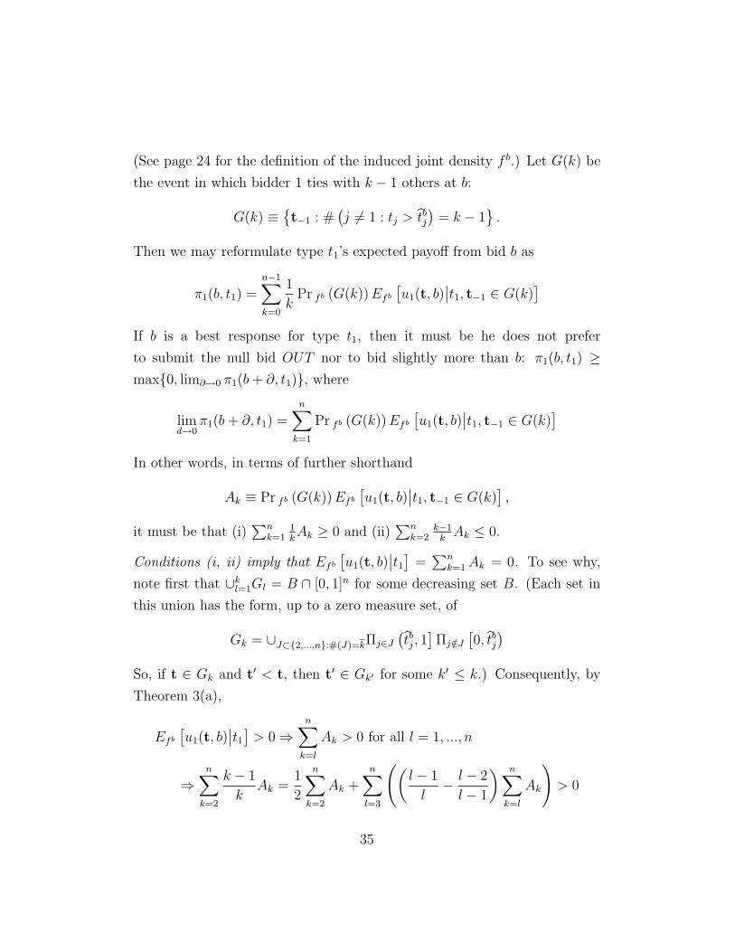
(See page 24 for the definition of the induced joint density f b.) Let G(k) be
the event in which bidder 1 ties with k − 1 others at b:
G(k) ≡{t−1 : #
(j 6= 1 : tj > t̂bj
)= k − 1
}.
Then we may reformulate type t1’s expected payoff from bid b as
π1(b, t1) =n−1∑k=0
1
kPr fb (G(k)) Efb
[u1(t, b)
∣∣t1, t−1 ∈ G(k)]
If b is a best response for type t1, then it must be he does not prefer
to submit the null bid OUT nor to bid slightly more than b: π1(b, t1) ≥max{0, lim∂→0 π1(b + ∂, t1)}, where
limd→0
π1(b + ∂, t1) =n∑
k=1
Pr fb (G(k)) Efb
[u1(t, b)
∣∣t1, t−1 ∈ G(k)]
In other words, in terms of further shorthand
Ak ≡ Pr fb (G(k)) Efb
[u1(t, b)
∣∣t1, t−1 ∈ G(k)],
it must be that (i)∑n
k=11kAk ≥ 0 and (ii)
∑nk=2
k−1k
Ak ≤ 0.
Conditions (i, ii) imply that Efb
[u1(t, b)
∣∣t1] =∑n
k=1 Ak = 0. To see why,
note first that ∪kl=1Gl = B ∩ [0, 1]n for some decreasing set B. (Each set in
this union has the form, up to a zero measure set, of
Gk = ∪J⊂{2,...,n}:#(J)=kΠj∈J
(t̂bj, 1
]Πj /∈J
[0, t̂bj
)So, if t ∈ Gk and t′ < t, then t′ ∈ Gk′ for some k′ ≤ k.) Consequently, by
Theorem 3(a),
Efb
[u1(t, b)
∣∣t1] > 0 ⇒n∑
k=l
Ak > 0 for all l = 1, ..., n
⇒n∑
k=2
k − 1
kAk =
1
2
n∑k=2
Ak +n∑
l=3
((l − 1
l− l − 2
l − 1
) n∑k=l
Ak
)> 0
35
Thus, Efb
[u1(t, b)
∣∣t1] ≤ 0. On the other hand, Efb
[u1(t, b)
∣∣t1] ≥ 0 since
Efb
[u1(t, b)
∣∣t1] < 0 ⇒l∑
k=1
Ak < 0 for all l = 1, ..., n
⇒n∑
k=1
1
kAk =
1
n
n∑k=1
Ak +n−1∑l=1
((1
l− 1
l + 1
) l∑k=1
Ak
)< 0
Finally, by Theorem 3(b) Efb
[u1(t, b)
∣∣t1] is strictly increasing in t1. We may
conclude then that at most one bidder type t1 bids b in equilibrium if all
others’ bids are monotone up to b.
Proof of Theorem 6
First, there are no ties at b by Theorem 5. Furthermore, since by assumption
each bidder j 6= 1 adopts a strategy that is monotone up to b,the event
“b wins” ≡ Πj 6=1Wj(b) in which bidder 1 can sometimes win with bid b is
decreasing and the same (up to a zero measure set) as the event Πj 6=1W∗j (b)
in which bidder 1 always wins with bid b. Similarly, define “b′ wins” ≡Πj 6=1Wj(b
′). Since “b′ wins” is a lattice,
E[u1(t, b
′)∣∣t′1, t−1 ∈ “b′ wins”
]> E
[u1(t, b
′)∣∣t1, t−1 ∈ “b′ wins”
]≥ 0
where the first inequality follows from Theorem 3(b) and the second from
the assumption that type t1 weakly prefers b′ to OUT . Thus, type t′1 strictly
prefers b′ to OUT . Now we need to show that type t′1 strictly prefers b′ to b.
Suppose for the sake of contradiction that t′1 weakly prefers b to b′.
For every J ⊂ {2, ..., n}, define XJ to be the set of others’ type profiles
so that all bidders j ∈ J submit a bid in (b, b′) and all bidders j 6∈ J bid less
than b:
XJ ≡ Πj∈J (Wj(b′)\Wj(b)) Πj∈{2,...,n}\JWj(b)
Each set XJ is a lattice, where X∅ = “b wins” and the union of all of these
sets is “b′ wins”. Furthermore, for all J 6= ∅, X∅ ∪ XJ is a lattice in which
X∅ is decreasing.
36
Type t1’s incremental payoff to bidding b′ versus b depends on whether
bid b and/or b′ win. Conditional on b winning, bidding b′ leads to a (negative)
incremental gain of u1(t, b′)−u1(t, b); conditional on b′ winning and b losing,
bidding b′ leads to an incremental gain equal to the expected utility from
winning and paying b′. Define
φ1(t−1) ≡ u1(t, b′)− u1(t, b) if t−1 ∈ X∅
≡ Efb′[u1(t, b
′)|t′1, t−1 ∈ XJ]
whenever t−1 ∈ XJ
≡ 0 otherwise
(See page 24 for the definition of the density function f b′(·).) φ1(t−1) is
the ex post incremental payoff to type t′1; Efb′[φ1(t−1)|t̂1
]> 0 iff bidder 1
would get positive expected incremental payoff from bidding b′ over b in a
hypothetical situation in which she got ex post payoffs like type t′1 but others’
types were distributed as if she had type t̂1. Consequently,
Efb′ [φ1(t−1)|t′1] ≤ 0, Efb′ [φ1(t−1)|t1] ≥ 0
The first inequality states that type t′1 weakly prefers bid b over b′; the second
inequality follows from the facts that type t1 weakly prefers bid b′ over b and
that type t′1’s ex post incremental payoff to bidding b′ over b is never less than
type t1’s. On the other hand, Theorem 3(a) implies that Efb′ [φ1(t−1)|t′1] > 0
if φ1(·) is a non-decreasing function over the lattice “b′ wins”. In other words,
to achieve a contradiction we need only show that, for all J ′ ⊃ J 6= ∅,
Efb′
[u1(t, b
′)|t′1, t−1 ∈ XJ ′]≥ Efb′
[u1(t, b
′)|t′1, t−1 ∈ XJ]
(5)
Efb′
[u1(t, b
′)|t′1, t−1 ∈ XJ ′]≥ Efb′
[u1(t, b
′)− u1(t, b)|t′1, t−1 ∈ X∅](6)
Equation (5) follows immediately from Theorem 3(a) since XJ is a decreasing
set in the lattice XJ ∪ XJ ′ . For equation (6), note again by Theorem 3(a)
that
Efb′[u1(t, b
′)|t′1, t−1 ∈ XJ]≥ Efb′
[u1(t, b
′)|t′1, t−1 ∈ X∅]37
Thus it suffices to show that Efb′[u1(t, b)|t′1, t−1 ∈ X∅] ≥ 0. But this follows
directly from the presumption that type t′1 weakly prefers bid b over the
null-bid.
References
Hendricks, K., J. Pinkse, and R. Porter (2003): “Empirical Impli-
cations of Equilibrium Bidding in First-Price, Symmetric, Common Value
Auctions,” Review of Economic Studies, 70(1), 115–146.
Kagel, J., and D. Levin (2002): Common Value Auctions and the Win-
ner’s Curse. Princeton University Press.
Maskin, E., and J. Riley (2000): “Equilibrium in Sealed High-Bid Auc-
tions,” Review of Economic Studies, 67, 439–454.
McAdams, D. (2004): “Uniqueness in Symmetric First-Price Auctions with
Affiliation,” manuscript, available at http://www.mit.edu/˜mcadams.
Milgrom, P., and R. Weber (1982): “A Theory of Auctions and Com-