1 IntroductionCompressed sensing is a modern paradigm of data acquisition, which is having
an impact on several disciplines; see [21]. The scientist has access to a measure-ment vector v 2 Rm obtained as
(1.1) v D Ax;
where A is a given m � n measurement matrix and x 2 Rn is an unknown signalthat one needs to recover from v. One would like to take m � n, rendering A
noninvertible; the key ingredient to successful recovery of x is to take into accountits assumed structure—sparsity. Thus one assumes that x has at most s nonzeroentries, although the support pattern is unknown. The strongest known resultsare for random measurement matrices A. In particular, if A has Gaussian i.i.d.entries, then we may takem D O.s log.n=s// and still recover x exactly with highprobability [8, 9]; see [26] for an overview. Furthermore, this recovery may beachieved in polynomial time by solving the convex minimization program
(1.2) min kx0k1 subject to Ax0 D v:
Stability results are also available when noise is added to the problem [3, 7, 10, 27].However, while the focus of compressed sensing is signal recovery with minimal
information, the classical setup (1.1)–(1.2) assumes infinite bit precision of themeasurements. This disaccord raises an important question: how many bits per
measurement (i.e., per coordinate of v) are sufficient for tractable and accuratesparse recovery? This paper shows that one bit per measurement is enough.
There are many applications where such severe quantization may be inherent orpreferred—analog-to-digital conversion [18, 20] and binomial regression in statis-tical modeling and threshold group testing [12], to name a few.
1.1 Main ResultsThis paper demonstrates that a simple modification of the convex program (1.2)
is able to accurately estimate x from extremely quantized measurement vector
y D sign.Ax/:
Here y is the vector of signs of the coordinates of Ax.1
Note that y contains no information about the magnitude of x, and thus wecan only hope to recover the normalized vector x=kxk2. This problem was intro-duced and first studied by Boufounos and Baraniuk [6] under the name of one-bitcompressed sensing; some related work is summarized in Section 1.2.
We shall show that the signal can be accurately recovered by solving the follow-ing convex minimization program:
(1.3) min kx0k1 subject to sign.Ax0/ � y and kAx0k1 D m:
The first constraint, sign.Ax0/ � y , keeps the solution consistent with the mea-surements. It is defined by the relation hai ;x0i � yi � 0 for i D 1; : : : ; m, whereai is the i th row of A. The second constraint, kAx0k1 D m, serves to prevent theprogram from returning a zero solution. Moreover, this constraint is linear as it canbe represented as one linear equation
PmiD1 yi hai ;x
0i D m where the yi denotethe coordinates of y . Therefore (1.3) is indeed a convex minimization program;furthermore, one can easily represent it as a linear program; see (5.3) below. Notealso that the number m in (1.3) is chosen for convenience of the analysis; it can bereplaced by any other fixed positive number.
THEOREM 1.1 (Recovery from One-Bit Measurements). Let n;m; s > 0, and let A
be an m � n random matrix with independent standard normal entries. Set
(1.4) ı D C� sm
log.2n=s/ log.2n=mC 2m=n/�1=5
:
Then, with probability at least 1�C exp.�cım/, the following holds uniformly forall signals x 2 Rn satisfying kxk1=kxk2 �
ps: Let y D sign.Ax/. Then the
solution yx of the convex minimization program (1.3) satisfies yx
kyxk2�
x
kxk2
2
� ı:
Here and hereafter C and c denote positive absolute constants; other standardnotation is explained in Section 1.3.
1 To be precise, for a scalar ´ ¤ 0 we define sign.´/ D ´=j´j and sign.0/ D 0. We allow the signfunction to act on a vector by acting individually on each element.
1-BIT CS BY LINEAR PROGRAMMING 1277
Remark 1.2 (Effective Sparsity). The Cauchy-Schwarz inequality implies thatkxk1
kxk2�pkxk0
where kxk0 D jsupp.x/j is the number of nonzero elements of x. Thereforeone can view the parameter .kxk1=kxk2/2 as a measure of effective sparsity ofthe signal x. The effective sparsity is thus a real valued and robust extension of thesparsity parameter kxk0, which allows one to handle approximately sparse vectors.
Let us then state the partial case of Theorem 1.1 for sparse signals:
COROLLARY 1.3 (Sparse Recovery from One-Bit Measurements). Let n;m; s > 0,and set ı as in (1.4). Then, with probability at least 1�C exp.�cım/, the followingholds uniformly for all signals x 2 Rn satisfying kxk0 � s. Let y D sign.Ax/.Then the solution yx of the convex minimization program (1.3) satisfies yx
kyxk2�
x
kxk2
2
� ı:
Remark 1.4 (Number of Measurements). The conclusion of Corollary 1.3 can bestated in the following useful way: With high probability, an arbitrarily accurateestimation of every s-sparse vector x can be achieved from
m D O.s log2.n=s//
one-bit random measurements. The implicit factor in the O.�/ notation dependsonly on the desired accuracy level ı; more precisely, m � ı�5s log2.n=s/ up toan absolute constant factor. The same holds if x is only effectively s-sparse as inTheorem 1.1. The central point here is that the number of measurements is almostlinear in the sparsity s, which can be much smaller than the ambient dimension n.
Remark 1.5 (Non-Gaussian Measurements). Most results in compressed sensing,and in random matrix theory in general, are valid not only for Gaussian randommatrices but also for general random matrix ensembles. In one-bit compressedsensing, since the measurements sign.Ax/ do not depend on the scaling of therows of A, it is clear that our results will not change if the rows of A are sampledindependently from any rotationally invariant distribution in Rn (for example, theuniform distribution on the unit euclidean sphere Sn�1).
However, in contrast to the widespread universality phenomenon, one-bit com-pressed sensing cannot be generalized to some of the simplest discrete distribu-tions, such as Bernoulli. Indeed, suppose the entries of A are independent ˙1valued symmetric random variables. Then for the vectors x D .1; 0; 0; : : : ; 0/ andx0 D .1; 1
2; 0; : : : ; 0/ one can easily check that sign.Ax/ D sign.Ax0/ for any
number of measurements m. So one-bit measurements cannot distinguish betweentwo fixed distinct signals x and x0 no matter how many measurements are taken.
Remark 1.6 (Optimality). For a fixed level of accuracy, our estimate on the num-ber of measurements m D O.s log2.n=s// matches the best known number of
1278 Y. PLAN AND R. VERSHYNIN
measurements in the classical (not quantized) compressed sensing problem up tothe exponent 2 of the logarithm, and up to an absolute constant factor. How-ever, we believe that the exponent 2 can be reduced to 1. We also believe thatthe error ı in Theorem 1.1 may decrease more quickly as s=m ! 0. In par-ticular, Jacques et al. [18] demonstrate that x is exactly sparse and is estimatedusing an `0-minimization-based approach; the error is upper bounded as ı DO..s=m/1�o.1/ logn/. They also demonstrate a lower error bound ı D �.s=m/
regardless of what algorithm is used. In fact, such a result is not possible when x
is only known to be effectively sparse (i.e., kxk1=kxk2 �ps). Instead, the best
possible bound is of the form ı D O.p.s=m/ log.n=s// (this can be checked via
entropy arguments). We believe this is achievable (and is optimal) for the convexprogram (1.3).
1.2 Prior WorkWhile there have been several numerical results for quantized compressed sens-
ing [4, 5, 6, 20, 28], as well as guarantees on the convergence of many of thealgorithms used for these numerical results, theoretical accuracy guarantees havebeen much less developed. One may endeavor to circumvent this problem by con-sidering quantization errors as a source of noise, thereby reducing the quantizedcompressed sensing problem to the noisy classical compressed sensing problem.Further, in some cases the theory and algorithms of noisy compressed sensing maybe adapted to this problem as in [11, 17, 25, 28]; the method of quantization maybe specialized in order to minimize the recovery error. As noted in [19], if therange of the signal is unspecified, then such a noise source is unbounded, and sothe classical theory does not apply. However, in the setup of our paper we mayassume without loss of generality that kxk2 D 1, and thus it is possible that themethods of Candes and Tao [10] can be adapted to derive a version of Corollary 1.3for a fixed sparse signal x. Nevertheless, we do not see any way to deduce by thesemethods a uniform result over all sparse signals x.
In a complementary line of research Ardestanizadeh et al. [2] consider com-pressed sensing with a finite number of bits per measurement. However, the num-ber of bits per measurement there is not 1 (or constant); this number depends onthe sparsity level s and the dynamic range of the signal x. Similarly, in the workof Güntürk et al. [14, 15] on sigma-delta quantization, the number of bits per mea-surement depends on the dynamic range of x. On the other hand, by consideringsigma-delta quantization and multiple bits, Güntürk et al. are able to provide ex-cellent guarantees on the speed of decay of the error ı as s=m decreases.
The framework of one-bit compressed sensing was introduced by Boufounosand Baraniuk in [6]. Jacques et al. [18] show thatO.s logn/ one-bit measurementsare sufficient to recover an s-sparse vector with arbitrary precision; their resultsare also robust to bit flips. In particular, their results require the estimate yx to beas sparse as x, have unit norm, and be consistent with the data. The difficultyis that the first two of these constraints are nonconvex, and thus the only known
1-BIT CS BY LINEAR PROGRAMMING 1279
program that is known to return such an estimate is `0 minimization with the unitnorm constraint—this is generally considered to be intractable. Gupta et al. [16]demonstrate that one may tractably recover the support of x from O.s logn/ mea-surements. They give two measurement schemes. One is nonadaptive, but thenumber of measurements has a quadratic dependence on the dynamic range of thesignal. The other has no such dependence but is adaptive. Our results settle severalof these issues: (a) we make no assumption about the dynamic range of the signal,(b) the one-bit measurements are nonadaptive, and (c) the signal is recovered by atractable algorithm (linear programming).
1.3 Notation and OrganizationThroughout the paper, C , c, C1, etc., denote absolute constants whose values
may change from line to line. For integer n, we denote Œn� D f1; : : : ; ng. Vectorsare written in bold italics, e.g., x, and their coordinates are written in plain textso that the i th component of x is xi . For a subset T � Œn�, xT is the vectorx restricted to the elements indexed by T . T c � Œn� is the complement of T .The `1 and `2 norms of a vector x 2 Rn are defined as kxk1 D
PniD1 jxi j and
kxk2 D .PniD1 x
2i /1=2, respectively. The number of nonzero coordinates of x is
denoted by kxk0 D jsupp.x/j. The unit balls with respect to `1 and `2 normsare denoted by Bn1 D fx 2 Rn W kxk1 � 1g and Bn2 D fx 2 Rn W kxk2 � 1g,respectively. The unit euclidean sphere is denoted Sn�1 D fx 2 Rn W kxk2 D 1g.
The rest of the paper is devoted to proving Theorem 1.1. In Section 2 we reducethis task to the following two ingredients: (a) Theorem 2.4, which states statesthat a solution to (1.3) is effectively sparse, and (b) Theorem 2.2, which analyzesa simpler but nonconvex version of (1.3) where the constraint kAx0k1 D m is re-placed by kx0k2 D 1. The latter result can be interpreted in a geometric way interms of random hyperplane tessellations of a subset K of the euclidean sphere,specifically for the set of effectively sparse signals K D Sn�1 \
psBn1 . In Sec-
tion 3 we estimate the metric entropy of K, and we use this in Section 4 to proveour main geometric result of independent interest: m D O.s log.n=s// randomhyperplanes are enough to cut K into small pieces, yielding that all cells of theresulting tessellation have arbitrarily small diameter. This will complete part (b)above. For part (a), we prove Theorem 2.4 on the effective sparsity of solutionsin Section 5. The proof is based on counting all possible solutions of (1.3), whichare the vertices of the feasible polytope. This will allow us to use standard concen-tration inequalities from the Appendix and to conclude the argument by a unionbound.
2 Strategy of the ProofOur proof of Theorem 1.1 has two main ingredients, which we explain in this
section. Throughout the paper, ai will denote the rows of A, which are i.i.d. stan-dard normal vectors in Rn.
1280 Y. PLAN AND R. VERSHYNIN
Let us revisit the second constraint kAx0k1 D m in the convex minimizationprogram (1.3). Consider a fixed signal x0 for the moment. Taking the expectationwith respect to the random matrix A, we see that
E kAx0k1 D
mXiD1
E jhai ;x0ij D cmkx0k2
where c Dp2=� . Here we used that the first absolute moment of the standard
normal random variable equals c. So in expectation, the constraint kAx0k1 D m
is equivalent to kx0k2 D 1 up to constant factor c.This observation suggests that we may first try to analyze the simpler minimiza-
tion program
(2.1) min kx0k1 subject to sign.Ax0/ D y and kx0k2 D 1:
This optimization program was first proposed in [6]. Unfortunately, it is noncon-vex due to the constraint kx0k2 D 1 and therefore seems to be computationallyintractable. On the other hand, we find that the nonconvex program (2.1) is moreamenable to theoretical analysis than the convex program (1.3).
The first ingredient of our theory will be to demonstrate that the nonconvex opti-mization program (2.1) leads to accurate recovery of an effectively sparse signal x.One can reformulate this as a geometric problem about random hyperplane tessel-lations. We will discuss tessellations in Section 4; the main result of that section isTheorem 4.2, which immediately implies the following result:
THEOREM 2.1. Let n;m; s > 0, and set
(2.2) ı D C� sm
log.2n=s/�1=5
:
Then, with probability at least 1�C exp.�cım/, the following holds uniformly forall x; yx 2 Rn that satisfy kxk2 D kyxk2 D 1, kxk1 �
ps, kyxk1 �
ps:
sign.Ayx/ D sign.Ax/ implies kyx � xk2 � ı:
Theorem 2.1 yields a version of our main Theorem 1.1 for the nonconvex pro-gram (2.1):
THEOREM 2.2 (Nonconvex Recovery). Let n;m; s > 0, and set ı as in (2.1).Then, with probability at least 1�C exp.�cım/, the following holds uniformly forall signals x 2 Rn satisfying kxk1=kxk2 �
ps: Let y D sign.Ax/. Then the
solution yx of the nonconvex minimization program (2.1) satisfies yx � x
kxk2
2
� ı:
PROOF. We can assume without loss of generality that kxk2 D 1 and thuskxk1 �
ps. Since x is feasible for the program (2.1), we also have kyxk1 �
kxk1 �ps, and thus yx 2 Sn�1. Therefore Theorem 2.1 applies to x and yx, and
it yields that kyx � xk2 � ı as required. �
1-BIT CS BY LINEAR PROGRAMMING 1281
Remark 2.3 (Prior Work). A version of Theorem 2.1 was recently proved in [18]for exactly sparse signals x and yx i.e., such that kxk2 D kyxk2 D 1, kxk0 � s, andkyxk0 � s. This latter result holds with ı D C.s=m/1�o.1/ log.2n/. However, fromthe proof of Theorem 2.2 given above, one sees that the result of [18] would not besufficient to deduce our main results, even Corollary 1.3 for exactly sparse vectors.The reason is that our goal is to solve a tractable program that involves the `1 norm,and thus we cannot directly assume that our estimate will be in the low-dimensionalset of exactly sparse vectors. Our proof of Theorem 2.1 has to overcome someadditional difficulties compared to [18] caused by the absence of any control ofthe supports of the signals x and yx. In particular, the metric entropy of the setof unit-normed, sparse vectors only grows logarithmically with the inverse of thecovering accuracy. This allows the consideration of a very fine cover in the proofsin [18]. In contrast, the metric entropy of the set of vectors satisfying kxk2 � 1and kxk1 �
ps is much larger at fine scales, thus necessitating a different strategy
of proof.
Theorem 1.1 would follow if we could demonstrate that the convex program(1.3) and the nonconvex program (2.1) were equivalent. Rather than doing thisexplicitly, we shall prove that the solution yx of the convex program (1.3) essen-tially preserves the effective sparsity of a signal x, and we finish off by applyingTheorem 2.1.
THEOREM 2.4 (Preserving Effective Sparsity). Let n; s > 0 and suppose thatm �Cs log.n=s/. Then, with probability at least 1 � C exp.�cm/, the following holdsuniformly for all signals x satisfying kxk1=kxk2 �
ps. Let y D sign.Ax/. Then
the solution yx of the convex minimization program (1.3) satisfies
kyxk1
kyxk2�kxk1
kxk2� Cp
log.2n=mC 2m=n/:
This result is the second main ingredient of our argument, and it will be provedin Section 5. Now we are ready to deduce Theorem 1.1.
PROOF OF THEOREM 1.1. Consider a signal x as in Theorem 1.1, so
kxk1
kxk2�ps:
In view of the application of Theorem 2.4, we may assume without loss of gener-ality that m � Cs log.n=s/. Indeed, otherwise we have ı � 2 and the conclusionof Theorem 1.1 is trivial. So Theorem 2.4 applies and gives
kyxk1
kyxk2� C
ps log.2n=mC 2m=n/ DW
ps0:
Also, as we noted above, kxk1=kxk2 �ps �ps0. So Theorem 2.1 applies for
the normalized vectors x=kxk2 and yx=kyxk2 and for s0. Note that sign.Ayx/ D
1282 Y. PLAN AND R. VERSHYNIN
sign.Ax/ D y because yx is a feasible vector for the program (1.3). ThereforeTheorem 2.1 yields yx
kyxk2�
x
kxk2
2
� ı
where
ı D C�s0m
log.2n=s/�1=5
D C 0� sm
log.2n=s/ log.2n=mC 2m=n/�1=5
:
This completes the proof. �
For the rest of the paper, our task will be to prove the two ingredients above—Theorem 2.1, which we shall relate to a more general hyperplane tessellation prob-lem, and Theorem 2.4 on the effective sparsity of the solution.
3 Geometry of Signal SetsOur arguments are based on the geometry of the set of effectively s-sparse sig-
nalsKn;s WD fx 2 Rn W kxk2 � 1; kxk1 �
psg D Bn2 \
psBn1
and the set of s-sparse signals
Sn;s WD fx 2 Rn W kxk2 � 1; kxk0 � sg:
While the set Sn;s is not convex, Kn;s is, and moreover it is a convexification ofSn;s in the following sense: Below, for a setK, we define conv.K/ to be its convexhull.
LEMMA 3.1 (Convexification). One has conv.Sn;s/ � Kn;s � 2 conv.Sn;s/.
PROOF. The first containment follows by the Cauchy-Schwarz inequality, whichimplies for each x 2 Sn;s that kxk1 �
ps. The second containment is proved
using a common technique in the compressed sensing literature. Let x 2 Kn;s .Partition the support of x into disjoint subsets T1; T2; : : : so that T1 indexes thelargest s elements of x (in magnitude), T2 indexes the next s largest elements, andso on. Since all xTi
2 Sn;s , in order to complete the proof it suffices to show thatXi�1
kxTik2 � 2:
To prove this, first note that kxT1k2 � kxk2 � 1. Second, note that for i � 2,
each element of xTiis bounded in magnitude by kxTi�1
k1=s, and thus kxTik2 �
kxTi�1k1=ps. Combining these two facts we obtainX
i�1
kxTik2 � 1C
Xi�2
kxTik2 � 1C
Xi�2
kxTik1
ps
� 1Ckxk1ps� 2;
(3.1)
1-BIT CS BY LINEAR PROGRAMMING 1283
where in the last inequality we used that kxk1 �ps for x 2 Kn;s . The proof is
complete. �
Our arguments will rely on entropy bounds for the set Kn;s . Consider a moregeneral situation, where K is a bounded subset of Rn and " > 0 is a fixed number.A subset N � K is called an "-net ofK if for every x 2 K one can find y 2 N sothat kx�yk2 � ". The minimal cardinality of an "-net ofK is called the coveringnumber and denotedN.K; "/. The number logN.K; "/ is called the metric entropyof K. The covering numbers are (almost) increasing by inclusion:
(3.2) K 0 � K implies N.K 0; 2"/ � N.K; "/:
Specializing to our sets of signals Kn;s and Sn;s , we come across a useful ex-ample of an "-net:
LEMMA 3.2 (Sparse Net). Let s � t . Then Sn;t \Kn;s is anps=t -net of Kn;s .
PROOF. Let x 2 Kn;s , and let T � Œn� denote the set of the indices of the tlargest coefficients of x (in magnitude). Using the decomposition x D xT C xT c
and noting that xT 2 Sn;t \ Kn;s , we see that it suffices to check that kxT ck2 �ps=t . This will follow from the same steps as in (3.1). In particular, we have
kxT ck2 �kxk1pjT j�ps=t
as required. �
Next we pass to quantitative entropy estimates. The entropy of the euclideanball can be estimated using a standard volume comparison argument, as follows(see [24, lemma 4.16]):
(3.3) N.Bn2 ; "/ � .3="/n; " 2 .0; 1/:
From this we deduce a known bound on the entropy of Sn;s:
LEMMA 3.3 (Entropy of Sn;s). For " 2 .0; 1/ and s � n, we have
logN.Sn;s; "/ � s log�9n
"s
�:
PROOF. We represent Sn;s as the union of the unit euclidean balls Bn2 \ RI inall s-dimensional coordinate subspaces, I � Œn�; jI j D s. Each ball Bn2 \RI hasan "-net of cardinality at most .3="/s , according to (3.3). The union of these netsforms an "-net of Sn;s , and since the number of possible I is
�nbsc
�, the resulting net
has cardinality at most�nbsc
�.3="/bsc � .3en="s/s . Taking the logarithm completes
the proof. �
As a consequence, we obtain an entropy bound for Kn;s .
1284 Y. PLAN AND R. VERSHYNIN
FIGURE 4.1. Hyperplane tessellation of a subset K of a sphere.
LEMMA 3.4 (Entropy of Kn;s). For " 2 .0; 1/, we have
logN.Kn;s; "/ �
(n log
�6"
�if 0 < " < 2
ps=n;
4s"2 log
�9"ns
�if 2ps=n � " � 1;
�Cs
"2log
�2n
s
�:
PROOF. First note that Kn;s � Bn2 . Then the monotonicity property (3.2) fol-lowed by the volumetric estimate (3.3) yield the first desired bound N.Kn;s; "/ �N.Bn2 ; "=2/ � n log.6="/ for all " 2 .0; 1/.
Next, suppose that 2ps=n < " < 1. Then set t WD 4s="2 � n. Lemma 3.2
states that Sn;t \ Kn;s is an ."=2/-net of Kn;s . Furthermore, to find an ."=2/-netof Sn;t , we use Lemma 3.3 for "=4 and for t . Taking into account the monotonicityproperty (3.2), we see that there exists an ."=2/-net N of Sn;t \Kn;s and such that
log jN j � t log�36n
"t
�D4s
"2log
�9"n
s
�:
It follows that N is an "-net of Kn;s , and its cardinality is as required. �
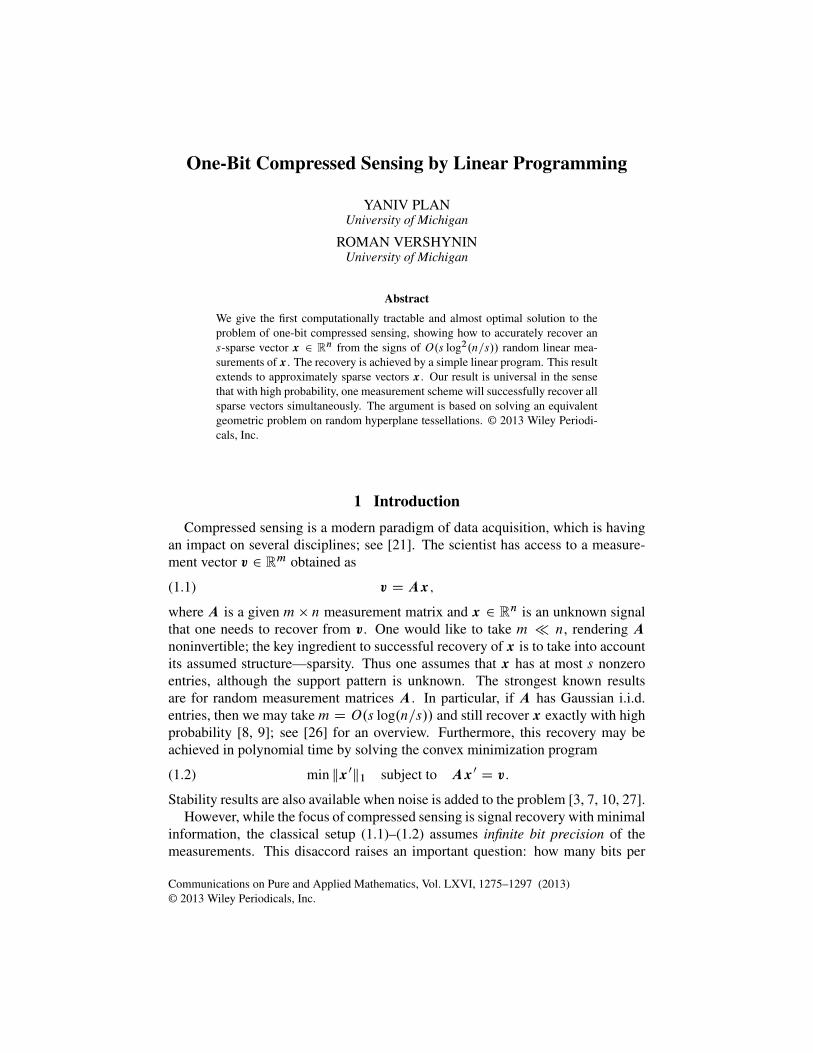
4 Random Hyperplane TessellationsIn this section we prove a generalization of Theorem 2.1. We consider a setK �
Rn and a collection of m random hyperplanes in Rn, chosen independently anduniformly from the Haar measure. The resulting partition of K by this collectionof hyperplanes is called a random tessellation of K. The cells of the tessellationare formed by the intersection of K and the m random half-spaces with particularorientations. The main interest in the theory of random tessellations is the typicalshape of the cells.
We shall study the situation where K is a subset of the sphere Sn�1; see Fig-ure 4.1. The particular example of K D Sn�1 is a natural model of random hyper-plane tessellation in the spherical space Sn�1. The more classical and well-studiedmodel of random hyperplane tessellation is in euclidean space Rn, where the hy-perplanes are allowed to be affine; see [23] for the history of this field. The randomhyperplane tessellations of the sphere is studied in particular in [22].
1-BIT CS BY LINEAR PROGRAMMING 1285
Here we focus on the following question: How many random hyperplanes en-sure that all the cells of the tessellation of K have small diameter (such as 1
2)? For
the purposes of this paper, we shall address this problem for a specific set, namelyfor
K D Sn�1 \psBn1 D Sn�1 \Kn;s:
We shall prove that m D O.s log.n=s// hyperplanes suffice with high probability.Our argument can be extended to more general setsK, but we defer generalizationsto a later paper.
THEOREM 4.1 (Random Hyperplane Tessellations). Let s � n and m be positiveintegers. Consider the tessellation of the set K D Sn�1 \
psBn1 by m random
hyperplanes in Rn chosen independently and uniformly from the Haar measure.Let ı 2 .0; 1/, and assume that
m � Cı�5s log.2n=s/:
Then, with probability at least 1 � 2 exp.�ım/, all cells of the tessellation of Khave diameter at most ı.
It is convenient to represent the random hyperplanes in Theorem 4.1 as .ai /?,i D 1; : : : ; m, where ai are i.i.d. standard normal vectors in Rn. The claim thatall cells of the tessellation of K have diameter at most ı can be restated in thefollowing way: Every pair of points x;y 2 K satisfying kx�yk2 > ı is separatedby at least one of the hyperplanes, so there exists i 2 Œm� such that
hai ;xi > 0; hai ;yi < 0:
Theorem 4.1 is then a direct consequence of the following slightly stronger result:
THEOREM 4.2 (Separation by a Set of Hyperplanes). Let s � n and m be positiveintegers. Consider the set K D Sn�1 \
psBn1 and independent random vectors
a1; : : : ; am � N .0; Id/ in Rn. Let ı 2 .0; 1/, and assume that
m � Cı�5s log.2n=s/:
Then, with probability at least 1�2 exp.�ım/, the following holds: For every pairof points x;y 2 K satisfying kx � yk2 > ı, there is a set of at least cım of theindices i 2 Œm� that satisfy
hai ;xi > cı; hai ;yi < �cı:
We will prove Theorem 4.2 by the following covering argument, which willallow us to uniformly handle all pairs x;y 2 K satisfying kx � yk2 > ı. Wechoose an "-net N" ofK as in Lemma 3.4. We decompose the vector x D x0Cx0
where x0 2 N" is a “center” and x0 2 "Bn2 \ K is a “tail,” and we do similarlyfor y . An elementary probabilistic argument and a union bound will allow us tonicely separate each pair of centers x0;y0 2 N" satisfying kx0 � y0k2 > ı by�.m/ hyperplanes. (Specifically, it will follow that hai ;x0i > cı, hai ;y0i < �cıfor at least cım of the indices i 2 Œm�.)
1286 Y. PLAN AND R. VERSHYNIN
Furthermore, the tails x0;y 0 2 "Bn2 \psBn1 can be uniformly controlled using
Lemma A.2, which implies that all tails are in a good position with respect tom � o.m/ hyperplanes. (Specifically, for small " one can deduce that jhai ;x0ij <cı=2, jhai ;y 0ij < cı=2 for at least m� cım=2 of the indices i 2 Œm�.) Putting thecenters and the tails together, we shall conclude that x and y are separated at least�.m/Cm � o.m/ > �.m/ hyperplanes, as required.
Now we present the full proof of Theorem 4.2.
4.1 Step 1: Decomposition into Centers and TailsLet " 2 .0; 1/ be a number to be determined later. Let N" be an "-net of K.
Since K � Kn;s , Lemma 3.4 along with the monotonicity property of entropy(3.2) guarantee that N" can be chosen so that
(4.1) log jN"j �Cs
"2log
�2n
s
�:
LEMMA 4.3 (Decomposition into Centers and Tails). Let t D 4s="2. Then everyvector x 2 K can be represented as
(4.2) x D x0 C "x0
where x0 2 N", x0 2 Kn;t .
PROOF. Since N" is an "-net ofK, representation (4.2) holds for some x0 2 Bn2 .Since Kn;t D Bn2 \
ptBn1 , it remains to check that x0 2
ptBn1 . Note that x 2
K �psBn1 and x0 2 N" � K �
psBn1 . By the triangle inequality, this implies
that "x0 D x � x0 2 2psBn1 . Thus x0 2 .2
ps="/Bn1 D
ptBn1 , as claimed. �
4.2 Step 2: Separation of the CentersOur next task is to separate the centers x0, y0 of each pair of points x;y 2 K
that are far apart by �.m/ hyperplanes. For a fixed pair of points and for onehyperplane, it is easy to estimate the probability of a nice separation.
LEMMA 4.4 (Separation by One Hyperplane). Let x;y 2 Sn�1 and assume thatkx � yk2 � ı for some ı > 0. Let a � N .0; Id/. Then for ı0 D ı=12 we have
Pfha;xi > ı0; ha;yi < �ı0g � ı0:
PROOF. Note that
Pfha;xi > ı0; ha;yi < �ı0g
D Pfha;xi > 0 and ha;yi < 0 and ha;xi … .0; ı0� and ha;yi … Œ�ı0; 0/g
The inequality above follows by the union bound. Now, since ha;xi � N .0; 1/we have
Pfha;xi 2 .0; ı0�g �ı0p2�
and Pfha;yi 2 Œ�ı0; 0/g �ı0p2�:
1-BIT CS BY LINEAR PROGRAMMING 1287
Also, denoting the geodesic distance in Sn�1 by d. � ; � / it is not hard to show that
Pfha;xi � 0 or ha;yi � 0g D 1 �d.x;y/
2�� 1 �
kx � yk2
2�� 1 �
ı
2�
(see [13, lemma 3.2]). Thus
Pfha;xi > ı0; ha;yi < �ı0g �ı
2��2ı0p2�� ı0
as claimed. �
Now we will pay attention to the number of hyperplanes that nicely separates agiven pair of points.
DEFINITION 4.5 (Separating Set). Let ı0 2 .0; 1/. The separating index set of apair of points x;y 2 Sn�1 is defined as
Iı0.x;y/ WD fi 2 Œm� W hai ;xi > ı0; hai ;yi < �ı0g:
The cardinality jIı0.x;y/j is a binomial random variable, which is the sum ofm
indicator functions of the independent events fhai ;xi > ı0; hai ;yi < �ı0g. Theprobability of each such event can be estimated using Lemma 4.4. Indeed, supposekx � yk2 � ı for some ı > 0, and let ı0 D ı=12. Then the probability of each ofthe events above is at least ı0. Then jIı0
.x;y/j � Binomial.m; p/ with p > ı0.A standard deviation inequality (e.g., [1, theorem A.1.13]) yields
(4.3) PfjIı0.x;y/j < ı0m=2g � e
�ı0m=8:
Now we take a union bound over pairs of centers in the net N" that was chosenin the beginning of Section 4.1.
LEMMA 4.6 (Separation of the Centers). Let "; ı 2 .0; 1/, and let N" be an "-netof K whose cardinality satisfies (4.1). Assume that
(4.4) m �C1s
"2ılog
�2n
s
�:
Then, with probability at least 1 � exp.�ım=100/, the following event holds:
(4.5)For every x0;y0 2 N" such that kx0�y0k2 > ı,one has jIı=12.x0;y0/j � ım=24.
PROOF. For a fixed pair x0;y0 as above, we can rewrite (4.3) as
PfjIı=12.x0;y0/j < ım=24g � e�ım=96:
A union bound over all pairs x0;y0 implies that the event in (4.5) fails with prob-ability at most
jN"j2 � e�ım=96:By (4.1) and (4.4), this quantity is further bounded by
exp�Cs
"2log
�2n
s
��ım
96
�� exp.�ım=100/
1288 Y. PLAN AND R. VERSHYNIN
provided the absolute constant C1 is chosen sufficiently large. The proof is com-plete. �
4.3 Step 3: Control of the TailsNow we provide a uniform control of the tails x0 2 Kn;t that arise from the
decomposition given in Lemma 4.3. The next result is a direct consequence ofLemma A.2.
LEMMA 4.7 (Control of the Tails). Let t � 1 and let a1; : : : ; am � N .0; Id/ beindependent random vectors in Rn. Assume that
(4.6) m � Ct log.2n=t/:
Then, with probability at least 1 � 2 exp.�cm/, the following event holds:
supx02Kn;t
1
m
mXiD1
jhai ;x0ij � 1:
4.4 Step 4: Putting the Centers and Tails TogetherLet " D c0ı
2 for a sufficiently small absolute constant c0 > 0. To control thetails, we choose an "-net N" of K as in Lemma 4.6, and we shall apply this lemmawith ı=2 instead of ı. Note that requirement (4.4) becomes
m � C2ı�5s log
�2n
s
�;
and it is satisfied by the assumption of Theorem 4.2 for a sufficiently large absoluteconstant C . So Lemma 4.6 yields that with probability at least 1�exp.�ım=200/,the following separation of centers holds:
(4.7)For every x0;y0 2 N" such that kx0 � y0k2 >
ı=2, one has jIı=24.x0;y0/j � ım=48.
To control the tails, we choose t D 4s="2 � s=ı4 as in the decompositionlemma, Lemma 4.3, and we shall apply Lemma 4.7. Note that requirement (4.6)becomes
m � C3ı�4s log
�C3n
s
�;
and it is satisfied by the assumption of Theorem 4.2 for a sufficiently large absoluteconstant C . So Lemma 4.7 yields that with probability at least 1 � 2 exp.�cm/,the following control of tails holds:
(4.8) For every x0 2 Kn;t ; one has1
m
mXiD1
jhai ;x0ij � 1:
Now we combine the centers and tails. With probability at least 1�2 exp.�cım/,both events (4.7) and (4.8) hold. Suppose both these events indeed hold, and con-sider a pair of vectors x;y 2 K as in the assumption, so kx � yk2 > ı. We
1-BIT CS BY LINEAR PROGRAMMING 1289
decompose these vectors according to Lemma 4.3:
(4.9) x D x0 C "x0; y D y0 C "y
0;
where x0;y0 2 N" and x0;y 0 2 Kn;t . By the triangle inequality and the choiceof ", the centers are far apart:
kx0 � y0k2 � kx � yk2 � 2" > ı � 2" D ı � 2c0ı2�ı
2:
Then event (4.7) implies that the separating set
(4.10) I0 WD Iı=24.x;y/ satisfies jI0j �ım
48:
Furthermore, using (4.8) for the tails x0 and y 0 we see that
1
m
mXiD1
jhai ;x0ij C
1
m
mXiD1
jhai ;y0ij � 2:
By Markov’s inequality, the set
I 0 WD
�i 2 Œm� W jhai ;x
0ij C jhai ;y
0ij �
192
ı
�satisfies j.I 0/cj �
ım
96:
We claim that
I WD I0 \ I0
is a set of indices i that satisfies the conclusion of Theorem 4.2. Indeed, the numberof indices in I is as required since
jI j � jI0j � j.I0/cj �
ım
48�ım
96Dım
96:
Further, let us fix i 2 I . Using decomposition (4.9) we can write
hai ;xi D hai ;x0i C "hai ;x0i:
Since i 2 I � I0 D Iı=24.x;y/, we have hai ;x0i > ı=24, while from i 2 I � I 0
we obtain hai ;x0i � �192=ı. Thus
hai ;xi >ı
24�192"
ı�ı
30;
where the last estimate follows by the choice of " D c0ı2 for a sufficiently small
absolute constant c0 > 0. In a similar way one can show that
hai ;yi < �ı
24C192"
ı� �
ı
30:
This completes the proof of Theorem 4.2. �
1290 Y. PLAN AND R. VERSHYNIN
5 Effective Sparsity of SolutionsIn this section we prove Theorem 2.4 about the effective sparsity of the solution
of the convex optimization problem (1.3). Our proof consists of two steps: a lowerbound for kyxk2 proved in Lemma 5.1 below, and an upper bound on kxk2, whichwe can deduce from Lemma A.2 in the Appendix.
LEMMA 5.1 (Euclidean Norm of Solutions). Let n;m > 0. Then, with probabil-ity at least 1 � C exp.�cm log.2n=m C 2m=n//, the following holds uniformlyfor all signals x 2 Rn: Let y D sign.Ax/. Then the solution yx of the convexminimization program (1.3) satisfies
kyxk2 �cp
log.2n=mC 2m=n/:
Remark 5.2. Note that the sparsity of the signal x plays no role in Lemma 5.1; theresult holds uniformly for all signals x.
Let us assume that Lemma 5.1 is true for a moment and show how together withLemma A.2 it implies Theorem 2.4.
PROOF OF THEOREM 2.4. With probability at least 1 � C exp.�cm/, the con-clusions of both Lemma 5.1 and Lemma A.2 with t D 1
4hold. Assume this event
occurs. Consider a signal x as in Theorem 2.4 and the corresponding solution yx of(1.3). By Lemma 5.1, the latter satisfies
(5.1) kyxk2 �cp
log.2n=mC 2m=n/:
Next, consider
� D1
m
mXiD1
jhai ;xij D1
mkAxk1:
Since by the assumption on x we have x=kxk2 2 Kn;s \ Sn�1, Lemma A.2 witht D 1
4implies that
(5.2) � �kxk2
2:
By definition of �, the vector ��1x is feasible for the program (1.3), so the solu-tion yx of this program satisfies
kyxk1 � k��1xk1 D �
�1kxk1:
Putting this together with (5.2) and (5.1), we conclude that
kyxk1
kyxk2�kxk1
�kyxk2�
2kxk1
kxk2kyxk2�kxk1
kxk2� Cp
log.2n=mC 2m=n/:
This completes the proof of Theorem 2.4. �
1-BIT CS BY LINEAR PROGRAMMING 1291
In the rest of this section we prove Lemma 5.1. The argument is based on theobservation that the set of possible solutions yx of the convex program (1.3) forall x and corresponding y is finite, and its cardinality can be bounded by the valueexp.Cm log.2n=mC 2m=n//. For each fixed solution yx, a lower bound on kyxk2will be deduced from Gaussian concentration inequalities, and the argument willbe finished by taking a union bound over yx.
It may be convenient to recast the convex minimization program (1.3) as a linearprogram by introducing the dummy variables u D .u1; : : : ; un/:
(5.3) minnXiD1
ui such that
8<:�ui � x
0i � ui ; i D 1; : : : ; nI
yi hai ;x0i � 0; i D 1; : : : ; mI
1m
PmiD1 yi hai ;x
0i � 1:
The feasible set of the linear program (5.3) is a polytope in R2n, and the lin-ear program attains a solution on a vertex of this polytope. Further, since ai arecontinuous random vectors, one can check that the solution of the linear programis unique with probability 1. Thus, by characterizing these vertices and pointingout the relationship between ui and yxi , we may reduce the space of possible so-lutions yx. This is the content of our next lemma. Given subsets T � f1; : : : ; ng,� � f1; : : : ; mg, we define A�
T to be the submatrix of A with columns indexed byT and rows indexed by �.
LEMMA 5.3 (Vertices of the Feasible Polytope). With probability 1, the linearprogram (5.3) attains a solution .yx;u/ at a point that satisfies the following forsome T � f1; : : : ; ng and � � f1; : : : ; mg:
(1) ui D jyxi j,(2) supp.yx/ D T ,(3) jT j D j�j C 1,(4) A�
T yxT D 0,(5) 1
m
PmiD1jhai ; yxij D 1.
PROOF. Part (1) follows since we are minimizingPui . Part (5) follows since
1
m
mXiD1
yi hai ; yxi D1
m
mXiD1
jhai ; yxij
combined with the fact that we are implicitly minimizing kx0k1. Parts (2) through(4) will follow from the fact that (5.3) achieves its minimum at a vertex. Thevertices are precisely the feasible points for which some d of the inequality con-straints achieve equality, provided yx is the unique solution to those d equalities.Since .yx;u/ 2 R2n, at least 2n of the constraints must be equalities. We now countequalities based on T and �.
We first consider the constraints �ui � x0i � ui , i D 1; : : : ; n. If yxi D 0 wehave two equalities, �ui D yxi and ui D yxi ; otherwise, we have one. This givesnC jT cj equalities.
1292 Y. PLAN AND R. VERSHYNIN
Part (5) gives one more equality. This leaves us with at least 2n�n�jT cj�1 D
jT j � 1 equalities that must be satisfied out of the equations yi hai ; yxi � 0. Thus,we may take j�j D jT j � 1. �
PROOF OF LEMMA 5.1. We may disregard the dummy variables .ui / and con-sider that the solution yx D x0 must satisfy conditions (2) through (5) above forsome T and �. We will show that with high probability, any such vector x0 2 Rn
is lower bounded in the euclidean norm.Let us first fix sets T and �, and consider a vector x0 satisfying (2) through (5).
We represent it as
x0 D �xx for some � > 0 and kxxk2 D 1:
Our goal is to lower bound �. By condition (4) above, we have A�T xxT D 0, which,
with probability 1, completely determines the vector xx up to multiplication by ˙1(since jT j D j�j C 1 and xxT c D 0). Moreover, since supp.xx/ D supp.x0/ D T ,we have 0 D A�
T xxT D A�xx, so hai ;x0i D 0 for i 2 �. Using this together withcondition (5), we obtain
1 D �1
m
mXiD1
jhai ; xxij D �1
m
Xi…�
jhai ; xxij
and thus
(5.4) kx0k2 D � D
�1
m
Xi…�
jhai ; xxij
��1:
We proceed to upper bound 1m
Pi…�jhai ; xxij.
Since the random vector xx depends entirely on A�T , it is independent of ai for
i … �. Thus, by the rotational invariance of the Gaussian distribution, for any fixedvector ´ with unit norm, we have the following distributional estimates:2
1
m
Xi…�
jhai ; xxijdistD
1
m
Xi…�
jhai ; ´ijdist�
1
m
mXiD1
jhai ; ´ij:
The last term is a sum of independent sub-Gaussian random variables, and it canbe bounded using standard concentration inequalities. Specifically, applying Lem-ma A.1 from the Appendix, we obtain
P
�1
m
mXiD1
jhai ; ´ij > t
�� C exp.�cmt2/ for t � 2:
Using (5.4), this is equivalent to
Pfkx0k2 < 1=tg � C exp.�cmt2/ for t � 2:
2 For random variables X and Y , the distributional inequality Xdist� Y means that PfX > tg �
PfY > tg for all t 2 R.
1-BIT CS BY LINEAR PROGRAMMING 1293
It is left to upper bound the number of vectors satisfying conditions (2) through (5)and to use the union bound. Since jT j D j�j C 1, the total number of possiblechoices for T and � (and hence of x0) is
min.m;n�1/XiD0
�n
i C 1
��m
i
�� exp.Cm log.2n=mC 2m=n//:
Thus, by picking t D C0p
log.2n=mC 2m=n/ with a sufficiently large absoluteconstant C0, we find that all x0 uniformly satisfy the required estimate
kx0k2 �cp
log.2n=mC 2m=n/
with probability at least 1 � exp.Cm log.2n=m C 2m=n// � C exp.�cmt2/ D1 � C exp.�cm log.2n=mC 2m=n//. Lemma 5.1 is proved. �
Appendix: Uniform Concentration InequalityIn this section we prove concentration inequalities for
kAxk1 D
mXiD1
jhai ;xij:
In the situation where the vector x is fixed, we have a sum of independent randomvariables, which can be controlled by standard concentration inequalities:
LEMMA A.1 (Concentration). Let n;m 2 N and x 2 Rn. Then, for every t > 0
one has
P
�ˇ1
m
mXiD1
jhai ;xij �
r2
�kxk2
ˇ> tkxk2
�� C exp.�cmt2/:
PROOF. Without loss of generality we can assume that kxk2 D 1. Then hai ;xiare independent standard normal random variables, so Ejhai ;xij D
p2=� . There-
fore Xi WD jhai ;xij �p2=� are independent and identically distributed cen-
tered random variables. Moreover, the Xi are sub-Gaussian random variables withkXik 2
� C ; see [26, remark 18]. An application of a Hoeffding-type inequality(see [26, proposition 10]) yields
P
�ˇ1
m
mXiD1
Xi
ˇ> t
�� C exp.�cmt2/:
This completes the proof. �
We will now prove a stronger version of Lemma A.1 that is uniform over alleffectively sparse signals x.
1294 Y. PLAN AND R. VERSHYNIN
LEMMA A.2 (Uniform Concentration). Let n 2 N, t 2 Œ0;p2=��, and suppose
that m � Ct�4s log.2n=s/. Then
P
�sup
x2Kn;s\Sn�1
ˇ1
m
mXiD1
jhai ;xij �
r2
�
ˇ> t
�� C exp.�cmt2/:
PROOF. This is a standard covering argument, although the approximation steprequires a little extra care. Let M be a t=4-net of Kn;s \ Sn�1. Since Kn;s \Sn�1 � Kn;s , we can arrange by Lemma 3.4 that
jMj � exp.C t�2s log.2n=s//:
By definition, for any x 2 Kn;s \Sn�1 one can find xx 2M such that kx� xxk2 �t=4. So the triangle inequality yieldsˇ
1
m
mXiD1
jhai ;xij �
r2
�
ˇ�
ˇ1
m
mXiD1
jhai ; xxij �
r2
�
ˇC1
m
mXiD1
jhai ;x � xxij:
Note that kx � xxk1 � kxk1 C kxxk1 � 2ps. Together with kx � xxk2 � t=4 this
means that
x � xx 2t
4�Kn;64s=t2 :
Consequently,
supx2Kn;s\Sn�1
�1
m
mXiD1
jhai ;xij �
r2
�
�
� supxx2M
ˇ1
m
mXiD1
jhai ; xxij �
r2
�
ˇCt
4� sup
w2Kn;64s=t2
1
m
mXiD1
jhai ;wij
DW R1 Ct
4�R2:
(A.1)
We bound the terms R1 and R2 separately. For simplicity of notation, we assumethat 64s=t2 is an integer, as the noninteger case will have no significant effect onthe result.
A bound on R1 follows from the concentration estimate in Lemma A.1 and aunion bound:
PfR1 > t=4g � jMj � C exp.�cmt2/
� C exp.C t�2s log.2n=s/ � cmt2/
� C exp.�cmt2/
(A.2)
provided that m � Ct�4s log.2n=s/.
1-BIT CS BY LINEAR PROGRAMMING 1295
Next, due to Lemma 3.1 and Jensen’s inequality, we have
R2 � 2 supw2S
n;64s=t2
1
m
mXiD1
jhai ;wij
� 2 supw2S
n;64s=t2
�1
m
mXiD1
hai ;wi2
�1=2DW 2R02:
The quantity R02 has been well studied in compressed sensing; it is bounded bythe restricted isometry constant of the matrix .1=
pm/A at sparsity level 64s=t2.
Probabilistic bounds for the restricted isometry constants of Gaussian matrices arewell known and have been derived in the earliest compressed sensing works [9].We use the bound in [26, theorem 65] that gives
(A.3) PfR02 > 1:5g � 2 exp.�cm/
provided that m � Ct�2s log.n=s/. Thus
PfR2 > 3g � 2 exp.�cm/:
Combining this and (A.2) we conclude that
P
�R1 C
t
4�R2 > t
�� C 0 exp.�cmt2/
where we used the assumption that t �p2=� . This and (A.1) complete the
proof. �
Acknowledgment. The authors are grateful to Sinan Güntürk for pointing outan inaccuracy in the statement of Lemma 3.4 in an earlier version of this paper.
Bibliography[1] Alon, N.; Spencer, J. H. The probabilistic method. Second edition. Wiley-Interscience Series in
Discrete Mathematics and Optimization. Wiley-Interscience, New York, 2000.[2] Ardestanizadeh, E.; Cheraghchi, M.; Shokrollahi, A. Bit precision analysis for compressed
sensing. Proceedings of the 2009 IEEE International Conference on Symposium on InformationTheory, vol. 1, 1–5. Piscataway, N.J., IEEE Press, 2009 . Available at: http://dl.acm.org/citation.cfm?id=1701495.1701496
[3] Bickel, P. J.; Ritov, Y.; Tsybakov, A. B. Simultaneous analysis of lasso and Dantzig selec-tor. Ann. Statist. 37 (2009), no. 4, 1705–1732. Available at: http://projecteuclid.org/euclid.aos/1245332830.
[4] Boufounos, P. T. Greedy sparse signal reconstruction from sign measurements. 2009 Confer-ence Record of the Forty-Third Asilomar Conference on Signals, Systems and Computers, 1305–1309. doi:10.1109/ACSSC.2009.5469926
[5] Boufounos, P. T. Reconstruction of sparse signals from distorted randomized measurements.2010 IEEE International Conference on Acoustics, Speech and Signal Processing (ICASSP),3998–4001. doi:10.1109/ICASSP.2010.5495766
[6] Boufounos, P. T.; Baraniuk, R. G. 1-bit compressive sensing. In 42nd Annual Conference onInformation Sciences and Systems (CISS), 2008, 16–21. doi:10.1109/CISS.2008.4558487
[7] Candès, E. J.; Romberg, J. K.; Tao, T. Stable signal recovery from incomplete and inaccuratemeasurements. Comm. Pure Appl. Math. 59 (2006), no. 8, 1207–1223. doi:10.1002/cpa.20124
[8] Candes, E.; Rudelson, M.; Vershynin, R.; Tao, T. Error correction via linear program-ming. 46th Annual IEEE Symposium on Foundations of Computer Science, 2005, 668–681.doi:=10.1109/SFCS.2005.5464411
[9] Candes, E. J.; Tao, T. Near-optimal signal recovery from random projections: universal en-coding strategies? IEEE Transactions on Information Theory 52 (2006), no. 12, 5406–5425.doi:10.1109/TIT.2006.885507
[10] Candes, E.; Tao, T. The Dantzig selector: statistical estimation when p is much larger than n.Ann. Statist. 35 (2007), no. 6, 2313–2351. doi:10.1214/009053606000001523
[11] Dai, W.; Pham, H. V.; Milenkovic, O. A comparative study of quantized compressivesensing schemes. IEEE International Symposium on Information Theory, 2009, 11–15.doi:10.1109/ISIT.2009.5206032
[12] Damaschke, P. Threshold group testing. Electronic Notes in Discrete Mathematics 21 (2005),265–271. doi:10.1016/j.endm.2005.07.040
[13] Goemans, M. X.; Williamson, D. P. Improved approximation algorithms for maximum cut andsatisfiability problems using semidefinite programming. J. Assoc. Comput. Mach 42 (1995),no. 6, 1115–1145. doi:10.1145/227683.227684
[14] Güntürk, C.; Lammers, M.; Powell, A.; Saab, R.; Ylmaz, O. Sigma delta quantization for com-pressed sensing. 2010 44th Annual Conference on Information Sciences and Systems (CISS),1–6. doi:10.1109/CISS.2010.5464825
[15] Güntürk, C.; Powell, A.; Saab, R.; Ylmaz, Ö. Sobolev duals for random frames and sigma-deltaquantization of compressed sensing measurements. Preprint, 2010. arXiv:1002.0182 [cs.IT]
[16] Gupta, A.; Nowak, R.; Recht, B. Sample complexity for 1-bit compressed sensing and sparseclassification. 2010 IEEE International Symposium on Information Theory Proceedings (ISIT),1553–1557. doi:10.1109/ISIT.2010.5513510
[17] Jacques, L.; Hammond, D. K.; Fadili, J. M. Dequantizing compressed sensing: when oversam-pling and non-gaussian constraints combine. IEEE Trans. Inform. Theory 57 (2011), no. 1,559–571.
[18] Jacques, L.; Laska, J. N.; Boufounos, P. T.; Baraniuk, R. G. Robust 1-bit compressive sensingvia binary stable embeddings of sparse vectors. Preprint, 2011. arXiv:1104.3160 [cs.IT]
[19] Laska, J. N.; Boufounos, P. T.; Davenport, M. A.; Baraniuk, R. G. Democracy in action: quan-tization, saturation, and compressive sensing. Appl. Comput. Harmon. Anal. 31 (2011), no. 3,429–443. doi:10.1016/j.acha.2011.02.002
[20] Laska, J. N.; Wen, Z.; Yin, W.; Baraniuk, R. G. Trust, but verify: fast and accurate signalrecovery from 1-bit compressive measurements. IEEE Trans. Signal Process. 59, no. 11, 5289–5301.
[21] Mackenzie, D. Compressed sensing makes every pixel count. What’s Happening in the Mathe-matical Sciences (2009), no. 7, 114–127.
[22] Miles, R. E. Random points, sets and tessellations on the surface of a sphere. Sankhya Ser. A 33(1971), 145–174.
[23] Møller, J.; Stoyan, D. Stochastic geometry and random tessellations. In Tessellations in thesciences: virtues, techniques and applications of geometric tilings, to appear.
[24] Pisier, G. The volume of convex bodies and Banach space geometry. Cambridge Tracts in Math-ematics, 94. Cambridge University Press, Cambridge, 1989.
[25] Sun, J.; Goyal, V. Optimal quantization of random measurements in compressed sensing. IEEEInternational Symposium on Information Theory, 2009, 6–10. doi:10.1109/ISIT.2009.5205695
[26] Vershynin, R. Introduction to the non-asymptotic analysis of random matrices. Compressedsensing: theory and applications, 210–268. Cambridge University Press, Cambridge, 2012.
[27] Wojtaszczyk, P. Stability and instance optimality for Gaussian measurements in compressedsensing. Found. Comput. Math. 10 (2010), no. 1, 1–13. doi:10.1007/s10208-009-9046-4