arX

iv:0

710.

0850

v1 [

mat

h.PR

] 3

Oct

200

7

Monte Carlo Methods and Path-Generation

techniques for Pricing Multi-asset Path-dependent

Options

Piergiacomo SabinoDipartimento di MatematicaUniversita degli Studi di Bari

sabino@dm.uniba.itReport 36/07

Abstract

We consider the problem of pricing path-dependent options on a basket of underlyingassets using simulations. As an example we develop our studies using Asian options.

Asian options are derivative contracts in which the underlying variable is the averageprice of given assets sampled over a period of time. Due to this structure, Asian op-tions display a lower volatility and are therefore cheaper than their standard Europeancounterparts.

This paper is a survey of some recent enhancements to improve efficiency whenpricing Asian options by Monte Carlo simulation in the Black-Scholes model. Weanalyze the dynamics with constant and time-dependent volatilities of the underlyingasset returns.

We present a comparison between the precision of the standard Monte Carlo method(MC) and the stratified Latin Hypercube Sampling (LHS). In particular, we discuss theuse of low-discrepancy sequences, also known as Quasi-Monte Carlo method (QMC),and a randomized version of these sequences, known as Randomized Quasi Monte Carlo(RQMC). The latter has proven to be a useful variance reduction technique for bothproblems of up to 20 dimensions and for very high dimensions.

Moreover, we present and test a new path generation approach based on a Kroneckerproduct approximation (KPA) in the case of time-dependent volatilities. KPA provesto be a fast generation technique and reduces the computational cost of the simulationprocedure.

Key Words: Monte Carlo and Quasi-Monte Carlo simulations. Effective dimensions.Path-generation techniques. Path-dependent options.

1 Introduction

The financial industry has developed a variety of derivative contracts in order to fulfildifferent investor needs. Path-dependent options play a fundamental role in financialengineering and can display different exotic features.

Exotic contracts that are widely used are Asian options, barrier options and look-back options both with American and European style. An un-biased and efficientpricing procedure is fundamental and a vast research is done in order to obtain fastand efficient estimations. Common approaches rely on finite differences methods andMonte Carlo simulations.

Finite differences methods consist in discretizing the partial differential equationwhose solution gives the price of the options while Monte Carlo methods face the

problem from a probabilistic point of view. It estimates the price as an expected valueby its integral formulation.

The former method returns the fair price of the option for different times and val-ues of the underlying variable but is practically unfeasible for complicated multi-assetdependence.

On the other hand, Monte Carlo simulation calculates the fair price in a single timepoint and can be applied to various situations.

Its fundamental property is that its order of convergence is O(1/√

n) and does notdepend on the number of random sources of the problem. Although it does not display ahigh order of convergence, it proves to be efficient for pricing complex exotic contracts.

The aim of this report is to describe standard and advanced Monte Carlo techniquesapplied for multi-asset Asian options of European style. In particular we concentrateour studies to stratification and Quasi-Monte Carlo approaches.

Standard Monte Carlo can be seen as a numerical procedure aimed to estimateintegrals in the hypercube [0, 1]d by generating different scenarios with uniform randomvariables. Stratification achieves the same task by drawing uniform random variates ina smaller set in [0, 1]d introducing correlation.

Quasi-Monte Carlo methods drop off all probabilistic considerations and focus onthe problem of generating a sequence of points that uniformly covers the hypercube[0, 1)d (the theory is built-up for right-opened intervals). The sequence is absolutelydeterministic and different drawings lead to the same points.

From the mathematical point of view, it introduces the concept of discrepancy andstar-discrepancy that quantify how well the sequences cover [0, 1)d.

Hawkla and Koksma proved the fundamental inequality, named after them, thatprovides the bound for the estimation error of the target integral depending on thediscrepancy.

Low-discrepancy sequences are those whose estimation error is O( lndnn ). The con-

vergence rate depends on the dimension d and is lower than the Monte Carlo error forsmall d. There exist several low discrepancy sequences, among them are the Halton,the Faure, the Sobol and the Niederreiter-Xing sequences. A fundamental reference onthis topic is Niederreiter [17].

Quasi-Monte Carlo methods can be unpractical because the computation of theerror is potentially more difficult than the estimation of the target integral while thebetter uniformity can be lost even for low values of d.

Standard Monte Carlo, stratification and Quasi-Monte Carlo methods form a hier-archy for the generation of uniform points.

A further step ahead can be taken by randomizing these sequences while preserv-ing the low-discrepancy. This technique is called scrambling, Owen [21] provides anextensive description on the subject.

The application to options pricing is straightforward. Standard models for pricedynamics involve multidimensional Ito processes so that pricing exotic contracts mightrequire a high-dimensional integration. It necessitates careful implementation of thesimulation especially when Quasi-Monte Carlo methods are used.

Many works have been done to investigate the problem. Acworth, Broadie, andGlasserman [1] provided a first comparisons between variance reduction techniques andQuasi-Monte Carlo methods and Caflisch, Morokoff and Owen [4] analyzed the effec-tive dimension of the integration problem for mortgage-backed securities by ANOVAconsiderations. Caflisch, Morokoff and Owen [4] and Owen [19] showed that only fewrandom sources really matter and suggested to choose for them a better generationtechnique.

We focus our investigation on pricing Asian options in a multi-dimensional Black-Scholes model both for constant and time-dependent volatilities. In this framework,standard path-generating techniques are the Cholesky decomposition, the principalcomponent analysis (PCA) and linear transform LT. The last two have been provento be essential for ANOVA in order to recognize effective dimensions so that an efficientRQMC can be run.

2

When constant volatilities are considered, the path-generation procedure can besimplified relying on the properties on the Kronecker product while this is not possiblefor time-depending volatilities.

As for this task, we propose a new approach based on a Kronecker product approxi-mation. The general problem consists in approximating the global correlation matrix ofthe price returns into the Kronecker product of two smaller matrices. We assume thatthe former of the two is the auto-covariance matrix of a single brownian motion. Indeed,we suppose that most of the variance of the global process is carried out by each drivingbrownian motion. The latter matrix would be an approximation of the total covariancematrix among the asset returns during the lifetime of the contract. The original andtarget path is reobtained by Cholesky decomposition. As for this last step we developan ad hoc realization of the Cholesky decomposition suited for the global correlationmatrix. This procedure is intended to reduce the computational burden required toevaluate the whole set of eigenvalues and eigenvectors of the global covariance matrix.

The last step of the simulation is the computation of the Asian price via simulationusing standard Monte Carlo, LHS and RQMC approaches. As for the last one weperform a Faure-Tezuka scrabling version of the Sobol’ sequence, which is the mostused low discrepancy sequence in finance.

In the case of constant volatility, we set our investigation as in Dahl and Benth [6],[7] and Imai and Tan [11]. We compare our results and analyze the precision of thesimulation for different path-generation methods and Monte Carlo approach.

As for the time-dependent volatility market we test the KPA method and compareits results with those obtained with the PCA decomposition.

Summarizing the report evolves as follows: section 2 introduces the market. Section3 describes the pay-off of Asian options and presents the problem as an integral for-mulation. Section 4 defines effective dimensions in truncation and superposition sense.Section 5 defines the Kronecker product and list some of the main properties. Section6 describes some path-generation procedures and in particular, it introduces the KPAmethod. Section 7 is a brief introduction to low-discrepancy sequences and scramblingtechniques. Section 8 describes the simulation procedure we adopt. Section 9 showsand comments the estimated results for different scenarios both in the constant andtime-dependent cases.

2 The Market

We consider a complete, standard financial market M in a Black-Scholes framework,with constant risk-free rate r and time-dependent volatilities. There are M + 1 assetsin the market, one risk free asset and M risky assets. The price processes of the assetsin this market are driven by a set of stochastic differential equations.

Suppose we have already applied the Girsanov theorem and found the (unique) risk-neutral probability, the model for the risky assets is the so called multi-dimensionalgeometric brownian motion:

S0(t) = ert (1)

dSi (t) = rSi (t) dt + σi (t)Si (t) dWi (t) , i = 1, . . . , M. (2)

Here Si (t) denotes the i-th asset price at time t, σi (t) represents the instantaneous time-dependent volatility of the i-th asset return, r is the continuously compounded risk-freeinterest rate, and W (t) = (W1 (t) , . . . , WM (t)) is an M -dimensional Brownian motion.Time t can vary in R

∗+, that is, we can consider any maturity T ∈ R

∗+ for all financial

contracts.The multi-dimensional brownian motion W (t) is a martingale, that is, each com-

ponent is a martingale, and satisfies the following properties:

E [Wi (t)] = 0, i = 1, . . . , M.

[Wi, Wk] (t) = ρikt, i, k = 1, . . . , M.

3

where [�, �](t) represents the quadratic variation up to time t and ρik the constantinstantaneous correlation between Wi and Wk.

Consider a generic maturity T , we can define a time grid T = {t1, . . . , tN} of Npoints such that t1 < t2 < . . . , tN = T , we recall that the sampled covariance matrixRl,m = E [Wi (tl)Wi (tm)], l, m = 1, . . . , N of each Brownian motion in equation (2) is:

R =

t1 t1 . . . t1t1 t2 . . . t2...

.... . .

...t1 t2 . . . tN

. (3)

This matrix is symmetric and its elements Rl,m = tl ∧ tm have the peculiarity to beconstant after reflection about the diagonal. We will refer to this feature as boomerangshape property.

In order to complete the picture of our environment, we need to define the matrixΣ(t), whose elements are Σi,k(t) =ρikσi(t)σk(t), i, k = 1, . . . M . This is a time de-pendent covariance matrix evolving according to the dynamics of the time-dependentvolatilities and the constant correlation among the asset returns.

Avoiding all the calculation (see Rebonato [24] and Glassermann [8] for furtherdetails), we derive the global covariance matrix ΣMN that assumes the expression below:

ΣMN =

Σ(t1) Σ(t1) . . . Σ(t1)Σ(t1) Σ(t2) . . . Σ(t2)

......

. . ....

Σ(t1) Σ(t2) . . . Σ(tN )

(4)

The global covariance matrix is very simple and enjoys the boomerang shape propertywith respect to the block-matrix notation. All the information is carried out by Ntime-varying M × M matrices.

Each element depends on four indexes:

((ΣMN

)ik

)

lm=

∫ tl∧tm

0

σi(t)σk(t)ρikdt (5)

with i, k = 1, . . . , M and l, m = 1, . . . , N .Applying the risk-neutral pricing formula, the value at time t of any European

T -maturing derivative contract is:

V (t) = exp (r(T − t)) E [φ(T )| Ft]. (6)

E denotes the expectation under the risk neutral probability measure and φ(T ) is ageneric FT measurable function, with FT = σ{0 < t ≤ T ; W (t)}, that determines thepayoff of the contract. Although not explicitly written, the function φ(T ) depends onthe entire multi-dimensional brownian path up to time T .

3 Problem Settlement

We will restrict our analysis to Asian options that are exotic derivative contracts thatcan be written both on a single security and on a basket of underlying securities.Hereafter we will consider European-style Asian options whose underlying securitiescoincide with the M + 1 assets on the market. This is the most general case we cantackle in the market M, because it is complete in the sense that we can hedge anyfinancial instrument by finding a portfolio that is a combination of this M + 1 assets.

3.1 Asian Options Payoff

The theoretical definition of Asian options price is:

ai(t) = exp (r(T − t)) E

(∫ T

0Si(t)dt

T− K

)+ ∣∣∣∣Ft

Option on a Single Asset (7)

4

a(t) = exp (r(T − t)) E

(∫ T

0

∑Mi=1 wiSi(t)dt

T− K

)+ ∣∣∣∣Ft

, Option on a Basket

(8)where we assume that the start date of the contract is t = 0. K represents the strikeprice and coefficients wi satisfy

∑Mi=1 wi = 1. Contingent claims (7) and (8) are usually

referred as weighted Asian options.In practice no contract is agreed according to equations (7) and (8). The integrals

are approximated by sums; often these approximations are written in the contracts byspecifying the number and the sampling points of the path.

Approximation for (7) and (8) can be carried out by using the following expressions:

ai (t) = exp (r(T − t)) E

(∑N

j=1 Si (tj)

N− K

)+ ∣∣∣∣Ft

Option on a Single Asset

(9)

a (t) = exp (r(T − t)) E

M∑

i=1

N∑

j=1

wij Si (tj) − K

+ ∣∣∣∣Ft

Option on a Basket (10)

where coefficients wij satisfy∑

i,j wij = 1.European options with payoff functions (9) and (10) are called arithmetic weighted

average options or simply arithmetic Asian options. When M > 0 and N = 1 thepayoff only depends on the terminal price of the basket of M underlying assets and theoption is known as basket option.

No closed-form solution exists for Asian options arbitrage-free price, neither forsingle nor for basket options both for theoretical and finitely monitored payoff. Inorder to obtain a correct valuation of the price we are compelled to turn to numericalprocedures such as the Monte Carlo estimation or the finite difference methods.

The latter is based on a convenient and correct discretization of the partial differ-ential equation associated to the risk neutral pricing formula via the Feynmann-Kacrepresentation. The finite difference method returns the price for all the times andinitial values of the underlying assets. Vecer [26] and [27] found a convenient approachfor the single asset case and presents the comparison with other techniques. The maindrawback is the stability of the method that is practically unfeasible for options on abasket.

Monte Carlo simulation is a numerically intensive methodology that provides unbi-ased estimates with convergence rate not depending on the dimension of the problem(the number of random sources to draw). The cases of high values for the problem di-mension find interesting applications in finance including the pricing of high-dimensionalmulti-factor path-dependent options. In contrast to the finite difference technique, theMonte Carlo method returns the estimate for a single point in time. It is a flexible ap-proach but requires ad hoc implementation and refinements, such as variance reductiontechniques, in order to improve its efficiency.

The main purpose of the standard Monte Carlo method is to numerically estimatethe integral below:

I =

∫

[0,1]df(x)dx. (11)

The integral I can be regarded as E [f(U)], the expected value of a function f(�) of therandom vector U that is uniformly distributed in hypercube [0, 1]d.

Monte Carlo methods simply estimate I by drawing a sample of n independentreplicates U1 . . . , Un of U and then computing the arithmetic average:

I = In =1

n

n∑

i=1

f(Ui). (12)

The Law of Large Numbers ensures that In converges to I in probability a.s. andthe Central Limit Theorem states that I− In converges in distribution to a normal with

5

mean 0 and standard deviation σ/√

n with σ =√∫ 1

0 (f(x) − I)2dx. The convergence

rate is than O(1/√

n) for all dimensions d. The parameter σ is generally unknown ina setting in which I is unknown, but it can be estimated using the sampled standarddeviation or root mean square error (RMSE):

RMSE =

√√√√ 1

n − 1

n∑

i=1

(f(Ui) − In

)2

. (13)

Refinements in Monte Carlo methods consist in finding techniques whose aim is toreduce the RMSE, known as variance reduction techniques, without changing the con-vergence rate. In contrast, the Quasi Monte Carlo version focuses on the improvementof the convergence rate by generating sequences in [0, 1]d with high stratification inorder to uniformly cover the hypercube. These sequences are no longer random andestimates and errors are not based on probabilistic considerations.

As far as our case is concerned, we need to formulate the problems (9) and (10) forpricing Asian options as integrals of the form (11) in order to apply the Monte Carloprocedure.

3.2 Problem Formulation as an Integral

The model M, presented in the first section, consists of the risk-free money marketaccount and M assets driven M geometric brownian motion described by equation (2)whose solution is:

Si (t) = Si (0) exp

[∫ t

0

(r − σ2

i (s)

2

)ds +

∫ t

0

σi (s) dWi (s)

], i = 1, ..., M. (14)

The quantity∫ T

0σ2

i (s)T ds is the total volatility for the i-th asset. The solution (14) is

a multi-dimensional geometric brownian motion, written GBM(r,∫ t

0σ2

i (s)2 ds

), in the

sense that it can be obtained applying Ito’s lemma to Si(t) = f (Xi(t)) = eXi(t), withXi(t) the i-th component of the multi-dimensional brownian motion with drift r and

i-th diffusion∫ t

0σ2

i (s)2 ds, written BM

(r,∫ t

0σ2

i (s)2 ds

).

Under the assumption of constant volatility the solution is still a multi-dimensionalgeometric brownian motion with the following form:

Si (t) = Si (0) exp

[(r − σ2

i

2

)t + σiWi (t)

], i = 1, ..., M. (15)

In compacted notation the solution (15) is GBM(r,

σ2

i

2

).

Pricing Asian option requires to monitor the solutions (14) and (15) at a finite setof points in time {t1, . . . , tN}. This sampling procedure yields the following expressionsfor time-dependent and constant volatilities:

Si(tj) = Si(0)exp

[∫ tj

0

(r − σ2

i (s)

2

)ds + Zi(tj)

](16)

Si(tj) = Si(0)exp

[(r − σ2

i

2

)ttj

+ Zi(tj)

](17)

where the components of the vector (Z1(t1), . . . Z1(tN ), Z2(t1), . . . , ZM (tN )) are M ×Nnormal random variables with zero mean vector and covariance matrix ΣMN , whoseform simplifies in the case of constant volatilities as we will be shown in Section 4.

The payoff at maturity T of the arithmetic average Asian option is then:

pa(T ) = (g(Z) − K)+

(18)

6

where

g(Z) =

M×N∑

k=1

exp (µk + Zk) (19)

and

µk = ln(wk1k2Sk1

(0)) +

(r −

σ2k1

2

)tk2

(20)

for constant volatilities or

µk = ln(wk1k2Sk1

(0)) + rtk2−∫ tk2

0σ2

k1(s)ds

2(21)

for time-dependent volatilities. The indexes k1 and k2 are k1 = (k − 1)modM, k2 =[(k−1)/M ]+1, respectively, where mod denotes the modulus and [�] the greatest integerless than or equal to x.

The calculation of the price a(t) in equation (10) can be formulated as an integralon R

NM in the following way (see Dahl and Benth [6] and [7]):

a (t) = exp (r(T − t))

∫

RMN

(g(z) − K)+

FZ(dz) (22)

FZ is the cumulative distribution of the normal random vector N(0, ΣNM ).In the following section we will show how to obtain the random vector Z starting

from a vector of independent and normally distributed random variables ǫ. Once thisgeneration is carried out, we can apply the inverse transform method to formulate thepricing problem as an integral of uniform random variables in the hypercube [0, 1]MN

and use Monte Carlo methods:

a (t) = exp (r(T − t))

∫

[0,1]NM

(g(u) − K)+ F−1Z (u)du (23)

In the following sections we will present recent enhancement based on ANOVA forhigh dimensional Monte Carlo and Quasi-Monte Carlo simulations in order to estimatethe integral (23) for the pricing Asian option on a basket of underlying assets both forconstant and time-dependent volatilities.

4 Effective Dimensions

When the nominal dimension d of the problem of estimating the integral (11) is one,there are standard numerical techniques that give a good accuracy when f is smooth.Considerable problems arise when d is high.

Recent studies proved that many financial experiments present problem dimensionslower than the nominal one. Owen (1998) [19] and Caflisch, Morokoff and Owen [4]studied the application of ANOVA for high-dimensional problems and introduced thedefinition of effective dimension. It is possible to study some mathematical propertiesof the function f and try to split it in order to reduce the computational effort. TheANOVA decomposition consists of finding a representation of f into orthogonal func-tions each of them depending only on a subset of the original variables. This is thepeculiar and stronger condition that makes ANOVA different and more powerful withrespect to the usual Least Squared method.

Let A = {1, . . . , d} denote the set of the independent variables for f on [0, 1]d.f could be written into the sum of 2d orthogonal functions each of them defined indifferent subsets of A, that is depending only on the variables in each of these subsets:

f(x) =∑

u⊆Afu(x) (24)

7

Now let |u| denote the cardinality of u, xu the |u|-tuple consisting of components xj

with j ∈ u, and −u being the complement of u in A. Then set the function as:

fu(x) =

∫

z:zu=xu

(f(z) −

∑

v⊂u

fv(z)

)dz−u (25)

Equation (25) defines fu by subtracting what can be attributed to the subsets of u,and then averaging over all components not in u. In the function setting fu(xu) onlydepends on xu.Denoting σ2 =

∫(f(x) − I)2 dx, σ2

u =∫

fu(x)2 dx, σ20 = 0, supposing σ < +∞ and

|u| > 0 it follows:

σ2 =∑

u⊆Aσ2

u (26)

Equation (26) partitions the total variance into parts corresponding to each subset u ⊆A. The fu exhibits some nice properties: if j ∈ u the line integral

∫[0,1] fu(x) dxj = 0

for any xk with k 6= j, and if u 6= v∫

fu(x)fv(x) dx = 0.Exploiting the ANOVA decomposition the definition of effective dimension can be

given in the following ways:

Definition 1. The effective dimension of f , in the superposition sense, is the smallestinteger dS such that

∑0<|u|≤dS

σ2u ≥ pσ2 .

The value dS depends on the order in which the input variables are indexed.

Definition 2. The effective dimension of f , in the truncation sense, is the smallestinteger dT such that

∑u⊆{1,...,dt} σ2

u ≥ pσ2.

0 < p < 1 is an arbitrary level; the usual choice is p = 99%.The definition of effective dimension in truncation sense reflects that for some in-

tegrands only a small number of the inputs might really matter. The definition ofeffective dimension in superposition sense takes into account that for some integrandsthe inputs might influence the outcome through their joint action within small groups.Direct computation leads: dS ≤ dT ≤ d.

5 The Kronecker Product

The Black-Scholes model was originally built up under the hypothesis of constantvolatilities for all the assets. If this assumption drops off the main ideas underlyingthe market M described above do not change and fundamental results still hold. Theconstant volatility case reduces the computational complexity of the analysis and sim-plifies many calculations.

In the following we present some useful properties of the brownian motion, of itssampled autocovariance matrix and of the global covariance matrix. Furthermore, weintroduce the Kronecker product that will prove to be a powerful tool for reducing thecomputation burden and a fast way to generate multi-dimensional brownian paths.

The sampled covariance matrix of each brownian motion, R, enjoys many propertiesdue to its particular boomerang form. We list some of them below:

1. The inverse of R is a symmetric tri-diagonal matrix:

R−1 =

t2t1(t2−t1) − 1

t2−t10 . . . . . . 0

− 1t2−t1

t3−t1(t2−t1)(t3−t2)

− 1t3−t2

0 . . ....

0 − 1t3−t2

t4−t2(t3−t2)(t4−t3)

− 1t4−t3

. . ....

... 0 − 1t4−t3

. . .. . .

......

.... . .

. . . tn−tn−2

(tn−1−tn−2)(tn−tn−1)− 1

tn−tn−1

0 0 0 0 − 1tn−tn−1

1tn−tn−1

(27)

8

R−1 is a sparse matrix and low memory is required to store it. R and R−1 sharethe same set of eigenvectors and have inverse eigenvalues (the matrices are bothdefinite positive).

2. The Cholesky decomposition of R gives a boomerang shaped matrix C.

Definition 3 (Cholesky Decomposition). Given any hermitian, definite pos-itive matrix A, then A can be decomposed as:

A = CA C∗A (28)

where CA is a lower triangular matrix with strictly positive diagonal entries, andC* denotes the conjugate transpose of C. The Cholesky decomposition is uniqueand the Cholesky matrix can be interpreted as a sort of square root of R; as faras the Cholesky decomposition of a symmetric matrix A is concerned C∗

A mustbe replaced by CT

A .

After direct computation CR shows the form below:

CR =

√t1 0 . . . 0...

√t2 − t1

. . . 0...

.... . .

...√t1

√t2 − t1 . . .

√tN − tN−1

(29)

In the case of an equally spaced time grid, the Cholesky matrix is just a lowertriangular matrix whose elements are all equal to the time step ∆t.

3. The inverse of the Cholesky matrix is a sparse matrix, in particular it is a bi-diagonal matrix whose elements on the same row are equal and in opposite sign:

C−1R =

1√t1

0 . . . . . . 0

− 1√t2−t1

1√t2−t1

0 . . . 0

0 − 1√t3−t2

1√t3−t2

. . ....

......

. . .. . .

...0 0 0 − 1√

tn−tn−1

1√tn−tn−1

(30)

All these results prove to be useful for the simulation and reduce the number of opera-tions for the brownian path generation.

As for constant volatilities, both the covariance matrix among the asset returns andthe global covariance matrix simplify and are not time-depending anymore.

Let Σ be a covariance matrix depending on the correlation among the asset returnswhose elements are: Σi,k =ρikσiσk, i, k = 1, . . . M , then the global covariance matrixΣMN displays the following form:

ΣMN =

t1Σ t1Σ . . . t1Σt1Σ t2Σ . . . t2Σ...

.... . .

...t1Σ t2Σ . . . tNΣ

(31)

This matrix is obtained by repeating the constant block of covariance Σ at all the pointsof the time grid.

This kind of mathematical operation is known as Kronecker product, denoted as ⊗.As such, ΣMN can be identified as the Kronecker product between R and Σ, R ⊗ Σ.The Kronecker product reduces the computational complexity by enabling operationson a (N × M, N × M) matrix using two smaller matrices that are N ×N, and M ×Mrespectively.

9

Definition 4 (The Kronecker Product). The Kronecker product of AmA×nA∈

RmA×nA and BmB×nB

∈ RmB×nB , written A ⊗ B, is the tensor algebraic operation

defined as:

A ⊗ B =

a11B a12B . . . a1nAB

a21B a22B . . . a2nAB

......

. . ....

amA1B amA1B . . . amAnAB

(32)

The Kronecker product offers many properties some of these listed below (for furtherdetails and proofs see Golub and Van Loan [9], Van Loan [25], A.N. Langville, W.J.Stewart [14]):

1. Associativity.A ⊗ (B ⊗ C) = (A ⊗ B) ⊗ C)

2. Distributivity.

(A + B) ⊗ (C + D) = A ⊗ C + B ⊗ C + A ⊗ D + B ⊗ D

3. Compatibility with ordinary matrix multiplication.

AB ⊗ CD = (A ⊗ C)(B ⊗ D)

4. Compatibility with ordinary matrix inversion.

(A ⊗ B)−1 = A−1 ⊗ B−1

5. Compatibility with ordinary matrix transposition.

(A ⊗ B)T = AT ⊗ BT

6. Trace factorizationtr(A ⊗ B) = tr(A)tr(B)

7. Norm factorization‖A ⊗ B‖ = ‖(A)‖‖(B)‖

8. Compatibility with Cholesky decomposition.Let A and B semi-definite positive matrices then:

A ⊗ B = (CACTA) ⊗ (CBCT

B) = (CA ⊗ CB)(CA ⊗ CB)T

9. Special matrices.Let A and B be nonsingular, lower (upper) triangular, banded, symmetric, posi-tive definite, . . . , etc, then A ⊗ B preserves the property.

10. Eigenvalue and Eigenvectors.Define two square matrices A and B, N ×N and M ×M , respectively. Supposethat λ1, . . . , λN ∈ σ(A), v1, . . . ,vN and µ1, . . . , µM ∈ σ(B), w1, . . . ,wM are theeigenvalues and the correspondent eigenvectors of the two matrices respectively,where σ(�) denotes the spectre of the matrix. The Kronecker product, A ⊗ B,has eigenvectors vi ⊗ wj and eigenvalues λiµj .

Summarizing, every eigenvalue of A ⊗ B arises as product of eigenvalues of Aand B, and every eigenvector as a Kronecker product between the correspondingeigenvectors. This last property still holds for singular value decomposition.

10

6 Generating Sample Path

In discussing the simulation of a geometric brownian motion we should focus on therealization of a simple brownian motion at the sample time points of the grid.

Because brownian motion has independent and normally distributed increments,simulating Wi(tl) is straightforward.

Let ǫ1, . . . , ǫN be independent standard normal random variables and set Wi(t0) = 0.Subsequent values can be generated as follow :

Wi(tl) = Wi(tl−1) +√

tl − tl−1ǫl, l = 1, . . . , N (33)

For a brownian motion Xi(t) =BM(µi, σi) given Xi(t0) set

Xi(tl) = Xi(tl−1) + µi (tl − tl−1) +√

tl − tl−1σiǫl, l = 1, . . . , N (34)

For time-dependent parameters the recursion becomes (in the general situation the driftcan be time-dependent too):

Xi(tl) = Xi(tl−1) +

∫ tl

tl−1

µi (s) ds +

√∫ tl

tl−1

σ2i (s) dsǫl, l = 1, . . . , N (35)

The methods (33)-(35) are exact in the sense that the joint distribution of the randomvector (Wi(t1), . . . , Wi(tN )) or (Xi(t1), . . . , Xi(tN )) coincides with that of the originalprocess at the times {t1, . . . , tN}, but are subject to a discretization error.

Nothing can be said about what happens between the time point of the grid. Onemight choose a linear interpolation to get intermediate values of the simulated processwithout obtaining a correct joint distribution.

Applying the Euler scheme for the brownian motion with time-dependent drift anddiffusion,

Xi(tl) = Xi(tl−1) + µi(tl) (tl − tl−1) +√

tl − tl−1σi(tl)ǫl, l = 1, . . . , N (36)

we introduce a dicretization error even at time points {t1, . . . , tN}, because the incre-ments will no longer have the correct mean and variance.

The vector (Wi(t1), . . . , Wi(tN )) is a linear combination of the vector of the incre-ments (Wi(t1) − Wi(t0), . . . , Wi(tN ) − Wi(tN−1)) that is normally distributed. All lin-ear combinations of normally distributed random vectors are still normally distributed.

In general, let Y = CX be a N -dimensional random vector with multi-dimensionaldistribution N(µY , ΣY ) written as a N×M linear transformation C of a M -dimensionalrandom vector X with multi-dimensional distribution N(µX , ΣX) then:

ΣY = CΣXCT . (37)

This result provides an easy way to generate a vector of dependent normal randomvariables Y = CX ∼ N(µY , ΣY ) from a set of independent ones X . Indeed, thedependence is completely taken into account by the covariance matrix:

ΣY = CCT (38)

The general problem consists of finding the linear transformation C, (for further detailsand proofs see Cufaro-Petroni [5]).

6.1 Cholesky Construction

As far as the generation of a brownian motion is concerned, we note that method (33)can be written as:

Wi (t1)

...Wi (tN )

= CR

ǫ1...

ǫN

, (39)

11

where CR is the Cholesky matrix associated to the autocorrelation matrix of eachbrownian motion Wi(t).

Referring to the general problem the Cholesky decomposition simply faces the ques-tion of finding a matrix fulfilling equation (38) among all lower triangular matrices.

This is not a unique possibility, there are several other choices, but all of them mustsatisfy the general problem (38). We will concentrate on two of them: the PrincipalComponent Analysis (PCA) proposed by Acworth, Broadie, and Glasserman (1998)[1] and a Kronecker Product Approximation that we introduce as a different and newapproach in Section 5.4.

We apply the Cholesky decomposition method in order to draw the random vectorǫ with distribution N(0, ΣMN).

In case of constant volatilities we showed that ΣMN = R ⊗ Σ. We can exploit theKronecker product compatibility with Cholesky decomposition to get:

CΣMN= CR ⊗ CΣ (40)

where CR is given by equation (29). By means of the Kronecker product we can reducethe computational effort by splitting the analysis of an MN × MN matrix into theanalysis of two smaller M × M and N × N matrices .

When time-dependent volatilities are considered we cannot exploit the properties ofthe Kronecker product. ΣMN can be partitioned into block matrices Σ(t1), . . . , Σ(tN )that are not constant anymore and depend on the point of the time grid.

Provided this time-dependent feature, all the information carried out by ΣMN hingesin N smaller M × M matrices. These latter matrices depend on the particular time-dependent functions that determine the evolution of the volatilities and on the constantcorrelation among the assets returns (the analysis can be applied to time-dependentinstantaneous correlations).

In the following we present a faster than the standard Cholesky decompositionalgorithm that focuses on particular form of the covariance matrix ΣMN .

In the time-dependent volatility case the global covariance matrix ΣMN satisfies theboomerang shape property as R as well as their Cholesky matrices. We consider thisfeature with respect to the partitioned matrix notation.

It is possible to develop all the calculations storing N block matrices, (Σ(t1), . . . , Σ(tN )),

in a tri-linear tensor (Σtot)ikl. For any fixed l the block (Σtot)ikl coincides with Σ(tl).Consequently we perform the ad hoc Cholesky decomposition suited for partitionedboomerang shaped matrices.

Using the partitioned matrix notation, the Cholesky algorithm develops accordingthe following steps:

ΣMN =

(ΣTL ΣT

BL

ΣBL ΣBR

)=

(CTL 0CBL CBR

)(CT

TL CTBL

0 CTBR

)

The block matrices with index TL (Top-Left) are M ×M , those ones with BL (Bottom-Left) are (N −1)M×M , those ones with BR(Bottom-Right) are (N −1)M×(N −1)M .

1. Decompose the Top-left block.

ΣTL = CTLCTTL = C1C

T1

2. Decompose the Bottom-left block.

ΣBL = CBLCTTL

In particular exploiting the boomerang shape property we should have:

ΣBL =

ΣTL

...ΣTL

=

CTLCT

TL...

CTLCTTL

Due to the boomerang shape structure of the global covariance matrix, this secondstep can be avoided, because it consists of repeating the first step.

12

3. The Cholesky decomposition is iterated to Bottom-Right block.

ΣBR = CBRCTBR + CBLCT

BL

The last term on the right hand side of the previous equation is known, becauseit has been calculated in step 1.

We let ΣUpdate define a (N−1)M×(N−1)M matrix by the following expression:

ΣUpdate = ΣBR − CBLCTBL = CBRCT

BR

we can conclude that after decomposing ΣUpdate and getting CTBR we have the

complete picture of the global Cholesky matrix.

This last step can be specified in greater detail referring to the boomerang shapefeature of ΣUpdate:

ΣUpdate =

(Σ(t2) ΣTR

ΣBL ΣBR

)−(

CTL . . . CTL

)

CT

TL...

CTTL

where ΣBL and ΣBR, are (N − 1)M × M and (N − 1)M × (N − 1)M matrices.After all the calculation we obtain:

ΣUpdate =

(Σ(t2) − CTLCT

TL TRBL BR

)= CBRCT

BR =

(C2C

T2 TR

BL BR

)

where TR, BL and BR are partitioned boomerang shaped matrices. C2 representsthe M × M Top-Left block of CBR, while Σ(t1) = CTLCT

TL = C1CT1

The algorithm can be implemented running a loop of N iterations.The first iteration consists of realizing the Cholesky decomposition of step 1 de-

scribed above.The generic iteration i consists in subtracting the Top-left Block of the i−1 updated

matrix to all the remaining N − i blocks (their dimension is M × M) of the tri-lineartensor (Σtot)ikl and that calculate the calculate the Cholesky decomposition.

This algorithm returns N block matrices, whose dimension is M × M , that arestored in tri-linear tensor, (Ctot)ikj that represents the global Cholesky matrix.

6.2 Principal Component Analysis

A more efficient approach for the path generation is based on the Principal ComponentAnalysis (PCA).

ΣY is a symmetric matrix and can be diagonalized as

ΣY = EΛET = (EΛ1/2)(EΛ1/2)T . (41)

For this method, the linear transformation C solving equation (38) is defined as EΛ1/2.Λ is the diagonal matrix of all the positive eigenvalues of ΣY sorted in decreasing orderand E is the orthogonal matrix (EET = I) of all the correspondent eigenvectors.

The matrix EΛ1/2 has no particular structure and generally does not provide com-putational advantage with respect to the Cholesky decomposition.

This transformation can be interpreted as a sort of rotation of the random vec-tor whose covariance matrix is ΣY ; in the new frame of reference it has independentcomponents whose variances are the elements on the diagonal of Λ.

The higher efficiency of this method is due to the statistical interpretation of theeigenvalues and eigenvectors (see Glasserman [8]).

Suppose we want to generate Y ∼ N(0, ΣY ) from a vector ǫ ∼ N(0, I), we knowthat the random vector can be set as:

Y =

d∑

k=1

ckǫk

13

where ck is the k-th column of C.Assume ΣY has full rank d, then it is non singular and invertible and the factors

ǫk are themselves linear combination of Yk. In the special case C = EΛ1/2, ǫk isproportional to ek ·Y.

The factors ǫk constructed in the previous way are optimal in a precise statisticalsense.

Suppose we want to find the best singled-factor approximation of Y, that is to findthe best linear approximation that best captures the variability of the components of Y.The optimization problem consists in maximizing the variance of w ·Y with constraintof the form w ·w = 1:

maxw·w=1

w · ΣY w (42)

If we sort the eigenvalues of ΣY in decreasing order then the optimization problem issolved by e1. More generally the best k-factors approximation of Y leads to factorsproportional to e1 ·Y, . . . , ek · Y with el · em = δlm, with:

ǫk =1√λk

ek ·Y. (43)

This representation can be recasted as the minimization of the mean squared error:

MSE = E

[‖Y −

k∑

i=1

ciǫi‖2

](44)

where we are looking for the best k-factors mean square approximation of X . Thisformulation gives the same results.

In the statistic literature the linear combination ek ·Y is called principal componentof Y. The amount of variance explained by the first k principal components is the ratio:

∑ki=1 λi∑di=1 λi

(45)

where d is the rank of ΣY .We can apply PCA to generate a one-dimensional brownian motion BM(0, R) cal-

culating the eigenvectors and eigenvalues of the sampled auto-covariance matrix R andthen rearranging them in decreasing order. The magnitude of the eigenvalues of thismatrix drops off rapidly. For instance it is possible to verify that in the case of a brown-ian motion with 32 time steps the amount of variance explained by the first five factorsis 81% while it exceeds 99% at k = 16.

This result is fundamental in identifying the effective dimension of the integrationproblem. PCA helps Monte Carlo estimation procedures based on the generation ofbrownian motion where we should identify the effective dimension of the problem. Withthis choice we can identify the most important factors in a precise statistical frameworkby fixing a value p in the determining the effective dimension. (for instance p = 99%).

This statistical ranking of the normal factors cannot be implemented by Choleskydecomposition that we expect will return unbiased Monte Carlo estimations but higherRMSEs.

As far as the multi-dimensional brownian motion is concerned, we start with theconstant volatility case. We have already shown in section 4 that the covariance matrixΣMN of the multi-dimensional brownian motion BM(0, ΣMN ) can be written as R⊗Σ.

Property 10 of the Kronecker product permits to improve the speed of the compu-tation of the eigenvalues and eigenvectors of ΣMN . It reduces this calculation into thecomputation of the eigenvalues and vectors of the two smaller matrices R and Σ.

Coupling the use of the Kronecker product analysis with the ANOVA definition ofeffective dimension we can implement a fast and efficient Monte Carlo estimation inorder to price exotic multi-dimensional path-dependent options.

Empirical evidence in finance shows that effective dimension is often lower than theproblem dimension d, (see Caflisch, Morokoff, and Owen [4] for a general discussion).

14

We focus our analysis on Asian options pricing after formulating the pricing probleman integral. As we presented in section 3 ANOVA is used as to provide a representationof the integrand as a sum of orthogonal functions. If each of these orthogonal functionsdepends only on a distinct subset of the coordinates, the integrand can be written asa sum of integrals of functions of lower dimension. The complexity of the computationof the integral has been reduced with respect to the integral dimension. In pricingAsian options we are not able to reduce the dimension of the original integrand by thisapproach, because we cannot exactly find a set of orthogonal functions. What we canpropose is an approximation based on the PCA construction. In our finance problemswe achieved a representation involving matrices, describing the dependence between thedifferent variables, as arguments of the exponential function g(�). Our approximationconsists in a direct application of ANOVA and effective dimension calculation to therandom vector Z. This is equivalent to the Taylor expansion up to the first order of theexponential function g(�) that leads to the following definition of effective dimension,dT , of the problem (in truncation sense):

dT∑

d=1

λd ≤ tr(Λ)p (46)

where λd ∈ σ(ΣMN ). The level p is arbitrary; we chose p = 99%.

6.3 The Kronecker Product Approximation

The time-dependent volatilities market has a covariance matrix ΣMN with time-dependentblocks. Generally, it has not a particular expression because it depends on the volatilityfunctions and the instantaneous correlation. The covariance matrix of the asset returnsis not anymore constant so that ΣMN cannot be written as a Kronecker product.

We have shown that a fast Cholesky decomposition algorithm can be ran but it doesnot take any ANOVA and effective dimension consideration, while the PCA approachis still applicable but we cannot reduce the computational burden using the propertiesoffered by the Kronecker product.

In the constant volatility case the special structure of ΣMN makes possible to com-pute all the eigenvalues and eigenvectors with M3+N3 operations, written O(M3+N3),instead of O

((MN)3

)for a general MN × MN square matrix.

The market under consideration has the multi-dimensional brownian motion asunique source of risk. Its generation procedure is independent of the constant or time-dependent volatilities because its autocovariance matrix R is not influenced by thesemarket features.

Based on these considerations our proposition is to find a constant covariance ma-trix among the assets, K, in order to approximate, in an appropriate sense, the globalcovariance matrix ΣMN as a Kronecker product of R and K. Our hypothesis is that theeffective dimension of the problem should not dramatically change after this transfor-mation with an advantage from the computational point of view. We develop the PCAdecomposition of the approximating matrix assuming that the principal components arenot so different from those of the original random vector. This approximation wouldlead to a different multi-dimensional path because R ⊗ K is not the covariance matrixof the original process. The global and true path is reobtained using the Choleskyfactorization.

In the following we illustrate the proposed procedure that we label KPA.The general problem consists of finding two matrices B ∈ R

m1×n1 and C ∈ Rm2×n2

that minimize the Frobenius norm. All calculations and proofs can be found in Pitsianis,Van Loan [22] and Van Loan [25]:

ΦA(B, C) =‖ A − B ⊗ C ‖2 (47)

where A ∈ Rm×n is an assigned matrix with m = m1m2 and n = n1n2.

The main idea is to look for a rearrange matrix R(A) such that equation (47) can berewritten as ΦA(B, C) =‖ R(A) − vec(B) ⊗ vec(C)T ‖2.

15

Definition 5 (The vec operation). The vec operation transforms a matrix X ∈ RM,N

into a column vector vec(X) ∈ RMN by ’stacking’ the columns:

A =

(a11 a12

a21 a22

)=⇒ vec(X) =

a11

a21

a12

a22

As far as our approximation is concerned the general problem is simplified. Indeed,the new problem consists of finding only one matrix K minimizing the Frobenius norm:

Φ(K) =‖ ΣMN − R ⊗ K ‖2 (48)

The approach is equivalent to a Least Square problem in the Kik.The elements Kik are given by the formula below (for a complete proof see Pitsianis,

Van Loan [22] p. 8):

Kik =tr(R(ΣMN )ikR

)

tr(RRT

) (49)

where R(ΣMN ))ik is a N×N matrix. For any i and k ranging from 1 to M , R(ΣMN ))ik

is obtained by sampling ΣMN with M as sampling step.By its definition, it can be noticed that for any i and k R(ΣMN ))ik is a boomerang

shaped block matrix.By direct computations and relying on the particular form of R, the denominator

of the equation(49) is:

tr(RRT

)= tr

(R2)

=

N∑

j=1

(2(N − j) + 1

)t2j (50)

Moreover, given two general N × N boomerang shaped matrices A and B the traceof their product is:

tr(AT B) = tr(AB) =N∑

j=1

(2(N − j) + 1

)ajjbjj (51)

ajj and bjj are the only significant value to store.The considerations above permit to evaluate K in a fast and efficient way without

high computational efforts.As already mentioned, if we would use the ANOVA-PCA procedure to R ⊗ K we

would not get the required path. Let E and Λ be the eigenvectors and eigenvaluematrices associated to R ⊗ K, if we would consider EΛ1/2 as a generating matrix wewould generate a path whose global covariance matrix is R ⊗ K and not ΣMN .

In order to tackle to the original problem the Cholesky decomposition is used. Infact given two N dimensional random vectors Z1 and Z2 with covariance matrices Σ1

and Σ2 respectively, we can always write:{

Z1 = C1ǫZ2 = C2ǫ

(52)

where C1 and C2 are the Cholesky matrices of Σ1 and Σ2, respectively and ǫ is a vectorof independent random variables. At the same time we can generate Z2 by PCA:

Z2 = E2Λ1/22 ǫ (53)

where E2 and Λ2 comes from the complete PCA of Σ2.Combining the above equalities we have:

Z1 = C1C−12 E2Λ

1/22 ǫ (54)

16

It is possible to generate a random path Z1 applying the PCA to Z2 and than turn-ing back to the original problem. Our fundamental assumption is that the effectivedimension of our problem remains almost unchanged and, in the estimation procedure,we apply almost the same statistical importance to the original principal componentsgiving an advantage from the computational point of view.

Focusing this result to the problem under study, we let Σ1 = ΣMN and Σ2 = R⊗Kso that equation(54) becomes:

Z = CΣMNC−1

R ⊗ C−1K E2Λ

1/2ǫ (55)

CΣMN, C−1

R and C−1K are the Cholesky matrices of ΣMN , R and K, respectively. In

the derivation of the previous equation we exploit several properties of the Kroneckerproduct.

We again stress the fact that in the case of time-dependent volatilities we analyze theeffective dimensions of the integral problem after the Kronecker product approximation.Generally this second approximation would return a higher effective dimension withrespect to the normal case where only a linear approximation is considered. Furthermoreour method generates the correct required path as proved.

In order to obtain a fast and efficient algorithm for the path generation we developall the calculations:

1. C−1R ⊗ C−1

K is a sparse bi-diagonal partitioned matrix:

C−1R ⊗ C−1

K =

C−1

K√t1

0 . . . . . . 0

− C−1

K√t2−t1

C−1

K√t2−t1

0 . . . 0

0 − C−1

K√t3−t2

C−1

K√t3−t2

. . ....

......

. . .. . .

...

0 0 0 − C−1

K√tn−tn−1

C−1

K√tn−tn−1

2. CΣMNC−1

R ⊗ C−1K is lower triangular partitioned matrix.

CΣMNC−1

R ⊗ C−1K =

CΣ1√∆1

C−1K 0 . . . . . . 0(

CΣ1√∆1

− CΣ2√∆2

)C−1

KCΣ2√∆2

C−1K 0 . . . 0

...(

CΣ2√∆2

− CΣ3√∆3

)C−1

KCΣ3√∆3

C−1K

. . ....

......

. . .. . .

...(CΣ1√∆1

− CΣ2√∆2

)C−1

K

(CΣ2√∆2

− CΣ3√∆3

)C−1

K . . .(

CΣN−1√∆N−1

− CΣN√∆N

)C−1

KCΣN√∆N

C−1K

CΣi for i = 1, . . . , N indicates the i-th block matrix of the tri-linear tensor (Ctot)ikj .∆i = ti − ti−1 where t0 = 0 is understood.

Only (Ctot)ikj and the sequence {∆i}i=1,...,N need to store all the information em-bedded in CΣMN

C−1R ⊗ C−1

K .The total generating matrix CΣMN

C−1R ⊗C−1

K E2Λ1/2 can be computed quickly by ma-

trix product with partitioned matrices.

7 Solution Methodology

We aim to provide an efficient technique that improves the precision of the generalMonte Carlo method to exotic derivative contracts and in particular Asian options.According to equation (23) the actual problem consists of generating a sample of uni-

form random draws to uniformly cover the whole hypercube [0, 1]d. In the following

subsections we introduce different ways to generate random numbers that uniformlycover the hypercube [0, 1]d.

17

7.1 Stratification and Latin Hypercube Sampling

Stratified sampling is a variance reduction method for Monte Carlo estimates. Itamounts to partitioning the hypercube D = [0, 1)

dinto H disjoint strata Dh, (h =

1, . . . , H), i.e., D =⋃H

i=1 Dh where Dk

⋂Dj = ∅ for all j 6= k, then estimating the

integral over each set, and finally summing up these numbers (see Boyle, Broadie andGlasserman [3] for more on this issue). Specifically, mutually independent uniformsamples xh

1 , . . . , xhnh

are simulated within a stratum Dh, and the resulting integrals arecombined. The resulting stratified sampling estimator is unbiased. Indeed:

E

[Istrat

]=

H∑

h=1

|Dh|nh

nh∑

i=1

E[f(xh

i

)]

=H∑

h=1

|Dh|µh

=

H∑

h=1

∫

Dh

f (x) dx = I.

where |Dh| denotes the volume of stratum Dh. Moreover, this estimator displays alower variance compared to a crude Monte Carlo estimation, i.e.,

Var[Istrat

]≤ σ2

n.

Stratified sampling transforms each uniformly distributed sequence Uj = (U1j , . . . , Udj)in D into a new sequence Vj = (V1j , . . . , Vdj) according to the rule

Vj =Uj + (i1, . . . , id)

n, j = 1, . . . , n, ik = 0, . . . , n − 1, k = 1, . . . , d.

where (i1, . . . , id) is a deterministic permutation of the integers 1 through d. Thisprocedure ensures that one Vj lies in each of the nd hypercubes defined by the strati-fication. Latin Hypercube Sampling (LHS) can be seen as a way of randomly samplingn points of a stratified sampling while preserving the regularity from stratification (see,for instance, Glasserman [8]). Let π1, . . . , πd be independent random permutations ofthe first n positive integers, each of them uniformly distributed over the n! possiblepermutations. Set

Tjk =Ujk + πk (j) − 1

n, j = 1, . . . , n, k = 1, . . . , d, (56)

where πk (j) represents the j-th component of the permutation for the k-th coordi-nate. Randomization ensures that each vector Tj is uniformly distributed over the ddimensional hypercube. Moreover, all coordinates are perfectly stratified since there isexactly one sample point in each hypercube of volume 1/n. For d = 2, there is onlyone point in the horizontal or vertical stripes of surface 1/n (see Figure 2). The baseand the height are 1/n and 1, respectively. For d > 2 it works in the same way. It canbe proven that for all n ≥ 2, d ≥ 1 and squared integrable functions f , the error for theestimation with the Latin Hypercube Sampling is smaller or equal to the error for thecrude Monte Carlo (see Koehler and Owen [15]):

V ar[ILHS

]≤ σ2

n − 1. (57)

Figure 2 shows the distribution of 32 points generated with the LHS method. For theLHS method we notice that there is only 1 point (dotted points in Figure 2) in eachvertical or horizontal stripe whose base is 1 and height is 1/32: it means that there isonly a vertical and horizontal stratification.

18

CRUDE MC

X

Y

Figure 1: The panel shows 32 points drawn with standard pseudorandom generators

LHS

X

Y

Figure 2: The panel shows 32 points generated with LHS

19

7.2 Low-Discrepancy Sequences

As previously mentioned, the standard MC method is based on a completely randomsampling of the hypercube [0, 1)

dand its precision can be improved using stratification

or Latin Hypercube sampling. These two methods ensure that there is only one pointin each smaller hypercube fixed by the stratification as illustrated in Figure 2. Atthe same time, these techniques provide nothing more than the generation of uniformrandom variables in smaller sets.

A completely different way to approach the sampling problem is to build-up a de-terministic sequence of points that uniformly covers the hypercube [0, 1)

dand to run

the estimation using this sequence. Obviously, there is no statistical quantity thatmay represent the uncertainty since the estimation always gives the same results. TheMonte Carlo method implemented with the use of low-discrepancy sequences is calledQuasi-Monte Carlo (QMC).

The mathematics involved in generating a low-discrepancy sequence is complex andrequires the knowledge of the number theory. In the following, only an overview of thefundamental results and properties is presented (see Niederreiter [17] for more on thisissue).

We define the quantity D∗n = D∗

n (P1, . . . , Pn) as the star discrepancy. It is a measure

of the uniformity of the sequence {Pn}n∈N∗ ∈ [0, 1)d

and it must be stressed that itis an analytical quantity and not a statistical one. For example, if we consider theuniform distribution in the hypercube [0, 1)

d, the probability of being in a subset of

the hypercube is given by the volume of the subset. The discrepancy measures howthe pseudo-random sequence is far from the idealized uniform case, i.e. it is a measure,with respect to the L2 norm for instance, of the inhomogeneity of the pseudo-randomsequence.

Definition 6 (Low-Discrepancy Sequencies). A sequence {Pn}n∈N∗ is called low-discrepancy sequence if:

D∗n (P1, . . . , Pn) = O

((lnn)d

n

). (58)

i.e. if its star discrepancy decreases as (ln n)d /n.The following inequality, attributed to Koksma and Hlawka, provides an upper

bound to the estimation error of the unknown integral with the QMC method in termsof the star discrepancy:

|I − I| ≤ D∗n VHK (f) . (59)

VHK (f) is the variation in the sense of Hardy and Krause. Consequently, if f has afinite variation and n is large enough, the QMC approach gives an error smaller than theerror obtained by the crude MC method for low dimensions d. However, the problemis difficult owing to the complexity if estimating the Hardy-Krause variation, whichdepends on the particular integrand function.

In the following sections we briefly present digital nets and the well-known Sobol’sequence that is the most frequently used low discrepancy sequence to run Quasi-MonteCarlo simulations in finance.

7.3 Digital Nets

Digital nets or sequences are obtained by the number theory and owe their name to thefact that their properties can be recognized by their digital b-ary expansion in base b.Many digital nets exist; the ones most often used and considered most efficient are theSobol’ and the Niederreiter-Xing sequences.

The first and simplest digital sequence with d = 1 is due to Van der Corput and iscalled the radical inverse sequence. Given an integer b ≥ 2, any non-negative number

20

N n base 2 φ2 (n) base 2 φ2 (n)

0 000. 0.000 0.0001 001. 0.100 0.5002 010. 0.010 0.2503 011. 0.110 0.7504 100. 0.001 0.1255 101. 0.101 0.6256 110. 0.011 0.3757 111. 0.111 0.875

Table 1: Van der Corput sequence.

n can be written in base b as:

n =∞∑

k=1

nkbk−1. (60)

The base b radical inverse function φb (n) is defined as:

φb (n) =

∞∑

k=1

nkb−k ∈ [0, 1) , (61)

where nk ∈ {0, 1, . . . , b − 1} (Galois set).By varying n the Van der Corput sequence is constructed. Table 1 illustrates the

first seven Van der Corput points for b = 2. Consecutive integers alternate between oddand even; these points alternate between values in [0, 1/2) and [1/2, 1). The peculiarityof this net is that any consecutive bm points from the radical inverse sequence in baseb are stratified with respect to bm congruent intervals of length b−m. This means thatin each interval of length b−m there is only one point.

Table 1 shows an important property that is exploited in order to generate digitalnets, because a computing machine can represent each number with a given preci-sion, referred to as “machine epsilon”. Let z = 0.z1z2 . . . (base b) ∈ [0, 1) , defineΨ(z) = (z1, z2, . . . ) the vector of the its digits, and truncate its digital expansion atthe maximum allowed digit w: z =

∑w

k=1 zkb−k. Let n = [bwz] =∑w

h=1 nhbh−1 ∈ N∗,where [x] denotes the greatest integer less than or equal to x. It can be easily proventhat:

nh = zw−h+1 (z) ∀h = 1, . . . , w.

This means that the finite sequences {nh}h∈{1,...,w} and {zk}k∈{1,...,w} have the sameelements in opposite order. For example, in the table 1 we allow only 3 digits; in orderto find the digits of φ2 (1) = 0, 5 we consider φ2 (1) 23 = 4 = 0n1 + n20 + n31. Thedigits of φ2 (1) are then (1, 0, 0) as shown in the table 1.

The peculiarity of the Van der Corput sequence is largely required in high dimen-sions, where the contiguous intervals are replaced by multi-dimensional sets called b-adicboxes.

Definition 7 (b-iadic Box). Let b ≥ 2, kj , lj with 0 ≤ lj ≤ bkj be all integer numbers.The following set is called b-iadic box:

d∏

j=1

[ljbkj

,lj + 1

bkj

), (62)

where the product represents the Cartesian product.

Definition 8 ((t,m,d) Nets). Let t ≤ m be a non-negative integer. A finite set of

points from [0, 1)d

is called (t, m, d)-net if every b-adic box of volume b−m+t (biggerthan b−m) contains exactly bt points.

21

d P M Principal polynomial q

1 [1] [1] 1 02 [1 1] [1] x + 1 13 [1 1 1] [1 1] x2 + x + 1 24 [1 0 1 1] [1 3 7] x3 + x + 1 35 [1 1 0 1] [1 1 5] x3 + x2 + 1 36 [1 0 0 1 1] [1 3 1 1] x4 + x + 1 47 [1 1 0 0 1 ] [1 1 3 7] x4 + x3 + 1 48 [1 0 0 1 0 1] [1 3 3 9 9] x5 + x2 + 1 59 [1 1 1 0 1 1] [1 3 7 13 3] x5 + x4 + x3 + x + 1 510 [1 0 1 1 1 1] [1 1 5 11 27] x5 + x3 + x2 + x + 1 5

Table 2: Initial values satisfying Sobol property A up to dimension 10. By convention, therecurrence relation for the 0-degree polynomial is Mk ≡ 1

This means that cells that “should have” bt points do have bt points. However,considering the smaller portion of volume b−m, it is not guaranteed that there is justone point.

A famous result of the theory of digital nets is that the integration over a (t, m, d)

net can attain an accuracy of the order of O(lnd−1 (n) /n

)while, restricting to (t, d)

sequences, it raises slightly to O(lnd (n) /n

)(see Niederreiter [17]). The above results

are true only for functions with bounded variation in the sense of Hardy-Krause.

7.4 The Sobol’ Sequence

The Sobol’ sequence is the first d dimensional digital sequence, (b = 2), ever realized.Its definition is complex and is covered only briefly in the following.

Definition 9 (The Sobol’ Sequence). Let {nk}k∈N∗ be the set of the b-ary expansionin base b = 2 of any integer n; the n-th element Sn of the Sobol’ sequence is defined as:

Sn =

+∞∑

k=1

(nk Vk mod 2) 2−k, (63)

where Vk ∈ [0, 1)d

are called direction numbers. In practice, the maximum number ofdigits, w, must be given. In Sobol’s original method the i-th number of the sequenceSij , i ∈ N, j ∈ {1, . . . , d}, is generated by XORing (bitwise exclusive OR) together theset of Vkj satisfying the criterion on k : the k-th bit of i is nonzero. Antonov and Saleevderived a faster algorithm by using the Grey code. Dropping the index j for simplicity,the new method allows us to compute the (i + 1)-th Sobol’ number from the i-th byXORing it with a single Vk, namely with k, the position of the rightmost zero bit in i(see, for instance, Press, Teukolsky, Vetterling and Flannery [23]). Each different Sobol’sequence is based on a different primitive polynomial over the integers modulo 2, orin other words, a polynomial whose coefficients are either 0 or 1. Suppose P is such apolynomial of degree q:

P = xq + a1xq−1 + a2x

q−2 + · · · + aq−1x + 1. (64)

Define a sequence of integers Mk, by the qth term recurrence relation:

Mk = 2a1Mk−1 ⊕ 22a2Mk−2 ⊕ · · · ⊕ 2q−1Mk−q+1aq−1 ⊕ (2qMk−q ⊕ Mk−q) . (65)

Here ⊕ denotes the XOR operation. The starting values for the recurrence are M1, . . . , Mq

that are odd integers chosen arbitrarily and less than 2, . . . , 2q, respectively. The direc-

22

Sobol

X

Y

Figure 3: The panel shows the first 32 points of the 2-dimensional Sobol’ sequence

tional numbers Vk are given by:

Vk =Mk

2kk = 1, . . . , w. (66)

Table 2 shows the first ten primitive polynomials and the starting values used to gen-erate the direction numbers for the 10 dimensional Sobol’ sequence.

7.5 Scrambling Techniques

Digital nets are deterministic sequences. Their properties ensure good distribution inthe hypercube [0, 1)

d, enabling precise sampling of all random variables, even if they are

very skewed. The main problem is the computation of the error in the estimation, sinceit is difficult to compute and depends on the chosen integrand function. To review,the crude MC provides an estimation with low convergence independent of d and thepossibility to statistically evaluate the RMSE. On the other hand, the QMC methodgives a higher convergence, but there is no way to statistically calculate the error.

In order to estimate a statical measure of the error of the Quasi-Monte Carlo methodwe need to randomize a (t, m, d)-net and try to obtain a new version of points such that

it still is a (t, m, d)-net and has uniform distribution in [0, 1)d.This randomizing procedure is called scrambling. The scrambling technique per-

mutes the digits of the digital sequence and returns a new sequence that has both theproperties described above.

The scrambling technique we use is called Faure-Tezuka Scrambling (for a precisedescription see Owen [21], Hong and Hickernell [10]).

For any z ∈ [0, 1) we define Ψ(z) as the ∞× 1 vector of the digits of z.Now let L1, . . . Ld be nonsingular lower triangular ∞×∞ matrices and let e1, . . . , ed

be ∞ × 1 vectors. Only the diagonal elements of L1, . . . Ld are chosen randomly anduniformly in Z∗

b = {1, . . . , b} , while the other elements are chosen in Zb = {0, 1, . . . , b}.Y, the Faure-Tezuka scrambling version of X, is defined as:

Ψ (yij) = (Lj Ψ (xij) + ej)modb (67)

23

X

Y

SobolScrambled

Figure 4: The panel shows the first 32 point of the Sobol sequence compared to theirFaure-Tezuka scrambled version

All operations take place in the finite field Zb. Owen proved that, with his scrambling,it is possible to obtain (see Owen [18]):

V ar[I]≤ bt

n

[b + 1

b − 1

)d

σ2, (68)

for any twice integrable function in [0, 1)d. These results state that for low dimension

d , the randomized QMC (RQMC) provides a better estimation with respect to MonteCarlo, at least for large n.

8 Implementation and Algorithm

We illustrate the simulation procedure to compute the arithmetic Asian option price.The purpose of our analysis is to characterize the efficiency of Monte Carlo methodsbased on the path generation techniques and the uniform points used for the evaluationof the integral (23). We consider separately the constant volatility and time-dependentvolatility markets.

It must be stressed that Quasi-Monte Carlo estimations are dramatically influencedby the problem dimension, because the rate of convergence depends on the problemdimension d, as it can be seen in equations (58) and (68). Many studies and experimentssuggest that Quasi-Monte Carlo methods can only be used for problem dimensions upto 20 (see Boyle, Broadie and Glasserman [2] for more on this issue). This conditiontranslates into a relationship between the number M of underlying assets and thenumber N of monitoring times: M × N ≤ 20. When this condition is not satisfiedanymore we use the Latin Supercube method that we describe hereafter.

8.1 Latin Supercube Sampling

The scrambling procedure allows the statistical estimation of the RMSE as the crudeMC does with the order of convergence that depends on the the dimension d. For highd the fast convergence of the RQMC is lost, there is no benefit to use it compared to the

24

simple MC. Generally in finance the dimension is high even using dimension reductiontechniques like ANOVA-PCA decomposition.Owen [20] has proposed a method to extend the convenience of applicability of RQMCfor high dimensions. This method is called Latin Supercube Sampling, (LSS), owing toits similarity to the LHS. The random permutation is now applied to a set of subse-quence of the original one with some statistical sense.Let Y = {y1, . . . ,ybm} be the digital sequence of the simulation variables, and bm = N .

Dividing it into k nonempty and disjoint subsets Y =⋃k

r=1 Yr and letting sr = dimYr

we have∑k

r=1 sr = d. In practice, each point of the sequence can be represented asyi = (χ1

i , . . . , χki ), where χr

i ∈ [0, 1[sr ; these points χri are ordinarily points of an sr-

dimensional RQMC method.For r = 1, . . . , k let πr(i) be an independent uniform and random permutation of{1, . . . , N} than a Latin Supercube sample is obtained by taking:

yi = (χ1π1(i), . . . , χ

kπk(i)) (69)

It means that the first s1 colums in the LSS are obtained by randomly permuting the runorder of the RQMC points χ1

i , . . . , χ1i , the next s2 columns come from an independent

permutation of the run order of χ2i and so on.

The convenient way to divide the original set might be arranging them in statisticallyorthogonal sets using the ANOVA-PCA decomposition.

In practice in financial simulation with d Brownian motions, it may make sense toselect 5 principal components of each path, to apply an RQMC method to each of themwith LSS and then pad them out the other variables with LHS. In fact, about 95% of thetotal variance of the Brownian motion is explained by these components. Alternatively,it may be better to group the first k principal component, then the second, and so on.

However, all these results are weak and only the practical test can give an answerto which sequence and scrambling should be used.

8.2 Key Steps of the Simulation Procedure

As a first scenario we run simulations using the Cholesky and the PCA decompositionprocedures for the constant volatility case. As a second scenario we test the efficiencyof the proposed Kronecker product approximation by comparing the its results withthose obtained with the PCA decomposition.

As a random number generator we use three configurations: standard, LHS andFaure-Tezuka scrambled version of the Sobol’ sequence.

The test for constant volatility consists of three main steps:

1. Random number generation by standard MC, LHS or RQMC.

2. Path generation with Cholesky and PCA decompositions.

3. Monte Carlo estimation.

For the time-dependent volatility case the three steps are:

1. Random number generation by RQMC.

2. Path generation with PCA decomposition and KPA.

3. Monte Carlo estimation.

The first step of both cases is realized by using the correspondent random generatorof uniform random variables. In order to extract normal random variables we rely onthe inverse transform method that require the numerical inversion of the cumulativefunction of the standard normal. This numerical procedure may destroy the betterstratification and the uniformity introduced by LHS and especially by low-discrepancysequences. We use the Moro’s algorithm that is more precise than the standard onedue to Beasley and Springer. It provides a better accuracy on the tails of the inverse

25

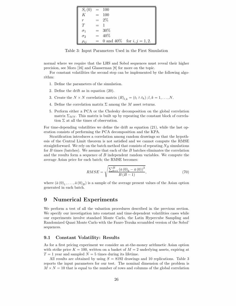
Si (0) = 100K = 100r = 2%T = 1σ1 = 30%σ2 = 40%ρij = 0 and 40% for i, j = 1, 2.

Table 3: Input Parameters Used in the First Simulation

normal where we require that the LHS and Sobol sequences must reveal their higherprecision, see Moro [16] and Glasserman [8] for more on the topic.

For constant volatilities the second step can be implemented by the following algo-rithm:

1. Define the parameters of the simulation.

2. Define the drift as in equation (20).

3. Create the N × N correlation matrix (R)l,k = (tl ∧ tk) ; l, k = 1, . . . , N .

4. Define the correlation matrix Σ among the M asset returns.

5. Perform either a PCA or the Cholesky decomposition on the global correlationmatrix ΣMN . This matrix is built up by repeating the constant block of correla-tion Σ at all the times of observation.

For time-depending volatilities we define the drift as equation (21), while the last op-eration consists of performing the PCA decomposition and the KPA.

Stratification introduces a correlation among random drawings so that the hypoth-esis of the Central Limit theorem is not satisfied and we cannot compute the RMSEstraightforward. We rely on the batch method that consists of repeating NB simulationsfor B times (batches). We assume that each of the B batches eliminates the correlationand the results form a sequence of B independent random variables. We compute theaverage Asian price for each batch; the RMSE becomes:

RMSE =

√∑Bb=1 (a (0)b − a (0))

2

B (B − 1), (70)

where (a (0)1 , . . . , a (0)B) is a sample of the average present values of the Asian optiongenerated in each batch.

9 Numerical Experiments

We perform a test of all the valuation procedures described in the previous section.We specify our investigation into constant and time-dependent volatilities cases whileour experiments involve standard Monte Carlo, the Latin Hypercube Sampling andRandomized Quasi Monte Carlo with the Faure-Tezuka scrambled version of the Sobol’sequences.

9.1 Constant Volatility: Results

As for a first pricing experiment we consider an at-the-money arithmetic Asian optionwith strike price K = 100, written on a basket of M = 2 underlying assets, expiring atT = 1 year and sampled N = 5 times during its lifetime.

All results are obtained by using S = 8192 drawings and 10 replications. Table 3reports the input parameters for our test. The nominal dimension of the problem isM ×N = 10 that is equal to the number of rows and columns of the global correlation

26

Standard MC LHS RQMC

PCA 7.195 (0.016) 7.157 (0.013) 7.1696 (0.0017)Cholesky 7.242 (0.047) 7.179 (0.022) 7.1689 (0.0071)

Table 4: Uncorrelation Case. Estimated Prices and Standard Errors.

Standard MC LHS RQMC

PCA 8.291 (0.053) 8.2868 (0.0073) 8.2831 (0.0016)Cholesky 8.374 (0.055) 8.293 (0.026) 8.2807 (0.0064)

Table 5: Correlation Case. Estimated Prices and Standard Errors.

matrix ΣMN . Paths are simulated by using both PCA and the Cholesky decompositionas in Dahl and Benth [6] and [7].

Table 4 and Table 5 show the results for the positive correlation and uncorrelatedcases, respectively. Simulated prices of the Asian basket options are in statistical ac-cordance, while the estimated RMSEs depend on the sampling strategy adopted. Therate of convergence of the RQMC estimation is higher than the other two methods.In particular it is ten times higher than the standard Monte Carlo method that wouldreturn the same accuracy with 100 × S drawings.

We observe that the PCA generation provides a better estimation both for LHSand RQMC, because these ones are more sensitive to the effective dimension, whilePCA causes no distinction for the standard MC. The effect is more pronounced forthe correlation case where the more complex structure of the global correlation matrixΣMN influences the estimation procedure.

As from a financial perspective, it is normal to find a higher price in the positivecorrelation case than in the uncorrelated one.

Moreover, we develop our analysis by investigating a very high-dimensional pricingproblem. A basket of M = 10 underlying assets is considered with N = 250 samplingtime points, the nominal dimension is d = 2500.

We run our simulation with the same parameters used by Imai and Tan [11] anduse the LSS for the high-dimensional QMC estimation as presented in the cited refer-ence. The authors concatenated 100 or 50 sets of 25 or 50 dimensional Sobol’ sequence,respectively. They exploit the LSS method in order to obtain a complete 2500 dimen-sional sample of digital net. Owen [19] is more restrictive; the author suggests to usescrambled digital sequences for the first five or ten components and LHS for the othersor to concatenate the principal components. We compare the results and investigatethe effective dimensions and the contribution of the eigenvalues of the global correlationmatrix. Table 6 reports input parameters for our test.

We compute the eigenvalues and eigenvectors of ΣMN . Property (10) of the Kro-necker product is fundamental in this computation and considerably reduces the com-putational burden and time. It results that the effective dimension is 143 or 170 forthe correlation and uncorrelation cases, respectively, are much smaller than the nom-inal one. Considering the first 143(170) columns, that is the first 143(170) principal

Si (0) = 100K = 100r = 4%T = 1

σi = 10% + i−1

940% for i = 1, . . . , 10

ρij = 0 and 40% for i, j = 1, . . . , 10

Table 6: Input Parameters Used in the Second Simulation

27

Uncorrelation Standard MC LHS RQMC

PCA 3.414(0.015) 3.4546(0.0054) 3.4438(0.0015)Cholesky 3.426(0.015) 3.4323(0.0070) 3.4518(0.0058)

Correlation Standard MC LHS RQMC

PCA 5.648(0.029) 5.6655(0.0032) 5.65750(0.00040)Cholesky 5.604(0.029) 5.670(0.013) 5.63710(0.019)

Table 7: Prices and RMSEs both for the correlated and uncorrelated case when 100% ofthe variance is considered.

Positive Correlation Zero Correlation

Price RMSE E Price RMSE E

5.262 0.090 5 2.596 0.041 55.294 0.088 10 3.190 0.047 105.433 0.088 15 3.212 0.047 155.528 0.091 20 3.239 0.047 205.484 0.092 25 3.289 0.047 255.445 0.090 30 3.375 0.048 305.653 0.015 147 3.452 0.010 170

Table 8: Prices and RMSE for different principal components when LHS is used.

components, the generating matrix C takes into account 99% of the total variance.Table 7 shows all the results we obtained. We concatenate 50 sets of 50-dimensional

randomized low-discrepancy sequences.We consider both the matrix of 2500 rows and 143(170) columns, excluding the

effects of the remaining principal components, and the complete ANOVA in order toinvestigate the effectiveness of our assumptions and hypotheses.

Table 8 presents the different Monte Carlo estimations with respect to the numberof eigenvalues when LHS is used.

Table 9 illustrates the values found by Imai and Tan [11]. Their results were obtainedassigning the importance of each component (not anymore PCA) with their LT method.All the estimations found are unbiased and in agreement with those presented in thecited references.

The Quasi-Monte Carlo method with LSS extension proves to be a powerful vari-ance reduction technique, particularly when coupled with the ANOVA-PCA decom-position. Moreover, the Kronecker product turns out to be a fast tool to generatemulti-dimensional Brownian paths. Indeed, the elapsed time to realize the same pathwithout using the properties of the Kronecker product is a lot higher.

The estimation with Cholesky decomposition gives higher uncertainty than the PCAapproach, meaning that a small amount of variance is lost. This is due to the fact thata relevant part of the variance is carried out by a few eigenvalues of the covariancematrix R. If these eigenvalues are observed, it can be noticed that only few of them arerelevant in the PCA analysis and they are much bigger than the ones of the matrix Σ.

Uncorrelation RQMC Correlation RQMC

PCA 3.4475(0.0023) PCA 5.65860(0.00072)Cholesky 3.426(0.0087) Cholesky 5.603(0.022)LT 3.4461(0.0012) LT 5.6780(0.00047)

Table 9: Estimated Results by Imai and Tan [13]

28

9.2 Constant Volatility: Comments

Based on these results, we can make the following conclusions:

1. The RQMC method and the use of the Faure-Tezuka scrambling technique pro-vide the best estimation among all the implemented procedures for both the“Correlation” and “Zero Correlation” cases. The correspondent RMSEs are thesmallest ones with a higher order of convergence with the same number of simu-lations.

2. The Kronecker product is a fast and efficient tool for generating multi-dimensionalBrownian paths with a low computational effort.

3. As compared to to the standard Monte Carlo and LHS approaches, the use ofscrambled low-discrepancy sequences provides more accurate results, at least forM × N ≤ 20, particularly with the PCA and LT-based methods.

4. The accuracy of the estimates is strongly dependent on the choice of the Choleskyor the PCA approach. In particular, independent of the simulation procedure(MC, LHS or RQMC), when using PCA decomposition the estimates are affectedby a smaller sampling error (smaller standard error).

9.3 Time-dependent Volatility: Results

The constant volatility hypothesis is the starting point for the pricing problem. A fur-ther improvement can be achieved by considering a time-dependent volatility function.

It is market practice to choose step-wise time-dependent volatilities. We want to in-vestigate a more complex dependence to test our new approach based on the Kroneckerproduct approximation. For this aim, we adopt an exponentially decaying functionhaving the following expression:

σi = σi(0) exp(− t

τi

)+ σi(+∞) (71)

where σi(0) + σi(+∞) = σi(0) is the initial volatility for the i-th asset, σi(+∞) is itsasymptotic volatility and τi its decay constant.

The particular time-dependent function leads to the following solution:

∫ tj∧tl

0

σi(t)σk(t)ρikdt = σi(0)σk(0)τik

(1 − exp

(− t

τik

))+

+σi(0)σk(+∞)τi

(1 − exp

(− t

τi

))+

+σk(0)σi(+∞)τik

(1 − exp

(− t

τik

))+

+σi(+∞)σk(+∞)t

where τik = τiτk/(τi + τk).The simulation implemented to obtain the price of an Asian option supposing time-

dependent volatility evolves as the constant volatility case. The main difference is theprocedure to reduce the dimension of the problem.

The parameters chosen for the simulation are listed in table 10.The initial volatilities are equal to those used in the constant volatility case. The

asymptotic volatility and the decay constant are the same among all the assets. Theseparameters are chosen in order to allow a comparison with respect to the constantvolatility case. Indeed, the price of the options is sensitive to the change of volatilityand in particular its decreasing trend should provide a lower price.

The basket consists of 10 underlying assets, the time grid has 250 equally spacedpoints and the number of runs is S = 8192 and 10 replications. Table 11 shows theresults coming from the simulation using the RQMC method both with the KPA andthe PCA for dimension reduction.

29

Si(0) = 100r = 4%T = 1yearσi(0) = 10% + i−1

940%

σi(+∞) = 9% for all iτi = 1.5yearK = 100ρij = 0 and 40% for i, j = 1, . . . , 10

Table 10: Input Parameters for the Time-depending Case

Positive Correlation (KPA) Zero Correlation(KPA)

Price 5.19658 Price 3.20784RMSE 0.00063 RMSE 0.00040

E 145 E 173

Positive Correlation (PCA) Zero Correlation(PCA)

Price 5.19856 Price 3.20147RMSE 0.00062 RMSE 0.00040

E 123 E 150

Table 11: Estimated Results for the Time-depending Case, ANOVA = 0.99

The KPA path-generation is efficient and fast. To have an idea of its speed, theelapsed times to obtain the generating matrix without exploiting the properties ofthe Kronecker product and no approximations are more than ten times higher. Asexpected, the simulation gives smaller prices with respect to the constant volatilitysituation, because a decreasing volatility function has been assigned.

The nominal dimensions of the problem E using PCA come out to be 126 and 150for the correlation and uncorrelation cases. When adopting the KPA the approximatednominal dimensions are higher, 145 and 173, respectively. If we would consider ANOVA= 0.9885 for the correlation case and ANOVA = 0.98805 for the uncorrelation casewe would get the PCA-found nominal dimension for ANOVA=0.99. We can judgethis small difference as negligible and consequently our approximating technique tobe efficient and leading to consistent results. As with N and M small, the Choleskydecomposition alone would require a small number of operations without giving anyorder of the importance for the random sources.

Tables 12 and 13 present the estimated prices when taking into account the fullcomponents. All the results are in accordance with those ones found with ANOVA=0.99.

Table 14 illustrates the sensitivity with respect to the number of principal com-ponents E: As in the constant volatility case it can be seen that the estimation isconvergent.

Moreover, we launch a new simulation with the LHS technique with the same setof parameters. We list the estimated results in table 15. The estimated prices havehigher RMSEs, confirming the fact that the RQMC approach provides a good variancereduction.

KPA PCA Cholesky

Price 3.20545 3.20390 3.1838RMSE 0.00040 0.00041 0.0091

Table 12: Uncorrelation Case. Estimated Prices and Standard Errors. ANOVA= 1.

30

KPA PCA Cholesky

Price 5.20060 5.20210 5.1946RMSE 0.00050 0.00058 0.0093

Table 13: Correlation Case. Estimated Prices and Standard Errors. ANOVA= 1.

Positive Correlation Zero Correlation

Price RMSE E Price RMSE E

5.7805 0.0079 5 2.6368 0.0038 54.9904 0.0081 10 2.9681 0.0042 105.0226 0.0081 15 3.1172 0.0043 155.1103 0.0081 20 3.0979 0.0043 205.1826 0.0083 25 3.1051 0.0043 255.1937 0.0082 30 3.1514 0.0043 30

Table 14: Prices and RMSEs for different principal components. Case: RQMC

Positive Correlation Zero Correlation

Price RMSE E Price RMSE E

4.874 0.016 5 3.121 0.089 55.093 0.016 10 3.118 0.085 105.097 0.016 15 3.122 0.086 155.131 0.016 20 3.072 0.086 205.145 0.016 25 3.163 0.088 255.201 0.016 30 3.110 0.089 30

Table 15: Prices and RMSEs for different principal components. Case: LHS

31

9.4 Time-Dependent Volatility: Comments

According to the results we have found in the time-dependent case, it is possible todraw the following conclusions:

1. RQMC with LSS is a general approach that does not depend on the chosen pricedynamic.

2. The KPA we propose, provides unbiased estimations with a reduction of thecomputational cost. In the framework we investigate, KPA returns a highernominal dimension, as expected, but only relatively to a negligible amount ofvariance.

3. KPA is a lot faster than the straightforward PCA because it exploits the prop-erties of the Kronecker product and the boomerang shaped matrices. The ad hocCholesky decomposition algorithm we develop is fundamental for the KPA. Wedo not report computational times because we expect that further improvementscan be done.

4. KPA and PCA can be considered both valid as path-generation methods to sup-port the ANOVA and the identifications of effective dimensions.

32

References

[1] P. Acworth, M. Broadie, and P. Glasserman. 1998. A comparison of some MonteCarlo and quasi-Monte Carlo methods for option pricing. In Monte Carlo andQuasi-Monte Carlo Methods 1996: Proceedings of a conference at the Universityof Salzburg, Austria, July 9-12, 1996, ed. H. Niederreiter, P. Hellekalek, G. Larcherand P. Zinterhof. Lecture Notes in Statistics 127. Springer-Verlag, New York.

[2] P. Boyle, M. Broadie and P. Glasserman. 1995. Recent Advances in Simulationfor Security Pricing. Proceedings of the 1995 Winter Simulation Conference. C.Alexopoulos, K. Kang, W.R. Lilegdon and D. Goldsman,ed.s.

[3] P. Boyle, M. Broadie and P. Glasserman. 1997. Monte Carlo Methods for SecurityPricing. Journal of Economics Dynamics and Control. 21: 1267-1321

[4] R. Caflisch, W. Morokoff, and A. Owen. 1997. Valuation of mortgage-backed se-curities using Brownian bridges to reduce effective dimension. Journal of Compu-tational Finance 1 (1):2746.

[5] N. Cufaro-Petroni. 1996. Lezioni di Calcolo delle Probabilita. Edizioni dal Sud.Modugno. 1996.

[6] L.O. Dahl, F.E. Benth. 2001. Valuation of the Asian Basket Option with Quasi-Monte Carlo Techniques and Singular Value Decomposition. Pure Mathematics.5.

[7] L.O. Dahl, F.E. Benth. 2002. Fast Evaluation of the Asian Option by SingularValue Decomposition. Proceedings of the Conference: Monte Carlo and Quasi-Monte Carlo Methods 2000. K.-T. Fang, F.J.Hickernell, H. Niederreiter,ed.s. 201-214, Springer-Verlag Berlin Heidelberg 2002.

[8] P. Glasserman. 2004. Monte Carlo Methods in Financial Engineering. Springer-Verlag New York. 2004.

[9] G.H. Golub, C.F. Van Loan. 1996. Matrix Computations 3rd Ed. The Johns Hop-kins University Press 1996.

[10] H.S. Hong, F.J. Hickernell. 2000. Implementing Scrambled Digital Nets. Unpub-lished Technical Report, Hong Kong Baptist University.

[11] J. Imai, K.S. Tan. 2002. Enhanced Quasi-Monte Carlo Method with DimensionReduction. Proceedings of the 2002 Winter Simulation Conference. D.J. Medeiros,E. Ycesan,C.-H. Chen, J.L. Snowdon and J.M. Charnes,ed.s.

[12] J. Imai, K.S. Tan. 2005. Minimizing Effective Dimension using Linear Transforma-tion. Monte Carlo and Quasi-Monte Carlo Methods 2004. H. Niederreiter editor,Springer-Verlag 2005.

[13] J. Imai, K.S. Tan. 2007. A General Dimension Reduction Technique for Deriva-tive Pricing. Journal of Computational Finance. Volume 10/Number 2. Winter2006/2007. Pages 129-155.

[14] A.N. Langville, W.J. Stewart. 2004. The Kronecker Products and Stochastic Au-tomata Networks. Journal of Computational and Applied Mathematics Volume167, Issue 2, 1 June 2004, Pages 429-447

[15] J.R. Koehler, A. Owen. 1996. Computer Experiment. Handbook of Statistics. De-sign and Analysis of Experiments. S. Ghosh and C.R. Rao,ed.s.

[16] B. Moro. 1995. The Full Monte. Risk(8)(Feb):57-58.

[17] H. Niederreiter. 1992. Random Number Generation and Quasi-Monte Carlo Meth-ods. S.I.A.M., Philadelphia 1992.

[18] A. Owen. 2003. Quasi-Monte Carlo Sampling. Chapter for a SIGGRAPH 2003course. San Diego.

33

[19] A. Owen. 1998. Monte Carlo Estension of Quasi-Monte Carlo. Proceedings of the1998 Winter Simulation Conference. D.J. Medeiros, E.F. Watson, J.S. Carsonand M.S. Manivannan,ed.s.

[20] A. Owen. 1998. Latin Supercube Sampling for Very High-dimensional Simulations.ACM Transaction on Modelling and Computer Simulation. 8: 71-102.

[21] A. Owen. 2002. Variance and Discrepancy with Alternative Scramblings. ACMTransactions on Computational Logic, Vol V.

[22] N. Pitsianis, C.F. Van Loan. 1993. Approximation with Kronecker Products. Lin-ear Algebra for Large Scale and Real Time application. M.S. Moonen and G.H.Golub, ed.s. Kluwer Academic Publishers, 293-314.

[23] W.H. Press, S.A. Teukolsky, W.T. Vetterling, B.P. Flannery. 1992. NumericalRecipes in C: the Art of Technical Computing. Cambridge University Press.

[24] R. Rebonato. 2004. Volatility and Correlation or the Perfect Hedger and the Fox.John Wiley & Sons 2004.

[25] C.F. Van Loan. 2000. The Ubiquitous Kronecker Product. Journal of Computa-tional and Applied Mathematics. 123: 85-100.

[26] J. Vecer. 2001. A new PDE approach for pricing arithmetic average Asian options.Journal of Computational Finance, Vol. 4, No. 4, 105-113.

[27] J. Vecer. 2002. Unified Asian Pricing. Risk, Vol. 15, No. 6, 113-116.

34