. . . . . . . . Monte Carlo Methods for Nonlinear PDEs Arash Fahim, University of Michigan Joint work with Nizar Touzi, Xavier Warin Joint work with Erhan Bayraktar Arash Fahim (U of Michigan) Monte Carlo Methods for Nonlinear PDEs 1 / 65
Transcript
. . . . . .
.
...... Monte Carlo Methods for Nonlinear PDEs
Arash Fahim, University of MichiganJoint work with Nizar Touzi, Xavier Warin
Joint work with Erhan Bayraktar
Arash Fahim (U of Michigan) Monte Carlo Methods for Nonlinear PDEs 1 / 65
. . . . . .
Sketch of the presentation
...1 Motivations
...2 Linear and Nonlinear Monte Carlo Methods
...3 Fully nonlinear Monte Carlo
Arash Fahim (U of Michigan) Monte Carlo Methods for Nonlinear PDEs 2 / 65
. . . . . .
Motivations
Terminology I
.
......
(Ω, Ft,P): Filtered probability space, Q: the martingale measure, E orE: the expectation, Wtt≥0, d-dimensional Brownian motion
Risky assets (S(i)t )d
i=1
Money market account with interest rate = rt .
θ: trading strategy
X θt : Wealth process at time t based on the self–financing strategy θ
Et,s = E[·|St = s]
Arash Fahim (U of Michigan) Monte Carlo Methods for Nonlinear PDEs 3 / 65
. . . . . .
Motivations
Pricing American option I
.Markov derivatives..
......Pay–off: ϕ(ST )Price at time t : V (t , s) = supτ Et,s[e−
∫ τt rsdsϕ(Sτ )].
.PDE..
......0 = min−Vt − rsDV − s2σ2D2V + rV , v − ϕ and V (T , ·) = ϕ(·).∆-Hedging: θt = DV (t ,St) for t < τ .
.Longstaff-Schwartz..
......
No analytical solution for the PDE in higher dimensions:
V (tk , s) := maxEt,s[e−
∫ tk+1tk
rsdsV (Stk+1)], ϕ(s).In the above, Et,s is approximated by projection on a set of polynomials, usingonly one set of sample paths.
Arash Fahim (U of Michigan) Monte Carlo Methods for Nonlinear PDEs 4 / 65
. . . . . .
Motivations
Pricing American option II
.Monte Carlo Hedging and Greeks..
......
Euler approximation of St : Sh = σsWh and ∆Wh := Wt+h − Wt :
∆t(s) ≈ 1σsh
Et,s[V (t , s + σsWh)(∆Wh)]
Γt(s) ≈ 1σ2s2h2 Et,s[V (t , s + σsWh)((∆Wh)
2 − h)].
Arash Fahim (U of Michigan) Monte Carlo Methods for Nonlinear PDEs 5 / 65
Arash Fahim (U of Michigan) Monte Carlo Methods for Nonlinear PDEs 6 / 65
. . . . . .
Motivations
Indifference pricing I
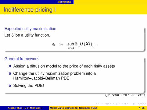
.Expected utility maximization..
......
Let U be a utility function.
v0 := supθ∈A
E[U(X θ
T)].
.General framework..
......
Assign a diffusion model to the price of each risky assets
Change the utility maximization problem into aHamilton–Jacobi–Bellman PDE
Solving the PDE!
Arash Fahim (U of Michigan) Monte Carlo Methods for Nonlinear PDEs 7 / 65
. . . . . .
Motivations
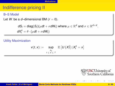
Indifference pricing II.B–S Model..
......
Let W· be a d–dimensional BM (r = 0).
dSt = diag(St)(µdt + σdWt) where µ ∈ Rd and σ ∈ Rd×d .
dX θt = θ · (µdt + σdWt)
.Utility Maximization..
......
v(t , x) := supθs
t ≤ s ≤ T
E[U(X θ
T)|X θ
t = x]
Arash Fahim (U of Michigan) Monte Carlo Methods for Nonlinear PDEs 8 / 65
. . . . . .
Motivations
Indifference pricing III
.HJB equation..
......
v(T , x) = U(x)
0 =− vt − supθ∈R
(12θ2σ2vxx + θµvx
)=− vt +
12µt(σσt)−1µ
(vx)2
vxx.
This PDE is fully non–linear.For exponential utility the solution can be find analytically.The dimension of the equation does not increase with the number of assets.
Arash Fahim (U of Michigan) Monte Carlo Methods for Nonlinear PDEs 9 / 65
. . . . . .
Motivations
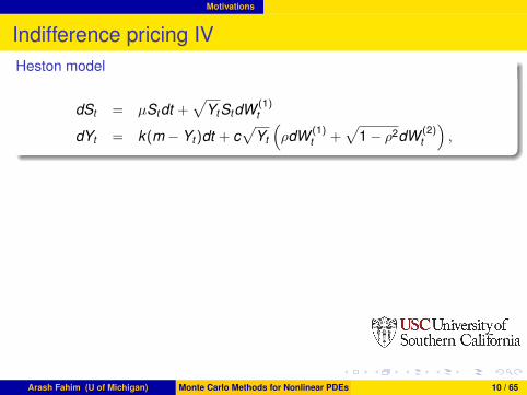
Indifference pricing IV.Heston model..
......
dSt = µStdt +√
YtStdW (1)t
dYt = k(m − Yt)dt + c√
Yt
(ρdW (1)
t +√
1 − ρ2dW (2)t
),
Arash Fahim (U of Michigan) Monte Carlo Methods for Nonlinear PDEs 10 / 65
. . . . . .
Motivations
Indifference pricing V
.HJB equation..
......
v(T , x , y) = U(x)
0 =− vt − k(m − y)vy − 12
c2yvyy − supθ∈R
(12θ2yvxx + θ(µvx + ρcyvxy )
)=− vt − k(m − y)vy − 1
2c2yvyy +
(µvx + ρcyvxy )2
2yvxx.
The dimension of fully non–linear PDE do increases with the number ofstochastic volatility models.
Arash Fahim (U of Michigan) Monte Carlo Methods for Nonlinear PDEs 11 / 65
. . . . . .
Motivations
Indifference pricing VI
.Vasicek, Heston and CEV-SV models..
......
drt = κ(b − rt)dt + ζdW (0)t
dS(i)t = µiS
(i)t dt + σi
√Y (i)
t S(i)tβi
dW (i,1)t , β2 = 1,
dY (i)t = ki
(mi − Y (i)
t
)dt + ci
√Y (i)
t dW (i,2)t .
Arash Fahim (U of Michigan) Monte Carlo Methods for Nonlinear PDEs 12 / 65
. . . . . .
Motivations
Indifference pricing VII.HJB equation..
......
U(x) = v(T , r , x , s1, y1, y2)
0 = −vt − (Lr + LY + LS1)v − rxvx
+((µ1 − r)vx + σ2
1y1s2β1−11 vxs1)
2
2σ21y1s2β1−2
1 vxx+
((µ2 − r)vx)2
2σ22y2vxx
Lr v = κ(b − r)vr +12ζ2vrr , LY v =
2∑i=1
ki (mi − yi) vyi +12
c2i yivyi yi ,
and LS1v = µ1s1vs1 −
12σ2
1s1y1vs1s1 .
Arash Fahim (U of Michigan) Monte Carlo Methods for Nonlinear PDEs 13 / 65
. . . . . .
Fully non-linear parabolic PDEs
Monte Carlo methods for PDE
.The curse of dimensionality..
......
PDEs appear in many areas including finance, image processing,...The analytic solutions usually refuse to exist and we need to approximate thesolution.The deterministic approximation methods like FD, FEM, ... are highlysensitive w.r.t. dimension of the space so that they result non efficientalgorithms in dimensions d > 3.However, the Monte Carlo scheme is less sensitive to dimension and couldbe used to develop numerical schemes.
Arash Fahim (U of Michigan) Monte Carlo Methods for Nonlinear PDEs 14 / 65
. . . . . .
Fully non-linear parabolic PDEs
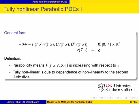
Fully nonlinear Parabolic PDEs I
.General form..
......
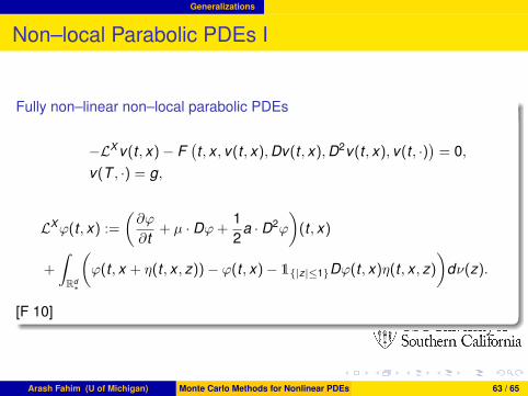
−∂tv − F (t , x , v(t , x),Dv(t , x),D2v(t , x)) = 0, [0,T )× Rd
v(T , ·) = g.
Definition:
- Parabolicity means F (t , x , r , p, γ) is increasing with respect to γ.
- Fully non–linear is due to dependence of non–linearity to the secondderivative.
Arash Fahim (U of Michigan) Monte Carlo Methods for Nonlinear PDEs 15 / 65
. . . . . .
Fully non-linear parabolic PDEs
Fully nonlinear Parabolic PDEs II.Separation into linear and fully nonlinear parts..
......
−LX v − F (t , x , v(t , x),Dv(t , x),D2v(t , x)) = 0, [0,T )× Rd
v(T , ·) = g.
where LXφ := ∂φ∂t + µ · Dφ+ 1
2σTσ · D2φ is the infinitesimal generator of
dXt = µdt + σdWt
and LX + F = ∂∂t + F and F is still parabolic.
.Choice of µ and σ..
......
ut +12u = ut +
14u+ 1
4u = ut +18u+ 3
8u but notut +
34u+ −1
4 u
Arash Fahim (U of Michigan) Monte Carlo Methods for Nonlinear PDEs 16 / 65
. . . . . .
Fully non-linear parabolic PDEs
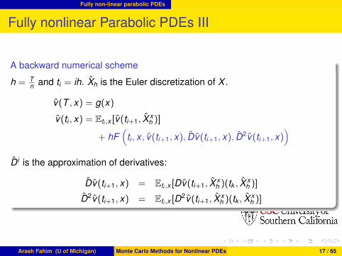
Fully nonlinear Parabolic PDEs III
.A backward numerical scheme..
......
h = Tn and ti = ih. Xh is the Euler discretization of X .
v(T , x) = g(x)
v(ti , x) = Eti ,x [v(ti+1, X xh )]
+ hF(
ti , x , v(ti+1, x), Dv(ti+1, x), D2v(ti+1, x))
Di is the approximation of derivatives:
Dv(ti+1, x) = Eti ,x [Dv(ti+1, X xh )(tk , X
xh )]
D2v(ti+1, x) = Eti ,x [D2v(ti+1, X x
h )(tk , Xxh )]
Arash Fahim (U of Michigan) Monte Carlo Methods for Nonlinear PDEs 17 / 65
. . . . . .
Fully non-linear parabolic PDEs
Fully nonlinear Parabolic PDEs IV
.Key Lemma: Integration by part..
......
For every exponentially bounded smooth function φ : Rd → R, we have:
E[Diφ(x + σWh)] = E[φ(x + σWh)Hhi (Wh)],
where Hh = (Hh0 ,H
h1 ,H
h2 ) and
Hh0 (x) = 1,Hh
1 (x) =1hσ′(x)−1Wh,
Hh2 (x) =
1h2σ
′(x)−1(WhW ′h − hId×d )σ(x)−1
One dimensional case
Arash Fahim (U of Michigan) Monte Carlo Methods for Nonlinear PDEs 18 / 65
. . . . . .
Fully non-linear parabolic PDEs
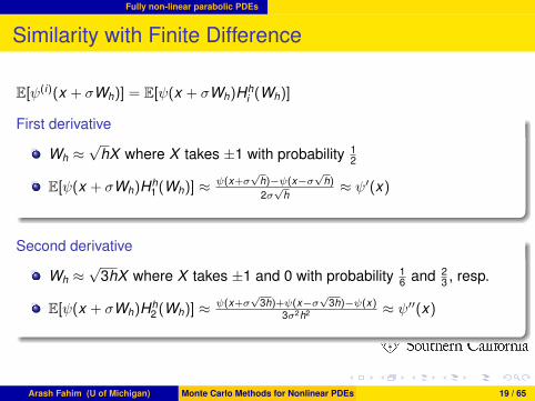
Similarity with Finite Difference
E[ψ(i)(x + σWh)] = E[ψ(x + σWh)Hhi (Wh)]
.First derivative..
......
Wh ≈√
hX where X takes ±1 with probability 12
E[ψ(x + σWh)Hh1 (Wh)] ≈ ψ(x+σ
√h)−ψ(x−σ
√h)
2σ√
h≈ ψ′(x)
.Second derivative..
......
Wh ≈√
3hX where X takes ±1 and 0 with probability 16 and 2
3 , resp.
E[ψ(x + σWh)Hh2 (Wh)] ≈ ψ(x+σ
√3h)+ψ(x−σ
√3h)−ψ(x)
3σ2h2 ≈ ψ′′(x)
Arash Fahim (U of Michigan) Monte Carlo Methods for Nonlinear PDEs 19 / 65
. . . . . .
Fully non-linear parabolic PDEs
Similarity with Finite Difference
E[ψ(i)(x + σWh)] = E[ψ(x + σWh)Hhi (Wh)]
.First derivative..
......
Wh ≈√
hX where X takes ±1 with probability 12
E[ψ(x + σWh)Hh1 (Wh)] ≈ ψ(x+σ
√h)−ψ(x−σ
√h)
2σ√
h≈ ψ′(x)
.Second derivative..
......
Wh ≈√
3hX where X takes ±1 and 0 with probability 16 and 2
3 , resp.
E[ψ(x + σWh)Hh2 (Wh)] ≈ ψ(x+σ
√3h)+ψ(x−σ
√3h)−ψ(x)
3σ2h2 ≈ ψ′′(x)
Arash Fahim (U of Michigan) Monte Carlo Methods for Nonlinear PDEs 19 / 65
. . . . . .
Probabilistic interpretation for Parabolic PDEs
Why Feynman-Kac doesn’t work for nonlinear PDEs I
.Linear PDEs..
......
0 = −vt − LX v + kv and v(T , ·) = g(·).
LX = 12σ
Tσ · D2v −+mu · Dv .
v(t , x) = E
[exp
(−∫ T
tk(Xs)ds
)g(XT )
∣∣∣Xt = x
].
where dXt = µdt + σ · dWt .
Arash Fahim (U of Michigan) Monte Carlo Methods for Nonlinear PDEs 20 / 65
. . . . . .
Probabilistic interpretation for Parabolic PDEs
Why Feynman-Kac doesn’t work for nonlinear PDEs II
.Totter–Kato..
......
Φ(1)h [g](t , x) = Et,x [g(Xt+h)] the semi–group generated by 0 = −vt − LX v and
Φ(2)h [g](t , x) = exp(−
∫ t+ht ksds)g(x) the semi–group generated by
0 = −vt + kv . Then, (h → 0)
v(t , x) ≈ Φ(1)h Φ(2)
h · · · Φ(1)h Φ(2)
h [g](t , x)
Hopefully, two semi–groups commute:
v(t , x) ≈ Φ(1)T−t Φ
(2)T−t [g](t , x)
→ Et,x
[exp
(−∫ T
tk(Xs)ds
)g(XT )
].
But, when the equation is non–linear, they don’t commute.
Arash Fahim (U of Michigan) Monte Carlo Methods for Nonlinear PDEs 21 / 65
. . . . . .
Probabilistic interpretation for Parabolic PDEs
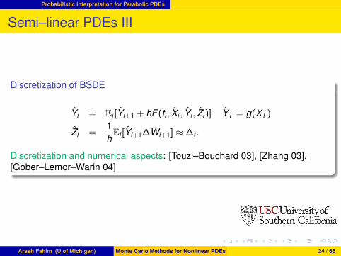
Semi–linear PDEs I.Semi–linear equations..
......
0 = −vt −12σTσ · D2v − µ · Dv − F (v ,Dv)
v(T , ·) = g(·).
Possibly no classic solution. The solution should be considered in viscositysense.Example: Interest rate spread.
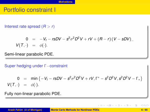
Arash Fahim (U of Michigan) Monte Carlo Methods for Nonlinear PDEs 22 / 65
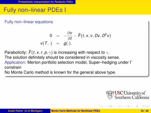
Parabolicity: F (t , x , r , p, γ) is increasing with respect to γ.The solution definitely should be considered in viscosity sense.Application: Merton portfolio selection model, Super–hedging under ΓconstrainNo Monte Carlo method is known for the general above type.
Arash Fahim (U of Michigan) Monte Carlo Methods for Nonlinear PDEs 25 / 65
. . . . . .
Probabilistic interpretation for Parabolic PDEs
Fully non–linear PDEs II
.2BSDE..
......
dYt = F (Yt ,Zt , Γt)dt − ZtdXt
dZt = Atdt + ΓtdXt
YT = g(XT ).
If v is the classical solution of semi–linear PDE,Yt = v(t ,Xt), Zt = Dv(t ,Xt),Γt = D2v(t ,Xt), At = LX Dv(t ,Xt).Theory is recently developed its first steps by [Cheridito–Soner–Touzi–Victoir07] and [Soner–Touzi–Zhang 10]×4.
Arash Fahim (U of Michigan) Monte Carlo Methods for Nonlinear PDEs 26 / 65
. . . . . .
Probabilistic interpretation for Parabolic PDEs
Fully non–linear PDEs III
.Discretization of 2BSDE..
......
Yi = Ei [Yi+1 + hF (ti , Xi , Yi , Zi , Γi)] YT = g(XT )
Zi =1hEi [Yi+1∆Wi+1] ZT = Dg(XT )
Γi =1hEi [Zi+1∆Wi+1]
Alternative scheme.
Arash Fahim (U of Michigan) Monte Carlo Methods for Nonlinear PDEs 27 / 65
. . . . . .
Asymptotics
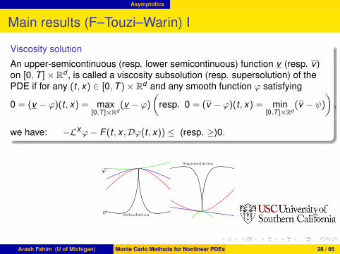
Main results (F–Touzi–Warin) I.Viscosity solution..
......
An upper-semicontinuous (resp. lower semicontinuous) function v (resp. v )on [0,T ]× Rd , is called a viscosity subsolution (resp. supersolution) of thePDE if for any (t , x) ∈ [0,T )× Rd and any smooth function φ satisfying
0 = (v − φ)(t , x) = max[0,T ]×Rd
(v − φ)
(resp. 0 = (v − φ)(t , x) = min
[0,T ]×Rd(v − ψ)
),
we have: −LXφ− F (t , x ,Dφ(t , x)) ≤ (resp. ≥)0.
Subsolution
Supersolution
φ
v
Arash Fahim (U of Michigan) Monte Carlo Methods for Nonlinear PDEs 28 / 65
. . . . . .
Asymptotics
Main results (F–Touzi–Warin) II.Comparison principle..
......
We say that fully non-linear equation has comparison for bounded functions iffor any bounded upper semicontinuous subsolution v and any bounded lowersemicontinuous supersolution v on [0,T )× Rd , satisfying v(T , ·) ≤ v(T , ·),we have v ≤ v .
.Assumption F..
......
...1 F is Lipschitz-continuous with respect to (x , r , p, γ) uniformly in t .
...2 |F (·, ·, 0, 0, 0)|∞ <∞.
...3 F is elliptic (increasing w.r.t. γ).
...4 ∇γF .a−1 ≤ 1 where a := σ′σ on Rd × R× Rd × Sd .
...5 Fp ∈ Image(Fγ) and∣∣F T
p F−γ Fp
∣∣∞ < +∞.
Arash Fahim (U of Michigan) Monte Carlo Methods for Nonlinear PDEs 29 / 65
. . . . . .
Asymptotics
Main results (F–Touzi–Warin) III
.Convergence Thm: F–Touzi–Warin..
......
Assume F and comparison for the PDE. For every bounded Lipschitz functiong, there exists a bounded function v so that
vh −→ v locally uniformly.
In addition, v is the unique bounded viscosity solution of fully non-linearproblem.
.Proof of Convergence..
......The proof of convergence relies on the method of Barles and Souganidis forviscosity solutions (Not directly applicable).
Arash Fahim (U of Michigan) Monte Carlo Methods for Nonlinear PDEs 30 / 65
. . . . . .
Asymptotics
Main results (F–Touzi–Warin) IV
.Monotonicity..
......
Should be: If φ ≤ ψ then Th[φ] ≤ Th[ψ].But it is: If φ ≤ ψ then Th[φ] ≤ Th[ψ] + ChE[(ψ − φ)(t + h, X x
h )].
.Stability........The family vh is uniformly bounded.
.Consistency..
......
When h → 0, c → 0 and (t ′, x ′) → (t , x):
1h(ψ + c − Th[ψ + c])(t ′, x ′) → −vt − LX v − F (t , x ,Dv(t , x)).
Arash Fahim (U of Michigan) Monte Carlo Methods for Nonlinear PDEs 31 / 65
. . . . . .
Asymptotics
Main results (F–Touzi–Warin) V
.Final condition..
......
When h → 0 and (t ′, x ′) → (T , x): vh(t ′, x ′) → g(x). (This result is neithernecessary for nor provided by Barles–Souganidis but very crucial in thiscontext, because of the form of the equation.)
.Regularity of approximate solution..
......
vh is Lipschitz in x and 12 -Holder on t . What we need for above result is the
later. In F-Touzi-Warin, we used x Lipschitz continuity to show t 12 -Holder
continuity. Later on, this step was skipped in the future work on PDEs ongeneral domains.
Arash Fahim (U of Michigan) Monte Carlo Methods for Nonlinear PDEs 32 / 65
. . . . . .
Asymptotics
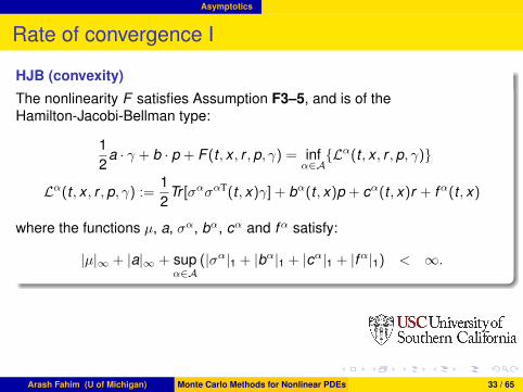
Rate of convergence I.HJB (convexity)..
......
The nonlinearity F satisfies Assumption F3–5, and is of theHamilton-Jacobi-Bellman type:
The proof of rate of convergence is obtained through Krylov, Barles andJakobsen method of shaking coefficients and switching system approximationof Barles and Jakobsen (Not directly applicable).
Arash Fahim (U of Michigan) Monte Carlo Methods for Nonlinear PDEs 34 / 65
. . . . . .
Asymptotics
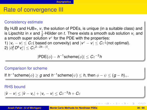
Rate of convergence III.Consistency estimate..
......
By HJB and HJB+, v , the solution of PDEs, is unique (in a suitable class) andis Lipschitz in x and 1
2 -Holder on t . There exists a smooth sub solution vε anda smooth super solution vε for the PDE with the properties:1) |vε − v | ≤ Cε( based on convexity) and |vε − v | ≤ Cε
13 (not optimal).
2) |∂kt Dk vεε | ≤ Cε2−2k−|l|.
|PDE(ϕ)− h−1scheme(ϕ)| ≤ Cε−3h
.Comparison for scheme........If h−1scheme(ϕ) ≥ g and h−1scheme(ψ) ≤ h, then ϕ− ψ ≤ (g − h)+.
.RHS bound........|v − v | ≤ |v − vε|+ |vε − v | ≤ Cε−3h + Cε
Arash Fahim (U of Michigan) Monte Carlo Methods for Nonlinear PDEs 35 / 65
. . . . . .
Implementation
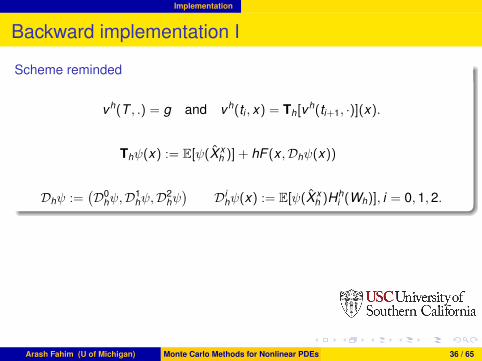
Backward implementation I.Scheme reminded..
......
vh(T , .) = g and vh(ti , x) = Th[vh(ti+1, ·)](x).
Thψ(x) := E[ψ(X xh )] + hF (x ,Dhψ(x))
Dhψ :=(D0
hψ,D1hψ,D2
hψ)
Dihψ(x) := E[ψ(X x
h )Hhi (Wh)], i = 0,1, 2.
Arash Fahim (U of Michigan) Monte Carlo Methods for Nonlinear PDEs 36 / 65
. . . . . .
Implementation
Backward implementation II.Implementation..
......
...1 ti = iTn .
...2 Generating N sample paths from the Euler discretization of Xt ; Xt .
(X (j)ti ,∆W (j)
ti+1)|0 = t0, · · · , tn = T , j = 1, · · · ,N.
...3 Start from terminal condition g(·). And proceed backward in time.
...4 Knowing vh(ti+1, X(j)ti+1
)s for j = 1, · · · ,N , then one calculates
vh(ti , X(k)ti )s for k = 1, · · · ,N using the scheme.
Arash Fahim (U of Michigan) Monte Carlo Methods for Nonlinear PDEs 37 / 65
. . . . . .
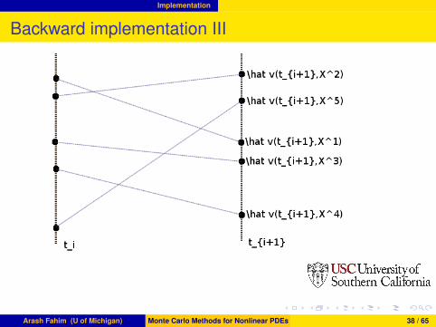
Implementation
Backward implementation III
Arash Fahim (U of Michigan) Monte Carlo Methods for Nonlinear PDEs 38 / 65
. . . . . .
Implementation
Backward implementation IV
.4th step..
......
To compute vh(ti , x), one needs to approximate:
E[vh(ti+1, Xti+1)|Xti = x ]
E[vh(ti+1, Xti+1)∆Wti+1 |Xti = x ]
E[vh(ti+1, Xti+1)((∆Wti+1)2 − h)|Xti = x ]
Arash Fahim (U of Michigan) Monte Carlo Methods for Nonlinear PDEs 39 / 65
. . . . . .
Implementation
Approximation of conditional expectations I.Kernel methods..
......
Y = v(t + h, Xt+h)H ih and X = Xt . Informally;
E[Y |X = x ] =E[Y δx(X )]
E[δx(X )]≈ E[Yεκ(x − X )]
E[εκ(x − X )]
where εκ → δ0. In terms of a sample (X i ,Y i)Ni=1.∑
i εκ(Xi − x)Y i∑
i εκ(X i − x)
Arash Fahim (U of Michigan) Monte Carlo Methods for Nonlinear PDEs 40 / 65
. . . . . .
Implementation
Approximation of conditional expectations II
.Projection methods..
......
Y = v(t + h, Xt+h)H ih and X = Xt . Formally;
E[Y |X = x ] ≈∑
k
ckψk (x)
Coefficients ck s should be determined so that the L2 approximation error beminimum.
Arash Fahim (U of Michigan) Monte Carlo Methods for Nonlinear PDEs 41 / 65
. . . . . .
Implementation
Approximation of conditional expectations III
.Malliavin methods..
......
Y = v(t + h, Xt+h)H ih and X = Xt . Formally;
E[Y |X = x ] =E[Y δx(X )]
E[δx (X )]
E[Y δx(X )] = E[Y 1X>xδt0] where δt
0 is Skorokhod integral which dependsonly on the path of X from 0 to t .
Arash Fahim (U of Michigan) Monte Carlo Methods for Nonlinear PDEs 42 / 65
. . . . . .
Implementation
Approximation of conditional expectations IV.Stochastic scheme..
......
TNh [ψ](t , x) := EN
[ψ(t + h, X x
h )]+ hF
(·, Dhψ
)(t , x),
TNh [ψ](t , x) := −Kh[ψ] ∨ TN
h [ψ](t , x) ∧ Kh[ψ]
where
Dhψ(t , x) := EN[ψ(t + h, X t,x
h )Hh(t , x)], Kh[ψ] := ∥ψ∥∞(1 + C1h) + C2h,
and
C1 =14|F T
p F−γ Fp|∞ + |Fr |∞ and C2 = |F (t , x , 0,0, 0)|∞.
Arash Fahim (U of Michigan) Monte Carlo Methods for Nonlinear PDEs 43 / 65
. . . . . .
Implementation
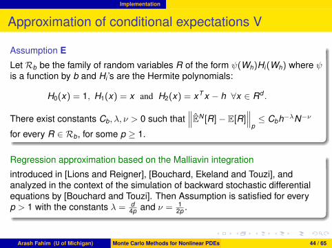
Approximation of conditional expectations V
.Assumption E..
......
Let Rb be the family of random variables R of the form ψ(Wh)Hi(Wh) where ψis a function by b and Hi ’s are the Hermite polynomials:
H0(x) = 1, H1(x) = x and H2(x) = xT x − h ∀x ∈ Rd .
There exist constants Cb, λ, ν > 0 such that∥∥∥EN [R]− E[R]
∥∥∥p≤ Cbh−λN−ν
for every R ∈ Rb, for some p ≥ 1.
.Regression approximation based on the Malliavin integration..
......
introduced in [Lions and Reigner], [Bouchard, Ekeland and Touzi], andanalyzed in the context of the simulation of backward stochastic differentialequations by [Bouchard and Touzi]. Then Assumption is satisfied for everyp > 1 with the constants λ = d
4p and ν = 12p .
Arash Fahim (U of Michigan) Monte Carlo Methods for Nonlinear PDEs 44 / 65
. . . . . .
Implementation
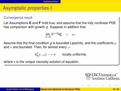
Asymptatic properties I.Convergence result..
......
Let Assumptions E and F hold true, and assume that the fully nonlinear PDEhas comparison with growth q. Suppose in addition that
limh→0
hλ+2Nνh = ∞.
Assume that the final condition g is bounded Lipschitz, and the coefficients µand σ are bounded. Then, for almost every ω:
vhNh(·, ω) −→ v locally uniformly,
where v is the unique viscosity solution of equation.
Arash Fahim (U of Michigan) Monte Carlo Methods for Nonlinear PDEs 45 / 65
. . . . . .
Implementation
Asymptatic properties II
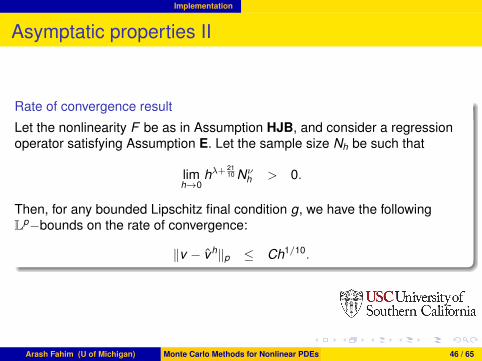
.Rate of convergence result..
......
Let the nonlinearity F be as in Assumption HJB, and consider a regressionoperator satisfying Assumption E. Let the sample size Nh be such that
limh→0
hλ+2110 Nν
h > 0.
Then, for any bounded Lipschitz final condition g, we have the followingLp−bounds on the rate of convergence:
∥v − vh∥p ≤ Ch1/10.
Arash Fahim (U of Michigan) Monte Carlo Methods for Nonlinear PDEs 46 / 65
. . . . . .
Numerical experiments
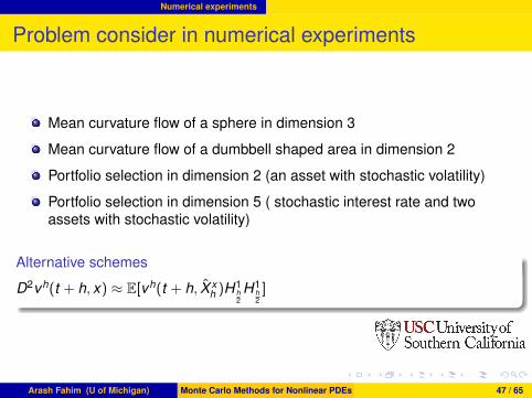
Problem consider in numerical experiments
Mean curvature flow of a sphere in dimension 3
Mean curvature flow of a dumbbell shaped area in dimension 2
Portfolio selection in dimension 2 (an asset with stochastic volatility)
Portfolio selection in dimension 5 ( stochastic interest rate and twoassets with stochastic volatility)
.Alternative schemes..
......D2vh(t + h, x) ≈ E[vh(t + h, X x
h )H1h2H1
h2]
Arash Fahim (U of Michigan) Monte Carlo Methods for Nonlinear PDEs 47 / 65
. . . . . .
Numerical experiments
3-d sphere
Arash Fahim (U of Michigan) Monte Carlo Methods for Nonlinear PDEs 48 / 65
. . . . . .
Numerical experiments
2-d dumbbell
Arash Fahim (U of Michigan) Monte Carlo Methods for Nonlinear PDEs 49 / 65
. . . . . .
Numerical experiments
Portfolio selection in dimension 2 I.Heston model..
......
dSt = µStdt +√
YtStdW (1)t
dYt = k(m − Yt)dt + c√
Yt
(ρdW (1)
t +√
1 − ρ2dW (2)t
),
.Utility maximization..
......v0 := sup
θ∈AE[−exp
(−ηX θ
T)].
Arash Fahim (U of Michigan) Monte Carlo Methods for Nonlinear PDEs 50 / 65
. . . . . .
Numerical experiments
Portfolio selection in dimension 2 II
.HJB equation..
......
v(T , x , y) = −e−ηx
0 =− vt − k(m − y)vy − 12
c2yvyy
− supθ∈R
(12θ2yvxx + θ(µvx + ρcyvxy )
)=− vt − k(m − y)vy − 1
2c2yvyy +
(µvx + ρcyvxy )2
2yvxx.
.Zariphopoulou semi-explicit solution..
......v(t , x , y) = −e−ηx
∥∥∥exp(− 1
2
∫ Ttµ2
Ysds)∥∥∥
L1−ρ2
Arash Fahim (U of Michigan) Monte Carlo Methods for Nonlinear PDEs 51 / 65
. . . . . .
Numerical experiments
Portfolio selection in dimension 2 III.Separation into linear and fully non–linear part..
......
−vt−k(m−y)vy−12
c2yvyy−12σ2vxx+F
(y ,Dv ,D2v
)= 0, v(T , x , y) = −e−ηx ,
F (y , z, γ) =12σ2γ11 +
(µz1 + ρcyγ12)2
2yγ11.
Arash Fahim (U of Michigan) Monte Carlo Methods for Nonlinear PDEs 52 / 65
. . . . . .
Numerical experiments
Portfolio selection in dimension 2 IV
.Truncation of the non–linearity..
......Fε,M(y , z, γ) :=
12σ2γ11 − sup
ε≤θ≤M
(12θ2(y ∨ ε)γ11 + θ(µz1 + ρc(y ∨ ε)γ12
),
.Choice of diffusion..
......
dX (1)t = σdW (1)
t , and dX (2)t = k(m − X (2)
t )dt + c√
X (2)t dW (2)
t .
µ = 0.15, c = 0.2, k = 0.1, m = 0.3, Y0 = m, ρ = 0, x0 = 1, T = 1 thenv0 = −0.3534.
Arash Fahim (U of Michigan) Monte Carlo Methods for Nonlinear PDEs 53 / 65
. . . . . .
Numerical experiments
2 dimensional 1
Arash Fahim (U of Michigan) Monte Carlo Methods for Nonlinear PDEs 54 / 65
. . . . . .
Numerical experiments
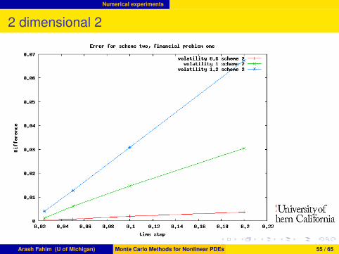
2 dimensional 2
Arash Fahim (U of Michigan) Monte Carlo Methods for Nonlinear PDEs 55 / 65
. . . . . .
Numerical experiments
Portfolio selection in dimension 5 I.Vasicek, Heston and CEV-SV models..
......
drt = κ(b − rt)dt + ζdW (0)t
dS(i)t = µiS
(i)t dt + σi
√Y (i)
t S(i)tβi
dW (i,1)t , β2 = 1,
dY (i)t = ki
(mi − Y (i)
t
)dt + ci
√Y (i)
t dW (i,2)t .
Arash Fahim (U of Michigan) Monte Carlo Methods for Nonlinear PDEs 56 / 65
. . . . . .
Numerical experiments
Portfolio selection in dimension 5 II
.HJB equation..
......
0 = −vt − (Lr + LY + LS1)v − rxvx
+((µ1 − r)vx + σ2
1y1s2β1−11 vxs1)
2
2σ21y1s2β1−2
1 vxx+
((µ2 − r)vx)2
2σ22y2vxx
Lr v = κ(b − r)vr +12ζ2vrr , LY v =
2∑i=1
ki (mi − yi) vyi +12
c2i yivyi yi ,
and LS1v = µ1s1vs1 −
12σ2
1s1y1vs1s1 .
Arash Fahim (U of Michigan) Monte Carlo Methods for Nonlinear PDEs 57 / 65
. . . . . .
Numerical experiments
Portfolio selection in dimension 5 III.Separation into linear and fully non–linear part..
......
−vt − (Lr + LY + LS1)v − 1
2σ2vxx + F
((x , r , s1, y1, y2),Dv ,D2v
)= 0,
v(T , x , r , s1, y1, y2) = −e−ηx ,
F (u, z, γ) =12σ2γ11 − x1x2z1 +
((µ1 − x2)z1 + σ21x4x2β1−1
3 γ1,3)2
2σ21x4x2β1−2
3 γ11
+((µ2 − x2)z1)
2
2σ22x5γ11
,
where u = (x1, · · · , x5).
Arash Fahim (U of Michigan) Monte Carlo Methods for Nonlinear PDEs 58 / 65
. . . . . .
Numerical experiments
Portfolio selection in dimension 5 IV.Truncation of the non–linearity..
......
Fε,M(u, z, γ) :=12σ2γ11 − x1x2z1 + sup
ε≤|θ|≤M
(θ · (µ− r1)z1
+θ1σ21(x4 ∨ ε)(x3 ∨ ε)2β1−1γ13
+12(θ2
1σ21(x3 ∨ ε)(x4 ∨ ε)2β1−2 + θ2
2σ22(x5 ∨ ε))γ11
,
Arash Fahim (U of Michigan) Monte Carlo Methods for Nonlinear PDEs 59 / 65
. . . . . .
Numerical experiments
Portfolio selection in dimension 5 V
.Choice of diffusion..
......
dX (1)t = σdW (0)
t ,
dX (2)t = κ(b − X (2)
t )dt + ζdW (1)t ,
dX (3)t = µ1X (3)
t dt + σ1
√X (4)
t X (3)t
β1dW (1,1)
t ,
dX (4)t = k1(m1 − X (4)
t )dt + c1
√X (4)
t dW (1,2)t ,
dX (5)t = k2(m2 − X (5)
t )dt + c2
√X (5)
t dW (2,2)t .
Arash Fahim (U of Michigan) Monte Carlo Methods for Nonlinear PDEs 60 / 65
. . . . . .
Numerical experiments
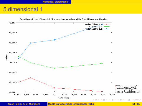
5 dimensional 1
Arash Fahim (U of Michigan) Monte Carlo Methods for Nonlinear PDEs 61 / 65
. . . . . .
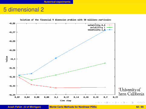
Numerical experiments
5 dimensional 2
Arash Fahim (U of Michigan) Monte Carlo Methods for Nonlinear PDEs 62 / 65