Monte Carlo sampling of Wigner functions and surface ... · Monte Carlo sampling of Wigner...

Takustraße 7D-14195 Berlin-Dahlem

GermanyKonrad-Zuse-Zentrumfur Informationstechnik Berlin

SUSANNA KUBE, CAROLINE LASSER, MARCUS WEBER

Monte Carlo sampling of Wignerfunctions and surface hopping quantum

dynamics

ZIB-Report 07-17 (Dezember 2007)

Monte Carlo sampling of Wigner functions and

surface hopping quantum dynamics

Susanna Kube∗ Caroline Lasser† Marcus Weber‡

Abstract

Wigner functions are functions on classical phase space, which are inone-to-one correspondence to square integrable functions on configura-tion space. For molecular quantum systems, classical transport of Wignerfunctions provides the basis of asymptotic approximation methods in thehigh energy regime. The article addresses the sampling of Wigner func-tions by Monte Carlo techniques. The approximation step is realized byan adaption of the Metropolis algorithm for real-valued functions withdisconnected support. The quadrature, which computes values of theWigner function, uses importance sampling with a Gaussian weight func-tion. The numerical experiments combine the sampling with a surfacehopping algorithm for non-adiabatic quantum dynamics. In agreementwith theoretical considerations, the obtained results show an accuracy oftwo to four percent.

AMS MSC 2000: 62D05, 65D30, 81S30, 81Q20

Keywords: Metropolis Monte Carlo, approximation, quadrature, oscil-lating functions, quantum dynamics, non-adiabatic, surface hopping

∗Zuse Institute Berlin, Takustraße 7, D-14195 Berlin, Germany ([email protected])†FU Berlin, Arnimallee 6, D-14195 Berlin, Germany ([email protected])‡Zuse Institute Berlin, Takustraße 7, D-14195 Berlin, Germany ([email protected])

1

2 S. Kube, C. Lasser, M. Weber

Contents

Introduction 3

1 Wigner functions 81.1 Basic properties . . . . . . . . . . . . . . . . . . . . . . . . . . . . 81.2 Husimi functions . . . . . . . . . . . . . . . . . . . . . . . . . . . 91.3 Ambiguity functions . . . . . . . . . . . . . . . . . . . . . . . . . 11

2 Numerical set up 112.1 Initial data . . . . . . . . . . . . . . . . . . . . . . . . . . . . . . 122.2 Grid based surface hopping . . . . . . . . . . . . . . . . . . . . . 12

2.2.1 Single Gaussian wave packet . . . . . . . . . . . . . . . . 132.2.2 Superposition of Gaussian wave packets . . . . . . . . . . 132.2.3 Excited harmonic oscillator state . . . . . . . . . . . . . . 13

3 Monte Carlo sampling 143.1 Metropolis Monte Carlo . . . . . . . . . . . . . . . . . . . . . . . 14

3.1.1 Standard approach . . . . . . . . . . . . . . . . . . . . . . 143.1.2 Sampling from a real-valued function . . . . . . . . . . . . 153.1.3 Disconnected support . . . . . . . . . . . . . . . . . . . . 15

3.2 Importance Sampling . . . . . . . . . . . . . . . . . . . . . . . . . 163.2.1 Standard approach . . . . . . . . . . . . . . . . . . . . . . 163.2.2 Embedded importance sampling . . . . . . . . . . . . . . 17

4 Gaussian wave packet 184.1 Approximation . . . . . . . . . . . . . . . . . . . . . . . . . . . . 18

4.1.1 Simple Monte Carlo . . . . . . . . . . . . . . . . . . . . . 184.1.2 Metropolis Monte Carlo . . . . . . . . . . . . . . . . . . . 19

4.2 Integration . . . . . . . . . . . . . . . . . . . . . . . . . . . . . . 204.2.1 Standard importance sampling . . . . . . . . . . . . . . . 214.2.2 Embedded importance sampling . . . . . . . . . . . . . . 22

5 Superposition of Gaussian wave packets 225.1 Approximation . . . . . . . . . . . . . . . . . . . . . . . . . . . . 225.2 Integration . . . . . . . . . . . . . . . . . . . . . . . . . . . . . . 255.3 Approximation of the Husimi function . . . . . . . . . . . . . . . 26

6 Excited harmonic oscillator state 27

Conclusion 29

A Reference solutions 30

B Analytical Wigner transformation 31

C Position densities by density estimation 33

Monte Carlo sampling and surface hopping 3

Introduction

The fundamental equation of non-relativistic quantum molecular dynamics isthe time-dependent Schrodinger equation

i~∂τψ(τ, q) = − ~2

2m∆qψ(τ, q) + V (q)ψ(τ, q), ψ(0, q) = ψ0(q).

It is a linear partial differential equation with a unique global solution providedby the spectral theorem. Indeed, under reasonable regularity and growth as-sumptions on the potential V : Rd → R, the Hamiltonian P = − ~2

2m∆q + V (q)is a self-adjoint operator in L2(Rd), and the solution can be written as

ψ(τ, q) = e−iPτ/~ψ0(q).

For most molecules, the dimension d of the configuration spaces Rd is large. Intypical applications, one might want to consider up to thirty degrees of freedom.On top of that, the solution ψ(t, q) exhibits oscillations both in time and inspace. For quantifying the oscillatory behavior, one switches to atomic units bysetting ~ = 1 and introduces the crucial semiclassical parameter

ε =√

1/m.

On the long time scale t = τ/ε, on which the distinguished dynamical featuresdevelop, the Schrodinger equation writes as

iε∂tψ(t, q) = − ε2

2 ∆qψ(t, q) + V (q)ψ(t, q), ψ(0, q) = ψ0(q).

Then, all oscillations are roughly characterized by the frequency 1/ε, whichtypically ranges between hundred and thousand.

The conventional interpretation of quantum mechanics does not assign anyphysical meaning to the wave function ψ(t, q) itself, but to quadratic quantitiesof it. The probability for finding the quantum system at time t within the setΩ ⊂ Rd is ∫

Ω

|ψ(t, q)|2 dq.

Consequently, the initial data are always normalized, and the unitary time-evolution guarantees

∀t ∈ R : ‖ψ(t)‖L2 = 1.

The expectation value for the position and the momentum of the system attime t are for example

〈ψ(t), qψ(t)〉L2 , 〈ψ(t),−iε∇qψ(t)〉L2 .

More generally, one associates with smooth functions a : R2d → C on classicalphase space a Weyl quantized operator op(a) acting in L2(Rd) by the appropri-ate interpretation of the definition

op(a)ψ(q) = (2πε)−d

∫R2d

a( 12 (q + x), p)eip·(q−x)/εψ(x) dxdp.

The corresponding expectation values

〈ψ(t), op(a)ψ(t)〉L2


then specialize to components of the position and momentum expectation bychoosing a(q, p) = qj and a(q, p) = pj , respectively.

In the semiclassical regime with small parameter 0 < ε 1, the directapproach to quadratic quantities is advantageous, since their dynamics are lessoscillatory than those of the wave function itself. The celebrated Egorov theoremprovides the following approximation (Theorem IV.10 in [24]). Let

q = p, p = −∇qV (q)

be the classical Hamiltonian system associated to the Schrodinger operator P ,and let Φt : R2d → R2d denote its flow. Then,

〈ψ(t), op(a)ψ(t)〉L2 =⟨ψ0, op(a Φ−t)ψ0

⟩L2 +O(ε2),

where the constant of the error term depends on time t and bounds on derivativesof the function a and the potential V , which are greater or equal than orderthree. In particular, the Egorov theorem provides an exact description for thedynamics of harmonic oscillator, whose potential is a quadratic function. Onthe level of this general asymptotic approximation, oscillations in time do notshow up any more and space oscillations must only be resolved for the initialwave function ψ0.

Moreover, all expectation values associated with a wave function ψ can beexpressed by its Wigner function W (ψ) : R2d → R, which is a function onclassical phase space. The definition

W (ψ)(q, p) = (2π)−d

∫Rd

eix·p ψ(q − ε2x)ψ(q + ε

2x) dx (1)

grants

〈ψ, op(a)ψ〉L2 =∫

R2d

W (ψ)(q, p)a(q, p) dq dp

for all square integrable functions ψ and smooth symbols a, where all integralshave to be interpreted carefully, of course. The Wigner function has first beenproposed by Wigner, further developed by Moyal, and reintroduced in the con-text of signal analysis by Ville [31, 19, 29]. Its main properties will be brieflydiscussed in §1. From the Wigner point of view, the Egorov theorem rephrasesas

W (ψ(t)) = W (ψ0) Φt +O(ε2), (2)

where the relation has to be understood in a weak sense. One then deduces asimple particle method, which is built of the following steps.

Initial sampling. One samples the Wigner function W (ψ0) of the initial wavefunction ψ0 to obtain a family of phase space points (q1, p1), . . . , (qN , pN ).

Classical transport. The phase space points are transported along the curvesof the Hamiltonian system q = p, p = −∇qV (q) until the desired time t.

Final evaluation. One regards the values of the initial Wigner functionW (ψ0)in (q1, p1), . . . (qN , pN ) as an approximation of the values of the Wignerfunction W (ψ(t)) in the points Φt(q1, p1), . . . ,Φt(qN , pN ) and computesexpectation values.


It is our aim here to contribute to the initial sampling step. Hence, wepursue the following two main objectives. First, the generation of phase spacepoints according to the Wigner function W (ψ) of a typical square integrablefunction ψ. Second, the computation of the Fourier integral in equation (1),which defines the value of the Wigner function W (ψ) in a given phase spacepoint (q, p). The first task is related to the problem of approximation, while thesecond one concerns numerical quadrature.

The wave functions ψ we have in mind are laser-excited eigenstates of semi-classical Schrodinger operators

− ε2

2 ∆q + V (q),

as they arise in the context of Born-Oppenheimer approximation. The con-figuration vector q contains the molecule’s nuclear coordinates, the semiclas-sical parameter ε is of the same size as the inverse of the square root of theaverage nuclear mass, and the potential V gives the nth eigenvalue of theelectronic Schrodinger equation for a given nuclear configuration q. Hence,we consider wave functions with the following properties: exponential decay,high order differentiability, microlocalization around a few phase space pointsc0, . . . , cs ∈ R2d.

The current chemical literature mostly considers Gaussian wave packets cen-tered in a single phase space point z0 = (q0, p0), which are of the form

gz0(q) = (πε)−d/4 exp(− 1

2ε |q − q0|2 + iεp0 · (q − q0)

).

Their Wigner function is a Gaussian

W (gz0)(q, p) = (πε)−d exp(− 1

ε |q − q0|2 − 1ε |p− p0|2

),

whose approximation is unproblematic, of course. However, if the Wigner func-tion were not computable analytically, one would have to solve a GaussianFourier integral of the type

f(p− p0) =∫

Rd

eix·(p−p0)e−ε4 |x|

2dx

numerically, whose relative condition number

κf (p− p0) =|p− p0|

|f(p− p0)||∇f(p− p0)| = 2

ε |p− p0|2

reflects the oscillatory behavior of the integrand for large distances |p − p0|.Also the approximation problem suffers from oscillations as soon as the Wignerfunction localizes around several phase space points. An illustrative exampleis the superposition of two Gaussian wave packets with centers in z1, z2 ∈ R2d,whose Wigner function

W (gz1 + gz2)(q, p) = W (gz1)(q, p) +W (gz2)(q, p) + 2c(q, p)

contains the dangerous cross term [9]

c(q, p) = (πε)−de−|(q,p)−z+|2/ε cos(

1ε (p+ · q− − ((q, p)− z+) ∧ z−)

),


which localizes around the arithmetic mean z+ = (z1 +z2)/2 and oscillates witha frequency proportional to z− = z1 − z2.

To summarize, one faces a highly oscillatory problem of approximation andnumerical quadrature in a high dimensional setting. Our aim is the systematicexploration of how a Monte Carlo approach can deal with the situation. Forthe approximation, we propose an adaption of the Metropolis algorithm, whichjumps between predefined phase space regions and accounts for the negativevalues of the Wigner function. The quadrature uses importance sampling witha Gaussian proposal distribution and is complemented by a convergence test forthe oscillatory regime.

For the numerical validation we consider a variant of the above mentionedparticle method, which belongs to the family of surface hopping algorithms.These algorithms are widely used for the simulation of non-adiabatic quantumdynamics as they are generated by Schrodinger systems with conical intersec-tions. The Schrodinger system

iε∂tψ(t, q) = − ε2

2 ∆qψ(t, q) + V (q)ψ(t, q), ψ(0, q) = ψ0(q)

with real symmetric potential matrix

V (q) = 12 trV (q) +

(v1(q) v2(q)v2(q) −v1(q)

)has a conical intersection, if the eigenvalues λ+(q) and λ−(q) of V (q) coincideon a smooth submanifold of codimension two of the configuration space. In thiscase, there is a suitable set of coordinates such that near the crossing set

q ∈ Rd | λ+(q) = λ−(q)

the two eigenvalue surfaces Rd → R, q 7→ λ±(q) look like two cones touching eachother in their end points. Conical intersections are ubiquitous for the descrip-tion of radiationless decay and isomerization processes of polyatomic molecules[2]. The eigenvalues λ±(q) are also eigenvalues of an electronic Schrodingeroperator, which parametrically depends on the nuclear position q. Their in-tersection violates the adiabatic Born-Oppenheimer approximation in the fol-lowing sense. If χ±(q) denotes a normalized eigenvector of the matrix V (q)and ψ±(t, q) = 〈χ±(q), ψ(t, q)〉C2 the solution’s component in the correspondingeigenspace, then it may happen that

ψ−(0) = 0 & ∃t : ψ+(t) = O(1), ε→ 0.

That is, the wave function performs a leading order non-adiabatic transitionfrom one eigenspace to the other, from the plus space to the minus space orvice versa. For systems with conical intersections the particle method has to besupplemented by a surface hopping step.

Initial sampling. One samples the Wigner functions W (ψ±(0)) to obtain twofamilies of phase space points (q±1 , p

±1 ), . . . , (q±N± , p

±N±) with associated

real-valued weights w±1 , . . . , w±N± , which are the values of the Wigner func-

tion W (ψ±(0)) in these points.

Classical transport. The phase space points are transported along the curvesof the corresponding Hamiltonian system q = p, p = −∇qλ

±(q).


Surface hopping. Whenever a trajectory t 7→ (qt, pt) passes one of its minimalsurface gaps at a point (q, p), that is whenever the function

t 7→ (λ+(qt)− λ−(qt))

attains a local minimum, then a branching occurs. The transition branchcarries the old weight times the Landau-Zener factor

T (q, p) = exp(−πε

|v(q)|2

|dv(q)p|

),

where dv(q) denotes the 2 × d gradient matrix of v(q) = (v1(q), v2(q)),and starts a new trajectory in (q, p), which is associated with the othereigenvalue. The remaining branch continues the old trajectory and carriesthe old weight times 1− T (q, p).

Final evaluation. At the desired time t, one obtains two families of phasespace points (q±1 , p

±1 ), . . . , (q±M± , p

±M±) and weights w±1 , . . . , w

±M± , which

approximate the values of the Wigner function W (ψ±(t)) in these points.One computes the final expectation values.

The chemical physics’ literature contains an overwhelming variety of surfacehopping algorithms, which all differ in the way the non-adiabatic transitionsare performed. The method considered here is called single switch surface hop-ping, since its constitutive branching condition allows for non-adiabatic switchesjust at minimal surface gaps along trajectories, whereas most of the establishedalgorithms have random jumps at every time step of the discretization [6]. More-over, the single switch approach is the only way of surface hopping, which hasbeen derived from a rigorous mathematical analysis of Schrodinger systems withgeneric crossings [16, 14]. The main observables for the evaluation of the initialsampling are the energy level populations P±(t) = ‖ψ±(t)‖2

L2 , which give theprobability of the wave function to be in the plus or minus eigenspace at time t.In terms of Wigner functions they express as the phase space integral

P±(t) =∫

R2d

W (ψ±(t))(q, p) dq dp.

If W±(t, q, p) denotes the value of the phase space functions at time t generatedby the single switch method, then the generalization of the Egorov theoremguarantees

W (ψ±(t))(q, p) = W±(t, q, p) +O(ε1/8),

where the relation holds in a weak sense (Theorem 2.2 in [14]) . However, all thenumerical experiments so far have even shown a convergence rate of order

√ε,

see [15, 14] and §5.3 later on.Our article is organized as follows. In section §1, basic properties of Wigner

functions are discussed. §2 contains the detailed set up for the numerical exper-iments, while §3 presents the Monte Carlo methods for the approximation andthe quadrature problem at hand. §4, §5, and §6 validate the proposed methodfor initial wave functions, which are a single Gaussian wave packet, a superpo-sition of two Gaussian wave packets, and an excited harmonic oscillator state,respectively. Then, we offer an assessment of the obtained results in the finalsection.


1 Wigner functions

Considering dimension d = 1, the phase space R2 of classical and quantummechanics can also be thought of as the time-frequency plane of signal analysis.In this context the Wigner function has been called the musical score [1]. Sinceexpositions of its main properties have been given many times, see for examplechapter 1.8 in [3] or chapter 4.3 in [7], we will only focus on those, which arerelevant for its intended Monte Carlo sampling to start an asymptotic particlemethod.

1.1 Basic properties

By the Fourier transform of a square integrable function ψ ∈ L2(Rd) we alwaysmean the ε-scaled Fourier transform

(Fψ)(p) = (2πε)−d/2

∫Rd

e−iq·p/ε ψ(q) dq.

Then, the Wigner function

W (ψ)(q, p) = (2πε)−d

∫Rd

eix·p/ε ψ(q − 12x)ψ(q + 1

2x) dx

is the inverse Fourier transform of the dilated product x 7→ ψ(q− 12x)ψ(q+ 1

2x).Hence,

W (ψ) : R2d → R

is a square integrable function on phase space, and one obtains for any q0 ∈ Rd

with ψ(q0) 6= 0 the inversion formula

ψ(q) = ψ(q0)−1

∫Rd

ei(q−q0)·p/εW (ψ)( 12 (q + q0), p) dp.

Let a : R2d → C be a smooth function on phase space and op(a) the associatedWeyl quantized pseudodifferential operator,

op(a)ψ(q) = (2πε)−d

∫R2d

a( 12 (q + x), p) eip·(q−x)/ε ψ(x) dxdp.

Then,

〈ψ, op(a)ψ〉L2 =∫

R2d

W (ψ)(q, p) a(q, p) dq dp.

In addition to the relation with expectation values, the marginals are the posi-tion and momentum density,∫

Rd

W (ψ)(q, p) dp = |ψ(q)|2,∫

Rd

W (ψ)(q, p) dq = |(Fψ)(p)|2,

and consequently ∫R2d

W (ψ)(q, p) dq dp = ‖ψ‖2L2 .

The balance between position and momentum is also observed in the identity

W (ψ)(q, p) = W (Fψ)(p,−q).


Moreover, W (ψ)(q, p) 6= 0 implies that (q, p) lies in the convex hull of

supp(ψ)× supp(Fψ).

The interpretation of the Wigner function as a phase space density has thedefect, that it might attain negatives values. Indeed,

W (ψ)(0, 0) = −(επ)−d‖ψ‖2L2

for odd functions ψ(q) = −ψ(−q). However, in an averaged sense the negativityis rather mild because of the sharp Garding inequality (Chapter 2.10 in [17]).For smooth non-negative functions a ≥ 0 there exists a positive constant C =C(a) > 0 depending on derivative bounds of a such that∫

R2d

W (ψ)(q, p) a(q, p) dq dp ≥ −Cε‖ψ‖2L2 .

1.2 Husimi functions

An alternative quadratic phase space representation of square integrable func-tions ψ ∈ L2(Rd) is the Husimi function [11], which can be defined as a suitablyscaled Gauß transform of the Wigner function,

H(ψ)(q, p) = (επ)−d

∫R2d

W (ψ)(x, ξ) e−(|q−x|2+|p−ξ|2)/ε dxdξ.

A few lines of computation yield the non-negativity of the Husimi function,which can be expressed as the modulus squared of the FBI transform

H(ψ)(q, p) = |T (ψ)(q, p)|2

with

T (ψ)(q, p) = 2−d/2(πε)−3d/4

∫Rd

ei(q−y)·p/ε e−|q−y|2/(2ε) ψ(y) dy.

The FBI transform is the inner product of the wave function with a Gaussianwave packet. The initials stand for Fourier, Bros and Iagolnitzer [12]. Aver-ages of the Husimi and the Wigner function are rather close in the followingasymptotic sense. For smooth phase space functions a one obtains∫

R2d

H(ψ)(q, p) a(q, p) dq dp

= (επ)−d

∫R4d

W (ψ)(x, ξ) e−(|q−x|2+|p−ξ|2)/ε a(q, p) dxdξ dq dp

=∫

R2d

W (ψ)(x, ξ) a(x, ξ) dxdξ +O(ε).

The above relation is due to the properties of the phase space Gaussian

G(q, p) = (επ)−d e−(|q|2+|p|2)/ε,

whose integral is one, while its mean is zero, and its variance is ε/2. A secondorder Taylor approximation of the function a then gives for the convolution

(a ∗G)(q, p) = a(q, p) +O(ε),


where the error depends on second order derivatives of a. The Husimi functionof the Gaussian wave packet gz0 is the Gaussian

H(gz0)(q, p) = (2πε)−d exp(− 1

2ε |q − q0|2 − 12ε |p− p0|2

),

whose variance is larger than that of the corresponding Wigner function. Hence,in general the Husimi function’s marginals are not position and momentumdensities. For a superposition of two Gaussian wave packets with centers inz1, z2 ∈ R2d one computes

H(gz1 + gz2)(q, p) = H(gz1)(q, p) +H(gz2)(q, p) + 2c(q, p),

where the cross term

c(q, p) = (2πε)−d e−18ε |z−|

2exp(− 1

2ε |(q, p)− z+|2)cos(

12ε (c1,2 − (q, p) ∧ z−)

)expectedly localizes around the mean z+ = (z1 + z2)/2. The cosine has aphase shift c1,2 = q(z1) · p(z1) − q(z2) · p(z2) and oscillates with a frequencyproportional to the difference z− = z1− z2. However, due to the damping term,which is exponentially small in |z−|2, the oscillations are absorbed by the tailsof the two Gaussian functions H(gz1) and H(gz2). For the Husimi function,the Egorov theorem holds with a remainder of order ε, which is worse than theerror of order ε2 valid for Wigner functions. Indeed, if ψ(t) solves the scalarSchrodinger equation

iε∂tψ = Pψ, ψ(0) = ψ0,

and if Φt denotes the associated classical flow, then

H(ψ(t)) = H(ψ0) Φt +O(ε) (3)

holds in a weak sense. The remainder term of order ε is sharp, since∫R2d

H(ψ(t))(q, p) a(q, p) dq dp =∫

R2d

W (ψ(t))(q, p) (a ∗G)(q, p) dq dp

=∫

R2d

W (ψ0)(q, p)((a ∗G) Φ−t

)(q, p) dq dp+O(ε2)

=∫

R2d

W (ψ0)(q, p)((a Φ−t) ∗G

)(q, p) dq dp+O(ε)

=∫

R2d

H(ψ0)(q, p) (a Φ−t)(q, p) dq dp+O(ε),

where the estimate of order ε2 stems from the classical transport of Wignerfunctions and the order ε term from the relation(

(a ∗G) Φ−t)(q, p) = a(Φ−t(q, p)) +O(ε) =

((a Φ−t) ∗G

)(q, p) +O(ε).

Hence, the error in the Egorov theorem (3) depends on derivatives bounds fora and Φt, which are of order greater or equal than two.


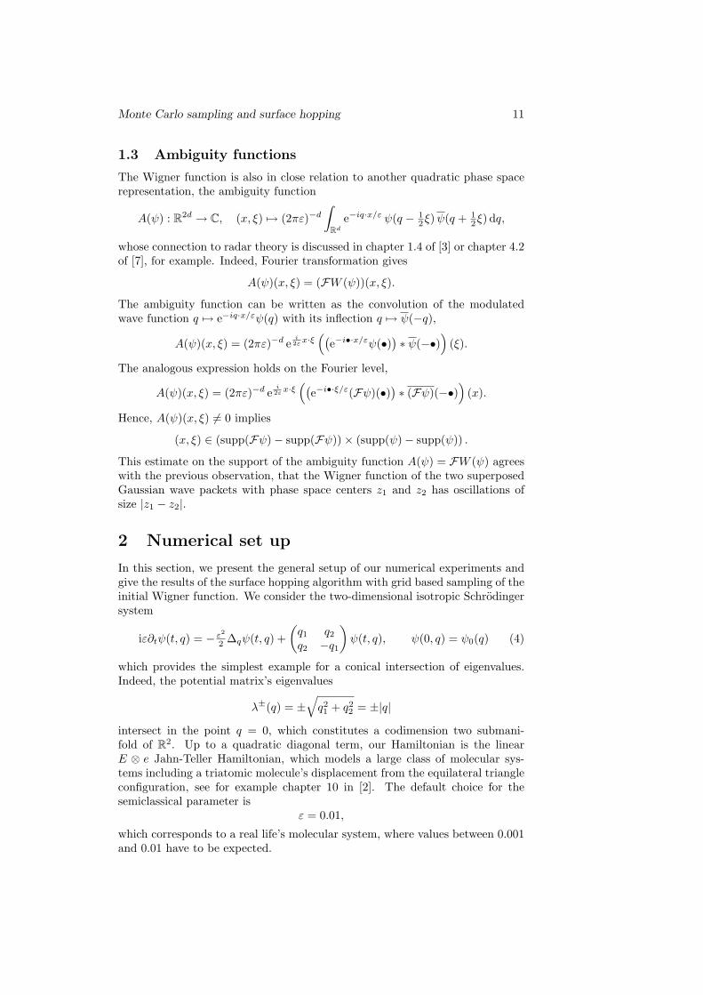
1.3 Ambiguity functions

The Wigner function is also in close relation to another quadratic phase spacerepresentation, the ambiguity function

A(ψ) : R2d → C, (x, ξ) 7→ (2πε)−d

∫Rd

e−iq·x/ε ψ(q − 12ξ)ψ(q + 1

2ξ) dq,

whose connection to radar theory is discussed in chapter 1.4 of [3] or chapter 4.2of [7], for example. Indeed, Fourier transformation gives

A(ψ)(x, ξ) = (FW (ψ))(x, ξ).

The ambiguity function can be written as the convolution of the modulatedwave function q 7→ e−iq·x/εψ(q) with its inflection q 7→ ψ(−q),

A(ψ)(x, ξ) = (2πε)−d ei2ε x·ξ

((e−i•·x/εψ(•)

)∗ ψ(−•)

)(ξ).

The analogous expression holds on the Fourier level,

A(ψ)(x, ξ) = (2πε)−d ei2ε x·ξ

((e−i•·ξ/ε(Fψ)(•)

)∗ (Fψ)(−•)

)(x).

Hence, A(ψ)(x, ξ) 6= 0 implies

(x, ξ) ∈ (supp(Fψ)− supp(Fψ))× (supp(ψ)− supp(ψ)) .

This estimate on the support of the ambiguity function A(ψ) = FW (ψ) agreeswith the previous observation, that the Wigner function of the two superposedGaussian wave packets with phase space centers z1 and z2 has oscillations ofsize |z1 − z2|.

2 Numerical set up

In this section, we present the general setup of our numerical experiments andgive the results of the surface hopping algorithm with grid based sampling of theinitial Wigner function. We consider the two-dimensional isotropic Schrodingersystem

iε∂tψ(t, q) = − ε2

2 ∆qψ(t, q) +(q1 q2q2 −q1

)ψ(t, q), ψ(0, q) = ψ0(q) (4)

which provides the simplest example for a conical intersection of eigenvalues.Indeed, the potential matrix’s eigenvalues

λ±(q) = ±√q21 + q22 = ±|q|

intersect in the point q = 0, which constitutes a codimension two submani-fold of R2. Up to a quadratic diagonal term, our Hamiltonian is the linearE ⊗ e Jahn-Teller Hamiltonian, which models a large class of molecular sys-tems including a triatomic molecule’s displacement from the equilateral triangleconfiguration, see for example chapter 10 in [2]. The default choice for thesemiclassical parameter is

ε = 0.01,

which corresponds to a real life’s molecular system, where values between 0.001and 0.01 have to be expected.


2.1 Initial data

The initial data are the pointwise product of a scalar wave function ψ+0 : R2 → C

with an eigenvector χ+(q) of the potential matrix associated with the eigenvalueλ+(q),

ψ0(q) = ψ+0 (q)χ+(q).

Such initial data are typically chosen for the simulation of quantum moleculardynamics after excitation of the molecule by light or a laser-pulse. We haveconsidered three different scalar functions ψ+

0 ,

ψ+0 ∈

gz0 ,

1√2

(gz1 + gz2) , e

where gz0 , gz1 , gz2 are Gaussian wave packets centered in

z0 = (5√ε, 0.5

√ε,−1, 0), z1 = z0, z2 = −z1,

while

e(q) = 2ε−3/2π−1/2(q1 − q0,1)(q2 − q0,2) e−12ε |q−q0|2 , q0 = (5

√ε, 0.5

√ε)

denotes one of the three excited states of the shifted two-dimensional harmonicoscillator with eigenvalue 3ε,(

− ε2

2 ∆q + 12 |q − q0|2

)e(q) = 3ε e(q).

The supports of gz1 and gz2 have negligible overlap, such that the superposi-tion (gz1 + gz2)/

√2 can be regarded as a wave function of L2-norm one. The

eigenvectors of a potential with conical crossings are discontinuous at the cross-ing points, and smoothness away from the crossing is only possible, if they arechosen complex-valued. We have considered the two cases

χ+(q) ∈χ(q), e

i2 ϑq χ(q)

, χ(q) =

(cos( 1

2ϑq), sin( 12ϑq)

)T,

where ϑq ∈ (−π, π) is the polar angle of q ∈ R2. The complex-valued phasefactor exp( i

2ϑq) compensates the discontinuity of χ(q) across the left half axisq ∈ R2 | q1 ≤ 0, q2 = 0. Since the overlap of the single Gaussian wavepacket and the excited oscillator state with the left half axis is negligible, wehave chosen the real-valued eigenvector for them. The complex eigenvector isconsidered for the superposition. The time interval is set to

[ti, tf ] = [0, 10√ε] or [ti, tf ] = [0, 20

√ε],

for the Gaussian wave packets and the excited state, respectively. It allowsthe solution of the Schrodinger equation to pass the crossing point once andto generate leading order non-adiabatic transitions to the eigenspace associatedwith the eigenvalue λ−(q).

2.2 Grid based surface hopping

Since the considered initial data are only associated to the eigenvalue λ+(q),the first step of the single switch algorithm requires the sampling of the Wigner


function W (ψ+0 ) to obtain a family of phase space points (qk, pk)n

k=1. Using thefact that ∫

R4W (ψ+

0 )(q, p) dq dp = 1,

a number of points (qk, pk)nk=1 is selected such that

n∑k=1

W (ψ+0 )(qk, pk)ω(qk, pk) = 1− tolW

for a given tolerance tolW . Here, ω denotes the weight of (qk, pk). For pointsdistributed along a grid, ω is equal to the corresponding volume elements. Ifthe location of the grid points does not depend on the value of W (ψ+

0 ), manypoints may be located in regions where the Wigner function nearly vanishes. Inthe following, we will demonstrate the need for an adaptive approach even in alow dimensional situation.

2.2.1 Single Gaussian wave packet

As in our previous work [15], the sampling domain [z0 − 5√ε, z0 + 5

√ε] is dis-

cretized by a uniform 164-grid, while the sampling tolerance is tolW = 0.001.We first sample from the marginal densities, which requires the evaluation of|ψ+

0 |2 and |Fψ+0 |2. The tolerances for position and momentum, tolp = tolm =

tolW /1000, generate 108 · 112 = 12096 phase space points, at which the Wignerfunction must be evaluated. Thereof, 2188 points, that is 18 percent are subse-quently selected to enter the hopping algorithm, which computes for the finallevel populations the values P+(tf) ≈ 0.441 and P−(tf) ≈ 0.559. As a referencesolution of the Schrodinger system (4) we consider the outcome of a numericallyconverged pseudospectral Strang splitting scheme, see appendix A. For the levelpopulations it computes the values 0.422 and 0.578. Hence, the surface hoppingresult differs by 0.02, which is well below the theoretically expected accuracy.

2.2.2 Superposition of Gaussian wave packets

The sampling domain [z2 − 5√ε, z1 + 5

√ε] is discretized by uniform m4-grids

with m ∈ N. The sampling tolerance is tolW = 0.001. Due to the disconnectedsupport of the position and momentum densities, a sampling of the marginalsis not advantageous any more, since the Wigner function is supported in theconvex hull of supp(ψ+

0 )× supp(Fψ+0 ). If m = 32, then 5024 points are finally

selected, which amounts to 0.48 percent of the grid. The minimal m for reachingthe tolerance tolW is 27, which results in 3089 points or a rate of 0.58 percent.The surface hopping starting from the 324-grid gives level populations of 0.405and 0.594, respectively, in contrast to the values 0.436 and 0.564 obtained fromthe reference solution. Hence, the error is 0.03.

2.2.3 Excited harmonic oscillator state

The excited oscillator state has the position and momentum expectation value(5√ε, 0.5

√ε) and (0, 0), respectively. Therefore, the sampling domain is set

to [z3 − 5√ε, z3 + 5

√ε] with z3 = (5

√ε, 0.5

√ε, 0, 0). With 16 grid points per

direction and the tolerance tolW = 0.001, we end up with 5068 sampling points,


that is a rate of 7.73 percent. The level populations amount to 0.616 and 0.383on the upper and lower level, respectively, in contrast to the values 0.571 and0.429 from the Strang splitting scheme. The minimum number of grid pointsper direction for achieving the desired tolerance tolW is 12, which results in1136 sampling points, that is a rate of 5.48 percent, and level populations of0.604 and 0.395. Hence, the two different grids give errors of roughly 0.04.

3 Monte Carlo sampling

We propose Monte Carlo sampling techniques for the generation of approxi-mation points for the Wigner function. Furthermore, for the evaluation of theWigner function at these points, Monte Carlo quadrature methods will be usedas well. The reason is the following: deterministic algorithms for approximationand integration problems imply computational costs, which increase exponen-tially with the dimension d of the problem. Randomized approaches like Markovchain Monte Carlo (MCMC) can break this curse of dimensionality [23, 26, 20].

3.1 Metropolis Monte Carlo

MCMC methods construct a random walk through the region in sampling spacewhere a non-negative function W is non-negligible. In this random walk, a trialmove is rejected if W becomes too small and is accepted otherwise. The rulefor this decision must satisfy the constraint that the probability of finding thesystem in a point (q, p) is proportional to W (q, p).

3.1.1 Standard approach

The Metropolis-Hastings algorithm [18, 8, 22, 4] is one of the most popularsampling schemes. Select a point (qold, pold) in sampling space and calculateWold = W (qold, pold). Then start the following iteration.

1. Proposition step: Give the point a random displacement,

(qnew, pnew) = (qold, pold) + ∆,

and calculate Wnew = W (qnew, pnew).

2. Acceptance step: Generate a random number r from a uniform distribu-tion in the interval [0, 1]. Accept the trial move if

r < Wnew/Wold

and set (qold, pold) = (qnew, pnew). Otherwise, reject the trial move andkeep the old point (qold, pold).

In our examples, the random displacement will be chosen from the normaldistribution which corresponds to a symmetric proposal density as in the originalwork of Metropolis et al. [18]. Therefore, we will always speak of MetropolisMonte Carlo when referring to this algorithm. The Metropolis points (qk, pk)N

k=1

form a Markov chain, which has W as equilibrium distribution. If the chain is


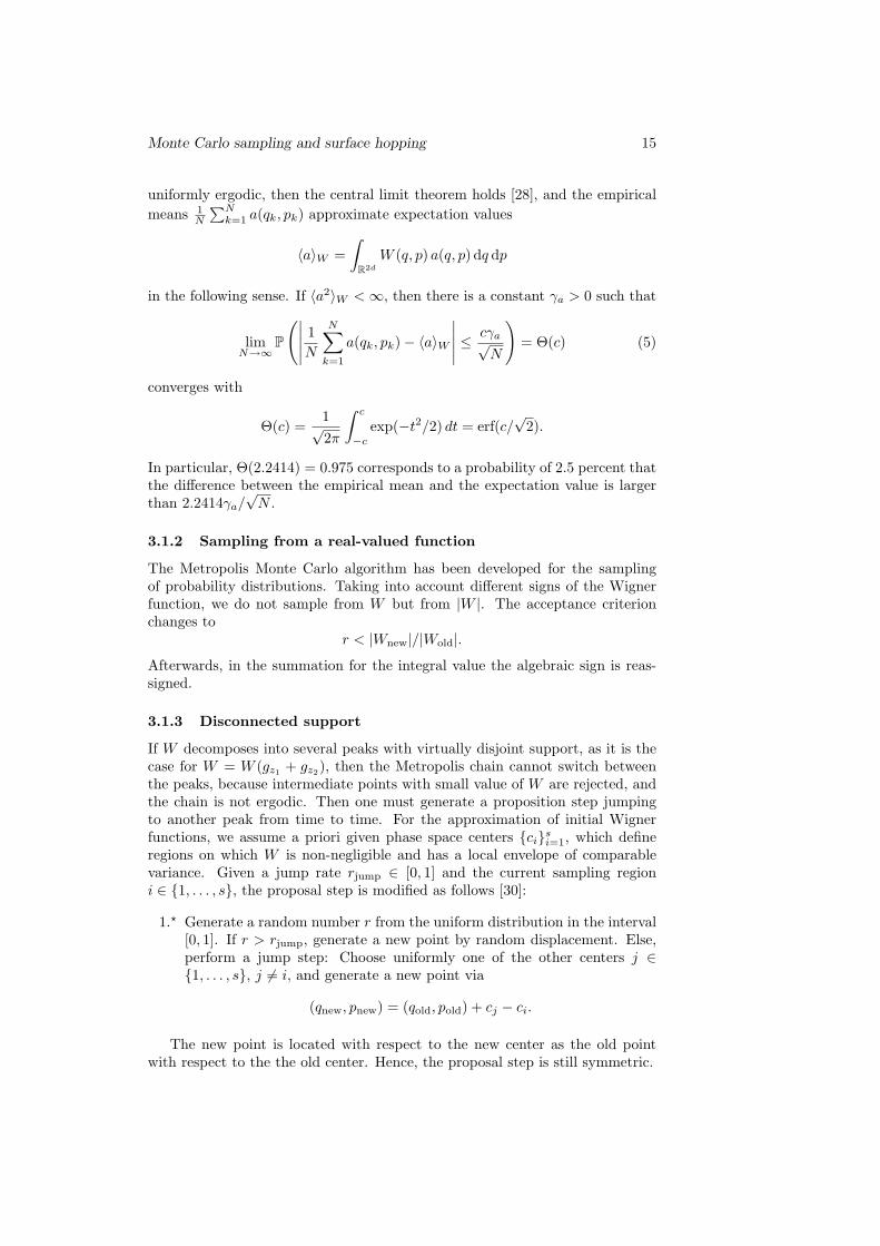
uniformly ergodic, then the central limit theorem holds [28], and the empiricalmeans 1

N

∑Nk=1 a(qk, pk) approximate expectation values

〈a〉W =∫

R2d

W (q, p) a(q, p) dq dp

in the following sense. If 〈a2〉W <∞, then there is a constant γa > 0 such that

limN→∞

P

(∣∣∣∣∣ 1N

N∑k=1

a(qk, pk)− 〈a〉W

∣∣∣∣∣ ≤ cγa√N

)= Θ(c) (5)

converges with

Θ(c) =1√2π

∫ c

−c

exp(−t2/2) dt = erf(c/√

2).

In particular, Θ(2.2414) = 0.975 corresponds to a probability of 2.5 percent thatthe difference between the empirical mean and the expectation value is largerthan 2.2414γa/

√N .

3.1.2 Sampling from a real-valued function

The Metropolis Monte Carlo algorithm has been developed for the samplingof probability distributions. Taking into account different signs of the Wignerfunction, we do not sample from W but from |W |. The acceptance criterionchanges to

r < |Wnew|/|Wold|.

Afterwards, in the summation for the integral value the algebraic sign is reas-signed.

3.1.3 Disconnected support

If W decomposes into several peaks with virtually disjoint support, as it is thecase for W = W (gz1 + gz2), then the Metropolis chain cannot switch betweenthe peaks, because intermediate points with small value of W are rejected, andthe chain is not ergodic. Then one must generate a proposition step jumpingto another peak from time to time. For the approximation of initial Wignerfunctions, we assume a priori given phase space centers cis

i=1, which defineregions on which W is non-negligible and has a local envelope of comparablevariance. Given a jump rate rjump ∈ [0, 1] and the current sampling regioni ∈ 1, . . . , s, the proposal step is modified as follows [30]:

1.? Generate a random number r from the uniform distribution in the interval[0, 1]. If r > rjump, generate a new point by random displacement. Else,perform a jump step: Choose uniformly one of the other centers j ∈1, . . . , s, j 6= i, and generate a new point via

(qnew, pnew) = (qold, pold) + cj − ci.

The new point is located with respect to the new center as the old pointwith respect to the the old center. Hence, the proposal step is still symmetric.


−50 0 50−500

50−1

−0.5

0

0.5

1

qyqx

(a) Integrand for Gaussian wavepacket.

−500

50

−50

0

500

0.2

0.4

qx

q=(0.5,0.05), p=(0,0)

qy

(b) Integrand for excited oscillatorstate.

Figure 1: Typical integrands in the computation of the Wigner function byMonte Carlo quadrature. The left and right plot show the integrands for thesingle Gaussian wave packet at (q0, p) with p = p0+(0.3, 0.3) and for the excitedoscillator state at (q0, p0), respectively.

3.2 Importance Sampling

For evaluating the Wigner function, one has to solve the d-dimensional Fourierintegral W (ψ)(q, p) =

∫Rd f(x) dx with

f(x) = (2π)−d eix·p ψ(q − ε2x)ψ(q + ε

2x).

The real part of two typical integrands f(x) is plotted in Figure 1. With con-ventional quadrature the integrand is evaluated on a grid, which does not onlyrequire a very fine resolution, but also leads to the curse of dimensionality. Mostof the computing time is spent on points, where the integrand is negligible. Tosample many points in regions where the integrand is large and few elsewhere,is the basic idea behind importance sampling.

3.2.1 Standard approach

One rewrites the integral in the form

W (ψ)(q, p) =∫

Rd

f(x)w(x)

w(x) dx,

where w(x) ≥ 0 is a positive normalized weight function,∫

Rd w(x) dx = 1. Ifone generates sampling points according to the function w(x), then the integralcan be approximated by

W (ψ)(q, p) ≈ I :=1L

L∑k=1

f(xk)w(xk)

. (6)

If the sampling points are independent and identically distributed or a uniformlyergodic Markov chain, then the central limit theorem guarantees convergenceof the empirical mean as L → ∞. The quality of the approximation cruciallydepends on the choice of the weight function w. If the sampling points are


independent and identically distributed, then I has mean µ =∫

Rd f(x) dx andvariance ⟨

(I − µ)2⟩

w=

1L

∫Rd

(f(x)w(x) − µ

)2

w(x) dx.

Hence, small variances are achieved for weight functions w, which closely resem-ble the integrand f . On the other hand, w should allow for an efficient sampling,and we have chosen a Gaussian function

w(x) = (2π)−d/2σ−dw exp

(−|x− µ|2

2σ2w

), (7)

whose mean µ ∈ Rd and standard deviation σw > 0 depend on the integrandunder consideration.

Due to the possible oscillations of the integrand, convergence might be ex-tremely slow, and we have used the following simple convergence test. Assumewe have computed M different values ImM

m=1 of the integral determiningW (ψ)(q, p). Moreover, we assume that these values are normally distributedwith mean I and variance σ2

I ,

I =1M

M∑m=1

Im, σ2I =

1M − 1

M∑m=1

(Im − I)2.

We compute a 95-percent confidence interval according to KI = ±z σI/√M

with z = 1.96. The sampling is continued until

KI < I√ε. (8)

If the tolerance is not reached within a maximum number Nmax of samplingsteps, the point (q, p) will be rejected. There are more sophisticated conver-gence criteria as for example the Gelman-Rubin criterion [5], which is not onlybased on information between different sequences but also on within-sequenceinformation. Its output is a number R > 1 which indicates how much the distri-butional estimate might improve if the simulations run longer. However, sincethe simple test yields satisfactory results, we have not explored this possibility.

3.2.2 Embedded importance sampling

If the integrand is the product of two functions, f(x) = g(x)w(x), where oneof them has a known integral Iw =

∫Rd w(x) dx and can be used as a weight

function, then the approximation (6) simplifies to

W (ψ)(q, p) ≈ 1L

1Iw

L∑k=1

g(xk),

where the points xk are distributed according to w(x). This approach usesmore information on the integrand, and the numerical experiments show thatit expectedly outperforms the standard approach.


100 200 500 1000 1500 20000

0.005

0.01

0.015

0.02

number of sampling points

(a) Convergence behavior of simpleMonte Carlo sampling for the observ-able q1(0).

0 200 400 600 800 1000 1200−0.2

−0.1

0

0.1

0.2

value of W

rela

tive

erro

r

meanRelError=0.0034, meanAbsError=0.5642, meanSamSteps=1322, meanAcc=1

(b) Distribution of errors for the integrationof the Wigner function by importance sam-pling.

Figure 2: Gaussian wave packet. The left plot illustrates the convergence be-havior of the simple Monte Carlo sampling for the observable q1(t = 0). Singlepoints show the absolute difference to the true value 0.5, while the solid curveindicates the values of cγq1/

√N with γq1 =

√ε/2 ≈ 0.07 and c = 2.2414. The

right plot gives the distribution of relative errors with respect to the exact valueof the Wigner function W for quadrature by importance sampling for N = 500phase space sampling points.

4 Gaussian wave packet

The Gaussian wave packet gz0 is one of the simplest examples for an initial wavefunction. Since its Wigner function is also Gaussian, the initial phase space sam-pling can be simplified a lot compared to the proposed strategy. Nevertheless,ignoring the analytic knowledge on the explicit form of W (gz0), we also studythe performance of the Metropolis approach.

4.1 Approximation

Since W (gz0) is a Gaussian, one can simply generate approximation points bysampling from a multi-dimensional normal distribution. This is much faster thanMetropolis Monte Carlo because the summation of the displacement vector isomitted and the acceptance ratio is equal to 1. We refer to this method as simpleMonte Carlo in the following and analyze its performance in combination withthe surface hopping algorithm. Afterwards, we forget about the Gaussian shapeand examine the choice of the displacement ∆ in the Metropolis Monte Carlomethod.

4.1.1 Simple Monte Carlo

We first sample the Gaussian Wigner function by generating points from afour-dimensional standard normal distribution and multiplying them with thestandard deviation σ =

√ε/2. Let us briefly verify the convergence rate of

order 1/√N for the observable a(q, p) = q1, as it is given by the central limit

theorem for independent identically distributed random variables. In this case,


100 200 500 1000 1500 2000

0.3

0.35

0.4

0.45

0.5

0.55

0.6

valu

es


(a) Analytic evaluation of W .

100 200 500 1000 1500 2000

0.3

0.35

0.4

0.45

0.5

0.55

0.6

valu

es


(b) Monte Carlo computation of W .

Figure 3: Gaussian wave packet. Statistics of P+(tf) for simple Monte Carloapproximation of the initial distribution. For the left and right plot the values ofthe Wigner function are determined analytically and by importance sampling,respectively. The results are compared for different numbers of sampling points(N = 100, . . . , 2000), where m = 10 runs of the single switch algorithm areevaluated for each N . The dashed horizontal line indicates the reference value0.422 from Strang splitting.

the constant γq1 = σ is the standard deviation of the random variables. Fig-ure 2(a) plots the values of the difference | 1

N

∑Nk=1 q1,k− 0.5| for ten repetitions

of the sampling with a fixed number of points N ∈ 100, . . . , 2000 as well as thereference function N 7→ cγq1/

√N with c = 2.2414. Nearly all values are below

this boundary, which should indeed be satisfied with probability Θ(c) = 0.975in the limit N →∞.

The next goal is to examine the results from the single switch algorithm forsimple Monte Carlo sampling of the initial distribution. As accuracy criterion,we take the deviation of the final population P+(tf) from the reference value0.422 stemming from the Strang splitting scheme. The sampling of the initialdistribution is performed with N = 100, . . . , 2000 different numbers of samplingpoints. Then, for each fixed N there are m = 10 runs of the surface hoppingalgorithm. The results are illustrated as boxplots in Figure 3(a). The boxes havelines at the lower quartile, median, and upper quartile values. The dashed linesextending from each end of a box show the extent of the rest of the data. Theyextend out to the most extreme data value within 1.5 times the interquartilerange of the sample. Data values beyond these lines are marked as outliers.The variances become smaller as N increases. Hence, the results of a singlerun become more reliable for larger N . Though the surface hopping algorithmsystematically overestimates the reference value, all the mean values only differby two to three percent.

4.1.2 Metropolis Monte Carlo

Investigating sampling strategies applicable for arbitrary initial distributions,we repeat the experiments from the previous paragraph with Metropolis MonteCarlo sampling. We use the algorithm explained in §3.1 with normally dis-tributed displacement ∆ ∼ σapprN4(0, 1). The starting point of the Markov


−1.2 −1 −0.8

−0.2

−0.1

0

0.1

0.2

p1

p 2

N=1000, σ=0.01

(a) σappr = 0.01

−1.2 −1 −0.8

−0.2

−0.1

0

0.1

0.2

p1

p 2

N=1000, σ=0.1

(b) σappr = 0.1

Figure 4: Gaussian wave packet. Distribution of momenta p(0) resulting fromMetropolis Monte Carlo approximation of the Wigner function with differentvalues of the standard deviation σappr of the random displacement.

Table 1: Gaussian wave packet. Mean acceptance ratios over 10 runs ofMetropolis Monte Carlo sampling with different values of the standard devi-ation σappr of the random displacement.σappr 0.01 0.05 0.1 0.2

acceptance ratio 0.9059 0.5258 0.2211 0.0033

chains is always the center z0 = (q0, p0) of the Gaussian W (gz0). In the litera-ture, see for example [25, 27], more elaborate proposal densities are discussed.However, in the following experiments the simple normal distribution yieldsquite large acceptance ratios.

The standard deviation σappr of the displacement should be comparable tothe one of the distribution to be sampled, which is σ =

√ε/2. We perform the

algorithm with a fixed number of sampling points N = 1000 and different valuesof σappr ∈ 0.1

√ε, 0.5

√ε,√ε, 2

√ε. We repeat each run ten times and analyze

the corresponding mean values. As expected, the mean acceptance ratio, thatis the number of proposed points over the number of accepted points, increaseswith smaller displacement, see Table 1. Though a high acceptance ratio isdesirable, small displacements prevent the Markov chain from quickly exploringthe complete distribution. Indeed, Figure 4 illustrates that the distribution ofp(t = 0) is more dense for σappr = 0.01 than for σappr = 0.1. Hence, we useσappr = 0.5

√ε throughout the following experiments as a compromise between

acceptance ratio and exploration of sampling space.

4.2 Integration

Standard importance sampling introduces an importance sampling function wand samples from this distribution. In general, this sampling is performed viaMetropolis Monte Carlo. However, if w is Gaussian, simple Monte Carlo isfaster. Further simplifications are possible if embedded importance sampling


can be applied. The embedded importance sampling function can be sampledvia Metropolis Monte Carlo or, if it is Gaussian, via simple Monte Carlo. In thefollowing, we compare these different approaches and use simple Monte Carlosampling for the approximation of the Wigner function.

4.2.1 Standard importance sampling

Evaluation of the Wigner function in a point (q, p) requires solving the integral

14επ3

e−1ε |q−q0|2

∫R2

cos(x · (p− p0)) e−ε4 |x|

2dx. (9)

There are oscillations with respect to x which are modulated by a Gaussianenvelope. As the distance |p−p0| gets larger the oscillation frequency increases,which causes severe difficulties in Monte Carlo quadrature. Figure 1(a) showsthe integrand for (q0, p) with p = p0 + (0.3, 0.3). Even though the integralvalue is small in this case, the quadrature scheme can yield large errors due tonumerical cancellation. We test two strategies to circumvent these difficulties.The first method introduces a cut-off for p, meaning that during the sampling ofthe Wigner function all points with |p−p0| > tolp are rejected. For the Gaussianwith variance σ =

√ε/2, the cut-off tolerance is set to tolp = 3

√ε/2 ≈ 0.21,

which includes 99.9% of the probability density. However, this requires some apriori knowledge about the distribution function, which is not always accessible.The second method uses the convergence criterion (8).

We apply importance sampling with Gaussian importance function w asdefined in (7) with µ = 0 and σw =

√2/ε, according to the variance of the

Gaussian part of the integrand, and draw from w by simple Monte Carlo sam-pling. We set the number of chains M = 5 and the maximum number of stepsNmax = 104. A typical distribution of relative errors with respect to the exactvalue of the Wigner function is illustrated in Figure 2(b). The relative as wellas the absolute error are centered around zero (mean relative error = 0.0034,mean absolute error = 0.5642), supporting the expectation that oscillations withsubsequent small integral value pose the main difficulty. If the sampled phasepoints are propagated by the single switch algorithm, then the statistics for theupper level population at time t = tf are worse than before, when the analyticvalues of the Wigner function have been used. Figure 3(b) shows the resultsfor N = 100, . . . , 2000 sampling points and m = 10 surface hopping runs foreach fixed N . The variances are larger, and the mean values differs from thereference by a few percent only for N ≥ 500.

Finally, we compare the cut-off and the multiple chain strategy by applyingthem to two points (q0, p), whose momentum component is inside and outsidethe cut-off range, that is p = p0 + (0.1, 0.1) and p = p0 + (0.3, 0.3). Theimportance function w is sampled via Metropolis Monte Carlo with randomdisplacement chosen from the normal distribution N2(0, σ2) with σ = 1

2σw. Inthe first case, the exact value is 137.12. The sampling converges after 4000steps with mean I = 148.71 and confidence bound KI = 14.5. For the secondpoint, the analytic value of the integral is 1.5 · 10−5. We obtain I = −0.5 withKI = 10.65. The sampling does not converge within the maximum number ofsteps, and the second point is rejected according to both strategies.


4.2.2 Embedded importance sampling

In general, an analytic calculation of the Wigner function is impossible but theintegrand might contain some fast decaying function whose integral is known.Using that

ε

4π

∫R2

e−ε4 |x|

2dx = 1,

the integral (9) can be evaluated via Monte Carlo quadrature as

W (gz0)(q, p) ≈1

Lε2πe−

1ε |q−q0|2

L∑k=1

cos(xk · (p− p0)). (10)

The sampling points xkLk=1 are distributed according to exp(− ε

4 |x|2), which

represents the 2-dimensional normal distribution N2(0, 2/ε).Comparing accuracy and complexity of the four different ways of importance

sampling, we calculate the Wigner function at the 2188 grid points of §2.2.1.The first method uses the importance function w from (7) with µ = 0, σw =√

2/ε and samples it via Metropolis Monte Carlo with random displacementfrom the normal distribution N2(0, σ2) with σ = 1

2σw. The second methodreplaces Metropolis Monte Carlo by directly drawing from w. The third methodapplies formula (10) and generates the quadrature points by Metropolis MonteCarlo with random displacement from N2(0, σ2). The fourth approach directlysamples from exp(− ε

4 |x|2).

The results are listed in Table 2. The relative and absolute errors refer tothe quadrature error in the computation of W (gz0)(qk, pk) and are mean valuesover all points (qk, pk)2188k=1 . All the relative errors are around one percent, whilethe absolute errors improve for simple Monte Carlo. The sampling error is thedeviation from the vector of expectation values in position and momentum z0measured in the supremum norm. It lies in the permille range. The error ofthe final population on the upper level P+(tf) is computed from this single runof the surface hopping algorithm. It is roughly two percent. Time refers tothe total amount of time to compute the Wigner function for all 2188 points.It reduces significantly for embedded importance sampling with simple MonteCarlo. The Monte Carlo steps give the number of quadrature points requiredto compute the Wigner function averaged over all grid points (qk, pk). Theacceptance ratio is the mean value over all 2188 importance sampling runs. Themass ratio is the ratio of the sum of the Wigner function at phase space points,for which the quadrature achieves the convergence criterion (8), over the sumof the Wigner function at all grid points.

5 Superposition of Gaussian wave packets

For the superposition of Gaussian wave packets the Wigner function is no longerpositive and has several peaks with disconnected support. In the following, weexamine the performance of the strategies which have been proposed in §3.

5.1 Approximation

The Wigner function consists of the sum of the two phase space Gaussians

W (gzj )(q, p) = (πε)−d exp(− 1

ε |(q, p)− zj |2), j = 1, 2


Table 2: Single Gaussian wave packet. Accuracy and complexity in the compu-tation of the Wigner function via different importance sampling schemes.

standard import. sampling embedded import. sampling

Metropolis MC Simple MC Metropolis MC Simple MC

relative error 0.012 0.009 0.013 0.009absolute error 0.473 0.031 0.438 0.153sampling error 0.0052 0.0004 0.0052 0.0011P+(tf) error 0.019 0.018 0.021 0.019time (sec) 7940 6031 3349 1960MC steps 3163 2351 3118 2370acceptance ratio 0.76 1 0.76 1mass ratio 0.88 0.94 0.86 0.95

plus an oscillatory cross term c(q, p) localized around the middle point z+ = 0,

c(q, p) = (πε)−de−|(q,p)|2/ε cos(

1ε (q, p) ∧ z−

),

which has a Gaussian envelope with the same variance and oscillates with a fre-quency proportional to the difference z− = (10

√ε,√ε,−2, 0). Consequently, we

choose the random displacement as before, namely from the normal distributionwith standard deviation σappr = 0.5

√ε. Moreover, an elaborate integration by

parts, see Theorem 7.7.1 in [10], gives a positive constant C > 0 such that forall smooth compactly supported functions a : R2d → C and all k ∈ N0∣∣∣∣∫

R2d

c(q, p)a(q, p) dq dp∣∣∣∣ ≤ Cεk

∑|α|≤k

|z−|α/2−k‖Dαa‖∞.

Thus, averages of the cross term are super-polynomially small with respect to thesemiclassical parameter, which indicates that the cross term might be neglectedwithout affecting the overall accuracy of the surface hopping algorithm.

During the sampling, jumps between the centers z1 and z2 of the two Gaus-sians and the middle point z+ are performed, if a random number r uniformlydistributed in [0, 1] is below the jump rate rjump. As expected, the larger jumprates increase the overall acceptance ratio, see Table 3. However, the final popu-lation P+(tf) of the surface hopping is rather insensitive to the rate. Figure 5(b)presents the statistics for three choices of rjump ∈ 0.2, 0.5, 0.8. For the twosmaller values rjump = 0.2, 0.5 there is more mixing within the components andconsequently no outliers, while for rjump = 0.8 there are three of them. Hence,we have fixed rjump = 0.2 for the following experiments.

As for the single Gaussian wave packet before, one observes a convergencerate of order 1/

√N for the approximation of observables via Monte Carlo sam-

pling, see Figure 5(a). Examining the influence of the initial sampling on theaccuracy of the surface hopping population P+(tf), we have considered differ-ent numbers of sampling points N = 100, . . . , 3000 and have performed thehopping algorithm m = 20 times for each fixed number of sampling points.The results are illustrated in Figure 6(a). With a few hundred sampling pointsthe mean value already differs from the reference value 0.436 by a few percent.


Table 3: Superposition of Gaussian wave packets. The acceptance ratio increaseswith growing jump rate. The ratios are mean values over 10 runs with 2000sampling points each.rjump 0.2 0.5 0.8

acceptance ratio 0.55 0.66 0.75

100 200 500 1000 1500 2000 3000 50000

0.05

0.1

0.15

0.2

0.25


σ=1

(a) Convergence behavior of MonteCarlo sampling for the observableq1(0).

0.2 0.5 0.8

0.4

0.45

0.5

0.55

valu

esjump rate

(b) Boxplots for the distribution ofP+(tf) around the exact value 0.436.

Figure 5: Superposition of Gaussian wave packets. The left plot illustrates theconvergence behavior of the sampling for the observable q1(0). Single pointsshow the absolute difference to the true value 0, while the solid curve indicatesthe values of cγq1/

√N with γq1 = 1 and c = 2.2414. The right plot shows the

final population of the upper level for three different values of the jump rate.For each jump rate, 10 runs with 2000 points each have been performed.

100 200 500 1000 1500 2000 30000.3

0.4

0.5

0.6

0.7

0.8

0.9

valu

es


(a) Complete distribution.

100 200 500 1000 1500 2000 30000.3

0.4

0.5

0.6

0.7

0.8

valu

es


(b) Distribution without oscillatorypart.

Figure 6: Superposition of Gaussian wave packets. Statistics of P+(tf) forMetropolis Monte Carlo sampling of the complete initial distribution (left handside) and without the oscillatory middle peak (right hand side). The results arefor different numbers of sampling points (N = 100, . . . , 3000), where m = 20runs of the single switch algorithm were evaluated for each N . The dashedhorizontal line indicates the reference value 0.436 from Strang splitting.


−1000 −500 0 500 1000−0.2

−0.1

0

0.1

0.2

value of W

rela

tive

erro

r

meanRelError=0.0053, meanAbsError=0.1558, meanSamSteps=1494

(a) Distribution of errors for the inte-gration of W by importance sampling.

100 200 500 1000 1500 2000

0.3

0.4

0.5

0.6

0.7

0.8

0.9

valu

es


(b) Boxplots for the distribution ofP+(tf) around the exact value 0.436.

Figure 7: Superposition of Gaussian wave packets. The left plot shows thedistribution of relative errors w.r.t. the exact value of the Wigner function for500 sampling points. The right plot shows the statistics of P+(tf) for initialMonte Carlo sampling and evaluation of the Wigner function via importancesampling. The results are compared for different numbers of sampling points(N = 100, . . . , 2000), where m = 10 runs of the single switch algorithm wereevaluated for each N .

Furthermore, with more points the results improve in the sense of variance re-duction. Hence, fewer sampling points require several simulations, whereas formany sampling points fewer simulations are sufficient to obtain reliable results.A reduction of variance is also achieved by ignoring the oscillatory middle peakof the initial distribution, see Figure 6(b). This supports the previous predic-tion that the cross term can be neglected because its contribution to integrationerrors is much more significant than its portion w.r.t. the phase space density.

5.2 Integration

Now, we also compute the Wigner function via importance sampling. The twointegrals defining the Wigner functions W (gz1) and W (gz2) have already beendealt with in the previous section §4.2. The integrals occurring for the oscillatorycross term c(q, p) ∫

R2cos(x · (p− p+)) e−

12 x·q− e−

ε4 |x|

2dx

are only slightly different due to the additional term e−12 x·q− . We apply standard

importance sampling with a Gaussian proposal distribution w of mean µ = 0and standard deviation σw =

√2/ε, where the quadrature points are directly

drawn from w. For each phase space point (q, p) we use M = 5 different chainsof maximal length Nmax = 104.

There are the same two regimes observed for the single Gaussian wave packet.If the distance of (q, p) to the middle center z+ = 0 is sufficiently large, then theintegrand is dominated by oscillations, and the point is rejected if the conver-gence criterion (8) is not met. If (q, p) is close enough to z+, then the integrandis a regular function with bell-shaped envelope, and the quadrature achieves


Table 4: Superposition of Gaussian wave packets. Final level population fordifferent values of ε, different phase space representations (Wigner or Husimi),and different sampling strategies (grid based or MCMC). The reference valueis calculated with a highly resolved Strang splitting. The particle numbersfrom the grid based sampling are given in parentheses, while the Monte Carlosampling always uses 5000 points.ε 10−1 10−2 10−3 5 · 10−4

1. reference value 0.37798 0.43565 0.52582 0.54363

2. Husimi (grid) 0.5095 0.5371 0.6037 0.6149(4754) (6170) (5548) (5394)

3. Wigner (coarse grid) 0.3372 0.4054 0.5299 0.5079(5108) (5024) (2920) (4811)

4. Wigner (fine grid) 0.3856 0.4397 0.5268 0.4613(31163) (55799) (6302) (11743)

5. Husimi (MCMC) 0.5031 0.5379 0.6221 0.63966. Wigner (MCMC) 0.3963 0.4385 0.5692 0.59567. Wigner (MCMC, no middle part) 0.3876 0.4375 0.5404 0.5585

the expected accuracy. Indeed, for 500 phase points the quadrature producesa mean relative and mean absolute error with respect to the exact value of theWigner function, which is of size 0.0053 and 0.1558, respectively. The meanchain length to achieve convergence is 1494, and the mean acceptance ratio forphase space points is 0.9. Figure 7(a) illustrates the corresponding distributionof relative errors, which again are largest for small values of the Wigner function.

Also the results of the single switch algorithm have the same tendencies asbefore. Sampling the initial Wigner function with different numbers of samplingpoints N = 100, . . . , 2000 and computing the function value via importancesampling, Figure 7(b) shows larger variances than for the experiments withanalytic function values, but also the expected variance reduction for a growingnumber of initial phase space points.

5.3 Approximation of the Husimi function

Now we explore the performance of the single switch algorithm, when the Wignerfunction of the initial wave function is replaced by the Husimi function. Whilethe semiclassical parameter is set to ε ∈ 0.0005, 0.001, 0.01, 0.1, the two differ-ent phase functions are sampled in a grid based way or by the previous MonteCarlo method. As for the Wigner function, the Metropolis Monte Carlo sam-pling of the Husimi function is rather insensitive to the variance of the randomdisplacement, and we fix for both functions σappr = 0.5

√ε.

Let us first consider the grid based results, see Table 4, lines two to four.For the Husimi function, the number of grid points and hence the number ofparticles is increased until the final population P+(tf) converges up to an errorof roughly one percent. Such behavior already occurs for moderate particlenumbers around N = 5000. For the Wigner function, the same grids do notyield convergence, and one has to refine significantly. For small semiclassical


10−3 10−2 10−10

0.05

0.1

ε

diffe

renc

e in

leve

l pop

ulat

ion

HusimiWignerWigner with many particlesMCMC HusimiMCMC WignerMCMC Wigner without middle part

Figure 8: Superposition of Gaussian wave packets. The semilogarithmic plotshows the error in the final level population P+(tf) for the Husimi and Wignerfunction with varying value of ε. The first three curves are based on grid basedsampling, while the last three ones result from MCMC sampling.

parameter ε = 0.0005 convergence is not obtained, since a reasonably sizeduniform grid cannot resolve the rapid oscillations of the middle peak. However,the population errors for the converged sampling of the Wigner function areroughly three times smaller than those for the Husimi function, see also Figure 8.This difference can be explained by the better asymptotic properties of theWigner function with respect to classical transport. As discussed in section §1.2,the Egorov theorem for scalar Schrodinger equations gives an approximationerror of order ε2 for the Wigner function, whereas the Husimi function onlyyields an error of order ε. The rougher approximation of the single switchalgorithm does not bury this difference.

The Monte Carlo results all use N = 5000 sampling points and are the meanvalues of ten different runs, see Table 4, lines five to seven. The outcome forthe Husimi function changes only slightly. The results are a bit better for largersemiclassical parameters and worse for small values. The Monte Carlo sampledWigner function without oscillatory middle peak achieves the smallest error,which differs from those for the Husimi function by roughly a factor three.

6 Excited harmonic oscillator state

The Wigner function of the excited harmonic oscillator state e is a Gaussian ofvariance ε/2 multiplied with an even quadratic polynomial attaining negativevalues for small momenta,

W (e)(q, p) =4 e−

1ε |(q−q0,p)|2

ε4π2(11)( ∏

j=1,2

(qj − q0,j)2 +∑

(j,k)=(1,2),(2,1)

(qj − q0,j)2(p2k − ε

2 ) +∏

j=1,2

(p2j − ε

2 )).


100 200 500 1000 1500 20000

0.05

0.1

0.15

0.2

0.25


σ=1

(a) Convergence behavior of MonteCarlo sampling for the observableq1(0).

−400 −200 0 200−0.2

−0.1

0

0.1

0.2

value of W

rela

tive

erro

r

meanRelError=0.0011, meanAbsError=−0.2836, meanSamSteps=2294

(b) Distribution of errors for the inte-gration of W by importance sampling.

Figure 9: Excited oscillator state. The left plot illustrates the convergencebehavior of Monte Carlo sampling for the observable q1(0), when the analyticexpression of the Wigner function W is used. Single points show the absolutedifference to the true value 0.5, while the solid curve indicates the values ofcγq1/

√N with γq1 = 1 and c = 2.2414. The right plot shows the distribution of

relative errors w.r.t. the exact value of W for 500 sampling points.

At first, we use the analytic expression for the Wigner function and sample fromthis distribution via Metropolis Monte Carlo with random displacement

∆ ∼ N4(0, σ2appr), σappr = 0.5

√ε.

The error in the computation of the position expectation value in the firstcomponent q1(0) again decreases as 1/

√N , see Figure 9(a). The results for the

final population on the upper level obtained by the surface hopping algorithmare illustrated in Figure 10(a). As in the previous examples, the error decreasesdown to a few percent, if the number of sampling points is large enough. Hence,the approximation is not affected by the negative values of the Wigner function.

The integrals for the computation of the Wigner function W (e)(q, p) are∫R2

cos(x · p)(q21 − ε2

4 x21

)(q22 − ε2

4 x22

)e−

ε4 |x|

2dx.

Their integrand differs from those for the Gaussian wave packets by a polynomialterm. A typical integrand is illustrated in Figure 1(b). There are oscillations,but they are moderate as long as the momentum p is small and the magnitudeof W (e)(q, p) large enough. We apply embedded importance sampling withrespect to x 7→ exp(− ε

4 |x|2) and use simple Monte Carlo to sample from this

proposal function. For each integral, there are M = 5 chains of maximal lengthNmax = 104 stopped by the convergence criterion (8). Figure 9(b) shows therelative errors for 500 phase space points. As for the Gaussian wave packets, theerrors are bounded by 0.2. The mean relative and absolute errors are 0.0011 and−0.2836, respectively. The mean chain length is 2294, hence somewhat largerthan the length 1494 obtained in the Gaussian case. The mean acceptance ratiois about 0.7 and smaller than the previously observed 0.9. In clear contrast tothe Gaussian wave packets, there is no direct relationship between the errors


100 200 500 1000 1500 2000−0.2

0

0.2

0.4

0.6

0.8

valu

es


(a) Analytic evaluation of W .

100 200 500 1000 1500 2000−0.2

0

0.2

0.4

0.6

0.8

valu

es


(b) Monte Carlo computation of W .

Figure 10: Excited oscillator state. Statistics of P+(tf) for Metropolis MonteCarlo sampling of the initial distribution with analytic evaluation and MonteCarlo computation of the Wigner function. The results are compared for differ-ent numbers of sampling points (N = 100, . . . , 2000), where m = 10 runs of thesingle switch algorithm were evaluated for each N . The dashed horizontal lineindicates the reference value 0.571 from Strang splitting.

and the magnitude of the Wigner function, since the polynomial factor of theintegrand causes a modulation of the envelope function, which in turn prolongsthe mixing time of the Markov chain and generates errors dominating those dueto high frequency oscillations. However, as before, the results for the upper levelpopulation obtained by a subsequent surface hopping nicely converge for largerparticle numbers; see Figure 10(b).

Conclusion

We have addressed the Monte Carlo sampling of Wigner functions, as it arisesin the context of particle methods for Schrodinger equations in the semiclassicalregime. The sampling poses an approximation and a quadrature problem. Forboth we have considered a Monte Carlo approach, motivated by the followingobservations. Quantum molecular dynamics is typically formulated on high-dimensional configuration spaces. The potential of Schrodinger equations fornuclear propagation is mostly determined with coarse resolution, since its valuefor each nuclear configuration is based on the solution of a high-dimensionalelectronic structure problem. Moreover, also particle methods for Wigner func-tions in the spirit of an Egorov theorem are asymptotic approximations withrather coarse accuracy as well.

For the approximation problem we have proposed and tested an adaptionof the Metropolis Monte Carlo algorithm to real-valued functions with discon-nected support. The algorithm requires a priori physical knowledge on thefunctional support of the Wigner function, in the sense that phase space points,which specify the different components, are used as an input. The methodenforces random jumps between the regions, within which the same local pro-posal steps generate the chain. While the construction of jump proposal stepswith high acceptance ratio is a challenging task in classical molecular dynamics


simulations, the similarities between the jump regions ensured the success ofthis approach in our examples. In the numerical experiments we have observedconvergence of computed observables with an error of order 1/

√N , where N is

the number of sampling points, as it is implied by the central limit theorem forergodic Markov chains.

For the integration problem, which arises when evaluating the Wigner func-tion, we have tested the performance of importance sampling with Gaussianweight function. For certain phase space points, the quadrature problem is ill-conditioned due to a highly oscillatory integrand. For the considered test cases,however, these points are characterized by small values of the Wigner functionand can thus be neglected. The proposed simple convergence criterion, which isbased on the variance between different sampling chains, is able to detect suchpoints.

We have demonstrated in three sets of numerical experiments that the pro-posed Monte Carlo approach to the sampling of Wigner functions yields surfacehopping results, which reach an accuracy comparable to the one obtained by aconverged grid-based sampling with analytic evaluation of the Wigner function.We have also considered the Husimi function as an alternative phase space repre-sentation, since it is non-negative and less oscillatory. However, the subsequentsurface hopping results are systematically less accurate than for the Wignerfunction, which can be explained by the different order of approximation errorin the Egorov theorem for scalar Schrodinger equations.

The presented numerical experiments are low-dimensional, since we haveaimed at a combination of initial Monte Carlo sampling with surface hoppingand its validation against a reliable solution of the underlying Schrodinger sys-tems. Such a comparison is naturally bound to a few degrees of freedom. High-dimensional experiments as well as the Monte Carlo integration of oscillatoryfunctions with stationary points have to be addressed in future work.

A Reference solutions

For evaluating the different initial sampling strategies in combination with thesingle switch algorithm, we directly solve the Schrodinger system with a pseudo-spectral Strang splitting scheme. For this two-dimensional problem a spacediscretization based on the fast Fourier transform and an operator splitting withthird order local convergence in time [13] provides accurate reference solutions.The number of time steps is set to 5000 for all experiments. The length of thetime interval allows the wave function to pass the crossing point once. The finaltime is tf = 10

√ε for the Gaussians and tf = 20

√ε for the excited harmonic

oscillator state.Table 5 contains the computational domains, the grid sizes, the final pop-

ulation P+(tf) and the achieved accuracy. The accuracy of the solution refersto the difference ‖ψ(tf) − ψc(tf)‖L2 of the final reference solution ψ(tf) and acoarser solution ψc(tf), which is computed with fourth the number of grid pointsand half the number of time steps. In section §5.3, we varied the semiclassicalparameter ε to compare Wigner and Husimi functions. The input parametersas well as the accuracy of the corresponding reference solutions are listed inTable 6. The achieved errors are all sufficient for the validation of the singleswitch algorithm, whose accuracy for the computation of quadratic quantities


Table 5: Input parameters and results for the reference solution if ε = 0.01.

domain fine grid size P+(tf) accuracy

Gaussian wave packet [−2, 2]× [−1, 1] 1024× 512 0.422 4.7 · 10−7

Superposition [− 32 ,

32 ]× [− 3

4 ,34 ] 2048× 1024 0.436 1.9 · 10−4

Excited oscillator [−4, 4]× [−2, 2] 2048× 1024 0.571 5.2 · 10−4

Table 6: Input parameters and results for the reference solution in case of thesuperposition of two Gaussians in dependence on the semiclassical parameter ε.

ε domain fine grid size P+(tf) accuracy

10−1 [−10, 10]× [−5, 5] 2048× 1024 0.378 1.0 · 10−3

10−2 [− 32 ,

32 ]× [− 3

4 ,34 ] 2048× 1024 0.436 1.9 · 10−4

10−3 [−1, 1]× [− 12 ,

12 ] 2048× 1024 0.526 1.6 · 10−7

5 · 10−4 [− 12 ,

12 ]× [− 1

4 ,14 ] 2048× 1024 0.544 1.0 · 10−7

of the wave function typically varied around three percent.

B Analytical Wigner transformation

For the cross term of the Wigner function W (gz1 + gz2), one solves the integral

W (gz1 , gz2)(q, p) = (2π)−d

∫Rd

eix·p gz1(q − ε2x)gz2

(q + ε2x) dx

= (2π)−d(πε)−d/2∫Rd

eix·p e−12ε (|q− ε

2 x−q1|2+|q+ ε2 x−q2|2) e

iε (p1·(q− ε

2 x−q1)−p2·(q+ ε2 x−q2)) dx,

where q1,2 and p1,2 denote the position and momentum component of the phasespace points z1,2 for the rest of the calculation. Rewriting the quadratic part as

|q − ε2x− q1|2 + |q + ε

2x− q2|2 = |q − q1|2 + |q − q2|2 + ε2

2 |x|2 + εx · q−,

one has

W (gz1 , gz2)(q, p) = (2π)−d(πε)−d/2 e−12ε |q−q1|2− 1

2ε |q−q2|2

eiε (p1·(q−q1)−p2·(q−q2))

∫Rd

eix·(p−p++ i2 q−) e−

ε4 |x|

2dx. (12)

One uses the value of the Gaussian integral∫R

eiywe−αy2dy =

√πα e−w2/(4α), w ∈ C, α > 0

for wj = pj − pj+ + i

2qj− with j = 1, . . . , d and α = ε/4. Since

d∑j=1

(wj)2 = |p− p+|2 − 14 |q−|

2 + i(p− p+) · q−,


one gets

W (gz1 , gz2)(q, p) = (πε)−d e−12ε |q−q1|2− 1

2ε |q−q2|2 eiε (p1·(q−q1)−p2·(q−q2))

e−1ε |p−p+|2e

14ε |q−|

2e−

iε (p−p+)·q− .

Observing that − 12 |q − q1|2 − 1

2 |q − q2|2 + 14 |q−|

2 = −|q − q+|2 and

p1 · (q − q1)− p2 · (q − q2)− (p− p+) · q− = ((q, p)− z+) ∧ z− − p+ · q−

one arrives at

W (gz1 , gz2)(q, p) = (πε)−d e−iε p+·q− e−

1ε |(q,p)−z+|2 e

iε ((q,p)−z+)∧z− .

and

c(q, p) = 12 (W (gz1 , gz2)(q, p) +W (gz2 , gz1)(q, p))

= (πε)−d e−1ε |(q,p)−z+|2 cos

(1ε (p+ · q− − ((q, p)− z+) ∧ z−)

)Finally we compute the Wigner function for the two-dimensional excited oscil-lator state e(q) for the case q0 = (0, 0). The defining integral

W (e)(q, p) = (επ)−3

∫R2

eix·p(q21 − ε2

4 x21)(q

22 − ε2

4 x22) e−

1ε |q|

2− ε4 |x|

2dx

falls into four parts, whose value can be determined due to∫R

eiywy2 e−αy2dy = −

√π

4 α−5/2(w2 − 2α) e−w24α , w ∈ C, α > 0.

With α = ε4 and w = pj for j = 1, 2, one obtains∫R2

eix·p e−ε4 |x|

2dx = 4π

ε e−1ε |p|

2,∫

R2eix·px2

1 e−ε4 |x|

2dx =

∫R

eix1p1x21 e−

ε4 x2

1 dx1

∫R

eix2p2 e−ε4 x2

2 dx2,

= −8√πε−5/2(p2

1 − ε2 ) e−

1ε p2

1

√4πε e−

1ε p2

2

= − 16πε3 (p2

1 − ε2 ) e−

1ε |p|

2,∫

R2eix·px2

2 e−ε4 |x|

2dx = − 16π

ε3 (p22 − ε

2 ) e−1ε |p|

2,∫

R2eix·px2

1x22 e−

ε4 |x|

2dx =

∏j=1,2

∫R

eixjpjx2j e−

ε4 x2

j dxj

=∏

j=1,2 − 8√πε−5/2(p2

j − ε2 ) e−

1ε p2

j

= 64πε5 (p2

1 − ε2 )(p2

2 − ε2 ) e−

1ε |p|

2.

Hence,

W (e)(q, p) =

4 e−1ε |(q,p)|2

ε4π2

(q21q

22 + q22(p2

1 − ε2 ) + q21(p2

2 − ε2 ) +

∏j=1,2(p

2j − ε

2 )).


C Position densities by density estimation

At some final time t = tf > 0 the single switch algorithm produces two sets ofirregularly spaced points

(q±k , p±k ) ∈ R2d | k = 1, . . . ,M±

with associated weights w±k , which approximate the value of the Wigner func-tions W (ψ±(tf)) in these points. A simple approximation in arbitrary phasespace points (q?, p?) can be deduced by kernel density estimation [21]

W (ψ±(tf))(q?, p?) ≈ 1M±

M±∑k=1

w±k K((q?, p?)− (qk, pk))

with Gaussian kernel

K : R2d → R, x 7→ (π/c)−d exp(−c|x|2).

Let p1, . . . , pN ⊂ Rd be a grid in momentum space with uniform patch sizeω(p1) = . . . = ω(pN ). Then, the position densities in a point q? ∈ Rd areapproximately

|ψ±(tf , q?)|2 =∫

Rd

W (ψ±(tf))(q?, p) dp

≈ 1M±

N∑j=1

M±∑k=1

w±k K((q?, pj)− (qk, pk))ω(pj).

We use this approach for a visual comparison of the position densities ob-tained from Strang splitting with the approximation resulting from surface hop-ping with Monte Carlo quadrature. The obtained plots have been insensitivewith respect to the variation of c in the interval [10, 50]. Choosing c = 20,Figures 11, 12, and 13, collect the densities for the single Gaussian wave packet,the superposition of two Gaussians, and the excited oscillator state, respec-tively. One observes a good agreement between the mean positions, however,as expected, no pointwise agreement, since the surface hopping approximationof the Wigner function only holds in a weak sense.

References[1] N. de Bruijn. Uncertainty principles in Fourier analysis. In O. Shisha, editor, Inequalities,

pages 57–71. Academic Press, 1967.

[2] W. Domcke, D. Yarkony, and H. Koppel, editors. Conical intersections. World Scientific,Singapore, 2004.

[3] G. Folland. Harmonic Analysis in Phase Space. Princeton University Press, Princeton,1989.

[4] D. Frenkel and B. Smit. Understanding Molecular Simulation – From Algorithms toApplications, volume 1 of Computational Science Series. Academic Press, 2002.

[5] A. Gelman and D. B. Rubin. Inference from iterative simulation using multiple sequences.Statistical Sience, 7:457–511, 1992.

[6] G. Granucci and M. Persico. Critical appraisal of the fewest switches algorithm for surfacehopping. J. Chem Phys., 126:134114, 2007.


qx

q y−1.5 −1 −0.5 0

−0.5

0

0.5

(a) Strang: |ψ+(q, tf)|2

qx

q y

−1.5 −1 −0.5 0

−0.5

0

0.5

(b) SH: |ψ+(q, tf)|2

qx

q y

−1.5 −1 −0.5 0

−0.5

0

0.5

(c) Strang: |ψ−(q, tf)|2

qx

q y

−1.5 −1 −0.5 0

−0.5

0

0.5

(d) SH: |ψ−(q, tf)|2

Figure 11: Gaussian wave packet. Position density of the upper and lower levelfunctions |ψ+(q, t)|2 and |ψ−(q, t)|2 at time t = tf . The figures on the left showthe results from Strang splitting, the figures on the right the results from asingle surface hopping run with 1000 sampling points.

qx

q y

−1 0 1

−1

−0.5

0

0.5

1


qx

q y

−1 0 1

−1

−0.5

0

0.5

1

(b) SH: |ψ+(q, tf)|2

qx

q y

−1 0 1

−1

−0.5

0

0.5

1


qx

q y

−1 0 1

−1

−0.5

0

0.5

1

(d) SH: |ψ−(q, tf)|2

Figure 12: Superposition of Gaussian wave packets. Position density of theupper and lower level function |ψ+(q, t)|2 and |ψ−(q, t)|2 at time t = tf . Thefigures on the left show the results from Strang splitting, the figures on the rightthe results from a single surface hopping run with 1000 sampling points, whichdoes not properly reflect the symmetries between the two peaks.


qx

q y

−3 −2 −1 0−1.5

−1

−0.5

0

0.5

1

1.5


qx

q y

−3 −2 −1 0−1.5

−1

−0.5

0

0.5

1

1.5

(b) SH: |ψ+(q, tf)|2

qx

q y

−3 −2 −1 0−1.5

−1

−0.5

0

0.5

1

1.5


qx

q y

−3 −2 −1 0−1.5

−1

−0.5

0

0.5

1

1.5

(d) SH: |ψ−(q, tf)|2

Figure 13: Excited oscillator state. Position density of the upper and lowerlevel function |ψ+(q, t)|2 and |ψ−(q, t)|2 at time t = tf . The figures on the leftshow the results from Strang splitting, the figures on the right the results froma single surface hopping run with 1000 sampling points.

[7] K. Grochenig. Foundations of Time-Frequency Analysis. Birkhauser, Boston, 2001.

[8] W. K. Hastings. Monte Carlo sampling methods using Markov chains and their applica-tions. Biometrika, 57:97–109, 1970.

[9] E. Heller. Wigner phase space method: analysis for semiclassical applications. J. ChemPhys., 65:1289–1298, 1976.

[10] L. Hormander. The Analysis of Linear Partial Differential Operators I. Springer-Verlag,Berlin, 1983.

[11] K. Husimi. Some formal properties of the density matrix. Proc. Phys. Math. Soc. Japan,22:264–314, 1940.

[12] D. Iagolnitzer. Microlocal essential support of a distribution and decomposition theorems- an introduction. In F. Pham, editor, Hyperfunctions and Theoretical Physics, pages121–132. Springer, New York, 1975.

[13] T. Jahnke and C. Lubich. Error bounds for exponential operator splitting. BIT,40(4):735–744, 2000.

[14] C. Fermanian Kammerer and C. Lasser. Propagation through generic level crossings: asurface hopping semigroup. SIAM J. Math. An., 2008.

[15] C. Lasser, T. Swart, and S. Teufel. Construction and validation of a rigorous surfacehopping algorithm for conical crossings. Comm. Math. Sci., 2007.

[16] C. Lasser and S. Teufel. Propagation through conical crossings: an asymptotic semigroup.Comm. Pure Appl. Math, 58:1188–1230, 2005.

[17] A. Martinez. An Introduction to Semiclassical and Microlocal Analysis. Springer, NewYork, 2002.

[18] N. Metropolis, A. W. Rosenbluth, M. N. Rosenbluth, A. H. Teller, and E. Teller. Equationof state calculations by fast computing machines. J. Chem. Phys., 21(6):1087–1092, 1953.

[19] J. Moyal. Quantum mechanics as a statistical theory. Proc. Cambridge Philos. Soc.,45:99–124, 1949.


[20] E. Novak. Is there a curse of dimension for integration? In C.-H. Lai, P. E. Bjorstad,M. Crss, and O. B. Widlund, editors, Eleventh Int. Conf. on Domain DecompositionMethods, pages 88–95. Domain Decomposition Press, Bergen, 1999.

[21] E. Parzen. On estimation of a probability density function and mode. Ann. Math. Stat.,33:1065–1076, 1962.

[22] P. H. Peskun. Optimum Monte Carlo sampling using Markov chains. Biometrika, 60:607–612, 1973.

[23] L. Plaskota, K. Ritter, and G. W. Wasilkowski. Average case complexity of weightedapproximation and integration over Rd with isotropic weight. In K.T. Fang, F.J. Hicker-nell, and H. Niederreiter, editors, Monte Carlo and Quasi Monte Carlo Methods 2000,pages 479–522. Springer, 2002.

[24] D. Robert. Autour de l’Approximation Semi-Classique. Birkhauser, Boston, 1987.

[25] C. P. Roberts and G. Casella. Monte Carlo Statistical Methods. Springer, New York,1999.

[26] J. Rust. Using randomization to break the curse of dimensionality. Econometrica,65(3):487–516, 1997.

[27] A. M. Stuart, J. Voss, and P. Wiberg. Conditional path sampling of SDEs and theLangevin MCMC method. Comm. Math. Sci., 2:685–697, 2004.

[28] L. Tierney. Markov chains for exploring posterior distributions. The Annals of Statistics,22:1701–1728, 1994.

[29] J. Ville. Theory and applications of the notion of complex signal. Rept. T-92, The RandCorp., Santa Monica, California, 1958.

[30] L. Walter and M. Weber. ConfJump: a fast biomolecular sampling method which drillstunnels through high mountains. ZIB-Report 06-26, Zuse Institute Berlin, 2006. http:

//www.zib.de/Publications/abstracts/ZR-06-26/.

[31] E. Wigner. On the quantum correction for thermodynamic equilibrium. Phys. Rev.,40:749–759, 1932.

Date post:	11-Mar-2019
Category:	Documents
Upload:	vuongcong
View:	217 times
Download:	0 times

Monte Carlo sampling of Wigner functions and surface ... · Monte Carlo sampling of Wigner...

Documents