Monte Carlo Simulation of Monte Carlo Simulation of Liquid WaterLiquid Water

Daniel ShoemakerDaniel ShoemakerReza ToghraeeReza Toghraee

MSE 485/PHYS 466 - Spring 2006MSE 485/PHYS 466 - Spring 2006

ObjectiveObjective

Write a MC liquid water simulation Write a MC liquid water simulation program from scratch which yields program from scratch which yields observables that are consistent with those observables that are consistent with those found in the literature.found in the literature.

We chose to code in We chose to code in C++ since it is C++ since it is modular and object-modular and object-oriented.oriented.

The first decision we The first decision we needed to make was needed to make was which water potential which water potential to use.to use.

PotentialsPotentials

Many potentials exist for 2- 3- 4- and 5-site Many potentials exist for 2- 3- 4- and 5-site models of water.models of water.

We chose a 3-site NVT model to maintain We chose a 3-site NVT model to maintain simplicity while keeping good agreement simplicity while keeping good agreement with physical parameters.with physical parameters.

TIP3P potential:TIP3P potential: rrOH OH = 0.96 Å= 0.96 Å HOH angle = 104.52°HOH angle = 104.52° qqOO = -2q = -2qHH = -0.834, charges located directly on = -0.834, charges located directly on

atomsatoms LJLJAA = 582x10 = 582x1033 kcal Å kcal Å1212/mol, LJ/mol, LJCC = 595 kcal Å = 595 kcal Å66/mol/mol

6OO

C12OO

Amon

i

non

j ij

2ji

mn r

LJ

r

LJ

r

eqqE

Code LayoutCode Layout HeadersHeaders

Main.hMain.h MC.hMC.h

SourceSource Main.cxxMain.cxx Coordinates.cxCoordinates.cx

xx Energy.cxxEnergy.cxx GofR.cxxGofR.cxx MC.cxxMC.cxx MCMove.cxxMCMove.cxx RandGen.cxxRandGen.cxx

Necessary inputs:Necessary inputs: Number of moleculesNumber of molecules TemperatureTemperature Potential (TIP3P)Potential (TIP3P) Initialization stepsInitialization steps MC stepsMC steps How often to sample Energy How often to sample Energy

and g(r)and g(r)

Volume calculated Volume calculated automatically from automatically from densitydensity

We used standard Intel We used standard Intel and Microsoft math and Microsoft math libraries and compilers.libraries and compilers.

AlgorithmAlgorithm

Metropolis Monte Carlo algorithm:Metropolis Monte Carlo algorithm: Move random particle by a random distanceMove random particle by a random distance Calculate ∆ECalculate ∆E Accept or reject move based on -1/kTAccept or reject move based on -1/kT Update positionUpdate position

Our maximum movement length is 0.15Å to Our maximum movement length is 0.15Å to achieve an acceptance ratio between 43% achieve an acceptance ratio between 43% and 64%, depending on the number of and 64%, depending on the number of iterations.iterations.

Energy data is output every 1K-10K Energy data is output every 1K-10K iterations, with g(r) data recorded about as iterations, with g(r) data recorded about as often.often.

OptimizationOptimization

Defining H positions without trig functionsDefining H positions without trig functions Use linear algebra with properly generated Use linear algebra with properly generated

random numbers to position the H atoms based random numbers to position the H atoms based on Oon O

No lookup tables (trig functions) are usedNo lookup tables (trig functions) are used Periodic Boundary ConditionsPeriodic Boundary Conditions

Setting up a 3x3x3 matrix of boxes that surround Setting up a 3x3x3 matrix of boxes that surround the core box is a quick way to find the shortest the core box is a quick way to find the shortest distance between to particles in PBC.distance between to particles in PBC.

Much faster than subtracting Much faster than subtracting nint(distance/box)*box from the distancesnint(distance/box)*box from the distances

Energy TrendsEnergy Trends

Simulations were run with 10K Simulations were run with 10K initialization steps to ensure that the initialization steps to ensure that the energy had settled.energy had settled.

Iterations (x10)

2-D Hydrogen Binding Energy3-D Potential Energies

< Coulombic > = -0.918 +/- 0.015< Lennard-Jones > = -1.53 +/- 0.12< H binding > = -2.45 +/- 0.11

Iterations (x105)

Radial Distribution Radial Distribution FunctionFunction

g(r) does have a large initial peak, and a g(r) does have a large initial peak, and a forbidden zone near r = 0, but its dimensions do forbidden zone near r = 0, but its dimensions do not agree with theorynot agree with theory

0

0.1

0.2

0.3

0.4

0.5

0.6

0.7

0.8

0 0.5 1 1.5 2 2.5 3 3.5 4

Radius (Angstroms)

Pair

Cor

rela

tion

Func

tion

g(r)

Jorgensen et al Our Simulation

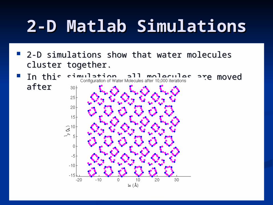
2-D Matlab Simulations2-D Matlab Simulations 2-D simulations show that water molecules cluster 2-D simulations show that water molecules cluster

together.together. In this simulation, all molecules are moved after In this simulation, all molecules are moved after

every step.every step.

ConclusionsConclusions

Our program is a fast and intuitive way to Our program is a fast and intuitive way to simulate water using Monte Carlo.simulate water using Monte Carlo.

This code can easily handle a 3-site This code can easily handle a 3-site potential, and minor modifications would potential, and minor modifications would allow 4-sites.allow 4-sites.

Our Lennard-Jones interactions are a little Our Lennard-Jones interactions are a little too strong, but the potentials behave as too strong, but the potentials behave as expected.expected.

The g(r) normalization should be The g(r) normalization should be examined to correct its scale.examined to correct its scale.

ReferencesReferences

2-D Simulations by Jihan Kim2-D Simulations by Jihan Kim

Berendsen, H. J. C. et al, Berendsen, H. J. C. et al, Intermolecular Intermolecular ForcesForces, (D. Reidel Co., Holland 1983), 331., (D. Reidel Co., Holland 1983), 331.

Frenkel, D. and B. Smit, Frenkel, D. and B. Smit, Understanding Understanding Molecular SimulationMolecular Simulation, (2, (2ndnd Ed., Academic Press Ed., Academic Press 2002).2002).

Jorgensen, W. L., Jorgensen, W. L., J. Am. Chem. Soc.J. Am. Chem. Soc. 103103, 1981, , 1981, 335.335.

Jorgensen, W. L. et al, Jorgensen, W. L. et al, J. Chem. Phys.J. Chem. Phys. 7979 (2), 12 (2), 12 July 1983, 926.July 1983, 926.

McDonald, I. R., McDonald, I. R., Mol. Phys.Mol. Phys. 2323, 1972, 41., 1972, 41.