127
Monte Carlo simulations and error analysis Matthias Troyer, ETH Zürich

Monte Carlo simulationsand error analysis
Matthias Troyer, ETH Zürich

Outline of the lecture
1. Monte Carlo integration2. Generating random numbers3. The Metropolis algorithm4. Monte Carlo error analysis5. Cluster updates and Wang-Landau sampling6. The negative sign problem in quantum Monte Carlo

1. Monte Carlo Integration

Integrating a function• Convert the integral to a discrete sum
• Higher order integrators:• Trapezoidal rule:
• Simpson rule:
f (x)dxa
b
! =b " aN
f a + ib " aN
#
$
%
& i=1
N
' + O(1/N)
f (x)dxa
b
! =b " aN
1
2f (a) + f a + i
b " aN
#
$
%
& i=1
N "1
' +1
2f (b)
#
$ (
%
& ) + O(1/N
2)
f (x)dxa
b
! =b " a3N
f (a) + (3" ("1)i) f a + ib " aN
#
$
%
& i=1
N "1
' + f (b)#
$ (
%
& ) + O(1/N
4)

High dimensional integrals• Simpson rule with M points per dimension
• one dimension the error is O(M-4 )
• d dimensions we need N = Md pointsthe error is order O(M-4 ) = O(N-4/d )
• An order - n scheme in 1 dimensionis order - n/d d in d dimensions!
• In a statistical mechanics model with N particles we have 6N-dimensional integrals (3N positions and 3N momenta).
• Integration becomes extremely inefficient!
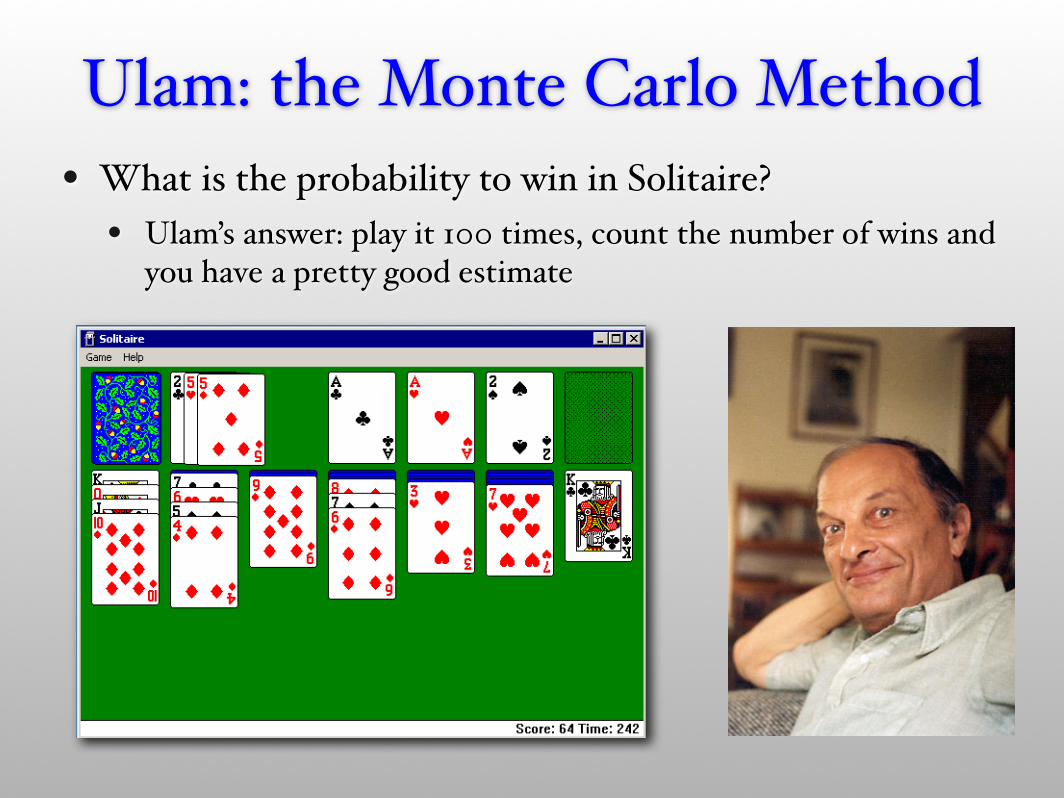
• What is the probability to win in Solitaire?• Ulam’s answer: play it 100 times, count the number of wins and
you have a pretty good estimate
Ulam: the Monte Carlo Method
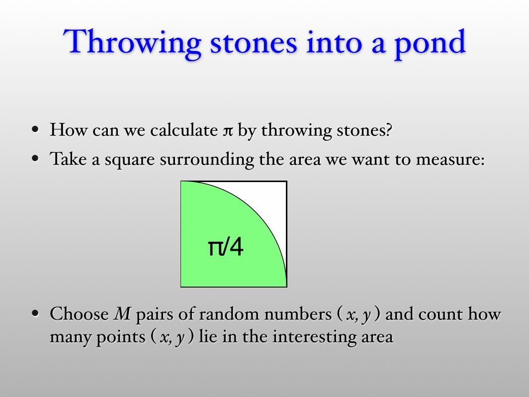
Throwing stones into a pond
• How can we calculate π by throwing stones?• Take a square surrounding the area we want to measure:
• Choose M pairs of random numbers ( x, y ) and count how many points ( x, y ) lie in the interesting area
π/4
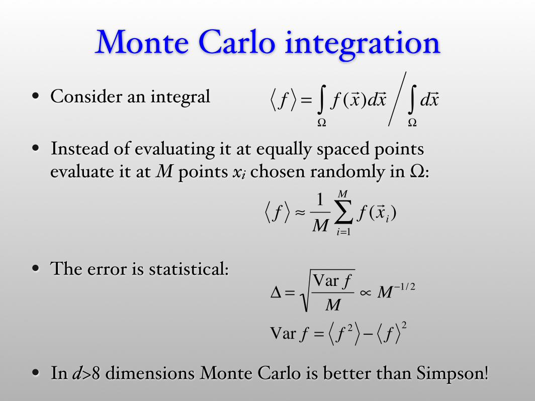
Monte Carlo integration• Consider an integral
• Instead of evaluating it at equally spaced points evaluate it at M points xi chosen randomly in Ω:
• The error is statistical:
• In d>8 dimensions Monte Carlo is better than Simpson!
f = f (! x )d! x
!
" d! x
!
"
f !1
Mf (! x i)
i=1
M
"
! =Var f
M" M
#1/ 2
Var f = f2# f
2
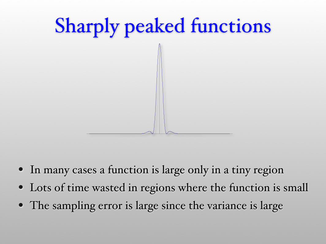
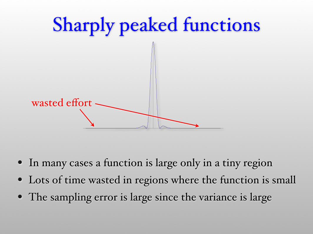
Sharply peaked functions
• In many cases a function is large only in a tiny region• Lots of time wasted in regions where the function is small• The sampling error is large since the variance is large
Sharply peaked functions
• In many cases a function is large only in a tiny region• Lots of time wasted in regions where the function is small• The sampling error is large since the variance is large
wasted effort
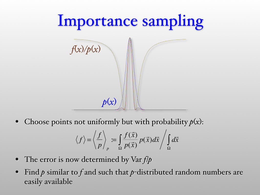
Importance sampling
• Choose points not uniformly but with probability p(x):
• The error is now determined by Var f/p• Find p similar to f and such that p-distributed random numbers are
easily available
f =f
pp
:=f (! x )
p(! x )
p(! x )d! x
!
" d! x
!
"
p(x)
f(x)/p(x)
2. Generating Random Numbers

Random numbers• Real random numbers are hard to obtain
• classical chaos (atmospheric noise)• quantum mechanics
http://www.idquantique.com/

Random numbers• Real random numbers are hard to obtain
• classical chaos (atmospheric noise)• quantum mechanics
• Commercial products: quantum random number generators• based on photons and semi-transparent mirror• 4 Mbit/s from a USB device, too slow for most MC simulations
http://www.idquantique.com/
Pseudo Random numbers
Pseudo Random numbers
• Are generated by an algorithm
Pseudo Random numbers
• Are generated by an algorithm
• Not random at all, but completely deterministic
Pseudo Random numbers
• Are generated by an algorithm
• Not random at all, but completely deterministic
• Look nearly random however when algorithm is not known and may be good enough for our purposes
Pseudo Random numbers
• Are generated by an algorithm
• Not random at all, but completely deterministic
• Look nearly random however when algorithm is not known and may be good enough for our purposes
• Never trust pseudo random numbers however!

Linear congruential generators• are of the simple form xn+1=f(xn)• A good choice is the GGL generator
with a = 16807, c = 0, m = 231-1• quality depends sensitively on a,c,m
• Periodicity is a problem with such 32-bit generators• The sequence repeats identically after 231-1 iterations• With 500 million numbers per second that is just 4 seconds!• Should not be used anymore!
xn +1 = (axn + c)modm

Lagged Fibonacci generators
• Good choices are • (607,273,+)• (2281,1252,+)• (9689,5502,+)• (44497,23463,+)
• Seed blocks usually generated by linear congruential• Has very long periods since large block of seeds• A very fast generator: vectorizes and pipelines very well
xn = xn− p ⊗ xn− qmodm
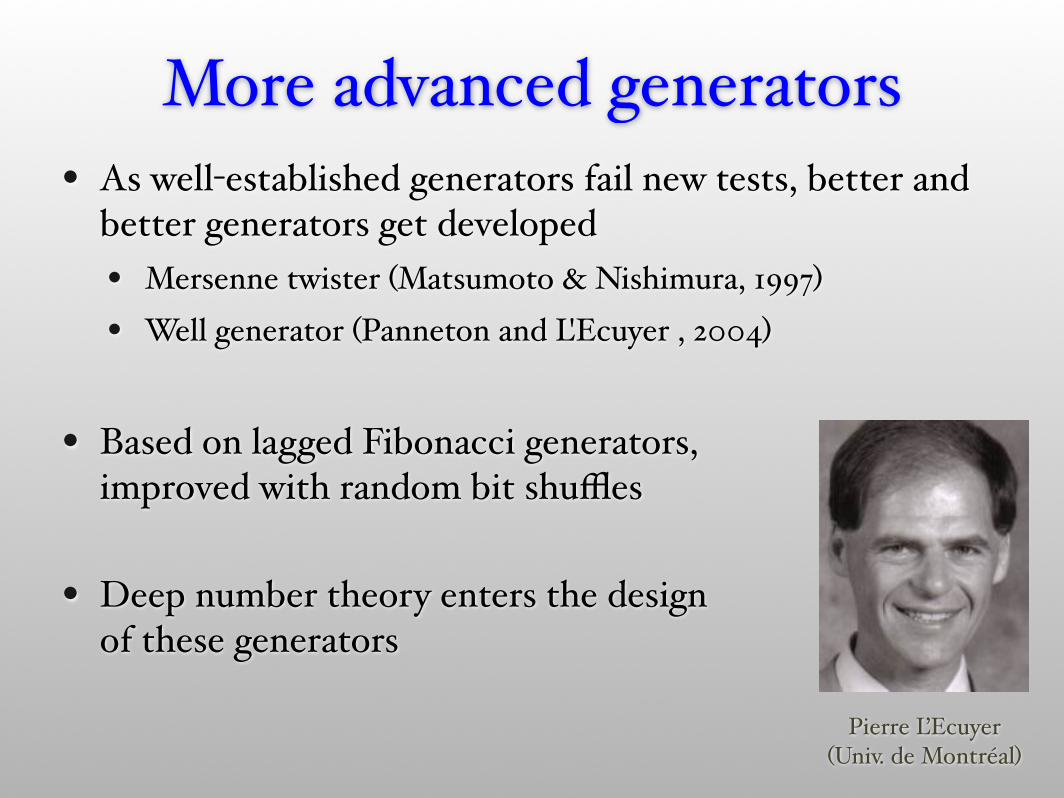
More advanced generators• As well-established generators fail new tests, better and
better generators get developed• Mersenne twister (Matsumoto & Nishimura, 1997)• Well generator (Panneton and L'Ecuyer , 2004)
• Based on lagged Fibonacci generators,improved with random bit shuffles
• Deep number theory enters the designof these generators
Pierre L’Ecuyer(Univ. de Montréal)
Are these numbers really random?
Are these numbers really random?• No!

Are these numbers really random?• No!
• Are they random enough?• Maybe?

Are these numbers really random?• No!
• Are they random enough?• Maybe?
• Statistical tests for distribution and correlations
Are these numbers really random?• No!
• Are they random enough?• Maybe?
• Statistical tests for distribution and correlations
• Are these tests enough?• No! Your calculation could depend in a subtle way on hidden
correlations!

Are these numbers really random?• No!
• Are they random enough?• Maybe?
• Statistical tests for distribution and correlations
• Are these tests enough?• No! Your calculation could depend in a subtle way on hidden
correlations!
• What is the ultimate test?• Run your simulation with various random number generators and
compare the results

Marsaglia’s diehard tests
• Birthday spacings: Choose random points on a large interval. The spacings between the points should be asymptotically Poisson distributed. The name is based on the birthday paradox.
• Overlapping permutations: Analyze sequences of five consecutive random numbers. The 120 possible orderings should occur with statistically equal probability.
• Ranks of matrices: Select some number of bits from some number of random numbers to form a matrix over 0,1, then determine the rank of the matrix. Count the ranks.
• Monkey tests: Treat sequences of some number of bits as "words". Count the overlapping words in a stream. The number of "words" that don't appear should follow a known distribution. The name is based on the infinite monkey theorem.
• Count the 1s: Count the 1 bits in each of either successive or chosen bytes. Convert the counts to "letters", and count the occurrences of five-letter "words".
• Parking lot test: Randomly place unit circles in a 100 x 100 square. If the circle overlaps an existing one, try again. After 12,000 tries, the number of successfully "parked" circles should follow a certain normal distribution.
Marsaglia’s diehard tests (cont.)
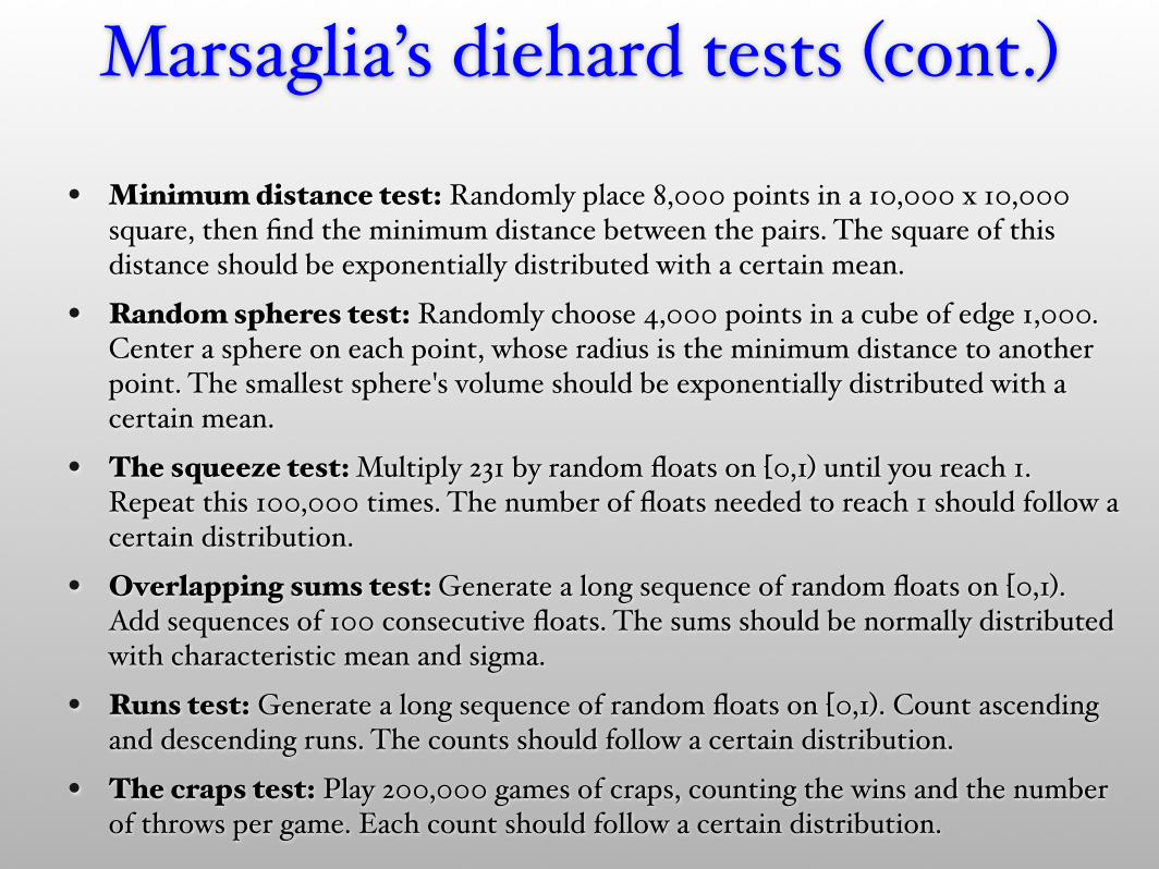
• Minimum distance test: Randomly place 8,000 points in a 10,000 x 10,000 square, then find the minimum distance between the pairs. The square of this distance should be exponentially distributed with a certain mean.
• Random spheres test: Randomly choose 4,000 points in a cube of edge 1,000. Center a sphere on each point, whose radius is the minimum distance to another point. The smallest sphere's volume should be exponentially distributed with a certain mean.
• The squeeze test: Multiply 231 by random floats on [0,1) until you reach 1. Repeat this 100,000 times. The number of floats needed to reach 1 should follow a certain distribution.
• Overlapping sums test: Generate a long sequence of random floats on [0,1). Add sequences of 100 consecutive floats. The sums should be normally distributed with characteristic mean and sigma.
• Runs test: Generate a long sequence of random floats on [0,1). Count ascending and descending runs. The counts should follow a certain distribution.
• The craps test: Play 200,000 games of craps, counting the wins and the number of throws per game. Each count should follow a certain distribution.
Non-uniform random numbers
• we found ways to generate pseudo random numbers u in the interval [0,1[
• How do we get other uniform distributions?• uniform x in [a,b[: x = a+(b-a) u
• Other distributions:• Inversion of integrated distribution • Rejection method
Non-uniform distributions
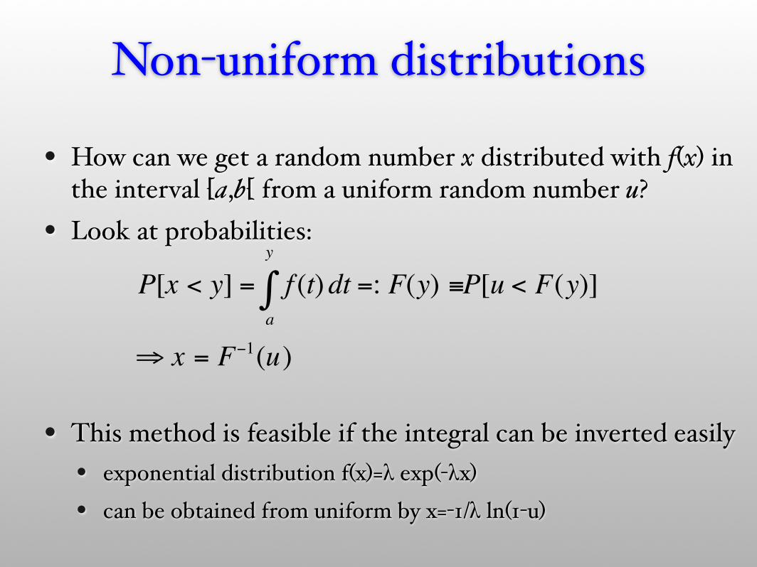
• How can we get a random number x distributed with f(x) in the interval [a,b[ from a uniform random number u?
• Look at probabilities:
• This method is feasible if the integral can be inverted easily• exponential distribution f(x)=λ exp(-λx)• can be obtained from uniform by x=-1/λ ln(1-u)
P[x < y] = f (t)dt =: F(y) ≡a
y
∫ P[u < F(y)]
⇒ x = F−1(u)
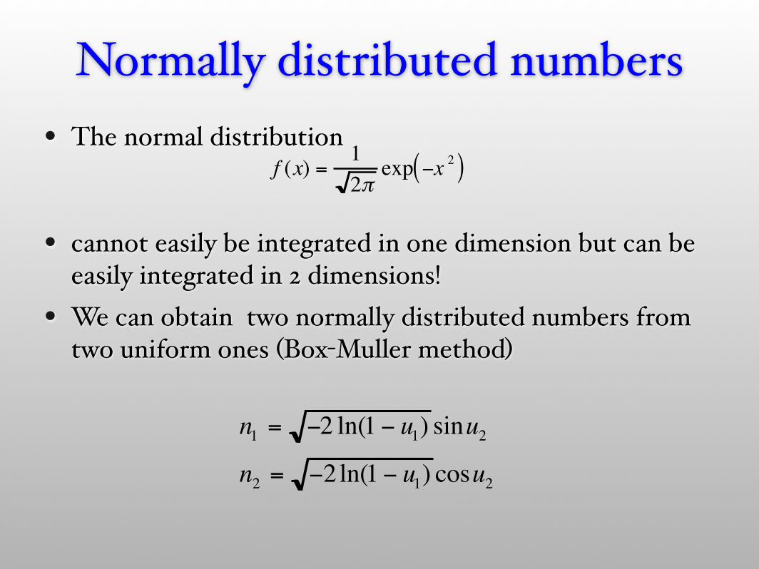
Normally distributed numbers• The normal distribution
• cannot easily be integrated in one dimension but can be easily integrated in 2 dimensions!
• We can obtain two normally distributed numbers from two uniform ones (Box-Muller method)
f (x) = 12πexp −x 2( )
n1 = −2 ln(1 − u1) sinu2n2 = −2 ln(1 − u1) cosu2

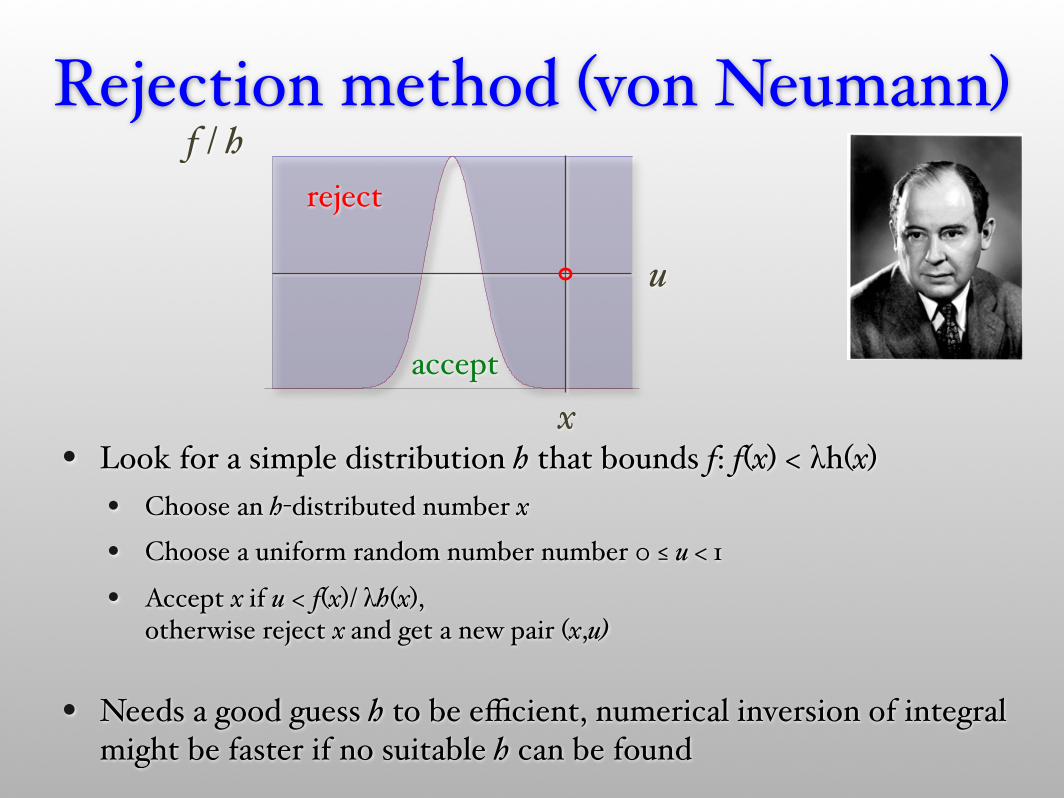
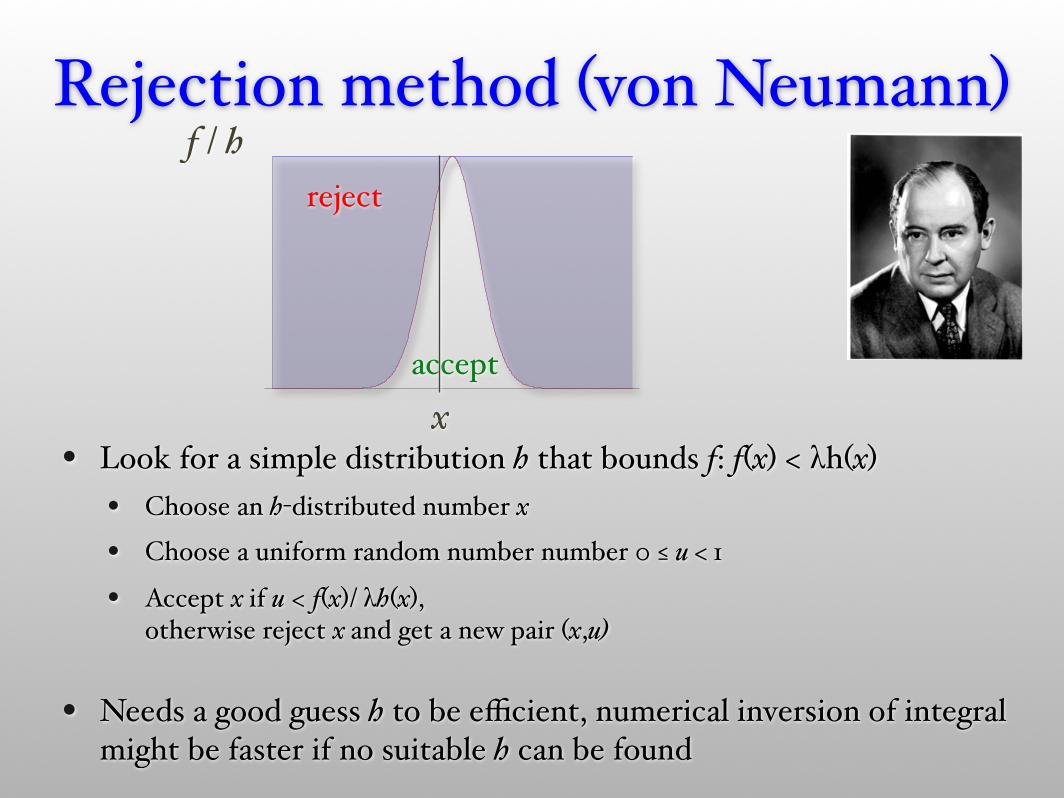
Rejection method (von Neumann)
• Look for a simple distribution h that bounds f: f(x) < λh(x)• Choose an h-distributed number x
• Choose a uniform random number number 0 ≤ u < 1
• Accept x if u < f(x)/ λh(x), otherwise reject x and get a new pair (x,u)
• Needs a good guess h to be efficient, numerical inversion of integral might be faster if no suitable h can be found
f / hreject
accept

Rejection method (von Neumann)
• Look for a simple distribution h that bounds f: f(x) < λh(x)• Choose an h-distributed number x
• Choose a uniform random number number 0 ≤ u < 1
• Accept x if u < f(x)/ λh(x), otherwise reject x and get a new pair (x,u)
• Needs a good guess h to be efficient, numerical inversion of integral might be faster if no suitable h can be found
f / h
x
reject
accept
u

Rejection method (von Neumann)
• Look for a simple distribution h that bounds f: f(x) < λh(x)• Choose an h-distributed number x
• Choose a uniform random number number 0 ≤ u < 1
• Accept x if u < f(x)/ λh(x), otherwise reject x and get a new pair (x,u)
• Needs a good guess h to be efficient, numerical inversion of integral might be faster if no suitable h can be found
f / hreject
accept
Rejection method (von Neumann)
• Look for a simple distribution h that bounds f: f(x) < λh(x)• Choose an h-distributed number x
• Choose a uniform random number number 0 ≤ u < 1
• Accept x if u < f(x)/ λh(x), otherwise reject x and get a new pair (x,u)
• Needs a good guess h to be efficient, numerical inversion of integral might be faster if no suitable h can be found
f / hreject
acceptx
u

3. The Metropolis Algorithm
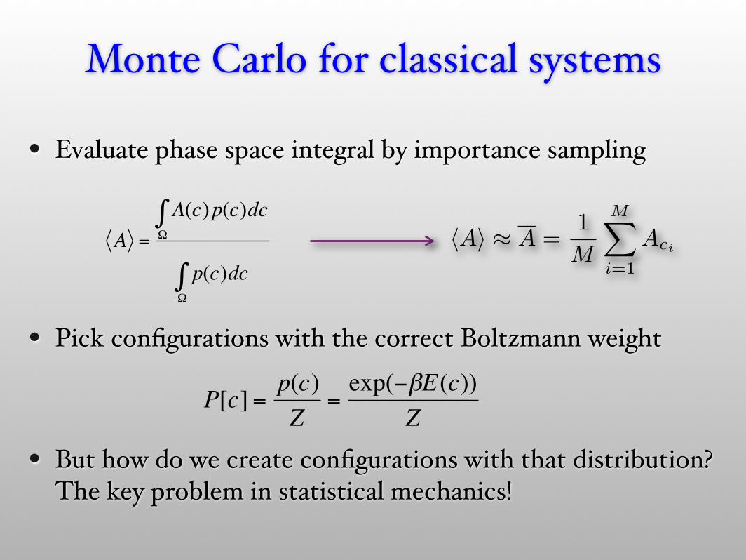
• Evaluate phase space integral by importance sampling
• Pick configurations with the correct Boltzmann weight
• But how do we create configurations with that distribution?The key problem in statistical mechanics!
Monte Carlo for classical systems
!A" # A =1M
M!
i=1
Aci
€
A =
A(c)p(c)dcΩ∫
p(c)dcΩ∫
€
P[c] =p(c)Z
=exp(−βE(c))
Z

G U E S T E D I T O R S ’
I N T R O D U C T I O N
the Top
• Metropolis Algorithm for Monte Carlo• Simplex Method for Linear Programming• Krylov Subspace Iteration Methods• The Decompositional Approach to Matrix
Computations• The Fortran Optimizing Compiler• QR Algorithm for Computing Eigenvalues• Quicksort Algorithm for Sorting• Fast Fourier Transform• Integer Relation Detection• Fast Multipole Method
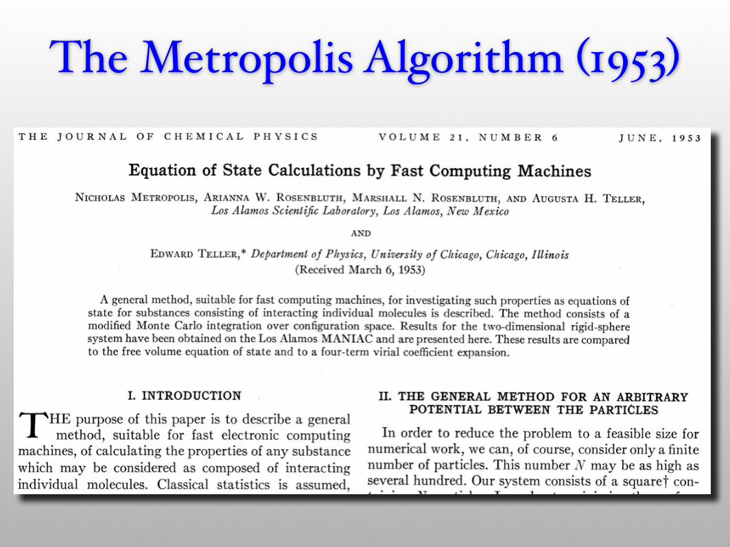
The Metropolis Algorithm (1953)
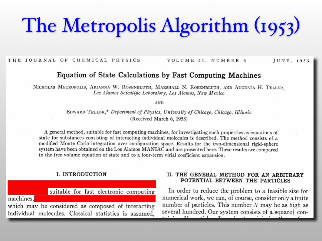
The Metropolis Algorithm (1953)

• Instead of drawing independent samples ci we build a Markov chain
• Transition probabilities Wx,y for transition x → y need to satisfy:
• Normalization:
• Ergodicity: any configuration reachable from any other
• Balance: the distribution should be stationary
• Detailed balance is sufficient but not necessary for balance
Markov chain Monte Carlo
€
c1→ c2 → ...→ ci → ci+1→ ...
€
∀x,y ∃n : W n( )x,y≠ 0
€
Wx,yy∑ = 1
€
0 =ddtp(x) = p(y)Wy,x
y∑ − p(x)Wx,y
y∑ ⇒ p(x) = p(y)Wy,x
y∑
€
Wx,y
Wy,x
=p(y)p(x)

• Teller’s proposal was to use rejection sampling:
• Propose a change with an a-priori proposal rate Ax,y
• Accept the proposal with a probability Px,y
• The total transition rate is Wx,y =Ax,y Px,y
• The choice
satisfies detailed balance and was first proposed by Metropolis et al
The Metropolis algorithm
€
Px,y= min 1,Ay,x p(y)Ax,y p(x)
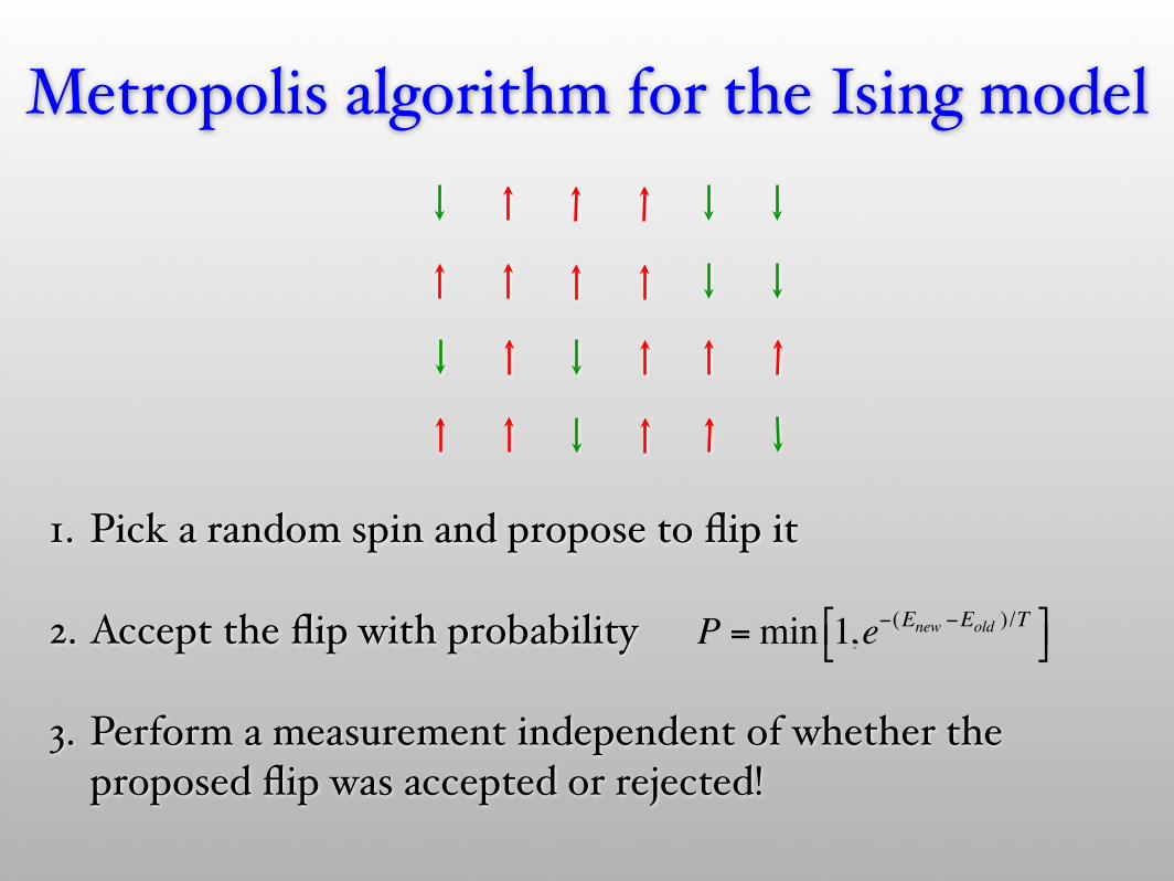
1. Pick a random spin and propose to flip it
2. Accept the flip with probability
3. Perform a measurement independent of whether the proposed flip was accepted or rejected!
Metropolis algorithm for the Ising model
P =min 1,e−(Enew −Eold )/T
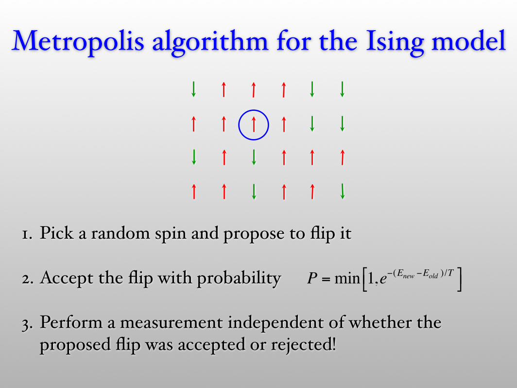
1. Pick a random spin and propose to flip it
2. Accept the flip with probability
3. Perform a measurement independent of whether the proposed flip was accepted or rejected!
Metropolis algorithm for the Ising model
P =min 1,e−(Enew −Eold )/T
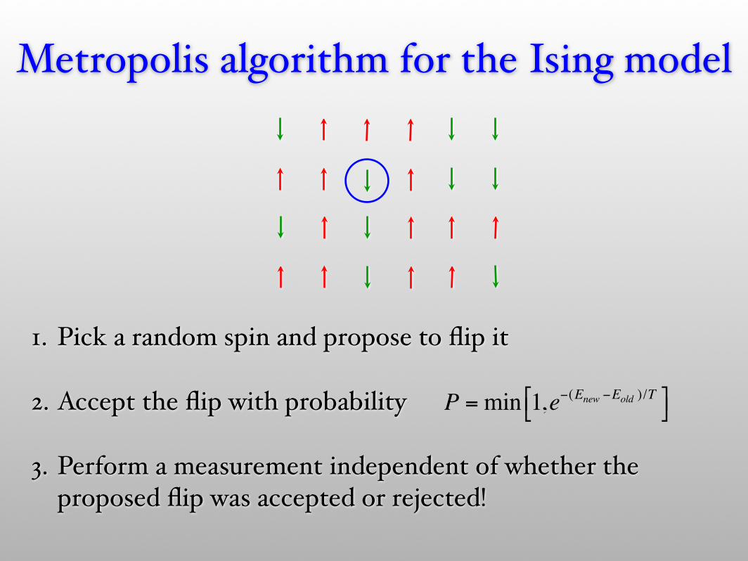
1. Pick a random spin and propose to flip it
2. Accept the flip with probability
3. Perform a measurement independent of whether the proposed flip was accepted or rejected!
Metropolis algorithm for the Ising model
P =min 1,e−(Enew −Eold )/T
Equilibration
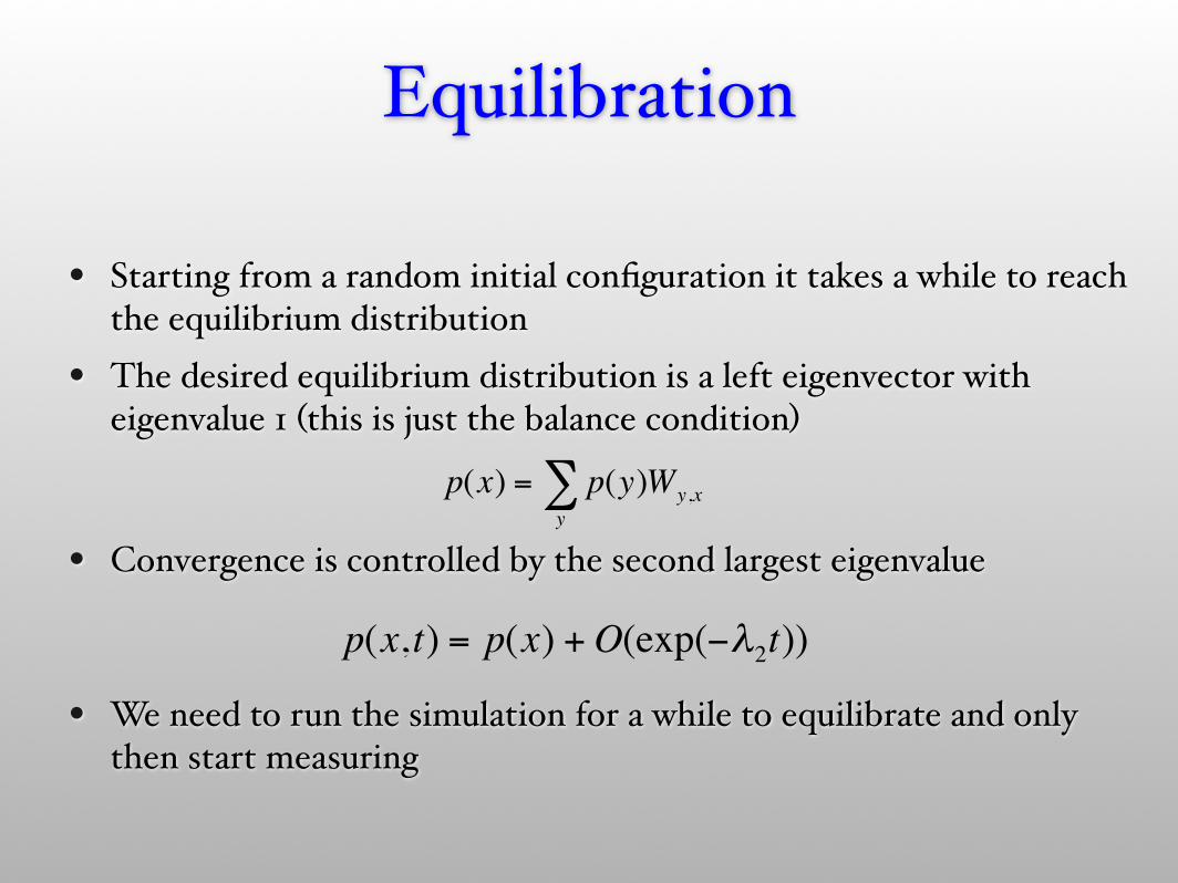
• Starting from a random initial configuration it takes a while to reach the equilibrium distribution
• The desired equilibrium distribution is a left eigenvector with eigenvalue 1 (this is just the balance condition)
• Convergence is controlled by the second largest eigenvalue
• We need to run the simulation for a while to equilibrate and only then start measuring
€
p(x, t) = p(x) +O(exp(−λ2t))€
p(x) = p(y)Wy,xy∑

4. Monte Carlo Error Analysis

Monte Carlo error analysis• The simple formula
is valid only for independent samples
• The Metropolis algorithm gives us correlated samples!The number of independent samples is reduced
• The autocorrelation time is defined by
€
ΔA =Var AM
€
ΔA =Var AM
1+ 2τA( )
€
τA =Ai+ t Ai − A 2( )
t=1
∞
∑Var A

Binning analysis• Take averages of consecutive measurements: averages become less
correlated and naive error estimates converge to real error
A1 A2 A3 A4 A5 A6 A7 A8 A9 A10 A11 A12 A13 A14 A15 A16
€
Ai(l ) =
12A2i−1( l−1) + A2i
l( )A1(1) A2
(1) A3(1) A4
(1) A5(1) A6
(1) A7(1) A8
(1)
A1(2) A2
(2) A3(2) A4
(2)
A1(3) A2
(3)
€
Δ(l ) = Var A( l ) M (l ) l→∞ → Δ = (1+ 2τA )Var A M
τA = liml→∞
122lVar A(l )
Var A(0)−1
0
0.0005
0.001
0.0015
0.002
0.0025
0.003
0.0035
0.004
0 2 4 6 8 10
L = 4L = 48
Δ(l)
binning level l
a smart implementation needs only O(log(N)) memory for N measurements
converged
not converged

Seeing convergence in ALPS• Look at the ALPS output in the first hands-on session
• 48 x 48 Ising model at the critical point
• local updates:
• cluster updates:

Correlated quantities
• How do we calculate the errors of functions of correlated measurements?
• specific heat
• Binder cumulant ratio
• The naïve way of assuming uncorrelated errors is wrong!• It is not even enough to calculate all crosscorrelations due
to nonlinearities except if the errors are tiny!
€
cV =E 2 − E 2
T 2
€
U =m4
m2 2

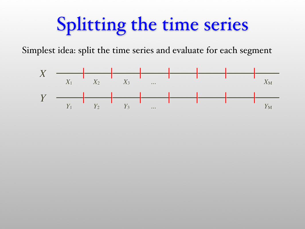
Splitting the time seriesSimplest idea: split the time series and evaluate for each segment
X
Y
Splitting the time seriesSimplest idea: split the time series and evaluate for each segment
X
YX1 X2 X3 ... XM
Y1 Y2 Y3 ... YM
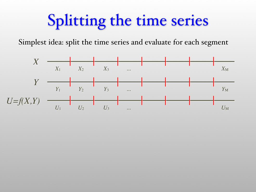
Splitting the time seriesSimplest idea: split the time series and evaluate for each segment
X
YX1 X2 X3 ... XM
Y1 Y2 Y3 ... YM
U=f(X,Y)U1 U2 U3 ... UM
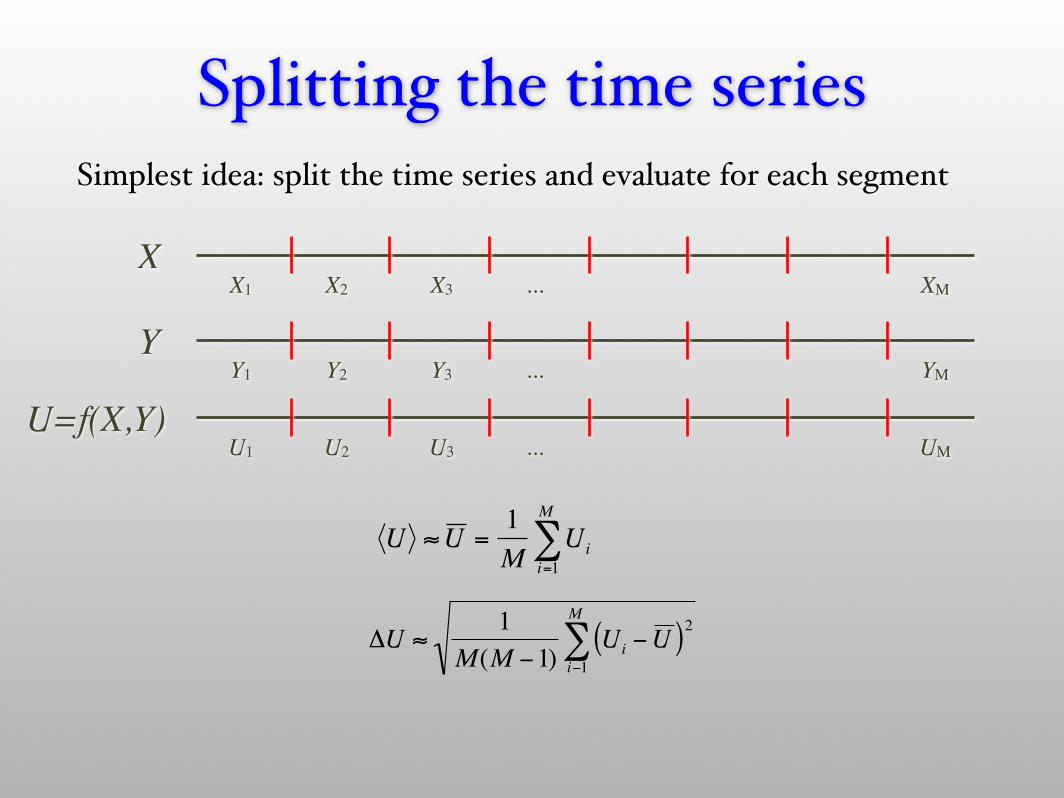
Splitting the time seriesSimplest idea: split the time series and evaluate for each segment
X
YX1 X2 X3 ... XM
Y1 Y2 Y3 ... YM
U=f(X,Y)U1 U2 U3 ... UM
€
U ≈U =1M
Uii=1
M
∑
€
ΔU ≈1
M(M −1)Ui −U ( )2
i−1
M
∑
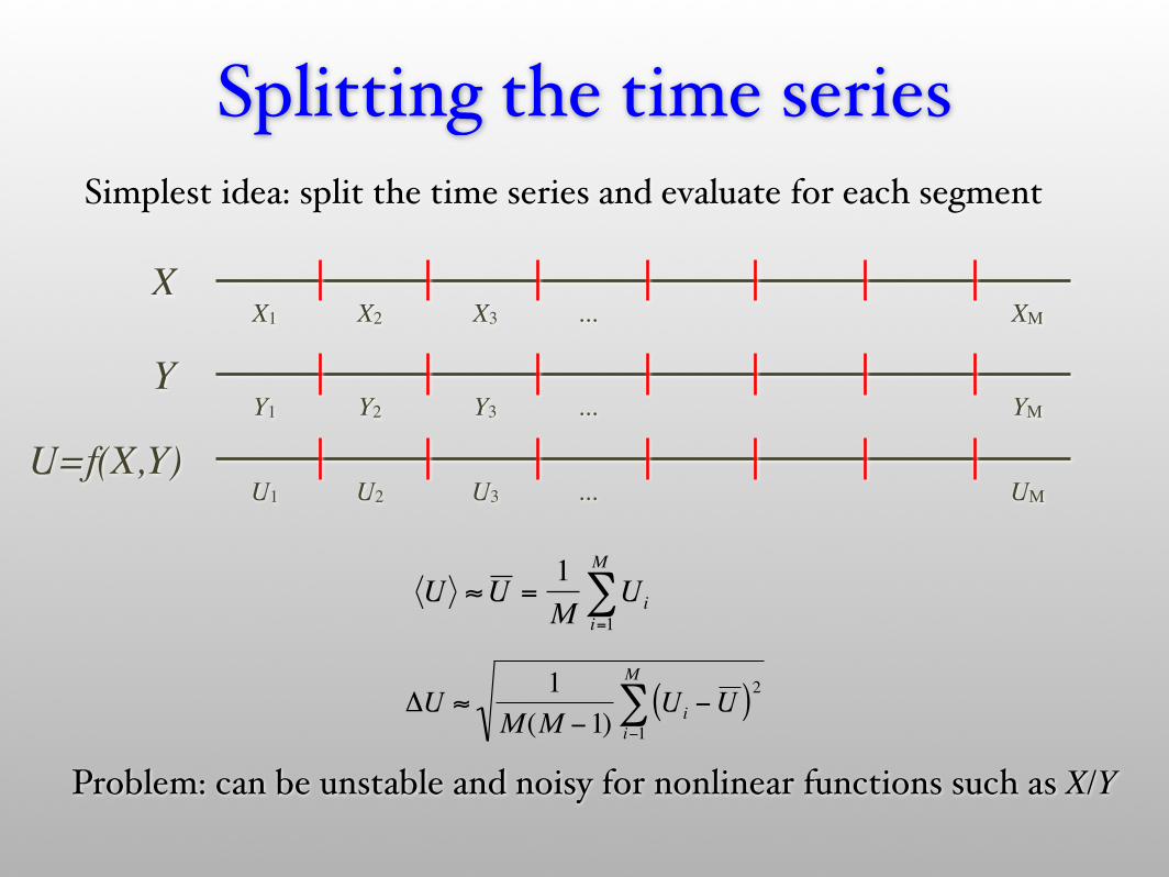
Splitting the time seriesSimplest idea: split the time series and evaluate for each segment
X
YX1 X2 X3 ... XM
Y1 Y2 Y3 ... YM
U=f(X,Y)U1 U2 U3 ... UM
Problem: can be unstable and noisy for nonlinear functions such as X/Y€
U ≈U =1M
Uii=1
M
∑
€
ΔU ≈1
M(M −1)Ui −U ( )2
i−1
M
∑
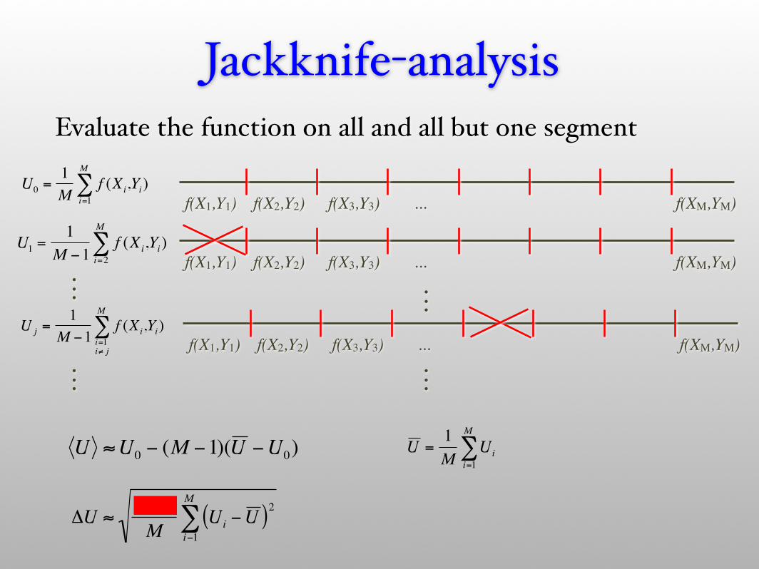
Jackknife-analysisEvaluate the function on all and all but one segment
Jackknife-analysisEvaluate the function on all and all but one segment
f(X1,Y1) f(X2,Y2) f(X3,Y3) ... f(XM,YM)
€
U0 =1M
f (Xi,Yi)i=1
M
∑
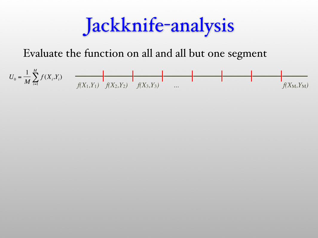
Jackknife-analysisEvaluate the function on all and all but one segment
f(X1,Y1) f(X2,Y2) f(X3,Y3) ... f(XM,YM)
€
U0 =1M
f (Xi,Yi)i=1
M
∑
f(X1,Y1) f(X2,Y2) f(X3,Y3) ... f(XM,YM)
€
U1 =1
M −1f (Xi,Yi)
i=2
M
∑

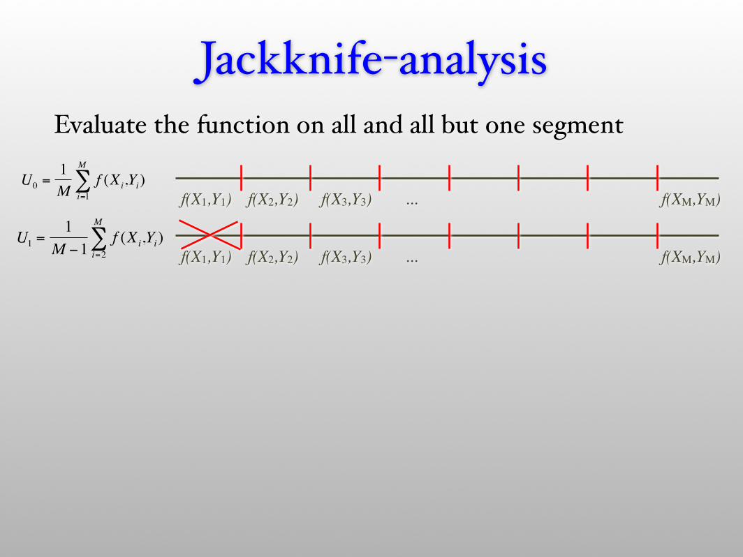
Jackknife-analysisEvaluate the function on all and all but one segment
f(X1,Y1) f(X2,Y2) f(X3,Y3) ... f(XM,YM)
€
U0 =1M
f (Xi,Yi)i=1
M
∑
f(X1,Y1) f(X2,Y2) f(X3,Y3) ... f(XM,YM)
€
U1 =1
M −1f (Xi,Yi)
i=2
M
∑
...f(X1,Y1) f(X2,Y2) f(X3,Y3) ... f(XM,YM)
€
U j =1
M −1f (Xi,Yi)
i=1i≠ j
M
∑
...
......
Jackknife-analysisEvaluate the function on all and all but one segment
f(X1,Y1) f(X2,Y2) f(X3,Y3) ... f(XM,YM)
€
U0 =1M
f (Xi,Yi)i=1
M
∑
f(X1,Y1) f(X2,Y2) f(X3,Y3) ... f(XM,YM)
€
U1 =1
M −1f (Xi,Yi)
i=2
M
∑
...f(X1,Y1) f(X2,Y2) f(X3,Y3) ... f(XM,YM)
€
U j =1
M −1f (Xi,Yi)
i=1i≠ j
M
∑
...
......
€
ΔU ≈M −1
MUi −U ( )2
i−1
M
∑€
U ≈U0 − (M −1)(U −U0)
€
U =1M
Uii=1
M
∑

ALPS.Alea library• The ALPS class library implements reliable error analysis
• Adding a measurement:
alps::RealObservable mag;…mag << new_value;
• Evaluating measurements
std::cout << mag.mean() << “ +/- “ << mag.error();std::cout “Autocorrelation time: “ << mag.tau();
• Correlated quantities?• Such as in Binder cumulant ratios
• ALPS library uses jackknife analysis to get correct errors
alps::RealObsEvaluator binder = mag4/(mag2*mag2);std::cout << binder.mean() << “ +/- “ << binder.error();
€
m4 m2 2
5. Critical slowing down, cluster updates and
Wang-Landau sampling

Autocorrelation effects
• The Metropolis algorithm creates a Markov chain
• successive configurations are correlated, leading to an increased statistical error
• Critical slowing down at second order phase transition
• Exponential tunneling problem at first order phase transition
c1→ c2 → ...→ ci → ci+1→ ...
ΔA = A − A( )2 =Var A
M(1+ 2τA )
τ ∝L2
τ ∝exp(Ld−1)
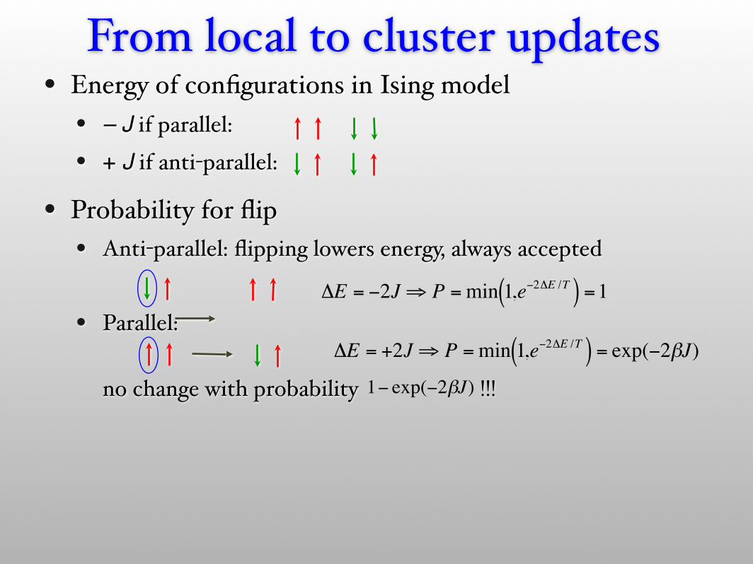
• Energy of configurations in Ising model• – J if parallel: • + J if anti-parallel:
• Probability for flip• Anti-parallel: flipping lowers energy, always accepted
• Parallel:
no change with probability !!!
From local to cluster updates
€
ΔE = −2J⇒ P =min 1,e−2ΔE /T( ) =1
€
ΔE = +2J⇒ P =min 1,e−2ΔE /T( ) = exp(−2βJ)
€
1− exp(−2βJ)
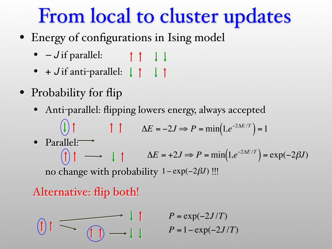
Alternative: flip both!
€
P = exp(−2J /T)P =1− exp(−2J /T)
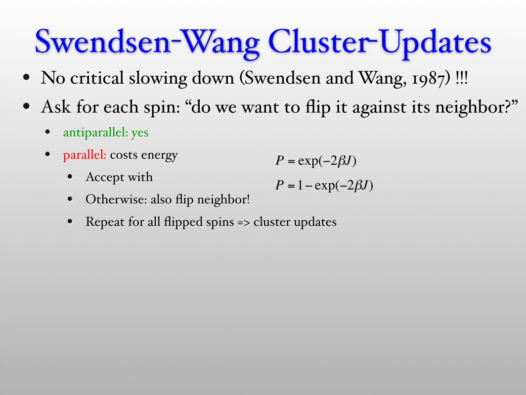
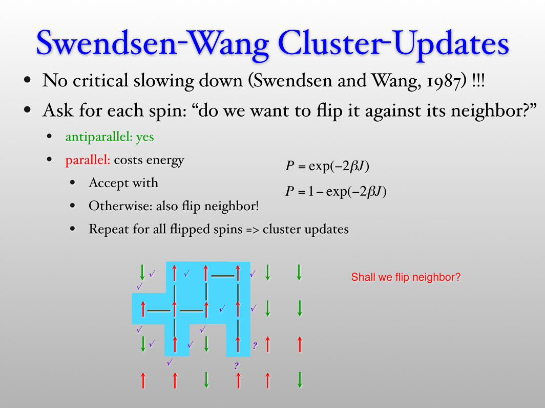
• No critical slowing down (Swendsen and Wang, 1987) !!! • Ask for each spin: “do we want to flip it against its neighbor?”
• antiparallel: yes
• parallel: costs energy
• Accept with
• Otherwise: also flip neighbor!
• Repeat for all flipped spins => cluster updates
Swendsen-Wang Cluster-Updates
€
P = exp(−2βJ)
€
P =1− exp(−2βJ)
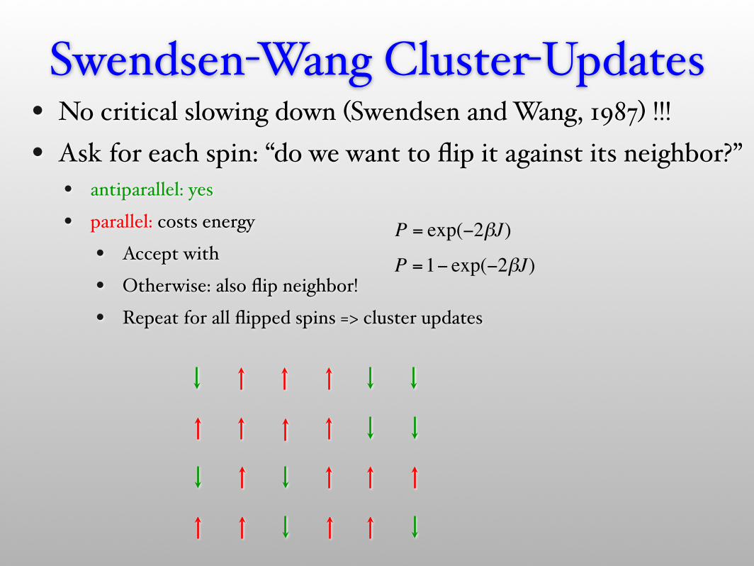

?
??
√
• No critical slowing down (Swendsen and Wang, 1987) !!! • Ask for each spin: “do we want to flip it against its neighbor?”
• antiparallel: yes
• parallel: costs energy
• Accept with
• Otherwise: also flip neighbor!
• Repeat for all flipped spins => cluster updates
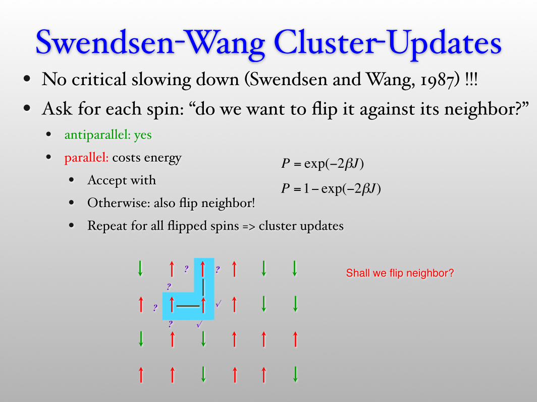
Swendsen-Wang Cluster-Updates
€
P = exp(−2βJ)
€
P =1− exp(−2βJ)
Shall we flip neighbor?
?
√?
√
?
??
• No critical slowing down (Swendsen and Wang, 1987) !!! • Ask for each spin: “do we want to flip it against its neighbor?”
• antiparallel: yes
• parallel: costs energy
• Accept with
• Otherwise: also flip neighbor!
• Repeat for all flipped spins => cluster updates
Swendsen-Wang Cluster-Updates
€
P = exp(−2βJ)
€
P =1− exp(−2βJ)
Shall we flip neighbor?
√
√
?
?
√
√
√
√ √
√√
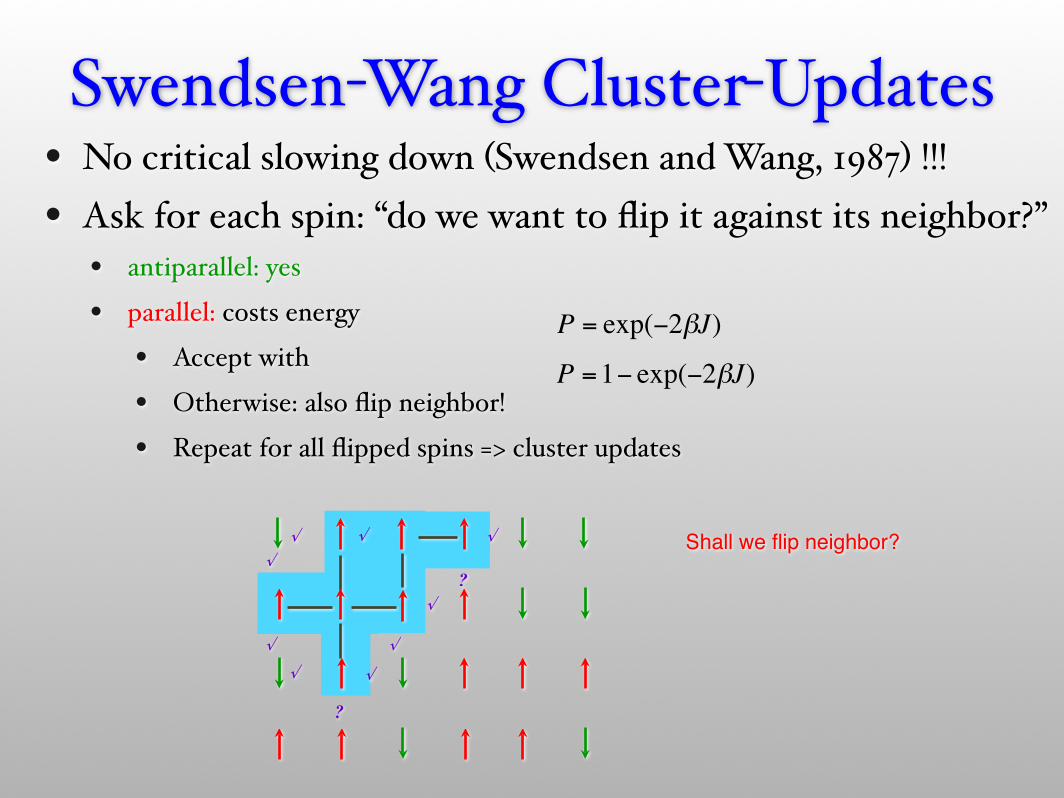
• No critical slowing down (Swendsen and Wang, 1987) !!! • Ask for each spin: “do we want to flip it against its neighbor?”
• antiparallel: yes
• parallel: costs energy
• Accept with
• Otherwise: also flip neighbor!
• Repeat for all flipped spins => cluster updates
Swendsen-Wang Cluster-Updates
€
P = exp(−2βJ)
€
P =1− exp(−2βJ)
Shall we flip neighbor?

• No critical slowing down (Swendsen and Wang, 1987) !!! • Ask for each spin: “do we want to flip it against its neighbor?”
• antiparallel: yes
• parallel: costs energy
• Accept with
• Otherwise: also flip neighbor!
• Repeat for all flipped spins => cluster updates
Swendsen-Wang Cluster-Updates
€
P = exp(−2βJ)
€
P =1− exp(−2βJ)
√
√ ?
√
√
√
√ √
√√
√
√
Shall we flip neighbor?
• No critical slowing down (Swendsen and Wang, 1987) !!! • Ask for each spin: “do we want to flip it against its neighbor?”
• antiparallel: yes
• parallel: costs energy
• Accept with
• Otherwise: also flip neighbor!
• Repeat for all flipped spins => cluster updates
Swendsen-Wang Cluster-Updates
€
P = exp(−2βJ)
€
P =1− exp(−2βJ)
√
√
√
√
√
√ √
√√
√
√
?
?
Shall we flip neighbor?

• No critical slowing down (Swendsen and Wang, 1987) !!! • Ask for each spin: “do we want to flip it against its neighbor?”
• antiparallel: yes
• parallel: costs energy
• Accept with
• Otherwise: also flip neighbor!
• Repeat for all flipped spins => cluster updates
Swendsen-Wang Cluster-Updates
€
P = exp(−2βJ)
€
P =1− exp(−2βJ)
√
√
√
√
√
√ √
√√
√
√
√
√
Shall we flip neighbor?

• No critical slowing down (Swendsen and Wang, 1987) !!! • Ask for each spin: “do we want to flip it against its neighbor?”
• antiparallel: yes
• parallel: costs energy
• Accept with
• Otherwise: also flip neighbor!
• Repeat for all flipped spins => cluster updates
Swendsen-Wang Cluster-Updates
€
P = exp(−2βJ)
€
P =1− exp(−2βJ)
√
√
√
√
√
√ √
√√
√
√
√
√ Done building clusterFlip all spins in cluster

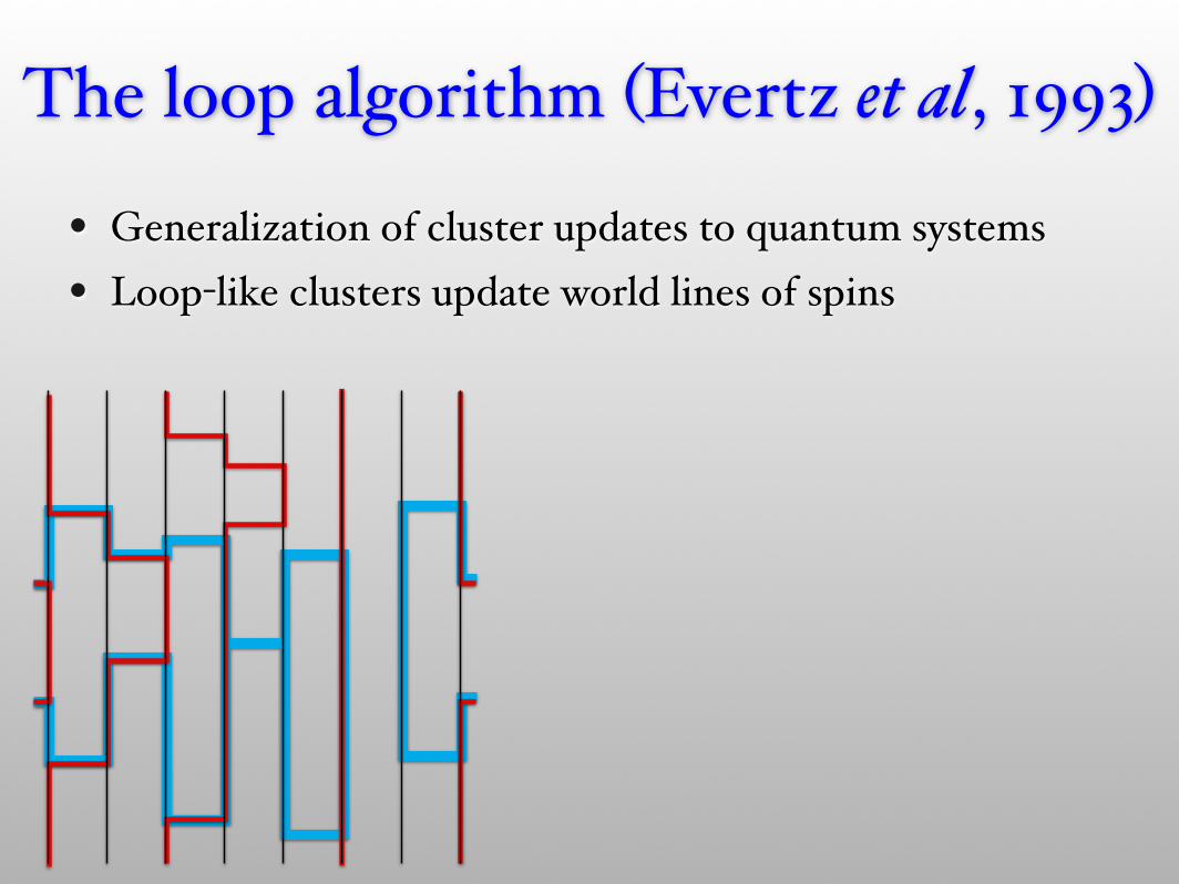
The loop algorithm (Evertz et al, 1993)
• Generalization of cluster updates to quantum systems• Loop-like clusters update world lines of spins
The loop algorithm (Evertz et al, 1993)
• Generalization of cluster updates to quantum systems• Loop-like clusters update world lines of spins
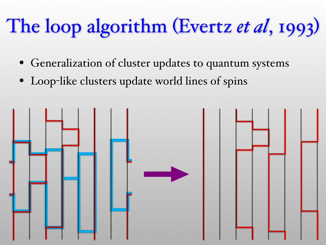
The loop algorithm (Evertz et al, 1993)
• Generalization of cluster updates to quantum systems• Loop-like clusters update world lines of spins

• Tunneling problem at a first order phase transition is solved by changing the ensemble to create a flat energy landscape• Multicanonical sampling (Berg and Neuhaus, Phys. Rev. Lett. 1992)• Wang-Landau sampling (Wang and Landau, Phys. Rev. Lett. 2001)• Quantum version (MT, Wessel and Alet, Phys. Rev. Lett. 2003)• Optimized ensembles (Trebst, Huse and MT, Phys. Rev. E 2004)
First order phase transitions
? ?liquid solid

2D ferromagnet
ln g(E)canonical weight
Canonical sampling
nw(E) = exp(!!E) g(E)
“critical energy”
nw(E)
2
~ 2N
energy
histogram
-1 0energy / 2N
ln( d
ensit
y of
stat
es )
Ec = E(Tc) ! 0.74E0

canonical weight
First-order phase transition
nw(E) = exp(!!E) g(E)
T=Tc
Exponentially suppressed tunneling out of metastable states.
10-state Potts model
ln g(E)
“critical energies”
energy
histogram
-1 0energy / 2N
ln( d
ensit
y of
stat
es )
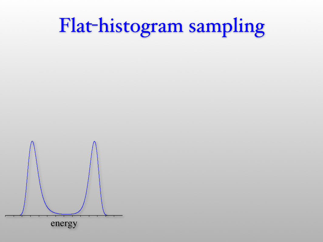
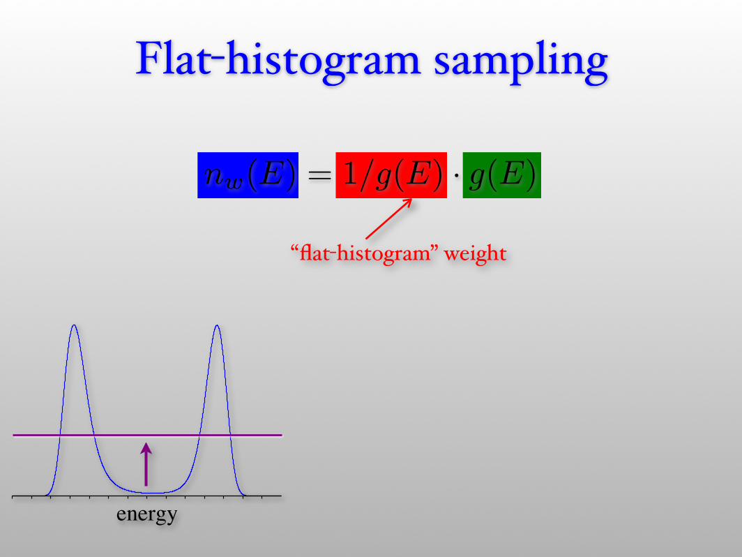
Flat-histogram sampling
energy

Flat-histogram sampling
energy
Flat-histogram sampling
“flat-histogram” weight
nw(E) = 1/g(E) · g(E)
energy

Flat-histogram sampling
“flat-histogram” weight
nw(E) = 1/g(E) · g(E)
How do we obtain the weights?
energy

Flat-histogram sampling
“flat-histogram” weight
nw(E) = 1/g(E) · g(E)
How do we obtain the weights?
energy
Flat-histogram MC algorithms Multicanonical recursions
Wang-Landau algorithm B. A. Berg and T. Neuhaus (1992)
F. Wang and D.P. Landau (2001)
Quantum versionM. Troyer, S. Wessel and F. Alet (2003)

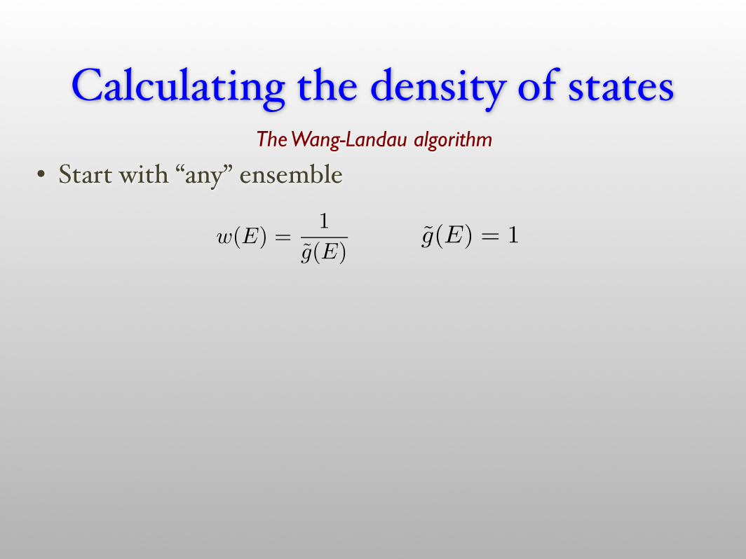
Calculating the density of statesThe Wang-Landau algorithm
Calculating the density of states
w(E) =1
g(E)
1
g(E) = 1
1
• Start with “any” ensembleThe Wang-Landau algorithm

estimateddensity of states
Calculating the density of states
w(E) =1
g(E)
1
g(E) = 1
1
• Start with “any” ensembleThe Wang-Landau algorithm
estimateddensity of states
Calculating the density of states
w(E) =1
g(E)
1
g(E) = 1
1
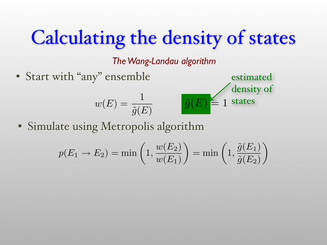
• Start with “any” ensemble
p(E1 ! E2) = min!
1,w(E2)w(E1)
"= min
!1,
g(E1)g(E2)
"
1
• Simulate using Metropolis algorithm
The Wang-Landau algorithm

estimateddensity of states
Calculating the density of states
w(E) =1
g(E)
1
g(E) = 1
1
• Start with “any” ensemble
p(E1 ! E2) = min!
1,w(E2)w(E1)
"= min
!1,
g(E1)g(E2)
"
1
• Simulate using Metropolis algorithm
g(E) = g(E) · f
1
• Iteratively improve ensemble during simulation
The Wang-Landau algorithm

modification factor
estimateddensity of states
Calculating the density of states
w(E) =1
g(E)
1
g(E) = 1
1
• Start with “any” ensemble
p(E1 ! E2) = min!
1,w(E2)w(E1)
"= min
!1,
g(E1)g(E2)
"
1
• Simulate using Metropolis algorithm
g(E) = g(E) · f
1
• Iteratively improve ensemble during simulation
• Reduce modification factor f when histogram is flat.
The Wang-Landau algorithm

Wang-Landau in actionMovie by Emanuel Gull (2004)

Wang-Landau in actionMovie by Emanuel Gull (2004)

6. The negative sign problem in quantum Monte Carlo

• Not as easy as classical Monte Carlo
• Calculating the eigenvalues Ec is equivalent to solving the problem
• Need to find a mapping of the quantum partition function to a classical problem
• “Negative sign” problem if some pc < 0
Quantum Monte Carlo
€
Z = e−Ec / kBTc∑
€
Z = Tre−βH ≡ pcc∑

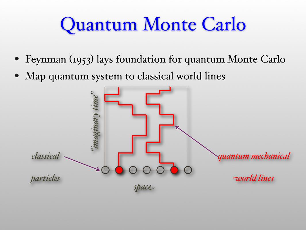
• Feynman (1953) lays foundation for quantum Monte Carlo• Map quantum system to classical world lines
Quantum Monte Carlo
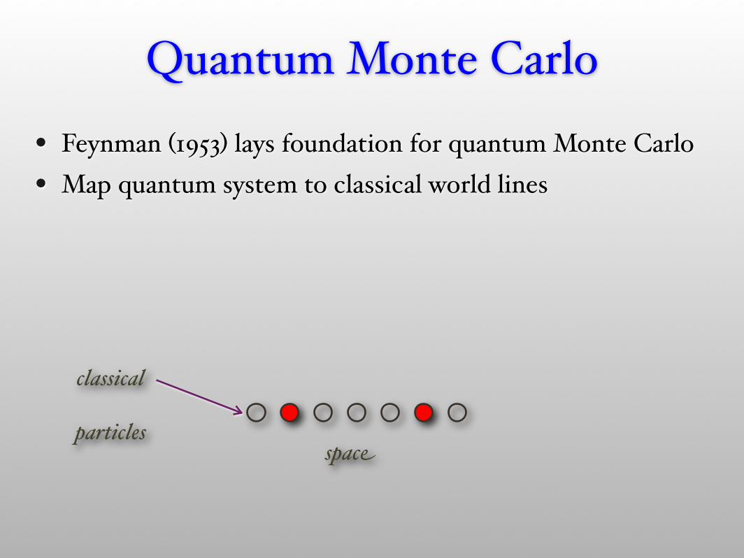
• Feynman (1953) lays foundation for quantum Monte Carlo• Map quantum system to classical world lines
Quantum Monte Carlo
space
classical
particles
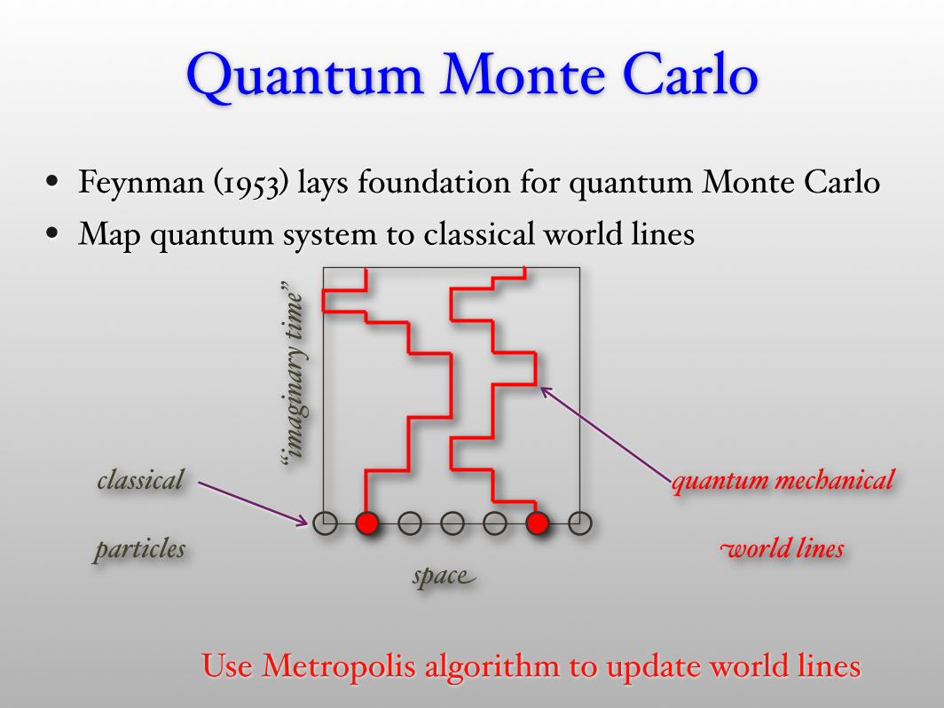
• Feynman (1953) lays foundation for quantum Monte Carlo• Map quantum system to classical world lines
Quantum Monte Carlo
“imag
inar
y tim
e”
quantum mechanical
world linesspace
classical
particles
• Feynman (1953) lays foundation for quantum Monte Carlo• Map quantum system to classical world lines
Quantum Monte Carlo
“imag
inar
y tim
e”
quantum mechanical
world linesspace
classical
particles
Use Metropolis algorithm to update world lines
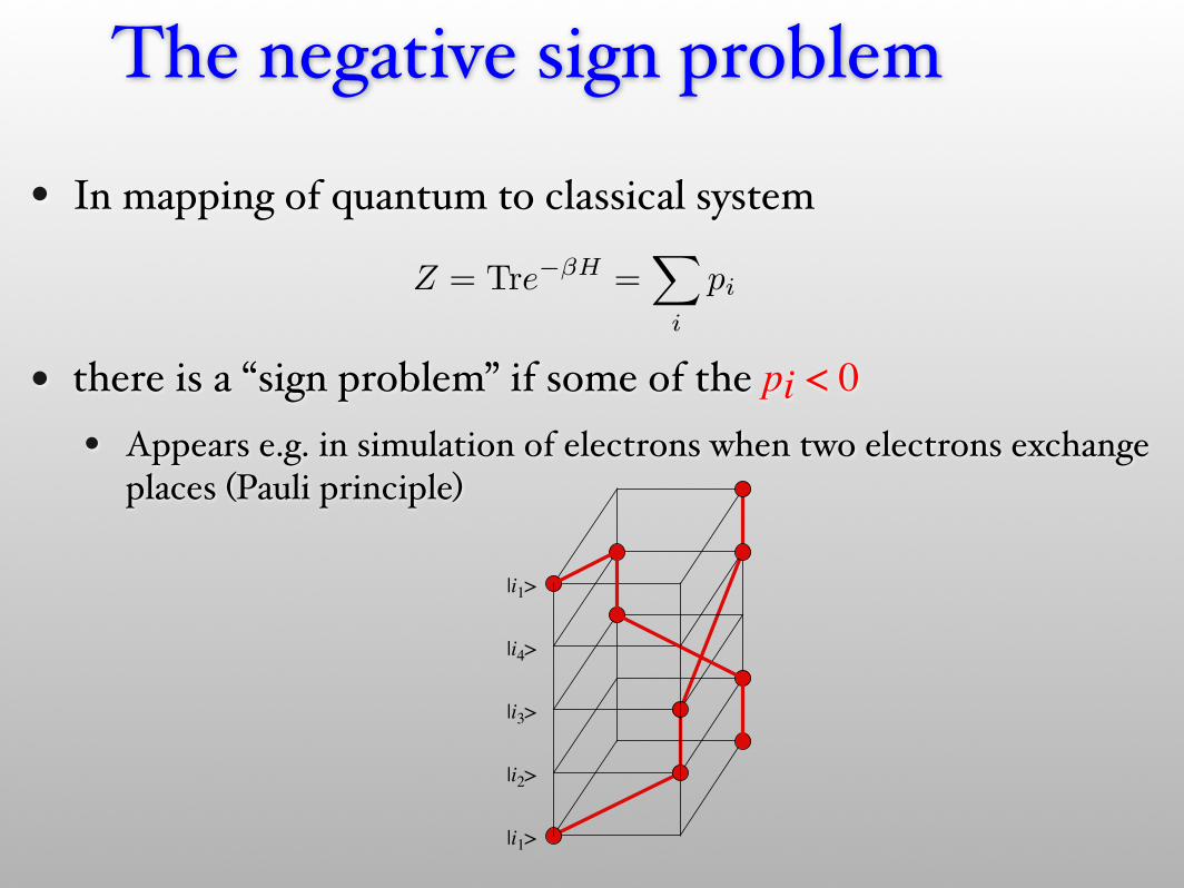
• In mapping of quantum to classical system
• there is a “sign problem” if some of the pi < 0• Appears e.g. in simulation of electrons when two electrons exchange
places (Pauli principle)
The negative sign problem
Z = Tre!!H=
!
i
pi
|i1>
|i2>
|i3>
|i4>
|i1>
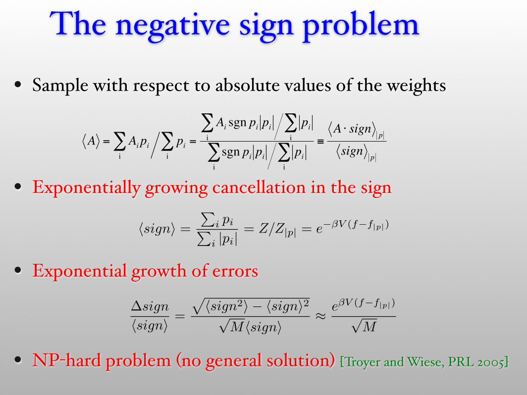
• Sample with respect to absolute values of the weights
• Exponentially growing cancellation in the sign
• Exponential growth of errors
• NP-hard problem (no general solution) [Troyer and Wiese, PRL 2005]
The negative sign problem
€
A = Aipii∑ pi
i∑ =
Ai sgn pi pii∑ pi
i∑
sgn pi pii∑ pi
i∑
≡A ⋅ sign p
sign p
!sign" =
!i pi!
i |pi|= Z/Z|p| = e!!V (f!f|p|)
!sign
!sign"=
!
!sign2" # !sign"2$M!sign"
%e!V (f!f|p|)
$M
The origin of the sign problem

The origin of the sign problem
• We sample with the wrong distribution by ignoring the sign!

The origin of the sign problem
• We sample with the wrong distribution by ignoring the sign!
• We simulate bosons and expect to learn about fermions?• will only work in insulators and superfluids

The origin of the sign problem
• We sample with the wrong distribution by ignoring the sign!
• We simulate bosons and expect to learn about fermions?• will only work in insulators and superfluids
• We simulate a ferromagnet and expect to learn something useful about a frustrated antiferromagnet?

The origin of the sign problem
• We sample with the wrong distribution by ignoring the sign!
• We simulate bosons and expect to learn about fermions?• will only work in insulators and superfluids
• We simulate a ferromagnet and expect to learn something useful about a frustrated antiferromagnet?
• We simulate a ferromagnet and expect to learn something about a spin glass?• This is the idea behind the proof of NP-hardness

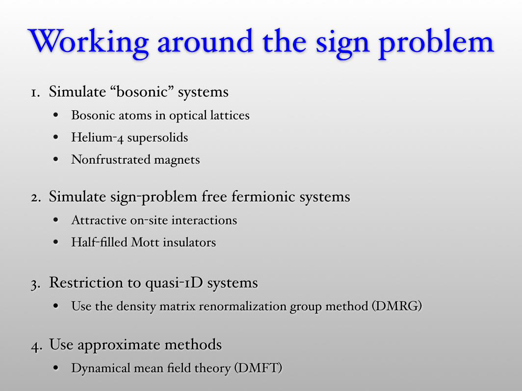
Working around the sign problem
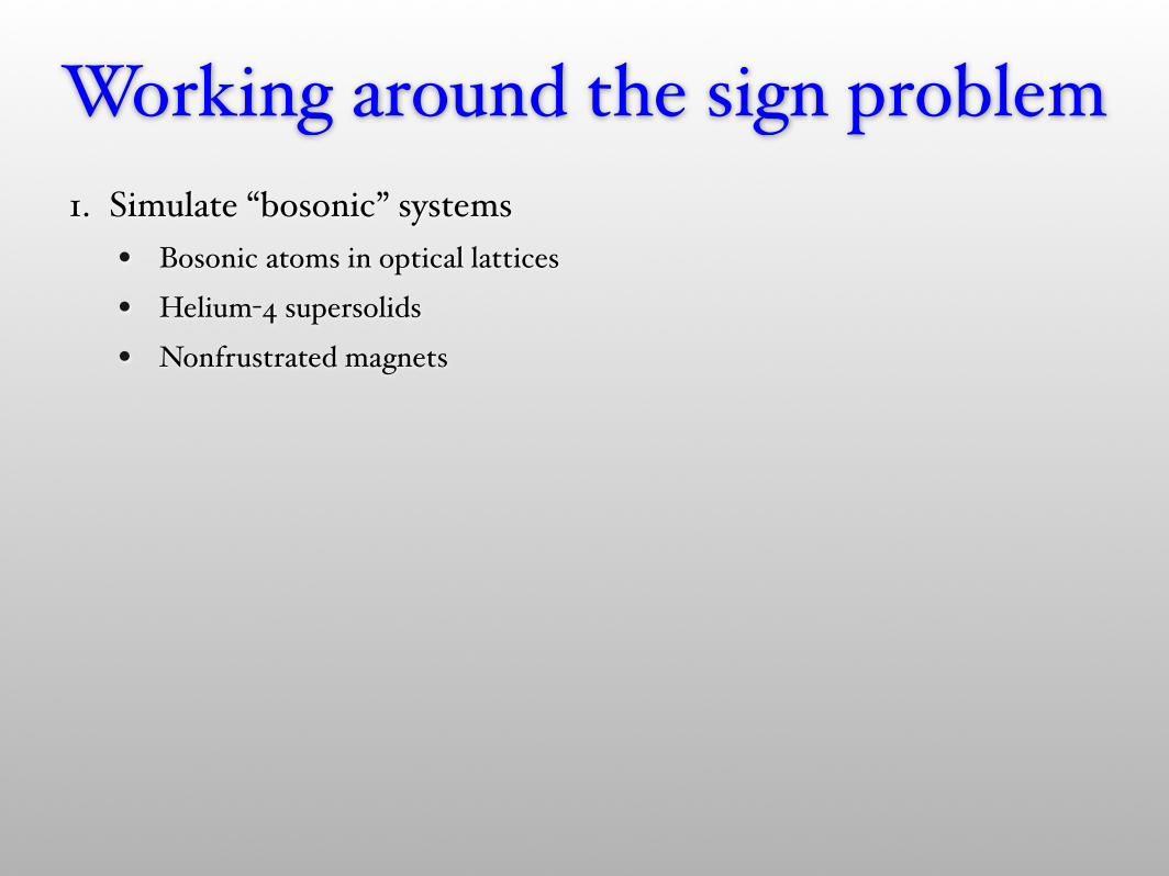
Working around the sign problem1. Simulate “bosonic” systems
• Bosonic atoms in optical lattices
• Helium-4 supersolids
• Nonfrustrated magnets

Working around the sign problem1. Simulate “bosonic” systems
• Bosonic atoms in optical lattices
• Helium-4 supersolids
• Nonfrustrated magnets
2. Simulate sign-problem free fermionic systems• Attractive on-site interactions
• Half-filled Mott insulators

Working around the sign problem1. Simulate “bosonic” systems
• Bosonic atoms in optical lattices
• Helium-4 supersolids
• Nonfrustrated magnets
2. Simulate sign-problem free fermionic systems• Attractive on-site interactions
• Half-filled Mott insulators
3. Restriction to quasi-1D systems• Use the density matrix renormalization group method (DMRG)
4. Use approximate methods• Dynamical mean field theory (DMFT)

7. Diverging Length Scalesand Finite Size Scaling

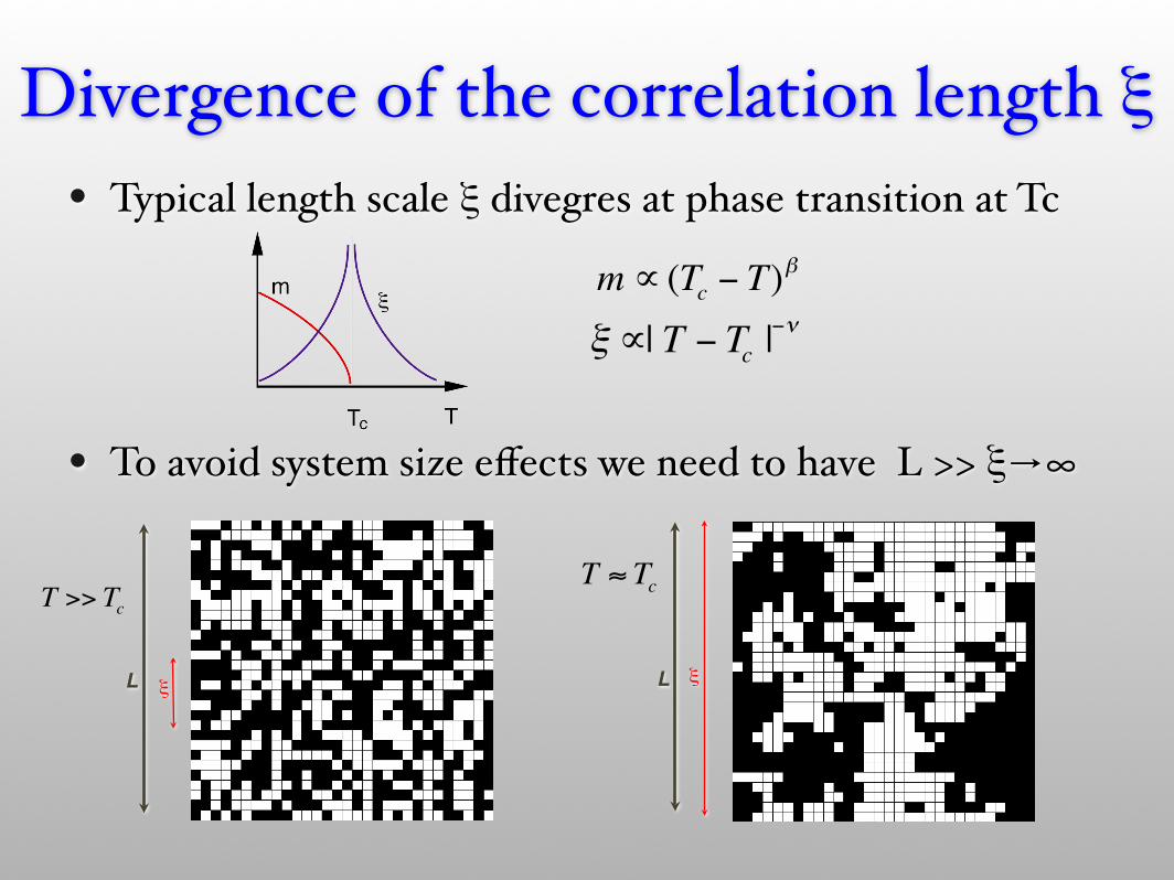
Divergence of the correlation length ξ• Typical length scale ξ divegres at phase transition at Tc
• To avoid system size effects we need to have L >> ξ→∞
m ∝ (Tc − T)β
ξ ∝| T − Tc |−ν
Divergence of the correlation length ξ• Typical length scale ξ divegres at phase transition at Tc
• To avoid system size effects we need to have L >> ξ→∞
m ∝ (Tc − T)β
ξ ∝| T − Tc |−ν
ξL
€
T >> Tc
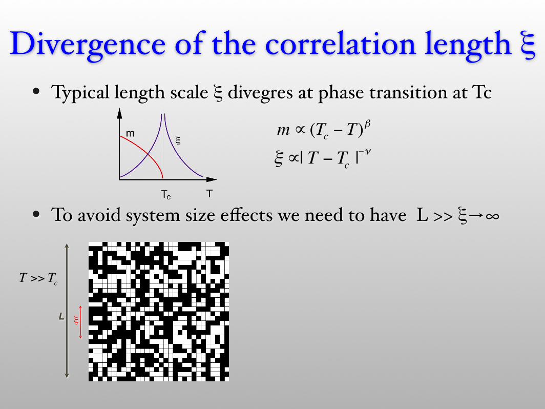
Divergence of the correlation length ξ• Typical length scale ξ divegres at phase transition at Tc
• To avoid system size effects we need to have L >> ξ→∞
m ∝ (Tc − T)β
ξ ∝| T − Tc |−ν
ξL
€
T >> Tc
ξL€
T ≈ Tc
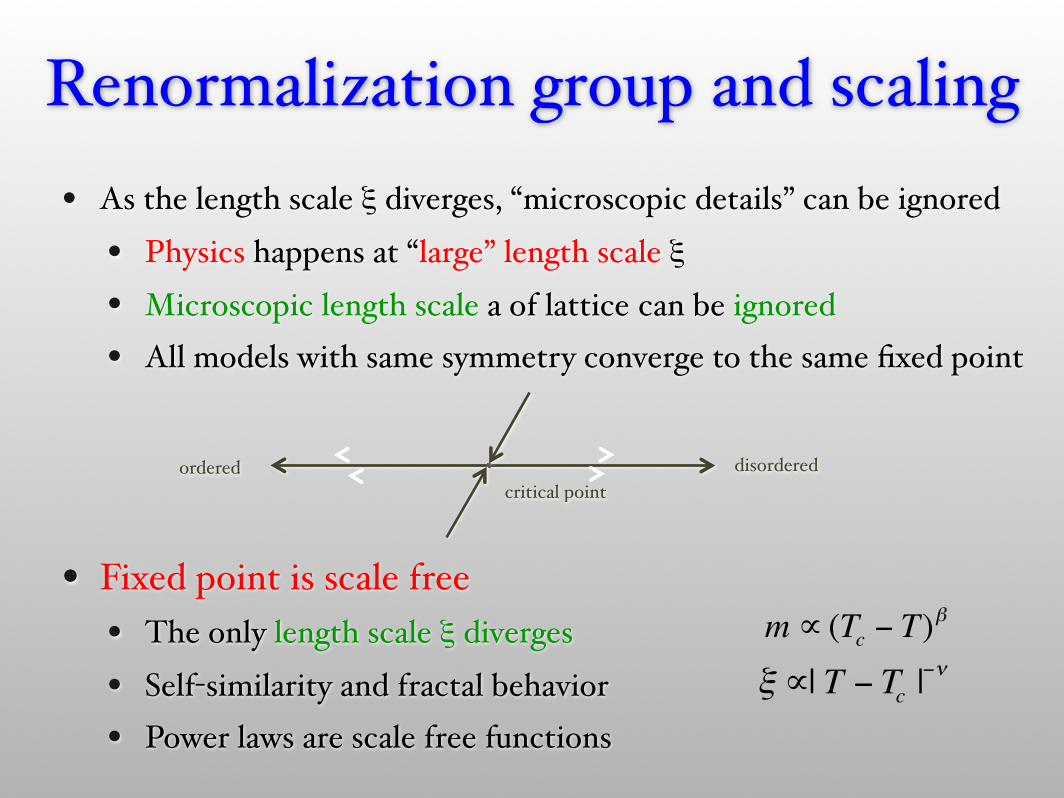
Renormalization group and scaling• As the length scale ξ diverges, “microscopic details” can be ignored
• Physics happens at “large” length scale ξ• Microscopic length scale a of lattice can be ignored• All models with same symmetry converge to the same fixed point
• Fixed point is scale free• The only length scale ξ diverges• Self-similarity and fractal behavior• Power laws are scale free functions
disorderedorderedcritical point
m ∝ (Tc − T)β
ξ ∝| T − Tc |−ν

• Infinite system
write M in terms of length scale ξ
• finite systems: L acts as cutoff to ξ
• We can obtain critical exponents β, ν from finite size effects
“Finite-size scaling”
ξL
€
€
ξ ∝ Tc −T( )−ν
€
M ∝ Tc −T( )β
€
⇒ M(T) = M(ξ)∝ξ−β /ν
€
M(T,L) = M(ξ,L) = M(ξ /L)∝ξ−β /ν L >> ξ
L−β /ν L << ξ

• Quantum phase transition in a 2D Heisenberg antiferromagnet• Susceptibility
• Structure factor of magnetization
• Scaling fits give z and η• Additional dynamical critical exponent z
is only difference from classical FSS
A quantum antiferromagnet
S(Q) = L2m ∝L2−z−η
χs ∝L2−η
1
10
100
1000
10 100L/a
Staggered suscpetibilityStaggered structurefactor
2-η = 1.985 ± 0.025
2-z-η = 0.967 ± 0.005
€
ξτ ∝ξz


