47
Statistics 514: Design and Analysis of Experiments Dr. Zhu Purdue University Spring 2005 Lecture 10: 2 k Factorial Design Montgomery: Chapter 6 March , 2005 Page 1

Statistics 514: Design and Analysis of ExperimentsDr. Zhu
Purdue UniversitySpring 2005
Lecture 10: 2k Factorial Design
Montgomery: Chapter 6
March , 2005Page 1
Statistics 514: Design and Analysis of ExperimentsDr. Zhu
Purdue UniversitySpring 2005
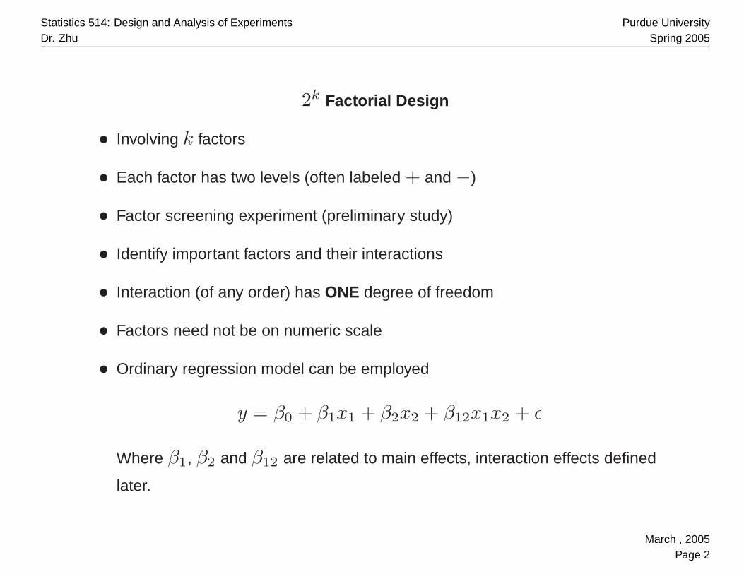
2k Factorial Design
• Involving k factors
• Each factor has two levels (often labeled + and −)
• Factor screening experiment (preliminary study)
• Identify important factors and their interactions
• Interaction (of any order) has ONE degree of freedom
• Factors need not be on numeric scale
• Ordinary regression model can be employed
y = β0 + β1x1 + β2x2 + β12x1x2 + ε
Where β1, β2 and β12 are related to main effects, interaction effects defined
later.
March , 2005Page 2

Statistics 514: Design and Analysis of ExperimentsDr. Zhu
Purdue UniversitySpring 2005
22 Factorial Design
Example:
factor replicate
A B treatment 1 2 3 mean
− − (1) 28 25 27 80/3
+ − a 36 32 32 100/3
− + b 18 19 23 60/3
+ + ab 31 30 29 90/3
• Let y(A+), y(A−), y(B+) and y(B−) be the level means of A and B.
• Let y(A−B−), y(A+B−), y(A−B+) and y(A+B+) be the treatment
means
March , 2005Page 3

Statistics 514: Design and Analysis of ExperimentsDr. Zhu
Purdue UniversitySpring 2005
Define main effects of A (denoted again by A ) as follows:
A = m.e.(A) = y(A+) − y(A−)
= 12 (y(A+B+) + y(A+B−)) − 1
2 (y(A−B+) + y(A−B−))= 1
2 (y(A+B+) + y(A+B−) − y(A−B+) − y(A−B−))= 1
2 (−y(A−B−) + y(A+B−) − y(A−B+) + y(A+B+))=8.33
• Let CA=(-1,1,-1,1), a contrast on treatment mean responses, then
m.e.(A)= 12 CA
• Notice that
A = m.e.(A) = (y(A+) − y..) − (y(A−) − y..) = τ2 − τ1
Main effect is defined in a different way than Chapter 5. But they are
connected and equivalent.
March , 2005Page 4

Statistics 514: Design and Analysis of ExperimentsDr. Zhu
Purdue UniversitySpring 2005
• Similarly
B = m.e.(B) = y(B+) − y(B−)
= 12(−y(A−B−) − y(A+B−)) + y(A−B+) + y(A+B+) =-5.00
Let CB=(-1,-1,1,1), a contrast on treatment mean responses, then B=m.e.(B)= 12CB
• Define interaction between A and B
AB = Int(AB) =1
2(m.e.(A | B+) − m.e.(A | B−))
=1
2(y(A+ | B+) − y(A− | B+)) − 1
2(y(A+ | B−) − y(A− | B−))
= 12(y(A−B−) − y(A+B−) − y(A−B+) + y(A+B+)) =1.67
Let CAB = (1,−1,−1, 1), a contrast on treatment means, then
AB=Int(AB)= 12CAB
March , 2005Page 5

Statistics 514: Design and Analysis of ExperimentsDr. Zhu
Purdue UniversitySpring 2005
Effects and Contrasts
factor effect (contrast)
A B total mean I A B AB
− − 80 80/3 1 -1 -1 1
+ − 100 100/3 1 1 -1 -1
− + 60 60/3 1 -1 1 -1
+ + 90 90/3 1 1 1 1
• There is a one-to-one correspondence between effects and constrasts, and
constrasts can be directly used to estimate the effects.
• For a effect corresponding to contrast c = (c1, c2, . . . ) in 22 design
effect =12
∑i
ciyi
where i is an index for treatments and the summation is over all treatments.
March , 2005Page 6

Statistics 514: Design and Analysis of ExperimentsDr. Zhu
Purdue UniversitySpring 2005
Sum of Squares due to Effect
• Because effects are defined using contrasts, their sum of squares can also be
calculated through contrasts.
• Recall for contrast c = (c1, c2, . . . ), its sum of squares is
SSContrast =(∑
ciyi)2
∑c2i /n
So
SSA =(−y(A−B−) + y(A+B−) − y(A−B+) + y(A+B+))2
4/n= 208.33
SSB =(−y(A−B−) − y(A+B−) + y(A−B+) + y(A+B+))2
4/n= 75.00
SSAB =(y(A−B−) − y(A+B−) − y(A−B+) + y(A+B+))2
4/n= 8.33
March , 2005Page 7
Statistics 514: Design and Analysis of ExperimentsDr. Zhu
Purdue UniversitySpring 2005
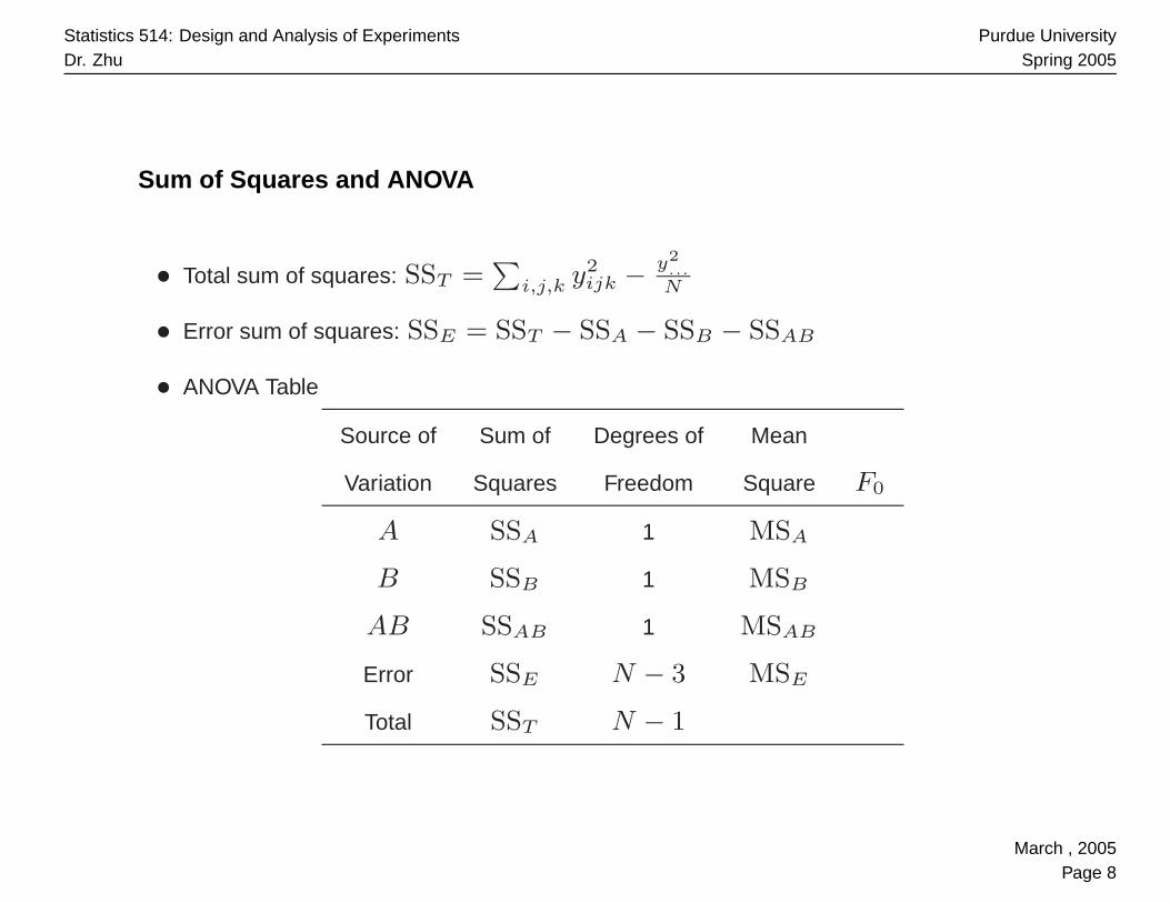
Sum of Squares and ANOVA
• Total sum of squares: SST =∑
i,j,k y2ijk − y2
...N
• Error sum of squares: SSE = SST − SSA − SSB − SSAB
• ANOVA Table
Source of Sum of Degrees of Mean
Variation Squares Freedom Square F0
A SSA 1 MSA
B SSB 1 MSB
AB SSAB 1 MSAB
Error SSE N − 3 MSE
Total SST N − 1
March , 2005Page 8
Statistics 514: Design and Analysis of ExperimentsDr. Zhu
Purdue UniversitySpring 2005
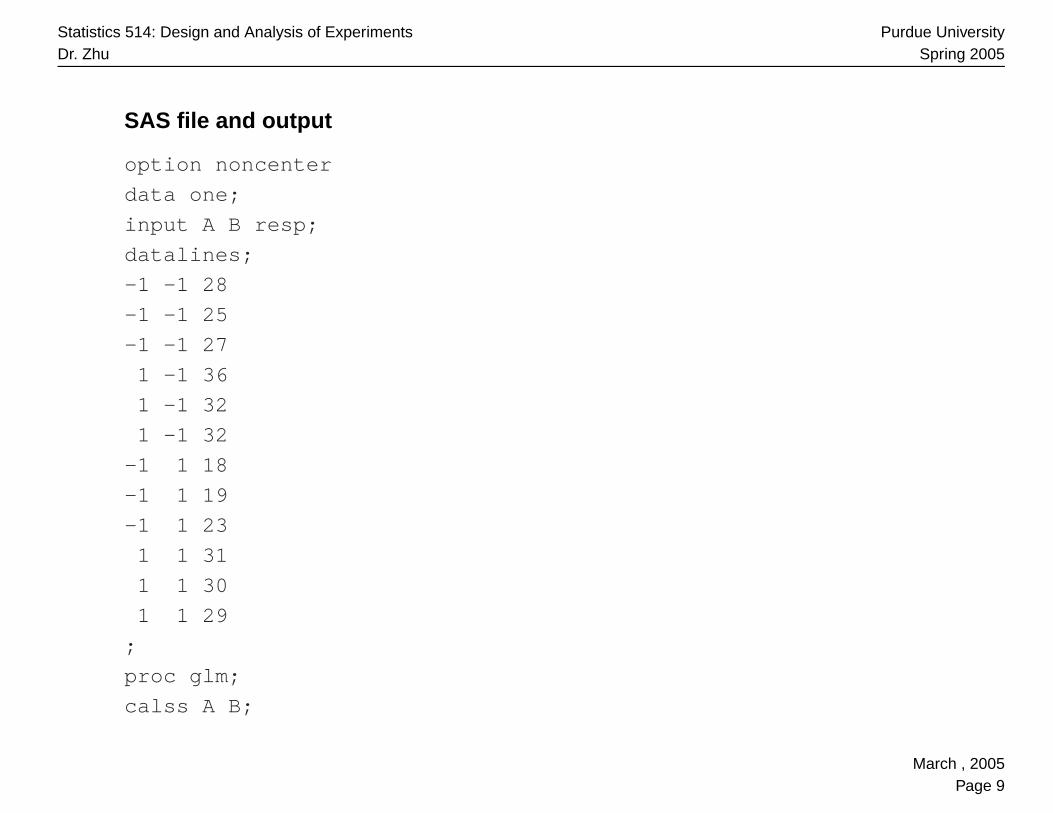
SAS file and output
option noncenter
data one;
input A B resp;
datalines;
-1 -1 28
-1 -1 25
-1 -1 27
1 -1 36
1 -1 32
1 -1 32
-1 1 18
-1 1 19
-1 1 23
1 1 31
1 1 30
1 1 29
;
proc glm;
calss A B;
March , 2005Page 9

Statistics 514: Design and Analysis of ExperimentsDr. Zhu
Purdue UniversitySpring 2005
model resp=A|B;
run;
---------------------------------------------------
Sum of
Source DF Squares Mean Square F Value Pr > F
Model 3 291.6666667 97.2222222 24.82 0.0002
Error 8 31.3333333 3.9166667
Cor Total 11 323.0000000
A 1 208.3333333 208.3333333 53.19 <.0001
B 1 75.0000000 75.0000000 19.15 0.0024
A*B 1 8.3333333 8.3333333 2.13 0.1828
March , 2005Page 10

Statistics 514: Design and Analysis of ExperimentsDr. Zhu
Purdue UniversitySpring 2005
Analyzing 22 Experiment Using Regresson Model
Because every effect in 22 design, or its sum of squares, have one degree of freedom, it
can be equivalently represented by a numerical variable, and regression analysis can be
directly used to analyze the data. The original factors are not necessasrily continuous.
Code the levels of factor A and B as follows
A x1 B x2
- -1 - -1
+ 1 + 1
Fit regression model
y = β0 + β1x1 + β2x2 + β12x1x2 + ε
The fitted model should be
y = y.. +A
2x1 +
B
2x2 +
AB
2x1x2
i.e. the estimated coefficients are half of the effects, respectively.
March , 2005Page 11

Statistics 514: Design and Analysis of ExperimentsDr. Zhu
Purdue UniversitySpring 2005
SAS Code and Output
option noncenter
data one;
input x1 x2 resp;
x1x2=x1*x2;
datalines;
-1 -1 28
-1 -1 25
-1 -1 27
........
1 1 31
1 1 30
1 1 29
;
proc reg;
model resp=x1 x2 x1x2;
run
March , 2005Page 12
Statistics 514: Design and Analysis of ExperimentsDr. Zhu
Purdue UniversitySpring 2005
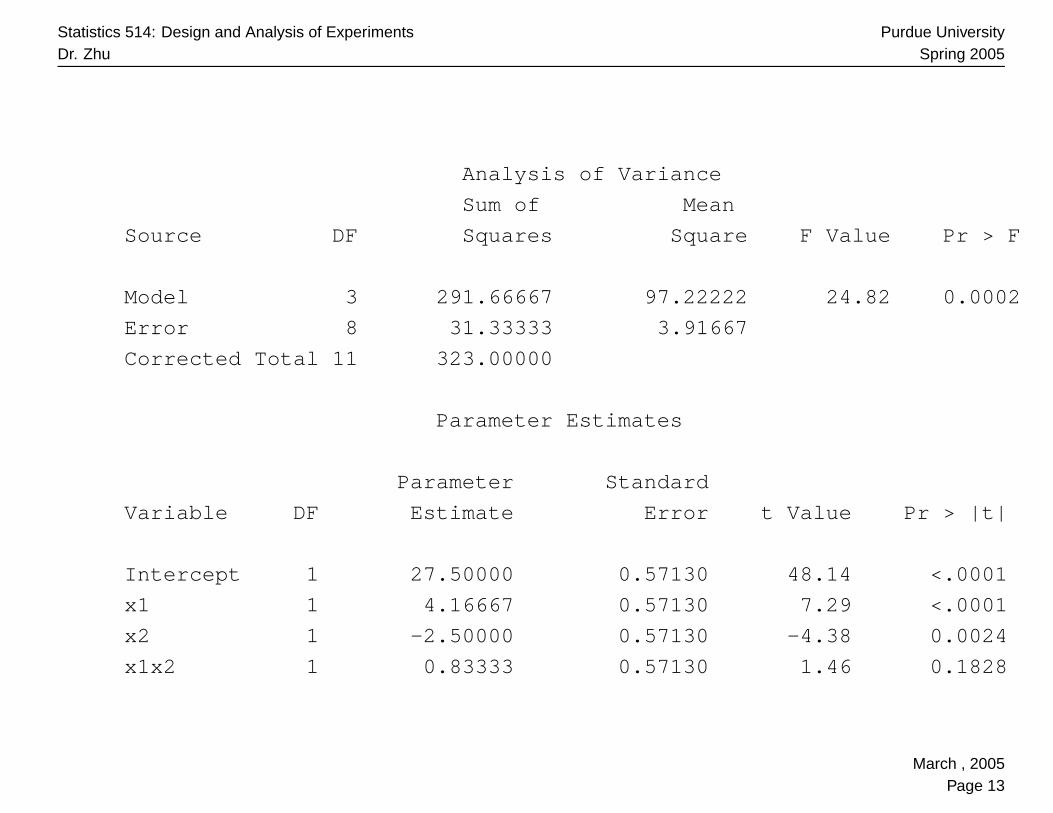
Analysis of Variance
Sum of Mean
Source DF Squares Square F Value Pr > F
Model 3 291.66667 97.22222 24.82 0.0002
Error 8 31.33333 3.91667
Corrected Total 11 323.00000
Parameter Estimates
Parameter Standard
Variable DF Estimate Error t Value Pr > |t|
Intercept 1 27.50000 0.57130 48.14 <.0001
x1 1 4.16667 0.57130 7.29 <.0001
x2 1 -2.50000 0.57130 -4.38 0.0024
x1x2 1 0.83333 0.57130 1.46 0.1828
March , 2005Page 13

Statistics 514: Design and Analysis of ExperimentsDr. Zhu
Purdue UniversitySpring 2005
23 Factorial Design
Bottling Experiment:
factor response
A B C treatment 1 2 total
− − − (1) -3 -1 -4
+ − − a 0 1 1
− + − b -1 0 -1
+ + − ab 2 3 5
− − + c -1 0 -1
+ − + ac 2 1 3
− + + bc 1 1 2
+ + + abc 6 5 11
March , 2005Page 14
Statistics 514: Design and Analysis of ExperimentsDr. Zhu
Purdue UniversitySpring 2005
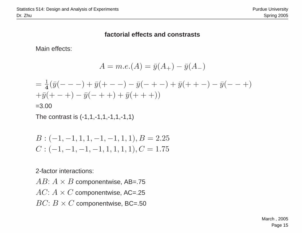
factorial effects and constrasts
Main effects:
A = m.e.(A) = y(A+) − y(A−)
= 14 (y(−−−) + y(+ −−) − y(− + −) + y(+ + −) − y(−− +)
+y(+ − +) − y(− + +) + y(+ + +))=3.00
The contrast is (-1,1,-1,1,-1,1,-1,1)
B : (−1,−1, 1, 1,−1,−1, 1, 1), B = 2.25C : (−1,−1,−1,−1, 1, 1, 1, 1), C = 1.75
2-factor interactions:
AB: A × B componentwise, AB=.75
AC : A × C componentwise, AC=.25
BC : B × C componentwise, BC=.50
March , 2005Page 15
Statistics 514: Design and Analysis of ExperimentsDr. Zhu
Purdue UniversitySpring 2005
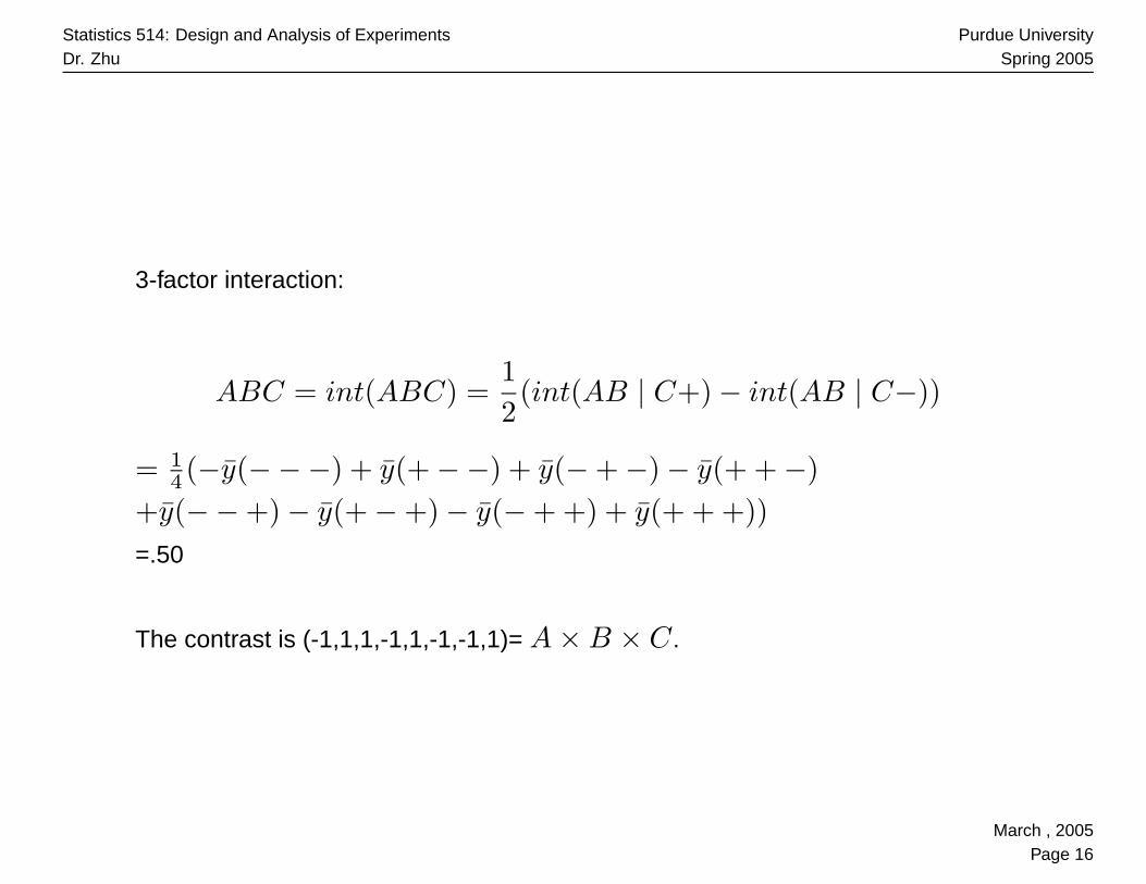
3-factor interaction:
ABC = int(ABC) =12(int(AB | C+) − int(AB | C−))
= 14 (−y(−−−) + y(+ −−) + y(− + −) − y(+ + −)
+y(−− +) − y(+ − +) − y(− + +) + y(+ + +))=.50
The contrast is (-1,1,1,-1,1,-1,-1,1)= A × B × C .
March , 2005Page 16
Statistics 514: Design and Analysis of ExperimentsDr. Zhu
Purdue UniversitySpring 2005
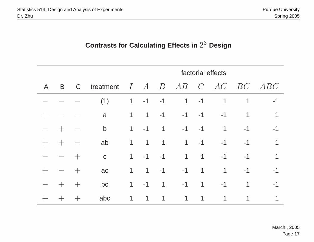
Contrasts for Calculating Effects in 23 Design
factorial effects
A B C treatment I A B AB C AC BC ABC
− − − (1) 1 -1 -1 1 -1 1 1 -1
+ − − a 1 1 -1 -1 -1 -1 1 1
− + − b 1 -1 1 -1 -1 1 -1 -1
+ + − ab 1 1 1 1 -1 -1 -1 1
− − + c 1 -1 -1 1 1 -1 -1 1
+ − + ac 1 1 -1 -1 1 1 -1 -1
− + + bc 1 -1 1 -1 1 -1 1 -1
+ + + abc 1 1 1 1 1 1 1 1
March , 2005Page 17

Statistics 514: Design and Analysis of ExperimentsDr. Zhu
Purdue UniversitySpring 2005
Estimates:
grand mean:
∑yi.
23
effect :∑
ciyi.
23−1
Contrast Sum of Squares:
SSeffect =(∑
ciyi.)2
23/n= 2n(effect)2
Variance of Estimate
Var(effect) =σ2
n23−2
t-test for effects (confidence interval approach)
effect ± tα/2,2k(n−1)S.E.(effect)
March , 2005Page 18

Statistics 514: Design and Analysis of ExperimentsDr. Zhu
Purdue UniversitySpring 2005
Regresson Model
Code the levels of factor A and B as follows
A x1 B x2 C x3
- -1 - -1 - -1
+ 1 + 1 + 1
Fit regression model
y = β0 + β1x1 + β2x2 + β3x3 + β12x1x2 + β13x1x3 + β23x2x3 + β123x1x2x3 + ε
The fitted model should be
y = y.. +A
2x1 +
B
2x2 +
C
2x3 +
AB
2x1x2 +
AC
2x1x3 +
BC
2x2x3 +
ABC
2x1x2x3
i.e. β = effect2
, and
Var(β) =σ2
n2k=
σ2
n23
March , 2005Page 19

Statistics 514: Design and Analysis of ExperimentsDr. Zhu
Purdue UniversitySpring 2005
SAS Code: Bottling Experiment
data bottle;
input A B C devi;
datalines;
-1 -1 -1 -3
-1 -1 -1 -1
1 -1 -1 0
1 -1 -1 1
-1 1 -1 -1
-1 1 -1 0
1 1 -1 2
1 1 -1 3
-1 -1 1 -1
-1 -1 1 0
1 -1 1 2
1 -1 1 1
-1 1 1 1
-1 1 1 1
1 1 1 6
1 1 1 5
March , 2005Page 20
Statistics 514: Design and Analysis of ExperimentsDr. Zhu
Purdue UniversitySpring 2005
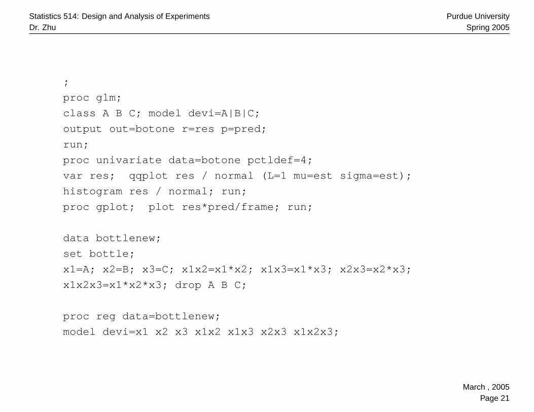
;
proc glm;
class A B C; model devi=A|B|C;
output out=botone r=res p=pred;
run;
proc univariate data=botone pctldef=4;
var res; qqplot res / normal (L=1 mu=est sigma=est);
histogram res / normal; run;
proc gplot; plot res*pred/frame; run;
data bottlenew;
set bottle;
x1=A; x2=B; x3=C; x1x2=x1*x2; x1x3=x1*x3; x2x3=x2*x3;
x1x2x3=x1*x2*x3; drop A B C;
proc reg data=bottlenew;
model devi=x1 x2 x3 x1x2 x1x3 x2x3 x1x2x3;
March , 2005Page 21
Statistics 514: Design and Analysis of ExperimentsDr. Zhu
Purdue UniversitySpring 2005
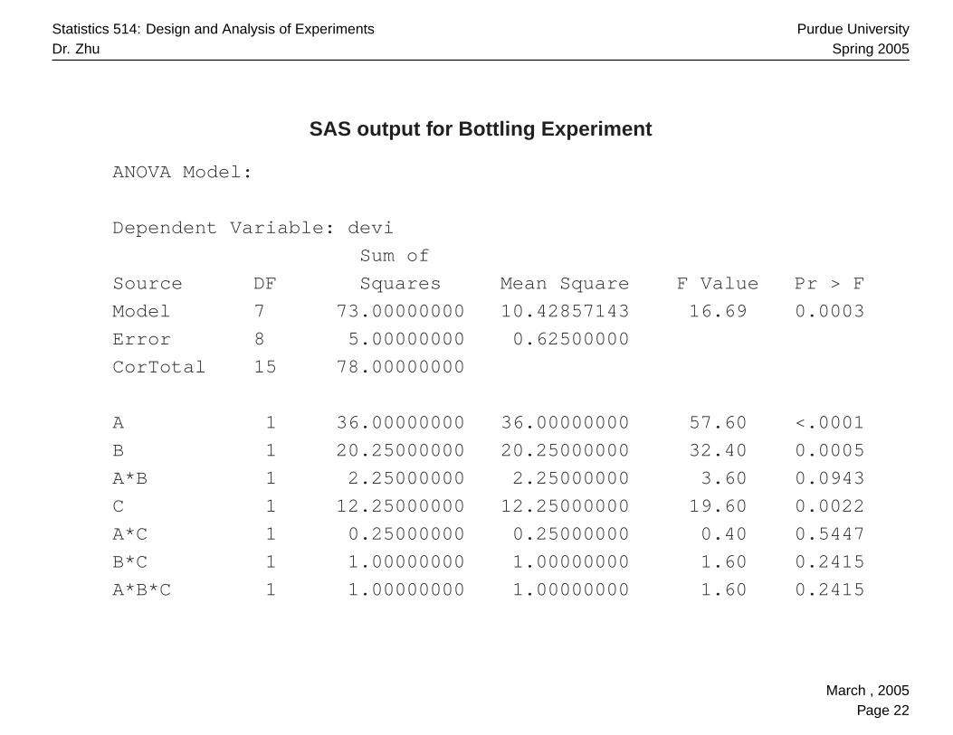
SAS output for Bottling Experiment
ANOVA Model:
Dependent Variable: devi
Sum of
Source DF Squares Mean Square F Value Pr > F
Model 7 73.00000000 10.42857143 16.69 0.0003
Error 8 5.00000000 0.62500000
CorTotal 15 78.00000000
A 1 36.00000000 36.00000000 57.60 <.0001
B 1 20.25000000 20.25000000 32.40 0.0005
A*B 1 2.25000000 2.25000000 3.60 0.0943
C 1 12.25000000 12.25000000 19.60 0.0022
A*C 1 0.25000000 0.25000000 0.40 0.5447
B*C 1 1.00000000 1.00000000 1.60 0.2415
A*B*C 1 1.00000000 1.00000000 1.60 0.2415
March , 2005Page 22

Statistics 514: Design and Analysis of ExperimentsDr. Zhu
Purdue UniversitySpring 2005
Regression Model:
Parameter Standard
Variable DF Estimate Error t Value Pr > |t|
Intercept 1 1.00000 0.19764 5.06 0.0010
x1 1 1.50000 0.19764 7.59 <.0001
x2 1 1.12500 0.19764 5.69 0.0005
x3 1 0.87500 0.19764 4.43 0.0022
x1x2 1 0.37500 0.19764 1.90 0.0943
x1x3 1 0.12500 0.19764 0.63 0.5447
x2x3 1 0.25000 0.19764 1.26 0.2415
x1x2x3 1 0.25000 0.19764 1.26 0.2415
March , 2005Page 23
Statistics 514: Design and Analysis of ExperimentsDr. Zhu
Purdue UniversitySpring 2005
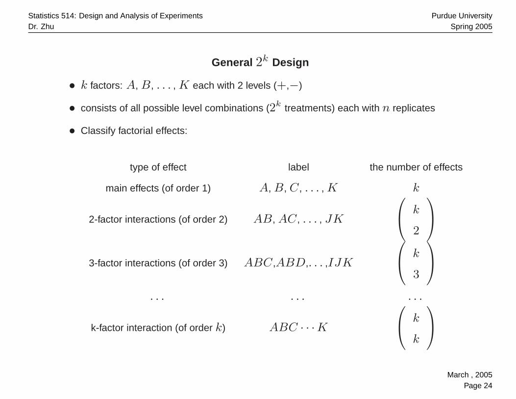
General 2k Design
• k factors: A, B, . . . , K each with 2 levels (+,−)
• consists of all possible level combinations (2k treatments) each with n replicates
• Classify factorial effects:
type of effect label the number of effects
main effects (of order 1) A, B, C , . . . , K k
2-factor interactions (of order 2) AB, AC , . . . , JK
k
2
3-factor interactions (of order 3) ABC ,ABD,. . . ,IJK
k
3
. . . . . . . . .
k-factor interaction (of order k) ABC · · ·K k
k
March , 2005Page 24
Statistics 514: Design and Analysis of ExperimentsDr. Zhu
Purdue UniversitySpring 2005
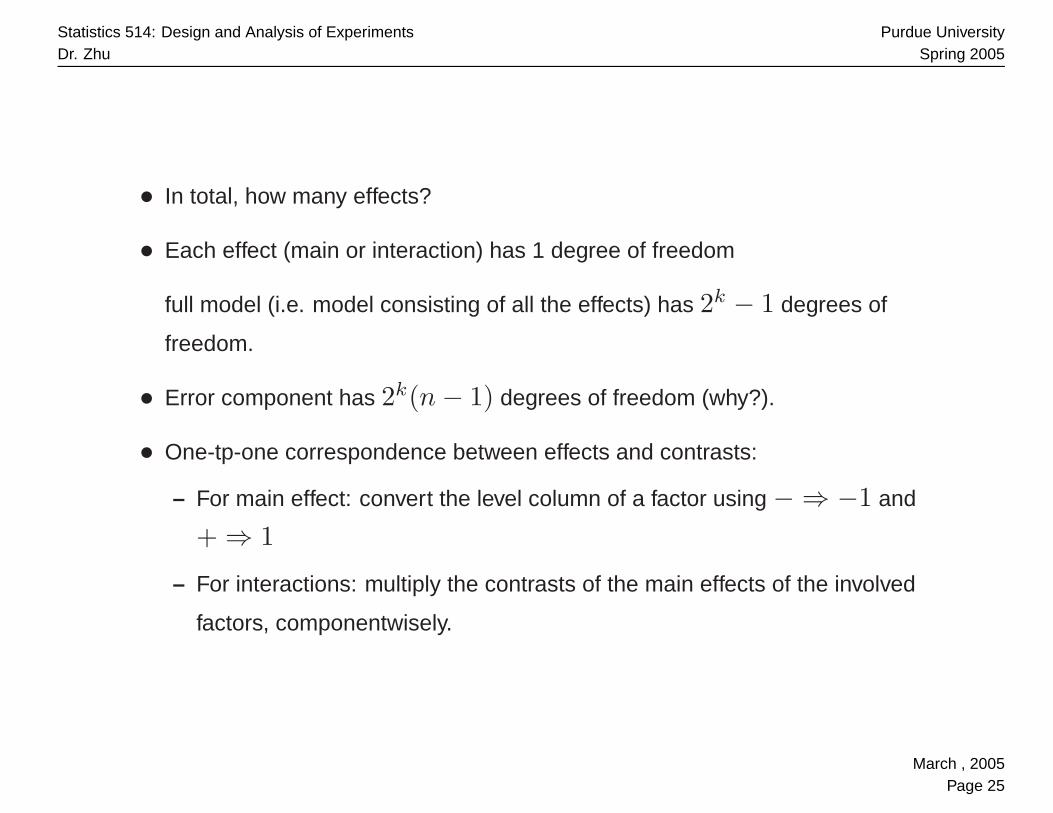
• In total, how many effects?
• Each effect (main or interaction) has 1 degree of freedom
full model (i.e. model consisting of all the effects) has 2k − 1 degrees of
freedom.
• Error component has 2k(n − 1) degrees of freedom (why?).
• One-tp-one correspondence between effects and contrasts:
– For main effect: convert the level column of a factor using − ⇒ −1 and
+ ⇒ 1
– For interactions: multiply the contrasts of the main effects of the involved
factors, componentwisely.
March , 2005Page 25
Statistics 514: Design and Analysis of ExperimentsDr. Zhu
Purdue UniversitySpring 2005
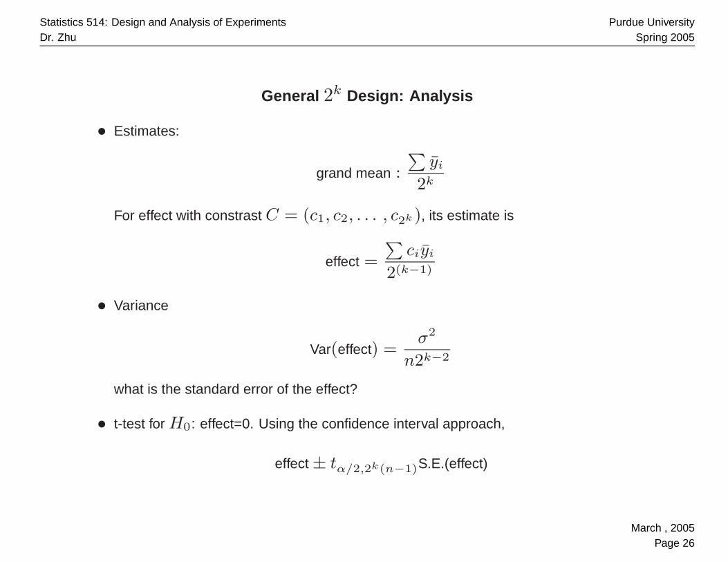
General 2k Design: Analysis
• Estimates:
grand mean :
∑yi
2k
For effect with constrast C = (c1, c2, . . . , c2k ), its estimate is
effect =
∑ciyi
2(k−1)
• Variance
Var(effect) =σ2
n2k−2
what is the standard error of the effect?
• t-test for H0: effect=0. Using the confidence interval approach,
effect ± tα/2,2k(n−1)S.E.(effect)
March , 2005Page 26

Statistics 514: Design and Analysis of ExperimentsDr. Zhu
Purdue UniversitySpring 2005
Using ANOVA model :
• Sum of Squares due to an effect, using its constrast,
SSeffect =
∑ciy
2i.
2k/n= n2k−2(effect)2
• SST and SSE can be calculated as before and a ANOVA table including SS due to
the effests and SSE can be constructed and the effects can be tested by F -tests.
Using regression :
• Introducing variables x1, . . . , xk for main effects, their products are used for
interactsions, the following regression model can be fitted
y = β0 + β1x1 + . . . + βkxk + . . . + β12···kx1x2 · · ·xk + ε
The coefficients are estimated by half of effects they represent, that is,
β =effect
2
March , 2005Page 27

Statistics 514: Design and Analysis of ExperimentsDr. Zhu
Purdue UniversitySpring 2005
Unreplicated 2k Design
Filtration Rate Experiment
March , 2005Page 28

Statistics 514: Design and Analysis of ExperimentsDr. Zhu
Purdue UniversitySpring 2005
factor
A B C D filtration
− − − − 45
+ − − − 71
− + − − 48
+ + − − 65
− − + − 68
+ − + − 60
− + + − 80
+ + + − 65
− − − + 43
+ − − + 100
− + − + 45
+ + − + 104
− − + + 75
+ − + + 86
− + + + 70
+ + + + 96
March , 2005Page 29
Statistics 514: Design and Analysis of ExperimentsDr. Zhu
Purdue UniversitySpring 2005
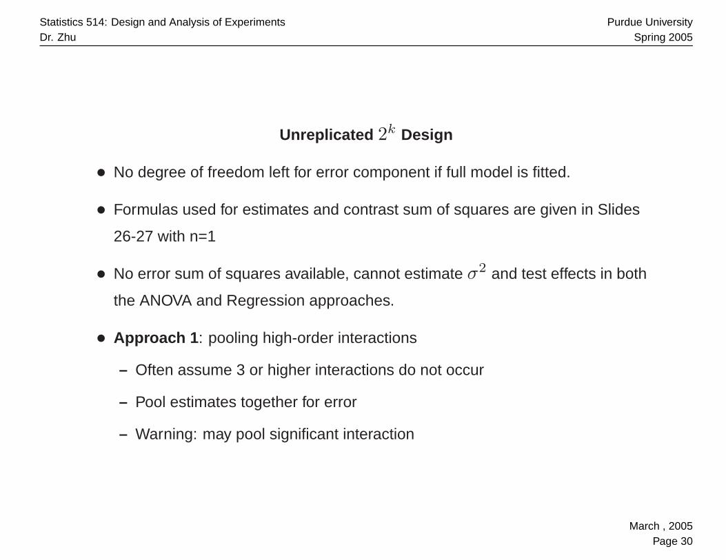
Unreplicated 2k Design
• No degree of freedom left for error component if full model is fitted.
• Formulas used for estimates and contrast sum of squares are given in Slides
26-27 with n=1
• No error sum of squares available, cannot estimate σ2 and test effects in both
the ANOVA and Regression approaches.
• Approach 1 : pooling high-order interactions
– Often assume 3 or higher interactions do not occur
– Pool estimates together for error
– Warning: may pool significant interaction
March , 2005Page 30
Statistics 514: Design and Analysis of ExperimentsDr. Zhu
Purdue UniversitySpring 2005
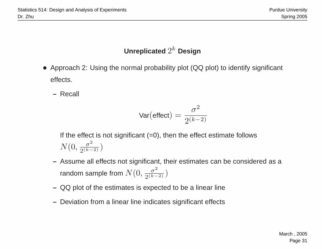
Unreplicated 2k Design
• Approach 2: Using the normal probability plot (QQ plot) to identify significant
effects.
– Recall
Var(effect) =σ2
2(k−2)
If the effect is not significant (=0), then the effect estimate follows
N(0, σ2
2(k−2) )
– Assume all effects not significant, their estimates can be considered as a
random sample from N(0, σ2
2(k−2) )
– QQ plot of the estimates is expected to be a linear line
– Deviation from a linear line indicates significant effects
March , 2005Page 31

Statistics 514: Design and Analysis of ExperimentsDr. Zhu
Purdue UniversitySpring 2005
Using SAS to generate QQ plot for effects
goption colors=(none);
data filter;
do D = -1 to 1 by 2;do C = -1 to 1 by 2;
do B = -1 to 1 by 2;do A = -1 to 1 by 2;
input y @@; output;
end; end; end; end;
datalines;
45 71 48 65 68 60 80 65 43 100 45 104 75 86 70 96
;
data inter; /* Define Interaction Terms */
set filter;
AB=A*B; AC=A*C; AD=A*D; BC=B*C; BD=B*D; CD=C*D; ABC=AB*C; ABD=AB*D;
ACD=AC*D; BCD=BC*D; ABCD=ABC*D;
proc glm data=inter; /* GLM Proc to Obtain Effects */
class A B C D AB AC AD BC BD CD ABC ABD ACD BCDABCD;
model y=A B C D AB AC AD BC BD CD ABC ABD ACD BCDABCD;
March , 2005Page 32
Statistics 514: Design and Analysis of ExperimentsDr. Zhu
Purdue UniversitySpring 2005
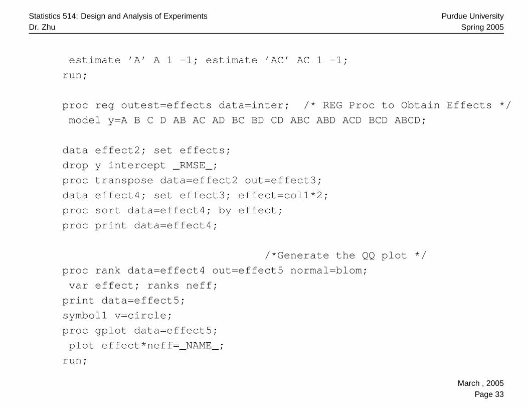
estimate ’A’ A 1 -1; estimate ’AC’ AC 1 -1;
run;
proc reg outest=effects data=inter; /* REG Proc to Obtain Effects */
model y=A B C D AB AC AD BC BD CD ABC ABD ACD BCDABCD;
data effect2; set effects;
drop y intercept _RMSE_;
proc transpose data=effect2 out=effect3;
data effect4; set effect3; effect=col1*2;
proc sort data=effect4; by effect;
proc print data=effect4;
/*Generate the QQ plot */
proc rank data=effect4 out=effect5 normal=blom;
var effect; ranks neff;
print data=effect5;
symbol1 v=circle;
proc gplot data=effect5;
plot effect*neff=_NAME_;
run;
March , 2005Page 33
Statistics 514: Design and Analysis of ExperimentsDr. Zhu
Purdue UniversitySpring 2005
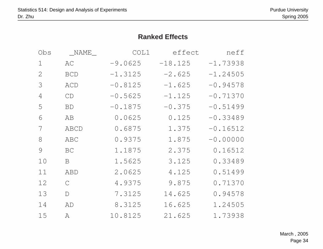
Ranked Effects
Obs _NAME_ COL1 effect neff
1 AC -9.0625 -18.125 -1.73938
2 BCD -1.3125 -2.625 -1.24505
3 ACD -0.8125 -1.625 -0.94578
4 CD -0.5625 -1.125 -0.71370
5 BD -0.1875 -0.375 -0.51499
6 AB 0.0625 0.125 -0.33489
7 ABCD 0.6875 1.375 -0.16512
8 ABC 0.9375 1.875 -0.00000
9 BC 1.1875 2.375 0.16512
10 B 1.5625 3.125 0.33489
11 ABD 2.0625 4.125 0.51499
12 C 4.9375 9.875 0.71370
13 D 7.3125 14.625 0.94578
14 AD 8.3125 16.625 1.24505
15 A 10.8125 21.625 1.73938
March , 2005Page 34
Statistics 514: Design and Analysis of ExperimentsDr. Zhu
Purdue UniversitySpring 2005
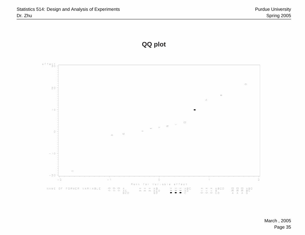
QQ plot
March , 2005Page 35

Statistics 514: Design and Analysis of ExperimentsDr. Zhu
Purdue UniversitySpring 2005
Filtration Experiment Analysis
Fit a linear line based on small effects, identify the effects which are potentially
significant, then use ANOVA or regression fit a sub-model with those effects.
1. Potentially significant effects: A, AD, C, D, AC .
2. Use main effect plot and interaction plot
3. ANOVA model involving only A, C , D and their interactions (projecting the
original unreplicated 24 experiment onto a replicated 23 experiement)
4. regression model only involving A, C , D, AC and AD.
5. Diagnostics using residuals.
March , 2005Page 36
Statistics 514: Design and Analysis of ExperimentsDr. Zhu
Purdue UniversitySpring 2005
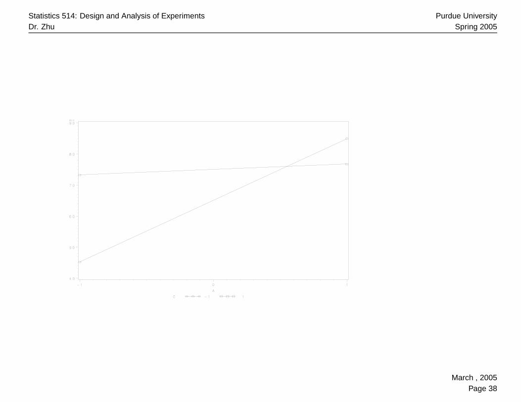
Interaction Plots for AC and AD
* data step is the same.
proc sort; by A C;
proc means noprint;
var y; by A C;
output out=ymeanac mean=mn;
symbol1 v=circle i=join; symbol2 v=square i=join;
proc gplot data=ymeanac; plot mn*A=C;
run;
* similar code for AD interaction plot
March , 2005Page 37
Statistics 514: Design and Analysis of ExperimentsDr. Zhu
Purdue UniversitySpring 2005
March , 2005Page 38

Statistics 514: Design and Analysis of ExperimentsDr. Zhu
Purdue UniversitySpring 2005
March , 2005Page 39
Statistics 514: Design and Analysis of ExperimentsDr. Zhu
Purdue UniversitySpring 2005
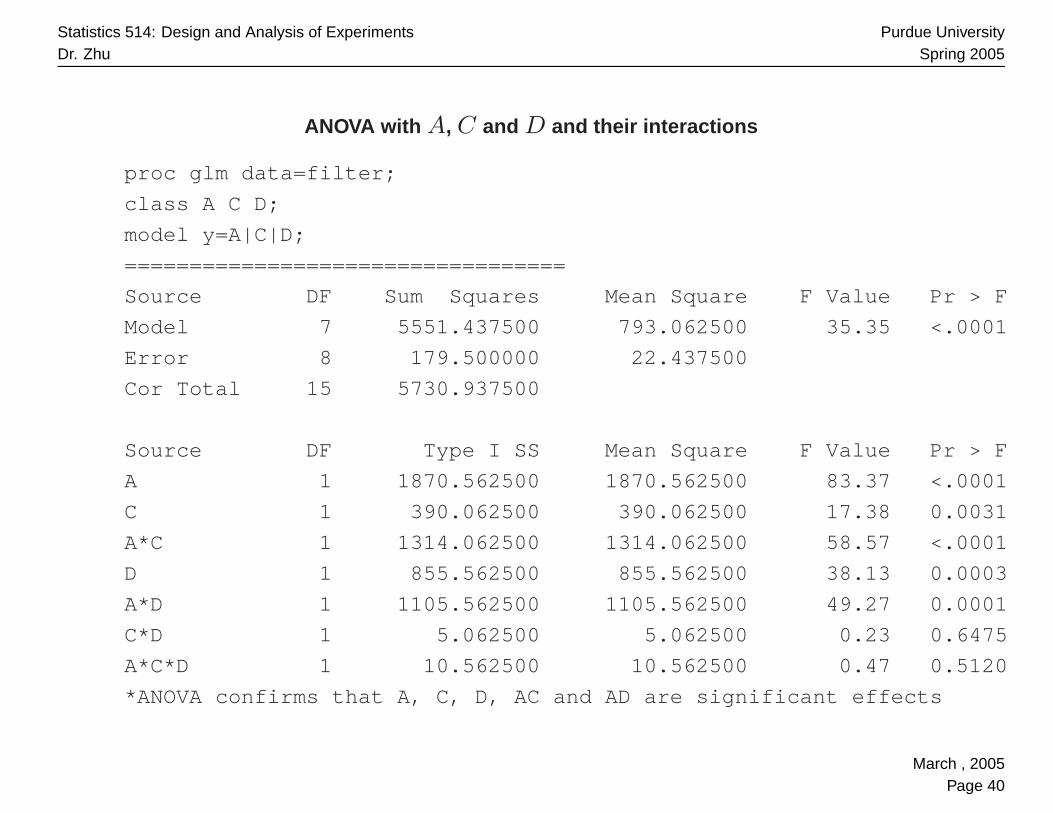
ANOVA with A, C and D and their interactions
proc glm data=filter;
class A C D;
model y=A|C|D;
==================================
Source DF Sum Squares Mean Square F Value Pr > F
Model 7 5551.437500 793.062500 35.35 <.0001
Error 8 179.500000 22.437500
Cor Total 15 5730.937500
Source DF Type I SS Mean Square F Value Pr > F
A 1 1870.562500 1870.562500 83.37 <.0001
C 1 390.062500 390.062500 17.38 0.0031
A*C 1 1314.062500 1314.062500 58.57 <.0001
D 1 855.562500 855.562500 38.13 0.0003
A*D 1 1105.562500 1105.562500 49.27 0.0001
C*D 1 5.062500 5.062500 0.23 0.6475
A*C*D 1 10.562500 10.562500 0.47 0.5120
*ANOVA confirms that A, C, D, AC and AD are significant effects
March , 2005Page 40

Statistics 514: Design and Analysis of ExperimentsDr. Zhu
Purdue UniversitySpring 2005
Regression Model
* the same date step
data inter; set filter; AC=A*C; AD=A*D;
proc reg data=inter; model y=A C D AC AD;
output out=outres r=res p=pred;
proc gplot data=outres; plot res*pred; run;
===========================
Dependent Variable: y
Analysis of Variance
Sum of Mean
Source DF Squares Square F Value Pr > F
Model 5 5535.81250 1107.16250 56.74 <.0001
Error 10 195.12500 19.51250
Corrected Total 15 5730.93750
Root MSE 4.41730 R-Square 0.9660
March , 2005Page 41

Statistics 514: Design and Analysis of ExperimentsDr. Zhu
Purdue UniversitySpring 2005
Dependent Mean 70.06250 Adj R-Sq 0.9489
Coeff Var 6.30479
Parameter Estimates
Parameter Standard
Variable DF Estimate Error t Value Pr > |t|
Intercept 1 70.06250 1.10432 63.44 <.0001
A 1 10.81250 1.10432 9.79 <.0001
C 1 4.93750 1.10432 4.47 0.0012
D 1 7.31250 1.10432 6.62 <.0001
AC 1 -9.06250 1.10432 -8.21 <.0001
AD 1 8.31250 1.10432 7.53 <.0001
March , 2005Page 42

Statistics 514: Design and Analysis of ExperimentsDr. Zhu
Purdue UniversitySpring 2005
Response Optimization / Best Setting Selection
Use x1, x3, x4 for A, C , D; and x1x3, x1x4 for AC ,AD respectively. The regresson
model gives the following function for the response (fitration rate):
y = 70.06 + 10.81x1 + 4.94x3 + 7.31x4 − 9.06x1x3 + 8.31x1x4
Want to maximize the response. Let D be set at high level (x4 = 1)
y = 77.37 + 19.12x1 + 4.94x3 − 9.06x1x3
Contour plot
goption colors=(none);
data one;
do x1 = -1 to 1 by .1;
do x3 = -1 to 1 by .1;
y=77.37+19.12*x1 +4.94*x3 -9.06*x1*x3 ; output;
end; end;
proc gcontour data=one; plot x3*x1=y;
run; quit;
March , 2005Page 43

Statistics 514: Design and Analysis of ExperimentsDr. Zhu
Purdue UniversitySpring 2005
Contour Plot for Response Given D
March , 2005Page 44

Statistics 514: Design and Analysis of ExperimentsDr. Zhu
Purdue UniversitySpring 2005
Residual Plot
March , 2005Page 45

Statistics 514: Design and Analysis of ExperimentsDr. Zhu
Purdue UniversitySpring 2005
Some Other Issues
• Half normal plot for (xi), i = 1, . . . , n:
– let xi be the absolute values of xi
– sort the (xi): x(1) ≤ ... ≤ x(n)
– calculate ui = Φ−1( n+i2n+1 ), i = 1, ..., n
– plot x(i) against ui
– look for a straight line
Half normal plot can also be used for identifying important factorial effects
• Other methods to identify significant factorial effects (Lenth method).
Hamada&Balakrishnan (1998) analyzing unreplicated factorial experiments: a
review with some new proposals, statistica sinica.
• Detect dispersion effects
• Experiment with duplicate measurements
– for each treatment combination: n responses from duplicate
March , 2005Page 46

Statistics 514: Design and Analysis of ExperimentsDr. Zhu
Purdue UniversitySpring 2005
measurements
– calculate mean y and standard deviation s.
– Use y and treat the experiment as unreplicated in analysis
March , 2005Page 47


