Page 1
More on Features
Digital Visual Effects, Spring 2006Yung-Yu Chuang2006/3/22
with slides by Trevor Darrell Cordelia Schmid, David Lowe, Darya Frolova, Denis Simakov, Robert Collins and Jiwon Kim
Page 2
Announcements
• Project #1 was due at 11:59pm this Saturday. Please send to TAs a mail including a link to a zip file of your submission.
• Project #2 handout will be available on the web on Sunday.
Page 3
Outline
• Harris corner detector• SIFT• SIFT extensions• MSOP
Page 4
Three components for features
• Feature detection• Feature description• Feature matching
Page 5
Harris corner detector
Page 6
Harris corner detector
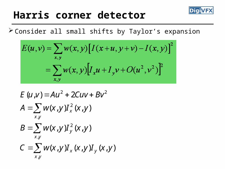
Consider all small shifts by Taylor’s expansion
yxyx
yxy
yxx
yxIyxIyxwC
yxIyxwB
yxIyxwA
BvCuvAuvuE
,
,
2
,
2
22
),(),(),(
),(),(
),(),(
2),(
Page 7
Harris corner detector
( , ) ,u
E u v u v Mv
Equivalently, for small shifts [u,v] we have a bilinear approximation:
2
2,
( , ) x x y
x y x y y
I I IM w x y
I I I
, where M is a 22 matrix computed from image derivatives:
Page 8
Visualize quadratic functions
10
01M
Page 9
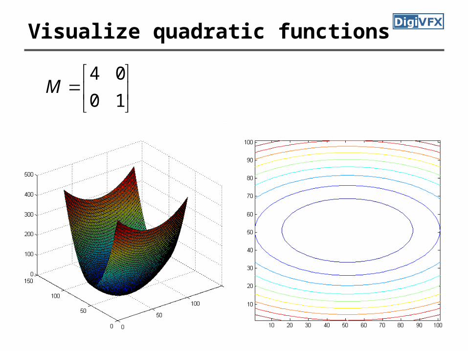
Visualize quadratic functions
10
04M
Page 10
Visualize quadratic functions
T
M
50.087.0
87.050.0
40
01
50.087.0
87.050.0
75.130.1
30.125.3
Page 11
Visualize quadratic functions
T
M
50.087.0
87.050.0
100
01
50.087.0
87.050.0
25.390.3
90.375.7
Page 12
Harris corner detector (matrix form)
xxx
xxx
xx
TT
T
T
III
II
I
2
2
00
Page 13
Harris corner detector
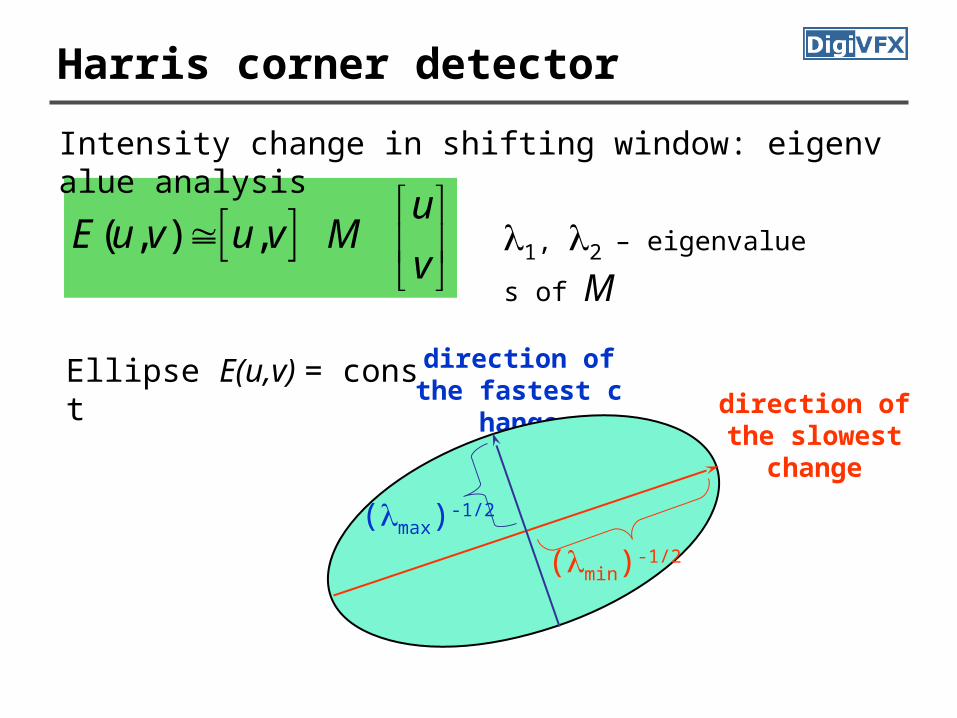
( , ) ,u
E u v u v Mv
Intensity change in shifting window: eigenvalue analysis
1, 2 – eigenvalues of M
direction of the slowest chan
ge
direction of the fastest change
(max)-1/2
(min)-1/2
Ellipse E(u,v) = const
Page 14
Harris corner detector
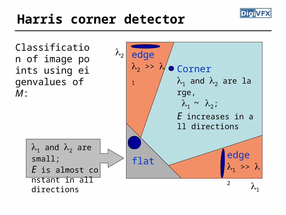
1
2
Corner1 and 2 are large,
1 ~ 2;
E increases in all directions
1 and 2 are small;
E is almost constant in all directions
edge 1 >> 2
edge 2 >> 1
flat
Classification of image points using eigenvalues of M:
Page 15
Harris corner detector
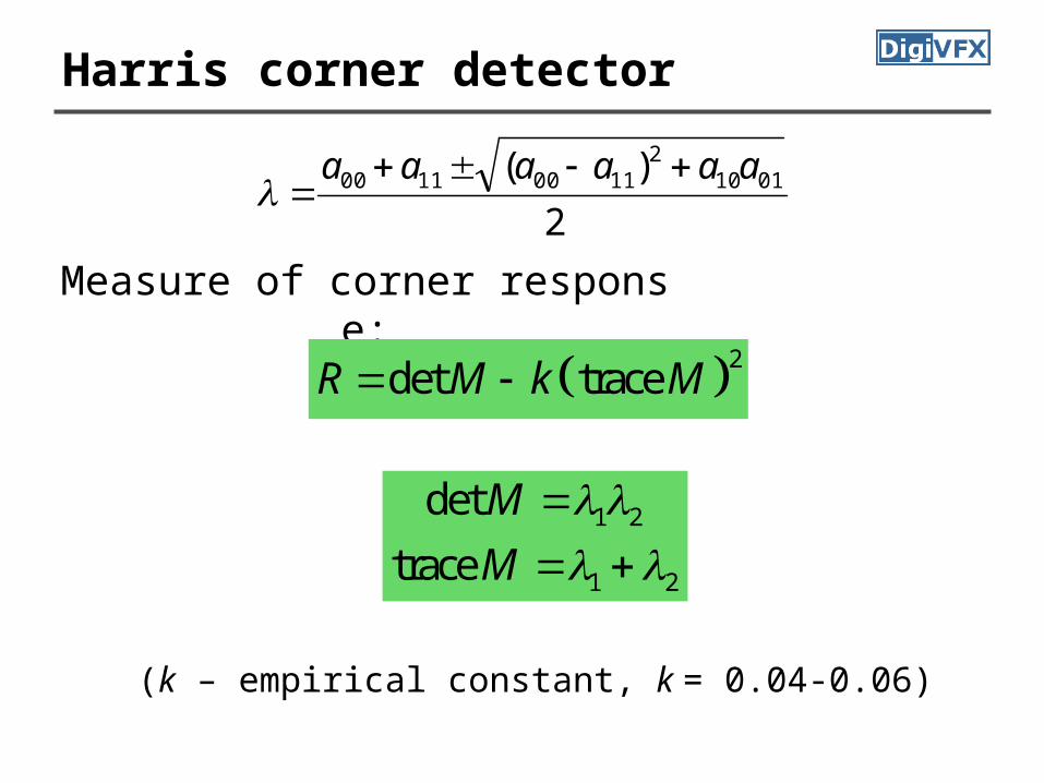
Measure of corner response:
2det traceR M k M
1 2
1 2
det
trace
M
M
(k – empirical constant, k = 0.04-0.06)
2
)( 01102
11001100 aaaaaa
Page 16
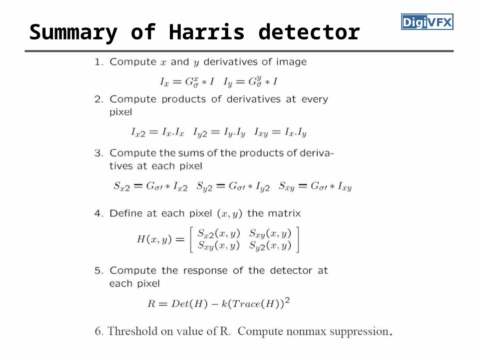
Summary of Harris detector
Page 17
Now we know where features are
• But, how to match them?• What is the descriptor for a feature? The
simplest solution is the intensities of its spatial neighbors. This might not be robust to brightness change or small shift/rotation.
Page 18
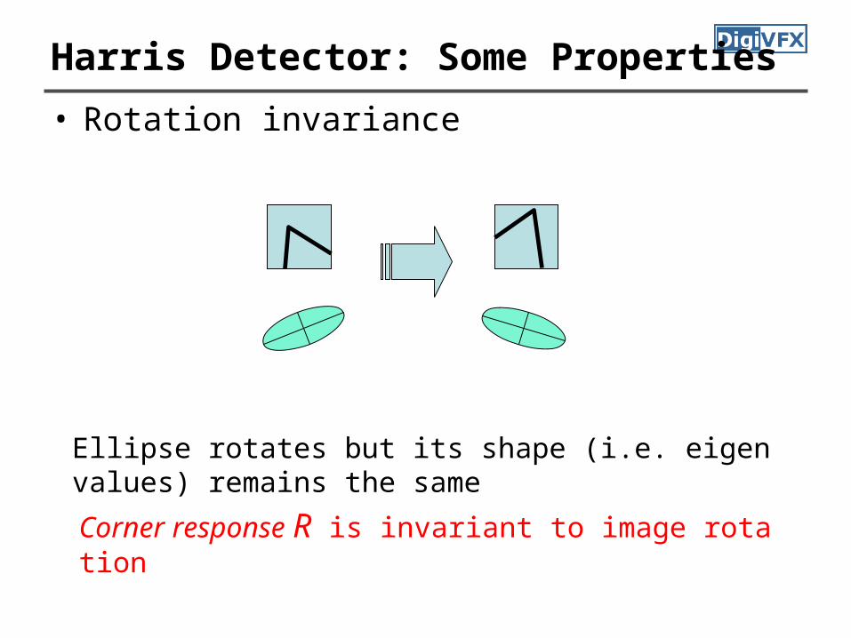
Harris Detector: Some Properties• Rotation invariance
Ellipse rotates but its shape (i.e. eigenvalues) remains the sameCorner response R is invariant to image rotation
Page 19
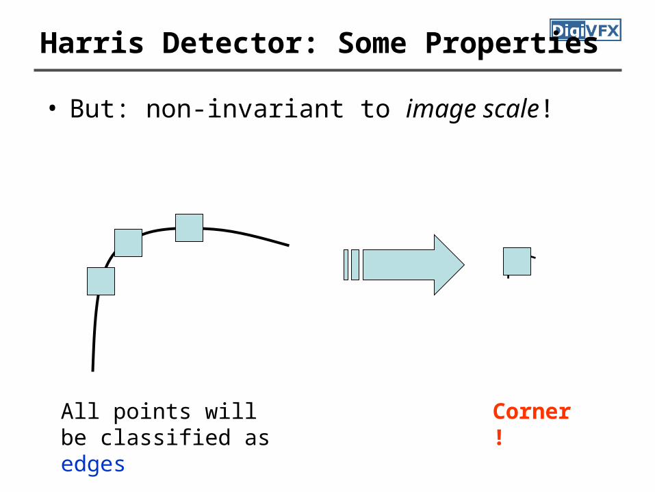
Harris Detector: Some Properties
• But: non-invariant to image scale!
All points will be classified as edges
Corner !
Page 20
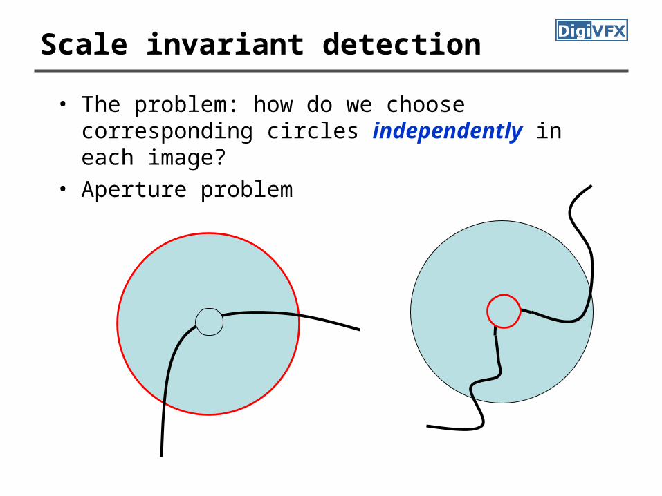
Scale invariant detection
• The problem: how do we choose corresponding circles independently in each image?
• Aperture problem
Page 21
SIFT (Scale Invariant Feature
Transform)
Page 22
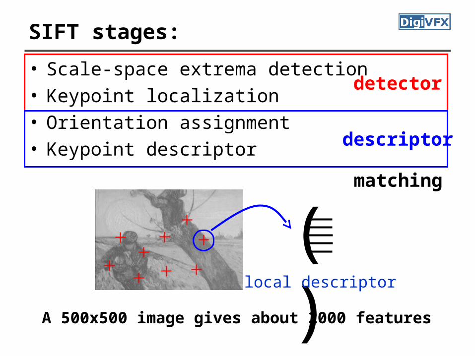
SIFT stages:
• Scale-space extrema detection• Keypoint localization• Orientation assignment• Keypoint descriptor
( )local descriptor
detector
descriptor
A 500x500 image gives about 2000 features
matching
Page 23
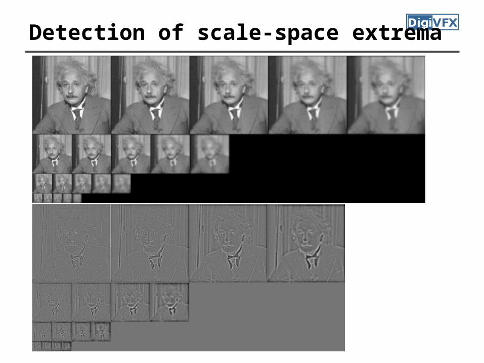
1. Detection of scale-space extrema• For scale invariance, search for stable features
across all possible scales using a continuous function of scale, scale space.
• SIFT uses DoG filter for scale space because it is efficient and as stable as scale-normalized Laplacian of Gaussian.
Page 24
Scale space doubles for the next octave
K=2(1/s)
Page 25
Detection of scale-space extrema
Page 26
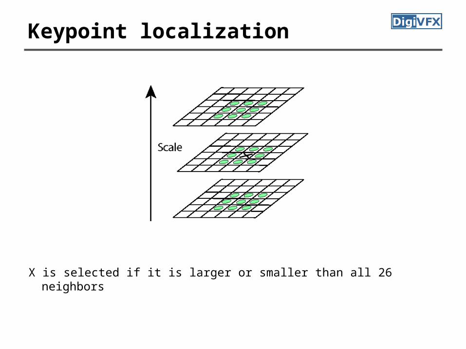
Keypoint localization
X is selected if it is larger or smaller than all 26 neighbors
Page 27
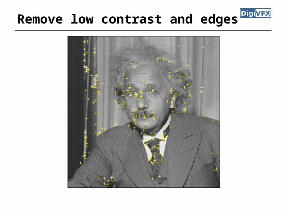
2. Accurate keypoint localization• Reject points with low contrast and poorly
localized along an edge• Fit a 3D quadratic function for sub-pixel
maxima
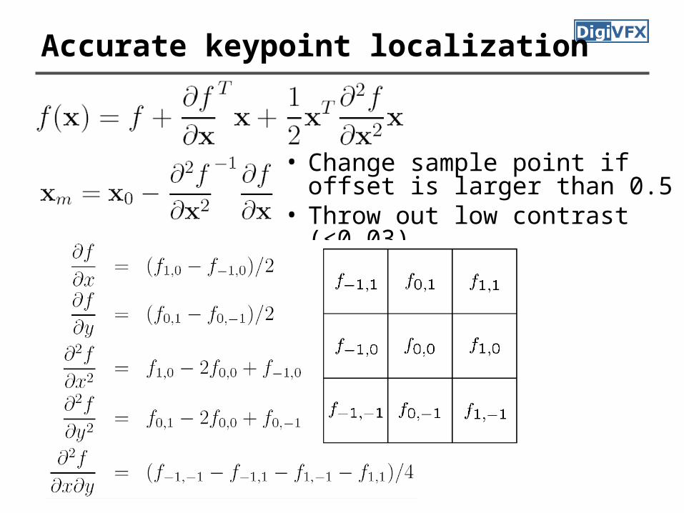
Page 28
Accurate keypoint localization
• Change sample point if offset is larger than 0.5
• Throw out low contrast (<0.03)
Page 29
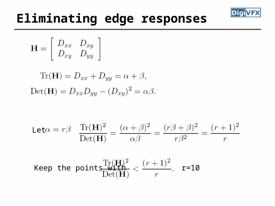
Eliminating edge responses
r=10
Let
Keep the points with
Page 31
Remove low contrast and edges
Page 32
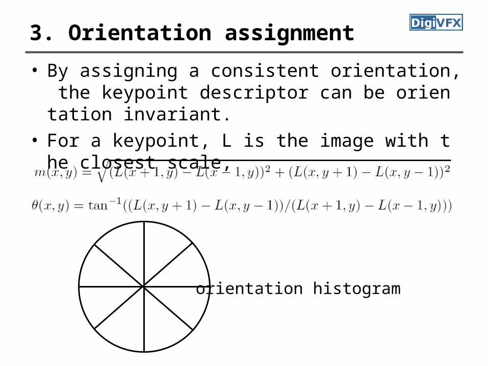
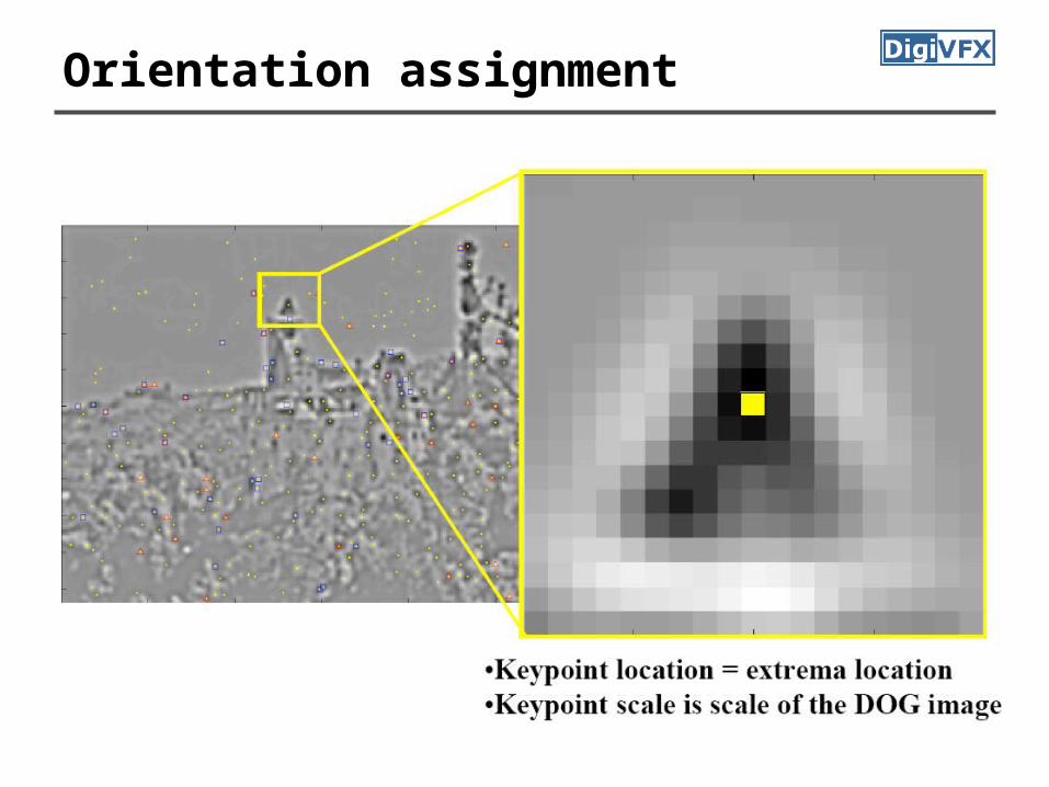
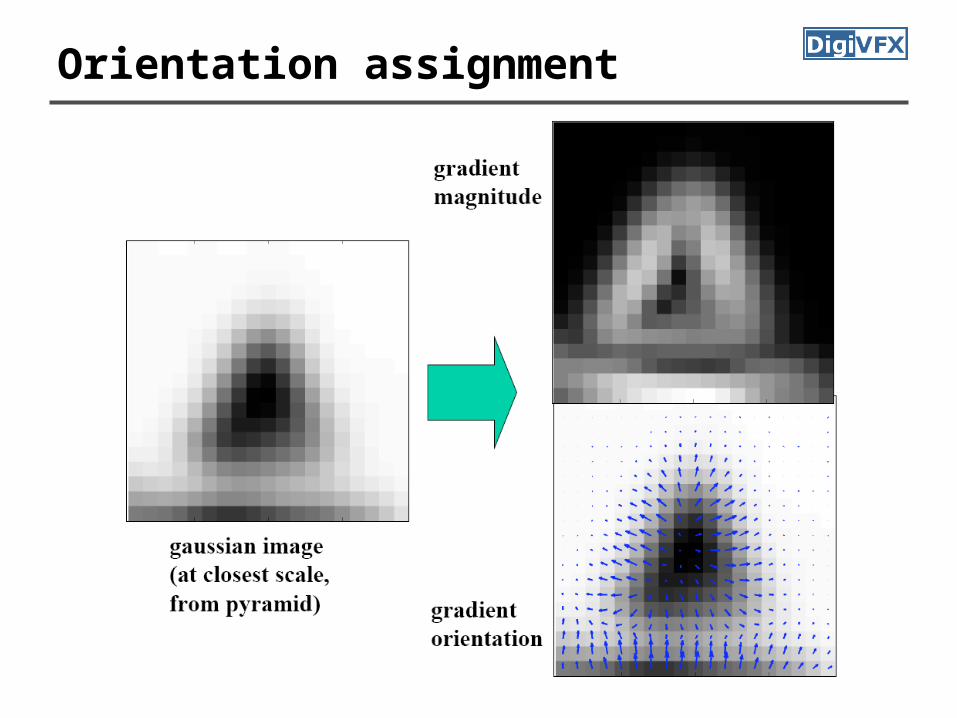
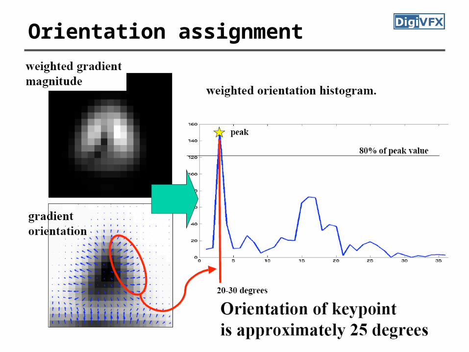
3. Orientation assignment
• By assigning a consistent orientation, the keypoint descriptor can be orientation invariant.
• For a keypoint, L is the image with the closest scale,
orientation histogram
Page 33
Orientation assignment
Page 34
Orientation assignment
Page 35
Orientation assignment
Page 36
Orientation assignment
Page 38
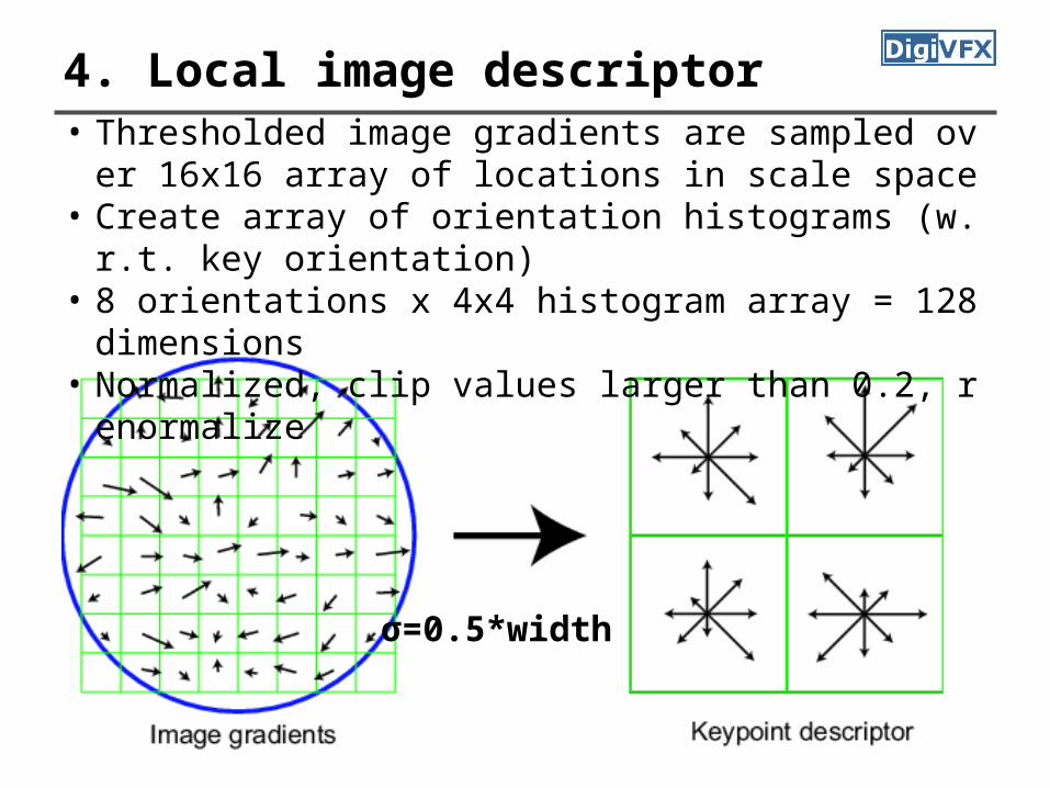
4. Local image descriptor• Thresholded image gradients are sampled over 16x16
array of locations in scale space• Create array of orientation histograms (w.r.t. key orie
ntation)• 8 orientations x 4x4 histogram array = 128 dimensions• Normalized, clip values larger than 0.2, renormalize
σ=0.5*width
Page 41
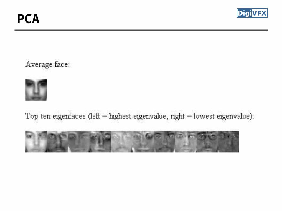
PCA-SIFT
• Only change step 4• Pre-compute an eigen-space for local gradient
patches of size 41x41• 2x39x39=3042 elements• Only keep 20 components• A more compact descriptor
Page 42
GLOH (Gradient location-orientation histogram)
17 location bins16 orientation binsAnalyze the 17x16=272-d eigen-space, keep 128 components
SIFT
Page 43
Multi-Scale Oriented Patches• Simpler than SIFT. Designed for image matchi
ng. [Brown, Szeliski, Winder, CVPR’2005]• Feature detector
– Multi-scale Harris corners– Orientation from blurred gradient– Geometrically invariant to rotation
• Feature descriptor– Bias/gain normalized sampling of local patch (8x8)– Photometrically invariant to affine changes in inten
sity
Page 44
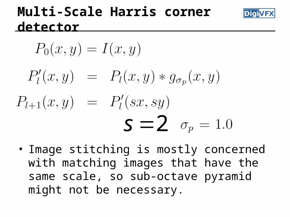
Multi-Scale Harris corner detector
• Image stitching is mostly concerned with matching images that have the same scale, so sub-octave pyramid might not be necessary.
2s
Page 45
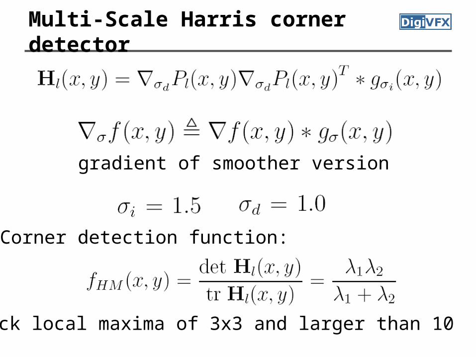
Multi-Scale Harris corner detector
gradient of smoother version
Corner detection function:
Pick local maxima of 3x3 and larger than 10
Page 46
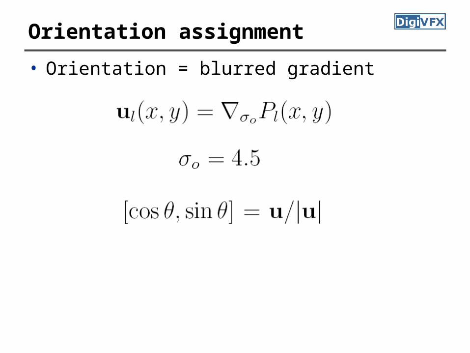
Orientation assignment
• Orientation = blurred gradient
Page 47
MOPS descriptor vector• Scale-space position (x, y, s) + orientation ()• 8x8 oriented patch sampled at 5 x scale. See th
e Technical Report for more details. • Bias/gain normalisation: I’ = (I – )/
8 pixels40 pixels
Page 48
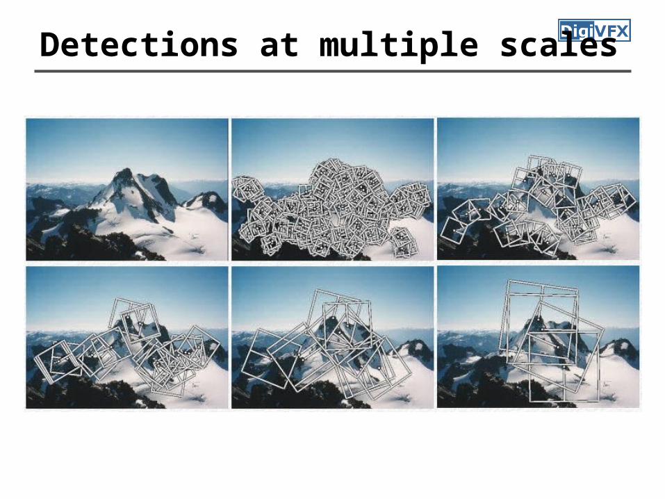
Detections at multiple scales
Page 49
Feature matching• Exhaustive search
– for each feature in one image, look at all the other features in the other image(s)
• Hashing– compute a short descriptor from each feature vect
or, or hash longer descriptors (randomly)• Nearest neighbor techniques
– k-trees and their variants (Best Bin First)
Page 50
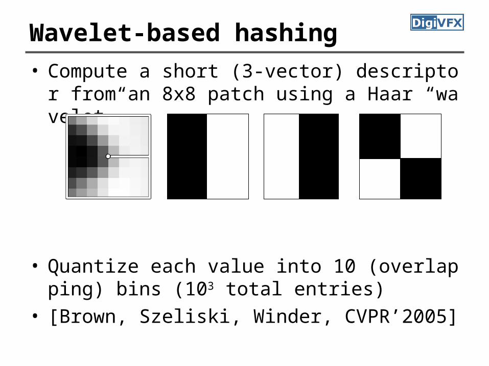
Wavelet-based hashing• Compute a short (3-vector) descriptor from an
8x8 patch using a Haar “wavelet”
• Quantize each value into 10 (overlapping) bins (103 total entries)
• [Brown, Szeliski, Winder, CVPR’2005]
Page 51
Nearest neighbor techniques• k-D tree
and
• Best BinFirst(BBF)
Indexing Without Invariants in 3D Object Recognition, Beis and Lowe, PAMI’99
Page 52
Reference
• Chris Harris, Mike Stephens, A Combined Corner and Edge Detector, 4th Alvey Vision Conference, 1988, pp147-151.
• David G. Lowe, Distinctive Image Features from Scale-Invariant Keypoints, International Journal of Computer Vision, 60(2), 2004, pp91-110.
• Yan Ke, Rahul Sukthankar, PCA-SIFT: A More Distinctive Representation for Local Image Descriptors, CVPR 2004.
• Krystian Mikolajczyk, Cordelia Schmid, A performance evaluation of local descriptors, Submitted to PAMI, 2004.
• SIFT Keypoint Detector, David Lowe.• Matlab SIFT Tutorial, University of Toronto.• Matthew Brown, Richard Szeliski, Simon Winder,
Multi-Scale Oriented Patches, MSR-TR-2004-133, 2004.