MORE RISK-SENSITIVE MARKOV DECISION PROCESSES

NICOLE BAUERLE∗ AND ULRICH RIEDER‡

Abstract. We investigate the problem of minimizing a certainty equivalent of the total ordiscounted cost over a finite and an infinite horizon which is generated by a Markov DecisionProcess (MDP). The certainty equivalent is defined by U−1(EU(Y )) where U is an increasingfunction. In contrast to a risk-neutral decision maker this optimization criterion takes thevariability of the cost into account. It contains as a special case the classical risk-sensitiveoptimization criterion with an exponential utility. We show that this optimization problemcan be solved by an ordinary MDP with extended state space and give conditions under whichan optimal policy exists. In the case of an infinite time horizon we show that the minimaldiscounted cost can be obtained by value iteration and can be characterized as the uniquesolution of a fixed point equation using a ’sandwich’ argument. Interestingly, it turns out thatin case of a power utility, the problem simplifies and is of similar complexity than the exponentialutility case, however has not been treated in the literature so far. We also establish the validity(and convergence) of the policy improvement method. A simple numerical example, namely theclassical repeated casino game is considered to illustrate the influence of the certainty equivalentand its parameters. Finally also the average cost problem is investigated. Surprisingly it turnsout that under suitable recurrence conditions on the MDP for convex power utility U , theminimal average cost does not depend on U and is equal to the risk neutral average cost. Thisis in contrast to the classical risk sensitive criterion with exponential utility.

Key words: Markov Decision Problem, Certainty Equivalent, Positive HomogeneousUtility, Exponential Utility, Value Iteration, Policy Improvement, Risk-sensitive Av-erage Cost.

AMS subject classifications: 90C40, 91B06.

1. Introduction

Since the seminal paper by Howard & Matheson (1972) the notion risk-sensitive Markov DecisionProcess (MDP) seems to be reserved for the criterion 1

γ logE[eγY ] where Y is some cumulated

cost and γ represents the degree of risk aversion or risk attraction. However in the recent decadea lot of alternative ways of measuring performance with a certain emphasis on risk arose. Amongthem risk measures and the well-known certainty equivalents. Certainty equivalents have a longtradition and its use can be traced back to the 1930ies (for a historic review see Muliere &Parmigiani (1993)). They are defined by U−1(EU(Y )) where U is an increasing function. Weconsider here a discrete-time MDP evolving on a Borel state space which accumulates cost overa finite or an infinite time horizon. The one-stage cost are bounded. The aim is to minimizethe certainty equivalent of this accumulated cost. In case of an infinite time horizon, cost haveto be discounted. We will also consider an average cost criterion.

The problems we treat here are generalizations of the classical ’risk-sensitive’ case which isobtained when we set U(y) = 1

γ eγy. On the other hand they are more specialized than the

problems with expected utility considered for example in Kreps (1977a,b). There the authorconsiders a countable state, finite action MDP where the utility which has to be maximized maydepend on the complete history of the process. In such a setting it is already hard to obtainsome kind of stationarity. It is achieved by introducing what the author calls a summary space- an idea which is natural and which will also appear in our analysis. A forward recursive utilityand its summary (which is there called forward recursive accumulation) are investigated for afinite horizon problem in Iwamoto (2004).

c©0000 (copyright holder)

1

2 N. BAUERLE AND U. RIEDER

Somehow related studies can be found in Jaquette (1973, 1976) where finite state, finiteaction MDPs are considered and moment optimality and the exponential utility of the infinitehorizon discounted reward is investigated. General optimization criteria can also be found inChung & Sobel (1987). There the authors first consider fixed point theorems for the completedistribution of the infinite horizon discounted reward in a finite MDP and later also consider theexponential utility. In Collins & McNamara (1998) the authors deal with a finite horizon problemand maximize a strictly concave functional of the distribution of the terminal state. Anothernon-standard optimality criterion is the target level criterion where the aim is to maximizethe probability that the total discounted reward exceeds a given target value. This is e.g.investigated in Wu & Lin (1999); Boda et al. (2004). Other probabilistic criteria, mostly incombination with long-run performance measures, can be found in the survey of White (1988).

Only recently some papers appeared where risk measures have been used for optimizationof MDPs. In Ruszczynski (2010) general space MDPs are considered in a finite horizon modelas well as in a discounted infinite horizon model. A dynamic Markov risk measure is usedas optimality criterion. In both cases value iteration procedures are established and for theinfinite horizon model the validity and convergence of the policy improvement method is shown.The concrete risk measure Average-Value-at-Risk has been used in Bauerle & Ott (2011) forminimizing the discounted cost over a finite and an infinite horizon for a general state MDP. Valueiteration methods have been established and the optimality of Markov policies depending on acertain ’summary’ has been shown. Some numerical examples have also been given, illustratingthe influence of the ’risk aversion parameter’. In Bauerle & Mundt (2009) a Mean-Average-Value-at-Risk problem has been solved for an investor in a binomial financial market.

Classical risk-sensitive MDPs have been intensively studied since Howard & Matheson (1972).In particular the average cost criterion has attracted a lot of researchers since it behaves con-siderable different to the classical risk neutral average cost problem (see e.g. Cavazos-Cadena& Hernandez-Hernandez (2011); Cavazos-Cadena & Fernandez-Gaucherand (2000); Jaskiewicz(2007); Di Masi & Stettner (1999)). The infinite horizon discounted classical risk-sensitive MDPand its relation to the average cost problem is considered in Di Masi & Stettner (1999). As faras applications are concerned, risk-sensitive problems can e.g. be found in Bielecki et al. (1999)where portfolio management is considered, in Denardo et al. (2011, 2007) where multi-armedbandits are investigated and in Barz & Waldmann (2007) where revenue problems are treated.

In this paper we investigate the problem of minimizing the certainty equivalent of the total anddiscounted cost over a finite and an infinite horizon which is generated by a Markov DecisionProcess. We consider both the risk averse and the risk seeking case. We show that theseproblems can be solved by ordinary MDPs with extended state space and give continuity andcompactness conditions under which optimal policies exist. In the case of discounting we haveto enlarge the state space by another component since the discount factor implies some kindof non-stationarity. The enlargement of the state space is partly dispensable for exponential orpower utility functions. Interestingly, the problem with power utility shows a similar complexitythan the classical exponential case, but to the best of our knowledge has not been considered inthe MDP literature so far. In the case of an infinite horizon we show that the minimal value canbe obtained by value iteration and can be characterized as the unique solution of a fixed pointequation using a ’sandwich’ argument. We also establish the validity (and convergence) of thepolicy improvement method. A simple numerical example, namely a classical repeated casinogame, is considered to illustrate the influence of the function U and its parameters. Finally alsothe average cost problem is investigated. Surprisingly it turns out that under suitable recurrenceconditions on the MDP for U(y) = 1

γ yγ with γ ≥ 1, the minimal average cost does not depend

on γ and are equal to the risk neutral average cost. This is in contrast to the classical risksensitive criterion. The average cost case with γ < 1 remains an open problem.

The paper is organized as follows: In Section 2 we introduce the MDP model, our continuityand compactness assumptions and the admissible policies. In Section 3 we solve the finite horizonproblem with certainty equivalent criterion. We consider the total cost problem as well as the

MORE RISK-SENSITIVE MARKOV DECISION PROCESSES 3

discounted cost problem. In the latter case we have to further extend the state space of the MDP.One subsection deals with the repeated casino game which is solved explicitly. Next, in Section4 we consider and solve the infinite horizon problem. We show that the minimal discountedcost can be obtained by value iteration and can be characterized as the unique solution of afixed point equation. We also establish the validity (and convergence) of the policy improvementmethod. Finally in Section 5 we investigate the average cost problem for power utility.

2. General Risk-Sensitive Markov Decision Processes

We suppose that a controlled Markov state process (Xn) in discrete time is given with values ina Borel set E. More precisely it is specified by:

• The Borel state space E, endowed with a Borel σ-algebra E .• The Borel action space A, endowed with a Borel σ-algebra A.• The set D ⊂ E × A, a nonempty Borel set and subsets D(x) := {a ∈ A : (x, a) ∈ D} of

admissible actions in state x.• A regular conditional distribution Q from D to E, the transition law.• A measurable cost function c : D → [c, c] with 0 < c < c.

Note that we assume here for simplicity that the cost are positive and bounded. Next weintroduce the sets of histories for k ∈ N by:

H0 := E, Hn := Dn × E

where hn = (x0, a0, x1, . . . , an−1, xn) ∈ Hn gives a history up to time n. A history-dependentpolicy σ = (gn)n∈N0 is given by a sequence of measurable mappings gn : Hn → A such thatgn(hn) ∈ D(xn). We denote the set of all such policies by Π. Each policy σ ∈ Π inducestogether with the initial state x a probability measure Pσx and a stochastic process (Xn, An) onH∞ such that Xn is the random state at time n and An is the action at time n. (For details seee.g. Bauerle & Rieder (2011), Section 2).

There is a discount factor β ∈ (0, 1] and we will either consider a finite planning horizonN ∈ N0 or an infinite planning horizon. Thus we will either consider the cost

CNβ :=N−1∑k=0

βkc(Xk, Ak) or C∞β :=∞∑k=0

βkc(Xk, Ak).

If β = 1 we will shortly write CN instead of CN1 . In the last section we will also consider averagecost problems. Instead of minimizing the expected cost we will now treat a general non-standardrisk-sensitive criterion. To this end let U be a continuous and strictly increasing function suchthat the inverse U−1 exists. The aim now is to solve:

infσ∈Π

U−1(Eσx[U(CNβ )

]), x ∈ E, (2.1)

infσ∈Π

U−1(Eσx[U(C∞β )

]), x ∈ E (2.2)

where Eσx is the expectation w.r.t. Pσx. Note that the problems in (2.1) and (2.2) are well-defined.

If U is in addition strictly convex, then the quantity U−1(E[U(Y )

])can be interpreted as the

mean-value premium of the risk Y as is done in actuarial sciences (see e.g. Kaas et al. (2009)).If U is strictly concave, then U is a utility function and the quantity represents a certaintyequivalent also known as a quasi-linear mean. It may be written (assuming enough regularity ofU) using the Taylor rule as

U−1(E[U(Y )

])≈ EY − 1

2lU (EY )V ar[Y ]

where

lU (y) = −U′′(y)

U ′(y)

4 N. BAUERLE AND U. RIEDER

is the Arrow-Pratt function of absolute risk aversion. Hence the second term accounts for thevariability of X (for a discussion see Bielecki & Pliska (2003)). If U is concave, the varianceis subtracted and hence the decision maker is risk seeking in case cost are minimized, if U isconvex, then the variance is added and the decision maker is risk averse. A prominent specialcase is the choice

U(y) =1

γeγy, γ 6= 0

in which case lU (y) = −γ. When we speak of minimizing cost, the case γ > 0 corresponds to arisk averse decision maker and the case γ < 0 to a risk-seeking decision maker. Note that thisinterpretation changes when we maximize reward. The limiting case γ → 0 coincides with theclassical risk-neutral criterion.

Other interesting choices are U(y) = 1γ y

γ with γ > 0. For γ < 1 the function U is strictly

concave and lU (y) = 1−γy . This is the risk-seeking case for the cost problem. If γ ≥ 1 we can

also write

U−1(E[U(Y )]

)=(EY γ

) 1γ

= ‖Y ‖γ

where ‖ · ‖γ is the usual Lγ-norm. Of course γ = 1 is again the risk neutral case.In this paper we impose the following continuity and compactness assumptions (CC) on the

data of the problem:

(i) U : [0,∞)→ R is continuous and strictly increasing,(ii) D(x) is compact for all x ∈ E,(iii) x 7→ D(x) is upper semicontinuous, i.e. for all x ∈ E it holds: If xn → x and an ∈ D(xn)

for all n ∈ N, then (an) has an accumulation point in D(x),(iv) (x, a) 7→ c(x, a) is lower semicontinuous,(v) Q is weakly continuous, i.e. for a all v : E → R bounded and continuous

(x, a) 7→∫v(x′)Q(dx′|x, a)

is again continuous.

Note that assumptions (CC) will later imply the existence of optimal policies and the validityof the value iteration. It is also possible to show these statements under other assumptions, inparticular under so-called structure assumptions. For a discussion see e.g. Bauerle & Rieder(2011), Section 2.4.

3. Finite Horizon Problems

3.1. Total Cost Problems. We start investigating the case of a finite time horizon N andβ = 1. Since U is strictly increasing, so is U−1 and we can obviously skip it from the optimizationproblem. In what follows we denote by

JN (x) := infσ∈Π

Eσx[U(N−1∑k=0

c(Xk, Ak))]

= infσ∈Π

Eσx[U(CN )], x ∈ E. (3.1)

Though this problem is not directly separable, we will show that it can be solved by a bivariateMDP as follows. For this purpose let us define for n = 0, 1, . . . , N

Vnσ(x, y) := Eσx[U(Cn + y

)], x ∈ E, y ∈ R+, σ ∈ Π,

Vn(x, y) := infσ∈Π

Vnσ(x, y), x ∈ E, y ∈ R+. (3.2)

Obviously VN (x, 0) = JN (x). The idea is that y summarizes the cost which has been accumulatedso far. This idea can already be found in Kreps (1977a,b). We consider now a Markov Decision

Model which is defined on the state space E := E × R+ with action space A and admissible

MORE RISK-SENSITIVE MARKOV DECISION PROCESSES 5

actions given by the set D. The one-stage cost are zero and the terminal cost function isV0(x, y) := U(y). The transition law is given by Q(·|x, y, a) defined by∫

v(x′, y′)Q(d(x′, y′)|x, y, a) =

∫v(x′, c(x, a) + y)Q(dx′|x, a).

Decision rules are here given by measurable mappings f : E → A such that f(x, y) ∈ D(x). Wedenote by F the set of decision rules and by ΠM the set of Markov policies π = (f0, f1, . . .) withfn ∈ F . Note that ‘Markov’ refers to the fact that the decision at time n depends only on xand y. Obviously in (3.2) only the first n decision rules of σ are relevant. Note that we haveΠM ⊂ Π in the following sense: For every π = (f0, f1, . . .) ∈ ΠM we find a σ = (g0, g1, . . .) ∈ Πsuch that

g0(x0) := f0(x0, 0),

gn(x0, a0, x1, . . . , xn) := fn(xn,

n−1∑k=0

c(xk, ak)), n ∈ N.

With this interpretation Vnπ is also defined for π ∈ ΠM . For convenience we introduce the set

C(E) :={v : E → R : v is lower semicontinuous, v(x, ·)is continuous

and increasing for x ∈ E and v(x, y) ≥ U(y)}.

Note that v ∈ C(E) is bounded from below. For v ∈ C(E) and f ∈ F we denote the operator

(Tfv)(x, y) :=

∫v(x′, c(x, f(x, y)) + y

)Q(dx′|x, f(x, y)

), (x, y) ∈ E.

The minimal cost operator of this Markov Decision Model is given by

(Tv)(x, y) = infa∈D(x)

∫v(x′, c(x, a) + y

)Q(dx′|x, a

), (x, y) ∈ E. (3.3)

If a decision rule f ∈ F is such that Tfv = Tv, then f is called a minimizer of v. In what followswe will always assume that the empty sum is zero. Then we obtain:

Theorem 3.1. It holds that

a) For a policy π = (f0, f1, f2, . . .) ∈ ΠM we have the following cost iteration:Vnπ = Tf0 . . . Tfn−1U for n = 1, . . . , N .

b) V0(x, y) := U(y) and Vn = TVn−1, for n = 1, . . . , N i.e.

Vn(x, y) = infa∈D(x)

∫Vn−1

(x′, c(x, a) + y

)Q(dx′|x, a

).

Moreover, Vn ∈ C(E).c) For every n = 1, . . . , N there exists a minimizer f∗n ∈ F of Vn−1 and (g∗0, . . . , g

∗N−1) with

g∗n(hn) := f∗N−n(xn,

n−1∑k=0

c(xk, ak)), n = 0, . . . , N − 1

is an optimal policy for problem (3.1). Note that the optimal policy consists of decisionrules which depend on the current state and the accumulated cost so far.

Proof. We will first prove part a) by induction. By definition V0π(x, y) = U(y) and

V1π(x, y) = U(c(x, f0(x, y)) + y

)= (Tf0U)(x, y).

6 N. BAUERLE AND U. RIEDER

Now suppose the statement holds for Vn−1π and consider Vnπ. In order to ease notation wedenote for a policy π = (f0, f1, f2, . . .) ∈ ΠM by ~π = (f1, f2, . . .) the shifted policy. Hence

(Tf0 . . . Tfn−1U)(x, y) =

∫Vn−1~π

(x′, c(x, f0(x, y)) + y

)Q(dx′|x, f0(x, y))

=

∫E~πx′[U( n−2∑k=0

c(Xk, Ak) + c(x, f0(x, a)) + y)]Q(dx′|x, f0(x, a))

= Vnπ(x, y).

Next we prove part b) and c) together. From part a) it follows that for π ∈ ΠM , the valuefunctions in problem (3.2) indeed coincide with the value functions of the previously definedMDP. From MDP theory it follows in particular that it is enough to consider Markov policiesΠM , i.e. Vn = infσ∈Π Vnσ = infπ∈ΠM Vnπ (see e.g. Hinderer (1970) Theorem 18.4). Next

consider functions v ∈ C(E). We show that Tv ∈ C(E) and that there exists a minimizer for v.Statements b) and c) then follow from Theorem 2.3.8 in Bauerle & Rieder (2011).

Now suppose v ∈ C(E). Taking into account our standing assumptions (CC) (i),(iv) at theend of section 2 it obviously follows that (x, y, a, x′) 7→ v

(x′, c(x, a)+y

)is lower semicontinuous.

Moreover y 7→ v(x′, c(x, a) + y

)is increasing and continuous. We can now apply Theorem 17.11

in Hinderer (1970) to obtain that (x, y, a) 7→∫v(x, y, a, x′)Q(dx′|x, a) is lower semicontinuous.

By Proposition 2.4.3 in Bauerle & Rieder (2011) it follows that (x, y) 7→ (Tv)(x, y) is lowersemicontinuous and there exists a minimizer of v.

Further it is clear that y 7→∫v(x′, c(x, a) + y

)Q(dx′|x, a) is increasing and continuous (by

monotone convergence), i.e. in particular upper semicontinuous. Now since the infimum ofan arbitrary number of upper semicontinuous functions is upper semicontinuous, we obtainy 7→ (Tv)(x, y) is continuous and also increasing. The inequality (Tv)(x, y) ≥ U(y) followsdirectly. �

The last theorem shows that the optimal policy of (3.1) can be found in the smaller set ΠM

which makes the problem computationally tractable.In the special case U(y) = 1

γ eγy with γ 6= 0 the iteration simplifies and the second component

can be skipped.

Corollary 3.2 (Exponential Utility). In case U(y) = 1γ e

γy with γ 6= 0, we obtain

a) Vn(x, y) = eγyhn(x), n = 0, . . . , N and JN (x) = hN (x).b) The functions hn from part a) are given by h0 = 1

γ and

hn(x) = infa∈D(x)

{eγc(x,a)

∫hn−1(x′)Q(dx′|x, a)

}.

Proof. We prove the statements a) and b) by induction. For n = 0 we obtain V0(x, y) = 1γ e

γy =

eγy · 1γ , hence h0 ≡ 1

γ . Now suppose part a) is true for n − 1. From the Bellman equation

(Theorem 3.1 b)) we obtain:

Vn(x, y) = infa∈D(x)

∫Vn−1

(x′, c(x, a) + y

)Q(dx′|x, a

)= inf

a∈D(x)

∫eγ(y+c(x,a))hn−1(x′)Q

(dx′|x, a

)= eγy inf

a∈D(x)

{eγc(x,a)

∫hn−1(x′)Q

(dx′|x, a

)}.

Hence the statement follows by setting hn(x) = infa∈D(x)

{eγc(x,a)

∫hn−1(x′)Q(dx′|x, a)

}. �

MORE RISK-SENSITIVE MARKOV DECISION PROCESSES 7

Remark 3.3. Taking the logarithm in the equation of part b) we obtain the maybe morefamiliar form

log hn(x) = infa∈D(x)

{γc(x, a) + log

∫hn−1(x′)Q(dx′|x, a)

}see e.g. Bielecki et al. (1999).

Remark 3.4. Of course instead of minimizing cost one could also consider the problem ofmaximizing reward. Suppose that r : D → [r, r] (with 0 < r < r) is a one-stage reward functionand the problem is

JN (x) := supσ∈Π

Eσx[U(N−1∑k=0

r(Xk, Ak))], x ∈ E. (3.4)

It is possible to treat this problem in exactly the same way. The value iteration is given byV0(x, y) := U(y) and

Vn(x, y) = supa∈D(x)

∫Vn−1

(x′, r(x, a) + y

)Q(dx′|x, a

).

Remark 3.5. It is possible to state similar results for models where the cost does also dependon the next state, i.e. c = c(Xk, Ak, Xk+1). In particular, the value iteration reads here

Vn(x, y) = infa∈D(x)

∫Vn−1

(x′, y + c(x, a, x′)

)Q(dx′|x, a

).

Note however, that for exponential utility we have to modify the iteration in Corollary 3.2accordingly.

3.2. Application: Casino Game. In this section, we are going to illustrate the results of theprevious section and the influence of the choice of the function U by means of a simple numericalexample. For the given horizon N ∈ N, we consider N independent identically distributed games.The probability of winning one game is given by p ∈ (0, 1). We assume that the gambler startswith initial capital x0 > 0. Further, let Xk−1, k = 1, . . . , N , be the capital of the gambler rightbefore the k-th game. The final capital is denoted by XN . Before each game, the gambler hasto decide how much capital she wants to bet in the following game in order to maximize herrisk-adjusted profit. The aim is to find

JN (x0) := supσ∈Π

Eσx[U(XN )

], x0 > 0. (3.5)

This is obviously a reward maximization problem, but can be treated by the same means (seeRemark 3.4). As one-stage reward we choose r(Xk, Ak, Xk+1) = Xk+1 − Xk. Note that herethe reward depends on the outcome of the next state (see Remark 3.5). In what follows we willdistinguish between two cases: In the first one we choose U(y) = yγ for γ > 0 and in the secondone U(y) = 1

γ eγy for γ 6= 0. Let us denote by Z1, . . . , ZN independent and identically distributed

random variables which describe the outcome of the games. More precisely, Zk = 1 if the k-thgame is won and Zk = −1 if the k-th game is lost. Let us denote by QZ the distribution of Z.

Case 1: Let U(y) = yγ with γ > 0. Since the games are independent it is not difficult tosee that in this case we do not need the artificial state variable y or can identify x and y whenwe choose x to be the current capital (=accumulated reward). Moreover, it is reasonable todescribe the action in terms of the fraction of money that the gambler bets. Hence E := R+ andA = [0, 1] where D(x) = A. We obtain Xk+1 = Xk + XkAkZk+1 and hence r(Xk, Ak, Xk+1) =Xk+1 −Xk = XkAkZk+1. The value iteration is given by

Vn(x) = supa∈[0,1]

∫Vn−1

(x+ xaz

)QZ(dz).

8 N. BAUERLE AND U. RIEDER

We have to start the iteration with V0(x) := xγ and are interested in obtaining VN (x0). It iseasy to see by induction that Vn(x) = xγdn for some constants dn and all one-stage optimizationproblems reduce to

supa∈[0,1]

∫(1 + az)γQZ(dz) = sup

a∈[0,1]

{p(1 + a)γ + (1− p)(1− a)γ

}. (3.6)

Hence the optimal fraction to bet does not depend on the time horizon nor on the current cap-ital. Depending on γ the optimal policy can be discussed explicitly.

Case γ = 1: : This is the risk neutral case. The function in (3.6) reduces to the linearfunction 1 + a(2p− 1). Obviously the optimal policy is f∗n(x) = 1 if p > 1

2 and f∗n(x) = 0

if p ≤ 12 . If p = 1

2 all policies are optimal.Case γ > 1: : This is the risk-seeking case. The function which has to be maximized in

(3.6) is convex on [0, 1] hence the maximum points are on the boundary of the interval.We obtain f∗(x) = 1 if p > 1

2γ and f∗(x) = 0 if p ≤ 12γ .

Case γ < 1: : This is the risk-averse case. We can find the maximum point of the functionin (3.6) by inspecting its derivative. We obtain (let us denote ρ = 1−p

p )

f∗(x) =ρ

1γ−1 − 1

1 + ρ1

γ−1

if p > 12 and f∗(x) = 0 if p ≤ 1

2 .

An illustration of the optimal policy can be seen in figure 1. There, the optimal fraction ofthe wealth which should be bet is plotted for different parameters γ. The red line is γ = 1

2and belongs to the risk neutral gambler. The green line belongs to γ = 2 and represents arisk seeking gambler. She will bet all her capital as soon as p > 1

4 . The other three non-linear

curves belong to risk averse gamblers with γ = 23 ,

12 ,

13 respectively. The smaller γ, the lower

the fraction which will be bet. The limiting case γ → 0 corresponds to the logarithmic utilityU(y) = log(y). In this case we have to maximize

supa∈[0,1]

{p log(1 + a) + (1− p) log(1− a)

}and the optimal policy is given by f∗n(x) = 0 if p ≤ 1

2 and f∗n(x) = 2p− 1 for p > 12 .

Case 2: Let U(y) = 1γ e

γy with γ 6= 0. Here we describe the action in terms of the amount

of money that the gambler bets. Hence E := R+ and A = R+ where D(x) = [0, x]. We obtainXk+1 = Xk +AkZk+1. The value iteration is given by

Vn(x) = supa∈[0,x]

∫Vn−1

(x+ az

)QZ(dz).

We have to start the iteration with V0(x) := 1γ e

γx and are interested in obtaining VN (x0). The

solution is more complicated in this case. We distinguish between γ < 0 and γ > 0:

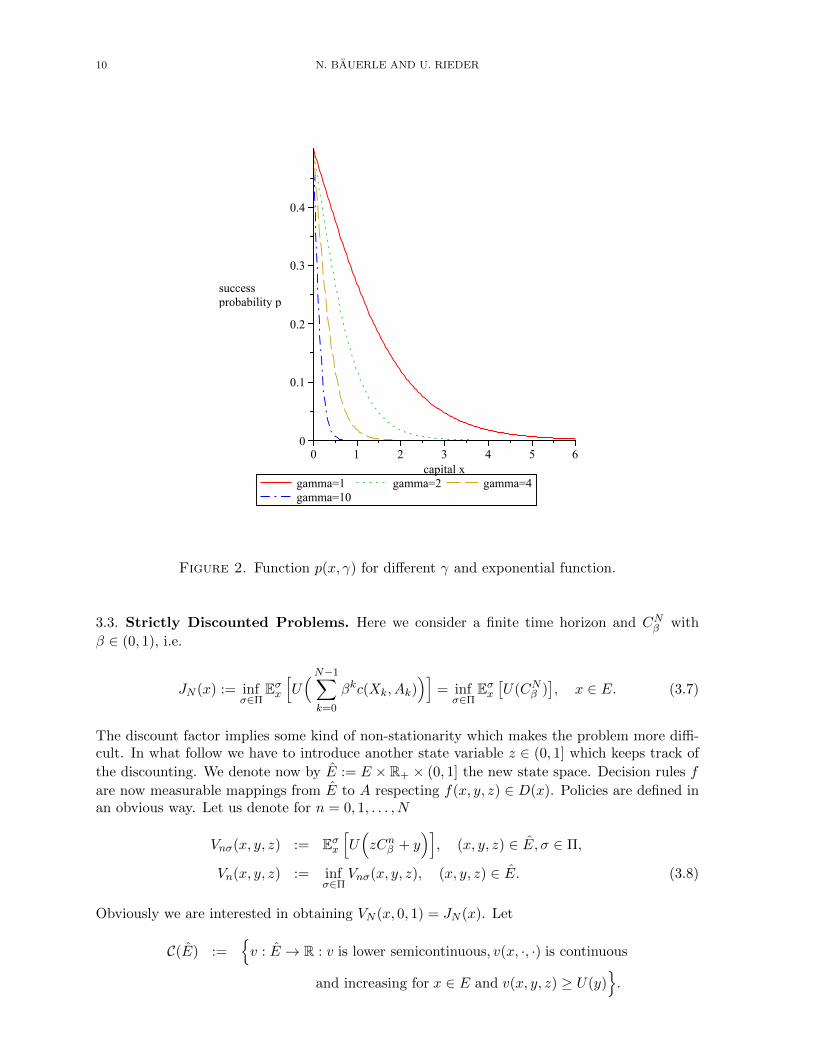
Case γ > 0: : This is the risk-seeking case. It follows from Proposition 2.4.21 in Bauerle& Rieder (2011) that the value functions are convex and hence a bang-bang policy isoptimal. We compute the optimal stake f∗1 (x) for one game. It is given by

f∗1 (x) =

{0 if p ≤ 1−e−γx

eγx−e−γx =: p(x, γ),

x else.

Note that the critical level p(x, γ) has the following properties:

0 ≤ p(x, γ) ≤ 1

2

limx→∞

p(x, γ) = 0, and limx→0

p(x, γ) =1

2

MORE RISK-SENSITIVE MARKOV DECISION PROCESSES 9

Figure 1. Optimal fractions of wealth to bet in the case of power utility withdifferent γ.

which means that a gambler with low capital will behave approximately as a risk neutralgambler and someone with a large capital will stake the complete capital even when theprobability of winning is quite small. Similarly

limγ→∞

p(x, γ) = 0, and limγ→0

p(x, γ) =1

2

i.e. if the gambler is more risk-seeking (γ large), she will stake her whole capital evenfor small success probabilities. The limiting case γ = 0 corresponds to the risk neutralgambler. In figure 2 the areas below the lines show the combinations of success probabilityand capital where it is optimal to bet nothing, depending on different values of γ. It canbe seen that this area gets smaller for larger γ, i.e. when the gambler is more risk-seeking.

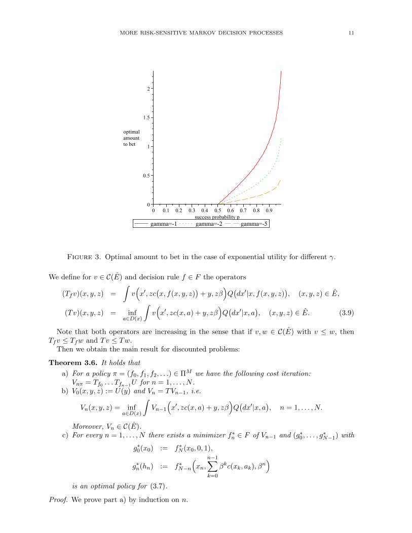
Case γ < 0: : This is the risk-averse case. In order to obtain a simple solution we allow thegambler to take a credit, i.e. E = R and A = R+, but the stake must be non-negative.In this setting we obtain an optimal policy where decisions are independent of the timehorizon and given by

f∗n(x) =

{0 if p ≤ 1

2 ,− 1

2γ log(p/(1− p)

)else.

The optimal amount to bet for different γ can be seen in figure 3. The smaller γ, thelarger the risk aversion and the smaller the amount to bet.

10 N. BAUERLE AND U. RIEDER

Figure 2. Function p(x, γ) for different γ and exponential function.

3.3. Strictly Discounted Problems. Here we consider a finite time horizon and CNβ with

β ∈ (0, 1), i.e.

JN (x) := infσ∈Π

Eσx[U(N−1∑k=0

βkc(Xk, Ak))]

= infσ∈Π

Eσx[U(CNβ )

], x ∈ E. (3.7)

The discount factor implies some kind of non-stationarity which makes the problem more diffi-cult. In what follow we have to introduce another state variable z ∈ (0, 1] which keeps track of

the discounting. We denote now by E := E × R+ × (0, 1] the new state space. Decision rules f

are now measurable mappings from E to A respecting f(x, y, z) ∈ D(x). Policies are defined inan obvious way. Let us denote for n = 0, 1, . . . , N

Vnσ(x, y, z) := Eσx[U(zCnβ + y

)], (x, y, z) ∈ E, σ ∈ Π,

Vn(x, y, z) := infσ∈Π

Vnσ(x, y, z), (x, y, z) ∈ E. (3.8)

Obviously we are interested in obtaining VN (x, 0, 1) = JN (x). Let

C(E) :={v : E → R : v is lower semicontinuous, v(x, ·, ·) is continuous

and increasing for x ∈ E and v(x, y, z) ≥ U(y)}.

MORE RISK-SENSITIVE MARKOV DECISION PROCESSES 11

Figure 3. Optimal amount to bet in the case of exponential utility for different γ.

We define for v ∈ C(E) and decision rule f ∈ F the operators

(Tfv)(x, y, z) =

∫v(x′, zc

(x, f(x, y, z)

)+ y, zβ

)Q(dx′|x, f(x, y, z)

), (x, y, z) ∈ E,

(Tv)(x, y, z) = infa∈D(x)

∫v(x′, zc(x, a) + y, zβ

)Q(dx′|x, a

), (x, y, z) ∈ E. (3.9)

Note that both operators are increasing in the sense that if v, w ∈ C(E) with v ≤ w, thenTfv ≤ Tfw and Tv ≤ Tw.

Then we obtain the main result for discounted problems:

Theorem 3.6. It holds that

a) For a policy π = (f0, f1, f2, . . .) ∈ ΠM we have the following cost iteration:Vnπ = Tf0 . . . Tfn−1U for n = 1, . . . , N .

b) V0(x, y, z) := U(y) and Vn = TVn−1, i.e.

Vn(x, y, z) = infa∈D(x)

∫Vn−1

(x′, zc(x, a) + y, zβ

)Q(dx′|x, a

), n = 1, . . . , N.

Moreover, Vn ∈ C(E).c) For every n = 1, . . . , N there exists a minimizer f∗n ∈ F of Vn−1 and (g∗0, . . . , g

∗N−1) with

g∗0(x0) := f∗N (x0, 0, 1),

g∗n(hn) := f∗N−n

(xn,

n−1∑k=0

βkc(xk, ak), βn)

is an optimal policy for (3.7).

Proof. We prove part a) by induction on n.

12 N. BAUERLE AND U. RIEDER

Note that V0π(x, y, z) = U(y) and let π = (f0, f1, f2, . . .) ∈ ΠM . We have

V1π(x, y, z) = U(zc(x, f0(x, y, z)) + y) = (Tf0U)(x, y, z).

Now suppose the statement holds for Vn−1π and consider Vnπ.

(Tf0 . . . Tfn−1U)(x, y, z) =

∫Vn−1~π

(x′, zc(x, f0(x, y, z)) + y, zβ

)Q(dx′|x, f0(x, y, z))

=

∫E~πx′[U(zβ

n−2∑k=0

βkc(Xk, Ak) + zc(x, f0(x, y, z)) + y)]Q(dx′|x, f0(x, y, z))

=

∫E~πx′[U(z

n−2∑k=0

βk+1c(Xk, Ak) + zc(x, f0(x, y, z)) + y)]Q(dx′|x, f0(x, y, z))

= Eπx[U(zn−1∑k=0

βkc(Xk, Ak) + y)]

= Vnπ(x, y, z).

The remaining statements follow similarly to the proof of Theorem 3.1. We show that wheneverv ∈ C(E) then Tv ∈ C(E) and there exists a minimizer for v. The proof is along the same linesas in Theorem 3.1. For the inequality note that we obtain directly U(y) ≤ (Tv)(x, y, z) and thestatements follows. �

The next corollary can be shown by induction. It states that the value iteration not onlysimplifies in the case of an exponential utility, but also in the case of a power or logarithmicutility. Note that part b) and part a) with γ < 0 do not follow directly from the previoustheorem since U(0+) is not finite. However because c > 0 we can use similar arguments to provethe statements.

Corollary 3.7. a) In case U(y) = 1γ y

γ with γ 6= 0, we obtain Vn(x, y, z) = zγdn(x, yz ) and

JN (x) = dN (x, 0). The iteration for the dn(·) simplifies to d0(x, y) = U(y) and

dn(x, y) = βγ infa∈D(x)

∫dn−1

(x′,

c(x, a) + y

β

)Q(dx′|x, a).

b) In case U(y) = log(y), we obtain Vn(x, y, z) = log(z) + dn(x, yz ) and JN (x) = dN (x, 0).The iteration for the dn(·) simplifies to d0(x, y) = U(y) and

dn(x, y) = log(β) + infa∈D(x)

∫dn−1

(x′,

c(x, a) + y

β

)Q(dx′|x, a).

c) In case U(y) = 1γ e

γy with γ 6= 0, we obtain Vn(x, y, z) = eγyhn(x, z) and JN (x) =

hN (x, 1). The iteration for the hn(·) simplifies to h0(x, z) = 1γ and

hn(x, z) = infa∈D(x)

ezγc(x,a)

∫hn−1(x′, zβ)Q

(dx′|x, a

). (3.10)

Remark 3.8. Note that the iteration in (3.10) already appears in Di Masi & Stettner (1999)p.68. However, there the authors do not consider a finite horizon problem.

4. Infinite Horizon Discounted Problems

Here we consider an infinite time horizon and C∞β with β ∈ (0, 1), i.e. we are interested in

J∞(x) := infσ∈Π

Eσx[U( ∞∑k=0

βkc(Xk, Ak))]

= infσ∈Π

Eσx[U(C∞β )

], x ∈ E. (4.1)

We will consider concave and convex utility functions separately.

MORE RISK-SENSITIVE MARKOV DECISION PROCESSES 13

4.1. Concave Utility Function. We first investigate the case of a concave utility functionU : R+ → R. This situation represents a risk seeking decision maker.

In this subsection we use the following notations:

V∞σ(x, y, z) := Eσx[U(zC∞β + y)

],

V∞(x, y, z) := infσ∈Π

V∞σ(x, y, z), (x, y, z) ∈ E. (4.2)

We are interested in obtaining V∞(x, 0, 1) = J∞(x). For a stationary policy π = (f, f, . . .) ∈ ΠM

we write V∞π = Vf and denote b(y, z) := U(zc/(1− β) + y) and b(y, z) := U(zc/(1− β) + y).

Theorem 4.1. The following statements hold true:

a) V∞ is the unique solution of v = Tv in C(E) with b(y, z) ≤ v(x, y, z) ≤ b(y, z) for Tdefined in (3.9). Moreover, TnU ↑ V∞ and Tnb ↓ V∞ for n→∞.

b) There exists a minimizer f∗ of V∞ and (g∗0, g∗1, . . .) with

g∗n(hn) = f∗(xn,

n−1∑k=0

βkc(xk, ak), βn)

is an optimal policy for (4.1).

Proof. a) We first show that Vn = TnU ↑ V∞ for n → ∞. To this end note that forU : R+ → R increasing and concave we obtain the inequality

U(y1 + y2) ≤ U(y1) + U ′−(y1)y2, y1, y2 ≥ 0

where U ′− is the left-hand side derivative of U which exists since U in concave. Moreover,

U ′−(y) ≥ 0 and U ′ is decreasing. For (x, y, z) ∈ E and σ ∈ Π it holds

Vn(x, y, z) ≤ Vnσ(x, y, z) ≤ V∞σ(x, y, z) = Eσx[U(zC∞β + y)]

= Eσx[U(zCnβ + y + βnz

∞∑k=n

βk−nc(Xk, Ak))]

≤ Eσx[U(zCnβ + y)] + Eσx[U ′−(zCnβ + y)]βnzc

1− β

≤ Vnσ(x, y, z) + U ′−(zc+ y)βnzc

1− β= Vnσ(x, y, z) + εn(y, z),

where εn(y, z) := U ′−(zc+ y)βn zc1−β .

Obviously limn→∞ εn(y, z) = 0. Taking the infimum over all policies in the precedinginequality yields:

Vn(x, y, z) ≤ V∞(x, y, z) ≤ Vn(x, y, z) + εn(y, z).

Letting n→∞ yields Vn = TnU ↑ V∞ for n→∞.Obviously b ≤ V∞ ≤ b. We next show that V∞ = TV∞. Note that Vn ≤ V∞ for all

n. Since T is increasing we have Vn+1 = TVn ≤ TV∞ for all n. Letting n → ∞ impliesV∞ ≤ TV∞. For the reverse inequality recall Vn + εn ≥ V∞. Applying the T -operatoryields Vn+1 + εn+1 ≥ T (Vn + εn) ≥ TV∞ and letting n → ∞ we obtain V∞ ≥ TV∞.Hence it follows V∞ = TV∞.

Next, we obtain

T b(y, z) = infa∈D(x)

U( zβc

1− β+ zc(x, a) + y

)≤ U

(z( βc

1− β+ c)

+ y)

= U( zc

1− β+ y)

= b(y, z).

14 N. BAUERLE AND U. RIEDER

Analogously Tb ≥ b. Thus we get that Tnb ↓ and Tnb ↑ and the limits exist. Moreover,we obtain by iteration:

(TnU)(x, y, z) = infπ∈ΠM

Eπx[U(z

n−1∑k=0

βkc(Xk, Ak) + y)]

(Tnb)(x, y, z) = infπ∈ΠM

Eπx[U( zcβn

1− β+ z

n−1∑k=0

βkc(Xk, Ak) + y)]

Using U(y1 + y2)− U(y1) ≤ U ′−(y1)y2 we obtain:

0 ≤ (Tnb)(y, z, x)− (Tnb)(x, y, z) ≤ (Tnb)(y, z, x)− (TnU)(x, y, z)

≤ supπ∈Π

Eπx[U( zcβn

1− β+ z

n−1∑k=0

βkc(Xk, Ak) + y)− U

(zn−1∑k=0

βkc(Xk, Ak) + y)]

≤ εn(y, z)

and the right-hand side converges to zero for n→∞. As a result Tnb ↓ V∞ and Tnb ↑ V∞for n→∞.

Since Vn is lower semicontinuous, this yields immediately that V∞ is again lower semi-continuous. Moreover, (y, z) 7→ (Tnb)(x, y, z) is upper semicontinuous which yields to-gether with Tnb ↓ V∞ that (y, z) 7→ V∞(x, y, z) is upper semicontinuous. Altogether

V∞ ∈ C(E).

For the uniqueness suppose that v ∈ C(E) is another solution of v = Tv withb ≤ v ≤ b. Then Tnb ≤ v ≤ Tnb for all n ∈ N and since the limit n → ∞ of theright and left-hand side are equal to V∞ the statement follows.

b) The existence of a minimizer follows from (CC) as in the proof of Theorem 3.1. Fromour assumption and the fact that V∞(x, y, z) ≥ U(y) we obtain

V∞ = limn→∞

Tnf∗V∞ ≥ limn→∞

Tnf∗U = limn→∞

Vn(f∗,f∗,...) = Vf∗ ≥ V∞

where the last equation follows with dominated convergence. Hence (g∗0, g∗1, . . .) is optimal

for (4.1).�

Obviously it can be shown that for a policy π = (f0, f1, f2, . . .) ∈ ΠM we have the following costiteration: V∞π(x, y, z) = limn→∞(Tf0 . . . TfnU)(x, y, z). For a stationary policy (f, f, . . .) ∈ ΠM

the cost iteration reads Vf = TfVf .

Remark 4.2. Consider now the reward maximization problem of Remark 3.4 with discountingand an infinite time horizon, i.e.

J∞(x) := supσ∈Π

Eσx[U( ∞∑k=0

βkr(Xk, Ak))], x ∈ E. (4.3)

Define

V∞(x, y, z) := supσ∈Π

Eσx[U(z

∞∑k=0

βkr(Xk, Ak) + y)], (x, y, z) ∈ E.

Using again the fact that Vn is increasing and bounded we obtain that limn→∞ Vn exists. More-over, we obtain for all σ ∈ Π that V∞σ ≤ Vnσ + εn with the same εn as in Theorem 4.1. Thisimplies Vn ≤ V∞ ≤ Vn + εn which in turn yields limn→∞ Vn = V∞. The fact that V∞ = TV∞can be shown as in Theorem 4.1. Also it holds that if f∗ is a maximizer of V∞, then (g∗0, g

∗1, . . .)

defined in Theorem 4.1, is an optimal policy. This follows since

V∞ = limn→∞

Tnf∗V∞ ≤ limn→∞

Tnf∗(U + ε0) ≤ limn→∞

(Tnf∗U + εn) = Vf∗

which implies the result.

MORE RISK-SENSITIVE MARKOV DECISION PROCESSES 15

For computational reasons it is interesting to know that the optimal policy can be foundamong stationary policies in ΠM and that the value of the infinite horizon problem can beapproximated arbitrarily close by the ’sandwich method’ TnU ≤ V∞ ≤ Tnb. Moreover, also thepolicy improvement works in this setting. This is formulated in the next theorem. For a decisionrule f ∈ F and (x, y, z) ∈ E denote D(x, y, z, f) := {a ∈ D(x) : LVf (x, y, z, a) < Vf (x, y, z)}.

Theorem 4.3 (Policy improvement). Suppose f ∈ F is an arbitrary decision rule.

a) Define a decision rule h ∈ F by h(·) ∈ D(·, f) if the set D(·, f) is not empty and byh = f else. Then Vh ≤ Vf and the improvement is strict in states with D(·, f) 6= ∅.

b) If D(·, f) = ∅ for all states, then Vf = V∞ and f defines an optimal policy as in Theorem4.1.

c) Suppose fk+1 is a minimizer of Vfk for k ∈ N0 where f0 = f . Then Vfk+1≤ Vfk and

limk→∞ Vfk = V∞.

Proof. a) By definition of h we obtain ThVf (x, y, z) < Vf (x, y, z) in those states whereD(x, y, z, f) 6= ∅, else we have ThVf (x, y, z) = Vf (x, y, z). Thus, by induction we obtain

Vf ≥ ThVf ≥ Tnh Vf ≥ Tnh U.

Since the right hand side converges to Vh, the statement follows. Note that the firstinequality is strict for states with D(x, y, z, f) 6= ∅.

b) Our assumption implies that TVf ≥ Vf . Since we always have TVf ≤ TfVf = Vf weobtain TVf = Vf . Moreover V∞ ≤ Vf ≤ b which implies that Vf = V∞ since Tnb ↓ V∞for n→∞.

c) Since by construction the sequence (Vfk) is decreasing we obtain limk→∞ Vfk =: V existsand V ≥ V∞. We show now that limk→∞ TVfk = TV . Since Vfk ≥ V it followsimmediately that limk→∞ TVfk ≥ TV . Now for the reverse inequality note that TVfk ≤LVfk(·, a) for all admissible actions a. Taking the limit k →∞ on both sides yields withmonotone convergence that limk→∞ TVfk ≤ LV (·, a) for all admissible actions a. Takingthe infimum over all admissible a yields limk→∞ TVfk ≤ TV . Next by construction ofthe sequence (fk) we obtain

Vfk+1= Tfk+1

Vfk+1≤ Tfk+1

Vfk = TVfk ≤ Vfk .

Taking the limit k →∞ on both sides and applying our previous findings yields V = TV .Since V ≤ b we obtain V ≤ Tnb and with n→∞: V ≤ V∞. Altogether we have V = V∞and the statement is shown.

�

4.2. Convex Utility Function. Here we consider the problem with convex utility U . Thissituation represents a risk averse decision maker. The value functions Vnσ, Vn, V∞σ, V∞ aredefined as in the previous section.

Theorem 4.4. Theorem 4.1 also holds for convex U .

Proof. The proof follows along the same lines as in Theorem 4.1. The only difference is that wehave to use another inequality: Note that for U : R+ → R increasing and convex we obtain theinequality

U(y1 + y2) ≤ U(y1) + U ′+(y1 + y2)y2, y1, y2 ≥ 0

16 N. BAUERLE AND U. RIEDER

where U ′+ is the right-hand side derivative of U which exists since U in convex. Moreover,

U ′+(y) ≥ 0 and U ′ is increasing. Thus, we obtain for (x, y, z) ∈ E and σ ∈ Π:

Vn(x, y, z) ≤ Vnσ(x, y, z) ≤ V∞σ(x, y, z) = Eσx[U(zC∞β + y)]

= Eσx[U(zCnβ + y + z

∞∑k=n

βkc(Xk, Ak))]

≤ Eσx[U(zCnβ + y)] + Eσx[U ′+(zC∞β + y

)z∞∑k=n

βkc(Xk, Ak)]

≤ Eσx[U(zCnβ + y)] + U ′+

( zc

1− β+ y) zcβn

1− βNote that the last inequality follows from the fact that c is bounded from above by c. Now

denote δn(y, z) := U ′+

(zc

1−β + y)zcβn

1−β . Obviously limn→∞ δn(y, z) = 0. Taking the infimum over

all policies in the above inequality yields:

Vn(x, y, z) ≤ V∞(x, y, z) ≤ Vn(x, y, z) + δn(y, z).

Letting n→∞ yields TnU → V∞.Further we have to use the inequality

0 ≤ (Tnb)(y, z, x)− (Tnb)(x, y, z) ≤ (Tnb)(x, y, z)− (TnU)(x, y, z)

≤ supπ∈Π

Eπx[U( zcβn

1− β+ z

n−1∑k=0

βkc(Xk, Ak) + y)− U

(z

n−1∑k=0

βkc(Xk, Ak) + y)]

≤ U ′+

( zc

1− β+ y) zcβn

1− β= δn(y, z)

and the right-hand side converges to zero for n→∞. �

The policy improvement for convex utility functions works in exactly the same way as for theconcave case and we do not repeat it here.

From Theorem 4.1 and Theorem 4.4 we obtain (again part b) and part a) with γ < 0 can beshown by similar arguments):

Corollary 4.5. a) In case U(y) = 1γ y

γ with γ 6= 0, we obtain V∞(x, y, z) = zγd∞(x, yz ) and

J∞(x) = d∞(x, 0). The function d∞(·) is the unique fixed point of

d∞(x, y) = βγ infa∈D(x)

∫d∞

(x′,

c(x, a) + y

β

)Q(dx′|x, a)

with U( c1−β + y) ≤ d∞(x, y) ≤ U( c

1−β + y).

b) In case U(y) = log(y), we obtain V∞(x, y, z) = log(z) + d∞(x, yz ) and J∞(x) = d∞(x, 0).The function d∞(·) is the unique fixed point of

d∞(x, y) = log(β) + infa∈D(x)

∫d∞

(x′,

c(x, a) + y

β

)Q(dx′|x, a)

with U( c1−β + y) ≤ d∞(x, y) ≤ U( c

1−β + y).

c) In case U(y) = 1γ e

γy with γ 6= 0, we obtain V∞(x, y, z) = eγyh∞(x, z) and J∞(x) =

h∞(x, 1). The function h∞(·) is the unique fixed point of

h∞(x, z) = infa∈D(x)

ezγc(x,a)

∫h∞(x′, zβ)Q

(dx′|x, a

)with U( zc

1−β ) ≤ h∞(x, z) ≤ U( zc1−β ).

MORE RISK-SENSITIVE MARKOV DECISION PROCESSES 17

5. Risk-sensitive Average Cost

Let us now consider the case of average cost, i.e. for σ ∈ Π consider

Jσ(x) := lim supn→∞

1

nU−1

(Eσx[U( n−1∑k=0

c(Xk, Ak))])

, x ∈ E

J(x) = infσ∈Π

Jσ(x), x ∈ E. (5.1)

Note that we have Jπ(x) ∈ [c, c] for all x ∈ E.

5.1. Power Utility Function. In the case of a positive homogeneous utility function U(y) = yγ

with γ > 0 we obtain:

Jσ(x) = lim supn→∞

1

nU−1

(Eσx[U(Cn)

])= lim sup

n→∞U−1

(Eσx[U(Cnn

)]).

Hence we obtain the following result:

Theorem 5.1. Suppose that π = (f, f, . . .) ∈ ΠM is a stationary policy such that the corre-sponding controlled Markov chain (Xn) is positive Harris recurrent. Then Jπ(x) exists and isindependent of x ∈ E and γ. In particular, it coincides with the average cost of a risk neutraldecision maker.

Proof. Theorem 17.0.1 in Meyn & Tweedie (2009) implies that

limn→∞

Cn

n=

∫c(x, f(x))µf (dx) Pπ −a.s.

where µf is the invariant distribution of (Xn) under Pπ. By dominated convergence and sinceU is increasing, we obtain

U−1(Eπx[U(

limn→∞

Cn

n

)])= lim

n→∞U−1

(Eπx[U(Cnn

)])= Jπ(x).

Note in particular, the limit is a real number and we can skip the expectation on the left handside which yields the result. �

In the following theorem we assume that the MDP is positive Harris recurrent, i.e. for everystationary policy the corresponding state process is positive Harris recurrent.

Theorem 5.2. Let γ ≥ 1 and suppose that the MDP is positive Harris recurrent. Let π∗ =(f∗, f∗; . . .) be an optimal stationary policy for the risk neutral average cost problem. Then π∗

is optimal for problem (5.1). Note that the optimal policy does not depend on γ.

Proof. Suppose π∗ = (f∗, f∗; . . .) is an optimal policy for the risk neutral expected average costproblem and let

g := limn→∞

Eπ∗x

[Cnn

]=

∫c(x, f∗(x))µ∗(dx)

where µ∗ is the invariant distribution of (Xn) under Pπ∗ . For an arbitrary policy σ ∈ Π weobtain with the Jensen inequality and the convexity of U :

Jπ∗(x) = g ≤ lim supn→∞

Eσx[Cnn

]≤ lim sup

n→∞U−1

(Eσx[U(Cnn

)])= Jσ(x)

which implies the statement. �

For the following corollary we assume that state and action space are finite and that the MDPis unichain, i.e. for every stationary policy the corresponding state process consists of exactlyone class of recurrent states and additionally of a class of transient states which could be empty.

Corollary 5.3. Let γ ≥ 1 and E and A be finite and suppose the MDP is unichain. Then thereexists an optimal stationary policy for (5.1) which is independent of γ.

18 N. BAUERLE AND U. RIEDER

Proof. Note that under these conditions it is a classical result (see e.g. Sennott (1999), Chapter6.2) that there exists an optimal stationary policy for the risk-neutral decision maker. �

Finally we obtain the following connection to the discounted problem.

Theorem 5.4. Let π ∈ ΠM and suppose that gπ := limn→∞Cn

n exists Pπ-a.s. Then it holds

gπ = Jπ(x) = limn→∞

1

nU−1

(Eπx[U(Cn)

])= lim

β↑1(1− β)U−1

(Eπx U

(C∞β

))Proof. From a well-known Tauberian theorem (see e.g. Sennott (1999) Theorem A.4.2) we obtain

limn→∞

1

nCn ≤ lim inf

β↑1(1− β)C∞β ≤ lim sup

β↑1(1− β)C∞β ≤ lim

n→∞

1

nCn

Pπ-a.s. and hence gπ = limβ↑1(1 − β)C∞β Pπ-a.s. Because of the fact that U is increasing andcontinuous we obtain

limn→∞

U(Cnn

)≤ lim inf

β↑1(1− β)γU

(C∞β

)≤ lim sup

β↑1(1− β)γU

(C∞β

)≤ lim

n→∞U(Cnn

).

Dominated convergence and the Lemma of Fatou yields:

limn→∞

Eπx U(Cnn

)≤ Eπx

[lim infβ↑1

(1− β)γU(C∞β

)]≤ lim inf

β↑1(1− β)γ Eπx U

(C∞β

)≤ lim sup

β↑1(1− β)γ Eπx U

(C∞β

)≤ Eπx

[lim supβ↑1

(1− β)γU(C∞β

)]≤ lim

n→∞Eπx U

(Cnn

)which implies the statement. �

Obviously Theorem 5.4 shows that the so-called vanishing discount approach works in thissetting in contrast to the classical risk sensitive case.

5.2. Relation to risk measures. Another reasonable optimization problem would be to con-sider lim supn→∞

1nρ(Cn) for a risk measure ρ. In case ρ is homogeneous, i.e. ρ(αX) = αρ(X)

for all α ≥ 0 and continuous, i.e. limn→∞ ρ(Xn) = ρ(X) for all bounded sequences Xn → Xwe obtain in the case of Harris recurrent Markov chain (Xn) under a stationary policy π =(f, f, . . .) ∈ ΠM that

limn→∞

1

nρ( n−1∑k=0

c(Xk, f(Xk)))

= limn→∞

ρ( 1

nCnf)

= ρ(

limn→∞

1

nCnf)

= ρ( ∫

c(x, f(x))µf (dx))

= ρ(1)

∫c(x, f(x))µf (dx).

Thus, when we minimize over all stationary policies, the minimal average cost does not dependon the precise risk measure and coincides with the value in the risk neutral case (if ρ(1) = 1).

Note that a certainty equivalent is in general not a convex risk measure (see e.g. Muller (2007),Ben-Tal & Teboulle (2007)), the only exception is the classical risk sensitive case with U(y) =1γ exp(γy), however both share a certain kind of representation. The problem of minimizing the

Average-Value-at-Risk of the average cost has been investigated in Ott (2010).

References

Barz, C. & Waldmann, K.-H. (2007). Risk-sensitive capacity control in revenue management.Math. Methods Oper. Res. 65, 565–579.

Bauerle, N. & Mundt, A. (2009). Dynamic mean-risk optimization in a binomial model. Math.Methods Oper. Res. 70, 219–239.

Bauerle, N. & Ott, J. (2011). Markov decision processes with average-value-at-risk criteria. Math.Methods Oper. Res. 74, 361–379.

Bauerle, N. & Rieder, U. (2011). Markov Decision Processes with applications to finance.Springer.

MORE RISK-SENSITIVE MARKOV DECISION PROCESSES 19

Ben-Tal, A. & Teboulle, M. (2007). An old-new concept of convex risk measures: the optimizedcertainty equivalent. Math. Finance 17, 449–476.

Bielecki, T., Hernandez-Hernandez, D. & Pliska, S. R. (1999). Risk sensitive control of finite stateMarkov chains in discrete time, with applications to portfolio management. Math. MethodsOper. Res. 50, 167–188. Financial optimization.

Bielecki, T. & Pliska, S. R. (2003). Economic properties of the risk sensitive criterion for portfoliomanagement. Rev. Account. Fin. 2, 3–17.

Boda, K., Filar, J. A., Lin, Y. & Spanjers, L. (2004). Stochastic target hitting time and theproblem of early retirement. IEEE Trans. Automat. Control 49, 409–419.

Cavazos-Cadena, R. & Fernandez-Gaucherand, E. (2000). The vanishing discount approach inMarkov chains with risk-sensitive criteria. IEEE Trans. Automat. Control 45, 1800–1816.

Cavazos-Cadena, R. & Hernandez-Hernandez, D. (2011). Discounted approximations for risk-sensitive average criteria in Markov decision chains with finite state space. Math. Oper. Res.36, 133–146.

Chung, K. & Sobel, M. (1987). Discounted MDP’s: Distribution functions and exponentialutility maximization. SIAM J Contr. Optim. 25, 49–62.

Collins, E. & McNamara, J. (1998). Finite-horizon dynamic optimisation when the terminalreward is a concave functional of the distribution of the final state. Advances in AppliedProbability 30, 122–136.

Denardo, E., Feinberg, E. & Rothblum, U. (2011). The multi-armed bandit, with constraints.Preprint. 1–25.

Denardo, E. V., Park, H. & Rothblum, U. G. (2007). Risk-sensitive and risk-neutral multiarmedbandits. Math. Oper. Res. 32, 374–394.

Di Masi, G. B. & Stettner, L. (1999). Risk-sensitive control of discrete-time Markov processeswith infinite horizon. SIAM J. Control Optim. 38, 61–78 ,.

Hinderer, K. (1970). Foundations of non-stationary dynamic programming with discrete timeparameter . Springer-Verlag, Berlin.

Howard, R. & Matheson, J. (1972). Risk-sensitive Markov Decision Processes. ManagementScience 18, 356–369.

Iwamoto, S. (2004). Stochastic optimization of forward recursive functions. J. Math. Anal. Appl.292, 73–83.

Jaquette, S. (1973). Markov Decision Processes with a new optimality criterion: discrete time.Ann. Statist. 1, 496–505.

Jaquette, S. (1976). A utility criterion for Markov Decision Processes. Managem. Sci. 23, 43–49.Jaskiewicz, A. (2007). Average optimality for risk-sensitive control with general state space.

Ann. Appl. Probab. 17, 654–675.Kaas, R., Goovaerts, M., Dhaene, J. & Denuit, M. (2009). Modern Actuarial Risk Theory .

Springer-Verlag, Berlin.Kreps, D. M. (1977a). Decision problems with expected utility criteria. I. Upper and lower

convergent utility. Math. Oper. Res. 2, 45–53.Kreps, D. M. (1977b). Decision problems with expected utility criteria. II. Stationarity. Math.

Oper. Res. 2, 266–274.Meyn, S. & Tweedie, R. L. (2009). Markov chains and stochastic stability . Second ed., Cambridge

University Press, Cambridge.Muliere, P. & Parmigiani, G. (1993). Utility and means in the 1930s. Statist. Sci. 8, 421–432.Muller, A. (2007). Certainty equivalents as risk measures. Braz. J. Probab. Stat. 21, 1–12.Ott, J. (2010). A Markov decision model for a surveillance application and risk-sensistive Markov

decision processes. Ph.D. thesis, Karlsruhe Institute of Technology, http://digbib.ubka.uni-karlsruhe.de/volltexte/1000020835.

Ruszczynski, A. (2010). Risk-averse dynamic programming for Markov decision processes. Math.Program. 125, 235–261.

20 N. BAUERLE AND U. RIEDER

Sennott, L. (1999). Stochastic Dynamic Programming and the Control of Queueing Systems.John Wiley& Sons, New York.

White, D. J. (1988). Mean, variance, and probabilistic criteria in finite Markov Decision Pro-cesses: a review. J. Optim. Theory Appl. 56, 1–29.

Wu, C. & Lin, Y. (1999). Minimizing risk models in Markov Decision Processes with policiesdepending on target values. J. Math. Anal. Appl. 231, 47–67.

(N. Bauerle) Institute for Stochastics, Karlsruhe Institute of Technology, D-76128 Karlsruhe,Germany

E-mail address: nicole.baeuerle@kit.edu

(U. Rieder) University of Ulm, D-89069 GermanyE-mail address: ulrich.rieder@uni-ulm.de