Page 1
i
MORPHOLOGICAL ASSESSMENT OF A SELECTED REACH OF
JAMUNA RIVER BY USING DELFT3D MODEL
ORPITA URMI LAZ
DEPARTMENT OF WATER RESOURCES ENGINEERING
BANGLADESH UNIVERSITY OF ENGINEERING AND
TECHNOLOGY (BUET), DHAKA – 1000
December 2012
Page 2
ii
MORPHOLOGICAL ASSESSMENT OF A SELECTED REACH OF
JAMUNA RIVER BY USING DELFT3D MODEL
A thesis submitted by
ORPITA URMI LAZ
(Roll No.1009162021P)
In partial fulfillment of the requirements for the degree
of
Master of Science in Engineering (Water Resources)
DEPARTMENT OF WATER RESOURCES ENGINEERING
BANGLADESH UNIVERSITY OF ENGINEERING AND
TECHNOLOGY (BUET), DHAKA – 1000
December 2012
Page 3
iii
DECLARATION
This is to certify that the thesis on “Morphological assessment of a selected reach of
Jamuna river by using Delft3d model” has been performed by Orpita Urmi Laz and
neither this nor any part thereof has been submitted elsewhere for the award of any
other degree or diploma.
Signature by the Candidate
Orpita Urmi Laz
Page 4
iv
CERTIFICATE OF APPROVAL
The thesis titled “Morphological assessment of a selected reach of Jamuna river
by using Delft3d model” submitted by Orpita Urmi Laz, Roll No: 1009162021(P),
Session: October 2009, has been accepted as fulfilling this part of the requirement for
the degree of Master of Science in Water Resources Engineering on December 2012.
---------------------------------------
Dr. Umme Kulsum Navera Chairman of the Committee
Professor and Head (Supervisor)
Department of Water Resources Engineering
BUET, Dhaka
---------------------------------------
Dr. Md. Abdul Matin Member
Professor
Department of Water Resources Engineering
BUET, Dhaka
---------------------------------------
Dr. Md. Sabbir Mostafa Khan Member
Professor
Department of Water Resources Engineering
BUET, Dhaka
---------------------------------------
Mr. Abu Saleh Khan Member
Deputy Executive Director (External)
Institute of Water Modelling
House No.496, Road 32
New DOHS, Mohakhali, Dhaka - 1206
,
Page 5
v
Table of Contents
Page No.
Declaration iii
Certificate of Approval iv
Table of Contents v
List of Figures xi
List of Tables xiv
Acknowledgement xv
Abstract xvi
Chapter 1. Introduction
1.1 General 1
1.2 Origin of Jamuna River 6
1.3 Background of the study 11
1.4 Scope of mathematical modeling 14
1.5 Objectives of the study 17
1.6 Organization of the report 18
Chapter 2. Literature Review
2.1 General 19
2.2 Channel patterns 19
2.2.1 Straight channel 20
2.2.2 Meandering river 21
2.2.3 Braided channel 22
Page 6
vi
2.3 Factors influencing river geometry 23
2.4 Sediment transport 23
2.5 Morphology of a river system 25
2.6 Previous researches on Jamuna River 26
2.7 Previous studies on different rivers 36
2.7.1 Studies in Bangladesh 36
2.7.2 Studies around the World 38
2.8. Mathematical modeling studies 39
2.8.1 Studies in Bangladesh 40
2.8.2 Studies around the World 43
2.9. Summary 45
Chapter 3. Theory and Methodology
3.1 General 47
3.2 The basic equations of fluid dynamics 47
3.2.1 The Continuum Hypothesis - Fluid Element 48
3.2.2 The Continuity Equation 48
3.2.3 Conservation of Momentum 50
3.3 Advection-Diffusion equation 54
3.4 Settling Velocity 54
3.5 Deposition and erodability on Delft3d 55
3.6 Sediment transport 58
Page 7
vii
3.6.1 Suspended and bed load transport 58
3.6.2 Bed load transport: Van Rijn’ 84 60
3.7 Methodological steps 62
3.8 Profile of the study area 63
3.9 Data collection and analysis 65
3.9.1 Satellite image data 65
3.9.2 Description of the selected stations 66
3.10 Approach and methodology followed by Iwm during
data collection 66
3.10.1 Coordinate System 66
3.10.2 Bench mark 66
3.10.3 Bathymetric survey 66
3.10.4 Char survey 66
3.10.5 Bankline (Alignment) survey 67
3.10.6 Water Level gauging 67
3.11 Data analysis 67
3.12 Mathematical modeling 69
3.12.1 Grid generation 69
3.12.2 Bathymetry development 69
3.12.3 Sensivity Analysis 70
3.12.4 Calibration and validation of the model 70
3.12.4.1 Hydrodynamic calibration 70
Page 8
viii
3.12.4.2 Hydrodynamic validation 70
3.12.5 Simulation of the model 71
3.13 Summary 71
Chapter 4. Model Setup
4.1 General 72
4.2 Numerical model 72
4.3 Description of the model used in this study 74
4.4 Modeling framework 77
4.5 Space and time variation 78
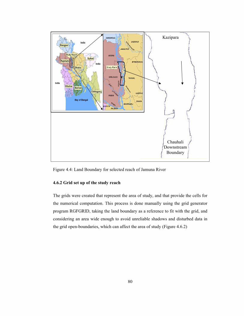
4.6 Model set-up 79
4.6.1 Land Boundaries 79
4.6.2 Grid set up of the study reach 80
4.6.3 Refine grid 81
4.6.4 Orthogonalise grid 82
4.6.5 Grid Smoothness (Aspect Ratio) 83
4.6.6 Bathymetry development 84
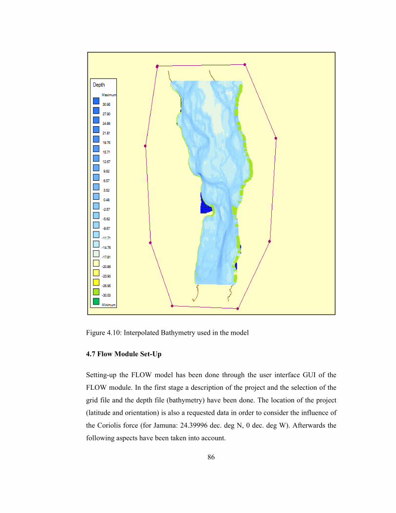
4.7 Flow module set-up 86
4.7.1 Dry Points and Thin Dams 87
4.7.2 Time Frame 87
4.7.3 Boundary set up 88
4.7.4 Initial conditions 91
Page 9
ix
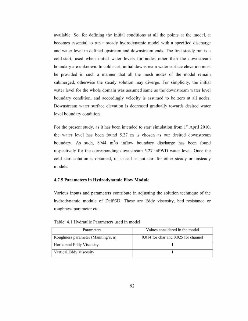
4.7.5 Parameters in hydrodynamic module 92
4.7.6 Morphological updating 93
4.7.7 Morphological “Switch" 94
4.7.8 Monitoring option 94
4.8 Summary 96
Chapter 5. Results and Discussions
5.1 General 97
5.2 Model calibration 98
5.2.1 Necessity of model calibration 98
5.2.2 Calibration data 99
5.3 Model verification 100
5.3.1 Necessity of model verification 100
5.3.2 Verification data 100
5.4 Simulation of the model 101
5.4.1 Comparison of observed and simulated bed elevations 102
5.4.2 Variation in velocity and sediment transport 106
5.4.3 Comparison of the simulated bathymetry in
September 2011 by Mike21 and Delft 125
5.5 Sensivity Analysis 126
5.5.1 Bottom roughness 128
5.5.2 Eddy Viscosity 128
Page 10
x
5.6 Summary 128
Chapter 6. Conclusions and Recommendations
6.1 General 130
6.2 Conclusions 130
6.3 Recommendations for further Study 131
References 133
Appendix A 139
Page 11
xi
List of Figures
Figure No. Page No.
Figure 1.1 River Systems of Bangladesh 4
Figure 1.2 Longitudinal profile of the Brahmaputra River 6
Figure 1.3 Brahmaputra-Jamuna River System within
Bangladesh Territory
9
Figure 1.4 Catchment Area of Major Rivers 10
Figure 2.1 Channel patterns 20
Figure 2.2 Various features of channels 21
Figure 2.3 Development of the Bengal Delta 29
Figure 2.4 Low-stage plan forms of the Jamuna River 32
Figure 2.5 Movement of the main channel for the period 1973-
1995 and planform in 1995
33
Figure 2.6 Relation between the elevation and the age of the land
along the Jamuna River
34
Figure 2.7 Plan forms of low flow, bar full, dominant and
minimum bank full as defined by FAP1 and FAP24
for the Jamuna River at the beginning of 1994
35
Figure 3.1 Mass fluxes entering and leaving an element 49
Figure 3.2 Surface stresses on a fluid element in 2 dimensions 51
Figure 3.3 Schematization of flux on the kmx layer 56
Figure 3.4. Schematic overview Delft3D calculation steps 62
Figure 3.5 Study Area on the Jamuna River 64
Figure 3.6 Water level gauge on the River Jamuna 67
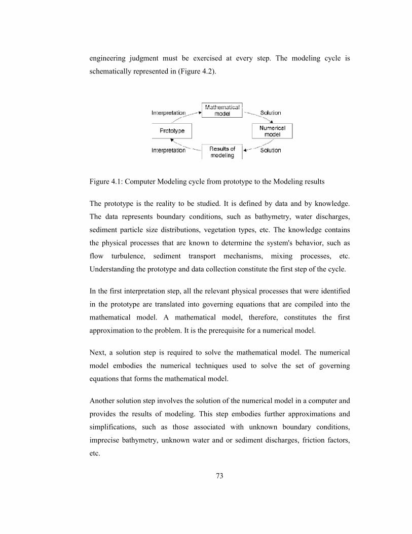
Figure 4.1 Computer Modelling cycle from prototype to the
Modeling results
73
Figure 4.2 Interaction among the main Delft3D modules 75
Figure 4.3 Structure of Delft3D 77
Figure 4.4 Land Boundary for selected reach of Jamuna River 80
Figure 4.5 Flow grids for selected reach of Jamuna River 81
Page 12
xii
Figure 4.6 Grids Refinement for selected reach of Jamuna River 82
Figure 4.7 Orthogonality of grids for selected reach of Jamuna
River
83
Figure 4.8 Aspect ratio of grids for selected reach of Jamuna
River
84
Figure 4.9 Measured bathymetry used in the model 85
Figure 4.10 Interpolated bathymetry used in the model 86
Figure 4.11 Courant number variation as function of the grid size 88
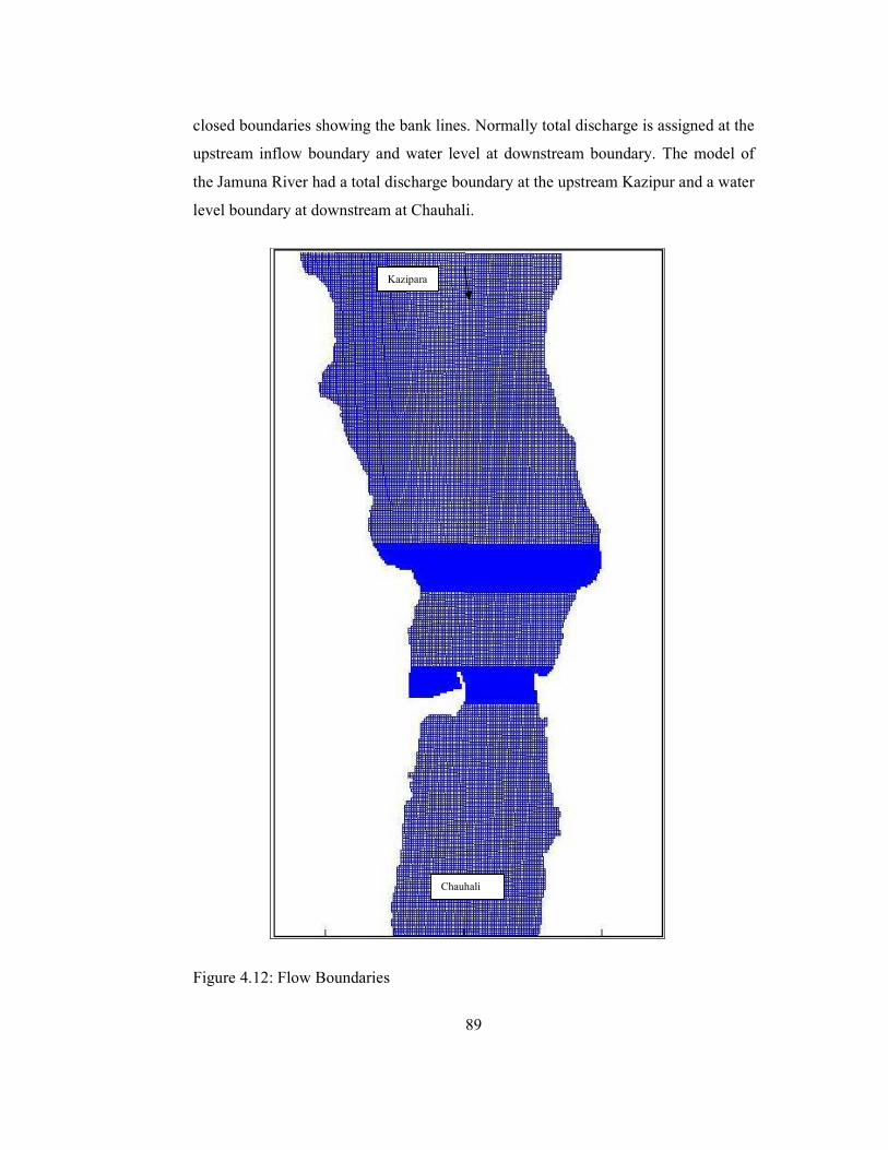
Figure 4.12 Flow Boundaries 86
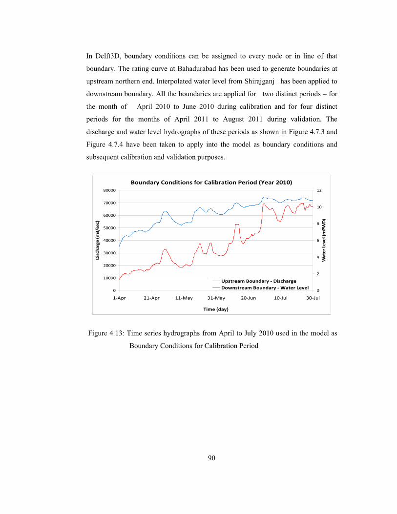
Figure 4.13 Time series hydrographs from April to July 2010 used
in the model as Boundary conditions for calibration
period
90
Figure 4.14 Time series hydrographs from April to October 2011
used in the model as Boundary Conditions for
Validation Period
91
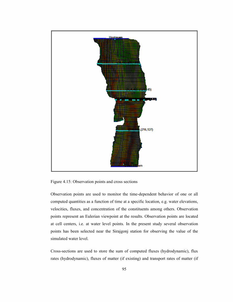
Figure 4.15 Observation points and cross sections 95
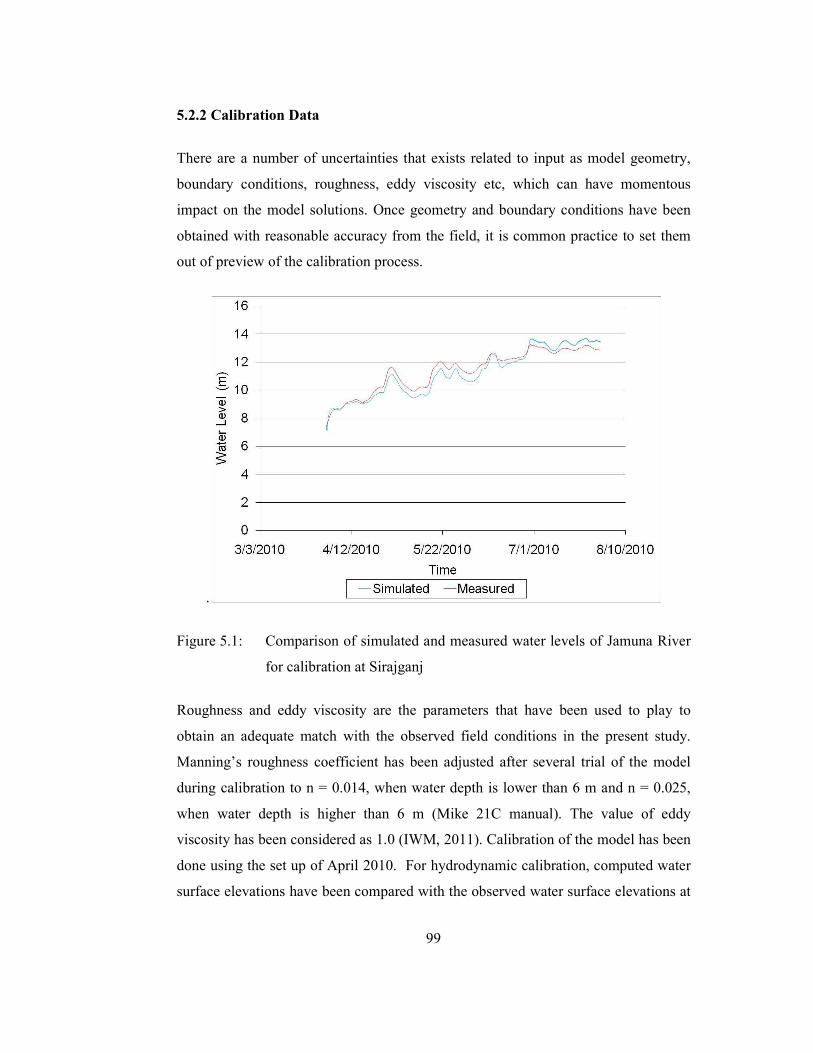
Figure 5.1 Comparison of simulated and measured water levels
of Jamuna River for calibration at Sirajganj
99
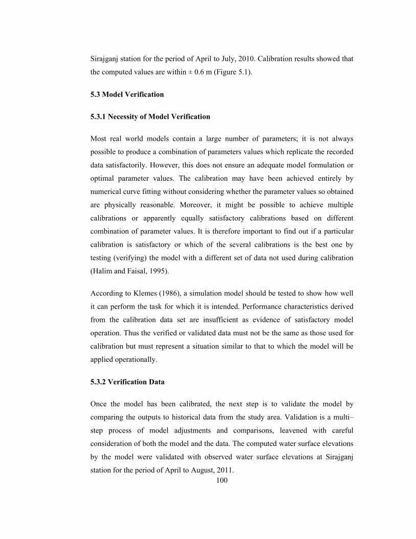
Figure 5.2 Comparison of simulated and measured water levels
of Jamuna River for validation at Sirajganj
101
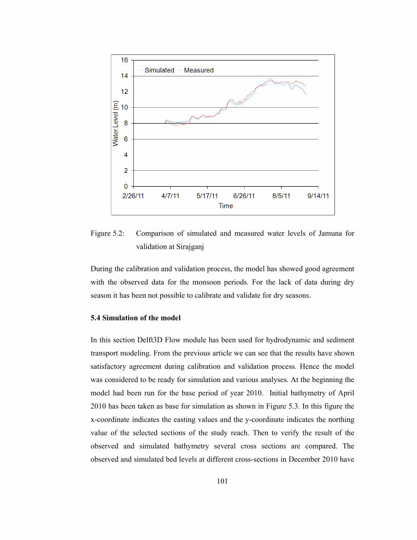
Figure 5.3 Cross Sections shown in Bathymetry of selected reach
of the Jamuna River for comparison
102
Figure 5.4 Comparison of Cross-Section at (Sec a-a) 103
Figure 5.5 Comparison of Cross-Section at (Sec b-b) 103
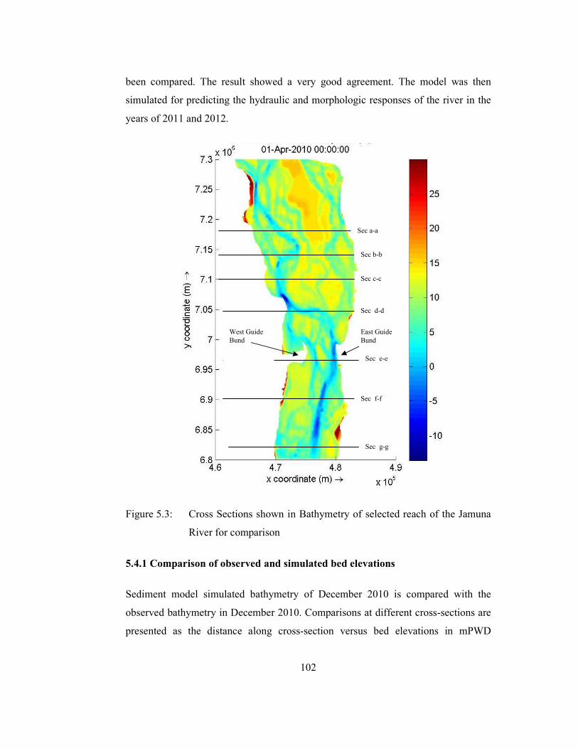
Figure 5.6 Comparison of Cross-Section at (Sec c-c) 104
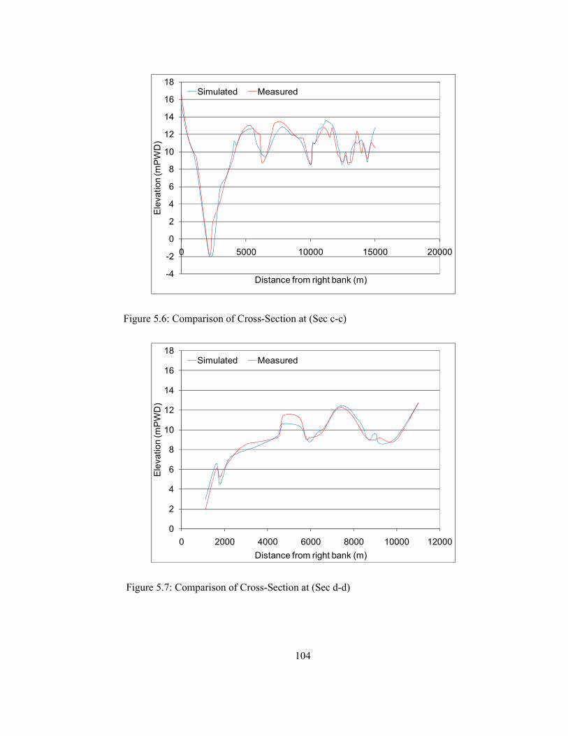
Figure 5.7 Comparison of Cross-Section at (Sec d-d) 104
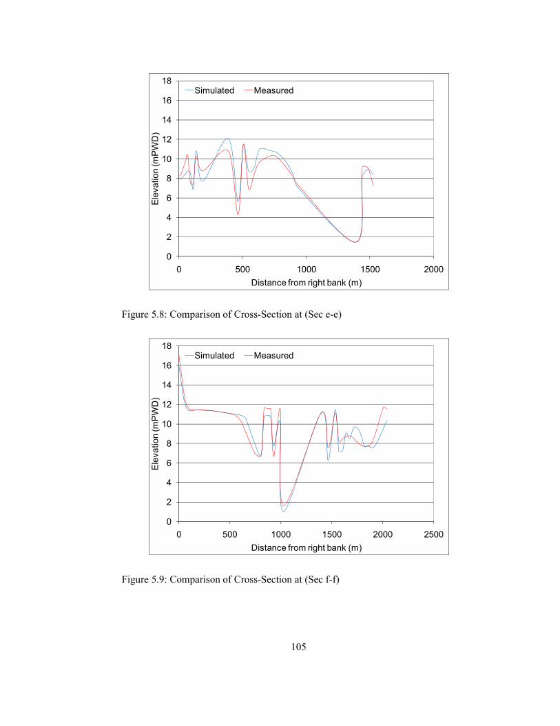
Figure 5.8 Comparison of Cross-Section at (Sec e-e) 105
Figure 5.9 Comparison of Cross-Section at (Sec f-f) 105
Figure 5.10 Comparison of Cross-Section at (Sec g-g) 106
Figure 5.11 Depth Averaged Velocity in 29/7/2010 108
Figure 5.12 Total Sediment Transport in 29/7/2010 108
Page 13
xiii
Figure 5.13 Depth Averaged Velocity in 27/1/2011 109
Figure 5.14 Total Sediment Transport in 27/1/2011 109
Figure 5.15 Depth Averaged Velocity in 27/7/2011 110
Figure 5.16 Total Sediment Transport in 27/7/2011 110
Figure 5.17 Depth Averaged Velocity in 25/1/2012 111
Figure 5.18 Total Sediment Transport in 25/1/2012 111
Figure 5.19 Depth Averaged Velocity in 24/7/2012 112
Figure 5.20 Total Sediment Transport in 24/7/2012 112
Figure 5.21 Bathymetry of selected reach of the Jamuna River in
April 2010
114
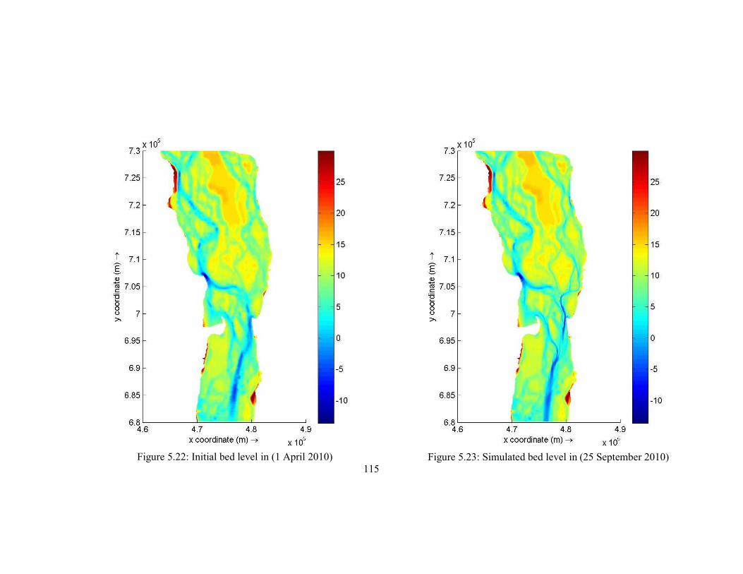
Figure 5.22 Initial bed level in (1 April 2010) 115
Figure 5.23 Simulated bed level in (25 September 2010) 115
Figure 5.24 Simulated bed level in (23 September 2011) 116
Figure 5.25 Simulated bed level in (28 September 2012) 116
Figure 5.26 Cross-section at Section 1 117
Figure 5.27 Cross-section at Section 2 119
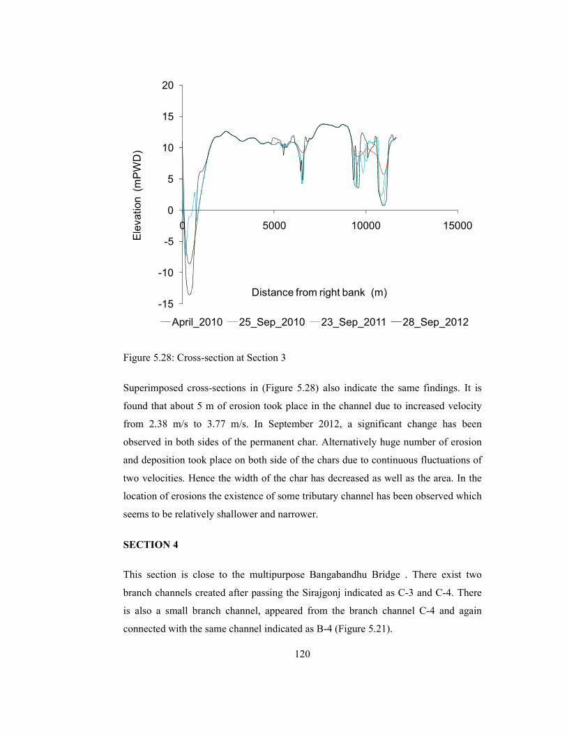
Figure 5.28 Cross-section at Section 3 120
Figure 5.29 Cross-section at Section 4 121
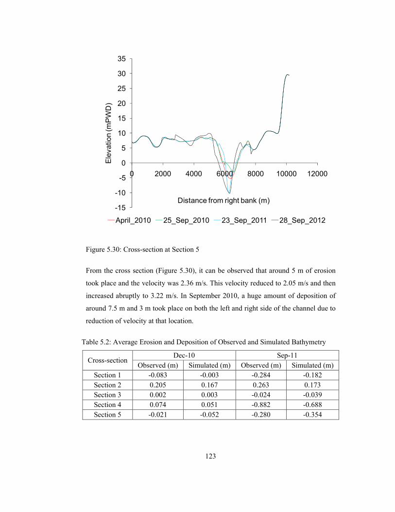
Figure 5.30 Cross-section at Section 5 123
Figure 5.31 Simulated bathymetry by Mike 21 (September 2011) 125
Figure 5.32 Simulated bathymetry by Delft 3D (September 2011) 125
Figure 5.33 Influence of Manning parameter on amplitudes of
water level
127
Figure 5.32 Influence of Eddy viscosity on amplitudes of water
level
128
Page 14
xiv
List of Tables
Table No. Page No.
Table 1.1 Losses of livelihoods 12
Table 1.2 Losses of cultivated land 12
Table 2.1 Grain size (mm) of bed material collected in 1993-
1994 by FAP24 (1996)
27
Table 4.1 Hydraulic parameters used in model 92
Table 5.1 Average sediment transport rate of the river for
various seasons
113
Table 5.2 Average erosion and deposition of observed and
simulated bathymetry
123
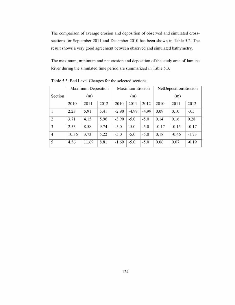
Table 5.3 Bed level changes for the selected sections 124
Table A.1 Observed and simulated water level data for
calibration
139
Table A.2 Observed and simulated water level data for
validation
140
Page 15
xv
Acknowledgements
I express my deepest thanks and appreciation to my superviser Dr. Umme Kulsum
Navera, Professor and Head, Department of Water Resources Engineering, BUET for
her constant supervision, valuable guidance and unlimited encouragement during the
period of research work. It was a great opportunity for me to work with Prof. Dr.
Umme Kulsum Navera, whose unfailing eagerness made the study a success.
Sincere thanks also goes to the Members of the Examination Committee, Dr. M.A.
Matin, Professor, Department of Water Resources Engineering, BUET; Dr. Md.
Sabbir Mostafa Khan, Professor and Head of WRE Department, BUET and Mr. Abu
Saleh Khan, Deputy Executive Director of Institute of Water Modelling, for their
special interest, valuable comments and suggestions regarding the study.
I am indebted to all the officials of the River Engineering Division, IWM, Dhaka and
to the officials of River Hydrology and Research Circle, BWDB, Dhaka for their
help and cooperation in collecting the required data and information.
I would also like to express my gratitude to my parents and my husband for their
sincere support, sacrifice, inspiration and help during the entire period of this study.
Finally I am grateful to almighty Allah.
Page 16
xvi
Abstract
Simulation of sediment transport rate at the river Jamuna and variation of bed level
along the river is carried out by using a two dimensional morphological model. Non-
cohesive sediment transport module of Delft 3D Flow is used for the simulation. The
upstream boundary of the model is taken at 30 Km upstream of Bangabandhu
Bridge and downstream boundary is taken at 20 Km downstream of Bangabandhu
Bridge.
Simulation period is taken from April 2010 to December 2012. Simulation is carried
out for hydrodynamic calibration and for sediment transport rates. The cross-sections
are taken at the locations which are vulnerable, such as Subaghacha, Sirajganj,
Jamuna Bridge and also in the upstream near Kazipur and downstream near Chauhali
etc. In the Morphology tab, the morphological scale factor has been set to 8.25 which
extend the 121 days hydrodynamics to about 1000 days of morphological change.
Calibration and validation are carried out against field observations (water level) of
2010 and 2011 respectively. Comparisons between simulated and observed water
level are taken at the Sirajgonj station. The results showed satisfactory agreement
with observed values.
For hydrodynamic and morphological computation, a time series discharge data is
used at the upstream boundary and water level data as downstream boundary.
Observed and simulated bed level elevation of 2010 has been compared and the
comparison showed a very good agreement. After calibration of the model, the net
amount of erosion and deposition along the river reach is computed. Finally, cross-
sectional variation of bottom level during the monsoon seasons from 2010 to 2012
has been observed.
Results reveal that erosion takes place in the channel bed and the deposition mainly
takes place to the adjacent char areas and increased its width and area. It is also
evident that the channel has been shifted westwards of the reach due to shifting of the
bank line of the river. Many tributary and distributaries have been appeared due to
progressive erosion. In Sirajgonj, the sediment transport capacity seems to be the
Page 17
xvii
highest due to higher velocity of flow. The zones of higher velocity has higher
sediment transport capacities therefore occurs more erosion
Page 18
1
CHAPTER 1
INTRODUCTION
1.1 General
Bangladesh is a riverine country with hundreds of rivers overlaying its landscape.
Because of its inherent alluvium nature, the rivers of Bangladesh are
morphologically dynamic characterized by erosion and sedimentation, which results
in changes in hydraulic geometry; plan form and longitudinal profile of the rivers
(Habibullah, 1987). Aggradations, degradation or change in plan forms; change in
river bed and meandering characteristics are most common features in the rivers of
Bangladesh, affecting the major rivers as well as the medium and the minor rivers.
When bank erosion of a river takes place the drainage capacity of the river and
navigation is hampered and consequently a large number of populations are directly
or indirectly affected. A simple solution could be through local protective measures
for the time being but properly designed river control and training structures are
required to reduce the loss of lands. Before intervening with the natural behavior of a
river, the consequences in both the near future and the long run should be considered.
Each river style is characterized by a distinctive set of attributes, analyzed in terms of
channel plan form, the geomorphic units that make up a reach, and bed material
texture. The identification and interpretation of geomorphic units allows
interpretation of processes that reflect the range of behavior of a river style. Thus
helps in understanding of the behavior of the river in natural and disturbed conditions
in an effective manner.
Bangladesh is a country blessed with abundant natural source of fresh sweet water.
The three major rivers originating from Himalayas (Indus, Ganges and Brahmaputra)
and flowing down the Northern regions of Indian Sub-continent reaches the Bay of
Bengal through Bangladesh (Rahman et al., 2007). These rivers frequently flood the
vast plain of Bangladesh, deposit silt and contributed largely to create the fertile soil.
People of this land use the water from these rivers and their tributaries for cultivation
and livelihood. For thousands of years, people settled in this fertile and easily
Page 19
2
cultivable land along the rivers. There are 405 rivers in total, Brahmaputra, Padma,
Meghna, Jamuna, Karnafuli are the bigger rivers among all. Total length of rivers is
24,140 Km. In an average yearly 844,000 million cubic meters of water flows into
the country, the sediment load that comes along the flow is more than a billion ton
(Imran, 2011).
The profusion of rivers can be divided into five major networks. The Jamuna
originates as the Yarlung Tsangpo River in China's Xizang Autonomous Region
(Tibet) and flowing through India's state of Arunachal Pradesh, where it becomes
known as the Brahmaputra ("Son of Brahma"). There it turns to south into Asam. In
flood plain of Asam, it flows towards west and then again veers into south and then
enters Bangladesh through Kurigram district (at the border of Kurigram Sadar and
Ulipur upazilas). Presently the Brahmaputra continues southeast from Bahadurabad
(Dewanganj upazila of Jamalpur district) as the Old Brahmaputra and the river
between Bahadurabad and Aricha is the Jamuna, not Brahmaputra. The Hydrology
Directorate of the Bangladesh Water Development Board (BWDB) refers to the
whole stretch as the Brahmaputra-Jamuna. Tista, Dudhkumar, Korotoa-Atrai,
Hurasagar etc. are the main tributaries of Jamuna River.
The total length of the Tsangpo-Brahmaputra-Jamuna River up to its confluence with
the Ganges is about 2,700 km. Within Bangladesh territory, Brahmaputra-Jamuna is
276 km long, of which Jamuna is 205 km. It receives waters from five major
tributaries that total some 740 kilometers in length.
The second system is the Padma-Ganges originated in the Gangotri Glacier of the
Himalaya, the Ganges runs through Himachal Pradesh, Uttar Pradesh, Bihar and
West Bengal in India. For some 110 km the Ganges River forms the western
boundary between India and Bangladesh before it enters Bangladesh at Durlavpur
Union in Shibganj Upazila in the district of Chapai Nababganj to the Bay of Bengal.
Just west of Shibganj, the distributary Bhagirathi emerges and flows southwards as
the Hooghly. After the point where the Bhagirathi branches off, the Ganges is
officially referred to as the Padma.
Page 20
3
Further downstream, in Goalando, 2200 km away from the source, the Padma is
joined by the mighty Jamuna (Lower Brahmaputra) and the resulting combination
flows with the name Padma further east, to Chandpur. Here, the widest river in
Bangladesh, the Meghna, joins the Padma, continuing as the Meghna almost in a
straight line to the south, ending in the Bay of Bengal.Its main tributary is the
Mahananda; its principal distributary is the Madhumati (called the Garai in its upper
course) at right bank and Ichamati, Boral, Badai, Khalshadingi at left bank.
The third network is the Surma-Meghna River System. Surma River rises in the
Manipur Hills in northern Manipur state, India, where it is called the Barak, and
flows west and then southwest into Mizoram state. There it veers north into Assam
state and flows west past the town of Silchar. At the border with Bangladesh, where
the river divides, the north-eastern branch is called the Surma River and the south-
eastern the Kushiyara River. The Surma is also known as the Baulai River after it is
joined by the Someswari River at Sukhair Rajapur Union in Dharmapasha Upazila in
Sunamganj District. When the Surma and the Kushiyara rejoin above Bhairab Bazar,
the river is known as the Meghna River, which flows south past Dhaka and enters the
lower Padma River. Near Muladhuli in Barisal district, the Safipur River is an
offshoot of the Surma. At Sarail of Brahmanbaria District, the river Titas emerges
from Meghna and after circling two large bends by 240 km, falls into the Meghna
again near Nabinagar Upazila. Titas forms as a single stream but braids into two
distinct streams which remain separate before re-joining the Meghna.
In Daudkandi, Comilla, Meghna is joined by the great river Gomoti, created by the
combination of many streams. The Dakatia River is also part of this river in Comilla
district.(BWDB, 2011)
Barak River flows separately to North-eastern as Surma River and to South-Eastern
at Jakiganj Upazila in Sylhet District, originating from the hilly regions of eastern
India. The Meghna is formed inside Bangladesh by the joining of the Surma and
Kushiyara rivers at Bajitpur in Keshoreganj. Down to Matlab in Chandpur, Meghna
joins with Padma River and is hydrographically referred to as the Upper Meghna.
Page 21
4
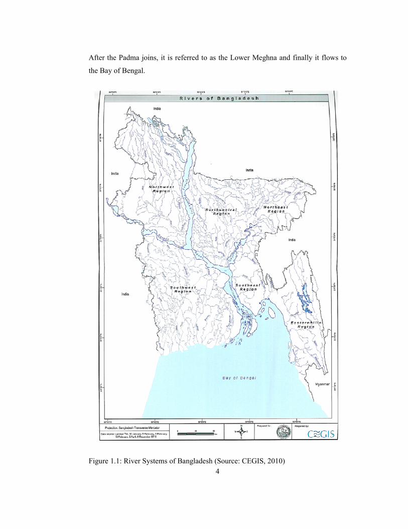
After the Padma joins, it is referred to as the Lower Meghna and finally it flows to
the Bay of Bengal.
Figure 1.1: River Systems of Bangladesh (Source: CEGIS, 2010)
Page 22
5
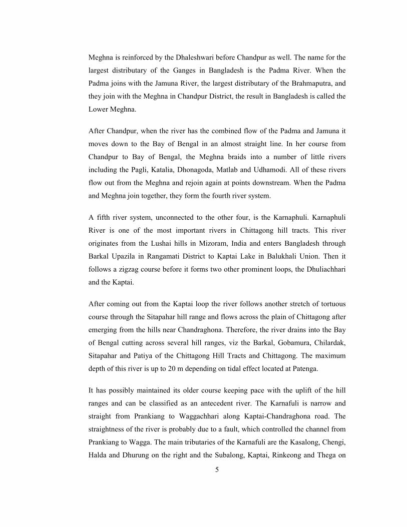
Meghna is reinforced by the Dhaleshwari before Chandpur as well. The name for the
largest distributary of the Ganges in Bangladesh is the Padma River. When the
Padma joins with the Jamuna River, the largest distributary of the Brahmaputra, and
they join with the Meghna in Chandpur District, the result in Bangladesh is called the
Lower Meghna.
After Chandpur, when the river has the combined flow of the Padma and Jamuna it
moves down to the Bay of Bengal in an almost straight line. In her course from
Chandpur to Bay of Bengal, the Meghna braids into a number of little rivers
including the Pagli, Katalia, Dhonagoda, Matlab and Udhamodi. All of these rivers
flow out from the Meghna and rejoin again at points downstream. When the Padma
and Meghna join together, they form the fourth river system.
A fifth river system, unconnected to the other four, is the Karnaphuli. Karnaphuli
River is one of the most important rivers in Chittagong hill tracts. This river
originates from the Lushai hills in Mizoram, India and enters Bangladesh through
Barkal Upazila in Rangamati District to Kaptai Lake in Balukhali Union. Then it
follows a zigzag course before it forms two other prominent loops, the Dhuliachhari
and the Kaptai.
After coming out from the Kaptai loop the river follows another stretch of tortuous
course through the Sitapahar hill range and flows across the plain of Chittagong after
emerging from the hills near Chandraghona. Therefore, the river drains into the Bay
of Bengal cutting across several hill ranges, viz the Barkal, Gobamura, Chilardak,
Sitapahar and Patiya of the Chittagong Hill Tracts and Chittagong. The maximum
depth of this river is up to 20 m depending on tidal effect located at Patenga.
It has possibly maintained its older course keeping pace with the uplift of the hill
ranges and can be classified as an antecedent river. The Karnafuli is narrow and
straight from Prankiang to Waggachhari along Kaptai-Chandraghona road. The
straightness of the river is probably due to a fault, which controlled the channel from
Prankiang to Wagga. The main tributaries of the Karnafuli are the Kasalong, Chengi,
Halda and Dhurung on the right and the Subalong, Kaptai, Rinkeong and Thega on
Page 23
6
the left. Flowing to the west through Rangunia Upazila and then keeping Raozan
Upazila on the north and Boalkhali Upazila on the south, it receives the waters of the
Halda River at Kalurghat just above the railway bridge. It then turns south, receives
the waters of the Boalkhali and other khals and turns west circling round the eastern
and southern sides of Chittagong Town. From the extreme corner of the Chittagong
Port to the west, it moves southwest to fall into the Bay of Bengal 16.89 km below.
The river meets Padma River in Chandpur District. Major tributaries of the Meghna
include the Dhaleshwari River, Gumti River, and Feni River. The Meghna empties
into the Bay of Bengal via four principal mouths, named Tetulia, Shahbazpur, Hatia,
and Bamni.
1.2 Origin of Jamuna River
The Brahmaputra, also called Tsangpo-Brahmaputra is a transboundary river and one
of the major rivers of Asia. The 3000 km long river springs in the western part of the
Tibet Autonomous Region [Xizang] of China not far from the sources of the Ganges
River and Indus River (Figure 1.2).
Figure 1.2: Longitudinal profile of the Brahmaputra River (Source: Zhang, 1998)
It springs at an altitude of 5100 m from the Chemayungdung glacier near mount
Kailas in the Himalayas. It flows for about 1400 km in an easterly direction across
Page 24
7
the Tibetan plateau, which is bordered by the Himalayas in the south and the Gandise
Mountains in the north, while it descends to 3000 m. In this reach the river is known
as the Tsang Po or Yarlung Zangbo (Jiang) River. Not far from Nyingchi at mount
Namche Barwa the river enters one of the world’s largest canyons; meanwhile
rapidly descending. At an altitude of 200 m above sea level it leaves the Himalayan
range as the Dihang River. The canyon is the main access route for the moist air
currents from the Indian Ocean as a result of which the annual average precipitation
varies on the Tibetan plateau from 200 mm at the western end to 900 mm at the
eastern end. It was not before 1880 that the connection between the Yarlung Zangbo
and the Brahmaputra was finally confirmed by the exploration of Pandit Kishen
Singh (Montgomerie, 1885) and still, its narrow canyon through the eastern part of
the Himalayas remains one of world’s least explored regions (Bian, 1998; National
Geographic, 1999).
The Dihang River joins with the Lohit River and Dibang River at west of the town of
Sadiya in the Indian province Assam, after which it flows west through the plains of
the Indian province Assam as the Brahmaputra River.
As the Brahmaputra River reaches the ninety degrees east meridian it makes a sharp
left turn, goes south and enters Bangladesh with the name of Jamuna. The total
length of the river from its source in southwestern Tibet to the mouth in the Bay of
Bengal is about 2,850 km (including Padma and Meghna up to the mouth). The
Jamuna enters Bangladesh east of Bhabanipur (India) and northeast of Kurigram
district. Originally, the Jamuna (Brahmaputra) flowed southeast across Mymensing
district where it received the Surma River and united with the Meghna, as shown in
Rennell’s Atlas (1785). By the beginning of the 19th century its bed had risen due to
tectonic movement of the Madhupur Tract and it found an outlet farther west along
its present course. It has four major tributaries: the Dudhkumar, Dharla, Teesta and
the Baral-Gumani-Hurasagar system. The first three rivers are flashy in nature, rising
from the steep catchment on the southern side of the Himalayas. The main
distributaries of the Jamuna River are the Old Brahmaputra River, which leaves the
Page 25
8
left bank of the Brahmaputra River 20 km north of Bahadurabad, and the New
Dhaleswari River just south of the Bangabandhu Bridge (Figure 1.3).
The combined delta of Brahmaputra River and Ganges River (59,000 km2) is twice
as large as the second largest delta in the world (the one of the Niger River). Their
combined average discharge (32,000 m3/s) ranks third after the Congo River and the
Amazon River, while the combined drainage area of the Ganges River (1,100,000
km2) and Brahmaputra River (924,000 km
2) ranks only ninth. The river serves as an
important inland waterway on both the Tibetan plateau and the Indian and
Bangladeshi plains.
Page 26
9
Figure 1.3: Brahmaputra-Jamuna River System within Bangladesh Territory
(Source: Banglapedia, 2010)
Page 27
10
Catchment Characteristics
The Brahmaputra-Jamuna drains the northern and eastern slopes of the Himalayas,
and has a catchment area of 5, 83,000 sq.km. 50.5 percent of which lie in China, 33.6
percent in India, 8.1 percent in Bangladesh and 7.8 percent in Bhutan. The catchment
area of Jamuna River in Bangladesh is about 47,000 sq. km. The average annual
discharge is about 19,200 m3/sec, which is nearly twice that of the Ganges. The
Brahmaputra River is characterized by high intensity flood flows during the monsoon
season, June through September. There is considerable variation in the spatio-
temporal distribution of rainfall with marked seasonality.
Figure 1.4: Catchment Area of Major Rivers (Source: CEGIS, 2011)
Precipitation varies from as low as 120 cm in parts of Nagaland to above 600 cm in
the southern slopes of the Himalayas. In Bangladesh territory rainfall varies from 280
cm at Kurigram to 180 cm at Ganges-Brahmaputra confluence (FAP2). Monsoon
rains from June to September accounts for 60-70% of the annual rainfall. These rains
that contribute a large portion of the runoff in the Brahmaputra and its tributaries are
primarily controlled by the position of a belt of depressions called the monsoon
trough extending from northwest India to the head of the Bay of Bengal.
Page 28
11
Deforestation in the Jamuna watershed has resulted in increased siltation levels, flash
floods, and soil erosion. Occasionally, massive flooding causes huge losses to crops,
life and property. Periodic flooding is a natural phenomenon which is ecologically
important because it helps maintain the lowland grasslands and associated wildlife.
Periodic floods also deposit fresh alluvium replenishing the fertile soil of the Jamuna
River Valley. (Ref: IWM, Monitoring of Hydraulic and Morphological conditions of
Jamuna River for the safety of Bangabandhu Bridge).
1.3 Background of the study
The Jamuna River in Bangladesh is a braided sand-bed river characterised by
substantial planform changes during individual floods. The Jamuna is a braided
stream characterised by a network of interlacing channels with numerous sandbars
enclosed in between them. The sandbars, known in the Bengali as chars do not,
however, occupy a permanent position. The river deposits them in one year very
often to destroy and redeposit them in the next rainy season. The average discharge
during flood amounts is about 60,000 m3/s, which combined with the flooding
caused by the other large rivers, results in an inundation of 20–30% of the country.
However, in 1987 and 1988 extreme floods occurred which led to the flooding of
40% and 60% of the country, respectively (Thorne and Russel, 1993). The peak
discharge of 1988 flood was more than 90,000 m3/s and it coincided with the flood
peak of the Ganges River (Thorne et al., 1993). These floods cause more damage to
property of individuals, to infrastructural works, and to society as a whole, thereby
retarding (or even stopping) the socio-economic development of the rural areas.
For this reason a number of internationally funded projects - jointly known as the
Flood Action Plan (FAP) for Bangladesh - were started in 1990/1991 to investigate
the problems associated with the flooding and to find ways to solve them.
Erosion of river bank in the Jamuna River is one of the major problems in
Bangladesh. Thousands of people become homeless every year and they lose their
homestead and croplands. Mosques, schools, hospitals and other infrastructures are
Page 29
12
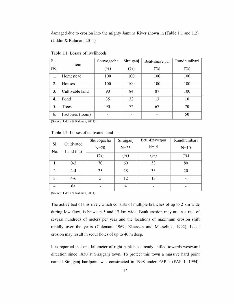
damaged due to erosion into the mighty Jamuna River shown in (Table 1.1 and 1.2).
(Uddin & Rahman, 2011)
Table 1.1: Losses of livelihoods
Sl.
No. Item
Shuvogacha
(%)
Sirajganj
(%)
Betil-Enayetpur
(%)
Randhunibari
(%)
1. Homestead 100 100 100 100
2. Houses 100 100 100 100
3. Cultivable land 90 84 87 100
4. Pond 35 32 13 10
5. Trees 90 72 67 70
6. Factories (loom) - - - 50
(Source: Uddin & Rahman, 2011)
Table 1.2: Losses of cultivated land
Sl.
No.
Cultivated
Land (ha)
Shuvogacha
N=20
Sirajganj
N=25
Betil-Enayetpur
N=15
Randhunibari
N=10
(%) (%) (%) (%)
1. 0-2 70 60 53 80
2. 2-4 25 28 33 20
3. 4-6 5 12 13 -
4. 6> - 4 - -
(Source: Uddin & Rahman, 2011)
The active bed of this river, which consists of multiple branches of up to 2 km wide
during low flow, is between 5 and 17 km wide. Bank erosion may attain a rate of
several hundreds of meters per year and the locations of maximum erosion shift
rapidly over the years (Coleman, 1969; Klaassen and Masselink, 1992). Local
erosion may result in scour holes of up to 40 m deep.
It is reported that one kilometer of right bank has already shifted towards westward
direction since 1830 at Sirajganj town. To protect this town a massive hard point
named Sirajganj hardpoint was constructed in 1998 under FAP 1 (FAP 1, 1994).
Page 30
13
Without this hard point Sirajganj town would be washed out several years back. As
Hard point is a local erosion-resistant feature constructed on a river bank or
projecting out into the river. So, this hard point plays a vital role for the existence of
Sirajganj town. Erosion is being continued just upstream of the Sirajganj town due to
morphological change. Shuvogacha under Kazipur Upazila of Sirajganj district is one
of the erosion prone areas along the right bank of the Jamuna River.
The morphology of Jamuna River is affected by the construction of one of the
national assets of Bangladesh, the Bangabandhu Bridge with river training works as a
part of bridge construction in 1998 on Jamuna River. Number of river training works
(guide bunds and hard points) was constructed in addition with this 4.8km long road
bridge, by constricting the river width from 10 km to 4.8 km. This Bridge connects
Bhuapur on the Jamuna River’s east bank to Sirajganj on its west bank (IWM, 2011).
The river training works include two guide bunds, one on each side of the river. The
guide bunds supplement the hard points at Sirajganj and Bhuapur. The intensity of
channel shifting has been increased due to regulation of river width at Sirajganj–
Bhuiyapur section from 11 km to 4.8 km. Planform analysis shows that the major
channel has been stressed to migrate (315 m/year) eastwards. The Jamuna River is
adjusted to a new morphology after construction of the Bangabandhu Bridge. A big
permanent char is formed downstream of the Bangabandhu Bridge. But a branch
channel is flowing in between bank line and the char. A lot of erosion affected
people living near the bank line and on the adjacent char (Uddin and Rahman, 2011).
Efficient and potentially affordable solutions to the problem of bank erosion have
been developed and tested under the FAP (Flood Action Plan) 21/22 “Bank
Protection and River Training/ Active Flood Plain Management (AFMP) Pilot
Project”. The FAP 21 component dealt with structures to stabilize banks, where as
FAP 22 component dealt more generally with measures and strategies to train the
river channels and, at the same time, to increase or to maintain the hydraulic
efficiency of the river in transporting water and sediments in combination with an
optimum use of the flood plains (Rahman and Osman, 2009). For this purpose some
test structures (groynes and revetments) were designed and constructed along the
braided Jamuna River, and their performance was monitored.
Page 31
14
Considering the dynamic situations prevail in the Jamuna River a Morphodynamic
study has an utmost necessity to identify the morphological changes of the river.
1.4 Scope of mathematical modeling
River sedimentation and morphological processes are among the most complex and
least understood phenomena in nature. Due to the fact that they intimately affect on
our living conditions, scientists and engineers have been looking for better tools to
improve our understanding and enhance the quality of our lives ever since the
beginning of human civilization. In early times, the research methodologies were
primarily based on field observation and physical modeling. However, it is neither
practical, nor possible to measure all river processes continuously and
simultaneously. Field data represents very closely the physical reality of the existing
processes in the river. Whatever the detail and frequency of surveys, the
representation will always be discrete in space and time, especially during the
monsoon period when the rate of change of bed level is high; the bathymetry would
in general not be expected to be in equilibrium with local flow conditions. In this
case measurement of, say, sediment concentrations at certain location would depend
of course on local flow conditions, but also on conditions upstream and on the flow
history. Field surveys with the purpose of understanding the process would then
include very large amount of information. To collect the data and analyze it would be
a very costly and time-consuming task. In that respect mathematical modeling is an
alternate tool to understanding the detail physical processes in the nature.
Mathematical modeling has been introduced as a tool to interpret the information
provided by the field data in an integrated way. The mathematical models enable
interpolation and extrapolation in space and time based on the observations from the
field and on the understanding of the physical processes and their interaction to the
extent that this has been incorporated in the model. (Ali, 2004)
Various 1-D, 2-D and 3-D hydrodynamic and sediment modules are in use in water
engineering sector. Some of the widely used models are briefly summarized:
Page 32
15
HEC model Series, including HEC-UNET, HEC-6, and HEC-RAS, is a set of one-
dimensional models of river hydrodynamics and sediment transport provided by the
U.S. Army Corps of Engineers.
MIKE model series together comprises a very extensive set of finite difference
models in one-, two- and three dimensions. Most of the MIKE models (MIKE-11,
MIKE-12, and MIKE-3) use a rectangular, potentially nested, grid. Modules exist to
cover hydrodynamics, sediment transport, water quality, and wave
generation/transformation. MIKE-21C is a newer one which uses curvilinear grid.
Finite element version (MIKE-FM) is also in ongoing processes.
CH2D/CH3D is two- and three-dimensional finite difference models of
hydrodynamics, salinity, and sediment transport. The models use a curvilinear
orthogonal grid. It can be used together with CE-QUAL-ICM to model water quality.
CH2D/CH3D are developed and maintained by the U.S. Army Corps of Engineers.
However, the software is not freely available to users outside the U.S. Army Corps of
Engineers. Model development and application are possible through a cooperative
agreement with the Waterways Experiment Station or other branches within the
Corps.
ADCIRC is a two- and three- dimensional finite element hydrodynamics model using
an irregular grid and provided by the U.S. Army Corps of Engineers. ADCIRC is
supported by the SMS preprocessing and display suite.
GEMSS consists of a three- dimensional finite difference hydrodynamic, water
quality, and sediment transport model, with a curvilinear orthogonal grid. The model
uses the same basic hydrodynamic model (GLLVHT) as CE-QUAL-W2. The model
is developed by J.D. Edinger Associates. Model development and application are
possible only through a cooperative agreement with the developers.
RMA model series, together with the SED-2D model, is a set of one-, two-, and
three-dimensional models of hydrodynamics, sediment transport and water quality.
The RMA models are finite element models. This model can be run with 1-D
Page 33
16
elements, has significant computational efficiency. It has the capability of addressing
certain control structures, but not all the structures envisioned for the ponds. The
models are in the public domain. RMA is supported by the SMS preprocessing and
display suite.
TELEMAC model series comprises a set of two- and three-dimensional finite
element models of hydrodynamics, with modeling of salinity provided by WQ-2D
and WQ-3D, and sediment transport by SUBIEF. The models use irregular triangular
grids. TELEMAC and the associated models are commercially available from H.R.
Wallingford, U.K.
SMS is a comprehensive environment for one-, two- and three-dimensional
hydrodynamic modeling. SMS is used as a pre- and post-processor for surface water
modeling, analysis and design. It includes tools for managing, editing and visualizing
geometric and hydraulic data and creating, editing and formatting mesh/grid for use
in numerical analysis.
SOBEK is a powerful modeling framework for flood forecasting, modeling of
drainage systems, control of irrigation systems, sewer overflow design, river
morphology, salt intrusion and surface water quality. The components within the
SOBEK modeling framework simulate the complex flows and the water related
processes in almost any system. The components represent phenomena and physical
processes in an accurate way in one dimensional (1D) network systems and on two
dimensional (2D) horizontal grids. It is the ideal tool for guiding the designer in
making optimum use of resources.
The Delft3D modeling system, developed by Delft Hydraulics (www.wldelft.nl), is
capable of simulating hydrodynamic processes due to waves, tides, rivers, winds and
coastal currents. Hydrodynamic flow is simulated with the FLOW module (WL Delft
Hydraulics, 2001), which solves the unsteady shallow water equations in two (depth-
averaged) or three dimensions. It has been applied to model conditions of flow,
sediment transport and morphological developments in the present study due to its
highly flexible tool for various applications. The Delft3D can be run in Cartesian
Page 34
17
(equidistant or stretched) or curvilinear coordinates; all necessary grid generation
software for creating curvilinear grids is included with the Delft3D package.
As mathematical models have their limitations, they cannot stands alone. Results
should be assessed critically against field/laboratory data to assure that misleading
conclusions are not drawn from a poorly designed and calibrated mathematical
model.
1.5 Objectives of the study
Based on the above study an attempt has been made to simulate the bed level
changes of the river Jamuna by using the hydrodynamic and morphological model.
The key features, to which this study limits itself, are as follows:
1. To apply Delft3D-flow, in order to carry out simulations of flows, sediment
transports, morphological developments for the selected reach of Jamuna
River.
2. To obtain the bed level changes of the selected reach of Jamuna River.
3. To calibrate and validate the model with the field observation data.
4. To compare the results with other model output.
The main outcome of the present study is to understand the hydrodynamic and
morphological changes of the selected reach of the Jamuna river with the aid of
Delft3D-FLOW hydrodynamic module where the sediment version of DELFT3D-
FLOW dynamically updates the elevation of the bed at each computational time-step.
The following processes will be simulated after several runs using two or more years
of consecutive hydrographs:
1. Erosion and deposition in main channels at the monsoon period of the year
2. Possible bed level changes with time
3. Sediment transport variation with respect to depth average velocity.
Page 35
18
1.6 Organization of the report
The first chapter of the study gives a brief presentation of the hydrodynamic and
morphological processes of the overall river system of Bangladesh. It emphasizes the
need of scope of mathematical modeling tools for analyzing the phenomenon and the
background of the present study. It also includes the objectives of the present study.
The second chapter contains a description of the available information sources that
have been used for this research, short account of previous studies and literature
available in the domain in question. Also a short description about the Jamuna river
of its course and features etc are also discussed.
The third chapter presents the basic theory and equations used to model the
hydrodynamic and morphological changes of the river and also the step by step
processes that have been done during this study means the methodology has been
presented shortly. The calibration and validation processes using different parameters
have been shown in this chapter.
The fourth chapter comprises a brief description of the models developed under this
study. The generation of grid, land boundaries, bathymetries and also the set-up of
Flow module is discussed briefly in this chapter.
The fifth chapter presents an analysis and interpretation of the output from the
mathematical modeling and its application to the engineering interventions. Mainly
the results include the comparison of the observed and simulated bed levels, analysis
of the selected river reach, sediment transport rate at various periods of the year etc.
Also the sensitivity analysis of the model has been included in this chapter.
Finally the study ends in chapter six by drawing conclusion and recommendation for
the future study. This chapter contains a summary of the overall results of this
research, including comments about the modeling process, and gives
recommendations for the control and improvement of the conditions in Jamuna
River, and to recover the sediment transport balance in the area so as to control the
erosion/accretion problem.
Page 36
19
CHAPTER 2
LITERATURE REVIEW
2.1 General
The mighty rivers, the Ganges, the Jamuna and the Meghna and their distributaries
and tributaries flowing through Bangladesh are heavily charged with sediment and
major part of Bangladesh is formed from sediment deposited by them. The erosion
and deposition have complicated variations over time and space due to the abrupt
changes of flow and sedimentation.
The Brahmaputra, one of the largest braided rivers in the world, originates from the
Himalayas and enters Bangladesh at Kurigram as Jamuna. Though the history of
Jamuna is not more than 250 years, it shows very severe changes in its course due to
anthropogenic influences. Various previous studies have been reviewed in this
chapter. Previous studies on the river Jamuna using mathematical model, review of
characteristics of Jamuna River by different researchers are also presented.
A well-controlled system of physical and hydraulic features is maintained in water
and sediment transport processes. The inter relationship between the attributes and
their details in this organized system are highly complex and it is hard to visualize
many of them simultaneously. However these interrelationships from the typical
characteristics of rivers and some knowledge of the basic types of rivers are
necessary before complex relationships can be understood.
2.2 Channel patterns
The pattern of a river is described as the appearance of a reach in a plan view.
Observing plan views of most of the major rivers, they can be classified broadly into
three major patterns- a) straight channel, b) meandering channel and c) braided
channel (Leopold and Wolmen, 1957). Figure 2.1 shows the illustrations of the basic
type of rivers. Although these three types represent the major divisions, it should be
realized that a continuous gradation exists between one type and another.
Page 37
20
2.2.1 Straight channel
A straight channel is one that does not follow a sinuous course. Straight channels are
rare in nature (Leopold and Wolman, 1957). A stream may have moderately straight
banks but the thalweg or path of greatest depths along the Channel is usually sinuous.
Straight channels with prismatic cross-section are not typical in nature. It is only
feasible for artificial channel.
Figure 2.1: Channel patterns (Source: Schumm, 1977)
To differentiate between straight and meandering channels and sinuosity of a river,
the relation between thalweg and length to down valley distance is most frequently
used. The broad range of sinuosity for different types of rivers varies from 1 to 3.
Sinuosity of 1.5 is taken as the division between meandering and straight channels by
(Leopold et al, 1964). A series of shallow crossings and deep pools is formed along
the channels in a straight channel with a sinuous thalweg developed between
alternate bars (Figure 2.1).
Depending on the regime of the river, the erodibility of the banks, a straight channel
can remain as such, if a river is dredged as a straight channel. Seldom only part of a
river is straight, typically as stretch of a few miles in between two meander bend.
Page 38
21
2.2.2 Meandering river
A meandering channel is one that consists of alternating bends, creating as S-shape
to the top-view of the river. In particular, Lane (1957) showed that a meandering
channel is one where channel alignment consists mainly of distinct bends, the shape
of which have not been established principally by the varying nature of the
topography through which the channel flows.
Figure 2.2.: Various features of channels (Source: Schumm, 1977)
Rivers carry the products of erosion as well as water, and in meanders, some
sediment is transported by scour and fill. Scour takes place on the outer banks of the
bends and deposition on the inner banks (Friedkin 1945, Sundborg 1956, Leopold &
Wolman 1960, Leopold, Wolman & Miller 1964, Allen 1965). The meandering river
contains a sequence of deep pools in the bends and shallow crossings in the short
straight reach connecting the bends. The thalweg flows from a pool through a
Page 39
22
crossing to the next pool forming the typical S-curve of a single meander loop at
higher stages.
In the severe case, the changing of the flow causes chute channels to develop across
the point bar at high stages (Figure 2.2).
2.2.3 Braided channel
A braided river is one with generally wide and poorly delineated unstable banks, and
is depicted by a steep, shallow route with multiple channel divisions around alluvial
islands (Figure 2.2). Leopold and Wolmen (1957) studied braiding in a laboratory
flume. They deduced that braiding is one of many patterns that can maintain quasi-
equilibrium among the variables of discharge, sediment load and transporting ability.
The two primary reason that may be accountable for the braiding is stated by Lane
(1957) as: (1) overloading, that is the channel may be full with more sediment than it
can transport consequently accumulating part of the load, deposition occurs, the bed
aggrades and the slope of the channel increases in an effort to maintain a graded
condition and (2) steep slopes, which generate high velocity, multiple channels
develop resulting the overall channel system to widen with rapidly forming bars and
islands. The multiple channels are generally unstable and change position with both
time and stage. The planform properties of braided rivers have received considerable
attention, especially of their braiding intensity (Brice, 1964; Howard et al., 1970;
Engelund & Skovgaard, 1973; Rust, 1978; Hong & Davies, 1979; Mosley, 1981;
Richards, 1985; Fujita, 1989; Friend & Sinha, 1993; Robertson-Rntoul & Richards,
1993; Islam, 2006). Usage of a suitable braiding parameter is an important measure
towards better interpretation of braided river (Rust, 1978; Islam, 2006).
2.3 Factors influencing river geometry
Factors governing the geometry and roughness of an alluvial river are numerous and
interconnected. Their characteristic is such that it is difficult to single out and study
the function of a specific variable. Assessing the consequence of average velocity by
increasing channel depth will affect other correlated variables as well. Again, not
Page 40
23
only will the velocity respond to change in depth, but also the form of bed roughness,
the position and shape of alternate, middle and point bars, the shape of cross-section,
the magnitude of sediment discharge and so on. Therefore, the study of the
mechanics of flow in alluvial channels and the response of channel geometry is
incessant. Variables influencing the geometry of alluvial rivers are numerous and
some of the important ones according to Simons (1971) are – Velocity, Depth, Slope,
Density of water, apparent dynamic viscosity of the water sediment mixture,
acceleration due to gravity, grain size of the bed materials, size distribution of bed
materials, density of sediment, shape factor of the reach of the stream, shape factor of
the cross-section of the stream, seepage force in the bed of the streams, concentration
of the bed material discharge. Simons and Richardsen (1962) has described the role
of the variables on resistance and bed form. Simons (1971) also partially explained
their significance on the channel geometry. Leopold and Maddock (1953) and
Wolman (1955) formalized a set of relations, to relate the downstream changes in
flow properties (width, mean depth, mean velocity, slope and friction) to mean
discharge. According to Knighton (1987) and Rhoads (1991), the dominant flow
controls channel dimensions.
2.4 Sediment transport
Sediment transport is the movement of solid particles, typically due to a combination
of the force of gravity acting on the sediment, and/or the movement of the fluid in
which the sediment is entrained. An understanding of sediment transport is typically
used in natural systems, where the particles are clastic rocks (sand, gravel, boulders,
etc.), mud, or clay; the fluid is air, water, or ice; and the force of gravity acts to move
the particles due to the sloping surface on which they are resting. Sediment transport
due to fluid motion occurs in rivers, the oceans, lakes, seas, and other bodies of
water, due to currents and tides; in glaciers as they flow, and on terrestrial surfaces
under the influence of wind. Fluvial sedimentologists have carried out numerous
studies to estimate quantitative hydrodynamics of ancient fluvial systems,
particularly, their morphology and hydrology (Gardner, 1983; Casshyap and Khan,
Page 41
24
1982; Tewari, 1993; Kale et al, 2004; Schumm, 1968; Bridge, 1978; Allen, 1984;
Yen et al, 1992).
Sediment transport on the continental shelf depends on surface-wave conditions,
bottom-boundary- layer currents, fluid stratification, and bed characteristics,
including grain size, density, porosity, and surface roughness. In general, sediment
transport rates and depths of bed reworking are greatest when large, long-period
waves occur simultaneously with strong, persistent currents.
The sediments entrained in a flow can be transported
1. along the bed as bed load
2. in the form of sliding and rolling grains, or in suspension as suspended
load advected by the main flow and
3. some sediment materials may also come from the upstream reaches and
be carried downstream in the form of wash load.
A short description of these three types of load is discussed below.
Bed load moves by rolling, sliding, and hopping (or saltating) over the bed, and
moves at a small fraction of the fluid flow velocity. Bed load is generally thought to
constitute 5-10% of the total sediment load in a stream, making it less important in
terms of mass balance. Several studies also proceeded to provide theoretical and
semi-empirical relationships for the bed load transport rate. Einstein (1950) used a
statistical description of the near-bed sediment motions and related the bed load
transport rate to the probability of a particle being eroded from the bed, it relate to
the flow intensity. Bagnold (1966) introduced equations giving the bed load,
suspended load and total load transport rates as functions of the stream power for
steady flows using considerations of energy balance and mechanical equilibrium.
Suspended load is the portion of the sediment that is carried by a fluid flow which
settles slowly enough such that it almost never touches the bed. It is maintained in
suspension by the turbulence in the flowing water and consists of particles generally
of the fine sand, silt and clay size. Bagnold (1956) defines the suspended sediment
Page 42
25
transport as the sediment transport in which the excess weight of the particles is
supported by random successions of upward impulses imported by turbulent eddies.
Wash load is the portion of sediment that is carried by a fluid flow, usually in a river;
such that it always remains close the free surface (near the top of the flow in a river).
It is in near-permanent suspension and is transported without deposition, essentially
passing straight through the stream.
2.5 Morphology of a river system
Aggradation (i.e. rising of the river bed by deposition) occurs in a river if the amount
of sediment coming into a given reach of a stream is greater than the amount of
sediment going out of the reach. Part of the sediment load must be deposited and
hence, the bed level must rise (Ranga Raju, 1980). In alluvial channels or streams
bed aggradation evolves primarily form the passage of flood events. The bed profile
consequently reduces the section factor of the channel. Sediment deposition along
streams or in reservoirs is a complex and troublesome process. It creates a variety of
problems such as, rising of river beds and increasing flood heights, meandering and
over flow along the banks, chocking up of navigation and irrigation canals and
depletion of the capacity of storage reservoir (Hossain, 1997). Alves and Cardoso
(1999) investigated of the effect of overloading on bed forms, resistance to flow,
sediment transport rate and average bed profile of aggrading by overload. Numerous
researchers have reported the aggradation and degradation phenomenon of alluvial-
channels beds up to till date (Vries, 1973; Jain, 1981; Jaramillo, 1983; Mosconi,
1988).
Bed degradation (i.e. lowering of the bed by scouring) occurs when the amount of
sediment coming into a given reach of a river is less than the amount of sediment
going out of it (Ranga Raju, 1980). The excess sediment required to satisfy the
capacity of the river will come from erosion of the bed and there will be lowering of
the bed level, which will result in shifting of thalweg line of the river. If the banks
are erodible material can be picked up form the banks and widening of the river will
also result. Hence the whole process of aggradation and degradation of rivers have
Page 43
26
potential effects on various hydraulic and geometric features of rivers such as cross-
sectional area, section factor, shifting of thalweg line etc. Pioneering experimental
work was only carried out in the seventies and eighties, namely by Soni (1975) and
Mehta (1980).
2.6 Previous researches on Jamuna River
A large amount of data on the Bengal rivers has been obtained by international
research in particular during the River Survey Project (1996), also indicated as
FAP24. The data set contains daily water level records, regular cross-section surveys,
and several special bathymetric and hydrodynamic surveys at a number of interesting
locations. The following subsections describe the river characteristics on the scale of
the river. Some characteristics of the river on the channel scale, such as observations
on bed forms, sediment transport and individual plan form changes (Jagers, 2003).
The average annual flood of the Jamuna River is about 60,000 m3/s, and the
discharge during low flow lies between 4,000 and 12,000 m3/s; the water level slope
gradually decreases from 10 cm/km at the Indian border to 6 cm/km near the
confluence with the Ganges River with a mean of 7 cm/km. The slopes of the other
major Bengal Rivers are even smaller (Ganges River 5.5 cm/km, Padma River 4
cm/km, and Upper Meghna River 2 cm/km and decreasing) in agreement with the
observation that braided rivers have a steeper gradient than meandering rivers
(Leopold and Wolman, 1957). The Jamuna River is up to 20 m deep in the large
channels, and local scour holes may reach depths of up to 45 m. Depth-averaged
velocities of 3 m/s are commonly observed during flood (FAP24, 1994). The major
part of the discharge of the Jamuna River results from snow melt, but rainfall in
Assam and in the northern part of Bangladesh contributes significantly.
The water level rises rather abruptly during April–June, fluctuates slightly during the
next three months, and falls rapidly during October–November. Several discharge
peaks can often be observed due to the dependence on rainfall and the distribution of
the tributaries along the river in Assam and Tibet (Jagers, 2003).
Page 44
27
The relative timing of the floods of the Jamuna and Ganges Rivers at their
confluence has significant influence on the extent of the flooding and the local
morphological changes. For instance the extreme flooding of 1988 was partly caused
by the concurrence of the flood peaks of the Jamuna and Ganges Rivers (Thorne et
al., 1993). The river has a total annual sediment flow of about 650 million tons.
According to an extensive sampling carried out by (FAP 1, 1991), bank material
seems to be quite uniform and consists of fine sand. The little variation in bank
material composition in downstream direction is due to old clayey deposits.
Generally the peak discharge occurs between July and September and the lowest
discharge in February-March of the year. The discharge of the Jamuna River shows
significant seasonal variation with snowmelt in the Himalayas accounting for the
majority of flow, whilst rainfall in Assam and Bangladesh contributes significantly.
1988 and 1998 hydrological events are extreme flood events for Jamuna whereas
1995 event is a moderate flood event for Jamuna. (IWM Report, 2011)
Although most of the flood plain sediments along the Jamuna River have been
deposited by other rivers (before the major diversion early in the 19th century), their
composition is similar to the sediment transported by the Jamuna River today. It
mainly consists of fine sands and a generally small percentage of silt/clay which is
characteristic for the very young and unweathered sedimentary rocks that make up
the drainage basin of the Brahmaputra River (Jagers, 2003).
Table 2.1: Grain size (mm) of bed material collected in 1993-1994
River Gauging Station D16 D35 D50 D84 D90
Jamuna Bahadurabad 0.13 0.16 0.22 0.29 0.34
Ganges Hardinge Bridge 0.10 0.12 0.15 0.18 0.21
Padma Baruria 0.10 0.12 0.14 0.18 0.22
(Source: FAP24 (1996))
The banks are in general made of 85% sand and 15% silt (diameter less than 0.063
mm) except for localised deposits that contain up to 55% silt and 35% clay. The sand
fraction consists of 44% quartz, 18% rock fragments, 18% mica, 12% heavy minerals
Page 45
28
and 8% feldspar (River Survey Project, 1996). The bed material fines in downstream
direction from 0.25 mm near the Indian border to 0.16 mm at the confluence with the
Ganges River which transports a slightly finer load (Table 2.1).
The major part of the downstream fining is probably the result of abrasion of the
relatively soft mica particles of which a large amount originates from the Tista River
(FAP24, 1996). Borings done within the framework of the River Survey Project have
indicated that at least down to 40 m the sediments are similar to the sediments typical
of the present-day Jamuna River. The sediment in the Old Brahmaputra River,
however, is in general finer than the sediment in the Jamuna River near its off take
(D50 is 0.16 mm); downstream of Mymensingh the river crosses a coarse reach in
which the mean diameter increases up to 0.25 mm.
The combined Bengal Basin Rivers transport 13 million tons of sediment a day
during flood conditions, and a total of approximately 1 milliard tons per year. Each
year the floods inundate vast areas of Bangladesh, leaving behind about the half of
this volume of sediment. The lightest sediment particles - clay and fine silt - are
deposited on the flood plains as a thin layer of an average about 1 cm thick; the
coarser materials - fine sands and silts - are predominantly deposited as crevasse
splays adjacent to the river channel forming natural levees.
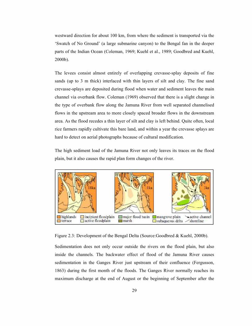
This sedimentation compensates the high subsidence rate of Bangladesh, thereby
keeping the river courses and the Bengal coastline relatively stable. The development
of the Bengal Delta over the last 18000 yrs is sketched in Figure 2.3. During this
period, the Brahmaputra River has switched its course several times between its
present course and the pre-1800 course.
According to Allison (1998), 21% of the annual sediment budget (mostly sand and
silt) is deposited at the river mouth, thereby enlarging the sub aerial delta with an
average of 4–7 km2 of new land over the last 150–200 years. Another 12.5% (mud) is
deposited further seaward as a subaqueous mud delta. Whereas the delta extends in
the eastern part, the shoreline and shallow offshore areas of the western front are in a
net erosional state (Allison, 1998). Net sediment transport along the coast is in
Page 46
29
westward direction for about 100 km, from where the sediment is transported via the
‘Swatch of No Ground’ (a large submarine canyon) to the Bengal fan in the deeper
parts of the Indian Ocean (Coleman, 1969; Kuehl et al., 1989; Goodbred and Kuehl,
2000b).
The levees consist almost entirely of overlapping crevasse-splay deposits of fine
sands (up to 3 m thick) interlaced with thin layers of silt and clay. The fine sand
crevasse-splays are deposited during flood when water and sediment leaves the main
channel via overbank flow. Coleman (1969) observed that there is a slight change in
the type of overbank flow along the Jamuna River from well separated channelised
flows in the upstream area to more closely spaced broader flows in the downstream
area. As the flood recedes a thin layer of silt and clay is left behind. Quite often, local
rice farmers rapidly cultivate this bare land, and within a year the crevasse splays are
hard to detect on aerial photographs because of cultural modification.
The high sediment load of the Jamuna River not only leaves its traces on the flood
plain, but it also causes the rapid plan form changes of the river.
Figure 2.3: Development of the Bengal Delta (Source:Goodbred & Kuehl, 2000b).
Sedimentation does not only occur outside the rivers on the flood plain, but also
inside the channels. The backwater effect of flood of the Jamuna River causes
sedimentation in the Ganges River just upstream of their confluence (Fergusson,
1863) during the first month of the floods. The Ganges River normally reaches its
maximum discharge at the end of August or the beginning of September after the
Page 47
30
main peak of the Jamuna River; its flood clears out most of the deposited sediments.
When the third flood peak of the Jamuna River is low or late, deposition can be
expected in the lower reaches of the Jamuna River near Aricha (Coleman, 1969)
Tracking plan form changes in detail for a dynamic river like the Jamuna River is a
challenging task. In the above figure the flow is shown from top to bottom. Hatched
areas indicate missing data (Figure 2.4). The size of the Jamuna River and the extent
of the surrounding flood plain make field surveys very time consuming. Therefore,
whenever a field survey is carried out, only a limited area is covered. The
development of remote sensing techniques has, on the other hand, made it possible to
obtain relatively detailed data by means of contemporary remote sensing satellite
systems because of the size of this river. Based on different combinations of signal
strengths over the detection bands, different types of land use can be detected. the
main branches of the all available years is shown on the left hand side of the figure.
Some lines are regularly revisited; in particular the northwest-southeast line at
northing 790 is remarkable. At that location the main branches of 1973, 1978 and
1980 (flowing out to the southeast) are in almost perfect alignment with the main
branches of 1994, 1995 and 1996 (coming in from the northwest). The underlying
cause may be related to tectonic influence; there are more of such indications as
(Mosselman et al., 1995) showed. At other locations the main channel seems to be
able to shift its direction but not its location (for instance at the Jamuna Bridge site).
For further analysis of the plan form changes, (EGIS, 1997) digitized the channel
centerlines from satellite images for 13 years between 1973 and 1995; the result of
1995 is shown on the right hand side in (Figure 2.5). They have distinguished one
main branch (in general the widest) and several secondary branches. An overlay of
these locations generally referred to as stable or nodal points of the braided plan form
are sometimes characterized by a different composition of the bank material resulting
in smaller erodibility. Although the migration rate may be reduced locally, these
‘stable points’ have shown to be transient on longer time scales. Satellite imaging
systems are very useful for quickly determining land use and channel plan form over
vast areas, but accurate elevation data are less easily although very time consuming,
Page 48
31
often still the best source for elevation data. Remote sensing methods for obtaining
elevation data are quick and efficient (Klees et al., 1997 a, b).
Page 49
32
Figure 2.4: Low-stage plan forms of the Jamuna River (Source: Jagers, 2003)
Page 50
33
Figure 2.5: Movement of the main channel for the period 1973-1995 and plan
form in 1995 (Source: EGIS).
A completely different way of obtaining elevation data has been used by (EGIS,
1997). Based on satellite images, they distinguished three types of land use: water,
Page 51
34
sand, and other land. Sand pixels correspond in the densely populated Bangladesh to
recently deposited (low lying) sand flats. The average elevation of sand covered
areas was - based on elevation data obtained from cross-section surveys at several
locations along the Jamuna River - determined to be 3.5 ± 1.0 m above SLW.
For the other land areas the elevation was correlated to the uninterrupted period that
the area had been classified as ‘other land’ immediately preceding the date at which
the latest satellite images and elevation data were obtained. They found the following
relation between the average elevation in meters above SLW and the land age in
years ����� � = 5.6 − 1.9����� �� , which is also plotted in (Figure 2.6). This
relation predicted three quarters of the calibration set within 1 m of the measured
height. Using this relation a DEM (digital elevation model) was created for the flood
plains in 1994 from which subsequently the plan forms at various characteristic
discharges were determined (Figure 2.7).
Figure 2.6: Relation between the elevation and the age of the land along the
Jamuna River (Source: EGIS, 1997)
The plan forms have been constructed by EGIS (1997) using low-stage satellite
images and field data by the River Survey Project (1996). Wash load does not play a
role in the reshaping of the bed and deposits of the sediment can only be found in
stagnant areas within the channel system.
Page 52
35
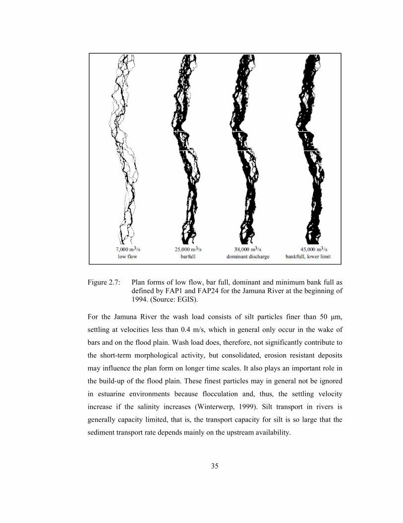
Figure 2.7: Plan forms of low flow, bar full, dominant and minimum bank full as
defined by FAP1 and FAP24 for the Jamuna River at the beginning of
1994. (Source: EGIS).
For the Jamuna River the wash load consists of silt particles finer than 50 μm,
settling at velocities less than 0.4 m/s, which in general only occur in the wake of
bars and on the flood plain. Wash load does, therefore, not significantly contribute to
the short-term morphological activity, but consolidated, erosion resistant deposits
may influence the plan form on longer time scales. It also plays an important role in
the build-up of the flood plain. These finest particles may in general not be ignored
in estuarine environments because flocculation and, thus, the settling velocity
increase if the salinity increases (Winterwerp, 1999). Silt transport in rivers is
generally capacity limited, that is, the transport capacity for silt is so large that the
sediment transport rate depends mainly on the upstream availability.
Page 53
36
2.7 Previous studies on different rivers
Numerous studies have done on the hydro-morphological aspects such as hydraulic
geometry, erosion/deposition and bed level variations in many rivers in Bangladesh.
Most of these studies were carried out in the major rivers like the Ganges, the
Brahmaputra, the Meghna and the Teesta River.
2.7.1 Studies in Bangladesh
Ali et al. (2002) investigated the effect of the changes in the planform and bed
topography of the Jamuna River in the form of a stability analysis by perturbation
technique. A two-dimensional model is developed and applied to the Jamuna River
which accesses flow and sediment transport in an alluvial river with erodible and
non-erodible banks. The proposed model is used to analyze both the meandering and
braided patterns of the river. The results from the analyses of the Jamuna River show
that instability always exists in the Jamuna River under maximum instability
conditions because of its very low aspect ratio (1/1000) and more than three braids.
The observation of Bristlow (1987) from satellite images suggested that the yearly
volume of erosion and deposition in the Jamuna is the function of the high discharge
and the duration of discharge. Bristow subdivided identified depositional areas from
satellite images into four categories: addition to bars, lateral accretion to the bank,
new mid channel bars and channel abandonment. Each types of deposition results
into the other types of erosion, say for example abandonment of an old channel is the
subsequent result of the formation of a new channel. Formation of a new medial bar
results in the widening of a channel by bank or bar erosion.
The riverbed erosion and deposition in the Jamuna River was first studied by
Coleman (1969). He found that due to high sediment load the erosion – deposition in
the riverbed is extremely high and the processes are very complicated. His study was
mainly based on the shifting of the thalweg, which is always associated with erosion
and deposition in the riverbed, by comparing cross-sectional profiles measured
Page 54
37
several times in a year at a certain section of the river, and by comparing each cross-
section measured in two successive lean seasons at different locations in the river.
Hossain (1989) studied the erosion – deposition pattern, shifting characteristics and
rate of change of cross-section and thalweg movement, including sediment transport
of the Ganges. He found that the net deposition in the Ganges up to Brahmaputra
confluence was approximately 4.26 X 10⁸ m
3 during 1967-68 to 1979-80 which
corresponds to about 4.30 cm sediment deposition each year.
Hossain and Alam (1988) performed a quantitative evaluation of sediment transport
rates in the Jamuna River and for that a comparative treatment of the applicability of
few well known formulae were made. They showed that total suspended sediment
discharge at Nakfatarchar was in between 439 million tons to 575 million tons and
94 percent of the flow occurs in the monsoon. They also found that sediment
discharge may satisfactorily be expressed as a function of water discharge and flow
velocity.
Habibullah (1987) studied the channel changes of the Jamuna over the time. He
found that the amount of bank line eroded is much higher than that accredited. He
also showed that maximum amounts of bank line erosion and deposition are 348
m/year and 335 m/year respectively.
Klassen and Masselink (1992) studied the bank erosion rate of the curved channels in
the Jamuna River by analyzing the satellite images from 1976 to 1987. As the
Jamuna River is a braided river, the various braided channels having different
discharges, width and radius of curvature are usually active in eroding the bank at
different places. They found that in the Jamuna River the bank erosion is generally
associated with the rotation and extension of bend rather than translation.
Mohammad A. H. Bhuiyan et al. (2010) evaluated the ongoing geoenvironmental
impacts of Brahmaputra-Jamuna (BJ) River around the Jamuna Bridge (JB) site.
Remote sensing and GIS techniques are adopted to evaluate the temporal and spatial
geohazards. This study shows that the intensity of channel shifting has been
Page 55
38
increased due to regulation of river width at Sirajganj–Bhuiyapur section from 11 km
to 4.8 km. Planform analysis shows that the major channel has been stressed to
migrate (315 m/year) eastwards.
Rahman (1978) had studied the erosion of the Padma River from Goalunda to
confluence of Padma-Meghna near Chandpur. He produced some relationships
between thalweg sinuosity with meander pattern.
Soni et al. (1980) conducted an experiment that covered a wide range of flow and
sediment loading conditions. They observed that after a long time, the aggradation in
downstream of the section of increased sediment supply was stopped once the
hydraulic conditions became compatible with the increased sediment load.
Analyzing satellite images, Thorne et al. (1993) estimated the bank erosion rate of
the right bank of the Jamuna River for the period of 1973-1992. They estimated bank
erosion at an interval of 500 m apart and averaged the erosion rate for 10 km. The
average bank erosion rate for the period 1973-1992 varies from 0 to 160 m/year and
the average erosion rate is about 80 m/year. They found that for a shorter time-scale
the bank erosion rate increases, and the average bank erosion rate is higher for a
higher flood discharges. They also found that catastrophic events of bank erosion (>
350 m/year) generally occur for short duration, 2 to 4 years and this erosion took
place at the outer bank of the curved cannels.
Thorne and Osman (1988) attempted to predict the bank erosion rate for the right
bank of the Jamuna River for different locations, extrapolating the previous results.
2.7.2 Studies around the world
Over the past decades several studies have been made to evaluate morphological
changes of the major rivers in and outside of Bangladesh. Although the list provided
is not exhaustive, yet it provides some information in this respect.
Jain (1989) proposed a guide for estimating river bed degradation. The rate and
extent river bed degradation resulting from sediment interruption were determined by
Page 56
39
means of computer based numerical experiment. He presented the results in the form
of algebraic relations that can be easily applied by practicing Engineers to estimate
the temporal and optimal river bed degradation during the preliminary phase of the
engineering designs. The proposed relationship for the bed degradation has been
verified with the field data of Missouri river.
Jaramillo and Jain (1984) performed investigations on the aggradation and
degradation of alluvial channel bed and introduced a one-dimensional nonlinear
parabolic model for non-equilibrium processes in the alluvial rivers. Their model can
be used as a tool for predicting aggradation-degradation processes in alluvial rivers.
Ramez et al. (2002) carried out a study on influence of sediment transport on the
computation of water in the river Rhone. They showed that the increase of the head
losses due to bed forms is interpreted in the U-curves (ratio of Strickler coefficients
versus ratio of bottom shear stresses) and of S-curves (Strickler coefficient versus
discharge). This effect is stronger at dominant discharge. It can lead to a rise of water
level much higher than the final topographical change. For the presented example of
a reach of River Rhône near Bourg lès Valence, this rise is estimated over 1 m for the
dominant discharge of about 1200 m3/s.
Ranga-Raju (1980) did a study on the practical computation of degradation and
aggradation on alluvial river based largely on the works carried out in India. He
presented semi-empirical methods for computation of bed and water surface profiles
for some of the commonly encountered cases of aggradation.
2.8. Mathematical modeling studies
Numerical hydrodynamic models of unsteady flow in rivers are widely used as an
engineering tool in the design and planning of water resources projects. In recent
years, several studies viz Master Plan Organization (MPO, 1987), Bangladesh Water
Development Board (BWDB, 1987), used the hydrodynamic as well as
morphological models of unsteady flow for computing flood flows and transport
rates for the rivers in Bangladesh. Besides Bangladesh due to invent of high speed
Page 57
40
computer nowadays, mathematical models are also extensively used for the
simulation of the natural processes all over the world.There are several methods in
numerical solutions i.e i) Method of Characteristics, ii) Finite Element Method, iii)
Finite Difference Method etc. Some of them are summarized below:
2.8.1 Studies in Bangladesh
Feasibility study for the Gorai River Restoration Project (GRRP) for augmenting dry
season flow through the Gorai off take had been taken-up by the Government of
Bangladesh (GoB) in 1997. A two-dimensional morphological model had been
developed for simulating the hydraulic and morphological processes in the Gorai off
take to study the feasibility of undertaking Gorai river restoration work. A quasi-
steady flow calculation was carried-out for the morphological calculation using
MIKE-21C of DHI Water and Environment. A helical flow module was used to
calculate the streamline curvature generated secondary flows. The sediment transport
computed are composed of bed-load and suspended load. For the bed load
calculation, the effects of the helical flow and bed slope were accounted through the
direction of bed-shear stress and direction of the bed-slope. The model was calibrated
and validated at the off take with extensive data collected for three consecutive
monsoons from 1998 to 2000. Both Chezy’s roughness (depth invariant) and depth
variant roughness were used in the study.
Jagers (2003) has focused on Modelling techniques to predict plan form changes of
braided rivers and their relation with state-of-the-art knowledge on the physical
processes and the availability of model input data. Three Modelling techniques have
been analysed with respect to their suitability for predicting plan form changes of
braided rivers: a neural network, a cellular model (Murray and Paola, 1994) and an
object-oriented approach (Klaassen et al., 1993). Two-dimensional depth-averaged
morphological simulations of sharp bends have been carried out to improve the
understanding of the processes involved. The results of those simulations indicate
that cutoff formation of Jamuna is accelerated by a low water level downstream, a
large(alluvial) roughness, a low threshold for sediment transport, and a small value
for the exponent c of the Shields parameter q (or of the velocity u) in the sediment
Page 58
41
transport relation if the average sediment transport rate remains constant. A simple
model concept for simulating head ward erosion has been presented and tested.
Finally, an algorithm for formation of new channels has been presented that can be
implemented as a new module in the branches model.
Analysis of the processed data revealed that formation of bars caused channel
bifurcation and created anabranches which together increased the total width of the
Jamuna from 7 km to 12 km over the study period. The anabranches thus created
either lost or gained with gradually. The one losing width ultimately becomes only a
remnant allowing the bar to merge with the flood plain.
The channel developed an oscillatory nature which erosion at the bank and the bar
developing a meander. He also revealed that the confluence has undergone an
oscillation due to the movement of the Ganges and formation of bars in the Jamuna.
This movement is estimated as 12 km within the study period.
Halcrow (2002) reviewed the morphological processes of the Jamuna River at Pabna
Irrigation Rural Development Project (PIRDP). Halcrow proposed riverbank
protection based on the morphological studies of the area. Three reaches of the bank
had been identified as susceptible to different degrees of erosion, and then the sites
were being prioritized to allow the introduction of a staged intervention program for
protecting the vulnerable bank reaches. A 4 km reach of bank line within PIRDP
showed immediate need for protection.
Houqe (1999) has studied the fluvial processes of the braided Jamuna in its 73.65 km
reach including confluence with the Ganges using application of remote sensing and
GIS. Using eleven sets of LANDSAT satellite images from 1973 to 1996, he studied
the bank erosion, meander travel, bar formations of Jamuna River and migration of
Jamuna-Ganges confluence.
In 2003, two models had been developed at IWM for finding a suitable location of
ferry ghat for BIWTA (Bangladesh Inland Water Transport Authority). For these two
models: one is a 30 km long and another one is a 200 km long reaches, where
Page 59
42
Jamuna-Ganges confluence had been included for both to study the erosion-
deposition pattern in the confluence region. The key features of the study were to
find a sustainable channel, which should have the minimum navigational depth round
the year. The short-model is used to evaluate the engineering interventions and the
long-model is used to simulate long-term bed level changes along the navigational
routes (BIWTA, 2003).
Two-dimensional model of Ganges River for Pakshey bridge project was developed
in 1999 by IWM and DHI (Danish Hydraulics Institute). The simulation was
developed using FESWMS-2DH model (version 3.0). FESWMS-2DH is an acronym
for finite element surface water Modelling system for two-dimensional flow in a
horizontal plane. It is a computer program to perform two-dimensional hydraulic
Modelling of rivers, floodplains and highway crossings. Main objectives of the study
were to find the impacts of the new bridge and river training works on the existing
Hardinge Bridge, river training works and the downstream irrigation intake canal and
also to evaluate the expected morphological changes in the river regime due to
proposed bridge.
2-D hydraulic model and morpho-dynamic model are developed by IWM in 1998
under the Meghna Estuary Study. The Meghna Estuary Study has covered an area of
the lower Meghna from Chandpur town up to the Bay of Bengal. The model has been
developed using Mike-21. The dominant hydraulic and morphologic conditions and
processes in the study area are studied through regional and detailed local 2-D
models. To determine the dynamic behaviour of the entire estuary system,
computations are carried out under different hydrodynamic conditions during low
and monsoon seasons. Neap tide and spring tide, current velocity and sediment
transport patterns and wave conditions are assessed in that study. The results of
these computations give qualitative and quantitative information about the spatial
and temporal variations of the water level, current velocity, discharge as well as
sediment transport and the rate of sedimentation and erosion.
A morphological model of Jamuna River at Jamuna bridge site was developed in
1995. The model was carried out by IWM (Institute of Water Modelling) using
Page 60
43
MIKE – 21C, which is a two-dimensional finite difference curvilinear grid model for
simulating hydrodynamic and sediment transport in vertically homogeneous flow.
The model covered a reach, extending 20 km upstream to 10 km downstream
approximately from bridge site. Bathymetry and hydrological data of the year 1994
were used in the model. Simulation of the hydrodynamics for pre-bridge and post-
bridge conditions was carried out for the entire monsoon period of 1994. Changes
from pre- to post bridge conditions have been extracted. The morpolological model
was run for one and a half month. The results showed that water level had increased
by 0.5m at the upstream of guide bund due to bridge construction.
BWDB (2011) initiated a project for protection of the left bank of the Padma River
from erosion at Bhagyakul Bazar, Baghra Bazar and Kobutorkhola under Sreenagar
Upazila of Munshigonj district. Institute of Water Modelling (IWM) carried out a
study using Mathematical Modelling tool MIKE – 21C in 2011 to ascertain hydro-
morphological design parameters of protection works of this project. The study
provides the identification of erosion trend of the vulnerable areas, devising suitable
options of river bank protection works, determination of maximum expected scour
level around river bank protection works, assessment of morphological changes in
the vicinity of the river bank protection works, assessment of river bank protection-
induced morphological changes, providing outline design of river bank protection
works, formulation of monitoring programm for the river bank protection works.
2.8.2 Studies around the world
A hydrodynamic and sediment transport model was developed in support of a
feasibility study for a port construction project in Dharma River, Orissa, India. The
proposed port had to be at the mouth of the Dharma River in the Bay of Bengal. This
would require development and maintenance of a 19 km long navigational channel,
and also a dike to divert Dharma river flow into the navigation channel to minimize
the maintenance dredging requirements. Tidal circulation and sediment transport
were modeled using RMA2 and SED2D.
Page 61
44
To study the meander migration and scour of the Roer River, a model had been
developed by Delft hydraulics for the Dutch Water Board. The main goal of the
project was to determine the migration velocity and migration development of the
meander bends, and the depth and velocity of the bed erosion of the Roer at the
location of tunnel. With the 1-D hydraulic and morphological model system SOBEK,
calculations were carried out to determine the large-scale morphological
development and the flood scour of the Roer at the tunnel location.
In order to demonstrate the impact of sediment supply on the morphology of Tenryuu
River (Japan), downstream of the Akida dam, Delft Hydraulics developed a two-
dimensional model using the Delft2D-River system. The activities included 2-D
schematization, extending the model system with the ‘Aishida’ and Michiue
sediment transport equations, hydraulic and morphological evolution of supplied
sediment volume.
Two-dimensional model was developed to examine the morphological effects and
changes in navigability of the Waal River due to lowering of groynes. This model
was developed with the help of Delft2D-River packages.
Hayter and Mehta (1986) demonstrated cohesive sediment related problems in
estuaries include shoaling in navigable waterways and water pollution. A two-
dimensional, depth-averaged, finite element (FE) cohesive sediment transport model,
CSTM-H, has been developed and may be used to assist in predicting the frequency
and quantity of dredging required to maintain navigable depths and the fate of
adsorbed pollutants. Algorithms which describe the processes of erosion, dispersive
transport, deposition, bed formation and bed consolidation are incorporated in
CSTM-H. The Galerkin weighted residual method is used to solve the advection-
dispersion equation with appropriate source/sink terms at each time step for the nodal
suspended sediment concentrations. The model yields stable and converging
solutions. Partial verification was carried out against a series of erosion-deposition
experiments in the laboratory using kaolinite and a natural mud as sediment.
Page 62
45
Nguyen et al. (2009) have studied a two-phase numerical model for suspended-
sediment transport in estuaries. They presented a full 2-D numerical model for
sediment transport in open channels and estuaries using a two-phase (fluid–solid
particle) approach. The physical concept and the mathematical background of the
model have given and test-cases have been carried out to validate the proposed
model. In order to illustrate its feasibility for a real estuary, the model has been
applied to simulate the suspended-sediment transport and the formation of turbidity
maximum in the Seine estuary. The numerical results show that the main
characteristics of estuarine hydro-sediment dynamics in the Seine estuary are in fact
reproduced by the proposed model. A qualitative agreement between the numerical
results and the actual observations has been obtained and presented in this study.
Shimizu and Itakura (1989) applied a two-dimensional model in calculating the bed
variation in alluvial channels. The model was applied to analyze the bed variations
with or without meso-scale bed configuration such as alternating bars (pool and
riffles) and braided bars, which can be observed even in straight channels.
Van Kessel (1999) carried out a number of tests on the performance of the non
cohesive (sand) formulations in the sediment version of Delft3D-FLOW. These tests
were carried out by Modelling a long (8km) straight flume with a movable sand bed.
The roughness and slope of the flume were such that a constant flow depth and
depth-averaged velocity were achieved along the length of the flume.
2.9 Summary
Several modeling studies have been conducted to till date to understand the behavior
of the different type of rivers in Bangladesh as well as over the world. But most of
these models are very expensive and some are very time consuming. On the other
hand Delft3D flow (FLOW), morphology (MOR) and wave (WAVE) modules are
available in open source and has proven its capabilities on many places around the
world, like the Netherlands, USA, Hong Kong, Singapore, Australia, Venice, etc.
(Delft3D Open Source Community). Delft3D is a powerful tool for the
understanding and forecasting of river morph dynamic behavior, because it takes into
Page 63
46
account the most relevant factors involved in this process (as input parameters) and
gives a broad range of results (as output parameters) presented in an accessible
manner. Jamuna is one of the largest rivers in Bangladesh. Every year the widening
of the river, bank erosion, development of large bars and deposition in main
navigational channels, are happened to be the major problems. On the basis of
background of the study and the literature review the main focus of the study is to
assess the morphology of the selected reach of the river by using the Delft3D
numerical model.
Page 64
47
CHAPTER 3
THEORY AND METHODOLOGY
3.1 General
Engineers have studied the subject of sediment transport for centuries. Different
approaches have been used for the development of sediment transport functions or
formulas. These formulas have been used for solving engineering and environmental
problems. Results obtained from different approaches often differ drastically from
each other and from observations in the field. Some of the basic concepts, their limits
of application, and the interrelationships among them have become clear to us only
in recent years. Many of the complex aspects of sediment transport are yet to be
understood, and they remain among the challenging subjects for future studies.
The mechanics of sediment transport for cohesive and non cohesive materials are
different. This chapter addresses non cohesive sediment transport only. This chapter
starts with a review of the basic concepts and approaches used in the derivation of
incipient motion criteria and sediment transport functions or formulas.
In Delft3D, the physical processes are modeled by a system of equations that consists
of two hydrodynamic equations, the continuity equation and the momentum
horizontal equations, and one transport equation for conservative constituents. In this
study the governing equations that Delft3D uses to model the hydrodynamic and
morphological changes of the river are described.
3.2 The basic equations of fluid dynamics
The basic equations of fluid flow, encode the familiar laws of mechanics:
• conservation of mass (the continuity equation)
• conservation of momentum
At the level of “fluid elements”, in any domain, the flow equations must be solved
subject to a set of conditions that act at the domain boundary.
Page 65
48
3.2.1 The Continuum Hypothesis - Fluid Elements
At a microscopic scale, fluid comprises individual molecules and its physical
properties (density, velocity, etc.) are violently non-uniform. However, the
phenomena studied in fluid dynamics are macroscopic, so instead of taking this
molecular detail into account, the fluid is treated as a continuum by viewing it at a
coarse enough scale that any “small” fluid element actually still contains very many
molecules.
3.2.2 The Continuity Equation
A volume V is considered bounded by a surface S that is fixed in space. This mass
inside it is given by � ���� , so the rate of decrease of mass in –
� = − ��� � ���� = − � ! � ��� … … … (3.1)
If mass is conserved, Eqn. 1 must equal the total rate of mass flux out of V. The rate
of outward mass flux across any small element �" of S is �. �", where the
magnitude of �" is equal to the element’s area. Integrating over the whole surface,
the rate of mass flux out of –
� = � �. �"% = � ∇. '�(��� … … ... (3.2)
The integrand ∇. '�( on the RHS is expressed in Cartesian coordinates x = (x, y, z),
v = (u, v, w) as –
∇. '�( = '!)( * + '!�( , + '!-( . … … … (3.3)
Figure 3.1 shows clearly that gradients in the flow field are required for non-zero net
flux. For mass to be conserved everywhere, Equation 3.1 and 3.2 must be equal for
any volume V and so the continuity equation –
! � + ∇. '�( = 0 … … … (3.4)
Page 66
49
Figure 3.1: Mass fluxes entering and leaving an element.
The Material Derivative
For any physical quantity f = f(x, t) (density, temperature, each velocity component,
etc.), the material (or substantive) derivative becomes –
/0/� = ��� 1'2'�(, 3'�(, 4'�(, �( = 0 � + �*�� 0 * + �,�� 0 , + �.�� 0 . = 0 � + 5 0 * + 0 , + 6 0 . = 0 � + . ∇1 … … …
(3.5)
Equation 3.5 conveys the intuitively obvious fact that, even in a time-independent
flow field ( 0 � = 0 everywhere), any given element can suffer changes in 1'. ∇1( as
it moves from place to place.
The continuity equation can also be written in the form –
/!/� + �∇. = 0 … … … (3.6)
If the fluid is incompressible, � = constant, independent of space and time, so
that /!/� = 0.
The continuity equation then reduces to
Page 67
50
∇. = 0 … … … (3.7)
which in Cartesian coordinates is
) * + � , + - . = 0 … … … (3.8)
The Delft3D-flow module similarly performs the hydrodynamic computations by
solving the Navier Stokes’ equations for shallow water in two (depth-averaged) or
three dimensions, under the hydrostatics pressure assumption, which neglects the
vertical acceleration due to buoyancy effects or changes in bottom topography
(Lesser et al. 2004).
The depth-averaged continuity equation is given by (Lesser et al. 2004):
7 � + 89:; * + 89<; , = " … … … (3.9)
Where, S represents the contribution of the discharge of water, = stands for the water
level and H is the water depth.
3.2.3 Conservation of Momentum
The Cauchy Equations
A volume V bounded by a material surface S that moves with the flow, always
containing the same material elements. Its momentum is � ���� , so the rate of
change of momentum = ��� � ��� =< � ��� /�/�< … … …
(3.10)
Stress tensor 8>;, defined so the force exerted per unit area across a surface element �" ≡ �@�" (by the fluid on the side to which �@ points on the fluid on the other side) is 1 = 8>;. �@.
Total force (body + surface)= � ���A +< � 8>;. �"B
Page 68
51
= � ��'�A + ∇. 8>;(< … … … (3.11)
By Newton’s second law, Eqns. 3.10 and 3.11 must be equal for any V, so the
Cauchy equation –
� /�/� = �A + ∇. 8>; … … … (3.12)
Figure 3.2: Surface stresses on a fluid element in 2 dimensions.
>CDis the force per unit area in the “i" direction across a plane with normal in the “j”
direction. As can be seen from (Figure 3.2), gradients in the stress tensor are needed
for there to be a net force on any element (consistent with the surface integral of 8>;. �@ equating to a volume integral of ∇. 8>;). It is possible to show that the stress
tensor is symmetric, i.e.
>*, = >,., >.* = >*., >,.E>., … … … (3.13)
Otherwise any small fluid element would suffer infinite angular acceleration.
Page 69
52
Constitutive Relations
The surface stresses 8>; on any element arise from a combination of pressure p and
viscous friction, as prescribed by the constitutive relations
>** = −F + G∇. + 2I ) * , >*, = I J ) , + � *K … … … (3.14)
>,, = −F + G∇. + 2I � , , >,. = I J � . + - ,K … … … (3.15)
>** = −F + G∇. + 2I - . , >*. = I J ) . + - * K … … … (3.16)
I and G are the coefficients of dynamic and bulk viscosity respectively.
Incompressible Navier-Stokes Equations
For incompressible flow, the constitutive relations reduce to –
>CD = −FLCD + I M )N *O + )O *NP … … … (3.17)
where v = (u1, u2, u3), x = (x1, x2, x3) and defined –
LCD = 1 �1 � = Q �� LCD = 0 �1 � ≠ Q
Inserting Eqn. 3.17 into Eqn. 3.12, assuming constant μ, and utilising again the
incompressibility condition 7, the incompressible Navier–Stokes (N–S) equations –
Continuity: 0 = ) * + � , + - .
Momentum, x: � /)/� = �A2 − S * + I J T) *T + T) ,T + T) .TK
Momentum, y: � /�/� = �A3 − S , + I J T� *T + T� ,T + T� .TK
Page 70
53
Momentum, z: � /-/� = �A4 − S . + I J T- *T + T- ,T + T- .T K … … … (3.18)
Or, in compact notation
Continuity: ∇. = 0 … … … (3.19)
Momentum: � /U/� = �A − ∇F + I∆U … … … (3.20)
In which ∆ is the Laplacian operator. For uniform �, the gravitational force is exactly
balanced by a pressure gradient ∇F0 = A that does not interact with any flow,
defining W = F − F0 gives –
� /U/� = −∇W + I∆U … … … (3.21)
Similar equation is followed by Delft3D
The momentum equation in X and Y direction are –
) � + )Z[\\ ) ] + �Z[^^
) _ + -�`7 ) a − �TZ[\\Z[^^
Z[^^ ] + )�Z[\\Z[^^ Z[\\ _ −
1 = − b!cZ[\\ W] + d] + b'�`7(T a Je ) aK + f]
� � + )Z[\\ � ] + �Z[^^
� _ + -�`7 � a − )TZ[\\Z[^^
Z[\\ _ + )�Z[\\Z[^^ Z[^^ ] + 15 =
− b!cZ[^^ W_ + d_ + b'�`7(T a Je � aK + f_ … … … (3.22)
Where e represents the vertical eddy viscosity coefficient. Density variations are
neglected, except in the baroclinic pressure terms, W] and W_ represent the pressure
gradients. The forces d] and d_ in the momentum equations represent the unbalance
of horizontal Reynold's stresses. f] and f_ represent the contributions due to
external sources or sinks of momentum (external forces by hydraulic structures,
discharge or withdrawal of water, wave stresses, etc.).
Page 71
54
3.3 Advection-Diffusion Equation
Delft3D calculates the transport of sediment by solving the three-dimensional
advection-diffusion equation for suspended particles (equation 3.3) (Deltares 2009).
In which, the flow velocities and eddy diffusivities are calculated from the
hydrodynamic equations 3.8 and 3.20. In addition, the program is able to adjust the
density of water in relation to temperature and salinity (Deltares 2009) and
differentiates the settling velocities and sediment fluxes between cohesive and non-
cohesive particles.
g � + :g * + :g , + '-�-h(g a − * Ji%,* g *K − , Ji%,, g ,K − a Ji%,. g aK = 0
… … … (3.23)
Where,
C = Depth averaged suspended sediment concentration [kg m-3
]
U, V = Flow velocity components in the x- and y- direction [m s-1
] 6% = Settling velocity [m s-1
] i%,*,,,. = Eddy diffusivities in three directions [m2 s-
1] '6 − 6%(= “assumption that the settling velocity with respect to the flowing water is
the same that in stagnant water” (Ribberink 2010).
The settling velocity for cohesive and non-cohesive sediment is calculated in relation
to the concentration (Deltares 2009). In high concentrations, the presence of other
particles reduces the settling velocity of a single particle.
3.4 Settling Velocity
The settling velocity of non-cohesive sediments can be modeled by the Van Rijn
(1993) formulation, which depends upon a representative sediment diameter, Ds. The
formulation is of relative importance for this study as the model is calibrated for the
Van Rijn’ 84 equation, which in Delft3D, requires the settling velocity as an input
value.
Page 72
55
6% = 6%,j =klmln '%�b(�/hTbo� ; 6ℎ�� 65 Ir < t% ≤ 100 Ir
bj�/h vJ1 + j.jb'%�b(�/hw�T K − 1x ; 6ℎ�� 100 Ir < t% ≤ 1000 Ir1.18'y − 1(At%;, ; 6ℎ�� t% > 1000 Ir{
… … …
(3.24)
And
t% = | 0.64t~j; 1 � � ≤ 1t~j�1 + 0.015'� − 25(�t~j; 1 � 25 ≤ � { ; 1 � 1 ≤ � ≤ 25 … … … (3.25)
s = relative density ρs/ρw of the suspended sediment fraction t% = representative diameter of sediment fraction [m] t~j = median grain size of bed material [m]
v = kinematic viscosity coefficient of water [m2 s
-1]
T = non-dimensional bed shear stress
3.5 Deposition and Erodibility on Delft3D
The model quantifies the sediment entering the flow due to an upward diffusion
(erosion) and the sediment dropping out of the water column due to the settling
velocity of particles (deposition). The sediment fluxes between the bed and flow are
based on modeled approximations by sink and source terms acting on a layer above
the reference height a developed by van Rijn (1993), named in Delft3D as the kmx
layer (Figure 3.3). The concentration approximation follows a standard Rouse profile
from the reference height a, to the centre of the kmx layer (Deltares 2009). Shortly,
the deposition and erosion flux through the kmx layer can be expressed as follows:
Deposition flux: t = 6%���* … … … (3.26)
Erosion flux: � ≈ i% Jg��g���∆. K … … … (3.27)
Page 73
56
Where, 6% = settling velocity [m s-1
] i% = sediment diffusion coefficient evaluated at the kmx layer. ���*= sediment concentration at the kmx layer [kg l-1
]
Δz = difference in elevation between the kmx layer and the van Rijn’s reference
height a [m]
Figure 3.3: Schematization of flux on the kmx layer (Deltares 2009)
Each half time-step the source and sink terms model the quantity of sediment
entering the flow due to upward diffusion from the reference level and the quantity
of sediment dropping out of the flow due to sediment settling. A sink term is solved
implicitly in the advection diffusion equation, whereas a source term is solved
explicitly. The required sink and source terms for the kmx layer are calculated as
follows.
Erosive flux due to upward diffusion
�'�( = i%'�( g'�( . … … … (3.28)
where i%'�( and
g'�( . are evaluated at the bottom of the kmx layer.
The erosion flux is split in a source and sink term:
Page 74
57
�'�( ≈ �T'�( �h'�( g�'�(∆. − �T'�( �h'�( g���'�(
∆. … …. …. (3.29)
��'�( correction factor for sediment concentration
i%'�( sediment diffusion coeffcient evaluated at the bottom of the kmx cell of sediment
fraction '�(
��'�( reference concentration of sediment fraction'�(
���*'�( average concentration of the kmx cell of sediment fraction '�(
∆4 difference in elevation between the centre of the kmx cell and Van Rijn's
reference height
" 5������%C��'�( = �T'�( �h'�( g�'�(∆. … … … (3.30)
"������%C��'�( = �T'�( �h'�( g���'�(∆. … … … (3.31)
Deposition flux due to sediment settling
The deposition flux is approximated by:
t'�( ≈ �b'�(���*'�( 6%'�( … … … (3.32)
This results in a simple deposition sink term:
"�����S�%C�C��'�( = �b'�(���*'�( 6%'�( … … … (3.33)
The total source and sink terms is given by:
" 5���'�( = ��'�(��'�( M�h'�(∆. P … … … (3.34)
Page 75
58
"���'�( = ���'�( M�h'�(∆. P + �b'�(6%'�(� ���*'�(
… … … (3.35)
where 6%'�(and ���*'�( are evaluated at the bottom of the kmx layer
These source and sink terms are both guaranteed to be positive.
Regarding the calculation of the sediment transport, Delft3D allows the combined
use of cohesive and non-cohesive sediment. By default, the formulations of Van Rijn
are applied for the suspended and bed load transport of non-cohesive sediment,
which is the case of the sandy sediment in the area of the selected reach. If desired, it
is possible to use other sediment transport formulae for non-cohesive sediment;
however it has been decided to stick to Van Rijn’s approach, because it is the most
used in other studies involving Delft3D, hence the most experienced and functional.
Due to the fact that sand transport models are often based on semi-empirical
equilibrium transport formulae that relate sediment fluxes to physical properties,
such as velocity, depth and grain size, it is crucial to perform sensitivity analysis of
the formulae used.
Pinto et al. (2006) compared four sediment transport formulations considering only
the tidal current only: Ackers and White (1973); Engelund and Hansen (1967); van
Rijn (1984 a,b,c) and Karim and Kennedy (1990). The authors concluded that the
van Rijn formula is the most sensitive to basic physical properties. Hence, it should
only be used when physical properties are known with precision.
3.6 Sediment Transport
3.6.1 Suspended and Bed Load Transport
The bed evolution is based on the sediment continuity (Equation 3.28), where the
first term expresses the changes in bed level in time (Tonnon et al. 2007) and the
second and third terms are the sediment fluxes (bed and suspended load) in the x-
Page 76
59
and y- directions, respectively. The equation states that the bed level evolution in
time is depended on the suspended and bed load gradients in the x and y directions.
.� � + �B�,�`Bh,�� * + �B�,�`Bh,�� , = 0 … . … (3.36)
Where,
"�,*,, = bed-load transport in x- and y-direction [kg m-1
s-1
] "%,*,, = sediment-load transport in x- and y-direction [kg m-1
s-1
] 4� = bed level [m]
The suspended and bed load transport are computed by standard sediment transport
formulations (Van Rijn (1993), Engelund-Hansen (1967), Bijker (1971), Soulsby,
etc), which subsequently are corrected for bed-slope effects, upwind bed
compositions and sediment availability (Deltares 2009). The Van Rijn’ 84
formulation is able to calculate the suspended and bed load transport separately and
distinguishes between the transport modes according to the reference height. Above
the reference height the concentration is catalogued as suspended load and below as
bed load. In river systems, as the particles are bigger, the settling velocity of particles
is higher than in other aquatic systems, the latter can be confirmed with the aid of the
Rouse Number P, which is a non-dimensional number that defines the transport
mode of the sediment. (Equation 3.29)
W = -h�)∗
W > 2.5 ��� � �0.8 < W < 1.2 "5yF����� � �W < 0.8 �yℎ � � … … … (3.37)
Where,
5∗ = Critical shear velocity [m s-1
]
k = von karman constant, typically 0.40 6% = Settling velocity, (0.1 m/s, calibrated Delft3D model) [m s-1
]
Page 77
60
According to the Van Rijn’ 84 formulation (Deltares 2009), the critical shear velocity
u* is determined by:
5∗ = ¡0¢�o … … … (3.38)
where,
q = Depth average velocity, 1 m s-1
1g� = friction factor expressed as (Deltares 2009)
1g� = j.�£v¤¥¦§cJ §T¨w©ªcKxT … … … (3.39)
with H = water depth
and t«j = 1.5t~j
3.6.2 Bed Load Transport: Van Rijn’ 84
For simulation without waves, the magnitude of the bed load transport is calculated
according to Van Rijn’ 84 equation, for which the model is calibrated:
"� = ¬ Z'y − 1(At~j�c.cw t∗�j.���.b, 1 � � < 3.0Z'y − 1(At~j�c.§ t∗�j.��b.~, 1 � � ≥ 3.0 { … … … (3.40)
Where, "� is the bed load transport rate [kg m-1
s-1
] and t∗ and T are the shear
velocity, non-dimensional particle size and the non-dimensional bed-shear stress
respectively (Van Rijn’ 84), with –
t∗ Non-dimensional particle size:
t∗ = t~j v'%�b(��T x§w … …. … (3.41)
T Non-dimensional bed-shear stress:
Page 78
61
� = ¯¢°�¢�°¢±°¢± … … … (3.42)
In which, the critical bed shear stress ²g� is written based on the Shields parameter
which is defined as a function of the non-dimensional particle parametert∗:
²g� = '�% − �(At~j³g�
³g� =klmln 0.24t∗�b, 1 � 1 < t∗ < 40.14t∗�j.´£, 1 � 4 < t∗ < 100.04t∗�j.b, 1 � 10 < t∗ < 200.013t∗�b, 1 � 20 < t∗ < 1500.055, t∗ > 150
{ … … … (3.43)
Where, the formulas to calculate the bed shear stress are:
²�g = bo �-1g� � … … … (3.44)
Where Ig is the reference level, for which the given calibrated model assumes a
value of 0.3 m and in which the Chézy coefficient C’ is expressed as a function of
the grain size D90, interpreted in Delft3D as 1.5D50. The equation is written as:
Ig = µbo ¤¥¦J§T¨\¢ K¶· ¸� … … … (3.45)
1g� = j.�£v¤¥¦§cJ §T¹w©ªcKxT … … … (3.46)
º» = 18 log J b�¿�/ªcK … … … (3.47)
The 2D-Chézy coefficient C can be determined with the following formulations:
Chezy formulation: º = Chezy coefÇicient Ërb �� y� Ì
Manning formulation: º = √¿Î�
Page 79
62
White Colebrook’s formulation: º = 18 logbj Jb�¿�h K
Where,
h = total water depth [m]
n = Manning coefficient Ërb �� y� Ì
�% = Nikuradse roughness length [m]
The general Modelling approach in Delft3D is that hydrodynamic flow is calculated
on a boundary fitted grid to which bathymetry, initial conditions and boundary
conditions are applied. Sediment transports are calculated following the flow and
wave field, according to the applied sediment transport formula.
Figure 3.4: Schematic overview Delft3D calculation steps (Source:Roelvink, 2006)
Variations in sediment transports in their turn determine the morphological
development of the model. The processes of flow, waves, sediment transport and
morphological updating are all executed at each time step according to the ‘online’
approach (Roelvink, 2006, Figure 3.4).
3.7 Methodological Steps
At first the study area has been defined using a satellite image of Pre monsoon 2010.
Then the boundaries of the study areas are defined by using the data of left and right
Page 80
63
bank of Jamuna for April 2010 of the selected 50 km reach. The land boundary is
obtained from GIS and the bathymetry is obtained using the Delft3D- QUICKIN
module. The bathymetry is interpolated to the grid nodes by triangulation
interpolation method. Once the grid is generated, various parameters such as
boundary conditions, roughness, eddy viscosity, initial conditions, time step,
sediment characteristics etc are assigned using the Flow module of Delft. Flow GUI
saves all the files required to run different modules of Delft3D.
3.8 Profile of the study area
The study reach is selected within the district of Sirajganj and Tangail from E463400
m to E486500 m and N680000 m to N730000 m (BTM coordinate) and covers about
50 km reach of the Jamuna River (30km upstream and 20km downstream of The
Bangabandhu Multi-purpose Bridge). Kazipur is situated at the right side at the
upstream end and Chauhali is situated at the downstream end of the study reach.
Balkuchi and Sirajganj on the right bank and Gopalpur and Bhuapur on the left bank
are other important places to be considered along the study reach. The location of the
study area is shown in Figure 3.5.
There are number of river training and bank protection works on the both bank of the
river in the study area. These are comprised of the Bangabandhu Multi-purpose
Bridge river training works (RTW) and BWDB bank protection works.
Page 81
64
Figure 3.5: Study Area on the Jamuna River (Source: IWM, 2010)
The river reach is characterized by well defined braiding nature, meta-stable islands,
nodes, sandbars, shifting ana-branches and rigorous bank erosion. Geo-
morphologically, the eastern bank is bounded with the lateral extension of Madhupur
Page 82
65
Tract and the west bank is the Barind Tract, which is composed of silty clay.
Topographically, the study area is part of alluvial plains (low land) formed by the
sediments of river and its tributaries and distributaries. The study area belongs to
region: floodplains and sub-region: Jamuna floodplain. The sub-region can be again
subdivided into the Bangali-Karatoya floodplain, Jamuna-Dhaleshwari floodplain,
anddiyaras and chars (Source: Banglapedia). The soil and topography of chars and
diyaras vary considerably. Some of the largest ones have point bars. The elevation
between the lowest and highest points of these accretions may be as much as 5 m.
3.9 Data Collection and Analysis
In order to determine the trend of the critical hydro-morphological conditions of the
Jamuna River Historical as well as most recent hydro-morphological data (pre-
monsoon 2011) have been Collected by IWM covering the distance between Kazipur
situated at the upstream end and Chauhali situated at the downstream 50 km reach of
Jamuna River incorporating all infrastructures including guide bunds and adjacent
hard points of Bangabandhu Bridge.
The secondary data for the present study has been collected from Bangladesh Water
Development Board (BWDB) and IWM. A number of reconnaissance surveys in pre
monsoon 2011 were done by IWM survey team. The survey concluded cross-section,
bank line and water level. The water level data of 2010 has been collected from
BWDB.
3.9.1 Satellite Image Data
Satellite images for the Jamuna River have been collected from Institute of Water
Modelling (IWM). The image is needed to extract the actual bank line of selected is
for assessment of bank line shifting and also in generating computational grid of the
model.
Page 83
66
3.9.2 Description of the selected stations
For Monitoring of Hydraulic and Morphological Conditions of Jamuna River for the
Safety of Bangabandhu Bridge as well as hydro-morphological forecasts of the river
at the critical locations within the bridge area for monsoon 2011, IWM collected data
during December 2010 - January 2011 for the stated 50 km reach from Kazipara to
Chauhali. Cross Sectional data of the particular reach have been collected at an
interval of 500 m for the first 10 km, then reduced to 250 m for 11 to 35 km and
again increased at an interval of 500m for 35 to 50 km.
3.10 Approach and methodology followed during data collection
3.10.1 Coordinate System
The position (x,y) of the data points has been received from the GPS is in
Bangladesh Transverse Mercator (BTM).
3.10.2 Bench Mark
For connecting water level gauges in the study area the existing and temporary
Bench Marks (TBM) established by different organizations have been used.
3.10.3 Bathymetric Survey
In the flowing region of the river the bathymetric survey has been conducted by the
survey boat. Digital echo sounder and the DGPS have been used to measure the
water depths and positions of the vessels successively. Staff gauges were used to
record the Simultaneous water levels relative to the datum (mPWD) with a known
gauge zero level at upstream and downstream of the survey reach.
3.10.4 Char Survey
Conventional optical levels (fly leveling) has been used in surveying the dry area.
Page 84
67
3.10.5 Bankline (Alignment) Survey
The alignment survey has been carried out by ProXR GPS (DGPS). At selected time
intervals the GPS position (northing & easting) of the alignment of the bank line is
continuously stored in the data logger.
3.10.6 Water Level Gauging
Water level gauges were established along the right bank of the Jamuna to conduct
the bathymetry survey. Daily 3 hourly water levels have been recorded from 06:00
hour to 18:00 hour. The gauges have been connected to the PWD datum from the
known reference BM/TBM by direct fly leveling.
Figure 3.6: Water level gauge on the River Jamuna
The river bank alignment has been surveyed for a total length of 67 km on both the
right and left banks. Easting, northing and the length are contained in the alignment
data.
A standard quality control procedure was maintained for all survey and data
collections.
3.11 Data Analysis
For understanding the morphological condition of the Brahmaputra Jamuna River,
two years cross-sectional data are taken. Also to know the long term morphological
Page 85
68
behavior of Brahmaputra Jamuna River flexible integrated Modeling suite Delft3D
software, which simulates two-dimensional (in either the horizontal or a vertical
plane) and three- dimensional flow is used. Delft3D consists of a number of well-
tested and validated programs, which are linked and integrated with one-another. The
GUI allows visualizing model input, reference data and simulation results as time
series and animations of two and three-dimensional data sets. It is a well proven tool
for hydrological and morphological model calculation. Additional pre and post
processing tools (such as the QUICKIN tool, a powerful editor of grid related data is
used to simulate the water level of the Sirajgonj station for all the time steps entered
on the Flow GUI and also shows the simulated bed level changes after 1 to 2 years
for the every cross sections.
In case of second objective, the two years cross-sectional data 2010-2011 are used.
The observed bed levels are extracted from the cross-sections of the bathymetry data
given by IWM by using of the Arc GIS Software which have been used to compare
with the simulated results.
To calibrate the model data of water level versus time for the months of monsoon (1-
4-2010 to 30-7-2010) are inserted in table A.1. From table A.1 a graph is plotted
showing a better result for calibration. And for validate the model data of water level
versus date and time for another two months of monsoon (27-4-2011 to 27-6-2011)
are inserted in table A.2. From table A.2 a graph is plotted showing a better result for
validation.
For the last objective, the comparison of the simulated result that is the model output
of Delft3D model, with the output of Mike 21 has been done. In these case the
observed data of 2011 has been used.
Page 86
69
3.12 Mathematical Modeling
3.12.1 Grid Generation
Steady hydrodynamic module is the foundation of all models. Grid generated under
this model is used for rest of the models. Grid generation is the most important task
in any model application.
In this study the curvilinear grid has been used that are created, modified and
visualized by Delft3D-RGFGRID module. Curvilinear grids are applied in finite
difference models to provide a high grid resolution in the area of interest and a low
resolution elsewhere, thus saving computational effort.
The generated grid points in M-direction and in N-direction are 299 and 146
respectively. The size of individual grid is (124 X 171) m2. Bathymetry of the grid
was to be assigned. Before any further development, mesh quality has been checked
to obtain a suitable and accurate solution. Various criteria has been checked, these
include: orthogonality, aspect ratio, courant number, grid smoothness and resolution
to minimize truncation errors in the finite difference scheme.
3.12.2 Bathymetry Generation
The study area was developed with good quality grids and then surveyed bathymetric
data were interpolated into those mesh nodes Normally bathymetric survey has been
carried out in the flowing part of the river The survey boat moved across the river
approximately in straight lines following pre-set transect lines, measured the water
depths and the corresponding positions. The depth schematization may be uniform or
non-uniform across the model area. A non uniform (space-varying) bathymetry is
given in an attribute file. Bathymetry has been developed under known parameter
settings.
Page 87
70
3.12.3 Sensitivity Analysis
Different parameter mainly the eddy viscosity and manning’s roughness coefficient
has been tested with entering different values as input for checking the sensitivity of
the model.
3.12.4 Calibration and Validation of the Model
During model development, many uncertainties exists related to input as model
geometry, boundary conditions, roughness, eddy viscosity etc. which can have
momentous impact on model solutions. Once geometry and boundary conditions
have been obtained with reasonable accuracy from the field, it is common practice to
set them out of preview of the calibration process. Validation is a multi-step process
of model adjustments and comparisons, leavened with careful consideration of both
the model and the data. During validation, a new set of observed data have been
incorporated to justify whether the calibrated parameters produces satisfactory result
for a new condition.
3.12.4.1 Hydrodynamic Calibration
For hydrodynamic calibration, mostly roughness and eddy viscosity are the
parameters to play with to obtain an adequate match with the observed field
conditions. For the present study, the water levels at Sirajgonj station located 30 m
upstream of Kazipur were compared with the simulated water levels of the model for
the same location. Due to lack of data of the dry season the calibration was
undertaken only for the wet season for 2 months (20 April 2010 to 28 June2010).
The roughness parameter (Manning’s n) was adjusted to get the best result.
3.12.4.2 Hydrodynamic Validation
The computed water surface elevations by the model were validated with observed
water surface elevations at Sirajgonj station for the months of 3 April 2011 to 14
August 2011. Good agreement between the observed and simulated water levels
indicates satisfactory performance of the model. During the calibration and
Page 88
71
validation process, the model showed good agreement with observed data for wet
periods. Therefore the model was capable to simulate different conditions and
scenarios used in the present study.
During the calibration and validation process, the model showed good agreement
with the observed data for the monsoon periods. For the lack of data for dry season it
was not possible to calibrate and validate for dry seasons.
3.12.5 Simulation of the Model
When satisfactory results are obtained in calibration and validation, the model was
considered ready for simulation and various analyses. First the model was run for the
base period of year 2010. The model was simulated for the two consecutive years
2011 and 2012 to predict the hydraulic and morphologic responses of the river. The
analysis was carried out for the river profile as well as for the selected cross sections.
3.13 Summary
This chapter comprehensively reviews and evaluates basic approaches and theories
used in the determination of non cohesive sediment transport rate. The step by step
methods conducted in this study is also discussed. Delft 3D models the
hydrodynamics processes according to the continuity and momentum equation,
whereas, the transport of sediment is modeled by the three-dimensional advection-
diffusion equation. The settling velocity for non-cohesive sediment is modeled in
Delft 3D according to the Van Rijn’ 93 formulation, which depends upon the
sediment concentration and the representative sediment diameter Ds, function of the
median grain size D50. The model quantifies the amount of sediment entering the
water column due to an upward diffusion (erosion) and a downward settling velocity
(deposition) passing through the kmx layer.
In this study, the Van Rijn’ 84 equation for bed load transport is utilized. The
formula is commonly used for situations without waves and calculates the bed load
transport rate according to the non-dimensional particle size.
Page 89
72
CHAPTER 4
MODEL SETUP
4.1 General
The study of natural river changes and the interference of man in natural water
bodies is a difficult but important activity, as increasing and shifting populations
place more demands on the natural sources of fresh water. Although the basic
mechanical principles for these studies are well established, a complete analytical
solution is not known but for the most basic cases. The complexities of the flow
movement and its interaction with its boundaries, which are themselves deformable,
have precluded the development of closed form solutions to the governing equations
that describe the mechanical behavior of fluid and solid-fluid mixtures. As a result,
alternative techniques have been developed to provide quantitative predictions of
these phenomena as an aid to engineering projects and river restoration efforts.
Modelling is one such technique. There are two types of models: mathematical
models and physical models (sometimes also called scale models).
Numerical modeling has become very popular in the past few decades, mainly due to
the increasing availability of more powerful and affordable computing platforms.
Much progress has been made, particularly in the fields of sediment transport, water
quality, and multidimensional fluid flow and turbulence. Graphical user interfaces,
automatic grid generators, geographic information systems, and improved data
collection techniques (such as LiDAR, Light Distancing and Ranging) promise to
further expedite the use of numerical models as a popular tool for solving river
engineering problems.
4.2 Numerical Model
The problem at hand cannot be solved directly for the prototype in numerical models.
The process from prototype data to the modeling and to final interpretation of the
results (i.e., the modeling cycle) is complex and prone to many errors. Careful
Page 90
73
engineering judgment must be exercised at every step. The modeling cycle is
schematically represented in (Figure 4.2).
Figure 4.1: Computer Modeling cycle from prototype to the Modeling results
The prototype is the reality to be studied. It is defined by data and by knowledge.
The data represents boundary conditions, such as bathymetry, water discharges,
sediment particle size distributions, vegetation types, etc. The knowledge contains
the physical processes that are known to determine the system's behavior, such as
flow turbulence, sediment transport mechanisms, mixing processes, etc.
Understanding the prototype and data collection constitute the first step of the cycle.
In the first interpretation step, all the relevant physical processes that were identified
in the prototype are translated into governing equations that are compiled into the
mathematical model. A mathematical model, therefore, constitutes the first
approximation to the problem. It is the prerequisite for a numerical model.
Next, a solution step is required to solve the mathematical model. The numerical
model embodies the numerical techniques used to solve the set of governing
equations that forms the mathematical model.
Another solution step involves the solution of the numerical model in a computer and
provides the results of modeling. This step embodies further approximations and
simplifications, such as those associated with unknown boundary conditions,
imprecise bathymetry, unknown water and or sediment discharges, friction factors,
etc.
Page 91
74
Finally, the data needs to be interpreted and placed in the appropriate prototype
context. This last step closes the modeling cycle and ultimately provides the answer
to the problem that drives the modeling efforts.
4.3 Description of the model used in this study
Delft3D is a software developed by WL | Delft Hydraulics, which provides a
multidisciplinary approach and numerical Modeling for coastal, river and estuarine
areas. It simulates in two (either in the horizontal or a vertical plane) and three-
dimensions the time and space variations of six phenomena and their
interconnections: flows, sediment transports, waves, water quality, morphological
developments and ecology; and it is capable of handling the interactions between
those processes. To achieve this, Delft3D consists of several modules, grouped
around a mutual interface, which are linked and capable to interact among them.
However, the modules can also run independently of one-another. These modules
which are used in this study are:
Hydrodynamics module (FLOW)
This module basically simulates non-steady flows in relatively shallow water. It
incorporates the effects of tides, winds, air pressure, density (due to salinity and
temperature) differences, waves, turbulence and drying and flooding of tidal flats.
The output of the module is used in all the other modules of Delft3D.
Sediment transport module (SED)
This module simulates the transport, erosion and settling of cohesive and non-
cohesive, organic or inorganic, suspended or bed sediments.
Morphodynamic module (MOR)
With the feedback of bottom changes to the hydrodynamic computation this module
execute bottom changes due to sediment transport gradients and user defined, time
dependent boundary conditions. Both wind and waves act as driving forces and a
Page 92
75
number of transport formulae have been built in. An essential feature of this module
is the dynamic feedback with the FLOW and WAVE modules, which allow the
hydrodynamic flows and waves to adjust them to the local bathymetry and permits
for forecasts on any time scale.
Figure 4.2: Interaction among the main Delft3D modules
Delft3D is integrated software, which implies that its aggregate performance is more
comprehensive than that of the sum of its individual components. When simulating a
water system, for instance, currents, morphology and water quality are accounted for
by inter-related modules, allowing for continuous feedback between those
phenomena, just as occurs in nature. A special Graphical User Interface (GUI) has
been designed to allow the interaction between the user and the modules in a friendly
manner preventing misinterpretations and/or lack of information. Also, the GUI is
used for the data entry and management, visualization of model data and control of
actual model runs, by a menu shell through which it is possible to access the various
modules. Furthermore, there are a number of tools and utilities for pre and post-
processing, from which the most used in this research are:
Page 93
76
RGFGRID
RGFGRID is a graphical program for generation and manipulation of grids, allowing
the generation of orthogonal, curvilinear grids of variable grid size for the
computations. The variable grid sizes allow for a high resolution in the area of
interest and a lower resolution far away at the model boundaries, thus saving
computational effort. Furthermore, the grid lines may be curved to follow land
boundaries and channels smoothly, avoiding the so-called stair-case boundaries that
may induce artificial diffusion.
The grid-generator RGFGRID is designed so that grids can be created and modified
with minimum effort, fulfilling the requirements of smoothness and orthogonality.
Various grid manipulation options are provided in order to fine tune the grid. All
operations are incorporated in a graphical interface, providing easy control of the
grid generation process.
QUICKIN
QUICKIN is a graphical program for interpolation and modification of bathymetric
data to the form accepted by the Delft3D modules. Often the depth samples (raw
data) are originated from various sources, each of different date, quality and
resolution. In order not to contaminate high quality samples with low quality
samples, QUICKIN allows for subsequent loading of data sets.
The FLOW and WAVE modules use equations that in fact are averaged over the grid
dimensions. Therefore, the best results are obtained if the model bathymetry
approximates the real bathymetry in an averaged sense rather than in a local sense.
Thus, if the sample resolution is higher than the grid resolution, an averaging method
is required. On the other hand, if there are less sample points than grid points, a
triangulation interpolation method is preferred. The various interpolation methods
and step-by-step approach of generating an optimal model bathymetry are operated
from a graphical user interface.
Page 94
77
QUICKPLOT
QUICKPLOT is a post-processing program used to visualize the outcome of
different simulation processes, with the possibility of a graphical and/or numerical
representation of the results. QUICKPLOT allows uniform access to all types of data
files produced by the Delft3D modules, to select and visualize computational results
and measured data.
Figure 4.3: Structure of Delft3D
4.4 Modeling framework
For the objectives of this research, only the FLOW modules and MOR modules have
been used. In fact, in this case the MOR module is not working as an independent
unit, but as a morphology extension integrated to the FLOW module. Thus, the
sediment transport option in FLOW allows the use of several of the existing
functionalities in the MOR module has been used.
During the simulation, the FLOW module calculates non-steady flow and transport
phenomena that result from tidal and meteorological forcing on a rectilinear or a
curvilinear, boundary fitted grid (previously generated using RGFGRID). The
hydrodynamic conditions (velocities, water elevations, density, salinity, vertical eddy
viscosity and vertical eddy diffusivity) calculated in the FLOW module is used as
input to the MOR modules.
The MOR module integrates the effects of waves, currents and sediment transport on
morphological developments, which are used for the next simulation of the FLOW
Page 95
78
modules. This is a cyclical routine that can be modeled as a hierarchical tree structure
of processes, the process tree, in which time intervals for the elementary processes
are defined. Processes may be executed a fixed number of times, for a given time
span or until some condition is met. The link between the involved process modules
(FLOW and MOR) occurs via a dynamic coupling. This allows a feedback between
the processes which can affect water flow and sediment movement.
4.5 Space and time variation
Physical phenomena vary on space and time, therefore a dimensional description of
the natural processes is required for an accurate representation of the reality. The
numerical hydrodynamic modeling system FLOW solves the unsteady shallow water
equations in two (depth-averaged) or in three dimensions. The system of equations
consists of the horizontal equations of motion, the continuity equation, and the
transport equations for conservative constituents.
In this case, to model the morphological conditions in Jamuna River, it has been
decided to use a time dependent, two-dimensional approach, because the sediment
transport, which is the process of interest for this study, can efficiently and accurately
be modeled in 2D. Besides, 2D modeling requires less computational time, therefore
allowing more test-runs for the calibration as well as for the representation of
multiple scenarios.
Furthermore, the variation of time scales for the diverse natural processes (ranging
from the order of hours or days in the hydrodynamic simulations, to the order of
months and years in the morphological simulations) represents a difficulty for the
integrated modeling of such processes. Long morphological simulations are achieved
by using the morphological time scale factor that scales up the speed of the changes
in the morphology to a rate that it begins to have a significant impact on the
hydrodynamic flows. The implementation of the morphological time scale factor is
achieved by simply multiplying the erosion and deposition fluxes from the bed to the
flow and vice-versa by this scale factor, at each computational time-step. This allows
Page 96
79
accelerated bed-level changes to be incorporated dynamically into the hydrodynamic
flow calculations.
4.6 Model Set-Up
To set-up Delft3D, as for any numerical model, one of the most important factors is
to analyze and prepare the input data, mainly physical conditions. This task demands
reliable and enough data to obtain accurate results, and the process of transforming
the available data to the input format required is time consuming. The various types
of data and information needed to operate the model are entered through the user
interface GUI, and are stored in several input files that can be modified manually by
editing the files, or by means of the GUI.
Considering the information available, it has been decided to prepare three different
basic set-ups for the Delft3D model, including:
- Set-up for April 2010: As initial set up to run the model
- Set-up of December 2010: For hydrodynamic calibration
- Set-up of September 2011: For hydrodynamic validation
Most complete available data (such as bathymetries) is for the year 2010, therefore
the other basic set-ups are based on 2010 data when needed, as well as in some
extrapolations of existing data. Moreover, Set-up 2010 includes all the information
retrieve during the visit to Jamuna and is the source set-up for the Modeling of the
final scenarios of this study. Based on these considerations, the set-up process is
described in the following sections.
4.6.1 Land Boundaries
At the first step land boundaries are generated for the different set-ups. The land
boundary represents the land-water marking, i.e. the boundary between land and
water. Land boundaries are only useful visual indications, and have no influence in
the computations of the model. (Figure 4.6.1)
Page 97
80
Figure 4.4: Land Boundary for selected reach of Jamuna River
4.6.2 Grid set up of the study reach
The grids were created that represent the area of study, and that provide the cells for
the numerical computation. This process is done manually using the grid generator
program RGFGRID, taking the land boundary as a reference to fit with the grid, and
considering an area wide enough to avoid unreliable shadows and disturbed data in
the grid open-boundaries, which can affect the area of study (Figure 4.6.2)
Chauhali
Downstream
Boundary
Kazipara
Page 98
81
Figure 4.5: Flow grids for selected reach of Jamuna River
4.6.3 Refine Grid
An important task is to refine the grid in the areas of interest, such as the bridge
location, hard points the eroded/accreted beaches and the surf zone (main area for
long shore sediment transport), where it is essential to have more resolution and a
finer computation. In (Figure 4.6.3), the refinement of the grid has been done near to
the Sirajgonj and Bhuapur Hard points and also near the bridge location.
Groynes
Page 99
82
Figure 4.6: Grids Refinement for selected reach of Jamuna River
4.6.4 Orthogonalise Grid
Next the grid has been orthogonalised (cells as rectangular as possible) in order to
fulfill the Delft3D computational requirement of orthogonality for the well
functioning of the model. This has shown in (Figure 4.6.4), of the cosine values of
grid corners. The cosine values should be close to zero. The error in the computed
direction of the pressure term in Delft3D-FLOW is proportional to these values. In
offshore areas the orthogonality should be less than 0.02. Near closed boundaries,
higher values are sometimes acceptable. (Delft-RGFGRID - User Manual). In the
study reach, it can be seen that the value in the inner model has been kept in range of
0 to 0.03, which is an acceptable limit for well functioning of the model.
Chauhali
Downstream
Boundary
Kajipara
Upstream
Boundary
Bangabandhu
Bridge
Sirajganj
Page 100
83
Figure 4.7: Orthogonality of grids for selected reach of Jamuna River
4.6.5 Grid Smoothness (Aspect Ratio)
The quality of a grid is to a large extent determined by its orthogonality and the rate
with which certain properties change over the area to be modeled (smoothness). A
measure for the grid smoothness is the aspect ratio of grid cells (ratio of the grid cell
dimension in M- and N-direction) and the ratio of neighboring grid cell dimensions.
Ratio of M-size/N-size, value ≥ 1. Must be in the range [1,2] unless the flow is
predominantly along one of the grid lines. In the modeled reach in (Figure 4.6.5), the
value varied in the range [1 to 1.66], which is in the acceptance range of DELFT
model.
Kazipara
Upstream Boundary
Chauhali
Downstream
Boundary
Page 101
84
Figure 4.8: Aspect ratio of grids for selected reach of Jamuna River
4.6.6 Bathymetry Development
The developed bathymetry of the study area is shown in (Figure 4.6.5). Grid can be
generated using the observed bathymetric points. But grid generated in this way
would not give better quality model. Hence, the study area has been developed with
good quality grids and then surveyed bathymetric data are interpolated into those
mesh nodes. Normally triangular interpolation has been used but other methods are
also available under Delft-Quickin program. Before the interpolation process to
select the active interpolation area, a polygon has been generated. From the toolbar
the edit option has been clicked then selected the polygon. Furthermore, the
bathymetry has been smoothed by operating the depth smoothing option.
Page 102
85
IWM lean period bathymetry data surveyed during April 2010 has been used to set-
up the initial bathymetry of the model. The distribution of measured and interpolated
bathymetries is shown in (Figure 4.6.5) and (Figure 4.6.6).
Figure 4.9: Measured Bathymetry used in the model
Page 103
86
Figure 4.10: Interpolated Bathymetry used in the model
4.7 Flow Module Set-Up
Setting-up the FLOW model has been done through the user interface GUI of the
FLOW module. In the first stage a description of the project and the selection of the
grid file and the depth file (bathymetry) have been done. The location of the project
(latitude and orientation) is also a requested data in order to consider the influence of
the Coriolis force (for Jamuna: 24.39996 dec. deg N, 0 dec. deg W). Afterwards the
following aspects have been taken into account.
Page 104
87
4.7.1 Dry Points and Thin Dams
To represent structures that interfere and influence the hydrodynamic computations,
FLOW comprises the concept of dry points and thin dams. The main difference
between them is that dry points are grid cells that are permanently dry during a
computation irrespective of the local water depth, whereas thin dams are infinitely
thin objects that prohibit flow exchange between two adjacent computational cells
without reducing the total wet surface and the volume of the model. The purpose of a
thin dam is to represent small obstacles (e.g. breakwaters, dams) in the model, which
have sub-grid dimensions, but large enough to influence the local flow pattern. In the
present study groynes has been provided and constricted the area near the
Bangabandhu Bridge. The model grid in the groins area has been refined previously
in the Delft3D QUICKIN module to get better resolution. The disadvantage is that,
every time the grid is modified, many other input files must be modified as well,
such as depth files, observation points and cross sections. This is a weakness of
Delft3D model, because requires a lot of efforts and is time consuming.
4.7.2 Time Frame
For the simulations with FLOW, the hydrodynamic simulation time has been set to
122 days with a time step of 1 minute. The time step is important because for explicit
Modelling schemes such as Delft3D (where the unknown value of the dependent
variable at one time level is expressed as an explicit function of the known values of
the dependent variable at earlier time levels), the accuracy and numerical stability of
the model depends on the Courant Number defined as:
º� = � ∆�∆* … … … (4.7.2)
Where,
c = celerity ∆� = simulation time step ∆2 = grid size variation
Page 105
88
In general, Delft3D model is stable for Courant Numbers of 20 or lower;
nevertheless the model can work for higher Cr when, under the criteria of the
researcher, results are accurate and the calibration and validation process is
acceptable.
Figure 4.11: Courant Number variation as function of the grid size
4.7.3 Boundary Set Up
Boundaries are important as they define the input conditions to the Modelling
process within the grid. For the FLOW grid, four boundaries have been defined. It
consists of two open boundaries (Upstream and Downstream boundaries) and two
Chauhali
Downstream
Boundary
Kazipara
Upstream Boundary
Page 106
89
closed boundaries showing the bank lines. Normally total discharge is assigned at the
upstream inflow boundary and water level at downstream boundary. The model of
the Jamuna River had a total discharge boundary at the upstream Kazipur and a water
level boundary at downstream at Chauhali.
Figure 4.12: Flow Boundaries
Chauhali
Kazipara
Page 107
90
In Delft3D, boundary conditions can be assigned to every node or in line of that
boundary. The rating curve at Bahadurabad has been used to generate boundaries at
upstream northern end. Interpolated water level from Shirajganj has been applied to
downstream boundary. All the boundaries are applied for two distinct periods – for
the month of April 2010 to June 2010 during calibration and for four distinct
periods for the months of April 2011 to August 2011 during validation. The
discharge and water level hydrographs of these periods as shown in Figure 4.7.3 and
Figure 4.7.4 have been taken to apply into the model as boundary conditions and
subsequent calibration and validation purposes.
Figure 4.13: Time series hydrographs from April to July 2010 used in the model as
Boundary Conditions for Calibration Period
Boundary Conditions for Calibration Period (Year 2010)
0
10000
20000
30000
40000
50000
60000
70000
80000
1-Apr 21-Apr 11-May 31-May 20-Jun 10-Jul 30-Jul
Time (day)
Dis
charg
e (
m3/s
ec)
0
2
4
6
8
10
12
Wate
r Le
vel (m
PW
D)
Upstream Boundary - Discharge
Downstream Boundary - Water Level
Page 108
91
Figure 4.14: Time series hydrographs from April to October 2011 used in the
model as Boundary Conditions for Validation Period
In the year 2010 the water level rises abruptly during April to July as well as the
discharge also increased abruptly. Again in 2011 it can be observed from the
hydrograph that the water level raised abruptly during April to June, fluctuated
slightly during the next three months then slightly falls from the end of August
almost to the mid of September then again slightly raises in the end of September. In
case of discharge similarly abruptly discharge raised from April to July then slightly
fluctuated downward for the next three months, and falls rapidly during the end of
August to September. Several discharge peaks can often be observed due to the
dependence on rainfall and the distribution of the tributaries along the river in Assam
and Tibet.
4.7.4 Initial Conditions
Initial conditions, which state the hydrodynamic condition at the start of simulation,
need to be defined for all models. Usually the time series boundary conditions at
specified upstream and downstream ends are available from various sources. Other
than these, discharge or water level data at all the other points at model are not
Boundary Conditions for Validation Period (Year 2011)
0
10000
20000
30000
40000
50000
60000
1-Apr 1-May 31-May 30-Jun 30-Jul 29-Aug 28-Sep
Time (day)
Dis
charg
e (
m3/s
ec)
0
2
4
6
8
10
12
Wate
r Le
vel (m
PW
D)
Upstream Boundary - Discharge
Downstream Boundary - Water Level
Page 109
92
available. So, for defining the initial conditions at all the points at the model, it
becomes essential to run a steady hydrodynamic model with a specified discharge
and water level in defined upstream and downstream ends. The first steady run is a
cold-start, used when initial water levels for nodes other than the downstream
boundary are unknown. In cold start, initial downstream water surface elevation must
be provided in such a manner that all the mesh nodes of the model remain
submerged, otherwise the steady solution may diverge. For simplicity, the initial
water level for the whole domain was assumed same as the downstream water level
boundary condition, and accordingly velocity is assumed to be zero at all nodes.
Downstream water surface elevation is decreased gradually towards desired water
level boundary condition.
For the present study, as it has been intended to start simulation from 1st April 2010,
the water level has been found 5.27 m is chosen as our desired downstream
boundary. As such, 8944 m3/s inflow boundary discharge has been found
respectively for the corresponding downstream 5.27 mPWD water level. Once the
cold start solution is obtained, it is used as hot-start for other steady or unsteady
models.
4.7.5 Parameters in Hydrodynamic Flow Module
Various inputs and parameters contribute in adjusting the solution technique of the
hydrodynamic module of Delft3D. These are Eddy viscosity, bed resistance or
roughness parameter etc.
Table: 4.1 Hydraulic Parameters used in model
Parameters Values considered in the model
Roughness parameter (Manning’s, n) 0.014 for char and 0.025 for channel
Horizontal Eddy Viscosity 1
Vertical Eddy Viscosity 1
Page 110
93
The turbulence parameter coefficient of eddy viscosity is used for the distribution of
flow by exchanging lateral momentum of flow. In Delft3D, the eddy viscosity has
been specified 1 on the basis of several studies. (IWM, 2011)
Roughness parameter such as Manning’s ‘n’ is an important parameter in
hydrodynamic module since it provides some control over the fluid velocity
magnitude and direction.
The Manning’s ‘n’ is mainly a calibration parameter in the hydrodynamic module
and was taken in the range of .014 to .025 m1/2
/s based on various conditions of the
domain. Depth varying roughness has been used with the lower value of 0.025 where
the bathymetry depth is more than or equal to 6 mPWD and .014 where the depth is
below 6 mPWD (Mike 21C manual).
The morphological module is used to capture various morphological changes of the
river. This module simulates various features based on the results obtained during
hydrodynamic calculations. Various inputs and parameters associated with this
module are sediment transport predictors, alluvial resistance, grain size of soil etc.
Van Rijn formula was applied for Sediment transport prediction in this study. The
grain size of Jamuna River was taken 200 μm, reference density for hindered settling
1600 kg/m3, Specific density 2650 kg/m
3, Dry bed density 1600 kg/m
3, also the
initial bed layer thickness is taken uniform 5 m along the domain (IWM, 2011).
4.7.6. Morphological Updating
The elevation of the bed is dynamically updated at each computational time-step. At
each time-step, the change in the mass of bed material that has occurred as a result of
the sediment sink and source terms and transport gradients is calculated. This change
in mass is then translated into a bed level change based on the dry bed densities of
the various sediment fractions. Both the bed levels at the cell centers and cell
interfaces are updated. A number of additional features have been included in the
morphological updating routine in order to increase the flexibility.
Page 111
94
4.7.7 Morphological “Switch"
To specify to update the calculated depths to the bed MorUpd (or equivalently
BedUpd) flag in the morphology input file has been set. The use of MorUpd or
BedUpd only affects the updating of the depth values (at ζ and velocity points); the
amount of sediment available in the bed will still be updated.
Morphological data is quite important because it is the link between FLOW and
MOR modules. In fact, the MOR module is indirectly defined within the FLOW
input and therefore it is not necessary to go through an independent MOR set-up
process. Under the morphological data, the morphological scale factor is defined; in
this case the factor has been set to 8.25 for all the simulations which means that for a
hydrodynamic simulation time of 121 days the morphological time is approximately
equal to 1000 days (Approximately 33 months)
Under the numerical parameters, an important input is the smoothing time which is
the time that the model takes to stabilize the processes after the initial conditions of
the simulation. During this initial interval, the output of the model is inaccurate and
does not reflect the reality, this is why a smoothing time is necessary. In this case it
has been set to 60 minutes.
4.7.8 Monitoring Option
To monitor the evolution of the Modeling process it is possible to define observation
points and cross sections in which Delft3D will calculate and store the different
output variables. All the observation points and cross sections will be linked to an
output file and the results can be graphically displayed using QUICKPLOT. (Figure
4.7.5)
Page 112
95
Figure 4.15: Observation points and cross sections
Observation points are used to monitor the time-dependent behavior of one or all
computed quantities as a function of time at a specific location, e.g. water elevations,
velocities, fluxes, and concentration of the constituents among others. Observation
points represent an Eulerian viewpoint at the results. Observation points are located
at cell centers, i.e. at water level points. In the present study several observation
points has been selected near the Sirajgonj station for observing the value of the
simulated water level.
Cross-sections are used to store the sum of computed fluxes (hydrodynamic), flux
rates (hydrodynamic), fluxes of matter (if existing) and transport rates of matter (if
Page 113
96
existing) sequentially in time at a prescribed interval. A cross-section is defined
along a constant grid line and it must include at least two adjacent grid points. In the
present study 5 cross-sections has been selected. The location of each cross section
has been measured form upstream boundary.
4.8 Summary
Delft3D is a powerful tool for the understanding and forecasting of riverine and
coastal morphodynamic behavior, because it takes into account the most relevant
factors involved in this process (as input parameters) and gives a broad range of
results (as output parameters) presented in an accessible manner, using graphs with
the possibility to convert the results into text files. This allows the user to analyse
oceanographic variables such as waves, hydrodynamic variables such as flows,
morphologic variables such as sediment transport, and man-made variables such as
dredging and dumping volumes. (Delft3D-FLOW_User_Manual).
Page 114
97
RESULTS AND DISCUSSIONS
CHAPTER 5
5.1 General
This chapter presents the results of the hydrodynamic and morphological analysis of
the particular reach of Jamuna River, selected as study area by means of Delft3D
modeling. The simulation results of the mathematical modeling of this study area
have been analyzed and also compared with the field measurements, which have
assisted to acquire experience and knowledge regarding the changing nature of the
Jamuna River.
The aim of this present study is to observe the morphological changes of the selected
reach of the braided river Jamuna by using the Delft3D software and also to compare
the results obtained from the simulation with the field observations. The simulated
bed level changes compared with the field measurements, movement of bank line
and channel shifting at vulnerable locations as well as the aggradations and
degradation near chars and channels are some of the morphological events analyzed
in this chapter.
Erosion or deposition at any nodes points to the bed level lowering or rising,
respectively. However, it cannot automatically shift the bank-line when a bank node
gets erosion/deposition for itself. So any lowering of nodes at the bank, indicate the
bank at that location is vulnerable, which is supposed to produce bank erosion and
subsequent bank-line shifting. In this model vulnerable banks are identified by taking
several cross-sections at different locations of the model, where the bank nodes have
undergone lowering of its bed elevations.
Page 115
98
5.2 Model Calibration
5.2.1 Necessity of Model Calibration
Model calibration is the most important step in the overall model development. It is
an iterative adjustment of the model parameters so that simulated and observed
responses of the system match within the desired level of accuracy. In reality, all
models require some degree of calibration to fine tune the predictive ability of the
model. Without calibration it is not possible that any activities would produce
satisfactory solutions for real world situations. In a hydrodynamic model, errors may
occur in from four potential sources (Abramowitz and Stengun, 2003):
(i) Random or systematic error in input data,
(ii) Error due to incorrect parameter values and
(iii) Error due to incomplete or incorrect model formulation.
Errors from source (iii) are minimized, during the calibration process whereas the
mismatch between the simulated and observed outputs is due to all the four sources.
Errors related to (i) and (ii) determine the minimum level of disagreement between
the observed and simulated outputs. Hence, the objective of model calibration is to
minimize the errors from source (iii) until they become insignificant compared to the
errors from sources (i) and (ii). As far the fourth source is concerned, effort has to be
made to determine that the state equation, initial condition and boundary condition
have been specified correctly.
Usually parameters values are adjusted through ‘trial and error’ by running the model
repeatedly. Sound understanding of physical process of the phenomenon and
experience with similar real world systems can be of great help in determining the
correct parameters values. For a large number of parameters, it is not realistic to try
and adjust all the parameters one by one or in combination. A more sensible
approach is to attempt a coarser simulation using only a few parameters whose
values are least well known or to which the model shows maximum sensitivity
(Abramowitz and Stengun, 2003).
Page 116
99
5.2.2 Calibration Data
There are a number of uncertainties that exists related to input as model geometry,
boundary conditions, roughness, eddy viscosity etc, which can have momentous
impact on the model solutions. Once geometry and boundary conditions have been
obtained with reasonable accuracy from the field, it is common practice to set them
out of preview of the calibration process.
.
Figure 5.1: Comparison of simulated and measured water levels of Jamuna River
for calibration at Sirajganj
Roughness and eddy viscosity are the parameters that have been used to play to
obtain an adequate match with the observed field conditions in the present study.
Manning’s roughness coefficient has been adjusted after several trial of the model
during calibration to n = 0.014, when water depth is lower than 6 m and n = 0.025,
when water depth is higher than 6 m (Mike 21C manual). The value of eddy
viscosity has been considered as 1.0 (IWM, 2011). Calibration of the model has been
done using the set up of April 2010. For hydrodynamic calibration, computed water
surface elevations have been compared with the observed water surface elevations at
Page 117
100
Sirajganj station for the period of April to July, 2010. Calibration results showed that
the computed values are within ± 0.6 m (Figure 5.1).
5.3 Model Verification
5.3.1 Necessity of Model Verification
Most real world models contain a large number of parameters; it is not always
possible to produce a combination of parameters values which replicate the recorded
data satisfactorily. However, this does not ensure an adequate model formulation or
optimal parameter values. The calibration may have been achieved entirely by
numerical curve fitting without considering whether the parameter values so obtained
are physically reasonable. Moreover, it might be possible to achieve multiple
calibrations or apparently equally satisfactory calibrations based on different
combination of parameter values. It is therefore important to find out if a particular
calibration is satisfactory or which of the several calibrations is the best one by
testing (verifying) the model with a different set of data not used during calibration
(Halim and Faisal, 1995).
According to Klemes (1986), a simulation model should be tested to show how well
it can perform the task for which it is intended. Performance characteristics derived
from the calibration data set are insufficient as evidence of satisfactory model
operation. Thus the verified or validated data must not be the same as those used for
calibration but must represent a situation similar to that to which the model will be
applied operationally.
5.3.2 Verification Data
Once the model has been calibrated, the next step is to validate the model by
comparing the outputs to historical data from the study area. Validation is a multi–
step process of model adjustments and comparisons, leavened with careful
consideration of both the model and the data. The computed water surface elevations
by the model were validated with observed water surface elevations at Sirajganj
station for the period of April to August, 2011.
Page 118
101
Figure 5.2: Comparison of simulated and measured water levels of Jamuna for
validation at Sirajganj
During the calibration and validation process, the model has showed good agreement
with the observed data for the monsoon periods. For the lack of data during dry
season it has been not possible to calibrate and validate for dry seasons.
5.4 Simulation of the model
In this section Delft3D Flow module has been used for hydrodynamic and sediment
transport modeling. From the previous article we can see that the results have shown
satisfactory agreement during calibration and validation process. Hence the model
was considered to be ready for simulation and various analyses. At the beginning the
model had been run for the base period of year 2010. Initial bathymetry of April
2010 has been taken as base for simulation as shown in Figure 5.3. In this figure the
x-coordinate indicates the easting values and the y-coordinate indicates the northing
value of the selected sections of the study reach. Then to verify the result of the
observed and simulated bathymetry several cross sections are compared. The
observed and simulated bed levels at different cross-sections in December 2010 have
Page 119
102
been compared. The result showed a very good agreement. The model was then
simulated for predicting the hydraulic and morphologic responses of the river in the
years of 2011 and 2012.
Figure 5.3: Cross Sections shown in Bathymetry of selected reach of the Jamuna
River for comparison
5.4.1 Comparison of observed and simulated bed elevations
Sediment model simulated bathymetry of December 2010 is compared with the
observed bathymetry in December 2010. Comparisons at different cross-sections are
presented as the distance along cross-section versus bed elevations in mPWD
Sec a-a
Sec c-c
Sec b-b
Sec d-d
Sec e-e
Sec f-f
Sec g-g
West Guide
Bund
East Guide
Bund
Page 120
103
(Figure 5.4 to 5.10). From the results it is found that simulated bed elevations
adequately matched with the measured bed elevations.
Figure 5.4: Comparison of Cross-Section at (Sec a-a)
Figure 5.5: Comparison of Cross-Section at (Sec b-b)
0
2
4
6
8
10
12
14
16
18
0 5000 10000 15000 20000
Ele
vation (m
PW
D)
Distance from right bank (m)
Simulated Measured
0
2
4
6
8
10
12
14
16
18
0 5000 10000 15000 20000
Ele
vation (m
PW
D)
Distance from right bank (m)
Simulated Measured
Page 121
104
Figure 5.6: Comparison of Cross-Section at (Sec c-c)
Figure 5.7: Comparison of Cross-Section at (Sec d-d)
-4
-2
0
2
4
6
8
10
12
14
16
18
0 5000 10000 15000 20000
Ele
va
tion
(m
PW
D)
Distance from right bank (m)
Simulated Measured
0
2
4
6
8
10
12
14
16
18
0 2000 4000 6000 8000 10000 12000
Ele
va
tio
n (m
PW
D)
Distance from right bank (m)
Simulated Measured
Page 122
105
Figure 5.8: Comparison of Cross-Section at (Sec e-e)
Figure 5.9: Comparison of Cross-Section at (Sec f-f)
0
2
4
6
8
10
12
14
16
18
0 500 1000 1500 2000
Ele
va
tio
n (m
PW
D)
Distance from right bank (m)
Simulated Measured
0
2
4
6
8
10
12
14
16
18
0 500 1000 1500 2000 2500
Ele
va
tio
n (m
PW
D)
Distance from right bank (m)
Simulated Measured
Page 123
106
Figure 5.10: Comparison of Cross-Section at (Sec g-g)
5.4.2 Variation in Velocity and Sediment Transport
The series of figures below show the depth average velocity and the consequent total
transport of sediment of the study reach of the river Jamuna in both dry and wet
seasons. It can be visualize from the figures that during monsoon 2011 and 2012,
there is a higher velocity of flow in the main channels of the selected reach compared
to the dry period of 2011 and 2012. A light and deep blue area of (Figure 5.11 to
5.20) indicates relatively the lower erosion areas, while yellow and red colors
indicate higher erosion areas. The velocity seems to be high mainly near Sirajganj
Hard Point, Bangabandhu Bridge area (near East and West Guide Band),
Bahadurabad Hard point, Shubaghacha during both the monsoon and dry season.
These are the zones seem to get eroded. It is evident from the figures that the zones
with higher velocity carry more sediment than the other zones. From (Figure 5.11 to
5.20), it also can be noticed that the flow velocity increased in the successive years
similarly the amount of sediment transport has been increased. In eastern part of the
study reach, specifically near Bahadurabad it can be observed that the velocity of
flow is high in 2011 and respectively low in 2012 as a result the rate of sediment
-2
0
2
4
6
8
10
12
14
16
18
0 2000 4000 6000 8000 10000
Ele
va
tio
n (m
PW
D)
Distance from right bank (m)
Simulated Measured
Page 124
107
transport decreases hence some amount of deposition took place on that location.
Appearance of many distributary channel can be observed in 2011 and 2012, which
is much clearer in July 2012 due to higher flow velocity erosion took place and many
distributary channels appeared. The channels bifurcated from the Sirajganj station;
show lower flow velocity compared to other locations and consequently possesses
lower sediment transport capacity. Similar phenomena can be observed in the
downstream portion of the channel. In this zone the flow velocity increased in the
subsequent years as well as the sediment transport capacity.
Sediment transport capacities of the river are also responsible for the morphological
changes induced by erosion-deposition. If discharge is higher it produces greater
velocities as well as carries huge amount of sediment and there by increases the
sediment transport capacities of the river. The sediments are deposited in where the
velocity is low. As a result the bed level rises of the channel as observed in the
previous figures.
Page 125
108
Figure 5.11: Depth Averaged Velocity
in 29/7/2010
Figure 5.12: Total Sediment Transport in
29/7/2010
Page 126
109
Figure 5.13: Depth Averaged Velocity in
27/1/2011
Figure 5.14: Total Sediment Transport in
27/1/2011
Page 127
110
Figure 5.15: Depth Averaged Velocity in
27/7/2011
Figure 5.16: Total Sediment Transport in
27/7/2011
Page 128
111
Figure 5.17: Depth Averaged Velocity in
25/1/2012
Figure 5.18: Total Sediment Transport in
25/1/2012
Page 129
112
Figure 5.19: Depth Averaged Velocity in
24/7/2012 Figure 5.20: Total Sediment Transport in
24/7/2012
Page 130
113
The results obtained from the numerical modeling Delft3D shows that the depth
average velocities in the both east and west channel during the monsoon season of
the stated years are significantly higher compared to dry season.
The above figures show that the sediment transport of the river varies spatially and
this process is influenced by the local bathymetry and associated discharge and
velocity. In July 2010, the transport rate varies approximately between 0.005 m3/s/m
to 0.038 m3/s/m with an average of 0.0215 m
3/s/m. The average sediment transport
rates of the selected reach of the Jamuna River for various seasons are shown in
Table 5.1.
Table 5.1: Average Sediment transport rate of the river for various seasons
Seasons Sediment Transport Rate (m
3/s/m)
2011 2012
Dry 0.0065 .018
Wet 0.0065 .036
The variation of discharge, velocity and sediment transport capacities as mentioned
above affect the morphology of the Jamuna River. For various periods or seasons,
these variables change resulting in different morphologic responses of the river.
Deposition near the char areas, formation of deep pockets and development of deep
channels are the significant morphologic features. These processes can be better
understood by analyzing the selected cross sections on the river. These sections along
with their projected bed levels for different periods are shown in Figure 5.21.
The analysis was carried out for the river profile as well as for the selected cross
sections. The selected cross sections are shown in Figure 5.21. The locations of each
cross section measured from upstream boundary.
Page 131
114
Figure 5.21: Bathymetry of selected reach of the Jamuna River in April 2010
The series of Figure (5.22-5.25) reveal that the three morphological years have much
similar type of erosion and deposition patterns. Both erosion and deposition has been
occurred mainly in monsoon season.
Sec 2
Sec 1
Sec 3
Sec 5
C-1 C-2
Permanent Char
B- 1
Permanent Char
C-4 C-5
B-5
Sirajganj Hard
Point
Bhuapur Hard
Point
C-3
Page 132
115
Figure 5.22: Initial bed level in (1 April 2010)
Figure 5.23: Simulated bed level in (25 September 2010)
Page 133
116
Figure 5.25: Simulated bed level (28 September 2012)
Figure 5.24: Simulated bed level (23 September 2011)
Page 134
117
SECTION 1
Section 1 is located near upstream boundary at Kazipur (Figure 5.21). The main
channel is situated at the west side of the reach. A char has divided the channel into
two branch channel, indicated as C-1 and C-2. During the dry season this char
normally remains dry and flooded during monsoon season. There is also a permanent
char situated at the middle location of this section.
Figure 5.26: Cross-section at Section 1
In the beginning of the simulation in April 2010, it can be seen from the (Figure
5.22), that most of the flow was passing through the channel C-1. It is clear from the
Figures (5.23 to 5.25) that small amount of deposition took place on both side of the
char due to reduction of the velocity as well as increased the area and length of the
char. Both of the channels have undergone severe erosion due to increased velocity,
as a result they became relatively deeper and narrower. The bank of the channel C-1
has shifted westward and the bank of channel C-2 on eastward.
-15
-10
-5
0
5
10
15
20
25
30
0 5000 10000 15000 20000
Ele
va
tio
n (m
PW
D)
Distance from right bank (m)
Apr-10 25-Sep-10 23-Sep-11 28-Sep-12
Page 135
118
Cross Sections superimposed at section 1, shown in (Figure 5.26) for the period of
April 2010 to Sept 2012, also indicates the same findings that both the channels C-1
and C-2 had undergone around 5 m of erosion due to increase in magnitude of the
velocity from 2.38 m/s to 3.24 m/s and 1.6 m/s to 2.8 m/s respectively. Therefore
both banks are vulnerable due to the erosion in this location.
Besides this main channel consecutively many shallower and narrower channel has
been developed on the left side of the permanent char due to velocity fluctuations up
to September 2011 but there is no change on the right side of the permanent char.
Therefore no erosion and deposition took place up to September 2011, as there was
no flow velocity. But in September 2012, it can be seen that both erosion and
deposition took place on both side of the permanent char as some velocity of flow
has been observed and consecutively shallower and narrower channel appeared.
SECTION 2
In section 2, the main channel C-1 due to meandering nature has taken a shifting in a
sinuous manner from west to east direction (Figure 5.21). Also a branch channel
formed from this channel indicated as B-1 and connected with this channel again in
the downward direction. There is a char existing in between them (Fig 5.22).
Maximum flow is passing through the channel C-1 due to its bending nature and also
due to higher velocity than that of the branch channel B-1. Severe erosion took place
in both of the channels, thus relatively deeper and narrower channel has been created
in the subsequent years. The channels became narrower due to deposition took place
on both side of their banks as a result of reduction in flow velocity. From September
2011 to September 2012, erosion and deposition took place in between the main
channels alternatively. Therefore a huge amount of deeper but narrower channel has
been appeared in this location; another branch channel can be seen formed from
channel C-1 in the year 2012. Also in the year 2012, due to increase in flow velocity,
few small tributary channels can be observed in the east side of the reach. Both of the
channels, C-1 and B-1 have shifted in westward from their bank lines.
Page 136
119
Figure 5.27: Cross-section at Section 2
From the superimposed cross sections at section 2 (Fig 5.27), it is clear that a
maximum erosion of 5 m has taken place in the channel C-1 and C-2 due to
increased velocity from 2.24 m/s to 2.98 m/s and 1.2 m/s to 2.3 m/s respectively.
SECTION 3
This section is located near Sirajgonj District (Figure 5.21). A major change can be
observed in the main channel. At the starting of the simulation in April 2010, the
channel was wide and shallow. A huge amount of erosion as well as shifting of the
channel can be observed in westward in September 2011 and 2012 (Fig 5.24 and
5.25). Although the channel has been shifted in eastward in September 2010 as
deposition took place on both of the bank lines, for reduction of the flow velocity
(Fig 5.23).
-15
-10
-5
0
5
10
15
20
25
30
0 5000 10000 15000 20000
Ele
va
tio
n (m
PW
D)
Distance from right bank (m)
Apr-10 25-Sep-10 23-Sep-11 28-Sep-12
Page 137
120
Figure 5.28: Cross-section at Section 3
Superimposed cross-sections in (Figure 5.28) also indicate the same findings. It is
found that about 5 m of erosion took place in the channel due to increased velocity
from 2.38 m/s to 3.77 m/s. In September 2012, a significant change has been
observed in both sides of the permanent char. Alternatively huge number of erosion
and deposition took place on both side of the chars due to continuous fluctuations of
two velocities. Hence the width of the char has decreased as well as the area. In the
location of erosions the existence of some tributary channel has been observed which
seems to be relatively shallower and narrower.
SECTION 4
This section is close to the multipurpose Bangabandhu Bridge . There exist two
branch channels created after passing the Sirajgonj indicated as C-3 and C-4. There
is also a small branch channel, appeared from the branch channel C-4 and again
connected with the same channel indicated as B-4 (Figure 5.21).
-15
-10
-5
0
5
10
15
20
0 5000 10000 15000
Ele
va
tio
n (m
PW
D)
Distance from right bank (m)
April_2010 25_Sep_2010 23_Sep_2011 28_Sep_2012
Page 138
121
Figure 5.29: Cross-section at Section 4
At the beginning of the simulation, it can be observed that the flow velocity in both
of the channels, C-3 and C-4 was low during the dry season. During the monsoon
period in the year 2010 and 2011, the widths of both the channels have been reduced.
Due to reduction of the velocity deposition took place on both of their respective
banks. Both the channels, C-3 and C-4 have been shifted towards east and west
respectively. But in 2012, the area influenced by the velocity is greater, thus much
erosion took place and the bank line of both the banks seems to be shifted in west
and east direction respectively. On the other hand, due to the tremendous flow
velocity, huge erosion took place in both channels. Thus deeper and narrower
channel has been formed up to 2011. A significant amount of erosion as well as
deposition can be observed in the year 2012, for which the bank lines of all the
channels have been shifted including the branch channel B-6 (Fig 5.25).
Superimposed cross-sections at section 4 (Fig 5.29) for the studied years also
indicate the same findings. The channels C-3, C-4 and B-1 have undergone a severe
-10
-5
0
5
10
15
0 1000 2000 3000 4000 5000 6000
Ele
va
tio
n (m
PW
D)
Distance from right bank (m)
April_2010 25_Sep_2010 23_Sep_2011 28_Sep_2012
Page 139
122
erosion of about 5 m in the year 2012 due to an increased flow velocity of about 2.34
m/s to 3.37 m/s, 2.36 m/s to 3.69 m/s and 0.84 m/s to 2.14 m/s respectively.
A char existed in between the channels C-3 and C-4. In September 2011, significant
erosion took place on both side of the char and deepened the branch channel B-1. But
in September 2012, it can be seen that a large amount of deposition of about 4 m
took place at right side of the char due to the reduction of flow velocity and the
branch channel has significantly shifted. Therefore the area of the char has been
increased.
SECTION 5
Section 5 is situated near to the downstream of the study reach near to Chauhali
(Figure 5.21). In this section, a major change has been observed in the main channel.
Severe erosion took place in September 2012 due to increase in flow velocity. In
September 2011, the magnitude of flow velocity is relatively lower than that of in the
year 2010 and deposition took place in some amount and reduced the deepness of the
channel compared to 2010 (Figure 5.30). It is evident from (Figure 5.23 and 5.24)
that alternatively erosion and deposition took place in September 2010 and 2011.
Hence there existed a temporary char in between them and divided the channel into
two branch channels, which are relatively deeper and narrower. Huge amount of
deposition took place in both side of the channel in September 2010 and
consequently the channel has shifted towards east. The channel has shifted towards
west in September 2011 and lastly in September 2012, due to more erosion and
increased velocity the temporary char has been completely eroded and deeper and
wider channel has been created.
Page 140
123
Figure 5.30: Cross-section at Section 5
From the cross section (Figure 5.30), it can be observed that around 5 m of erosion
took place and the velocity was 2.36 m/s. This velocity reduced to 2.05 m/s and then
increased abruptly to 3.22 m/s. In September 2010, a huge amount of deposition of
around 7.5 m and 3 m took place on both the left and right side of the channel due to
reduction of velocity at that location.
Table 5.2: Average Erosion and Deposition of Observed and Simulated Bathymetry
Cross-section Dec-10 Sep-11
Observed (m) Simulated (m) Observed (m) Simulated (m)
Section 1 -0.083 -0.003 -0.284 -0.182
Section 2 0.205 0.167 0.263 0.173
Section 3 0.002 0.003 -0.024 -0.039
Section 4 0.074 0.051 -0.882 -0.688
Section 5 -0.021 -0.052 -0.280 -0.354
-15
-10
-5
0
5
10
15
20
25
30
35
0 2000 4000 6000 8000 10000 12000
Ele
va
tio
n (m
PW
D)
Distance from right bank (m)
April_2010 25_Sep_2010 23_Sep_2011 28_Sep_2012
Page 141
124
The comparison of average erosion and deposition of observed and simulated cross-
sections for September 2011 and December 2010 has been shown in Table 5.2. The
result shows a very good agreement between observed and simulated bathymetry.
The maximum, minimum and net erosion and deposition of the study area of Jamuna
River during the simulated time period are summarized in Table 5.3.
Table 5.3: Bed Level Changes for the selected sections
Section
Maximum Deposition
(m)
Maximum Erosion
(m)
NetDeposition/Erosion
(m)
2010 2011 2012 2010 2011 2012 2010 2011 2012
1 2.23 5.91 5.41 -2.90 -4.99 -4.99 0.09 0.10 -.05
2 3.71 4.15 5.96 -3.90 -5.0 -5.0 0.14 0.16 0.28
3 2.53 8.58 9.74 -5.0 -5.0 -5.0 -0.17 -0.15 -0.17
4 10.36 3.73 5.22 -5.0 -5.0 -5.0 0.18 -0.46 -1.73
5 4.56 11.69 8.81 -1.69 -5.0 -5.0 0.06 0.07 -0.19
Page 142
125
5.4.3 Comparison of the simulated bathymetry in September 2011 by Mike21 and Delft 3D
Figure 5.31: Simulated bathymetry by Mike 21 (September 2011)
Figure 5.32: Simulated bathymetry by Delft 3D (September 2011)
Page 143
126
The above figures (middle portion of the selected reach) show the simulated images of
the bed level in September 2011. From Figure 5.32, it is found that Delft 3D model
predicted river bed degradation patterns near Sirajganj Hard Point and East Guide Bund
are very similar with the predicted river bed degradation of Mike 21 by IWM. From both
pictures it can be revealed that the range of colors is well adjusted. Aggregation can be
observed in the simulated bathymetry near the bank lines. But it can be observed that in
both the picture that the highly erosion affected zone are at the same locations Shirajgonj
and near the east guide bund of the main channel. In these zones according to the color
bar the values are below 0mPWD indicating the violet and deep blue zone successively.
The tributaries are in the range of 0 mPWD to 5 mPWD indicated by the light green
color. Also the big char areas are indicated in red and deep yellow color successively
ranging above 14mPWD.
5.5 Sensitivity Analysis
To determine the model’s performance and how the model responds to several
parameter settings a sensitivity analysis is performed. The sensitivity analysis consists of
several stages. First several runs with the default parameter settings were made and the
output is evaluated to check the general performance of the model. After these initial
computations, several computations were made with different parameter settings, to see
how these parameters influence the results. Parameter settings include:
• bottom roughness
• eddy viscosity.
5.5.1 Bottom roughness
In the Delft model the Manning parameter is varied to investigate the sensitivity of this
parameter on the discharge. Three runs are made with a Manning parameter for char and
channel (char 0.1 and channel .01; char 0.1 and channel .014; char .025 and channel
.014). It is clear from figure 6.1 that the Manning parameter (n) has rather large
influence on the water level, discharge constituents. When increasing the Manning
Page 144
127
parameter the bottom roughness increases, mainly it can be seen that the water level
height increases mainly due to the increase of the roughness of char rather than channel.
Fig. 5.33 Influence of Manning parameter on amplitudes of water level
The influence of the Manning parameter on of the water level in Shirajganj is also
noticeable. In figure 5.33 it has been observed that the height of the water level after
the run differ within 2.8m with the roughness n=0.1, .014, differ within 2.5m with n=0.1,
.01 and differ within .6m with n=0.025, .014. The run with n=0.1, .014 has the largest
difference from the observed water level data and the run with n=0.025, .014 is
relatively much close to the observed data.
Page 145
128
5.5.2 Eddy Viscosity
The next important parameter that has been tested in tuning the run is the eddy viscosity.
Three values have been taken to test the difference 1, 3 and 10. 10 is the default value
and 1 is the value used for the alluvial river from various studies (IWM, 2011). The
result for the three values has been shown in (figure 5.34). There is no such influence in
the model as the water level variation is almost same. Hence we have considered the
known used value 1.
Fig. 5.34 Influence of Eddy Viscosity on amplitudes of water level
5.6 Summary
In general the model shows very reasonable results, especially considered the many
uncertain factors in the model.
Page 146
129
A further improvement of the model is considered not feasible with the available data.
The most limiting factors are the lack of reliable bottom depths and reliable discharge
data. For the purpose of the study the created model is accurate enough to draw
conclusions.
Page 147
130
CONCLUSIONS AND RECOMMENDATION
CHAPTER 6
6.1 General
The numerical technique Delft 3D developed in this study has been applied in the
Jamuna river for a reach extending from Kazipara to Chauhali. Taking April 2010 field
data of bed level as reference bed level, the changes of bed level in the two successive
years within the reach has been computed by running the programme. The following
conclusions has been drawn from the present study
6.2 Conclusions
The summary of the findings of the present study for the selected reach of the Jamuna
River located at 30 km upstream and 20 km downstream from the Bangabandhu Bridge
are as follows:
1. The model developed in this study has been calibrated against the observed
water surface elevations at Shirajgonj. Attempt has been made to calibrate
only the high flow data as most of the morphological activities occur during
this period. Result obtained from the calibration process has shown adequate
agreement with the observed values.
2. Next the model has been validated for two months (April to June) during the
monsoon period with the water surface elevations of Shirajgonj. Result has
shown satisfactory matches between observed and simulated values.
3. The erosion and deposition for one year and then two successive years have
been computed, for the study reach using the present technique. It has been
found that more materials have deposited mostly adjacent to the char areas
which are surrounded by the channel branches. From the selected cross
sections it can be revealed that maximum deposition took place on 2012 that
Page 148
131
is about 9.97 m in section 1 near kazipur whereas maximum erosion took
place on all the sections of about 5m.
4. In the present study the sediment transport rate, erosion and deposition and
bed level changes has been analyzed for non cohesive sediment. The
simulated average sediment transport rate is 0.0065m3/s/m for dry season
and 0.0065m3/s/m for wet season in Sep 2011. In Sep 2012 the transport rate
is 0.018m3/s/m for dry season and 0.036m
3/s/m for wet season. Delft is
capable of analyzing the above parameters in case of cohesive sediment also.
5. Overall there has been a very small amount of deposition. Considering the
changes during the last two years and also along the total study reach of the
Jamuna River it has been seen that appreciable deposition is absent but there
has been a large amount of erosion in the west channel.
6. A relationship has been analyzed in variation of velocity and sediment
transport. It can be seen that due to increased velocity the rate of sediment
transport increases hence there forms erosion and the shifting characteristics
of the channels can be observed.
7. The plan form analysis has revealed that during the past two years the river
has shifted quite appreciable towards the east and west. The shifting process
of river course and its subsequent erosion and accretion processes cause the
loss and newly formation of land simultaneously.
6.3 Recommendations for further Study:
For getting better knowledge on the changes in the morphologic and hydrologic
conditions of the Jamuna River the following suggestions are made for further study and
to facilitate future studies:
1. There should be the availability of all types of data like discharge, water
level, sediment concentration, cross section that covers shorter time interval
and closer distance for both the dry and flood seasons.
Page 149
132
2. The discharge and water level data should be measured at more stations all
over the year to facilitate better understanding of morphological processes.
3. Nowadays the existence of multiple tools to model and evaluate all these
aspects, such as Delft3D into the technical field, are supportive elements to
generate numerous feasible scenarios and to select the optimal one
4. This type of morphological assessment studies can be carried out in most of
the major rivers, estuaries and coastal regions of our countries by using the
Delft Software.
5. There are some deficiencies in the functioning of the software which need to
be improved. For instance, it has been needed to manually adjust some input
files generated by the software tools RGFGRID and QUICKIN (e.g. delete
some lines in grid files). Besides, any change in the grid configuration means
the need to redo depths, cross- sections and observation points, which is time
consuming.
6. It is also complicated to define obstacles such as jetties, groins and
revetments, because they must be fitted to the grid points; thus it is
impossible to accurately define the exact position of these obstacles.
Besides, any change in the grid configuration means the need to redo depths,
obstacles, cross-sections and observation points, which is time consuming.
7. In the present study the bridge has not been considered as the resolution of
pier was difficult to adjust with the resolution of the grid.
Page 150
133
REFERENCES
1. Alam, M. K. and Hosain, M. M., 1988, “Sediment transport in the River
Jamuna”, Journal of Institution of Engineers, Bangladesh, Vol. 16, Issue 1-2, pp.
17-26.
2. Allison, M. A., 1998. “Historical changes in the Ganges-Brahmaputra Delta
front”, Journal of Coastal Research, pp. 1269–1275.
3. Ali, Md. Hazrat and Kyotoh, Harumichi, 2002, “Instability Analysis of the
Jamuna River, Bangladesh”, Pertanika J.Sci. & Technol., Vol. 10, pp. 229-250.
4. Bhuiyan, Mohammad A. H., Rakib, M. A., Takashi, Kumamoto, Rahman, M.
Julleh Jalalur, Suzuki, Shigeyuki, 2010, “Regulation of Brahmaputra-Jamuna
River around Jamuna Bridge Site, Bangladesh: Geoenvironmental Impacts”,
Journal of Water Resource and Protection, Vol.2, pp. 123-130.
5. Bian, C., 1998, “Scientific exploration of Yarlung Zangbo River grand canyon”,
Beijing, Vol. 41, Issue 13, pp. 21-22.
6. BIWTA, 2003, “Hydraulic and morphological study for the selection of a site for
ferry ghat alternative to Nagarbari/Notakhola”, Final Report prepared by
department of Water Resources Engineering, BRTC, BUET.
7. Bristow, C. S., 1987. “Brahmaputra River: Channel migration and deposition.”
In Ethridge et al. (1987), pp. 63–74.
8. BWDB, 1998, “Meghna Estuary Study”, Draft Master Plan, Vol. 2:
Morphological processes.
9. BWDB, 2011. "Bangladesh er Nod-Nodi", Bangladesh Water Development
Board (BWDB), Dhaka, Bangladesh.
10. Coleman, J. M., 1969, “Brahmaputra River: channel processes and
sedimentation,” Sedimentary Geology 3 (2–3): pp.129–239.
Page 151
134
11. DHI/SWMC., 1999, “Mathematical morphological model of Jamuna River at
Jamuna bridge site”, Final Report, Phase II, prepared by Danish Hydraulic
Institute in Association with SWMC.
12. DHI/SWMC., 1997, “Mathematical model study (Phase I) for optimizing of
dredging, Gorai River Restoration Project”, Final Report, Phase I, Danish
Hydraulic Institute in Association with SWMC.
13. EGIS, 1997, “Morphological dynamics of the Brahmaputra-Jamuna River”,
Tech. Rep., EGIS, Dhaka, Bangladesh.
14. FAP 1, 1994 “River training studies of the Brahmaputra river”, Master Plan
Report, Annex 4, Design and Construction, BWDB.
15. FAP21/22, 1994. Technical report No. 2: "Morphological predictions for test
areas, Bank protection and river training pilot project FAP21/22. FAP21/22,
Dhaka, Bangladesh.
16. FAP24, 1994. Study report No. 3: “Morphological studies phase 1”, Available
data and characteristics. FAP24, Dhaka, Bangladesh.
17. Fergusson, J., 1863. “Delta of the Ganges.” The Quarterly Journal of the
Geological Society of London 19: pp.321–354.
18. Goodbred, S. L. and S. A. Kuehl, 2000. “Enormous Ganges-Brahmaputra
sediment discharge during strengthened early Holocene monsoon.” Geology 28
(12): pp. 1083–1086.
19. Habibullah, M. 1987, “Computer Modeling of River Chanel Changes in Alluvial
Condition”, First Interim Report R 02/87, IFCDR, BUET, Dhaka.
20. Halcrow, 2002, “Jamuna-Meghna river erosion mitigation project”, Draft
Inception report, Vol. 1. Options assessment, Halcrow.
21. Hayter, E.J., Mehta A.J., 1986, “Modelling cohesive sediment transport in
estuarial waters”, Volume 10, Issue 4, pp. 294–303.
Page 152
135
22. Hoque, N., 1999, “Application of remote-sensing and GIS for monitoring fluvial
processes”, PhD.Thesis, Physics Department, BUET.
23. Hossain, T. B., 1997, “A study on Aggradation and Degradation of the Khowai
River”, M. Engg. Project, Dept. of the Water Resources Engineering, BUET,
Dhaka.
24. Reza, I., 2011, Term Paper on “Tracking the morphological change of a river
extent of Bangladesh using satellite images in ArcGIS”.
25. IWM Report, 2010-11 “Monitoring of Hydraulic and Morphological conditions
of Jamuna River for the safety of Bangabandhu Bridge during the year”, Final
Report.
26. Jagers, H. R. A., 2003, “Modelling Planform Changes of Braided Rivers”, ISBN
90-9016879-6.
27. Jain S.C., 1989, “Guide for Estimating Riverbed Degradation”, J. Hydr.
Division, ASCE, 1153(3), pp.356-366.
28. Jaramillo, W.F. and Jain, S.C., 1984, “Aggradation and Degradation of Alluvial
Channel Beds”, J. Hydr. Division, ASCE, 110(8), pp.1072-1085.
29. Klaassen, G.J., and Masselink, G., 1992, “Planform changes of a braided river
with fine sand as bed and bank material”, Proc. 5th
International Symp. River
Sedimentation, Karlsruhe, FR Germany, pp.459-471.
30. Klees, R. A. P., Hanssen, R. F., and Usai, S., 1997. “SAR-interferometry (1), a
new geodetic technique for determining elevations and elevation changes.”
Geodesia 1997 (4): 155–162.
31. Kuehl, S. A., Hariu, T. M., and Moore, W. S., 1989. “Shelf sedimentation off the
Ganges-Brahmaputra river system: evidence for sediment bypassing to the
Bengal fan.” Geology 17: pp. 1132–1135.
32. Lane, E.W., 1957, “A Study of the Shape of Channels Formed by natural
Streams Flowing in Erodible Material”, M.R.D. Sediment Series No.9, U.S.
Army Engineers Division, Missiouri River, Groups of Engineers, Omaha,
Nebraska.
Page 153
136
33. Leopold, L.B., Wolman, M.G, 1957, “River Channel Patterns: Braided,
Meandering and Straight”, U.S. Geol. Survey, Prof. Paper 282-B.
34. Leopold, L.B., Wolman, M.G. and Miller, V.P., 1964, “Fluvial Processes in
Geomorphology”, Freeman and Company, Sanfrancisco, California, U.S.A.
35. Luijendijk A.P., 2001, “Validation, calibration and evaluation of Delft3D FLOW
model with ferry measurements”, M.Sc. Thesis, pp 4-1 to 4-5.
36. Montgomerie, T. G., 1885, “Report of a route survey made by Pandit Nain Sigh.”
Proceedings of the Royal Geographical Society 7: pp. 188.
37. Mosselman, E., Huisink, M., Koomen, E., and Seymonsbergen, A. C., 1995,
“Morphological changes in a large braided sand-bed river.” In Hickin, pp. 235–
247.
38. Nguyen, K. D., Guillou, S., Chauchat, J., Barbry, N., 2009, “A two-phase
numerical model for suspended-sediment transport in estuaries”, Volume 32,
Issue 8, pp. 1187–1196.
39. National Geographic, 1999. “Lost waterfall discovered in remote Tibetan gorge.”
Press Release Jan. 9, http://www.geomag.com/events/releases/pr990111.html,
articles by among others Larson and Kilian.
40. River Survey Project, 1996. FAP24 Final report. Delft Hydraulics, Delft, The
Netherlands.
41. Rahman, K. S., 1978, “A study on the erosion of the Padma”, M.Sc Engineering
Thesis, Department of Water Resources Engineering, BUET, Dhaka.
42. Raju, K. G. R., 1980, “Aggradation and Degradation”, Proceedings of the
International Workshop on Alluvial River Problems held at Roorkee, India, pp.
18-20.
43. Schumm, S.A. and Khan. H.R., 1972, “Experimental Study of Channel Patterns”,
Geol. Soc. Am. Bull., Vol.83, pp. 1755-1770.
Page 154
137
44. Shields, A., 1936. “Application of similitude mechanics and the research on
turbulence to bedload movement.” Mitteilungen der Preussischer Versuchsanstalt
f¨ur Wasserbau und Schiffbau 26. In German (Anwendung der A¨
hnlichkeitsmechanik und der Turbulenzforschung auf di Geschiebebewegung).”
45. Shimizu, Y. and Itakura, T., 1989, “Calculation of Bed Variation in Alluvial
Channels”, J. Hydr. Division, ASCE, 1153(3), pp. 367-384.
46. Simons, D.B. and Senturk, F., 1971, “Sediment Transport Technology”, Water
Resopurces Publications Fort Collins, Colorado, 80522, U.S.A., pp. 24-72.
47. Soni, J.P.; Garde, R.J.; and Raju, K.G.R., 1980. “Aggradation in streams due to
overloading.” Journal of the Hydraulics Division, ASCE, Vol. 106, No. HY1, pp.
117-132.
48. SWMC., 1999, “2-D Hydraulic model (FESWMS-2DH/SMS) of the river
Ganges for Pakshey Bridge Construction Project”, Final Report prepared by
SWMC, Vol. 1.
49. Thorne, C.R., and Osman, A.M., 1988, “Riverbank stability analysis:II
Applications”, Journal of Hydraulic Engineering, ASCE, 114(2), pp. 151-172.
50. Thorne, C. R. and Russel, A. P. G., 1993, “Geomorphic study of bankline
movement of the Brahmaputra River in Bangladesh,” In 5th annual seminar of
Scottish Hydraulics Study Group on sediment transports processes and
phenomena, Edinburgh, U.K.
51. Thorne, C. R., Russel, A. P. G. and Alam, M. K., 1993. “Planform pattern and
channel evolution of the Brahmaputra River, Bangladesh.” In Best and Bristow,
pp. 257–276.
52. Van K. T., 1999, “3D sediment transport in DELFT3D-FLOW Test calculations
with sediment release”. Report No. Z2534.10, WL | DELFT HYDRAULICS.
53. Van, L. C. R, 1984, “Sediment transport, Part III: Alluvial Roughness”, Journal
of Hydraulic Engineering, Vol 110, No.12.
Page 155
138
54. Winterwerp, J. C., 1999. “On the dynamics of high-concentrated mud
suspensions”. Delft University of Technology, Delft, The Netherlands. Ph.D.
thesis.
55. WL | Delft Hydraulics, 2000, “Morphological and navigable effects of groyne
lowering”, http://www.wldelft.nl/cons/area/rem/index.html.
56. WL | Delft Hydraulics, 2000, “Two-dimensional hydraulic and morphological
model of the Tenryuu River”, Japan,
http://www.wldelft.nl/cons/area/rem/index.html.
57. WL | Delft Hydraulics, 2002, “Meander migration and scour of the Roer river”,
http://www.wldelft.nl/cons/area/rem/index.html.
58. WL | Delft Hydraulics, 2005, User Manual Delft3D-FLOW. The Netherlands.
59. WL | Delft Hydraulics, 2005, User Manual Delft3D-QUICKIN. The Netherlands.
60. WL | Delft Hydraulics, 2005, User Manual Delft3D-RGFGRID. The
Netherlands.
Page 156
139
Appendix: A
Table : A.1 (Observed and simulated water level data for Calibration)
Date Observed Water Level (m) Simulated water level (m)
4/1/2010 7.37 7.37
4/5/2010 8.64 9.25
4/10/2010 9.11 9.63
4/15/2010 9.29 9.61
4/20/2010 9.42 9.92
4/25/2010 10.24 10.30
4/30/2010 11.59 11.22
5/5/2010 10.40 10.30
5/10/2010 9.95 10.06
5/15/2010 10.19 10.26
5/20/2010 11.93 11.77
5/25/2010 11.48 11.34
5/31/2010 11.38 11.04
6/5/2010 11.31 11.15
6/10/2010 11.94 12.13
6/15/2010 12.28 11.91
6/20/2010 12.21 12.10
6/25/2010 12.36 12.36
6/27/2010 12.47 12.76
7/1/2010 13.17 13.58
7/5/2010 13.05 13.34
7/10/2010 12.6 12.8
7/15/2010 12.97 13.52
7/20/2010 12.92 13.4
7/25/2010 13.17 13.43
7/30/2010 12.85 13.47
Page 157
140
Table A.2: (Observed and simulated water level data for Validation)
Date Observed Water Level (m) Simulated Water Level (m)
4/1/2011 8.36 8.36
4/10/2011 7.82 8.18
4/15/2011 7.78 8.12
4/20/2011 7.87 8.19
4/25/2011 8.00 8.25
4/30/2011 8.88 8.83
5/5/2011 8.64 8.56
5/10/2011 8.88 8.93
5/15/2011 8.87 8.73
5/20/2011 8.90 8.82
5/25/2011 9.05 9.05
5/31/2011 9.75 9.72
6/5/2011 9.81 9.84
6/10/2011 11.01 10.81
6/15/2011 10.68 10.36
6/20/2011 10.73 10.47
6/25/2011 10.97 10.72
6/30/2011 11.54 11.20
7/5/2011 12.05 11.76
7/10/2011 12.64 12.70
7/15/2011 12.80 13.01
7/20/2011 13.03 13.42
7/25/2011 13.41 13.51
7/31/2011 13.19 13.07
8/5/2011 13.24 12.93
8/10/2011 13.28 13.16
8/15/2011 12.98 12.35
8/20/2011 13.33 12.80
8/25/2011 13.18 12.48
8/31/2011 12.63 11.57