MOSES: Model for Studying the Economy of Sweden. Gunnar Brdsen y , Ard den Reijer z , Patrik Jonasson x and Ragnar Nymoen { January 2012 Abstract MOSES is an aggregate econometric model for Sweden, estimated on quarterly data, and intended for policy simulations and short-term forecasting. After a presen- tation of qualitative model properties, the econometric methodology is summarized. The model properties, within sample simulations, and forecast evaluations are pre- sented. We also address methodology and practical issues relating to building and maintaining a macro model of this type. The detailed econometric equations are reported in an appendix. I think it should be generally agreed that a model that does not gen- erate many properties of actual data cannot be claimed to have any policy implications ... Clive.W. J. Granger (1992, p. 4). 1 Introduction MOSES is a small aggregate econometric model for Sweden. The model is actively used by the Swedish Riksbank, both for policy analysis and short-term forecasting. This paper rst gives a presentation of qualitative model properties, with the aid of graphics and references to macroeconomic theory. The theory behind some key aspects of the model are then discussed in more detail, before the econometric methodology used in the specication of the model is summarized. A presentation of the model properties follows in the form of simulations. Forecasts from the model for the period 2010(1)-2013(4) are presented together with outcomes for 2010(1)-2010(3). Finally, a forecast comparison with two other models in use by the Riksbank is conducted. The results of the econometric modelling are reported in detail in an Appendix. 2 Qualitative properties of MOSES MOSES represents several of the most important functional relationships in the Swedish macro economy in a small, data- and theory-coherent model. This is done by econometric We are grateful to Ulf Sderstrm for very helpful and detailed comments on an earlier version. Gunnar Brdsen and Ragnar Nymoen worked as consultants for the Riksbank on this project. The views expressed in this paper are solely the responsibility of the authors and should not be interpreted as reecting the views of the Executive Board of Sveriges Riksbank. y NTNU Norwegian University of Science and Technology, Trondheim. E-mail: [email protected]z Sveriges Riksbank, Monetary Policy Department, SE-103 37 Stockholm, Sweden. E-mail: [email protected]x Sveriges Riksbank, Monetary Policy Department, SE-103 37 Stockholm, Sweden. E-mail: [email protected]{ University of Oslo, Department of Economics. E-mail: [email protected]1
Transcript
MOSES: Model for Studying the Economy of Sweden.∗
Gunnar Bårdsen†, Ard den Reijer‡, Patrik Jonasson§and Ragnar Nymoen¶
January 2012
Abstract
MOSES is an aggregate econometric model for Sweden, estimated on quarterlydata, and intended for policy simulations and short-term forecasting. After a presen-tation of qualitative model properties, the econometric methodology is summarized.The model properties, within sample simulations, and forecast evaluations are pre-sented. We also address methodology and practical issues relating to building andmaintaining a macro model of this type. The detailed econometric equations arereported in an appendix.
“I think it should be generally agreed that a model that does not gen-erate many properties of actual data cannot be claimed to have any ‘policyimplications’...”Clive.W. J. Granger (1992, p. 4).
1 Introduction
MOSES is a small aggregate econometric model for Sweden. The model is actively usedby the Swedish Riksbank, both for policy analysis and short-term forecasting.
This paper first gives a presentation of qualitative model properties, with the aid ofgraphics and references to macroeconomic theory. The theory behind some key aspectsof the model are then discussed in more detail, before the econometric methodology usedin the specification of the model is summarized. A presentation of the model propertiesfollows in the form of simulations. Forecasts from the model for the period 2010(1)-2013(4)are presented together with outcomes for 2010(1)-2010(3). Finally, a forecast comparisonwith two other models in use by the Riksbank is conducted. The results of the econometricmodelling are reported in detail in an Appendix.
2 Qualitative properties of MOSES
MOSES represents several of the most important functional relationships in the Swedishmacro economy in a small, data- and theory-coherent model. This is done by econometric
∗We are grateful to Ulf Söderström for very helpful and detailed comments on an earlier version. GunnarBårdsen and Ragnar Nymoen worked as consultants for the Riksbank on this project. The views expressedin this paper are solely the responsibility of the authors and should not be interpreted as reflecting theviews of the Executive Board of Sveriges Riksbank.†NTNU Norwegian University of Science and Technology, Trondheim.
modelling of aggregate product demand, interest rate setting, credit growth, the marketforeign exchange and wage and price setting equations. Although MOSES is a short-termmodel, the concept of steady state nevertheless plays an important role in the shapingof the model’s dynamic properties. MOSES is a highly restricted dynamic SimultaneousEquations Model (SEM) with a high degree of endogeneity. Proof of this endogeneity isthat both public expenditure (a fiscal policy variable) and a number of foreign variables(GDP, prices, and interest rate) are modelled as endogenous variables. This is donein order to generate MOSES forecasts that are for all practical purposes automaticallygenerated from given initial conditions (after the model has been estimated), which canthen be compared with the results of other forecasting methods and models that are partof the forecast generating systems of a major forecasting institution like the Riksbank ofSweden. The model builds on the relevant theory for each market in order to achieve thebest representation. The model is also based on structural and institutional characteristicsof the Swedish economy, as opposed to more stylized theory-based models.
Figure 1 presents the main functional relationships in MOSES in a flow chart. Theline with a single arrowhead show one-way causation and joint-causation is represented bylines with arrowheads at both ends.
MOSES is a model where almost all variables are endogenous. As seen in the flow chart,only the oil price (SPOIL), the electricity price (PE), the degree of accommodative labourmarket policy (captured by the labour market accommodation rate (AMUN), and thereplacement rate (RPR)), are non-modelled variables.
Electricity price(PE)
World oil price(SPOIL)
+ + Foreign prices(PCF and PPI)
Foreign interestrates
(RSF and RTYF)
Foreign GDP(YF)
+ +
Exchange rate(NEX)
Import price(PM) + +
+ +
Domestic interestrates
(RS, RTY and RL)
+ +
GDP(Y)
Wage and pricespiral
(P and W)
Unemployment(U)
Real credit(CRN/P)
Labour marketprogrammes andreplacement rate(AMUN and RPR)
Productivity(PR)
+ +
+ +
+/ +/
+ +
+ +
Exogenousvariable Endogenous
variable
+ +
+ +
Public expenditure(G)
+/ +/
House prices(PH)
Housing stock(HS)
+ +
+/ +/
+ +
+ +
Figure 1: A flow chart of MOSES.
The upper part of the chart contains relationships for the “foreign sector”. In themodel, all these variables are caused by world oil prices. For example, higher energyprices leads to higher prices on foreign manufactures (PPI) and also to higher foreign
2
consumer prices (PCF ). These increases feed into the domestic wage-price spiral via theequation for import prices (PM). But the higher foreign prices (PCF ) also affect foreignGDP (Y F ) in the short run, through their effect on foreign real interest rates (the moneymarket rate (RSF ) and the 10 year bond yield rate (RTY F )). As we have implementedthe Taylor principle in foreign interest rate setting, an increase in foreign inflation leadsto higher foreign real interest rates and a reduction in the growth rate of foreign GDP.
Increases in foreign prices, ceteris paribus, also lead to an appreciation of the nominalexchange rate, meaning that the pass-through of foreign prices on import prices and there-fore on domestic wage and price setting is lowered through exchange rate adjustments.The supply side with the wage-price relationships (W and P ) are strongly conditioned byimport prices, since Sweden is a small open economy.
If domestic inflation increases, domestic interest rates will adjust upwards, first the“repo-rate” (RS), then the bond yield rate (RTY ) and the interest rate on bank loans(RL). Because of the Taylor principle, the corresponding domestic real interest ratesincreases lead to reduced aggregate demand and GDP (Y ). Note however, that becauseof flexible inflation targeting, there is joint causation between GDP and domestic interestrates in the medium-run time perspective (this is also marked by a +/- on the connectorbetween interest rates and GDP. We have also marked a direct (and negative) influencefrom domestic inflation on GDP, and this occurs through the real exchange rate.
Real GDP is of course an important variable in the model. In addition to the realexchange rate and real interest rate, it is strongly conditioned by income abroad (Y F ),and public expenditure (G). Domestic GDP is also influenced by the growth of real credit(CRN/P ), and in turn affects firms’and households’willingness to take on higher interestrates payments as a result of higher debt. Hence, there is a credit accelerator in the model.GDP growth is also important the evolution of the rate of unemployment (U), through anOkun’s law relationship.
Labour productivity (PR) in the model provides the link between the different labourmarket channels and therefore also sums up the supply-side development, normally follow-ing the same positive trend as real wages, but also positively affected by the unemploymentrate, in accordance with effi ciency wage theories.
2.1 A simplified analytical exposition
MOSES covers a large number of markets, and the relevant dynamic relationships betweenthese markets. MOSES is therefore a dynamic model of some complexity. Not countingthe identities, MOSES has 20 equations. However, the core of MOSES is easily interpretedin line with most standard macro theories. For example, consider making the followingstandard theoretical simplifying assumptions: a closed economy, no public sector, a singleinterest rate, no debt, no housing market, no energy, no unemployment, productivityfollows a stochastic trend, and first-order dynamics. Then the qualitative properties ofMOSES can be represented by the following model:
∆pt = a12∆yt − c11 [p− (w − pr)− µ1]t−1 (1)
∆yt = −c22 [y + β23 (R−∆p)− µ2]t−1 (2)
∆Rt = −c33[Rt−1 − a31
(∆pt −∆p
)− a32
(∆yt −∆y
)− µ3
](3)
∆ (w − p− pr)t = −c44 (w − p− pr + µ1)t−1 (4)
∆prt = µ5 (5)
where in (1) inflation ∆pt is caused by demand effects, represented by the growth rate ofreal output ∆yt, and real marginal labour costs (w − p− pr).1 The dynamics of real aggre-
1Throughout the paper lower case letters denote natural logarithms of variables, so xt ≡ lnXt and∆xt ≈ Xt−Xt−1
Xt−1.
3
gate demand ∆y in (2) is driven by the real interest rate (R−∆p), with µ2 representingthe average growth rate of real output. The interest rate R in (3) is set according to aTaylor rule, reacting to inflation deviating from its target
(∆pt −∆p
), but specified in
terms of output growth deviations from target(∆yt −∆y
)rather than potential output–
which is not observable. The parameter µ3 represents the natural rate of interest. Thewage equation (4) is simply a stationary wage share, so |c44| < 1, and µ1 is the log of thelong-run wage share. The model is closed by assuming that labour productivity followsa random walk with drift µ5 in (5). To appreciate the simplifications made for ease ofexposition, the MOSES econometric equivalents are given as equations (53), (54), (55),(57) and (64), respectively in the Appendix. Although simple, this standard theory modelretains the qualitative aspects of MOSES. We will therefore refer to this theory-modelrepresentation when illustrating aspects of the model development below. For example,the theory behind the stylized price-wage model (1) and (4) is given in Section 4.1, withthe general versions of the price-wage model given in (29) and (30).
2.2 An alternative graphical exposition
The model can also easily be interpreted within the standard dynamic aggregate supplyand demand framework, AD-AS for short. Moreover, if we take into account that MOSEScontains the relationship between the output-gap and the rate of unemployment (this issuppressed in (1) to (5)), we get the picture in Figure 2.
π f + ξ
AS
AD
Infla
tion
Unemployment rateu *
π *
Figure 2: Equilibrium unemployment rate (u∗) and inflation rate (π∗) in a graphicalrepresentation of MOSES with the use of curves for aggregate demand (AD) and aggregatesupply (AS) as functions of the rate of unemployment. πf denotes the rate of inflationabroad, and ξ denotes the rate of currency depreciation.
The partial relationship between (log of) unemployment in period t, denoted ut, andthe domestic rate of inflation, πt is shown as the increasing line, marked AD, in the figure.There are two main mechanisms behind the positive relationship. First, in an inflationtargeting monetary policy regime, higher inflation leads to stronger real interest rates asa result of a higher policy interest rate. This reduces domestic demand and increasesunemployment. Second, higher inflation usually leads to a higher real exchange rate, sincethe nominal exchange rate is typically not depreciated so much that the increase in πt isoffset completely. The slope of the AD curve is conditioned by the weights attributed to
4
output/unemployment on the one hand, and inflation on the other, in the monetary policyresponse function. Specifically, a high weight on output/unemployment implies a steeperAD curve than a policy with little weight on output/unemployment, see e.g. Sørensen andWhitta-Jacobsen (2010).
The downward sloping line in the figure, marked AS for aggregate supply, illustratesthat firms’ price setting, and firm and union wage bargaining, lead to a lower rate ofinflation if the overall rate of unemployment is increased. The AS curve in the figure lookslike a conventional short-run Phillips curve but the underlying economic theory is based onwage-bargaining and monopolistic price setting as explained in e.g. Bårdsen and Nymoen(2003). Because the modelling behind the AS curve in Figure 2 is central to MOSES’properties, section 4.1 gives a more detailed exposition of that part of the model. Withreference to Figure 2 we can already derive one important property, namely that in anequilibrium situation, with inflation equal to the inflation target, and with predeterminedforeign inflation, both the rate of unemployment and the rate of currency depreciation areendogenously determined variables within MOSES.
3 Methodology
This section sets out the general methodology used in deriving a dynamic simultaneouseconometric model (SEM) as MOSES, drawing upon Bårdsen et al. (2004) and Bårdsenand Nymoen (2009a).
Consider the two-dimensional system of differential equations
dy
dt= f(y, x) , x = x(t) , (6)
for which y1 → y1 and y2 → y2 as t→∞. A linearized backward-difference approximationto the solution of the system of differential equations then gives the system in form of aVector Autoregression (VAR), or a Vector Equilibrium Correction Model (VEqCM) 2,namely,
(4y14y2
)t
=
(−α11c1−α22c2
)+
(α11 00 α22
)(y1 − δ1y2y2 − δ2y1
)t−1
+
ζ1
ζ2
t−1
(7)
+1
2
(α11 α12α21 α22
)(∆y1∆y2
)t−1
+
∆ζ1
∆ζ2
t−1
+5
12
(α11 α12α21 α22
) (∆2y1∆2y2
)t−1
+
∆21ζ
∆22ζ
t−1
+3
8
(α11 α12α21 α22
)(∆3y1∆3y2
)t−1
+
∆31ζ
∆32ζ
t−1
+ · · · .
withc1 = (y1 + δ1y2) , δ1 = α12
α11
c2 = (y2 + δ2y1) , δ2 = α21α22
and ζi is the Lagrange form of the remainders in the Taylor approximation.The VAR-representation is very general and consistent with a large class of underlying
models. For example, following Fernandez-Villaverde et al. (2007), in compact notation
2See Bårdsen et al. (2004) for details.
5
the (log-linearised) equilibrium conditions of a large class of Dynamic Stochastic GeneralEquilibrium (DSGE) models can be written as
FEtxt+1+Gxt+Hxt−1+Jet= 0, (8)
where Et = E (· | It) is the expectation conditional on the available information set It,xt is a vector of state variables and et is a vector of uncorrelated white noise shocks(e.g., shocks to technology and preferences). The elements in the coeffi cient matrices arenon-linear functions of the underlying structural parameters in the DSGE model. If theconditions of Blanchard and Kahn (1980) are satisfied, the model has a unique stablesolution
xt= Axt−1+Bet.
Adding a set of measurement equations relating the elements ofwt to a vector of observablevariables yt gives the state-space representation
xt= Axt−1+Bet (9)
yt= Cxt−1+Det.
If the number of observables equals the number of shocks and D−1 exists, a necessaryand suffi cient condition for invertibility of the moving average representation– so it ispossible to recover the shocks et from the current and lagged values of the observables(see e.g., Watson, 1994)– is that the eigenvalues of A−BD−1C are strictly less than onein modulus (see Fernandez-Villaverde et al., 2007). If this condition is satisfied, yt has theVAR representation
yt = C
∞∑j=0
(A−BD−1C
)jBD−1yt−j−1 +Det.
Further, as shown by Ravenna (2007), if all the endogenous state variables are observableand included in the VAR, the VAR representation is of finite order.3 The VAR approxima-tion to the DSGE model is therefore one restricted version of (6). In general, any systemwith a stable steady state can be given a linearized, discretized EqCM representation.
At this point two comments are in place. The first is that an econometric specificationwill mean a truncation of the polynomial both in terms of powers and lags. Diagnostictesting is therefore imperative to ensure a valid local approximation, and indeed to testthat the statistical model is valid, see Hendry (1995) and Spanos (2008). As an example,consider a linear underlying model, so ζi = 0, and assume that higher order dynamics canbe ignored. The system (7) then simplifies to(
4y14y2
)t
=
(−α11c1−α22c2
)+
(α11 00 α22
)(y1 − δ1y2y2 − δ2y1
)t−1
.
The second comment is that the framework allows for flexibility regarding the formof the steady state. The standard approach in DSGE-modelling has been to filter thedata, typically using the so-called Hodrick-Prescott filter, to remove trends, hopefullyachieving stationary series with constant means, and then work with the filtered series.Another approach is to impose the theoretical balanced growth path of the model on thedata, expressing all series in terms of growth corrected values. However, an alternativeapproach is to estimate the balanced growth paths in terms of finding the number ofcommon trends and identifying and estimating cointegrating relationships. The presentapproach allows for all of these interpretations.
3 In general, however, the VAR is of infinite order (corresponding to a VARMA representation).
6
To illustrate the approach in terms of cointegration, consider real wages to be influencedby productivity, as in many theories and also in the model of section 2.1. To be specific,consider the price-wage model that will be used in section 4.1. Assume that the logs ofthe real wage rwt = (w − p)t and productivity prt are each integrated of order one, butfound to be cointegrated, so
rwt ∼ I (1) , ∆rwt ∼ I (0) (10)
prt ∼ I (1) , ∆prt ∼ I (0) (11)
(rw − βpr)t ∼ I (0) . (12)
Letting y1t ≡ (rw − βpr)t and y2t ≡ ∆prt then gives(4(rw − βpr)
So if α21 = 0 and |α22 − 1| < 1 the system simplifies to the familiar exposition of abivariate cointegrated system with pr being weakly exogenous for β, giving rise to a richerversion of the price-wage model of Section 2.1:
with the common stochastic trend coming from productivity and the wage-share beingstationary.
3.1 Aspects in choice of model
As we have seen, many kinds of models can be well represented by a VAR as a statisticalsystem. The choice of model is therefore very much dependent upon its intended use, andmany considerations come into play. However, in developing models to be used both forpolicy analysis and forecasting, we have at least found the following criteria useful:
1. A model should be highly endogenous, so it is easy to forecast with;
2. it should use the relevant theory for each market, so it is interpretable;
3. it should contain institutional features, so it is relevant for policy analysis;
4. it should be data- and theory-coherent for all restrictions, so it is reliable;
5. it should be as restricted as data will allow, so it is effi cient;
6. it should fit the data– see Granger (1992).
We have used these criteria in developing MOSES as a dynamic SEM. Note that neitherDSGEs nor Structural VARs are excluded from these criteria in principle, altough mostexisting specimens will not pass all the items on this list. It should be noted, however,that both DSGEs and SVARs can be interpreted as specific versions of a SEM. Onlyexperience and evidence that accrues over time will answer which model will be mostuseful. In Section 7 we therefore compare the performance of MOSES to both a DSGEmodel and a Structural VAR.
7
3.2 From a discretized and linearized cointegrated VAR representationto a dynamic SEM in three steps
We now set out the steps used in deriving a model from a statistical system. We willkeep this section brief, as comprehensive treatments can be found in many places– forexample in Hendry (1995), Johansen (1995, 2006), Juselius (2007), Garratt et al. (2006),and Lütkepohl (2006)
3.2.1 First step: the statistical system
Our starting point for identifying and building a macroeconometric model is to find a lin-earized and discretized approximation as a data-coherent statistical system representationin the form of a cointegrated VAR
∆zt = c+ Πzt−1 +k∑i=1
Γi∆zt−i + et, (13)
with independent Gaussian errors et as a basis for valid statistical inference about economictheoretical hypotheses.
The purpose of the statistical model (13) is to provide the framework for hypothesistesting, the inferential aspect of macroeconometric modelling. However, it cannot be pos-tulated directly, since the cointegrated VAR itself rests on assumptions. Hence, validationof the statistical system is an essential step: Is a model which is linear in the parame-ters flexible enough to describe the fluctuations of the data? What about the assumedconstancy of parameters, does it hold over the sample that we have at hand? And theGaussian distribution of the errors, is that a tenable assumption so that (13) can supplythe inferential aspect of modelling with suffi cient statistics. The main intellectual rationalefor the model validation aspect of macroeconometrics is exactly that the assumptions ofthe statistical system requires separate attention.
As pointed out by Garratt et al. (2006), the representation (13) does not precludeforward-looking behaviour in the underlying model, as rational expectations models havebackward-looking solutions.
Even with a model which for many practical purpose is small scale it is usually too bigto be formulated in “one go”within a cointegrated VAR framework. Hence, model (13)for example is not interpretable as one rather high dimensional VAR, with the (incredible)long lags which would be needed to capture the complicated dynamic interlinkages of areal economy. Instead, as explained in Bårdsen et al. (2003), our operational procedure isto partition the (big) simultaneous distribution function of markets and variables: prices,wages, output, interest rates, the exchange rate, foreign prices, and unemployment, etc.into a (much smaller) simultaneous model of wage and price setting– the labour market–and several sub-models of the rest of the macro economy. The econometric rationalefor specification and estimation of single equations, or of markets, subject to exogeneityconditions, before joining them up in a complete model is discussed in Bårdsen et al.(2003), and also in (Bårdsen et al., 2005, Ch. 2).
3.2.2 Second step: the overidentified steady state
The second step of the model building exercise will then be to identify the steady state,by testing and imposing overidentifying restrictions on the cointegration space:
∆zt = c+ αβ′zt−1 +
k∑i=1
Γi∆zt−i + et,
8
thereby identifying both the exogenous common trends, or permanent shocks, and thesteady state of the model.
Even though there now exists a literature on identification of cointegration vectors, itis worthwhile to reiterate that identification of cointegrating vectors cannot be data-based.Identifying restrictions have to be imposed a priori. It is therefore of crucial importance tohave a specification of the economic model and its derived steady state before estimation.Otherwise we will not know what model and hypotheses we are testing and, in particular,we could not be certain that it was identifiable from the available data set
3.2.3 Third step: the dynamic SEM
The final step is to identify the dynamic structure:
A0∆zt = A0c+A0αβ′zt−1 +
k∑i=1
A0Γi∆zt−i +A0et,
by testing and imposing overidentifying restrictions on the dynamic part– including inprinciple the forward-looking part– of the statistical system.
3.3 Automatic model selection
General to specific (Gets) modelling strategies has been advocated and debated over severaldecades. One advantage of Gets compared to specific to general modelling is that it letsitself to computer automatization. Good algorithms for Gets modelling have been shownto be able to retrieve a true model with great regularity, if it is situated within the generalstatistical model that marks the starting point of the selection process, see Hoover andPerez (1999) and Hendry and Krolzig (1999).
Following Doornik (2009), the essential steps in an automatized Gets procedure canbe summarized as follows:
1. Start from general statistical system (GUM) based (at least) on previous findingsand available theory.
3. Eliminate insignificant variables to reduce complexity:
(a) diagnostic checks on validity of reductions
(b) ensures congruence of final model.
4. Use tree search to avoid path-dependence.
5. Use backtesting to restrict information loss to user-determined level.
In the following we refer to this as Autometrics, which has been an essential ingredientin building MOSES. From a practical perspective, we note in particular that when mod-elling seasonally adjusted data, changes in the method of seasonal adjustment (decided“from outside”) can affect all data series over the whole sample. To adapt the modelstructure to the new measurement system is time consuming with manual modelling. Au-tometrics makes remodelling practically feasible even with frequent data revisions due toseasonally adjusted data.
Despite the automatization in model specification, good judgement and economic the-ory remain essential when doing Gets modelling with a computer programme. For example,the larger the GUM is, the larger the probability of retaining some effects by chance. Onthe other hand a too small GUM can entail omission of key variables from the outset.
9
This means that prior analysis using theory and institutional and historical knowledgeare essential for choice of relevant variables, functional form, indicators etc. in the GUM.If available, previous evidence needs to be addressed to ensure encompassing, and finallythere remains also a central role for theory in ‘prior simplification’.
Autometrics is available for systems, but when building a realistic model, the dimen-sions are too big for one system. We will therefore typically model blocks (not necessarilysingle equations though) of the complete model and then put them together at the end.Blockwise modelling is easy to criticize, but diffi cult to beat in practice. One explanationis that even though there are many interactions between the different markets and deci-sion processes that go into a macro model, a relevant model representation of each marketcan be established without taking all these interactions into account, in fact it is often anecessity. Trying to model everything in “one go”on the other hand may lead to a lessrelevant model structure.
4 Aspects in the design of MOSES
The theoretical framework defines many premises for a macroeconometric model. In thecase of MOSES care has been taken to build on theories that, though necessarily abstractand simplified, have a high degree of relevance for the Swedish economy. In this section wetherefore give two examples of such considerations when designing and building MOSES.We start with the theoretical background for price-wage process of the stylized model ofSection 2.1.
4.1 The wage-price spiral (the aggregate supply relationship)
The model of the wage-price spiral is of special relevance, since it delivers a set of premisesfor an inflation targeting central bank. The variables in the model we formulate (inlogarithms) are: wages per hour, denoted w, a price level variable for the producer price,q, the domestic consumer price index, p, import prices in domestic currency, pm, averagelabour productivity, pr, and the rate unemployment, u.
4.1.1 Optimal price and wage levels
As is custom, we refer to the the wages and prices that firms and unions would decideif there were no costs or constraints on adjustment, as the optimal or target values ofprices and wages. Another interpretation, following from the essentially static nature ofthese models, the optimal prices are those that would prevail in a hypothetical completelydeterministic steady-state situation.
Specifically, we have the following two theoretical propositions of wage and price set-ting:
qf = mq + w − pr − ϑu, (14)
with mq > 0 and ϑ ≤ 0, and
wb = mw + q + ω (p− q) + ιpr −$u, (15)
with mw > 0, 0 ≤ ω ≤ 1, 0 < ι ≤ 1, $ ≥ 0. The variable qf in (14) refers to the theo-retical price determined by monopolistic firms in a situation characterized by known andstable growth in the hourly wage, and in labour productivity. From the profit maximizingconditions it is implied that the mark-up coeffi cient mq is positive, because firms choose apoint on the elastic part of the demand curve (where the demand elasticity is larger thanone in absolute value). We follow custom and approximate marginal labour costs withw − pr − ϑu , where pr is average labour productivity. With reference to Okun’s law, weinterpret the rate of unemployment as a replacement for capacity utilization. The case of
10
ϑ = 0 is so often considered as the relevant case that it has earned its own name, namelynormal cost pricing.
Turning to equation (15), the variable wb denotes the theoretical concept of the “bar-gained wage”as the equation is derived from a theory of wage bargaining, see e.g., (Bårdsenet al., 2005, Ch. 5). The right hand side contains the variables that are expected to havethe potential of systematic influence on the bargained wage. The producer price q andproductivity pr are central variables in the model of wage formation. This is well estab-lished theoretically, see e.g., Nymoen and Rødseth (2003) and Forslund et al. (2008), andthese variables are also found to be main empirical determinants of the secular growthin wages in bargaining based systems. Based on theory and the empirical evidence, weexpect the elasticity ι to be close to one. The elasticity of q has already been set to unitywith reference to homogeneity of degree one with respect to nominal variables.
The impact of the rate of unemployment on the bargained wage is given by the elas-ticity −$ ≤ 0. Blanchflower and Oswald (1994) provide evidence for the existence of anempirical law that the value of $ is 0.1, which is the slope coeffi cient of their wage-curve.Other authors instead emphasize that the slope of the wage-curve is likely to depend onthe level of aggregation and on institutional factors. For example, one influential viewholds that economies with a high level of coordination and centralization are expectedto be characterized by a more sensitive responsiveness to unemployment (a higher $)than uncoordinated systems, that give little incentive to solidarity in wage bargaining, cf,(Layard et al., 2005, Ch. 8).
Finally, equation (15) is seen to include the variable (p− q), called the wedge (betweenthe producer and the consumer real wage). The elasticity of the wedge is denoted ω in(15). Theoretically, the status of the wedge is less well micro founded than the othervariables in (15). In fact, one main implication of the theory of collective bargaining (i.e.,between labour union and profit maximizing firms) is that the consumer price, p, playsno role in determining the bargaining outcome. The crux of the argument is that wagebargaining is first and foremost about sharing of the valued-added created by capital andlabour, all other considerations are of secondary importance in that theory, see Forslundet al. (2008). This implies ω = 0 in (15).
However, it is not clear that the bargaining model is equally relevant for understand-ing wage setting in all sectors of the economy. In the service sectors, where unions mayhave little bargaining power, wage setting may be dominated by so called effi ciency wageconsiderations. Interestingly, effi ciency wage theory has qualitatively the same implica-tions as the bargaining model. Equation (15) is consistent with both theories, but thehypothesized magnitude of the coeffi cients are different: The effi ciency wage model pre-dicts a larger role for cost of living considerations, meaning that ω > 0 is characteristic ofeffi ciency wage models, and a smaller effect of productivity, so ι < 1 may seen as typicalin the effi ciency wage interpretation.
4.1.2 Identification and cointegration
We assume that both prt and pmt are unit-root processes with positive and constantexpected growth rates. This is a simple and relevant way of modelling the positive trendsthat dominate the actual time series of both productivity and import prices. Hence ina common notation prt ∼ I(1) and pmt ∼ I(1). For the rate of unemployment, ut, wemaintain stationarity throughout the paper (but with the understanding that deterministicregime shifts have been filtered out). We denote this ut ∼ I(0).
We first use (15) to define the bargained real wage rwb as
rwb ≡ wb − q = mw + ω (p− q) + ιpr −$u. (16)
Similarly, (14) can be used to define the targeted real wage from the firms’point of view
11
as:rwf ≡ w − qf = −mq + pr + ϑu. (17)
The expressions for the two (conflicting) targeted real wages in (16) and (17) can be used todefine the stochastic variables rwbt and rw
ft by replacing q, p, pr and u by their observable
that implicitly implies non-linear cross-equation restrictions in terms of φ.By viewing (25) and (26) as two simultaneous equations, it is clear that the system
is unidentified in general, (Bårdsen et al., 2005, Ch. 5.4). However, the high level ofaggregation of MOSES makes it relevant to set ω = 1. This restriction implies that themodel does not distinguish between the aggregate product and consumer price in wagesetting. Together with an assumption about normal cost pricing in the aggregated pricerelationship, ϑ = 0, the restriction ω = 1 makes (25) and (26) identified with reference tothe order condition. In this case,the two identified long-run equations can be re-writtenas:
If the economic theory is empirically relevant, both ecmbt and ecm
ft are stationary I(0)
variables. Hence, the assumptions stated above imply that (27) and (28) are two cointe-grating relationships.
12
4.1.3 Equilibrium correction model of the wage-price spiral
Equilibrium correction dynamics are implied by cointegration, and we can therefore writedown the following equilibrium correction model for wages and prices4:
where all the derivative coeffi cients take non-negative values.The coeffi cient θw in (29) is a key parameter. In the case when the wage bargain-
ing/effi ciency wage model give a cointegrating relationship, θw > 0 is implied. The onlylogically consistent value of the parameter ϕ is then zero. Hence we use the followingconvention, see Kolsrud and Nymoen (1998):
We make a similar distinction for firms’price-setting, i.e., when the long-run price settingequation is a cointegration relationship, we have:
Price mark-up model: θp > 0 and ς = 0 (32)
Equations (54) and (53) in the Appendix show the estimated version of (29) and(30). Those results show that the estimated θw and θp are both statistically significantdifferent from zero. This indicates a well controlled wage-price spiral in the current Swedisheconomy, which is a favourable premise for inflation targeting.
4.1.4 Phillips curve model of the wage-price spiral.
The default specification of the wage-price spiral in MOSES is the wage bargaining/pricemark-up model given above. An alternative specification is defined by
This yields a price Phillips curve with an effect of ut−1 directly on ∆pt (since we now haveς > 0), and a wage Phillips curve, since ϕ > 0 in this specification of the supply side.With suitable restrictions on the short-run dynamics of the two equations, a specificationwith a vertical long-run AS schedule results.
Although a Phillips-curve version of MOSES is easy to implement and it may be seenas more representative of standard macroeconomic models than the default version is, caremust be taken to avoid misguided policy advice. For example, if : θw = 0 and θq = 0
4For the coeffi cients ψwq, ψqw and ψwp, ψqpi, the non-negative signs are standard in economic models.Negative values of θw and θq imply explosive evolution in wages and prices (hyperinflation), which isdifferent from the low to moderately high inflation scenario that we have in mind for this paper.
13
are imposed (despite the evidence), the model’s properties may change fundamentally, asBårdsen and Nymoen (2009b) show for a model of the US economy. In particular thespeed of adjustment and the degree of stability of the wage-price spiral are affected, whichmay lead to advise of sharper interest rate response than would be optimal in the light ofthe empirically validated model version, see Akram and Nymoen (2009) for an analysis ofoptimal interest rate setting in a macroeconometric model for Norway.
4.2 Monetary and fiscal policy
As noted above MOSES contains a large number of relevant functional relationships inthe Swedish macroeconomy. Two important policy instruments are also endogenized inMOSES: the short term interest rate (monetary policy) and government consumption(fiscal policy).
4.2.1 Monetary policy
The ‘repo’interest rate RS is set according to a standard monetary response function for asmall open economy, targeting underlying inflation πRt and output growth Yt in additionto following the foreign interest rate RSF .5 Allowing for interest rate smoothing, thisresults in the general specification
)This Taylor rule can trivially be rewritten in EqCM-form as:
∆RSt = − (1− α1)[Rt−1 −
(α2 + α31− α1
)RSFt−1 −
(α4
1− α1
)(πFRt − πFRt)−
(α5
1− α1
)(Yt − Yt
)]+ α2∆RSFt.
The corresponding estimated interest rate response function, reproduced from equation(64) in the appendix, is
∆RSt = − 0.17(0.023)
[RSt−1 −RSFt−1 − 1.4 (πFRt − 2)− 0.2Yt
]+ 0.75
(0.071)
∆RSFt, (35)
This equation obeys the Taylor principle, in the sense that, over a few periods of time, anautonomous increase in inflation of one percentage point leads to an increase in the ‘repo’interest rate by more than one percentage point (the real interest rate thus increases). Asis well known, many theoretical models require that the Taylor principle applies within theperiod of the shock, otherwise the inflation process will become de-stabilized. Accordingto the properties of MOSES, this analysis does not carry over to the Swedish economy.Because of e.g., equilibrium correction in wage and price setting, changes in the inter-est rate setting may be relatively gradual without undermining nominal stability of theinflation target.
4.2.2 Fiscal policy
Turning to fiscal policy, we start from the premise that to make MOSES produce internallyconsistent conditional forecasts, fiscal policy should be endogenous, since otherwise animportant feed-back mechanism of the Swedish economy is left unmodelled. To motivate
5Underlying inflation is defined as πFRt ≡ 100 ∆4PFRtPFRt−4
, where PFRt is the consumer price indexcorrected for interest rate movements.
14
the discussion of alternatives, we start by establishing a common framework based on thefiscal budget identity in nominal values and in annual terms:
Gt + Tt − τtPtYt = Bt − (1 +RTYt)Bt−1,
where Gt denotes nominal government consumption plus nominal government investment,Tt denotes nominal social security transfers, and τt symbolizes the unobserved policy taxrate, consisting of wage taxes, social contribution taxes and value added taxes. The stockof nominal government debt is denoted Bt, and RTYt symbolizes the bond rate.
With tildes denoting the variables expressed in ratios of nominal GDP, so Bt ≡ BtPtYt
,
Tt ≡ TtPtYt
, and Gt ≡ GtPtYt
, the primary deficit −St ≡(Gt + Tt
)− τt is financed by debt
changes:
−St = Bt −1 +RRt
1 + YtBt−1, (36)
where RRt ≡ 1+RTYt1+πt
is the real interest rate with the inflation rate entering as πt and the
real GDP growth as Yt.6
The debt remains constant– on it’s steady state level Bt = Bt−1 = B∗– if the surplusequals
St = B∗
(RRt − Yt
1 + Yt
).
So if economic growth rates are higher than the real interest rates on debt, continuousdeficits are consistent with debt stabilization. This is therefore one of the key issues to beanalyzed by the model, both for forecasting and for economic policy analysis.
To produce precise and credible forecasts, the fiscal policy rule must fit the data aswell as reflect the Swedish budgetary policy. For forecasting purposes, in particular theinterplay between GDP and public expenditure will be of paramount importance, since itplays a large role in the development of GDP.
The fiscal rules implemented in Sweden consists of three parts:
1. A surplus target for general government
2. an expenditure ceiling for central government
3. a balanced budget requirement for municipalities and county councils.
The surplus target for general government was introduced in 2000 and is quantified as1% over the business cycle. The expenditure ceiling was introduced in 1997 and is fixed3 years in advance based on being in line with long term sustainable finances and fallingslightly as a GDP-ratio. Due to the balanced budget requirements we do not considermunicipalities and counties explicitly in the following, but focus on the targets of central-and general government.
Following Claeys (2008), a standard reaction function capturing these aspects in log-linear form is
s∗t = s∗ + γ (yet − y∗t ) + θ(bt − b∗
)where s∗t is the surplus target s
∗ its long term level, so s∗ = ln 0.01 in the present case, and(yet − y∗t ) are expected deviations of output from the output target, which must be put intoan operational form below, for example with factor analysis. Allowing for implementationlags then suggests a simple feedback rule, in stylized form:
st = ρsst−1 + (1− ρ) s∗t−1 + εt,
6We are using that (1+Rt)Bt−1PtYt
=(1+Rt)Bt−1Pt−1Yt−1
× Pt−1Yt−1PtYt
= Bt−1((1+Rt)Pt−1Yt−1
(1+πt)(1+Yt)Pt−1Yt−1) = 1+RRt
1+YtBt−1.
15
using either a linear or a log-linear specification. For later use, note that this implemen-tation can be trivially rewritten in equilibrium correction form (EqC)
∆st = − (1− ρs)(st−1 − s∗t−1
)+ εt. (37)
An implementation of endogenous fiscal policy would then interact with the aggregatedemand equation, again here in a highly stylized form:
∆yt = β∆st −(yt−1 − y∗t−1 (st−1)
)(38)
forming a (possibly simultaneous) vector EqC system.One possibility is to split (37) into separate rules for the three components
and to estimate the three rules as a system. In particular, note the endogeneity of Y in(37) through the ratio specification. The ratios in (37) must therefore be handled throughidentities as
Gt ≡Gt
Pt × Yt(St
) and Tt ≡ Tt
Pt × Yt(St
) . (42)
A less ambitious, but possibly more robust, alternative chosen here is therefore to focuson a logs of levels specification of (39) with generalized dynamics, since we use quarterlydata, and in constant prices:
δG (L) ∆gt = − (1− ρG)(gt−1 − g∗t−1
)+ δy (L) ∆yt (43)
where G∗t = G∗ ×(GY δ
)t, 0 < δ < 1. Such a specification is in line with the budget
ceiling requirement of a falling GY ratio as described as part of the offi cial fiscal policy. We
have done a full simultaneous system specification search of (38) and (43), resulting in thespecification for (43) reported in (61) in the Appendix, and reproduced here:
∆gt = − 0.35(0.06)
(gt−4 − 0.25yt−5)− 0.17(0.057)
∆2gt−1 − 0.21(0.07)
∆yt−4 + 3.1(0.53)
with fiscal policy responding to GDP with a lag.
5 Dynamic properties of MOSES
This section looks at some dynamic properties of MOSES evaluated by dynamic simula-tions.
5.1 Adjustment speed and steady-state
As noted above, the steady-state properties of a dynamic model are of relevance also if theoperational use of the model will be for short-run forecasting and analysis. This is becausedepartures from steady-state equilibria have an influence on the dynamic solution over therelevant short time horizon. From a practical perspective it is also interesting whether theadjustment speeds of the model solution, towards the steady-state, is slow or relatively fast.Very slow adjustment speed means that the steady-state equilibrium has little influence onthe dynamic solution for the models endogenous variable, while relatively fast adjustmentspeed suggest the opposite. Since an econometric model combines a priori theoretical
16
information with data based modelling, and since a good part of the a priori informationis contained in the model’s steady-state relationships, the overall speed of adjustment ofa model is a qualitative sign about the value added of an econometric model compared toa pure multivariate statistical forecasting model for example.
We can illustrate these points by looking at the solution of the linear model
yt = β0 + β1xt + β2xt−1 + αyt−1 + εt (44)
for a single endogenous variable yt, and xt is exogenous. εt is a random shock term withmathematical expectation zero.
As always, a particular solution of a dynamic model, is based on explicit assumptionsabout the unmodelled terms. Since the issue here is adjustment speed, we set xt andεt equal to their long-run means mx and 0. With y0 denoting the initial condition thesolution becomes
yt = (β0 +Bmx)t−1∑s=0
αs + αty0, t = 1, 2, ... (45)
The condition−1 < α < 1 (46)
is the necessary and suffi cient condition for the existence of a globally asymptotically stablesolution. The stable solution has the characteristic that asymptotically there is no trace leftof the initial condition y0. From (45) we see that as the distance in time between yt and theinitial condition increases, y0 has less and less influence on the solution. When t becomeslarge (approaches infinity), the influence of the initial condition becomes negligible. Sincet−1∑s=0
αs → 11−α as t→∞, we have asymptotically:
y∗ =(β0 +Bmx)
1− α (47)
where y∗ denotes the stead-state equilibrium of yt. As stated, y∗ is independent of y0.Using this result in (45), and next adding and subtracting (β0 + Bmx)αt/(1 − α) on theright hand side of (45), we obtain
yt =(β0 +Bmx)
1− α + αt(y0 −β0 +Bmx
1− α ) (48)
= y∗ + αt(y0 − y∗), when − 1 < α < 1.
In the stable case, the dynamic process is essentially correcting the initial discrepancy(disequilibrium) between the y0 and steady-state y∗. Slow adjustment speed means thatα is e.g. close to 1, and then most of the solution (e.g. the forecasted values) will beconditioned by the history of y, i.e. y0 in this case.
α = 1 in (44) is a special case of considerable interest, since it corresponds to nocointegration in the relevant case where xt is a stationary time-series variable in firstdifferences. In this non stationary case, the long-run relationship for y∗ in (47) has nofoundation in the dynamic model, the logical consequence is to replace (44) by
∆yt = β0 + β1∆xt + εt (49)
for forecasting purposes. Clearly, the initial value y0 will now have full influence on theforecast for the level yt+j , no matter how long the forecasting horizon is. Theoreticalinformation on the other hand, has no influence.
Formal analysis of the stability properties of a larger macroeconometric model can bedone, with the aid of the calculated roots of the final equations of the model. These roots
17
2
1
0
1
2
3
4
5
I II III IV I II III IV I II III IV I II III IV I II III IV I II III IV2007 2008 2009 2010 2011 2012
Inflation
8
6
4
2
0
2
4
I II III IV I II III IV I II III IV I II III IV I II III IV I II III IV2007 2008 2009 2010 2011 2012
GDP growth rate
5.5
6.0
6.5
7.0
7.5
8.0
8.5
9.0
I II III IV I II III IV I II III IV I II III IV I II III IV I II III IV2007 2008 2009 2010 2011 2012
Unemployment rate
0 .4
0.0
0.4
0.8
1.2
1.6
2.0
2.4
2.8
3.2
3.6
I II III IV I II III IV I II III IV I II III IV I II III IV I II III IV2007 2008 2009 2010 2011 2012
Policy interest rate
Figure 3: Assessing the importance of starting values for convergence by starting thesimulations in 2007(1) and 2009(1) for inflation, output growth, unemployment rate, andthe policy interest rate.
are the counterparts to α in the simple case above. However, such formal analysis goesbeyond the scope of this documentation, and also well beyond what is needed to gaininsight into the qualitative stability properties of MOSES. Graphs of dynamic simulationsover a time horizon may be used to gain an impression of the speed of adjustments thatshape the solution of the endogenous variables of the model. The horizon may be longerthan the intended use of the model, but still short-enough to be of some practical interest.
Figure 3 shows dynamic simulations for four macroeconomic variables which are en-dogenous in MOSES. There are two simulations in each graph. One starts in 2007(1), thesolid line, and the other starts in 2009(1). Because of the financial crisis in particular, onecould expect the differences between these starting values to be quite large. This is notthe case at all. The two solutions for inflation, the GDP growth rate, the unemploymentrate, and the policy interest rate all converge relatively fast to about the same values in2012q4. This is suggestive of stable steady-states, and quite high speed of adjustment.The solution for unemployment in particular is implying that the rate of unemploymentin 2009 is above the steady-state equilibrium level (corresponding to u∗ in Figure 2).
5.2 In-sample dynamic simulations
Figure 4 documents the dynamic simulation properties of MOSES for inflation, outputgrowth, unemployment rate, and the policy interest rate.7 Considering that the onlyexogenous variables are energy prices and unemployment programmes, the in-sample dy-namic simulation performance is quite impressive. However, note that the simulations areconditional upon the 18 impulse dummies which represent outliers and possible structuralbreaks occurring over the period 1997-2009. This clearly help keep the simulations “on
7The 95 % prediction intervals are constructed by Monte Carlo simulation of the model.
18
track”, so a similar performance cannot be expected for real time forecasts made beforebreaks have occurred.
6
4
2
0
2
4
6
97 98 99 00 01 02 03 04 05 06 07 08 09
Annual headline inflation (P)
12
8
4
0
4
8
97 98 99 00 01 02 03 04 05 06 07 08 09
Annual GDP growth rate (Y)
4
6
8
10
12
14
97 98 99 00 01 02 03 04 05 06 07 08 09
Actual values Means of dynamic simulations 95% confidence intervals
Unemployment rate
4
2
0
2
4
6
8
97 98 99 00 01 02 03 04 05 06 07 08 09
Monetary policy rate (RS)
Figure 4: Dynamic simulations from 1997(1) until 2009(4) of annual inflation, the annualGDP growth rate, the unemployment rate, and the policy interest rate. The dotted bandsare the 95% confidence intervals.
5.3 Effects of monetary policy
Figure 5 illustrates the effects of a negative monetary policy shock. A one period negativeimpulse of 100 basis points to the policy rate will on average increase inflation by a fifthof a percentage point at the maximum 6 quarters later, while the expected maximumresponse in output is 0.1 percentage points. The unemployment rate will respond evenless and the effect is not significant.
The gradual increase in inflation after monetary policy shock seen here is often associ-ated with backward-looking models. It should be noted therefore that also forward-lookingmodels– with lead terms– will give the same qualitative response as long as the model hasa solution which is stable from given initial conditions– excluding solutions with jumps inthe inflation rate. Hence, it is the nature of the solution which is important, not whetherequations of the model has a forward-looking terms or not. The speed of adjustmentwith respect to this monetary policy shock seems to be relatively fast in the model. Forexample, the graph shows that the interest rate returns to its initial level in the course of10 periods.
19
.1
.0
.1
.2
.3
.4
00 01 02 03 04 05 06 07 08 09
Annual headline inflation (P)
.4
.2
.0
.2
.4
.6
00 01 02 03 04 05 06 07 08 09
Annual GDP growth rate (Y)
.12
.08
.04
.00
.04
.08
00 01 02 03 04 05 06 07 08 09
Unemployment rate (U)
1.0
0.8
0.6
0.4
0.2
0.0
0.2
00 01 02 03 04 05 06 07 08 09
Policy interest rate (RS)
Figure 5: The effects of 100 basis points reduction in the interest rate (lower right) oninflation, output growth and unemployment rate.
5.4 A foreign shock
The previous shock illustrated the transmission mechanism of Swedish monetary policy.A second shock illustrates how the domestic variables react to a foreign shock made upof a drop in the growth rate among Sweden’s trading partners (Y F ) and a permanentreduction the nominal USD price of oil (SPOIL), for example as a result of a financialcrisis. Technically, we implement this experiment by decreasing foreign output (Y F ) forthe four quarters in 2000, and by permanently reducing the oil price (SPOIL) and theenergy price (PE) by 10%, starting in the first quarter of 2000.
The size of the shock to foreign GDP can be seen in the upper left panel of Figure 6,which shows that the annual growth rate falls by 1% in the first quarter and that largestdeviation from the baseline is -4.6%, in the last quarter of 2000.
The upper middle panel of Figure 6 shows the response of the Swedish GDP growthrate to the joint shock. The reduction in the growth rate is smallerer than for foreignGDP, -3.8% versus -4.6% in 2000(4). As a reference, it is interesting to note that thelargest negative growth rate in Sweden during the actual crisis of 2009 was 4.8%. Therecovery in the domestic growth rate is quite forceful, and persistent.The same qualitativedevelopment was observed during the actual financial crisis. The right upper panel showsthe response of the rate of unemployment, while the lower left and middle panels showthat the responses of the real interest rate (a temporary reduction) and the real exchangerate (a temporay depreciation) are in part “responsible”for the strong recovery. Finally,the lower right panel shows that as result of the fall in foreign prices, there is a temporaryreduction in the Swedish rate of inflation, which is however not very large in magnitude.
20
6
4
2
0
2
2000 2002 2004 2006 2008
Annual foreign GDP growth (YF)
5
4
3
2
1
0
1
2
2000 2002 2004 2006 2008
Annual GDP growth (Y)
0.5
0.0
0.5
1.0
1.5
2.0
2000 2002 2004 2006 2008
Unemployment rate
2.5
2.0
1.5
1.0
0.5
0.0
0.5
2000 2002 2004 2006 2008
Real interest rate (RLannual inflation)
.04
.00
.04
.08
.12
.16
.20
.24
2000 2002 2004 2006 2008
Real exchange rate (NEX*PCF/P)
1.6
1.2
0.8
0.4
0.0
0.4
0.8
2000 2002 2004 2006 2008
Annual headline inflation (P)
Figure 6: The effects of a four-quarter fall in world output (Y F ) and 10 per cent permanentfall in the world price of oil (SPOIL).
6 MOSES forecasts
In this section we report forecasts for the Swedish economy from MOSES. The only "tech-nical" premise is that the model has been estimated on a relevant sample, in this casethe sample that ends in 2009(4), with the results reported in Appendix A. In a realistic,practical, forecasting situation late in 2009, one particular concern would have be how totackle non-modelled effects of the global financial and credit crisis, in particular the re-sponse of monetary policy. In this experiment none of these issues are taken into account,so the interest rate setting is assumed to follow inflation targeting as set out in (64).8
Having fixed the initial conditions to 2009(4), the solution of the model, and hence theforecast, since the model has a simple causal solution, only depends on the assumptionsabout the model’s exogenous variables. As explained above there are four such variables:The degree of accommodation in labour market programmes (AMUN), the replacementrate in the unemployment insurance (RPR), energy prices in the consumer price index(PE), and the raw-oil price (SPOIL).
Figure 7 shows graphs of these four variables over the period 2007(1)-2011(2). Forlabour market programmes (AMUN) and the replacement rate (RPR) the levels in2009(4) are simply extrapolated in the forecast period. For energy prices we assumemoderate and even growth compared to what the recent history shows, and the oil pricehas a small positive growth rate. These assumptions are mainly illustrations and notoptimal choices for model input.
Based on the above, the dynamic simulation of MOSES gives forecasts as shown inFigures 8-10. Figure 8 shows that domestic inflation is increasing again in the first periodof the forecast period: We report two inflation measures, one for the ’core inflation’ratedefined as the annual growth in the consumer price index net of interest rate payments(variable PFR in the model), and the other is the headline inflation, based on the ordinaryconsumer price index (P ). We see that the core inflation is overpredicted, while headlineinflation is overpredicted, although well within the 95% confidence interval. The rate ofwage growth is in particular well forecasted. The second row of graphs shows the rateof nominal currency depreciation to the left, and then import price growth and foreignconsumer price inflation. The graph for depreciation is perhaps the most interesting since
8The forecasts in this example are pure model forecasts– no adjustments are made.
21
.20
.21
.22
.23
.24
.25
.26
.27
I II III IV I II III IV I II III IV I II2008 2009 2010 2011
AMUN
47.0
47.5
48.0
48.5
49.0
49.5
I II III IV I II III IV I II III IV I II2008 2009 2010 2011
RPR
1.44
1.48
1.52
1.56
1.60
1.64
I II III IV I II III IV I II III IV I II2008 2009 2010 2011
PE
40
60
80
100
120
140
I II III IV I II III IV I II III IV I II2008 2009 2010 2011
SPOIL
Figure 7: Paths for the exogenous variables in the forecasts: AMUN is the labour marketaccommodation rate, RPR is the replacement rate, PE is the percentage change in theenergy component in the consumer price index, SPOIL is the price of oil per barrel inUSD.
it shows that the model captures the turning point in the initial appreciation.Figure 9 shows the forecasted evolution of Sweden on it’s way out of the financial crisis,
represented by six important real variables. The GDP growth is projected positive, buttoo low, and settles quickly around a growth rate of 3%. The graph of the unemploymentreinforces the positive development of the macro economy, and captures the steady falltowards an equilibrium level below 5%.9 The graph to the right in the first row of Figure9 shows the productivity growth associated with this development, which is remarkablyspot on and marked by a positive growth rate, settling around 2-3%.
In the left panel of the second row of Figure 9 the real exchange rate is appreciatingtowards an equilibrium with stronger terms of trade after 2011. As noted above, stabilityof this variable is key to overall stability of the nominal path defined by MOSES. Theforecast path is consistent with the nominal development shown in Figure 8 above. Thegraph in the middle shows the wage-share, which is also a very important variable to checkfor stability. The speed of adjustment is a good deal slower for this variable, but that isnot unreasonable, given the complexity of the economy, as borne out by the accuracy ofthe forecast. The last graph in this figure shows public expenditure as a share of GDP.As noted above, the level of public expenditure is an endogenous variable in MOSES.In accordance with the positive forecasts of GDP and the modelling of fiscal policy, theincrease in relative public expenditure is reduced markedly through 2010, in line with theactual outcomes, towards it’s long-run level of a quarter of GDP.
9Note that an equilibrium level of unemployment is an endogenous property of the full model, ratherthan an imposed value.
22
0
1
2
3
4
III IV I II III IV I II
2009 2010 2011
Annual core inflation (PFR)
2
1
0
1
2
III IV I II III IV I II
2009 2010 2011
Annual headline inflation (P)
2
1
0
1
2
3
III IV I II III IV I II
2009 2010 2011
Annual wage growth (W)
20
15
10
5
0
5
10
15
III IV I II III IV I II
2009 2010 2011
Annual rate of depreciation (NEX)
8
6
4
2
0
2
4
III IV I II III IV I II
2009 2010 2011
Actual values Means of forecasts 95 % confidence intervals
Figure 8: Forecast results for nominal variables for 2010(1)-2011(2) together with actualvalues for 2010(1)-2010(3).
Figure 10 shows forecasts for short and long interest rates. The most important variablehere is the short interest rate (which is the Riksbank’s policy rate). The outcomes here areoutside the prediction intervals, which makes perfect sense, since monetary policy musttry to mitigate the shock of the financial crisis. As demonstrated by Bårdsen et al. (2012),in case of a shock to target variables, forecasts of policy variables should miss if targetvariables are to be forecasted well– given the correct model. The second row of the graphshows forecasts for the yield on 10 year domestic government bonds, and for the foreignpolicy rate and the foreign bond rate.
The final question is how well MOSES is doing compared to other competing models,namely a DSGE-model and a BVAR.
7 Forecast comparisons
In this exercise, forecasts are generated over the period 2000(1) - 2009(4) for a forecasthorizon of h = 1, ..., 12 periods ahead. This forecast horizon reflects the medium termthat is relevant in a practical policy context. We analyze the forecast performance of anumber of key10 variables x = {y, pfr,RS}, where y is the log of GDP, pfr is the logof core consumer prices and RS is the policy interest rate, see the appendix for datadefinitions. For each iteration of the forecasting exercise, the initial conditions consists ofthe data realizations and the future paths of the exogenous variables are assumed to remainconstant equal to their latest realizations. So, the final iteration for 2009(4) coincides withthe one reported in the previous section regarding the initial conditions, but however withconstant paths for the exogenous variables instead of those reported in Figure 7.
We compare the forecasting performance of MOSES with two other models that areemployed in the policy process. These are the dynamic stochastic general equilibrium(DSGE) model RAMSES of Adolfson et al. (2008) and a vector autoregression modelestimated with Bayesian methods (BVAR). The forecasting performance of these twomodels over the sample 1999(1)-2005(4) is documented in Adolfson et al. (2007), which
10Although not reported here, we analyzed in addition the forecasting performance for the nominaleffective exchange rate (NEX) and the house price (ph, in logs).
23
8
4
0
4
8
III IV I II III IV I II
2009 2010 2011
Annual GDP growth (Y)
5
6
7
8
9
10
III IV I II III IV I II
2009 2010 2011
Unemployment rate (U)
6
4
2
0
2
4
6
III IV I II III IV I II
2009 2010 2011
Annual productivity growth (PR)
0.80
0.85
0.90
0.95
1.00
1.05
1.10
III IV I II III IV I II
2009 2010 2011
Real exchange rate (NEX*PCF/P)
.245
.250
.255
.260
.265
.270
III IV I II III IV I II
2009 2010 2011
Actual values Means of forecasts 95% confidence intervals
Wage share (W/(P*PR))
.248
.252
.256
.260
.264
.268
.272
.276
.280
III IV I II III IV I II
2009 2010 2011
Public expenditure as share of GDP (G/Y)
Figure 9: Forecast results for real variables for 2010(1)-2011(2) together with actual valuesfor 2010(1)-2010(3).
considers moreover forecast combination, the role of judgement in forecasting and confrontsthe model forecasts with the offi cial, published forecasts by Sveriges Riksbank11.
Our forecast exercise is quasi and pseudo real-time. The exercise is quasi real-timein the sense that we abstract from data revisions and only consider the 2009(4) vintage,even though the revisions of Swedish National Account data are non-negligible, cf. Öllerand Hansson (2004). The exercise is pseudo real-time in the sense that the same sampleperiod is used for both model selection and forecast evaluation. This latter criticism ismore relevant for the MOSES model than for the RAMSES and BVARmodels. ConcerningMOSES, the selected model and the estimated parameters as respresented in the Appendixare employed to generate the forecasts over the same sample. However, dummy variablesare only active as part of the in-sample period and are never part of the forecast horizon.
Let the realisations of variable x for the sample t = 1, ..., T be denoted as(x1|T ,...,xt|T ,...xT |T
)and the T -dated forecasts as
(xT+1|T ,...,xT+h|T
). So, the h-step ahead forecasts xt|t−h relate
to the forecast for xt|t generated at period (t− h). Using seasonal dummies Sj and thedummy for 2008(4), i08q4, capturing the outbreak of the credit crisis, the forecast perfor-mance is analyzed by the following regression equation:
∆xt|t = γ∆xt−h|t−h + α+ β∆xt|t−h +∑3
j=1δjSj + ι1i08q4 + εt. (50)
Considering the simple regression equation ∆xt|t = α + β∆xt|t−h + εt, then a goodmodel forecast would imply the intercept α = 0, the slope coeffi cient β = 1 and a highgoodness-of-fit measure R2 for every horizon h. An intercept different from zero impliesbiased forecasts and a slope different from one implies consistent over-/underpredicteddeviations from the mean. Moreover note that the root mean squared error (RMSE)
defined as√
1T
∑(∆xt|t − xt|t−h
)2 for horizon h corresponds with the standard deviationof εt in equation (50) in case β = 1 and the other parameters are equal to zero. So, the
11However, in the policy making context, the models MOSES, RAMSES and BVAR are being conditionedon the foreign sector as well. Note that the three models are small open economy models in the sense thatthere exists only a one-way causality from the foreign sector to the domestic variables. The three modelsare conditioned on the exogenised values for foreign GDP (Y F ), the foreign consumer price index (PF )and the foreign three month money market interest rate (RSF ). Results of the forecasting exercise basedon these exogenised variables are available upon request.
24
0
1
2
3
4
III IV I II III IV I II
2009 2010 2011
Repo rate (RS)
2.0
2.5
3.0
3.5
4.0
4.5
5.0
III IV I II III IV I II
2009 2010 2011
Bank loan rate (RL)
1
2
3
4
5
III IV I II III IV I II
2009 2010 2011
Real interest rate (RLinflation)
1.0
1.5
2.0
2.5
3.0
3.5
4.0
4.5
III IV I II III IV I II
2009 2010 2011
Ten year bond rate (RTY)
0.0
0.5
1.0
1.5
2.0
2.5
3.0
III IV I II III IV I II
2009 2010 2011
Actual values Means of forecasts 95% confidence intervals
Foreign money market rate (RSF)
1.0
1.5
2.0
2.5
3.0
3.5
4.0
III IV I II III IV I II
2009 2010 2011
Foreign ten year bond rate (RTYF)
Figure 10: Forecast results for interest rates for 2010(1)-2011(2) together with actualvalues for 2010(1)-2010(3).
RMSE is only a good statistic in case the forecasts are unbiased and do not consistentlyover- or underpredict. Otherwise the goodness-of-fit statistic R2 of equation (50) is morefeasible. Considering the autoregressive augmented equation ∆xt|t = γ∆xt−h|t−h + α +
β∆xt|t−h + εt, then a significantly estimated parameter β indicates that the underlyingmodel generating the forecasts ∆xt|t−h possesses some forecasting power for the specific
variable x, especially so in case β > γ.Table 1 presents the autoregressive parameter γ, the intercept α and the slope β
regarding the three different models RAMSES, MOSES and BVAR and the three targetvariables x = {y, pfr,RS} being GDP, inflation and the policy interest rate. The resultsof the slope parameter shows that MOSES performs very well for GDP and the interestrate for all forecast horizons, while RAMSES performs quite well for the interest rateand BVAR performs quite well for GDP. None of the models show good performance forCPI. Moreover, the R2 of the different models for CPI are relatively low, which indicateslow forecastablity for this variable. The outperformance of MOSES should be interpretedwith care though as the data and sample used for model selection is identical to the dataand sample used for evaluating the forecast performance. Note that the BVAR showssignificant forecast performance for GDP for a horizon up to 4 quarters ahead. The resultthat economic models show forecastability for longer horizons contrasts for instance withthe results of Edge and Gürkaynak (2010). They analyse the forecasting performance of aBVAR and a DSGE model together with published forecasts for American data over thesample 1992-2004. Based on the forecast evaluation regression (50) with γ = δj = ι1 = 0and employing real-time data, they find that GDP and CPI are unforecastable beyond aforecast horizon of one quarter ahead.
8 Conclusions
We have documented MOSES, which is an aggregate econometric model for Sweden. Themodel has been constructed with the requirement of short-term forecasting over the pol-icy horizon in mind. The model is based on a coherent econometric modelling strategycombined with the use of relevant economic theories for the different markets covered by
Parameter estimates and t-values of forecast evaluation regression (50)
the model. The degree of endogeneity of MOSES is high, very few variables are set bythe model user, and in this respect MOSES is more comparable to structural VARs andDSGE-models than to traditional sector-by-sector macroeconometric models. In termsof econometric methodology, MOSES is perhaps closer to the econometric tradition ofquantitative macroeconomic modelling.
The majority of the equations of MOSES have been estimated on a shorter samplethat covers the era of operational inflation targeting, i.e. from 1995.12 The choice ofa relatively short sample period increases the relevance of the estimation results for thepresent monetary policy regime. In terms of precision of the estimates, and robustness ofthe specified model structure to future developments, the relatively few number of observa-tions is of course not ideal. However, since the economy is in any case constantly evolving,only time can show if we have succeeded in establishing functional relationships for theSwedish economy that have some degree of permanence and therefore contain structuralcontent. Experience from an aggregate model of Norway gives reason for optimism, giventhe right approach to model maintenance which involve quality control, adaptation of themodel specification in the light of new data as they come along, see Bårdsen and Nymoen(2009a).
Parameter estimates and t-values of forecast evaluation regression (50)
References
Adolfson, M., Andersson, M., Lindé, J., Villani, M., Vredin, A., 2007. Modern forecastingmodels in action: Improving macroeconomic analyses at central banks. InternationalJournal of Central Banking 3 (4), 111—144.
Adolfson, M., Laséen, S., Lindé, J., Villani, M., 2008. Evaluating an estimated new key-nesian small open economy model. Journal of Economic Dynamics and Control 32 (8),2690—2721.
Akram, Q. F., Nymoen, R., 2009. Model selection for monetary policy analysis– howimportant is empirical validity? Oxford Bulletin of Economics and Statistics 71, 35–68.
Bårdsen, G., 1989. Estimation of long run coeffi cients in error correction models. OxfordBulletin of Economics and Statistics 51, 345—350.
Bårdsen, G., Eitrheim, Ø., Jansen, E. S., Nymoen, R., 2005. The Econometrics of Macro-economic Modelling. Oxford University Press, Oxford.
Bårdsen, G., Hurn, S., Lindsay, K., 2004. Linearizations and equilibrium correction models.
Parameter estimates and t-values of forecast evaluation regression (50)
Studies in Nonlinear Dynamics and Econometrics 8 (5).URL http://www.bepress.com/snde/vol8/iss4/art5
Bårdsen, G., Jansen, E. S., Nymoen, R., 2003. Econometric inflation targeting. Econo-metrics Journal 6 (2), 429—460.
Bårdsen, G., Kolsrud, D., Nymoen, R., 2012. Forecast robustness in macroeconometricmodels, working Paper.
Bårdsen, G., Nymoen, R., 2003. Testing steady-state implications for the NAIRU. TheReview of Economics and Statistics 85 (4), 1070—75.
Bårdsen, G., Nymoen, R., 2009a. Macroeconometric modelling for policy. In: Patterson,K., Mills, T. (Eds.), The Palgrave Handbook of Econometrics. Vol. 2. Palgrave.
Bårdsen, G., Nymoen, R., 2009b. U.S. natural rate dynamics reconsidered. In: Castle,J. L., shephard, N. (Eds.), The Methodology and Practise of Econometrics. OxfordUniversity Press.
Blanchard, O. J., Kahn, C. M., 1980. The solution of linear difference models underrational expectations. Econometrica 48 (5), 1305—1312.
Blanchflower, D. G., Oswald, A. J., 1994. The Wage Curve. The MIT Press, Cambridge,Massachusetts.
Claeys, P., 2008. Rules, and their effects on fiscal policy in sweden. Swedish EconomicPolicy Review 15, 7—47.
Doornik, J. A., 2009. Autometrics. In: Castle, J. L., Shephard, N. (Eds.), The Methodol-ogy and Practise of Econometrics. Oxford University Press, Ch. 4, pp. 88—121.
Edge, R. M., Gürkaynak, R., 2010. How useful are estimated DSGE model forecasts forcentral bankers? Brookings Papers on Economic Activity, 209—244Fall.
Fernandez-Villaverde, J., Rubio-Ramirez, J., Sargent, T., Watson, M., 2007. ABCs (andDs) of understanding VARs. American Economic Review 97, 1021—1026.
Forslund, A., Gottfries, N., Westermark, A., March 2008. Prices, productivity and wagebargaining in open economies. Scandinavian Journal of Economics 110 (1), 169—195.
Garratt, A., Lee, K., Pesaran, M. H., Shin, Y., 2006. Global and National Macroecono-metric Modelling: A Long-Run Structural Approach. Oxford University Press.
Granger, C. W., 1992. Fellow’s opinion: Evaluating economic theory. Journal of Econo-metrics 51, 3—5.
Hendry, D. F., 1995. Dynamic Econometrics. Oxford University Press, Oxford.
Hendry, D. F., Krolzig, H.-M., 1999. Improving on ‘data mining reconsidered’by K. D.hoover and S. J. perez. Econometrics Journal 2, 202—219.
Hoover, K. D., Perez, S. J., 1999. Data mining reconsidered: Encompassing and thegeneral-to-specific approach to specification search. Econometrics Journal 2, 167—191.
Johansen, S., 1995. Likelihood-Based Inference in Cointegrated Vector AutoregressiveModels. Oxford University Press, Oxford.
Johansen, S., 2006. Cointegration: an overview. In: Mills, T. C., Patterson, K. (Eds.), Pal-grave Handbook of Econometrics. Vol. 1 of Econometric Theory. Palgrave-MacMillan.
Juselius, K., 2007. The Cointegrated VAR Model: Methodology and Applications. OxfordUniversity Press.
Kolsrud, D., Nymoen, R., 1998. Unemployment and the open economy wage-price spiral.Journal of Economic Studies 25, 450—467.
Layard, R., Nickell, S., Jackman, R., 2005. Unemployment, 2nd Edition. Oxford UniversityPress, Oxford, first published 1991.
Lütkepohl, H., 2006. Vector autoregressive models. In: Mills, T. C., Patterson, K. (Eds.),Econometric Theory. Vol. 1 of Palgrave Handbook of Econometrics. Palgrave MacMillan,pp. 287—325.
Nymoen, R., Rødseth, A., 2003. Explaing unemployment: some lessons from nordic wageformation. Labour Economics 10, 1—29.
Öller, L.-E., Hansson, K.-G., 2004. Revision of national accounts. Journal of BusinessCycle Measurement and Analysis 3, 363—386.
Ravenna, F., 2007. Vector autoregressions and reduced form representations of DSGEmodels. Journal of Monetary Economics 54, 2048—2064.
29
Sørensen, P., Whitta-Jacobsen, H. J., 2010. Introducing Advanced Macroeconomics:Growth and Business Cycles, 2nd Edition. McGraw-Hill Education.
Spanos, A., 2008. Suffi ency and ancillarity revisited: testing the validity of a statisti-cal model. In: Castle, J. L., Shephard, N. (Eds.), The Methodology and Practice ofEconometrics. Oxford Univeristy Press, Oxford.
Watson, M. W., 1994. Vector autoregressions and cointegration. Vol. 4 of Handbook ofEconometrics. Elsevier Science, Amsterdam, Ch. 47, pp. 2843—2915.
30
A Appendix: Econometric results
The sample period covers the period after Sweden’s change from a fixed to a floatingexchange rate regime in November 1992. The majority of the equations are estimatedon shorter sample periods, beginning with the period of explicit inflation targeting. Theresulting model, corresponding to Figure 1, is presented in Tables 2 - 4. The first termon right hand side of each equation is an equilibrium correction coeffi cient, multipliedby the associated lagged deviation from steady-state (inside brackets). The cointegratingrelationships in the sub-models have been estimated by means of the Johansen(1995)procedure, while the single-equation relationships have been estimated using the methodof Bårdsen(1989).13 To save space, seasonal dummies are not reported.
Starting with the exchange rate channel of monetary policy, the main determinantof movements in the nominal exchange rate is interest differential RS − RSF in (51).Exchange rate movements then affects import prices through a pass-through process in(52).
Import price inflation provides the link to the labour market and the price-wage infla-tion model (53 and 54 ), where prices are set as a mark-up on labour- and intermediatecosts while the wage share is negatively affected by the unemployment rate.
Productivity modelled in (55) represents aggregate supply effects and, in accordancewith effi ciency wage theories, is a function of the real wage and the unemployment rate.The equilibrium unemployment rate defined by (56) is a function of labour market policyin the form of training programmes and the replacement ratio, while the dynamics aremainly a function of aggregate demand effects.
The aggregate demand in (57) is affected by fiscal policy through public demand G,but also by foreign demand Y F and private demand through households demand for realcredit CRN/P . The credit channel provides a link for monetary policy through the effectsof the bank loan rate RL on households aggregate demand for credit modelled in (58),while public expenditure long-run budget consistency is captured through modelling publicdemand as a function of aggregate demand.
Monetary policy is modelled as a standard Taylor-rule reaction function with interestrate smoothing in (64), except that we use output growth rather than the unobservedoutput gap. The inflation target is in terms of inflation corrected for interest rate effects.In addition to inflation and output growth, the policy rate also reacts to the foreign interestrate. Finally, the transmission mechanisms of monetary policy from the policy rate to thebank lending rate and bond rate are modelled as a system in (62)-(63) again taking intoaccount the openness of the Swedish economy.
13The parameters of the long-run relationships are reported without standard errors, which are availableupon request, in the interest of readability.
31
Table 2: The equations in MOSES. Standard errors are reported in parentheses belowthe coeffi cients. See appendix B for information about the statistics reported below eachequation
[(ph− p)t−2 − 0.85 (crn− p)t−1 − 0.4 (w + y − pr − p)t−1 + 0.7hst−3
](59)
+ 0.32(0.153)
∆ (crn− p)t + 0.51(0.180)
∆ (w + y − pr − p)t − 0.14(0.032)
∆ut
− 0.04(−)
I01 (2)t − 2.15(0.384)
∆hst = − 0.08(0.096)
[hst−3 − 0.15 (crn− p)t−1
]− 0.36
(0.105)
∆hst−1 − 0.46(0.110)
∆hst−2
(60)
− 0.03(−)
I96 (1)t + 1.01(1.190)
33
Table 4: The equations in MOSES, continued
Fiscal policy
∆gt = − 0.34(0.047)
(gt−4 − 0.25yt−5)− 0.11(0.051)
∆2gt−1 − 0.18(0.051)
∆yt−4 + 3.02(0.423)
(61)
Interest rates
∆RTYt = − 0.16(0.061)
(RTY − 0.3RS − 0.85RTY F )t−1 + 1.14(0.06)
∆RTY Ft (62)
∆RLt = − 0.11(0.036)
(RL− .7RTY − .7RS)t−1 + 0.66(0.045)
∆RSt (63)
+ 0.15(0.064)
∆RTYt − 0.51(−)
I07(4)t
Policy interest rate
∆RSt = − 0.17(0.023)
[RSt−1 −RSFt−1 − 1.4 (πFRt − 2)− 0.2Yt
](64)
+ 0.75(0.071)
∆RSFt,
where πFRt ≡ 100∆4PFR,t/PFR,t−4 and Yt ≡ 100∆4Yt/Yt−4.
Inflation corrected for interest rates
(πFR − π)t = 1.0(0.036)
(πFR − π)t−1 + 0.54(0.131)
∆ (RL−RS)t (65)
+ 1.38(0.210)
I09(1)t + 0.60(0.201)
I09(2)t + 0.02(0.030)
34
Table 5: The equations in MOSES– foreign block
Foreign producer prices
∆ppit = − 0.05(0.016)
(ppi− 0.2spoil)t−1 + 0.22(0.079)
∆ppit−1 + 0.04(0.005)
∆spoilt (66)
+ 0.02(0.005)
I08(2)t − 0.03(0.006)
I08(4)t − 0.014(0.006)
I09(1)t − 0.03(0.010)
Foreign consumer prices
∆pcf = − 0.01(0.004)
(pcf − ppi)t−1 + 0.08(0.064)
∆pcft−1 + 0.2(0.060)
∆pcft−3 + 0.34(0.072)
∆pcft−4
(67)
+ 0.22(0.016)
∆ppit − 0.10(0.021)
∆ppit−4 + 0.04(0.009)
0.01·
Y F t−4,
where·
Y F t ≡ 100∆4Y Ft/Y Ft−4.
Foreign aggregate demand
∆yft = − 0.014(0.0049)
[yft−3 − .08 (RSF − πF )t−2
]+ 0.33
(0.074)
∆yft−1 (68)
− 0.01(0.003)
I08(3)t − 0.02(0.003)
I08(4)t − 0.02(0.003)
I09(1)t + 0.08(0.023)
,
where πFt ≡ 100∆4PCFt/PCFt−4.
Foreign policy rate
∆RSFt = − 0.19(0.041)
[RSF − 3.7− (πFT − 2)− 0.5
(·
Y F − 3
)]t−1
(69)
+ 0.31(0.085)
∆πFt + 0.15(0.055)
∆·
Y F t
Foreign bond rate
∆RTY Ft = − 0.09(0.022)
(RTY Ft−1 −RSFt−2) + 0.51(0.095)
∆2RSFt (70)
35
B Appendix: Data definitions
The model employs mainly seasonally adjusted data, and exceptions from this are notedin the list below. Unless another source is given, all data are taken from the MOSESdatabase provided by Riksbanken. The database is the same as used for other models whocurrently is used in the forecast process, RAMSES II and BVAR.
The model is developed and estimated with Oxmetrics 6 (www.oxmetrics.net) andthen re-estimated and simulated with Eviews 7 ( www.eviews.com).
Y GDP. [MOSES database reference:BNP volym, säsongrensad, SEYSACAQ].
Y F Foreign GDP. [MOSES database reference:BNP volym, TCW-vägd, säsongrensad,TCWYSAQ]
U Unemployment percent of labour force. [MOSES database reference: Andel arbetslösa,ILO-definition, säsongrensad, SEURILOSAQ]
W Nominal average hourly wage cost. [MOSES database reference: Arbetskostnad/timme,hela ekonomin, NR, säsongrensad, SEWEKSAQ].
Dummies:
Impulse dummies are denoted Iyy(q). For example I96(1) is a dummy which is one in1996, first quarter, and zero in all other quarters in the sample. The shift dummy x_st isproxying a shift in export shares from 2004(1).


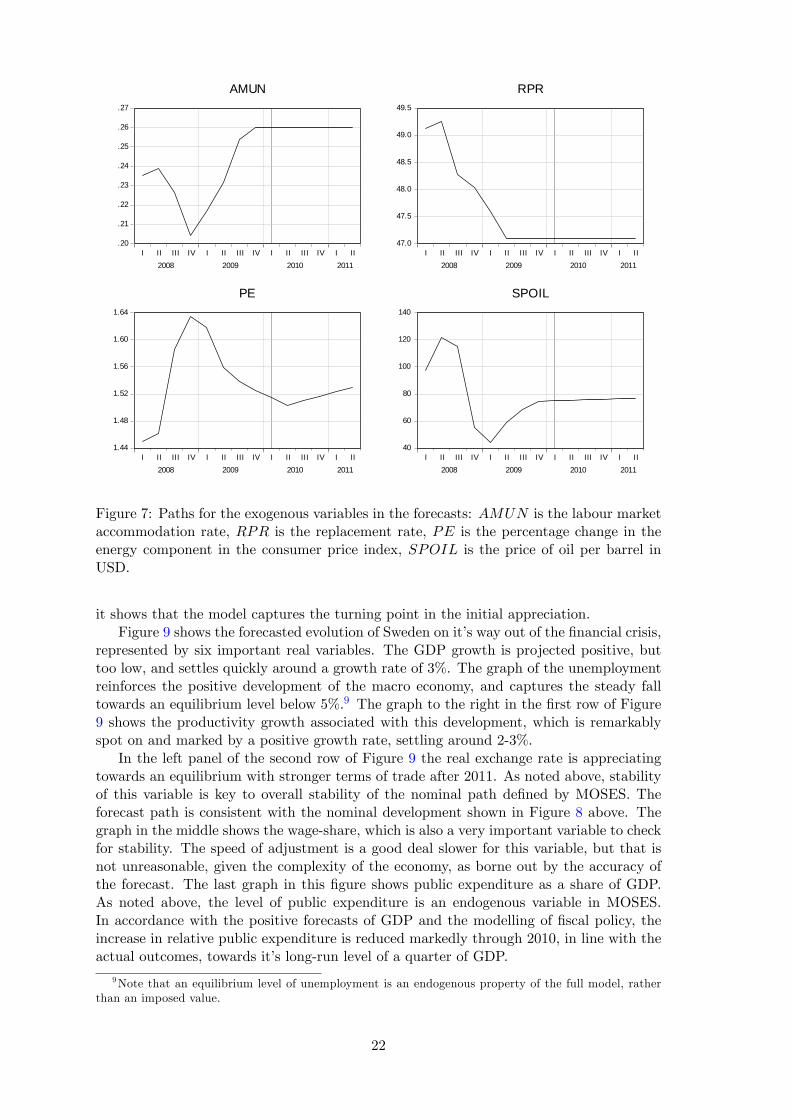


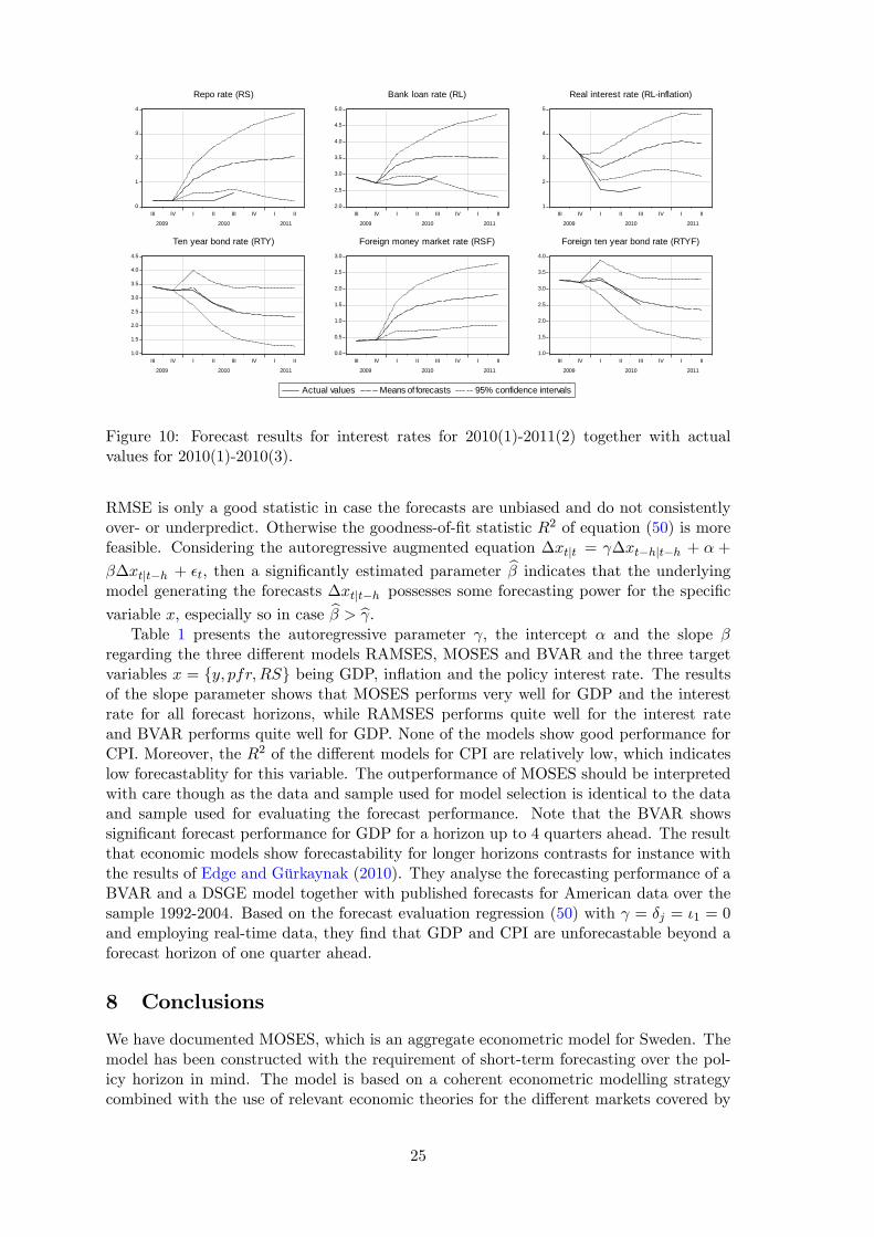

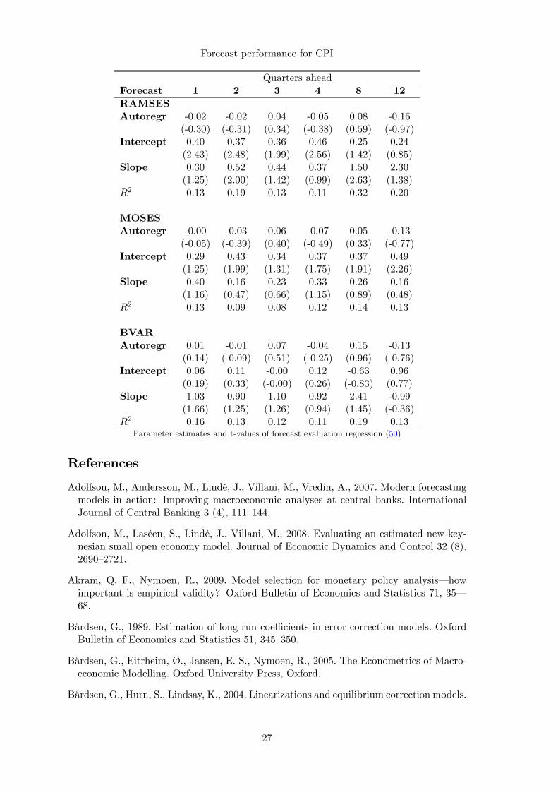


![Moses (Michelangelo) - resources.saylor.org · Moses (Michelangelo) 1 Moses (Michelangelo) Moses Artist Michelangelo Year c. 1513 – 1515[1] Type Marble Dimensions 235 cm (92.5 in)](https://static.documents.pub/doc/80x56/5c4c4f3993f3c308f757d667/moses-michelangelo-moses-michelangelo-1-moses-michelangelo-moses-artist.jpg)


