MOTIVATIONAL NUMERICAL EXAMPLES FOR … · 2016-11-05 · numerical analysis, in the same way that...

MOTIVATIONAL NUMERICAL EXAMPLES FORELECTRICAL/ELECTRONICS ENGINEERS1

GUERRERO-GARCıA Pablo, (SPAIN), SANTOS-PALOMO Angel, (SPAIN)

Abstract. A collection of non-trivial motivational examples is offered to highlight that,in order to design illustrative examples for a whole course on numerical methods like thoseenvisaged for the Education Reform at an undergraduate electrical/electronics engineeringlevel, all we need is to carefully choose those examples from their specific field of knowledgeand to present them in a graphical and sketchy manner. A problem/case based learningis thus encouraged.

Key words and phrases. Applications of mathematics in sciences, Mathematics edu-cation and popularization of mathematics, Numerical methods.

Mathematics Subject Classification. Primary 97D40; Secondary 65C20, 47N40.

Falling parachutists and diving spheres do not absolutely motivate an undergraduate elec-trical/electronics engineer to study a first course on numerical methods. On the other hand,we also have to convince our colleagues for the need to include advanced numerical courses intheir forthcoming postgraduate engineering programs.

The main aim of this contribution is to provide a collection of non-trivial motivationalexamples to design illustrative examples for a whole course on numerical methods at whichproblem/case based learning is encouraged. Our teaching experience during fifteen years withelectrical/electronics engineers revealed that pupils want to know concrete applications of thesubjects they are currently studying, and they are favourably disposed towards the learningwhether they are sufficiently motivated [9]. A carefully chosen schedule of both the examplesfrom their specific field of knowledge and the order in which they are presented allow pupils todiscover the computational tools they need, and now they study these tools knowing beforehandwhat they use for.

1Technical Report MA-06/01, 30 March 2006, http://www.matap.uma.es/investigacion/tr.html. Poster pre-sented by the starred author (to whom correspondence should be addressed) at the 9th International Conferenceon Applied Mathematics, section “New trends in mathematics education”, Bratislava (Slovakia), 2–5 Febr 2010.

739

Motivational numerical examples for electrical/electronics engineers P. Guerrero-García and Á. Santos-Palomo

@ APLIMAT February 2010 ISBN: 978-80-89313-47-1

Unfortunately, to collect a handful of specific examples to illustrate every aspect of a numer-ical course is a tedious task, but the outcomes are highly satisfactory. Apart from several elec-trical/electronics numerical examples that can be found in usual application-oriented textbookson numerical methods, we have adapted some examples from electrical/electronics engineeringtextbooks as those on circuit theory [2], power system analysis [3] and adaptive filter theory[5], as well as from more advanced sources like [10]. This variety of subjects to be coveredimplies that the adaptation is by no means trivial: it has to be done in a graphical and concisemanner, because each example must be explained in no more than twenty-five minutes sincewe do not want to spend more than ten hours in total for the expository lectures throughout athree ECTS-credits course.

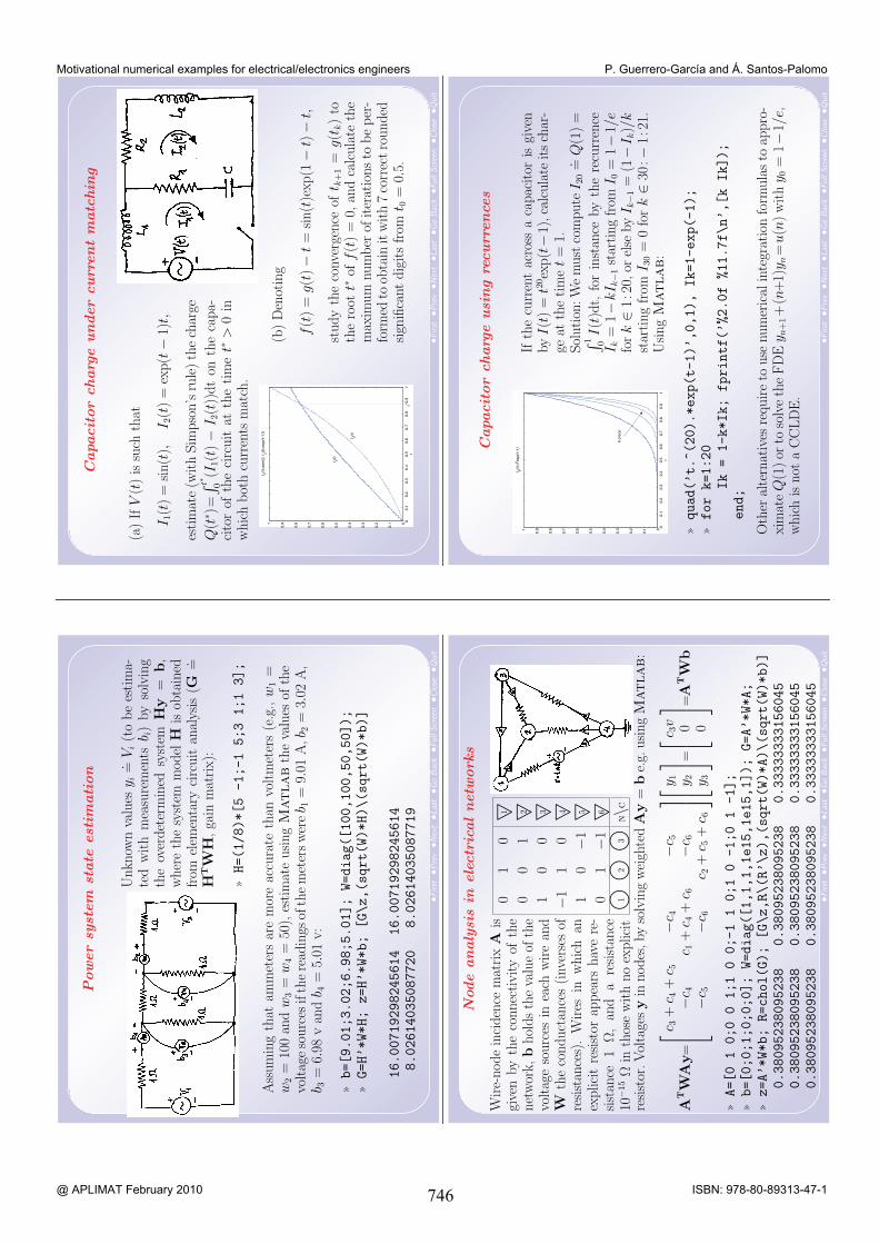
The examples, with suitable references to where have been taken from, can be classifiedas follows: (1) Nonlinear equations and optimization: Potentiometer for energy dissipation [1,§8.3], Impedance in a parallel RLC circuit [1, P8.24], Ebers-Moll equation to model npn tran-sistors [2, §5.1.4], Inductor dimensions to maximize its inductance [1, P16.12], Potentiometer tomaximize power transfer [1, §16.3]. (2) Numerical linear algebra: Loop analysis in an electricalcircuit [6, E2.1], Adaptive filtering of a data sequence [5], Image compression [4, C0.5], Electro-static fields in regions with no free charge [1, §32.3], Transient behaviour of an electrical circuit[1, §28.3]. (3) Interpolation and approximation: Hard-wiring transcendental functions [4, P5.1],Least-squares filtering of signals [4, C0.18], Approximate Fourier series expansions [8, P24.DI],Power system state estimation [3, §15.1], Node analysis in electrical networks [10, §4.2]. (4)Differential problems: Capacitor charge under current matching [7, E10.16], Capacitor chargeusing recurrences [4, P2.1], Serial and parallel RLC circuits [4, E9.1], Transient behaviour ofan electrical circuit [7, E10.16], Particle movement subject to a potential [6, P10.7].

This battery could be helpful for other numerical teachers during their lesson preparationto highlight some specific engineering applications that increase the degree of popularization ofnumerical analysis, in the same way that a magician has her own bouquet of enchanting tricks.In the following six pages you can find our twenty-four cards. Which ones are yours?

References

[1] CHAPRA, S., CANALE, R.: Numerical Methods for Engineers. McGraw-Hill, 3rd ed.,1998.

[2] CHUA, L., DESOER, C., KUH, E.: Linear and Nonlinear Circuits. McGraw-Hill, 1987.[3] GRAINGER, J., STEVENSON, W.: Power System Analysis. McGraw-Hill, 1st ed., 1994.[4] GUERRERO-GARCıA, P.: Slides for a Course on Numerical Methods (Spanish). Dpt.

Applied Mathematics, University of Malaga, December 2003.[5] HAYKIN, S.: Adaptive Filter Theory. Prentice-Hall, 3rd ed., 1996.[6] HEATH, M.: Scientific Computing: An Introductory Survey. McGraw-Hill, 2nd ed., 2002.[7] NAKAMURA, S.: Numerical Analysis and Graphic Visualization with Matlab. Prentice-

Hall, 1st ed., 1996.[8] SANTOS-PALOMO, A.: Slides for a Course on Numerical Methods (Spanish). Dpt. Ap-

plied Mathematics, University of Malaga, September 2001.[9] SCHUNK, D., PINTRICH, P., MEECE, J.: Motivation in Education: Theory, Research,

and Applications. Prentice-Hall, 3rd ed., 2009.[10] VAVASIS, S.: Stable numerical algorithms for equilibrium systems. SIAM J. Matrix Anal.

Appl., 15(4):1108–1131, October 1994.

740



Current address

Pablo Guerrero-Garcıa ([email protected]), Tchng. Fellow Numerical MethodsDepartment of Applied Mathematics, University of Malaga,Complejo Tecnologico (ETSI Telecomunicacion), Campus de Teatinos s/n,29071 Malaga (Spain), Phones: +34 95213 7168/2745.e-mail: [email protected]

Angel Santos-Palomo ([email protected]), Professor on Numerical MethodsDepartment of Applied Mathematics, University of Malaga,Complejo Tecnologico (ETSI Telecomunicacion), Campus de Teatinos s/n,29071 Malaga (Spain), Phones: +34 95213 7168/2745.

741



•First

•Pre

v•N

ext•L

ast•G

oB

ack

•Full

Scr

een

•Clo

se•Q

uit

Pote

ntiom

ete

rfo

renerg

ydis

sipation

Var

iation

ofch

arge

q(c

oulo

mbs)

onth

eca

pac

itor

asa

funct

ion

oftim

e:

q=

q 0·ex

p

( −Rt

2L

) ·cos

⎛ ⎝ t√ 1 LC

−( R 2L

) 2⎞ ⎠(q

/q0

=0.

01,L

=5

H,C

=10

−4F)

Res

ista

nce

Rof

the

pot

entiom

eter

todis

sipat

eth

est

ored

char

gein

t=

0.05

sec

ata

spec

ific

rate

(in

par

ticu

lar,

to1

%of

its

orig

inal

valu

e):

f(R

)=

exp(−

0.00

5·R

)·c

os(0

.05√ 20

00−

0.01

·R2 )−

0.01

=0

Sol

ution

:T

he

resi

stan

ceof

the

pot

entiom

eter

must

be

R≈

328.

1514

Ω

•First

•Pre

v•N

ext•L

ast•G

oB

ack

•Full

Scr

een

•Clo

se•Q

uit

Imped

ance

ina

para

llelR

LC

circuit

(I)

1

Z(ω

)=

√ 1 R2

+

( ωC−

1 ωL

) 2

(R=

225

Ω,C

=6·1

0−5

F,L

=0.

5H

)0

100

200

300

400

050100

150

200

Z(

)

010

020

030

040

0

0123

Z’(

)

(a)

Angu

lar

freq

uen

cyω

that

resu

lts

inan

imped

ance

Z(ω

)of

100

Ω:

f(ω

)=

1√

150

625

+( 0.

0000

6ω−

2) 2−

100

=0

Sol

uti

ons:

ω=

(±50√ 11

345±

250√ 65

)/27

≈(±

122.

5956

)∨(±

271.

8967

)

•First

•Pre

v•N

ext•L

ast•G

oB

ack

•Full

Scr

een

•Clo

se•Q

uit

Ebe

rs-M

oll

equation

tom

odelnpn

transi

stors

Let

E,R

0,V

,I

,I

,α

and

αbe

give

nco

nst

ants

.C

alcu

late

the

curr

ents

Ian

dth

evo

ltag

esV

corr

espon

-din

gto

fixed

valu

esof

ωan

dt

(i.e

.,V

1co

nst

ant)

if,

bes

ides

ofK

irch

off’s

law

(i.e

.,V

2=

−I2·R

(t))

,th

ese

equat

ions

hol

dfo

rx

=[I

1;I 2

;V2]∈

R3 :

I 1=

−I·( ex

p( −

1 T

) −1) +

αI

·( exp( −

2 T

) −1)

I 2=

αI

·( exp( −

1 T

) −1) −

I·( ex

p( −

2 T

) −1)⎫ ⎬ ⎭

f 1(x

)=

I 1+

I( ex

p( −

cos(

)T

) −1) −

αI

( exp( −

2 T

) −1) =

0

f 2(x

)=

I 2−

αI

( exp( −

cos(

)T

) −1) +

I( ex

p( −

2 T

) −1) =

0

f 3(x

)=

I 2R

0sin

(t)+

V2

=0

⎫ ⎪ ⎪ ⎬ ⎪ ⎪ ⎭

•First

•Pre

v•N

ext•L

ast•G

oB

ack

•Full

Scr

een

•Clo

se•Q

uit

Imped

ance

ina

para

llelR

LC

circuit

(II)

1

Z(ω

)=

√ 1 R2

+

( ωC−

1 ωL

) 2

(R=

225

Ω,C

=6·1

0−5

F,L

=0.

5H

)0

100

200

300

400

050100

150

200

Z(

)

010

020

030

040

0

0123

Z’(

)

(b)

Angu

lar

freq

uen

cyto

obta

inth

em

axim

um

imped

ance

:

h(ω

)=

f′ (ω

)=

( 0.00

006ω

−2) ·( 0.

0000

6+

2 2

)√ (

150

625

+( 0.

0000

6ω−

2) 2) 3

=0

Sol

uti

ons:

(±10

0√ 30/3

)∨

(±10

0i√ 30

/3)≈

(±18

2.57

)∨

(±18

2.57

i)

742



•First

•Pre

v•N

ext•L

ast•G

oB

ack

•Full

Scr

een

•Clo

se•Q

uit

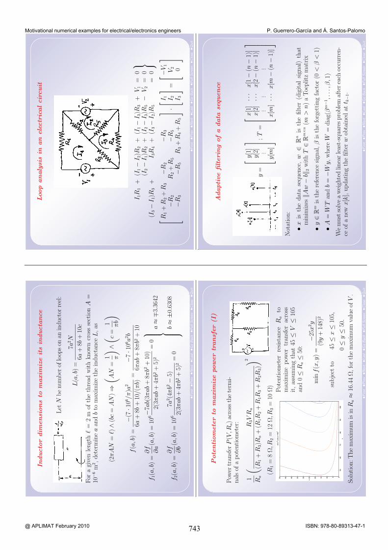
Inducto

rdim

ensi

ons

tom

axim

ize

its

inducta

nce

Let

Nbe

num

ber

oflo

opson

anin

duct

orre

el:

L(a

,b)

=7a

2 N

6a+

8b+

10c

For

agi

ven

lengt

h

=2

mof

the

thre

adw

ith

know

ncr

oss

sect

ion

A=

10−6

m2 ,

det

erm

ine

aan

db

tom

axim

ize

the

induct

ance

L,as

(2πA

N=

)∧

(bc

=A

N)⇒

( AN

=1 π

) ∧( c

=1 πb)

f(a

,b)

=−(

7·1

06 /π)a

2

6a+

8b+

10/(

πb)

=−7

·106 a

2 b

6πab

+8π

b2+

10

f 1(a

,b)

=∂f

∂a

(a,b

)=

106−7

ab(

3πab

+8π

b2+

10)

2(3π

ab

+4π

b2+

5)2

=0

f 2(a

,b)

=∂f ∂b(a

,b)

=10

67a

2 (4π

b2−

5)

2(3π

ab

+4π

b2+

5)2

=0

⎫ ⎪ ⎪ ⎪ ⎪ ⎬ ⎪ ⎪ ⎪ ⎪ ⎭a≈

∓3.3

642

b≈

±0.6

308

•First

•Pre

v•N

ext•L

ast•G

oB

ack

•Full

Scr

een

•Clo

se•Q

uit

Pote

ntiom

ete

rto

maxim

ize

power

transf

er

(I)

Pow

ertr

ansf

erP

(V,R

)ac

ross

the

term

i-nal

sof

apot

enti

omet

er:

1 R

(R

3VR

(R1+

R3)

R+

(R1R

2+

R1R

3+

R2R

3)

) 2(R

1=

8Ω

,R2

=12

Ω,R

3=

10Ω

)

5060

7080

9010

005101520253035404550

x

y

22

Pot

enti

omet

erre

sist

ance

Rto

max

imiz

epow

ertr

ansf

erac

ross

it,as

sum

ing

that

45≤

V≤

105

and

0≤

R≤

50:

mın

f(x

,y)

=−2

5x2 y

(9y

+14

8)2

subje

ctto

45≤

x≤

105,

0≤

y≤

50.

Sol

uti

on:T

he

max

imum

isin

R≈

16.4

4Ω

,fo

rth

em

axim

um

valu

eof

V.

•First

•Pre

v•N

ext•L

ast•G

oB

ack

•Full

Scr

een

•Clo

se•Q

uit

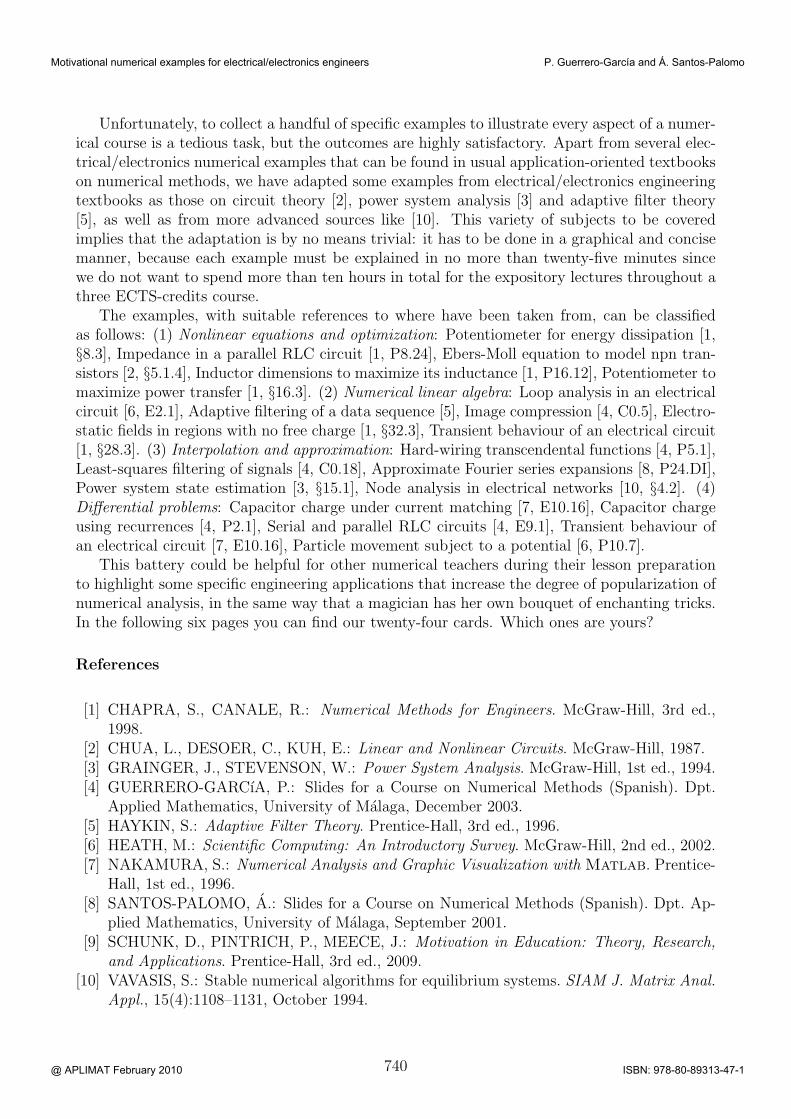
Loop

analy

sis

inan

electr

icalcircuit

I 1R

1+

(I1−

I 2)R

2+

(I1−

I 3)R

3+

V1

=0

(I2−

I 1)R

2+

(I2−

I 3)R

5−

V2

=0

(I3−

I 1)R

3+

I 3R

4+

(I3−

I 2)R

5=

0

⎫ ⎬ ⎭⎡ ⎣R

1+

R2+

R3

−R2

−R3

−R2

R2+

R5

−R5

−R3

−R5

R3+

R4+

R5

⎤ ⎦ ·⎡ ⎣I 1 I 2 I 3

⎤ ⎦ =⎡ ⎣−V

1V

2 0

⎤ ⎦

•First

•Pre

v•N

ext•L

ast•G

oB

ack

•Full

Scr

een

•Clo

se•Q

uit

Adaptive

filterin

gofa

data

sequence

y=

⎡ ⎢ ⎢ ⎣y[1

]y[2

]. . .

y[m

]

⎤ ⎥ ⎥ ⎦;T=

⎡ ⎢ ⎢ ⎣x[1

]···

x[1−

(n−

1)]

x[2

]···

x[2−

(n−

1)]

. . .. . .

. . .x[m

]···

x[m

−(n

−1)

]

⎤ ⎥ ⎥ ⎦N

otat

ion:

•xis

the

dat

ase

quen

ce,

w∈

Ris

the

filte

r(d

igit

alsi

gnal

)th

atm

inim

izes

‖Aw−

b‖2

wit

hT∈

R×

(m>

n)

aToe

plitz

mat

rix

•y∈

Ris

the

refe

rence

sign

al,β

isth

efo

rget

ting

fact

or(0

<β

<1)

•A=

WT

and

b=−W

y,w

her

eW

=dia

g(β

−1,.

..,β

,1)

We

must

solv

ea

wei

ghte

dlinea

rle

ast-

squar

espro

ble

maf

terea

choc

curr

en-

ceof

anew

x[k

],updat

ing

the

filte

rw

obta

ined

att

−1.

743



•First

•Pre

v•N

ext•L

ast•G

oB

ack

•Full

Scr

een

•Clo

se•Q

uit

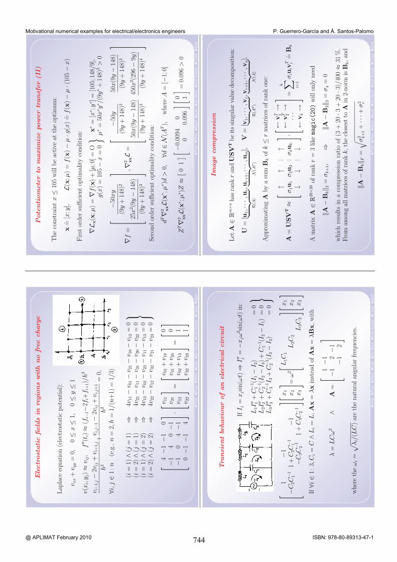
Electr

ost

atic

field

sin

regio

ns

with

no

free

charg

e

Lap

lace

equat

ion

(ele

ctro

stat

icpot

ential

):

v+

v=

0,0≤

x≤

1,0≤

y≤

1

v(x

,y)≈

v,

f′′ (

t)≈

(f−1−2

f+

f+

1)/h

2

v−1

−2v

+v

+1

h2

+v

−1−

2v+

v+

1

h2

=0,

∀i,j

∈1:n

(e.g

.,n

=2,

h=

1/(n

+1)

=1/

3)

(i=

1)∧

(j=

1)⇒

4v11−

v 01−

v 21−

v 10−

v 12

=0

(i=

2)∧

(j=

1)⇒

4v21−

v 11−

v 31−

v 20−

v 22

=0

(i=

1)∧

(j=

2)⇒

4v12−

v 02−

v 22−

v 11−

v 13

=0

(i=

2)∧

(j=

2)⇒

4v22−

v 12−

v 32−

v 21−

v 23

=0

⎫ ⎪ ⎬ ⎪ ⎭⎡ ⎢ ⎣

4−1

−10

−14

0−1

−10

4−1

0−1

−14

⎤ ⎥ ⎦·⎡ ⎢ ⎣v 11

v 21

v 12

v 22

⎤ ⎥ ⎦=⎡ ⎢ ⎣v 0

1+

v 10

v 31+

v 20

v 02+

v 13

v 32+

v 23

⎤ ⎥ ⎦=⎡ ⎢ ⎣0 0 1 1

⎤ ⎥ ⎦

•First

•Pre

v•N

ext•L

ast•G

oB

ack

•Full

Scr

een

•Clo

se•Q

uit

Tra

nsi

entbe

havio

ur

ofan

electr

icalcircuit

IfI

=x

sin(ω

t)⇒

I′′

=−x

ω2 s

in(ω

t)in

:

L1I

′′ 1+

C−1 1

(I1−

I 2)

=0

L2I

′′ 2+

C−1 2

(I2−

I 3)+

C−1 1

(I2−

I 1)

=0

L3I

′′ 3+

C−1 3

I 3+

C−1 2

(I3−

I 2)

=0

⎫ ⎬ ⎭⎡ ⎣

1−1

−C2C

−1 11

+C

2C−1 1

−1−C

3C−1 2

1+

C3C

−1 2

⎤ ⎦⎡ ⎣x1

x2

x3

⎤ ⎦ =ω2⎡ ⎣L

1C1

L2C

2L

3C3

⎤ ⎦⎡ ⎣x1

x2

x3

⎤ ⎦If∀i

∈1:3,

C=

C∧

L=

L,A

x=

λx

inst

ead

ofA

x=

λB

x,w

ith

λ=

LC

ω2

∧A

=

⎡ ⎣1

−1−1

2−1

−12

⎤ ⎦w

her

eth

eω

=√ λ

/(L

C)

are

the

nat

ura

lan

gula

rfr

equen

cies

.

•First

•Pre

v•N

ext•L

ast•G

oB

ack

•Full

Scr

een

•Clo

se•Q

uit

Pote

ntiom

ete

rto

maxim

ize

power

transf

er

(II)

The

const

rain

tx≤

105

willbe

active

atth

eop

tim

um

:

x. =

[x;y

],L(

x;μ

)=

f(x

)−

μ·g

(x)

. =f(x

)−

μ·(1

05−

x)

First

order

suffi

cien

top

tim

ality

conditio

n:

∇Lx(x

;μ)

=∇f

(x)+

[μ;0

]=

Og(x

)=

105−

x=

0

x∗

=[x

∗ ;y∗ ]

=[1

05;1

48/9

],μ∗

=50

x∗ y

∗ /(9

y∗+

148)

2>

0

∇f=

⎡ ⎢ ⎢ ⎢ ⎣−5

0xy

(9y

+14

8)2

25x

2 (9y

−14

8)

(9y

+14

8)3

⎤ ⎥ ⎥ ⎥ ⎦,∇2 xxL

=

⎡ ⎢ ⎢ ⎢ ⎣−5

0y

(9y

+14

8)2

50x(9

y−

148)

(9y

+14

8)3

50x(9

y−

148)

(9y

+14

8)3

450x

2 (29

6−

9y)

(9y

+14

8)4

⎤ ⎥ ⎥ ⎥ ⎦Sec

ond

order

suffi

cien

top

tim

ality

conditio

n:

d∇2 x

xL(

x∗ ;

μ∗ )

d>

0,∀d

∈N

(A),

wher

eA

=[−

1;0]

Z∇2 x

xL(

x∗ ;

μ∗ )

Z≈

[ 01][ −0

.009

40

00.

096

][ 0 1

] =0.

096

>0

•First

•Pre

v•N

ext•L

ast•G

oB

ack

•Full

Scr

een

•Clo

se•Q

uit

Image

com

pre

ssio

n

Let

A∈

R×

has

rank

ran

dU

SV

Tbe

itssi

ngu

larva

lue

dec

ompos

itio

n:

U=

[u1,···,

u︸

︷︷︸

R()

,u+

1,···,

u︸

︷︷︸

N(

T)

],V

=[v

1,···,

v︸

︷︷︸

R(T)

,v+

1,···,

v︸

︷︷︸

N(

)

].

Appro

xim

atin

gA

bya

sum

Bof

k≤

rm

atri

ces

ofra

nk

one:

A=

USV

T≈

⎡ ⎣↑↑

. . .↑

σ1u

1σ

2u2

. . .σ

u↓

↓. . .

↓

⎤ ⎦ ·⎡ ⎢ ⎣←v

1→

←v

2→

···

←v

→

⎤ ⎥ ⎦=∑ =

1

σu

v. =

B

Am

atri

xA

∈R

20×2

0of

rank

r=

3lik

emagic(20)

willon

lynee

d

‖A−

B‖ 2

=σ

+1,

⇒‖A

−B

3‖ 2=

σ4

=0

whic

hre

sult

sin

aco

mpre

ssio

nra

tio

of(3

+20

·3+

20·3

)/40

0≈

31%

.Fro

mam

ong

allm

atri

ces

ofra

nk

k,th

ecl

oses

tto

Ain

2-nor

mis

B,an

d

‖A−

B‖

=√ σ

2 +1+···+

σ2

744



•First

•Pre

v•N

ext•L

ast•G

oB

ack

•Full

Scr

een

•Clo

se•Q

uit

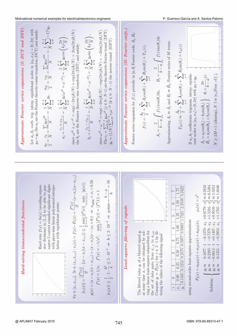
Hard

-wir

ing

transc

endenta

lfu

nctions

11.

11.

21.

31.

41.

51.

61.

71.

81.

92

0

0.1

0.2

0.3

0.4

0.5

0.6

0.7

Har

d-w

ire

f(x

)=

ln(x

)(a

void

ing

expen

-si

vediv

isio

ns)

in[1

,2]to

be

able

togu

a-ra

ntee

5co

rrec

tro

unded

sign

ifica

ntdig

its

with

pie

ce-w

ise

linea

rpol

ynom

iali

nter

po-

lation

with

equid

ista

ntpoi

nts.

∀x∈

[x,x

+1],∃c

∈(x

,x+

1):e 1

(x)

=f(x

)−P

1(x)

=f′′ (

c)

2!·(x

−x)(

x−x

+1)

|e 1(x

)|=

|f′′ (

c)|

2!·|(

x−

x)(

x−

x+

1)|≤

1 2m

ax1

2|f′

′ (c)|

max

i≤≤

i+1

|g(x)|,

g(x

)=

(x−

x)(

x−

x+

1)=

(x−

x)(

x−

(x+

h))

⇒xm

in=

x+

0.5h

f′ (x)

=1/

x,

f′′ (

x)

=−1

/x2 ,

max

12|f′

′ (c)|=

|f′′ (1)|=

1

|e 1(x

)|≤

1 2·1

·h2 4≤

5·1

0−5⇒

h≤

2·1

0−2⇒

poi

nts

=b−

a

h=

50

•First

•Pre

v•N

ext•L

ast•G

oB

ack

•Full

Scr

een

•Clo

se•Q

uit

Lea

st-s

quare

sfilteri

ng

ofsi

gnals

The

filte

red

valu

eg

ofa

blu

rred

sign

aly

atso

me

tim

ex

can

be

obta

ined

byso

l-vi

ng

alinea

rle

ast-

squar

essu

bpro

ble

mfo

rth

ese

tof

dat

apai

rsfr

omx

−2to

x+

2.C

ompute

g=

P2(

x)

for

i∈

2:5

byfil

-te

ring

the

valu

esof

the

follow

ing

sign

al

00.

20.

40.

60.

81

1.2

1.4

1.6

1.8

0

0.51

1.52

2.53

3.5

r0

12

34

56

7x

0.00

0.25

0.50

0.75

1.00

1.25

1.50

1.75

y0.

1165

0.12

520.

2575

0.59

770.

9303

1.73

212.

2559

3.24

22

usi

ng

seco

nd-o

rder

leas

t-sq

uar

esap

pro

xim

atio

ns

P2(

x)

=a

0ϕ0(

x)+

a1ϕ

1(x)+

a2ϕ

2(x),

ϕ(x

)=

x

Sol

uti

on:

⎧ ⎪ ⎨ ⎪ ⎩g 2≈

0.10

77·1

−0.1

379·x

2+

0.97

79·x

2 2≈

0.28

32g 3

≈0.

2283

·1−0

.727

8·x

3+

1.52

16·x

2 3≈

0.53

84g 4

≈−0

.061

4·1

+0.

1407

·x4

+0.

9559

·x2 4≈

1.03

52g 5

≈0.

1355

·1−0

.295

3·x

5+

1.17

65·x

2 5≈

1.60

46

•First

•Pre

v•N

ext•L

ast•G

oB

ack

•Full

Scr

een

•Clo

se•Q

uit

Appro

xim

ate

Fouri

er

serie

sexpansi

ons

(I:D

CT

and

DST)

Let

a,b

coef

s.tr

ig.

inte

rp.

equid

ista

ntnod

esin

[x0,

x]=

[0,2

π]

with

y=

y 0;t

hea

are

the

Fou

rier

dis

cret

eco

sine

tran

sfor

m(D

CT

)an

dsa

tisf

y:

a0 2

=c 0 N

=

∑ yω

0

N=

1 N

−1 ∑ =0

y,

a 2=

c N=

∑ yω

N=

1 N

−1 ∑ =0

(−1)

y,

a=

c+

c−

N=

1 N

−1 ∑ =0

y(ω

+ω

−)

=2 N

−1 ∑ =0

yco

s

( kj2π N

) ,

since

ω+

ω−

=ex

p(−

2πij

k/N

)+

exp(2

πij

k/N

)=

2cos

(2πjk

/N);

the

bar

eth

eFou

rier

dis

cret

esi

ne

tran

sfor

m(D

ST

)an

dsa

tisf

y:

b=

ic−

c−

N=

i N

−1 ∑ =0

y(ω

−ω

−)

=2 N

−1 ∑ =0

ysi

n

( kj2π N

) ,

since

ω−

ω−

=ex

p(−

2πij

k/N

)−ex

p(2

πij

k/N

)=−2

isin

(2πjk

/N).

Thec

=∑ −

1=

0y

ω(j

∈0:N−1

)ar

eth

edis

cret

eFou

rier

tran

sf.(

DFT

),

y=

(1/N

)∑ −

1=

0c

ω−

(k∈

0:N−1

)th

ein

vers

etr

ansf

.(I

DFT

).

•First

•Pre

v•N

ext•L

ast•G

oB

ack

•Full

Scr

een

•Clo

se•Q

uit

Appro

xim

ate

Fourie

rse

rie

sexpansi

ons

(II:

Fourie

rco

efs

.)

Fou

rier

seri

esex

pan

sion

forf(z

)per

iodic

in[a

,b]Fou

rier

coef

s.A

,B:

f(z

)=

A0 2

+

∞ ∑ =1

Aco

s(θ

)+

∞ ∑ =1

Bsi

n(θ

). =

T∞

(z),

A=

2

b−

a

∫ f(z

)cos

(θ)d

z,B

=2

b−

a

∫ f(z

)sin

(θ)d

z

Appro

xim

atin

gA

≈A

and

B≈

B,Fou

rier

seri

esof

Mte

rms:

T(z

)≈

A0 2

+∑ =

1

Aco

s(θ

)+

∑ =1

Bsi

n(θ

). =

t(z

)

Ifa

,bco

effici

ents

trig

onom

.in

terp

.eq

uid

is-

tant

nod

esin

[x0,

x]=

[0,2

π]w

ith

y=

y 0:

A=

aco

s(θ

)−

bsi

n(θ

)

B=

asi

n(θ

)+

bco

s(θ

)

θ

=2π

b−

ajz

N≥

2M+

1(a

lias

ing)

,N↑⇒

|e(F

our.

cf)|↓

02

46

0

0.2

0.4

0.6

0.81

1.2

745



•First

•Pre

v•N

ext•L

ast•G

oB

ack

•Full

Scr

een

•Clo

se•Q

uit

Power

syst

em

state

est

imation

Unkn

own

valu

esy

. =V

(to

be

estim

a-te

dw

ith

mea

sure

men

tsb

)by

solv

ing

the

over

det

erm

ined

syst

emH

y=

b,

wher

eth

esy

stem

mod

elH

isob

tain

edfr

omel

emen

tary

circ

uit

anal

ysis

(G. =

HTW

H,ga

inm

atrix)

:

H=(1/8)*[5

-1;-1

5;3

1;1

3];

Ass

um

ing

that

amm

eter

sar

em

ore

accu

rate

than

voltm

eter

s(e

.g.,

w1

=w

2=

100

and

w3

=w

4=

50),

estim

ate

usi

ng

Matlab

the

valu

esof

the

voltag

eso

urc

esif

the

read

ings

ofth

em

eter

sw

ereb 1

=9.

01A

,b2

=3.

02A

,b 3

=6.

98v

and

b 4=

5.01

v:

b=[9.01;3.02;6.98;5.01];

W=diag([100,100,50,50]);

G=H’*W*H;

z=H’*W*b;

[G\z,(sqrt(W)*H)\(sqrt(W)*b)]

16.00719298245614

16.00719298245614

8.02614035087720

8.02614035087719

•First

•Pre

v•N

ext•L

ast•G

oB

ack

•Full

Scr

een

•Clo

se•Q

uit

Node

analy

sis

inelectr

icalnetw

ork

s

Wir

e-nod

ein

ciden

cem

atri

xA

isgi

ven

byth

eco

nnec

tivi

tyof

the

net

wor

k,b

hol

ds

the

valu

eof

the

volt

age

sourc

esin

each

wir

ean

dW

the

conduct

ance

s(i

nver

ses

ofre

sist

ance

s).

Wir

esin

whic

han

explici

tre

sist

orap

pea

rshav

ere

-si

stan

ce1

Ω,

and

are

sist

ance

10−1

5Ω

inth

ose

wit

hno

explici

t

01

01

00

12

10

03

−11

04

10

−15

01

−16

©1©2

©3N\C

resi

stor

.Vol

tage

sy

innod

es,b

yso

lvin

gw

eigh

ted

Ay

=b

e.g.

usi

ngM

atlab:

ATW

Ay=

⎡ ⎣c 3+

c 4+

c 5−c

4−c

5−c

4c 1

+c 4

+c 6

−c6

−c5

−c6

c 2+

c 5+

c 6

⎤ ⎦⎡ ⎣y 1 y 2 y 3

⎤ ⎦ =⎡ ⎣c 3v 0 0

⎤ ⎦ =ATW

b

A=[0

10;0

01;1

00;-1

10;1

0-1;0

1-1];

b=[0;0;1;0;0;0];

W=diag([1,1,1,1e15,1e15,1]);

G=A’*W*A;

z=A’*W*b;

R=chol(G);

[G\z,R\(R’\z),(sqrt(W)*A)\(sqrt(W)*b)]

0.38095238095238

0.38095238095238

0.33333333156045

0.38095238095238

0.38095238095238

0.33333333156045

0.38095238095238

0.38095238095238

0.33333333156045

•First

•Pre

v•N

ext•L

ast•G

oB

ack

•Full

Scr

een

•Clo

se•Q

uit

Capacitor

charg

eunder

curre

ntm

atc

hin

g

(a)

IfV

(t)

issu

chth

at

I 1(t

)=

sin(t

),I 2

(t)

=ex

p(t−

1)t,

estim

ate

(with

Sim

pso

n’s

rule

)th

ech

arge

Q(t

∗ )=∫ ∗ 0

(I1(

t)−

I 2(t

))dt

onth

eca

pa-

cito

rof

the

circ

uit

atth

etim

et∗

>0

inw

hic

hbot

hcu

rren

tsm

atch

.

00.

10.

20.

30.

40.

50.

60.

70.

80.

91

0

0.1

0.2

0.3

0.4

0.5

0.6

0.7

0.8

0.91

t

I 1(t)=

sen(

t), I

2

t*

I 1(t)

I 2(t)

(b)

Den

otin

g

f(t

)=

g(t

)−

t=

sin(t

)exp

(1−

t)−

t,

study

the

conv

erge

nce

oft

+1

=g(t

)to

the

root

t∗of

f(t

)=

0,an

dca

lcula

teth

em

axim

um

num

ber

ofiter

atio

ns

tobe

per

-fo

rmed

toob

tain

itw

ith

7co

rrec

tro

unded

sign

ifica

ntdig

its

from

t 0=

0.5.

•First

•Pre

v•N

ext•L

ast•G

oB

ack

•Full

Scr

een

•Clo

se•Q

uit

Capacitor

charg

eusi

ng

recurre

nce

s

00.

10.

20.

30.

40.

50.

60.

70.

80.

91

0

0.1

0.2

0.3

0.4

0.5

0.6

0.7

0.8

0.91

t

I k(t)=

tk

k cr

ece

Ifth

ecu

rren

tac

ross

aca

pac

itor

isgi

ven

byI(t

)=

t20ex

p(t−

1),c

alcu

late

its

char

-ge

atth

eti

me

t=

1.Sol

uti

on:W

em

ust

com

pute

I 20

. =Q

(1)

=∫ 1 0

I(t

)dt,

for

inst

ance

byth

ere

curr

ence

I=

1−

kI

−1st

arti

ng

from

I 0=

1−

1/e

fork∈

1:2

0,or

else

byI

−1=

(1−

I)/

kst

arti

ng

from

I 30

=0

fork∈

30:−

1:2

1.U

sing

Matlab:

quad(’t.^(20).*exp(t-1)’,0,1),

Ik=1-exp(-1);

for

k=1:20

Ik

=1-k*Ik;

fprintf(’%2.0f

%11.7f\n’,[k

Ik]);

end;

Oth

eral

tern

ativ

esre

quir

eto

use

num

eric

alin

tegr

atio

nfo

rmula

sto

appro

-xi

mat

eQ

(1)or

toso

lve

the

FD

Ey

+1+

(n+

1)y

=u(n

)w

ith

y 0=

1−

1/e,

whic

his

not

aC

CLD

E.

746



•First

•Pre

v•N

ext•L

ast•G

oB

ack

•Full

Scr

een

•Clo

se•Q

uit

Seri

aland

para

llelR

LC

circuits

V(t

)=

RI

(t),

V(t

)=

LI′ (

t),

V(t

)=

C−1∫ I

(t)d

t

I(t

)=

R−1

V(t

),I

(t)

=L

−1∫ V(t

)dt,

I(t

)=

CV

′ (t)

I(t

)=

I(t

)+

I(t

)+

I(t

)V

(t)

=V

(t)+

V(t

)+

V(t

)

First

-ord

erO

DE

forI(t

)if

par

alle

lR

LC

circ

uit:

I(t

)=

R−1

V(t

)+L

−1∫ V(t

)dt+

CV

′ (t)⇒

I′ (t)

=

((

))︷

︸︸︷

R−1

V′ (t)

+L

−1V

(t)+

CV

′′ (t)

Sec

ond-o

rder

OD

Efo

rI(t

)if

serial

RLC

circ

uit:

V′ (t)

=R

I′ (t)

+LI′′ (

t)+

C−1

I(t

)⇒

I′′ (

t)=

((

)′ (

))︷

︸︸︷

L−1

V′ (t)−

RL

−1I′ (t)−

L−1

C−1

I(t

)

First

-ord

erO

DE

forI(t

)if

serial

RL

circ

uit

(I(0

)=

0):

V(t

)=

RI(t

)+

LI′ (t)⇒

I′ (t)

=L

−1V

(t)−

RL

−1I(t

)=

f(t

,I(t

))

•First

•Pre

v•N

ext•L

ast•G

oB

ack

•Full

Scr

een

•Clo

se•Q

uit

Tra

nsi

entbe

havio

ur

ofan

electr

icalcircuit

Cir

cuit

com

pon

ents

tost

udy

fort∈

[0,1

]se

c:

V(t

)=

cos(

t),C

=0.

002

F,

L1

=0.

01H

,L2

=0.

5H

,R1

=20

0Ω

,

R2

=20

Ω,I

1(0)

=I 2

(0)

=0

A,Q

(0)

=0

C

Mod

elas

syst

emof

OD

Es

(open

swit

chat

star

t,unch

arge

dca

pac

itor

):

00.

20.

40.

60.

81

0

0.01

0.02

0.03

0.04

0.05

0.06

00.

20.

40.

60.

81

0

0.51

1.5

x 10

I 1(t)

I 2(t)

Q(t

)

⎧ ⎨ ⎩L1I

′ 1+

R1(

I 1−

I 2)+

C−1

Q=

VL

2I′ 2+

R1(

I 2−

I 1)+

R2I

2−

C−1

Q=

0Q

′ =I 1−

I 2⎧ ⎪ ⎪ ⎪ ⎪ ⎨ ⎪ ⎪ ⎪ ⎪ ⎩I

′ 1=

L−1 1

V+

R1L

−1 1(I

2−

I 1)−

L−1 1

C−1

Q︸

︷︷︸

1(

[1;

2;

])

I′ 2=

R1L

−1 2(I

1−

I 2)−

R2L

−1 2I 2

+L

−1 2C

−1Q

︸︷︷

︸2(

[1;

2;

])

Q′ =

I 1−

I 2=

f 3(t

,[I 1

;I2;

Q])

•First

•Pre

v•N

ext•L

ast•G

oB

ack

•Full

Scr

een

•Clo

se•Q

uit

Part

icle

movem

entsu

bje

ctto

apote

ntial(I

)

Sch

rodin

ger

equat

ion

inon

edim

ensi

onfo

rw

ave

funct

ion

ψ(x

):

−ψ′′ (

x)+

V(x

)ψ(x

)=

E·ψ

(x),

ψ(a

)=

0,ψ

(b)

=0,

a≤

x≤

b

Giv

enpot

ential

V(x

)as

afu

nct

ion

ofpar

ticl

epos

itio

n(e

.g.,

V(x

)=

400

with

x∈

[0,1

],V

(x)

=2x

−2w

ith

x∈

[2,3

],..

.),w

ehav

eto

det

erm

ine

the

only

ener

gyle

vels

Eper

mitte

dan

dits

corr

espon

din

gw

ave

funct

ions

ψ(x

),si

nce

|ψ(x

)|2gi

ves

pro

bab

ility

ofpar

ticl

eat

pos

itio

nx.

(a)

Dis

cret

izat

ion

Ay

=h

2 Ey

cont

inuou

spro

ble

mby

finite

diff

eren

ces:

solu

tion

eige

nval

ues

λan

dei

genv

ecto

rsy

() ,

appro

xim

atio

ns

toei

genv

a-lu

esE

≈λ

/h2

and

eige

nfu

nct

ionsψ

(x)

dis

cret

ized

with

step

-siz

eh.

22.

12.

22.

32.

42.

52.

62.

72.

82.

93

0

0.2

0.4

0.6

0.81

h=

0.01

E1≈

10.2

E2≈

39.8

E3≈

89.1

22.

12.

22.

32.

42.

52.

62.

72.

82.

93

0

0.00

5

0.01

0.01

5

0.02

0.02

5

0.03

0.03

5

0.04

0.04

5

0.05

t

2

•First

•Pre

v•N

ext•L

ast•G

oB

ack

•Full

Scr

een

•Clo

se•Q

uit

Particle

movem

entsu

bje

ctto

apote

ntial(I

I)

Sch

rodin

ger

equat

ion

inon

edim

ensi

onfo

rw

ave

funct

ion

ψ(x

):

−ψ′′ (

x)+

V(x

)ψ(x

)=

E·ψ

(x),

ψ(a

)=

0,ψ

(b)

=0,

a≤

x≤

b

Giv

enpot

enti

alV

(x)

asa

funct

ion

ofpar

ticl

epos

itio

n(e

.g.,

V(x

)=

400

wit

hx∈

[0,1

],V

(x)

=2x

−2w

ith

x∈

[2,3

],..

.),w

ehav

eto

det

erm

ine

the

only

ener

gyle

vels

Eper

mit

ted

and

its

corr

espon

din

gw

ave

funct

ions

ψ(x

),si

nce

|ψ(x

)|2gi

ves

pro

bab

ility

ofpar

ticl

eat

pos

itio

nx.

(b)E

igen

valu

esan

dei

genfu

nct

ionsto

appro

xim

ate

the

solu

tion

ofth

eB

VP

−ψ′′ (

x)+

V(x

)ψ(x

)=

f(x

),ψ

(a)

=0,

ψ(b

)=

0,a≤

x≤

b

byth

esp

ectr

alei

genfu

nct

ion

expan

sion

ofa

give

nf(x

)(e

.g.,

f(x

)=

−400

cos2 (

πx)−

2π2 c

os(2

πx)

with

x∈

[0,1

],f(x

)=

x−1

wit

hx∈

[2,3

])

ψ(x

)≈

∑ =1

〈f,ψ

〉E

〈ψ,ψ

〉·ψ

(x)

wher

e〈f

,g〉=

∫ w(x

)f(x

)g(x

)dx,

suit

able

sym

met

riza

tion

fact

orw

(x).

747



748



This pa

ge is

inten

tiona

lly le

ft blan

k

EJEMPLOS NUMERICOS DE MOTIVACION SOBRESISTEMAS ELECTRONICOS DE TELECOMUNICACION1

GUERRERO-GARCıA Pablo?, (Espana), SANTOS-PALOMO Angel, (Espana)

Resumen. Se ofrece una coleccion de ejemplos de motivacion no triviales para enfatizarque, para disenar ejemplos ilustrativos para un curso completo de metodos numericoscomo los que se preveen tras la Reforma Educativa a un nivel de grado para ingenieros ensistemas electronicos de telecomunicacion, todo lo que se necesita es elegir cuidadosamentedichos ejemplos de su campo especıfico de conocimiento y presentarlos de forma grafica yesquematica. Ası estaremos favoreciendo un aprendizaje basado en problemas/casos.

Palabras y frases clave. Aplicaciones matematicas en las ciencias, Didactica matematicay popularizacion de las matematicas, Metodos numericos.Mathematics Subject Classification. Primary 97D40; Secondary 65C20, 47N40.

Los paracaidistas que caen y las esferas que se sumergen no motivan en absoluto a unfuturo ingeniero de sistemas electronicos de telecomunicacion para estudiar un primer cursosobre metodos numericos. Por otra parte, tambien tenemos que convencer a nuestros colegasde la necesidad de incluir cursos numericos avanzados en los venideros programas ingenierilesde postgrado.

El objetivo principal de esta contribucion es proporcionar una coleccion de ejemplos demotivacion no triviales para disenar ejemplos ilustrativos para un curso completo de metodosnumericos en el cual se favorezca el aprendizaje basado en problemas/casos. Nuestra experien-cia docente durante quince anos con ingenieros en sistemas electronicos de telecomunicacionponıa de manifiesto que los alumnos quieren conocer aplicaciones concretas de los temas queestan actualmente estudiando, y que ellos estan predispuestos favorablemente al aprendizaje siestan suficientemente motivados [9]. Una planificacion cuidadosamente seleccionada tanto delos ejemplos de su campo especıfico de conocimiento como del orden en el que dichos ejemplosse presentan permite a los alumnos descubrir las herramientas computacionales que necesitan,y ahora ellos estudian estas herramientas sabiendo de antemano para que las van a usar.

Desgraciadamente, el compendiar un ramillete de ejemplos especıficos que ilustren todoslos aspectos de un curso numerico es una tarea tediosa, pero los resultados son altamentesatisfactorios. Ademas de algunos ejemplos numericos del campo de los sistemas electronicosde telecomunicacion que pueden encontrarse en los habituales libros de texto sobre metodos

1Informe Tecnico MA-06/01, 30 Marzo 2006, http://www.matap.uma.es/investigacion/tr.html. Poster pre-sentado por el autor con asterisco (a quien debe dirigirse la correspondencia) en 9th International Conference onApplied Mathematics, seccion “New trends in mathematics education”, Bratislava (Eslovaquia), 2–5 Febr 2010.

739

Ejemplos numéricos de motivación sobre sistemas electrónicos de telecomunicación P. Guerrero-García y Á. Santos-Palomo


numericos con enfasis en las aplicaciones, hemos adaptado varios ejemplos de los libros de textoingenieriles sobre sistemas electronicos de telecomunicacion como los de teorıa de circuitos [2],analisis de sistemas de potencia [3] y teorıa de filtros adaptativos [5], ası como de fuentes masavanzadas como [10]. Esta variedad de aspectos a contemplar implica que la adaptacion no esen absoluto trivial: tiene que hacerse de una manera grafica y concisa, porque cada ejemplodebe explicarse como maximo en veinticinco minutos dado que no queremos dedicar mas dediez horas en total para las clases expositivas a lo largo de un curso de tres creditos ECTS.

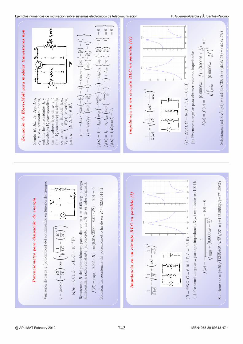
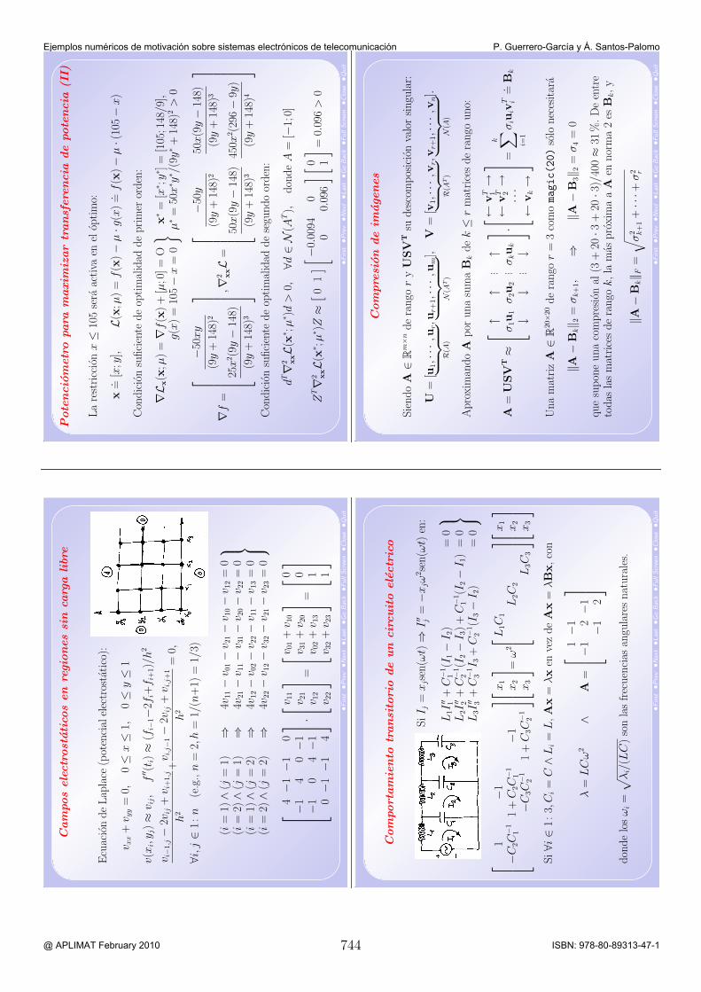
Los ejemplos, con adecuadas referencias a donde los hemos sacado, pueden clasificarse comosigue: (1) Ecuaciones no lineales y optimizacion: Potenciometro para disipacion de energıa [1,§8.3], Impedancia en un circuito RLC en paralelo [1, P8.24], Ecuacion de Ebers-Moll paramodelar transistores npn [2, §5.1.4], Dimensionado de bobina para maximizar su inductancia[1, P16.12], Potenciometro para maximizar transferencia de potencia [1, §16.3]. (2) Algebralineal numerica: Analisis de mallas en un circuito electrico [6, E2.1], Filtrado adaptativo de unasecuencia de datos [5], Compresion de imagenes [4, C0.5], Campos electrostaticos en regionessin carga libre [1, §32.3], Comportamiento transitorio de un circuito electrico [1, §28.3]. (3)Interpolacion y aproximacion: Cableado de funciones trascendentes [4, P5.1], Filtrado mınimo-cuadratico de senales [4, C0.18], Desarrollos aproximados de Fourier [8, P24.DI], Estimacion deestado de sistemas de potencia [3, §15.1], Analisis de nodos en redes electricas [10, §4.2]. (4)Problemas diferenciales: Carga de condensador bajo coincidencia de intensidades [7, E10.16],Carga de condensador usando recurrencias [4, P2.1], Circuitos RLC serie y paralelo [4, E9.1],Comportamiento transitorio de un circuito electrico [7, E10.16], Movimiento de partıcula sujetaa potencial [6, P10.7].

Esta baterıa de ejemplos podrıa ser de utilidad para otros profesores numericos durantela preparacion de sus clases para enfatizar algunas aplicaciones ingenieriles especıficas queaumenten el grado de popularidad del analisis numerico, de la misma forma que un magodispone de su propio abanico de trucos de magia. En las seis paginas siguientes puedes encontrarnuestros veinticuatro naipes. ¿Cuales son los tuyos?

Referencias

[1] CHAPRA, S., CANALE, R.: Numerical Methods for Engineers. McGraw-Hill, 3rd ed.,1998.

[2] CHUA, L., DESOER, C., KUH, E.: Linear and Nonlinear Circuits. McGraw-Hill, 1987.[3] GRAINGER, J., STEVENSON, W.: Power System Analysis. McGraw-Hill, 1st ed., 1994.[4] GUERRERO-GARCıA, P.: Slides for a Course on Numerical Methods (Spanish). Dpt.

Applied Mathematics, University of Malaga, December 2003.[5] HAYKIN, S.: Adaptive Filter Theory. Prentice-Hall, 3rd ed., 1996.[6] HEATH, M.: Scientific Computing: An Introductory Survey. McGraw-Hill, 2nd ed., 2002.[7] NAKAMURA, S.: Numerical Analysis and Graphic Visualization with Matlab. Prentice-

Hall, 1st ed., 1996.[8] SANTOS-PALOMO, A.: Slides for a Course on Numerical Methods (Spanish). Dpt. Ap-

plied Mathematics, University of Malaga, September 2001.[9] SCHUNK, D., PINTRICH, P., MEECE, J.: Motivation in Education: Theory, Research,

and Applications. Prentice-Hall, 3rd ed., 2009.[10] VAVASIS, S.: Stable numerical algorithms for equilibrium systems. SIAM J. Matrix Anal.

Appl., 15(4):1108–1131, October 1994.

740



Direcciones actuales

Pablo Guerrero-Garcıa ([email protected]), Asociado (TC) Metodos Numericos

Departamento de Matematica Aplicada, Universidad de Malaga,Complejo Tecnologico (ETSI Telecomunicacion), Campus de Teatinos s/n,29071 Malaga (Espana), Telefono +34 95213 7168.

Angel Santos-Palomo ([email protected]), Catedratico (EU) Metodos Numericos

Departamento de Matematica Aplicada, Universidad de Malaga,Complejo Tecnologico (ETSI Telecomunicacion), Campus de Teatinos s/n,29071 Malaga (Espana), Telefono +34 95213 2745.

741



•First

•Pre

v•N

ext•L

ast•G

oB

ack

•Full

Scr

een

•Clo

se•Q

uit

Pote

ncio

metr

opara

dis

ipacio

nde

energ

ıa

Var

iacion

deca

rgaq(cou

lombios)

del

conden

sador

enfuncion

del

tiem

po:

q=q 0·ex

p

( −Rt

2L

) ·cos

t√ 1 LC

−( R 2L

) 2 (q/q

0=

0.01,L

=5H,C

=10

−4F)

ResistenciaR

del

pot

enciom

etro

par

adisipar

ent

=0.05

seg

laca

rga

almac

enad

aara

zon

constan

te(en

concreto,

un

1%

desu

valoror

iginal):

f(R

)=

exp(−

0.00

5·R

)·c

os(0.05√ 20

00−

0.01

·R2 )−

0.01

=0

Solucion

:Laresisten

ciadel

pot

enciom

etro

hadeserR

≈32

8.15

14Ω

•First

•Pre

v•N

ext•L

ast•G

oB

ack

•Full

Scr

een

•Clo

se•Q

uit

Imped

ancia

en

un

circuito

RLC

en

para

lelo

(I)

1

Z(ω

)=

√ 1 R2+

( ωC−

1 ωL

) 2

(R=

225Ω,C

=6·1

0−5F,L

=0.5H)

010

020

030

040

0

050100

150

200

ω

Z(ω

)

010

020

030

040

0

−2

−1.

5

−1

−0.

50

0.51

1.52

2.53

ω

Z’(ω

)

(a)Frecu

enciaan

gularω

par

aqu

eim

ped

anciaZ(ω

)resu

ltan

tesea10

0Ω:

f(ω

)=

1√

150

625+

( 0.00

006ω

−2 ω

) 2−10

0=

0

Solucion

es:ω

=(±

50√ 11

345±

250√ 65

)/27

≈(±

122.59

56)∨

(±27

1.89

67)

•First

•Pre

v•N

ext•L

ast•G

oB

ack

•Full

Scr

een

•Clo

se•Q

uit

Ecuacio

nde

Ebe

rs-M

oll

para

modela

rtr

ansi

store

snpn

SiendoE,R

0,V

T,I E

S,I C

S,

αF

yα

Rco

nstan

tes

dad

as,

calcularlasintensidad

esI k

ylosvo

ltajesV

kco

rrespon

dien-

tes

ava

lores

fijos

deω

yt

(i.e.,V

1co

nstan

te)si

adem

asde

laley

de

Kirch

off(i.e.,

V2=

−I2·R

(t))

seve

rific

a,par

ax

=[I

1;I 2;V

2]∈

R3 ,

I 1=

−IE

S·( ex

p( −

V1

VT

) −1) +

αRI C

S·( ex

p( −

V2

VT

) −1)

I 2=α

FI E

S·( ex

p( −

V1

VT

) −1) −

I CS·( ex

p( −

V2

VT

) −1)

f 1(x

)=I 1

+I E

S

( exp( −E

cos(

ωt)

VT

) −1) −

αRI C

S

( exp( −

V2

VT

) −1) =

0

f 2(x

)=I 2−α

FI E

S

( exp( −E

cos(

ωt)

VT

) −1) +

I CS

( exp( −

V2

VT

) −1) =

0

f 3(x

)=I 2R

0sen

(t)+V

2=

0

•First

•Pre

v•N

ext•L

ast•G

oB

ack

•Full

Scr

een

•Clo

se•Q

uit

Imped

ancia

en

un

circuito

RLC

en

para

lelo

(II)

1

Z(ω

)=

√ 1 R2+

( ωC−

1 ωL

) 2

(R=

225Ω,C

=6·1

0−5F,L

=0.5H)

010

020

030

040

0

050100

150

200

ω

Z(ω

)

010

020

030

040

0

−2

−1.

5

−1

−0.

50

0.51

1.52

2.53

ω

Z’(ω

)

(b)Frecu

enciaan

gularpar

aob

tener

max

imaim

ped

ancia:

h(ω

)=f′ (ω)=

( 0.00

006ω

−2 ω

) ·( 0.00

006+

2 ω2

)√ (

150

625+

( 0.00

006ω

−2 ω

) 2) 3=

0

Solucion

es:(±

100√ 30

/3)∨

(±10

0i√ 30

/3)≈

(±18

2.57

)∨

(±18

2.57i)

742



•First

•Pre

v•N

ext•L

ast•G

oB

ack

•Full

Scr

een

•Clo

se•Q

uit

Dim

ensi

onado

de

bobin

apara

maxim

izar

suin

ducta

ncia

SiendoN

eln

odevu

elta

sdeunabob

ina:

L(a,b

)=

7a2 N

6a+

8b+

10c

Par

aunalongitu

d=

2m

dad

adel

alam

bre

concierta

secciontran

sversa

lA

=10

−6m

2 ,determinara

ybpar

amax

imizar

lainductan

ciaL,pues

(2πAN

=)∧

(bc=AN

)⇒

( AN

=1 π

) ∧( c

=1 πb)

f(a,b

)=

−(7·1

06/π

)a2

6a+

8b+

10/(πb)

=−7

·106a

2 b

6πab+

8πb2

+10

f 1(a,b

)=∂f

∂a(a,b

)=

106−7ab(3πab+

8πb2

+10

)

2(3πab+

4πb2

+5)

2=

0

f 2(a,b

)=∂f ∂b(a,b

)=

106

7a2 (4πb2−

5)

2(3πab+

4πb2

+5)

2=

0

a≈

∓3.364

2

b≈

±0.630

8

•First

•Pre

v•N

ext•L

ast•G

oB

ack

•Full

Scr

een

•Clo

se•Q

uit

Pote

ncio

metr

opara

maxim

izar

transf

ere

ncia

de

pote

ncia

(I)

Tra

nsferen

ciadepot

enciaP(V,R

a)atra-

vesdelosex

trem

osdeunpot

enciom

etro

:

1 Ra

(R

3VR

a

(R1+R

3)R

a+

(R1R

2+R

1R3+R

2R3)

) 2(R

1=

8Ω,R

2=

12Ω,R

3=

10Ω)

5060

7080

9010

005101520253035404550

x

y

−25

x2 y

/(9

y+14

8)2

ResistenciaR

adel

pot

enciom

etro

par

amax

imizar

tran

sferen

cia

de

pot

encia

atrav

essu

ya,sa

biendo

45≤V

≤10

5y0≤R

a≤

50:

mınf(x,y

)=

−25x

2 y

(9y+

148)

2

sujeto

a45

≤x≤

105,

0≤y≤

50.

Solucion

:Elmax

imoenR

a≈

16.44Ω,par

ael

max

imova

lordeV.

•First

•Pre

v•N

ext•L

ast•G

oB

ack

•Full

Scr

een

•Clo

se•Q

uit

Analisi

sde

mallas

en

un

circuito

ele

ctr

ico

I 1R

1+

(I1−I 2)R

2+

(I1−I 3)R

3+V

1=

0(I

2−I 1)R

2+

(I2−I 3)R

5−V

2=

0(I

3−I 1)R

3+

I 3R

4+

(I3−I 2)R

5=

0

R

1+R

2+R

3−R

2−R

3−R

2R

2+R

5−R

5−R

3−R

5R

3+R

4+R

5

· I 1 I 2 I 3

= −V

1V

2 0

•First

•Pre

v•N

ext•L

ast•G

oB

ack

•Full

Scr

een

•Clo

se•Q

uit

Filtr

ado

adapta

tivo

de

una

secuencia

de

dato

s

y=

y[1]

y[2]

. . .y[m

]

;T=

x[1]

···x[1−

(n−

1)]

x[2]

···x[2−

(n−

1)]

. . .. . .

. . .x[m

]···x[m

−(n

−1)

]

Not

acion:

•xes

lasecu

encia

de

dat

os,w

∈R

nes

elfiltro

(sen

aldigital)qu

eminim

iza‖Aw−b‖

2co

nT∈

Rm×n

(m>n)mat

rizdeToe

plitz

•y∈

Rm

esla

senal

dereferencia,β

esel

factor

deolvido(0<β<

1)

•A=WT

yb=−W

y,sien

doW

=diag(β

m−1,...,β,1

)

Hay

quereso

lver

un

pro

blema

mınim

o-cu

adratico

linea

lpon

derad

otras

cadaap

ariciondeunnu

evox[k],ac

tualizan

doel

filtrow

obtenidoent k

−1.

743



•First

•Pre

v•N

ext•L

ast•G

oB

ack

•Full

Scr

een

•Clo

se•Q

uit

Cam

pos

electr

ost

atico

sen

regio

nes

sin

carg

alibre

Ecu

aciondeLap

lace

(pot

encial

elec

tros

tatico

):

v xx+v y

y=

0,0≤x≤

1,0≤y≤

1

v(x

i,y j)≈v i

j,f′′ (t i)≈

(fi−

1−2f

i+f i

+1)/h

2

v i−1

,j−

2vij+v i

+1,

j

h2

+v i

,j−1

−2v

ij+v i

,j+

1

h2

=0,

∀i,j

∈1:n

(e.g.,n

=2,h

=1/

(n+1)

=1/

3)

(i=

1)∧

(j=

1)⇒

4v11−v 0

1−v 2

1−v 1

0−v 1

2=

0(i

=2)

∧(j

=1)

⇒4v

21−v 1

1−v 3

1−v 2

0−v 2

2=

0(i

=1)

∧(j

=2)

⇒4v

12−v 0

2−v 2

2−v 1

1−v 1

3=

0(i

=2)

∧(j

=2)

⇒4v

22−v 1

2−v 3

2−v 2

1−v 2

3=

0

4−1

−10

−14

0−1

−10

4−1

0−1

−14

· v 11

v 21

v 12

v 22

= v 0

1+v 1

0v 3

1+v 2

0v 0

2+v 1

3v 3

2+v 2

3

= 0 0 1 1

•First

•Pre

v•N

ext•L

ast•G

oB

ack

•Full

Scr

een

•Clo

se•Q

uit

Com

port

am

iento

transi

tori

ode

un

circuito

ele

ctr

ico

SiI j

=x

jsen(ωt)⇒I′′ j=−x

jω

2 sen

(ωt)

en:

L1I

′′ 1+C

−1 1(I

1−I 2)

=0

L2I

′′ 2+C

−1 2(I

2−I 3)+C

−1 1(I

2−I 1)

=0

L3I

′′ 3+C

−1 3I 3

+C

−1 2(I

3−I 2)

=0

1−1

−C2C

−1 11+C

2C−1 1

−1−C

3C−1 2

1+C

3C−1 2

x 1 x2x

3

=ω2 L 1

C1L

2C2L

3C3

x 1 x2x

3

Si∀i

∈1:3,C

i=C∧L

i=L,A

x=λx

enve

zdeA

x=λB

x,co

n

λ=LCω

2∧

A=

1

−1−1

2−1

−12

don

delosω

i=

√ λ i/(LC)so

nlasfrec

uen

cias

angu

laresnat

ura

les.

•First

•Pre

v•N

ext•L

ast•G

oB

ack

•Full

Scr

een

•Clo

se•Q

uit

Pote

ncio

metr

opara

maxim

izar

transf

ere

ncia

de

pote

ncia

(II)

Larestricc

ionx≤

105sera

activa

enel

optimo:

x. =[x;y

],L(

x;µ

)=f(x

)−µ·g

(x). =f(x

)−µ·(1

05−x)

Con

dicion

sufic

ient

edeop

timalidad

deprimer

orden

:

∇Lx(x

;µ)=∇f

(x)+

[µ;0

]=

Og(x

)=

105−x

=0

x∗=

[x∗ ;y∗ ]

=[105

;148/9

],µ∗=

50x∗ y

∗ /(9y∗+

148)

2>

0

∇f=

−5

0xy

(9y+

148)

2

25x

2 (9y

−14

8)

(9y+

148)

3

,∇2 xxL

=

−5

0y

(9y+

148)

2

50x(9y−

148)

(9y+

148)

3

50x(9y−

148)

(9y+

148)

3

450x

2 (29

6−

9y)

(9y+

148)

4

Con

dicion

sufic

ient

edeop

timalidad

desegu

ndoor

den

:

dT∇2 x

xL(

x∗ ;µ∗ )d>

0,∀d

∈N

(AT),

don

deA

=[−

1;0]

ZT∇2 x

xL(

x∗ ;µ∗ )Z

≈[ 0

1][ −0

.009

40

00.09

6

][ 0 1

] =0.09

6>

0

•First

•Pre

v•N

ext•L

ast•G

oB

ack

•Full

Scr

een

•Clo

se•Q

uit

Com

pre

sion

de

imagenes

Siendo

A∈

Rm×n

dera

ngory

USV

Tsu

desco

mpos

icionva

lorsingu

lar:

U=

[u1,···,

ur

︸︷︷

︸R(

A)

,ur+

1,···,

um

︸︷︷

︸N

(AT)

],V

=[v

1,···,

vr

︸︷︷

︸R(

AT)

,vr+

1,···,

vn

︸︷︷

︸N

(A)

].

Aproximan

do

Apor

unasu

ma

Bkdek≤rmat

ricesdera

ngo

uno:

A=

USV

T≈

↑↑

. . .↑

σ1u

1σ

2u2

. . .σ

ku

k

↓↓

. . .↓

· ←v

T 1→

←v

T 2→

···

←v

k→

=k ∑ i=1

σiu

ivT i

. =B

k

Unamat

rizA

∈R

20×2

0dera

ngor=

3co

momagic(20)

solo

nec

esitar

a

‖A−

Bk‖ 2

=σ

k+

1,⇒

‖A−

B3‖ 2

=σ

4=

0

quesu

pon

eunaco

mpresion

al(3

+20

·3+

20·3

)/40

0≈

31%.Deen

tre

todas

lasmat

ricesdera

ngok,la

mas

pro

ximaa

Aen

nor

ma2es

Bk,y

‖A−

Bk‖ F

=√ σ

2 k+

1+···+

σ2 r

744



•First

•Pre

v•N

ext•L

ast•G

oB

ack

•Full

Scr

een

•Clo

se•Q

uit

Cableado

de

funcio

nes

trasc

endente

s

11.

11.

21.

31.

41.

51.

61.

71.

81.

92

0

0.1

0.2

0.3

0.4

0.5

0.6

0.7

Cab

leaf(x

)=ln

(x)

(evita

ndo

costo-

sasdivisiones)en

[1,2

]par

apod

erga

ran-

tiza

r5

dıgitos

sign

ifica

tivo

sredon

dea

dos

correcto

spor

interp

olac

ion

polinom

icali-

nea

latroz

osco

nnod

oseq

uiesp

aciados

.

∀x∈

[xi,x

i+1],∃c

∈(x

i,x

i+1)

:e 1(x

)=f(x

)−P

1(x)=f′′ (c)

2!·(x

−xi)(x−x

i+1)

|e 1(x

)|=

|f′′ (c)|

2!·|(x−x

i)(x

−x

i+1)|≤

1 2max

1<c<

2|f′

′ (c)|

max

xi≤

x≤x

i+1

|g(x)|,

g(x

)=

(x−x

i)(x

−x

i+1)

=(x

−x

i)(x

−(x

i+h))

⇒xmın

=x

i+

0.5h

f′ (x)=

1/x,f′′ (x)=−1/x

2 ,max

1<c<

2|f′

′ (c)|=

|f′′ (1)|=

1

|e 1(x

)|≤

1 2·1

·h2 4≤

5·1

0−5⇒

h≤

2·1

0−2⇒

punt

os=b−a

h=

50

•First

•Pre

v•N

ext•L

ast•G

oB

ack

•Full

Scr

een

•Clo

se•Q

uit

Filtr

ado

mın

imo-c

uadra

tico

de

senale

s

Elva

lorfiltrad

og i

deuna

senal

corrup-

tay i

enun

instan

tex

ise

pued

eob

te-

ner

reso

lviendoun

subpro

blemamınim

o-cu

adra

tico

par

ala

nubedepunt

osdesde

xi−

2has

tax

i+2.

Obtenerg i

=P

2(x

i)par

ai∈

2:5filtra

ndolosva

loresdela

senal

00.

20.

40.

60.

81

1.2

1.4

1.6

1.8

0

0.51

1.52

2.53

3.5

r0

12

34

56

7x

r0.00

0.25

0.50

0.75

1.00

1.25

1.50

1.75

y r0.11

650.12

520.25

750.59

770.93

031.73

212.25

593.24

22

utiliza

ndoap

roximac

iones

mınim

o-cu

adratica

sdegr

ado2dela

form

a

P2(x)=a

0ϕ0(x)+a

1ϕ1(x)+a

2ϕ2(x),

ϕk(x

)=x

k

Solucion

:

g 2≈

0.10

77·1

−0.137

9·x

2+0.97

79·x

2 2≈

0.28

32g 3

≈0.22

83·1

−0.727

8·x

3+1.52

16·x

2 3≈

0.53

84g 4

≈−0.061

4·1

+0.14

07·x

4+0.95

59·x

2 4≈

1.03

52g 5

≈0.13

55·1

−0.295

3·x

5+1.17

65·x

2 5≈

1.60

46

•First

•Pre

v•N

ext•L

ast•G

oB

ack

•Full

Scr

een

•Clo

se•Q

uit

Desa

rrollos

apro

xim

ados

de

Fouri

er

(I:D

CT

yD

ST)

Sia

j,b

jco

efs.

interp

.trig.eq

uiesp

aciados

en[x

0,x

N]=

[0,2π]co

ny N

=y 0

,losa

jso

nla

tran

sfor

mad

aco

senoidal

discreta(D

CT)deFou

rier

yve

rific

an:

a0 2=c 0 N

=

∑ ykω

0k

N=

1 N

N−1 ∑ k=

0

y k,

aM 2

=c M N

=

∑ ykω

Mk

N=

1 N

N−1 ∑ k=

0

(−1)

ky k,

aj=c j

+c N

−jN

=1 N

N−1 ∑ k=

0

y k(ω

jk+ω

−jk)=

2 N

N−1 ∑ k=

0

y kco

s

( kj2π N

) ,

puesω

jk+ω

−jk=

exp(−

2πijk/N

)+

exp(2πijk/N

)=

2cos

(2πjk/N

);losb j

son

latran

sfor

mad

asenoidal

discreta(D

ST)deFou

rier

yve

rific

an:

b j=ic

j−c N

−jN

=i N

N−1 ∑ k=

0

y k(ω

jk−ω

−jk)=

2 N

N−1 ∑ k=

0

y ksen

( kj2π N

) ,

puesω

jk−ω

−jk=

exp(−

2πijk/N

)−ex

p(2πijk/N

)=−2isen

(2πjk/N

).Losc j

=∑ N−

1k=

0y kω

jk(j

∈0:N

−1)

son

latran

sf.discreta

deFou

rier

(DFT),y k

=(1/N

)∑ N−

1j=

0c jω

−jk(k

∈0:N−1

)su

tran

sf.inv

ersa

(IDFT).

•First

•Pre

v•N

ext•L

ast•G

oB

ack

•Full

Scr

een

•Clo

se•Q

uit

Desa

rrollos

apro

xim

ados

de

Fouri

er

(II:

Coefs

.Fourie

r)

Desar

rolloserieFou

rier

par

af(z

)periodicaen

[a,b

]co

efs.

Fou

rierA

j,B

j:

f(z

)=A

0 2+

∞ ∑ j=1

Ajco

s(θ z)+

∞ ∑ j=1

Bjsen(θ

z). =T∞(z

),

Aj=

2

b−a

∫ b a

f(z

)cos

(θz)d

z,B

j=

2

b−a

∫ b a

f(z

)sen

(θz)d

z

Aproximan

doA

j≈A

jyB

j≈B

j,desar

rollodeFou

rier

deM

term

inos

:

TM(z

)≈A

0 2+

M ∑ j=1

Ajco

s(θ z)+

M ∑ j=1

Bjsen(θ

z). =t M

(z)

Sia

j,b

jco

eficien

tesinterp

.trigon

om.nod

oseq

uiesp

aciadoen

[x0,x

N]=

[0,2π]c

ony N

=y 0

:

Aj=a

jco

s(θ a

)−b jsen(θ

a)

Bj=a

jsen(θ

a)+b jco

s(θ a

)

θ z

=2π

b−ajz

N≥

2M+1(seu

don

im),N

↑⇒|e a

(cf.

Fou

r)|↓

−6

−4

−2

02

46

−0.

20

0.2

0.4

0.6

0.81

1.2

745



•First

•Pre

v•N

ext•L

ast•G

oB

ack

•Full

Scr

een

•Clo

se•Q

uit

Est

imacio

nde

est

ado

de

sist

em

as

de

pote

ncia

Valor

esy i

. =V

idesco

noc

idos

(aesti-

mar

con

lasmed

icionesb i)reso

lviendo

elsistem

aso

bredeterminad

oH

y=

b,

don

deel

mod

elo

Hdel

sistem

ase

ob-

tien

epor

analisis

elem

enta

ldecircuitos

(G. =

HTW

H,la

mat

rizdega

nan

cia)

:

H=(1/8)*[5

-1;-15;3

1;13];

Supon

iendo

que

losam

perım

etro

sso

nmas

exac

tosqu

elosvo

ltım

etro

s(e.g.,w

1=w

2=

100

yw

3=w

4=

50),

estima

usa

ndo

Matlab

los

valoresdelasfuen

tessi

lalectura

delosinstru

men

tosdiob 1

=9.01

A,

b 2=

3.02

A,b 3

=6.98

vyb 4

=5.01

v:

b=[9.01;3.02;6.98;5.01];W=diag([100,100,50,50]);

G=H’*W*H;z=H’*W*b;[G\z,(sqrt(W)*H)\(sqrt(W)*b)]

16.00719298245614

16.00719298245614

8.02614035087720

8.02614035087719

•First

•Pre

v•N

ext•L

ast•G

oB

ack

•Full

Scr

een

•Clo

se•Q

uit

Analisi

sde

nodos

en

redes

ele

ctr

icas

La

mat

riz

Ade

adya

cencias

nod

os-cab

lesesta

dad

apor

laco

-nectividad

dela

red,b

tien

elos

valoresdelasfuen

tesen

cadaca

-ble

yW

lasco

nductan

cias

(inv

er-

sosderesisten

cias

).Enlosca

bles

enlosqu

eap

arec

enex

plıc

itam

en-

teresisten

cias

esta

sso

nde1Ω,y

sonde10

−15Ω

enlosqu

eno.

Los

01

01

00

12

10

03

−11

04

10

−15

01

−16

©1©2

©3N\C

voltajesy

enlosnod

os,reso

lviendoA

y=

bpon

derad

oe.g.

usa

ndoM

atlab:

ATW

Ay=

c 3+c 4

+c 5

−c4

−c5

−c4

c 1+c 4

+c 6

−c6

−c5

−c6

c 2+c 5

+c 6

y 1 y 2 y 3

= c 3v 0 0

=ATW

b

A=[010;001;100;-110;10-1;01-1];

b=[0;0;1;0;0;0];W=diag([1,1,1,1e15,1e15,1]);G=A’*W*A;

z=A’*W*b;R=chol(G);[G\z,R\(R’\z),(sqrt(W)*A)\(sqrt(W)*b)]

0.38095238095238

0.38095238095238

0.33333333156045

0.38095238095238

0.38095238095238

0.33333333156045

0.38095238095238

0.38095238095238

0.33333333156045

•First

•Pre

v•N

ext•L

ast•G

oB

ack

•Full

Scr

een

•Clo

se•Q

uit

Carg

ade

condensa

dor

bajo

coin

cid

encia

de

inte

nsi

dades

(a)SiV(t)es

talqu

e

I 1(t)=

sen(t),

I 2(t)=

exp(t−

1)t,

estima(con

laform

ula

deSim

pso

n)la

car-

gaQ(t

∗ )=∫ t∗ 0

(I1(t)−I 2(t))dtdel

conden

-sa

dor

del

circuitoen

elinstan

tet∗>

0en

elqu

eam

bas

intensidad

esco

inciden

.

00.

10.

20.

30.

40.

50.

60.

70.

80.

91

0

0.1

0.2

0.3

0.4

0.5

0.6

0.7

0.8

0.91

t

I 1(t)=

sen(

t), I

2(t)=

exp(

t−1)

t

t*

I 1(t)

I 2(t)

(b)Sise

considera

f(t)=g(t)−t=

sen(t)exp

(1−t)−t,

estu

dia

laco

nverge

nciadet k

+1=g(t

k)a

laraızt∗

def(t)=

0,yca

lcula

elnume-

romax

imo

deiterac

iones

arealizar

par

aob

tenerla

con

7dıgitos

sign

ifica

tivo

sre-

don

dea

dos

correcto

sapar

tirdet 0

=0.5.

•First

•Pre

v•N

ext•L

ast•G

oB

ack

•Full

Scr

een

•Clo

se•Q

uit

Carg

ade

condensa

dor

usa

ndo

recurre

ncia

s

00.

10.

20.

30.

40.

50.

60.

70.

80.

91

0

0.1

0.2

0.3

0.4

0.5

0.6

0.7

0.8

0.91

t

I k(t)=

tk exp(

t−1)

k cr

ece

Sila

intensidad

quereco

rreun

conden

sa-

dor

vien

edad

aporI(t)=t2

0 exp

(t−

1),

calcula

suca

rgaen

elinstan

tet=

1.So-

lucion

:Hay

que

calcularI 2

0. =Q(1

)=

∫ 1 0I(t)d

t,por

ejem

plo

med

iant

ela

re-

curren

ciaI k

=1−kI k

−1par

tien

do

de

I 0=

1−

1/epar

ak∈

1:2

0,omed

iant

eI k

−1=

(1−I k)/k

par

tien

do

deI 3

0=

0par

ak∈

30:−

1:2

1.Usa

ndo

Matlab:

quad(’t.^(20).*exp(t-1)’,0,1),Ik=1-exp(-1);

fork=1:20

Ik=1-k*Ik;fprintf(’%2.0f%11.7f\n’,[kIk]);

end;

Otras

pos

ibilidad

espas

anpor

usa

rform

ulasdeintegr

acionnu

mericapar

aap

roximarQ(1

)opor

reso

lver

laEDFy n

+1+

(n+1)y n

=u(n

)co

ny 0

=1−

1/e,

quenoes

unaEDLCC.

746



•First

•Pre

v•N

ext•L

ast•G

oB

ack

•Full

Scr

een

•Clo

se•Q

uit

Circuitos

RLC

seri

ey

para

lelo

VR(t)=RI R

(t),

VL(t)=LI′ L(t),

VC(t)=C

−1∫ I C(t)d

t

I R(t)=R

−1V

R(t),

I L(t)=L

−1∫ VL(t)d

t,I C

(t)=CV

′ C(t)

I(t)=I R

(t)+I L

(t)+I C

(t)

V(t)=V

R(t)+V

L(t)+V

C(t)

EDO

deprimer

orden

par

aI(t)si

circuitoRLC

par

alelo:

I(t)=R

−1V(t)+L

−1∫ V(t)d

t+CV

′ (t)⇒I′ (t)

=

f(t

,I(t

))︷

︸︸︷

R−1V

′ (t)

+L

−1V(t)+CV

′′ (t)

EDO

desegu

ndoor

den

par

aI(t)si

circuitoRLC

serie:

V′ (t)

=RI′ (t)+LI′′ (t)+C

−1I(t)⇒I′′ (t)

=

f(t

,I(t

),I′ (t)

)︷

︸︸︷

L−1V

′ (t)−RL

−1I′ (t)−L

−1C

−1I(t)

EDO

deprimer

orden

par

aI(t)si

circuitoRL

serie(I

(0)=

0):

V(t)=RI(t)+LI′ (t)⇒I′ (t)

=L

−1V(t)−RL

−1I(t)=f(t,I

(t))

•First

•Pre

v•N

ext•L

ast•G

oB

ack

•Full

Scr

een

•Clo

se•Q

uit

Com

port

am

iento

transi

tori

ode

un

circuito

ele

ctr

ico

Com

pon

entescircuitoaestu

diart∈

[0,1

]seg:

V(t)=

cos(t),C

=0.00

2F,

L1=

0.01

H,L

2=

0.5H,R

1=

200Ω,

R2=

20Ω,I

1(0)

=I 2(0

)=

0A,Q

(0)=

0C

Mod

elad

oco

mosistem

adeEDOs(circu

itoab

ierto,

conden

sador

desca

rgad

o):

00.

20.

40.

60.

81

0

0.01

0.02

0.03

0.04

0.05

0.06

00.

20.

40.

60.

81

0

0.51

1.5

x 10

−3

I 1(t)

I 2(t)

Q(t

)

L1I

′ 1+R

1(I 1−I 2)+C

−1Q

=V

L2I

′ 2+R

1(I 2−I 1)+R

2I2−C

−1Q

=0

Q′ =

I 1−I 2

I′ 1=L

−1 1V

+R

1L−1 1

(I2−I 1)−L

−1 1C

−1Q

︸︷︷

︸f 1

(t,[I

1;I

2;Q

])

I′ 2=R

1L−1 2

(I1−I 2)−R

2L−1 2I 2

+L

−1 2C

−1Q

︸︷︷

︸f 2

(t,[I

1;I

2;Q

])

Q′ =

I 1−I 2

=f 3

(t,[I 1;I

2;Q])

•First

•Pre

v•N

ext•L

ast•G

oB

ack

•Full

Scr

een

•Clo

se•Q

uit

Movim

iento

de

part

ıcula

suje

taa

pote

ncia

l(I

)

Ecu

acion

deSch

rodinge

runidim

ension

alpar

afuncion

ondaψ(x

):

−ψ′′ (x)+V(x

)ψ(x

)=E·ψ

(x),

ψ(a

)=

0,ψ(b)=

0,a≤x≤b

Dad

afuncion

pot

encialV(x

)en

term

inos

de

pos

icion

par

tıcu

la(e.g.,

V(x

)=

400

conx∈

[0,1

],V(x

)=

2x−2

conx∈

[2,3

],..

.),hay

que

determinar

unicos

niveles

deen

ergıaE

kpermitidos

ysu

funcion

deon

da

ψk(x

)as

ociada,

pues

|ψ(x

)|2dapro

bab

ilidad

depar

tıcu

laen

pos

icionx.

(a)Discretizac

ion

Ay

=h

2 Ey

pro

blemaco

ntinuopor

diferen

cias

finitas

:au

tova

loresλ

kyau

tove

ctor

esy

(k)so

lucion

son

aproximac

iones

aau

tova

-loresE

k≈λ

k/h

2yau

tofuncion

esψ

k(x

)discretizad

asaespac

iadoh.

22.

12.

22.

32.

42.

52.

62.

72.

82.

93

−1

−0.

8

−0.

6

−0.

4

−0.

20

0.2

0.4

0.6

0.81

h=

0.01

E1≈

10.2

E2≈

39.8

E3≈

89.1

22.

12.

22.

32.

42.

52.

62.

72.

82.

93

0

0.00

5

0.01

0.01

5

0.02

0.02

5

0.03

0.03

5

0.04

0.04

5

0.05

t

1/2

t−18

/19/

t−5/

38 t2

•First

•Pre

v•N

ext•L

ast•G

oB

ack

•Full

Scr

een

•Clo

se•Q

uit

Movim

iento

de

part

ıcula

suje

taa

pote

ncia

l(I

I)

Ecu

acion

deSch

rodinge

runidim

ension

alpar

afuncion

ondaψ(x

):

−ψ′′ (x)+V(x

)ψ(x

)=E·ψ

(x),

ψ(a

)=

0,ψ(b)=

0,a≤x≤b

Dad

afuncion

pot

encialV(x

)en

term

inos

de

pos

icion

par

tıcu

la(e.g.,

V(x

)=

400

conx∈

[0,1

],V(x

)=

2x−2

conx∈

[2,3

],..

.),hay

que

determinar

unicos

niveles

deen

ergıaE

kpermitidos

ysu

funcion

deon

da

ψk(x

)as

ociada,

pues

|ψ(x

)|2dapro

bab

ilidad

depar

tıcu

laen

pos

icionx.

(b)Autova

loresyau

tofuncion

espar

aap

roximar

laso

lucion

del

PVC

−ψ′′ (x)+V(x

)ψ(x

)=f(x

),ψ(a

)=

0,ψ(b)=

0,a≤x≤b

con

desar

rollo

espec

tral

enau

tofuncion

esdef(x

)dad

a(e.g.,f(x

)=

−400

cos2(πx)−

2π2 cos

(2πx)co

nx∈

[0,1

],f(x

)=x−1

conx∈

[2,3

],...

)

ψ(x

)≈

K ∑ k=

1

〈f,ψ

k〉

Ek〈ψ

k,ψ

k〉·ψ

k(x

)

con〈f,g〉=

∫ b aw(x

)f(x

)g(x

)dx,

factor

desimetriza

cionw(x

)ad

ecuad

o.

747



748

Esta pá

gina s

e deja

en bl

anco

inten

ciona

damen

te



Date post:	18-Jul-2018
Category:	Documents
Upload:	dinhkien
View:	219 times
Download:	0 times

MOTIVATIONAL NUMERICAL EXAMPLES FOR … · 2016-11-05 · numerical analysis, in the same way that...

Documents