Mountain Bike Rear Suspension Design Optimisationmdv/courses/CM30082/projects... · Mountain Bike...

Mountain Bike Rear Suspension DesignOptimisation

BSc. Computer Science (Hons)University of Bath

David Weldon

8/5/2006

Mountain Bike Rear Suspension Design Optimisation

Submitted by David Weldon

COPYRIGHT

Attention is drawn to the fact that copyright of this thesis rests with itsauthor. The Intellectual Property Rights of the products produced as partof the project belong to the University of Bath (see http://www.bath.ac.uk/ordinances/#intelprop).

This copy of the thesis has been supplied on condition that anyone whoconsults it is understood to recognise that its copyright rests with its authorand that no quotation from the thesis and no information derived from itmay be published without the prior written consent of the author.

Declaration

This dissertation is submitted to the University of Bath in accordance withthe requirements of the degree of Batchelor of Science in the Departmentof Computer Science. No portion of the work in this dissertation has beensubmitted in support of an application for any other degree or qualifica-tion of this or any other university or institution of learning. Except wherespecifically acknowledged, it is the work of the author.

Signed . . . . . . . . . . . . . . . . . . . . . . . . . . . . . . . . . . . . .

This thesis may be made available for consultation within the UniversityLibrary and may be photocopied or lent to other libraries for the purposesof consultation.

Signed . . . . . . . . . . . . . . . . . . . . . . . . . . . . . . . . . . . . .

Acknowledgements

Firstly, I would like to thank my project supervisor, Dr Alwyn Barry, for hishelp throughout the project and for providing a surprisingly open door formeetings, despite his busy schedule. In addition, I would like to thank DrJos Darling, Andrew Pettitt and Robin Long for their help with the engi-neering difficulties I have had and also for creating the CAD drawings seenthroughout the project. I would also like to thank Neil Pritchard and Cather-ine Jones for their attempts at finding solutions to some of the mathematicalproblems posed throughout the project. Finally, I would like to thank AdrianSureshkumar and Chris Wallis for their expert knowledge of all things Java,as well as anyone else who I may have missed out.

Abstract

The design and implementation of a software application for finding a singlepivot rear suspension mountain bike’s optimal swingarm pivot point. Thispivot point is found as a result of parameters specified by the user which areentered via a graphical interface and make up a model of the bike. Finalisedmodels may be exported in a widely recognised CAD format.

Contents

1 Introduction 4

2 Literature Review 62.1 Modeling . . . . . . . . . . . . . . . . . . . . . . . . . . . . . . 6

2.1.1 Modeling Techniques . . . . . . . . . . . . . . . . . . . 62.1.2 Estimating Forces . . . . . . . . . . . . . . . . . . . . . 62.1.3 Applying Our Knowledge To Create A Model . . . . . 132.1.4 Rider Preference . . . . . . . . . . . . . . . . . . . . . 142.1.5 Analysis of Current Bike Geometries . . . . . . . . . . 16

2.2 Evaluation of Existing Design Systems . . . . . . . . . . . . . 182.3 Computational Problem . . . . . . . . . . . . . . . . . . . . . 20

2.3.1 Uninformed/Blind Searches . . . . . . . . . . . . . . . 212.3.2 Heuristic/Informed Searches . . . . . . . . . . . . . . . 232.3.3 Conclusion . . . . . . . . . . . . . . . . . . . . . . . . . 27

2.4 Technology . . . . . . . . . . . . . . . . . . . . . . . . . . . . 282.4.1 Implementation Language . . . . . . . . . . . . . . . . 282.4.2 Compatibility with other applications . . . . . . . . . . 29

2.5 Conclusion . . . . . . . . . . . . . . . . . . . . . . . . . . . . . 29

3 Requirements Analysis 313.1 Analysis . . . . . . . . . . . . . . . . . . . . . . . . . . . . . . 313.2 Requirements Breakdown . . . . . . . . . . . . . . . . . . . . . 323.3 Format of Requirements . . . . . . . . . . . . . . . . . . . . . 323.4 Requirements Gathering . . . . . . . . . . . . . . . . . . . . . 333.5 Requirements of Significant Interest . . . . . . . . . . . . . . . 34

3.5.1 Functional . . . . . . . . . . . . . . . . . . . . . . . . . 343.5.2 Non-Functional . . . . . . . . . . . . . . . . . . . . . . 353.5.3 User . . . . . . . . . . . . . . . . . . . . . . . . . . . . 36

1

3.5.4 System . . . . . . . . . . . . . . . . . . . . . . . . . . . 373.6 Conclusion . . . . . . . . . . . . . . . . . . . . . . . . . . . . . 38

4 Design 394.1 Modularisation . . . . . . . . . . . . . . . . . . . . . . . . . . 39

4.1.1 Module Overview . . . . . . . . . . . . . . . . . . . . . 394.1.2 Module Interaction . . . . . . . . . . . . . . . . . . . . 404.1.3 Module Function . . . . . . . . . . . . . . . . . . . . . 42

4.2 User Interface Design . . . . . . . . . . . . . . . . . . . . . . . 444.3 Random Search . . . . . . . . . . . . . . . . . . . . . . . . . . 474.4 Conclusion . . . . . . . . . . . . . . . . . . . . . . . . . . . . . 48

5 Implementation 505.1 Interface . . . . . . . . . . . . . . . . . . . . . . . . . . . . . . 505.2 Design Preview . . . . . . . . . . . . . . . . . . . . . . . . . . 515.3 Parametric Preview . . . . . . . . . . . . . . . . . . . . . . . . 525.4 Input/Output . . . . . . . . . . . . . . . . . . . . . . . . . . . 525.5 Search . . . . . . . . . . . . . . . . . . . . . . . . . . . . . . . 54

5.5.1 Simulated Annealing . . . . . . . . . . . . . . . . . . . 545.5.2 Consequential Search Techniques . . . . . . . . . . . . 615.5.3 Conclusion . . . . . . . . . . . . . . . . . . . . . . . . . 63

6 System Testing 656.1 Software Inspection . . . . . . . . . . . . . . . . . . . . . . . . 65

6.1.1 Search . . . . . . . . . . . . . . . . . . . . . . . . . . . 666.1.2 Model . . . . . . . . . . . . . . . . . . . . . . . . . . . 676.1.3 Peripheral . . . . . . . . . . . . . . . . . . . . . . . . . 68

6.2 Software Testing . . . . . . . . . . . . . . . . . . . . . . . . . 696.2.1 Simulated Annealing . . . . . . . . . . . . . . . . . . . 706.2.2 Alternative Search Techniques . . . . . . . . . . . . . . 716.2.3 Objective Function . . . . . . . . . . . . . . . . . . . . 746.2.4 Conclusion . . . . . . . . . . . . . . . . . . . . . . . . . 75

7 Conclusion 777.1 Future Development . . . . . . . . . . . . . . . . . . . . . . . 79

2

A Requirements 85A.1 Search . . . . . . . . . . . . . . . . . . . . . . . . . . . . . . . 85

A.1.1 Functional . . . . . . . . . . . . . . . . . . . . . . . . . 85A.1.2 Non-Functional . . . . . . . . . . . . . . . . . . . . . . 85A.1.3 User . . . . . . . . . . . . . . . . . . . . . . . . . . . . 85A.1.4 System . . . . . . . . . . . . . . . . . . . . . . . . . . . 86

A.2 Model . . . . . . . . . . . . . . . . . . . . . . . . . . . . . . . 86A.2.1 Functional . . . . . . . . . . . . . . . . . . . . . . . . . 86A.2.2 Non-Functional . . . . . . . . . . . . . . . . . . . . . . 86A.2.3 User . . . . . . . . . . . . . . . . . . . . . . . . . . . . 86A.2.4 System . . . . . . . . . . . . . . . . . . . . . . . . . . . 86

A.3 Peripheral . . . . . . . . . . . . . . . . . . . . . . . . . . . . . 87A.3.1 Functional . . . . . . . . . . . . . . . . . . . . . . . . . 87A.3.2 Non-Functional . . . . . . . . . . . . . . . . . . . . . . 87A.3.3 User . . . . . . . . . . . . . . . . . . . . . . . . . . . . 88A.3.4 System . . . . . . . . . . . . . . . . . . . . . . . . . . . 88

B Design 89B.1 Prototypes . . . . . . . . . . . . . . . . . . . . . . . . . . . . . 89

C Implementation 91C.1 Search Traces . . . . . . . . . . . . . . . . . . . . . . . . . . . 91

D Testing 93D.1 Graphs . . . . . . . . . . . . . . . . . . . . . . . . . . . . . . . 93D.2 Output . . . . . . . . . . . . . . . . . . . . . . . . . . . . . . . 96

E Code 99E.1 Main.java . . . . . . . . . . . . . . . . . . . . . . . . . . . . . 99E.2 mainFrame.java . . . . . . . . . . . . . . . . . . . . . . . . . . 101E.3 parametricPreview.java . . . . . . . . . . . . . . . . . . . . . . 115E.4 designPreview.java . . . . . . . . . . . . . . . . . . . . . . . . 119E.5 IOFile.java . . . . . . . . . . . . . . . . . . . . . . . . . . . . . 129E.6 DXFFileFilter.java . . . . . . . . . . . . . . . . . . . . . . . . 145E.7 randomSearch.java . . . . . . . . . . . . . . . . . . . . . . . . 147E.8 SimulatedAnnealing.java . . . . . . . . . . . . . . . . . . . . . 151E.9 PivotPoint.java . . . . . . . . . . . . . . . . . . . . . . . . . . 156E.10 PivotPointOrdering.java . . . . . . . . . . . . . . . . . . . . . 158

3

Chapter 1

Introduction

Much thought has gone into the design of full suspension mountain bikesin the last decade and many people claim to have found the best solution.However, many top XC1 riders still choose to dismiss the new technologyin favour of rigid frames. The reason for this is the inefficiency that rearsuspension brings. There are three main disadvantages to full suspensionover a rigid bike, I will explain them below.

Bob: In a badly designed full suspension frame much of a rider’s efforts arelost to “bob”. Bob is a term used to describe unwanted suspension move-ment generated from a rider’s pedal strokes. On a rigid bike, the significantmajority of any effort exerted by the rider when pedalling will be translatedinto a forward motion. In a badly designed suspension bike, a large amountof a rider’s efforts will be translated into an up and down movement, a wasteof energy.

Chain Growth: Chain growth is caused by having separate pivot andbottom bracket2 points. As the swingarm3 moves around its pivot point,it stretches the chain, this is shown in figure 2.3. As the suspension movesthrough its travel (along arc A) the hub gradually moves away from the

1Cross Country- A discipline of mountain biking where riders are expected to negotiateboth uphill and downhill trails.

2Bottom Bracket - The point on a frame that the pedal cranks pivot around.3Swingarm - The part of a suspension bike connecting the wheel to the frame around

a pivot point.

4

bottom bracket, thus stretching the chain. Some engineers believe that chaingrowth can be used in a design’s favour, whereas others disagree.

Brake Jack: The best explanation of brake jack that I have come acrossis from Ethos Bicycles[5]:

When the suspension link that the brake is mounted to changesangle relative to the ground, you have a suspension design thatis going to stiffen up when the brakes are applied. This is dueto the brake link rotating when the brakes are on - the tyre mustrotate with the link. But the tyre is on the ground and cant rotatebecause the brakes are on. So either the suspension can’t moveup and down, or the tyre has to slide across the ground. On thetrail a bit of both occurs, the suspension resists moving and thetyre slips a bit. This causes the rear of the bike to skip and slidewhile you brake.

Brake jack only affects multi-link suspension designs. With a single pivot de-sign there is nowhere to mount a brake that won’t be parallel to the groundand, more importantly, there are no links to stiffen up when the brake isapplied.

At the moment, engineers apply an iterative approach to bike design, usingtools such as pro/Engineer to develop models of their designs, and then mov-ing them into some sort of analysis software, or even skipping the analysisstage altogether and building a prototype. This process is slow, expensiveand laborious. It also relies on the engineer’s experience to overcome theproblems outlined above. This is not ideal as there are potentially an infinitenumber of pivot point positions to be considered.

In this project we will design and implement a software application that willallow users to specify a bike’s major geometric parameters. These parameterswill then be used to feed an optimisation algorithm that will find the bike’soptimum pivot point. At first we will focus on the simple single pivot suspen-sion design, but time permitting, we will also explore the more complicatedsuspension designs.

5

Chapter 2

Literature Review

2.1 Modeling

2.1.1 Modeling Techniques

For the final software application to return realistic results it must be basedon a realistic data. However, due to time constraints the model producedwill only take into account forces and rider preferences, it will not take intoaccount material properties. This should not limit the project in any way asit is imperative in a suspension bike that there is as little flex in materials aspossible.

2.1.2 Estimating Forces

Since mountain bikes are not built to suit any one person’s needs and dif-ferent people have different levels of fitness and strength that are difficultto quantify, it is not critical that all forces are measured precisely. What ismore important is working out the correct angles that the forces are workingin. In this instance we will model forces around a rider of average weight andan optimal pedal stroke.

Since pedal induced bob1 is most noticeable when a bike is being riddenhard (the rider is putting as much energy as possible into moving the bikeforward), it makes sense for our model to reflect this. Therefore, all forces

1The unwanted byproduct of the pedal motion that converts rider energy into shockcompression.

6

used in the model will be an estimate of the forces created in a worst casescenario for a rider, e.g. sprinting or hill climbing.

Chain Tension

Chain tension has a huge part to play in the final model because it is theonly force which can be used to balance out the effects of pedal bob. Chaintension can be calculated by working out the torque that a rider is exertingon the pedal crank and then scaling this force in relation to the size of thechainring2 that the rider is using. In our model we will assume a loss-lesstransmission.

To calculate the chain tension it is necessary to work out the torque3 of thechainring that the rider is using at the time. Torque can be calculated usingequation 2.1, where F is the downward force applied by the rider and D is thedistance from the center of rotation perpendicular to the force F (see figure2.1).

T = F ∗D (2.1)

According to R.A.Hebbert[29] a cyclist can impart twice his weight on a pedalduring sprinting or climbing. This is due to a number of factors includingpulling up on the handlebars and pulling up on the opposing pedal withcleats or toe-straps. Assuming a rider weight of 75kg being applied at 90o

to the ground, 150kg (1470N) will be applied the pedal. Using formula 2.1with a crank length of 170mm4 parallel to the ground, this creates a torquefigure of 249.9Nm. This is then scaled according to the size of the chainringthat the rider is using.

However, in the real world things are not as simple as they appear. Figure2.3 shows how the different forces are not always applied in a linear fashion.When a rider is pedalling, he does not simply push down on the pedal; thisis inefficient. In a perfect world the rider would be applying a force at atangent to the end of the crank at all times, but this is unattainable. Whatactually happens is that the rider compensates as best they can within thelimitations of their body’s movement.

2The gears in line with the bottom bracket.3A twisting force that leads to rotation4Mountain bike crank lengths tend to be between 165mm and 180mm.

7

Figure 2.1: Bicycle chainset diagram for torque calculation.

A study on cycling kinematics[37] shows that the point at which a rider isexerting most of their effort on the pedal is when the crank arm is about 20o

below horizontal, as shown roughly in Figure 2.1. Because we chose to assumethe worst case scenario for all forces created, it follows that we should takeour torque measurement from here and scale the torque figure with regardsthe smallest chainring5. However, the study on cycling kinematics also showsus that although the largest force may be being applied to the pedal whenthe crank is 20o below horizontal, it is being applied in the direction F’. Whatwe actually want for our torque calculation is F which can be found usingsimple trigonometry (see equation 2.2).

F = cosb ∗ F ′ (2.2)

The same is true of our crank angle. For our torque calculation to be correctwe must calculate the distance D. This can be done via equation 2.3. We arenow in a position to calculate the torque at the circumference of the pedalmovement (the green circle in Figure 2.1). This torque figure can then bescaled in relation to the size of the chainring. We will discuss this further inthe next section.

5This chainring is often referred to as the “Granny Ring”.

8

D = cosa ∗D′ (2.3)

Direction of Chain Force

In order to use the chain tension that we calculated in the previous sectionin our model, we must know the direction that the force is acting in. Thisrelies on a number of factors including the geometry of the bike and theradius of the gears we are using. With regard to the geometry of the bikespecifically, we must know the height of the rear hub and the height of thebottom bracket. This will provide us with a basis from which we can workout the direction that the chain is pulling with respect to the rest of the bike.

Another factor that must be incorporated into the model is suspension sag.Sag is a term used to describe the suspension compression used up solely by arider’s weight. The purpose of sag is to allow negative rear wheel travel. Theresult of this is that the rear wheel can stay in contact with the ground moreof the time which leads to more a economical energy transfer between the tyreand the ground. The recommended level of sag for the majority of mountainbikes is around one third of the bike’s potential suspension travel[36], butthis is subjective.

Figure 2.2 demonstrates how different gears affect the direction in which thechain force is working. The red arrow is a simulation of how the chain forcemight be acting if it were in a high gear (largest gear at the front and smallestat the back) and is in the simulation for comparison only. What we will befocussing on is the blue arrow, the worst case scenario with the highest torquevalue on the chainring and as such the greatest chain tension.

It is impossible to set a final value for the angle that the chain tension willbe working in for two reasons; firstly because our application will allow usersto vary the height of the bottom bracket, and secondly because a suspensionbike in use will constantly vary the angle between the bottom bracket andthe rear hub as it moves through its travel.

We can however set the size of the gears that we will use in our model. Again,assuming a worst case scenario the rider will be in the smallest gear at thefront and the largest at the back. The front chainring (assuming a gear setupwith 3 chainrings at the front) will be about 85mm in diameter and the rearwill be in the region of 120mm.

9

Figure 2.2: Bicycle chainset diagram showing direction of chain force.

Chain Growth

Chain growth is the main limiting factor in suspension design and is caused byhaving separate pivot and bottom bracket points. Without it, a bike is solelyreliant on the shock absorber/ damper assembly to attempt to eradicate pedalinduced bob. As the swingarm moves around its pivot point it stretches thechain, this is shown in figure 2.3. As the suspension moves through its travel(along arc A) the hub gradually moves away from the bottom bracket, thusstretching the chain.

There are two schools of thought when it comes to chain growth; peoplelike Jon Whyte of Whyte Bikes/ Marin Bikes, and formerly the BenettonFormula 1 team, believe that chain growth can be used to a design’s benefit.Others believe that any chain growth is bad as it leads to pedal feedback6.For the sake of this project we will side with the believers in chain growth.

Regarding our model, a user’s accepted level of pedal feedback is difficult toquantify. It is for this reason that users should be allowed to specify theirown level of tolerance for it in our application’s user interface. This in turn

6Where the stretch of the chain it translated into a force that is noticeable to the riderthrough the pedals.

10

raises issues regarding parameter boundaries. It is not acceptable to giveusers free reign to specify any level of chain growth that they like, they mustbe limited to ensure that the final model is physically realisable.

Walter Zorn’s pedal induced feedback calculator[39] offers a slight insightinto how much pedal feedback is acceptable in a design but only simulatesfeedback over 20mm of suspension travel. In reality, mountain bikes canoffer more than 300mm of rear wheel travel, and this creates a few issuesover how we govern chain growth. If the user does not specify how muchtravel they require from their design, then our application will not know howto measure whether a design’s maximum chain length has been exceeded. Forexample, in figure 2.3 you can see how the wheel’s arc of movement graduallymoves away from its preferred arc. 100mm through its travel the chain mayonly have stretched 20mm, but this figure will increase as the suspensioncompresses further. This may result in the chain growing beyond what isconsidered reasonable.

For the sake of our application we will assume a maximum chaingrowth of100mm, a measurement far in excess of what would be considered acceptablefrom a real bike, but that gives users the scope to explore the boundaries ofsuspension optimisation. In addition to this, we will suggest that users keepchaingrowth below 50mm to preserve the bikes handling characteristics.

Shock Absorber

Suspended bikes are heavily reliant on shock absorbers/dampers to tunetheir feel. Some manufacturers even claim to minimise the effects of pedalinduced bob with their damping units. However, shock absorbers play verylittle direct part in the optimisation of the frame itself. As stated previously,the aim of this project is to manipulate the major parameters of a frame insearch of an optimal pivot point. The designs created will be constrained aslittle as possible by engineering limitations.

The most important factor for a shock absorber is its placement. Shockabsorbers are generally not designed with one particular bike in mind, theyare generic. Because of this they tend to be designed for applications thatexert a linear force on them. In all but the most extreme cases, with a singlepivot bike it is possible to place a shock absorber in a position where it issubjected to a linear force.

11

Figure 2.3: Chain Growth Diagram

The other consideration to be made is the size of the force acting on the shockabsorber. Because of the nature of single pivot suspension bike design, shockabsorbers are generally compressed with the aid of leverage from a swingarmor a series of tuned beams and pivots. It is this leverage ratio that determinesthe spring rate7 of the shock absorber that should be used. Again, it is thejob of an engineer to find the best shock absorber mounting point and springrate for each frame design. We do however need to specify the height thatthe shock absorber will be positioned in relation to our pivot point (see figure2.5 dimentsion Hf ) for the sake of our optimisation algorithm. If we werenot to set a fixed shock absorber height then we would find that the pivotpoint location which our algorithm returned would be distorted. This wouldbe due to the variation in leverage ratio. Our shock absorber height is purelyfor the sake of our algorithm; in no way does it influence the positioning ofour optimal pivot point.

To conclude, shock absorption will play no part in our optimisation problem.Although it does have a place in the design of mountain bikes, it will in noway affect the position of an optimal pivot point.

7The amount of force needed to compress a spring.

12

2.1.3 Applying Our Knowledge To Create A Model

Now that we know how to work out the forces acting on our model, we needto find out how they translate into suspension movement. To do this we haveto define our model. After discussion with Dr J.Darling (Director of Studiesfor Mechanical Engineering at the University of Bath) the model in figure2.5 was created.

The principle of this model is to balance the turning moments8 impartedby the tension in the chain (T) on the swingarm, and the opposing force(F) from the shock absorber. To do this it is necessary for us construct aformula.

Since our chain tension T is not acting linearly we must find its x and ycomponents (see figure 2.4). To do this we require some basic trigonometry.The formula to find Tx is simply cosθT , and Ty can be found in a similarmanner by sinθT , where θ9 is the angle made by T and Tx. Now that wehave our linear forces we are almost ready to balance our turning moments,but not before we have found our force P.

Figure 2.4: The X and Y components of our chain tension T.

P is the reaction to the force generated at the tyre’s point of contact withthe ground. If we assume that our model is moving at a constant speed ona smooth surface, it follows that force THg will will be in equilibrium withforce PHw. As we already know the values of T, Hg and Hw we can construct

8A moment can be found by multiplying the force at a tangent to the pivot point byits distance from the pivot point.

9We must be careful to notice that θ is negative.

13

a formula that will tell us the value of P (see formula 2.4).

P = (Tx ∗Hg)/Hw (2.4)

We are now in a position to work out F, the moment at the shock absorber (aview of our complete model can bee seen in figure 2.5). F is simply the sumof all moments around the pivot point. We must remember not to overlookTy in our calculations, the byproduct of our calculations to find Tx. Ourmodel is now complete, see formula 2.5.

F = −Tx(Hp −Hc) + PHp + Tya

Hs −Hp

(2.5)

An optimal pivot point will bring our force F as close as possible to 0. Anyresults where F is negative signify stiffening of the suspension under accel-eration, positive values of F are an indication that the bike will suffer frompedal induced bob.

Something to notice about a suspension bike is that it becomes increasinglyless likely that a rider will be pedalling as the suspension compresses. Thisis due to people’s natural reaction to brace themselves under impact. Thischaracteristic has an effect on how we search for our optimal pivot point. Asmentioned previously, chain tension is the only force in our model which actsto limit the effects of pedal induced bob. The direction that this force actsin will change as the bike moves through its travel; we must therefore reflectthis in our search.

The best way to incorporate suspension movement in our model will be totake weighted averages from equation 2.5 over a range of different suspen-sion compressions. Maximum pedal efficiency will be achieved when a riderand bike are in equilibrium, it follows that we should take 100% of our forcecalculation’s value between zero and one third of travel and decrease thisweighting linearly for increasing compressions until we reach full travel.

2.1.4 Rider Preference

Because the feel of a mountain bike is as much down to rider preference as itis the efficiency of a bike’s design, it is important to understand what makesa good suspension design from a rider’s perspective.

To gauge people’s preferences for suspension design, a thread was started on

14

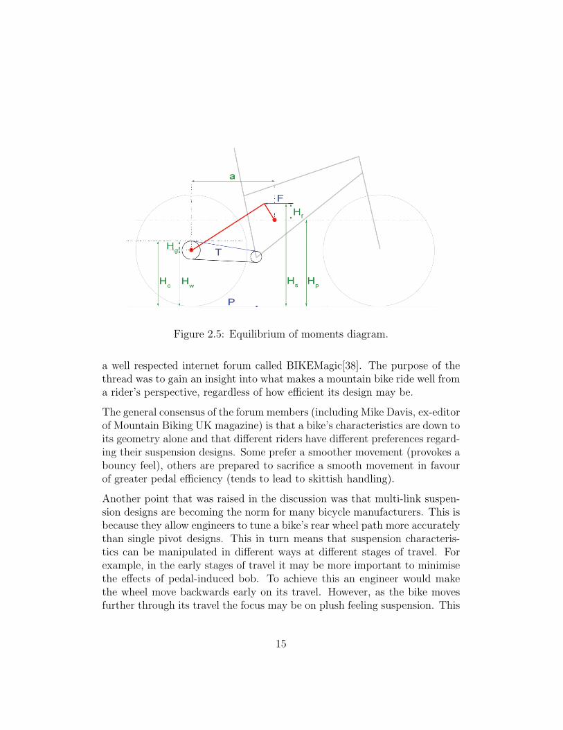
Figure 2.5: Equilibrium of moments diagram.

a well respected internet forum called BIKEMagic[38]. The purpose of thethread was to gain an insight into what makes a mountain bike ride well froma rider’s perspective, regardless of how efficient its design may be.

The general consensus of the forum members (including Mike Davis, ex-editorof Mountain Biking UK magazine) is that a bike’s characteristics are down toits geometry alone and that different riders have different preferences regard-ing their suspension designs. Some prefer a smoother movement (provokes abouncy feel), others are prepared to sacrifice a smooth movement in favourof greater pedal efficiency (tends to lead to skittish handling).

Another point that was raised in the discussion was that multi-link suspen-sion designs are becoming the norm for many bicycle manufacturers. This isbecause they allow engineers to tune a bike’s rear wheel path more accuratelythan single pivot designs. This in turn means that suspension characteris-tics can be manipulated in different ways at different stages of travel. Forexample, in the early stages of travel it may be more important to minimisethe effects of pedal-induced bob. To achieve this an engineer would makethe wheel move backwards early on its travel. However, as the bike movesfurther through its travel the focus may be on plush feeling suspension. This

15

could be achieved keeping chain growth to a minimum.

Overall it seems that the way a bike feels is down to its geometry. This hasvery little bearing on the positioning of an optimal pivot point but does havean effect on the length of the swingarm, a parameter which will be set at theuser’s discretion. Also uncovered in the discussion were peoples preferencesfor suspension feel. Some people prefer a supple suspension feel, others prefera tighter feel. These characteristics are less a suspension design issue andmore a shock absorber setup one.

2.1.5 Analysis of Current Bike Geometries

There are many different approaches to mountain bike suspension design. Togain an understanding of what makes a good design it is important to lookat bikes that are considered to be good by the riders themselves. It is alsoimportant that bikes are compared using the same parameters, somethingwhich manufacturers tend to personalise. Figure 2.8 shows the most com-mon perception of bicycle geometry, this will be the basis for all geometricalreferences throughout this project.

There appear to be two schools of thought when it comes to single pivotmountain bike design; one is to place the pivot point as close to the bottombracket as possible, see figure 2.6. The other is to position the pivot pointa small distance above and infront of the bottom bracket, as seen in figure2.7. The benefit of positioning the pivot point close to the bottom bracket isa suspension design with very little chain growth. This results in a smoothsuspension feel with very little pedal feedback. In comparison, placing thepivot point a small distance above and in front of the pivot point will causesome chaingrowth but should limit the effects of pedal induced bob.

Since these pivot point locations are tried and tested, we can use them togain an indication of how our finished application is performing. A user whoenters parameters that strictly limit the amount of chain growth should bepresented with a pivot point position that resembles that of figure 2.6. Auser who enters more relaxed parameters with respect to chain growth shouldexpect to see a pivot point location like the one shown in figure 2.7.

16

Figure 2.6: An Kona single pivot suspension design.

Figure 2.7: A SanAndreas MountainCycle single pivot suspension design.

17

Figure 2.8: Mountain Bike Geometry Diagram [1]

2.2 Evaluation of Existing Design Systems

Since mountain bike design is a fairly specialised area, there are not manycommercially available software applications that are specific to the task.Research has shown that the majority of bike manufacturers use everydayCAD and analysis packages for the design of mountain bike frames. Theseapplications are limiting for designers because they rely on the engineer’sintuition to get the design right. In this section we will look at a few appli-cations that have been developed/are used in mountain bike development atthe moment.

The first tool that deserves to be touched upon is Pro/Engineer (often re-ferred to as Pro/E or Pro). In reality Pro/E is actually a suite of pro-grams that allow engineers to create solid models at a very high level [35].It is feature-based; whereas with some CAD packages an engineer will berequired to draw lines, arcs and circles, Pro/E allows users to specify ex-trusions, sweeps, cuts and holes. The benefit of this is that the engineer isgiven the freedom to think about the problem in hand rather than how theywill represent the model in a 3D environment. Although all these features

18

promote a free thinking approach from engineers, Pro/E still requires theuser to have a strong grasp of modeling techniques and bike design. It is forthis reason that enthusiasts/developers have created other, more specialised,tools to simplify the creation of bicycle frames.

An example of a tool that has been created by an enthusiast is a productof The Bicycle Forest. The Bicycle Forest is an innovative company thatspecialise in bike rentals. In addition to rentals they offer a tool they callBikeCAD[14] which allows users to design their own frames in a format recog-nisable to engineers.

BikeCAD is a parametric CAD tool specific to bicycles. It differs from normalCAD applications in that users are not able to edit the number of parametersin the design. Users select from a number of different classical frame tem-plates (Road Bike, Rigid Mountain Bike, Single Pivot Full-Suspension Bike,Tandem, Recumbent) and modify the frames measurements to suit theirneeds. The most useful feature (and where it benefits over Pro/E) is in itsability to assess a design’s suspension characteristics. In Pro/E an engineerwould need to export their CAD file into a separate analysis program to getan idea of the design’s suspension properties. With BikeCAD the analysisfeature is built in and available to the user throughout the design process.

BikeCAD’s suspension characteristic analysis view allows user’s to plot thedifference in rear wheel vertical travel against chainstay length10 at varyingshock compressions. It also estimates the vertical rear wheel travel and givesan indication of the amount of sag that is to be expected from the design.All information presented is in a concise, easy to understand format whichmakes the application very usable.

Another tool specific to bicycle design, which shares much of BikeCAD’sfunctionality, is Linkage[33]. Linkage gives users the opportunity to designbikes with very complicated suspension designs and view their characteristicsvia a number of graphs and diagrams. Also offered is the option of importingyour own bike design by way of file or by importing a photo and tracing itsoutline into the program.

Linkage’s suspension characteristic analysis view is far more comprehen-sive than that of BikeCAD. Users are given the opportunity to view pedal-

10area between the bottom bracket and the rear wheel center

19

kickback11 graphs, material stress graphs (lateral and horizontal), swingarmleverage ratio12 graphs and axle path graphs. With all this information (as-suming they understand it) the user will have a good understanding of howtheir design will behave once built.

The three tools outlined are all suited to bike design in different ways. Pro/Eis a tool that may hold a preference for engineers due to its flexibility and3D modeling features. Programs such as this will always have their place inmountain bike design, but are often not best suited to creating initial designs.In the case of the mountain bike, models can only be evaluated for efficiencyonce a prototype has been completed. Then follows the iterative process ofexporting the model into an analysis package, reading results, adjusting themodel and then re-exporting the updated model to see if improvements havebeen made.

In contrast to Pro/E, BikeCAD is more suited to the enthusiast with a desireto create a one off mountain bike, but who may not possess the necessaryskills to use a CAD package.

This leaves Linkage, a tool that seems to have gained popularity amongstthe bike buying public as a means of analysing existing suspension designsprior to purchase rather than being used to create new bike designs. Even so,Linkage is an extremely competent tool that is capable of very detailed 2Dbike prototyping and deserves more of a presence in the commercial designof full suspension mountain bikes.

Where all these applications fall down is in their reactive nature. All the toolsmentioned require the user to have a good understanding of the suspensiondata’s meaning and to use this understanding accordingly. Unfortunately,with this approach it is very difficult for a designer to find the optimal bal-ance between their desired design characteristics. It is for this reason thatframe design is typically the domain of experienced engineers.

2.3 Computational Problem

In order to find the optimum pivot point for our model it is necessary to bal-ance our forces optimally. To do this, some sort of search is required. There

11side effect of chain-growth.12The leverage force that is applied to the shock.

20

are many different styles of search algorithms, some which are applicable toour problem and some which are not. Search algorithms can be judged bythe following four criteria [30]:

Completeness If a solution exists, will it be found every time?

Time Complexity How long does it take to find a solution?

Space Complexity How much memory will be used executing the search?

Optimality If a solution is found, will it be the best?

Our problem will always have an optimal solution, therefore our search algo-rithm must be complete or a very good approximation. With regards timecomplexity, it would be useful if the optimal solution is found quickly butnot essential (as long as it stays within time parameters specified in the re-quirements section of this document). Again, with space complexity it is notessential that the program runs using a tiny amount of memory, but the lessmemory it uses the better. The goal of this project is to find an ideal pivotpoint for a mountain bike; therefore optimality is an important criterion.

It is expected that the search implemented will converge to a single pointor line of points on the model. Therefore an uninformed/blind search13, al-though likely to find the optimal solution, will not do it in the most efficientmanner. A better solution would be a heuristic/informed search14 which willtake less time to reach the optimal point, but either will work.

2.3.1 Uninformed/Blind Searches

It is common to represent search data structures as trees; this allows theconcept of nodes and branching to be developed. Four of the six main unin-formed search strategies are outlined below (Bidirectional and Uniform costsearches have been omitted because they are not applicable to our problem).These searches may prove to be useful in the prototype stage of the softwarebuild.

13A search where the only distinction between steps is whether a goal state has beenreached of not.

14A search that gains knowledge as it searches and makes informed decisions about itsnext step.

21

Breadth First Search: The method behind breadth first search is anexhaustive one. It begins by expanding the root node d at depth15 0 andthen goes on to expand all the nodes at d+1, d+2... d+x. Therefore thisprocess has the complexity O(bd), where b is the branching factor16. Infavour of breadth first search, it is guaranteed to find a solution if one exists,however its time and space complexity are huge. For instance (assuming abranching factor of 10) at depth 10 there will be 1010 nodes created. Thisequates to 128 days of processor time (assuming a processing speed of 1000nodes/sec and nodes of size 100 bytes each) and even worse, 111 terabytesof memory. This renders breadth first search an unrealistic problem solvingstrategy for searches above depth 3 [30].

Depth First Search: Depth first searching (commonly implemented re-cursively) is good for problems with many solutions and is often faster thanthe breadth first search. It works by always expanding the deepest nodes ofa tree until it reaches a dead end; at this point it finds its way back up thetree and expands nodes at a shallower level. All values calculated from aroute down the tree are stored in a stack and reproduced when needed. Thisresults in low memory usage since only one route is stored at any one time.The storage required by this search is only O(bm), where b is the branchingfactor and m is the maximum depth of the search. However, in the worstcase, the time complexity is O(bm) which leaves it in a similar situation asthe breadth first search with regards processing load. There is also the pos-sibility that this search method will recurse to an infinite depth. As a resultof this, depth first search is classed as incomplete.

Depth Limited Search: This is an evolution of the depth first search. Itis the same in every way but for having a limit on the depth that the searchcan descend to. Having this depth-stop eradicates the problem of a searchgetting stuck in any anomalous branches. It does however create the questionof where to set the depth-stop. Too low and no gain will be seen over theoriginal depth-first search, too high and you will never reach the goal state.As may be expected, the time complexity of the search is O(bl) and the spacecomplexity is O(bl) where l is the depth limit.

15The number of levels in a trees branching structure.16The number of new nodes that each root creates.

22

Iterative Deepening Search: This search method builds on what is im-plemented in both the depth first search and the depth limited search. Theiterative deepening search takes advantage of the aforementioned searches’exponential nature by varying the depth limiter. Exactly the same methodas the depth limited search is implemented, but the search is run many timeswith an incrementing depth parameter. For example, in a problem that has asolution at depth 5, it may be reasonable (with a depth limited search) to seta depth of 10. This is a huge waste of resources, because all searching beyondthe depth 5 is needless. Even if the depth limited search were to be luckyenough to have its depth parameter set at exactly the right level, due to theexponential growth of the search, the iterative deepening search would onlybe (roughly) 11% less efficient [30]. The iterative deepening search’s timecomplexity is O(bd) and its space complexity is O(bd).

2.3.2 Heuristic/Informed Searches

Heuristic searches solve problems by learning about their environment usingtrial and error informed by rules. In doing this they are able to cut downthe number of repeated or unnecessary search steps that are made before agoal state is reached. As a result, heuristic searches have lower time andspace complexity than their uninformed counterparts. Examples of heuris-tic searches include best-first search, memory bound searches and iterativeimprovement algorithms.

Best-first Searches

Best-first searches follow similar principles to their uninformed counterparts,in particular depth-first search. However, they factor in a heuristic function17

to estimate the next node to expand. This function’s decision is based on howfar away it perceives the goal state to be. Best-first searches are often bestsuited to domains where a direct route to a goal is almost always impossible,such as route finding. It is possible to adapt the behavior of a best-firstsearch to suit a given problem. For example, the basic greedy search18 can beadapted to form an A∗ search19 simply by adding another evaluation function

17often referred to as h.18One of the simplest best-first strategies aimed at minimising the estimated cost to

reach the goal.[30]19An adaption of greedy search aimed at minimising the total path cost.[30]

23

to the decision process. This new evaluation function gains inspiration fromuniform-cost search.

Memory Bounded Searches

Memory bounded searches (as referred to previously) are a class of searchtechniques aimed at keeping space complexity to a minimum. Two wellknown searches of this type are IDA∗ (Iterative Deepening A∗) and SMA∗

(Simplified Memory-Bounded A∗), both are adaptations of the A∗ search in-tended to minimise memory usage. In the case of IDA∗, one of the mostmemory friendly blind searches has been optimised further by integrating itwith an A∗ search strategy. The result is an optimal and complete searchroutine, subject to the same conditions as the A∗ search, but that only re-quires enough memory to store one route through a tree. A good estimateof the storage requirements of IDA∗ is bd, where b is the breadth and d thedepth of the tree being searched.

IDA∗’s downfall is that it is not good at solving problems similar to that ofthe traveling salesman20. This is because its heuristic value must change forevery state that it is in. It follows that IDA∗’s complexity in the worst caseis O(N2) where N is the number of nodes to expand.

SMA∗ search attempts to overcome IDA∗’s problems by allowing itself toremember as much search history as its memory allocation permits. Whenthere is not enough memory available to store the whole search tree, nodesmust be dropped; these nodes are called forgotten nodes. SMA∗’s strategyfor dropping nodes is to drop what it considers to be the least promising.

The only prerequisite of the search is that it is given enough memory tostore the shallowest of solution paths. Without enough memory to store theshallowest solution path the search loses its complete status. With regardsoptimality, the search is only ever optimally efficient when there is enoughmemory available to store the entire search tree.

SMA∗’s true strengths lie in its ability to solve notably more complicatedproblems than A∗ without suffering a large space complexity (assuming thatthe memory allocated is limited). SMA∗’s downfall however, is when its

20A common test for search routines; a salesman must visit a number of different loca-tions and wishes to do so in the shortest route possible.

24

memory allocation is too small for the problem in hand. When this is thecase, SMA∗ must continually swap nodes in and out of memory.

Iterative Improvement Algorithms

Finally, iterative improvement algorithms; these are often the most practicalof search routines due to their ability to find a goal state without followinga strict search path. A good way to understand the iterative improvementapproach to problem solving is to think of an undulating landscape where ourobjective is to find the highest peak. The job of an iterated search algorithmis to move around this landscape in search of the goal state. There are twomain types of iterative improvement algorithms, Hill Climbing and SimulatedAnnealing, both of which are applicable to our problem.

Hill-Climbing: This algorithm is simply a loop that moves in the directionof the goal. Because of its iterative nature there is no need for it to storeany of its previous states, the result is a search technique with very lowspace complexity. Unfortunately this approach may fall into a series of trapssuch as finding a local maxima21, finding a plateaux22 or finding a ridge23.It is clear that this search method will be very limited in its applicationareas if it converges to the first peak it comes across. It is for this reasonthat random-restart hill-climbing was invented. Random-restart hill-climbingconducts many hill-climbs starting at random points on the landscape andstores the result of the evaluation of the highest peak. This method convergesto a solution very quickly given a simple landscape; however, with a morecomplicated problem, say for example an NP-complete problem, then thechances are that it will not be able to find a solution in anything less thanexponential time.

Simulated Annealing: This technique exploits the way in which metalcools and freezes into a minimal energy crystalline structure [7]. When ametal cools its atoms gradually pack together. Depending on the speed atwhich the metal cools, the density of its atoms varies. If a metal is cooled

21As opposed to a global maxima; a local maxima is a peak which is high point in anarea, but not for the whole search problem.

22A flat part of the landscape which provokes the search to conduct a random walk.23A characteristic of a landscape that has a peak, but that has sides with a much steeper

gradient than its top. The search algorithm may oscillate from side to side.

25

quickly, then its atoms are not given time to settle into a densely packedstructure, the opposite is true if the metal is cooled slowly. It is similar instyle to the basic hill-climbing algorithm, but benefits from a few importantdifferences.

The benefit of simulated annealing over some other search techniques is thatthere is less chance that the process will get stuck in a local maxima. Whenimplemented to solve the hill climbing problem this technique avoids localmaxima by varying what is called the temperature (the control parameterfor the algorithm). The major benefit of this is that, unlike other searchtechniques, it is able to use its temperature to escape local maxima. Thetemperature of the algorithm can be compared to the temperature of metalwhen cooling. When the algorithm is told to act at a high temperature,big jumps are achievable, allowing the search process to get away from localmaxima. However, when the algorithm nears its goal state, it is able to coolits temperature and focus in on a more accurate solution.

The basic structure for the simulated annealing algorithm is as follows:

1. Input and asses initial solution.

2. Estimate initial solution.

3. Generate new solutions according to temperature.

4. Assess new solutions and select best.

5. Accept new solution? Yes-continue, No-goto 7.

6. Update Stores.

7. Adjust Temperature.

8. Terminate Search? Yes-continue, No-goto 3.

9. Stop.

In order to complete a simulated annealing search it is necessary to have a rep-resentation of possible solutions, a generator of random changes in solutions,a means of evaluating the problem functions and an annealing schedule24.

24An initial temperature and a set of rules for lowering it.

26

Regarding speed, simulated annealing is largely dependent on its annealingschedule. Geman[31] derived an annealing schedule which was adequate forconvergence to a goal state, but in practice, according to Lawrence Davisand Martha Steenstrup [10], was too conservative. It was considered to beconservative because many of the problems that simulated annealing is usedto find the solutions for converge naturally to a certain point or plateaux.As a result, it is not as important to spend time in higher temperatures.

The main reason for simulated annealing’s speed issues are the same as thosethat hinder annealing in real life. To get the algorithm to converge on theoptimal point it is necessary for the process to stay at certain temperaturesfor long enough, so that a good enough sample of points may be gained (as-suming there is no natural convergence to a point as we discussed previously).If this is not the case then an optimal solution may not be found.

Given an infinite amount of time, simulated annealing will find an optimalsolution, but in the real world this is impossible. What actually happens isthat a rule is defined as to how many steps the algorithm should take. Aslong as this number of steps is sufficiently high then a good approximation tothe solution will be found. Setting the limit too low would result in a searchthat has not been given time to converge to the optimal point. The sameis true of the algorithm’s temperature; if the temperature of the algorithmis cooled in steps that are too large, or not enough time is spent at eachtemperature, it may converge to the wrong point. Because of these issues itis essential that the parameters of the annealing algorithm are set correctly.

2.3.3 Conclusion

To begin with, due to our search problem being similar to other problemswhich have been solved using iterative improvement algorithms, and theirstrong links with the engineering community, it is safe to rule out all butthe iterative improvement algorithms in our hunt for a search algorithm, al-though an understanding of the problem of search and its various algorithmsis helpful.

It is imperative that our search for the optimal point does not get stuck onfalse peaks, as this would render our application useless. Therefore, it is thecase that simulated annealing is probably the most applicable solution inour problem domain. Although others may find the same result, we cannot

27

be sure that they will not get stuck in local maximas. Whereas, given thecorrect control parameters, simulated annealing is assured to find a goodapproximation to the solution.

With respect to time complexity, it is important that our search be com-pleted in a reasonable amount of time. Although simulated annealing is notconsidered to be the fastest of searches, it is possible (once we have an under-standing of its trends in convergence) to manipulate the search parametersto see performance gains.

2.4 Technology

2.4.1 Implementation Language

The language with which we implement our program is not hugely important.In the interests of code reuse, it would be nice to use an object orientedlanguage. This would give us the opportunity to define certain aspects ofour model in separate classes, in turn allowing us to easily modify the codeat a later date to include functionality for multiple pivot suspension designs.

Another consideration is the quality of the language’s graphics library. Javahas a comprehensive graphics library which is simple to use; this is not thecase for C++. A result of a good graphics library will be the ability to createa graphical representation of our model very quickly and easily.

In regards to speed, C++ is faster than Java because of its compiled form, itslack of garbage collection and increased potential for optimisation[18]. Bothlanguages are cross platform, which means that our final application will runon all of the major operating systems (Java on a virtual machine and C++on the machine’s native hardware), although Java will run on any platformwithout re-compilation.

Overall, the choice between C++ and Java is purely down to user preference.In this instance we will side with Java because of its ability to create applets,a feature which will allow us to display our application on the internet.

28

2.4.2 Compatibility with other applications

For our application to be of use in the real world it must integrate with otherapplications. The next logical step for an engineer after creating a model inour program would be to export it into a CAD package. To stop this processbeing a matter of redrawing our application’s output into another program,it would be of great use if we allowed our model to be exported via a fileformat recognisable to CAD packages.

Since the model we will be exporting may be used in any number of CADpackages, it follows that we should find a file format that is recognisable toas many of them as possible. Research has brought to our attention two fileformats: DXF and CDF.

CDF[9] (CAD Distillation Format) is a comprehensive 3D file format in-tended for use across a number of domains including medical visualisation,CAD and visual simulations. It is a product of the web 3D consortium andas such is an open source format. The web 3D consortium prides itself on itsconformity with XML standards which therefore allow CDF files to be usedin many different situations. However, because of the CDF’s wide applica-tion domain it has become rather too complicated for our needs.

In comparison, the DXF[4] (Drawing Exchange Format) is much simpler andis recognised by all the major CAD packages. There are a number of tutorialsavailable for the creation of DXF files, which will make life much easier forus when we come to program our CAD document creation routine. Shouldwe wish to implement the export function in our program we should withoutdoubt pursue this format further.

2.5 Conclusion

During this literature review we have constructed a physics model that tellsus the moments being imparted on our simulated shock position. From thiswe have learnt much about the transfer and behavior of forces in real lifeapplications. From our model we have been able to make informed decisionsas to which search algorithms will suit the domain we are working in. Theresult of which was our decision to use simulated annealing for its ability tofind near optimal solutions without getting stuck in local maxima.

29

We have learnt that public opinion regarding mountain bike suspension de-sign very much divided. The majority of people buy bikes for their framegeometry first and worry about its efficiency second. We also picked up onthe fact that the most efficient bikes are more complicated multi-link de-signs which allow designers to tune the path of the rear axle more accurately.However, we also know that there is still a demand for single pivot bikes inthe full suspension market due to their simple, robust nature.

From our research into the many areas that our project will cover, we havegained valuable knowledge of how best to approach it. We have formulateda physics model and discussed the scale of forces which will act upon it. Wehave debated how best to search for our optimum pivot point and what tech-nologies will provide us with the tools to build our application. We are nowin a position to begin the development process.

30

Chapter 3

Requirements Analysis

Our literature review has provided us with an insight into how our projectwill progress. We are now in the position to begin thinking about what isrequired of our final application. We must be careful at this stage to gathera complete set of relevant requirements to allow us to progress with the nextstage in our development process. This will in turn aid our development ofapplicable test strategies.

We will focus our requirements gathering around functional and non-functionalrequirements, user requirements and system requirements[34]. Breaking itdown in this way will promote a more focussed approach to gathering re-quirements and will provide us with a good framework from which to developour application.

3.1 Analysis

Many of our systems requirements are generic to this application area; wecan therefore look at other applications, such as those discussed in our lit-erature review, as a source for requirements. In addition, it is critical thatwe take into account user requirements so as not to repeat any mistakesthese applications may have made. In our literature review we analysed adiscussion on the popular mountain biking internet forum, BIKEMagic [38].This discussion offers some insight into what the end user requires from aMountain Bike Rear Suspension Design Optimisation program.

31

3.2 Requirements Breakdown

Our requirements will be broken down into three categories: Search, Modeland Peripheral. In breaking our problem even more, we further increase ourchances of compiling a comprehensive requirements document. Below wewill define the criteria which our requirements must meet to fall within eachcategory.

Search: For a requirement to fall within this category it must be distinctlyrelevant to a search algorithm. Any requirement that becomes apparentas a result of said search algorithm should fall into its respective groupand not be placed in this category as a matter of course.

Model: Model requirements cover requirements that relate to the bike modelin software.

Peripheral: Requirements applicable to this category shall include standarduser and software requirements along with any other requirements thatdo not fall within the other two categories.

3.3 Format of Requirements

Because some requirements are more important than others, we shall imple-ment a ranking system to differentiate them. Breaking down the require-ments in this way will allow us to focus in on more important aspects ofthe application’s design without becoming compromised by less importantrequirements. We will use standard English language to infer rank in ourrequirements as follows:

“The system must...”

This is a requirement of the highest importance. The satisfaction of thisrequirement is of critical importance to the success of the application.

“The system should...”

Not critical, but should appear in the finished application. If a more impor-tant requirement hinders the implementation of this requirement, then themore important requirement shall take precedence.

32

“It is preferred that...”

These requirements are not vital to the success of the application, but mayimprove the application beyond its elementary form.

3.4 Requirements Gathering

Due to the contrasting stages in the development of our application, it willbe necessary to use different methods to gather our requirements. In ourliterature review we studied varying sources of information, all of which willaid our process.

To begin we will consider our model; we have already looked at what moun-tain bikers require from a single pivot suspension design [38]. From thisdiscussion we unearthed an article explaining what parameters a mountainbike designer may look to optimise in their search for an optimal pivot point[15]. We can draw many requirements from this source, all of which will addto the realism of the model, and thus the product we create.

Another source from which we can draw requirements for our model are thedesigns of existing bikes. There are many single pivot suspension designs onthe market, the majority of which claim to have the best suspension designfor their intended purpose. We must be wary however, not to get drawninto compiling our list of requirements from bicycle manufacturer marketinghype, as mentioned in our discussion on the BIKEMagic forums.

Focussing on our search, we immediately uncover a trivial requirement, thatthe optimal pivot point position be found within a specified, acceptable tol-erance. However, there are many other requirements that need to be lookedinto that will make our final application usable, one of these being the timespent processing the search. To gather requirements of this nature is trickyas the speed of our search algorithm is dependent on the landscape we aresearching, language of implementation, quality of code and the hardware ourapplication is run on. However, we must give our application every chanceof being usable. It is therefore necessary that we look into user’ acceptedresponse times and build our application around this. Jakob Nielsen’s book,Usability Engineering [26], is a good source from which to gather require-ments of this nature.

Another source which may improve our understanding of acceptable search

33

speeds are the journals and books which explain the search algorithms. Themajority of these journals will offer an indication of an algorithms complex-ity. From this we can grade our search techniques as to how fast they shouldbe finding points in relation to each other.

Finally we shall look at what we have defined as our peripheral requirements.The application we are developing is fairly standard regarding its user inter-face and interactivity. As such, we can learn from the vast array of HCI1

research that has already been carried out.

When discussing matters of HCI design we shall look to the widely acceptedbook, Human Computer Interaction by Preece et al [28]. As well as usingthis book as a reference during the design stage of our application, we willuse it as a source for requirements. Doing so will ensure our application isas accessible as possible.

The application we develop will be aimed at a relatively well defined userbase in the form of engineering professionals and enthusiastic amateurs. Itis for this reason that we need not concern ourselves with the intricate de-tails of HCI techniques which, although important, will take up much of ourdevelopment time. Our requirements will therefore only include the mostrelevant of HCI requirements.

3.5 Requirements of Significant Interest

Now that we have established our requirements gathering process, we areready to collate our requirements document (appendix A). In the followingsection we shall discuss the more interesting requirements uncovered in thatdocument, according to the rules outlined earlier on in this chapter. Otherdetails, whilst important, are of less interest for the general discussion.

3.5.1 Functional

The system must find the optimal pivot point according to thealgorithm we define. The algorithm should be capable of consis-tently finding the same point over multiple runs: So as not to baffleour user, we must make sure our search consistently finds the same pivot

1Human Computer Interaction

34

point. Should there be a situation where our search reaches a plateaux, weshould specify the side of the plateaux on which our search should conclude.Our decision as to which side of the plateaux our search will stop shall beinfluenced by engineering preferences such as swingarm stiffness or suspen-sion travel. If a user specifies that the bike be capable of long travel, thenwe should lengthen the swingarm, i.e. choose a pivot point towards the backof the plateaux (nearer the front of the bike), to accommodate this.

If we still find ourselves searching on a plateaux, then we shall choose thepivot point that gives us the shortest swingarm for the travel specified bythe user. The reason for this being, a shorter swingarm promotes stiffness[11] due to the reduced leverage that the wheel can impart on the swingarm.A spinoff of choosing a shorter swingarm is that manufacturers will needless material to produce them, resulting in a design that is both lighter andcheaper to produce.

It is preferred that the method of export for projects is via CADa file: For our application to be of any use, we need a method of exportingour model’s dimensions. We could simply allow users to see the co-ordinatesof the major points of the bike in a text area; however, as most users willbe importing said co-ordinates into some form of CAD package, it would beof more use to provide them with a facility to create CAD files containingtemplates of their designs.

In our literature review we determined that the DXF file format was themost globally recognisable file format to CAD packages. After discussionwith engineers about this file type we discovered compatibility issues withSolid Edge2 and DXF files. We eventually discovered that Solid Edge requiresDXF files to be of DXF version 12 or above in order to open them. Therefore,if we decide to implement the export of DXF files in our application, we mustbe sure to produce them in accordance with the DXF version 12 guidelines.

3.5.2 Non-Functional

The system should have a user interface which responds quicklyto user input. All geometry updates should take place in around0.1 second and searching for an optimal pivot point should take

2A commonly used 3D modelling package.

35

no longer than 10 seconds. If it appears that searching will takelonger than 1 second then a notification or progress bar should bedisplayed: In accordance with research into software usability by Nielsen[26], we must be sure to make the users interaction with our application aspredictable as possible (this does not always mean fast).

Nielsen explains that a delay of only 0.1 second is permitted if the user is tofeel that the application is reacting instantaneously. In our application, thislimit relates to the changes that users may make to the bike’s geometry. Thelimit should be of concern to us as we will be performing multiple calcula-tions to redraw the frame with every change the user makes.

Because searching for a pivot point will be carried out comparatively infre-quently, and has the potential to be relatively complicated and slow, it shallfall into one of Nielsen’s other categories. If our search takes less than asecond to complete we need not worry about implementing any new featuresto alert the user as to the progress of the search, as it is likely that theirattention will still be held by our application. However, if a search takeslonger than a second, it will be necessary for us to inform the user of the thesearch’s progress. If this is the case, we will need to implement a progressbar. In doing this we are both informing the user that our application isbusy (and has not crashed), and that they have a certain amount of time tocarry out another task.

3.5.3 User

The system must offer users an accurate view of the model. Thismodel should update in realtime when a user changes a parameter:It is important that users have an idea of how the bicycle they are designingwill look in the real world. As a result of this, we will implement a preview ofhow the finished design will look once built. Although not strictly necessary,as most engineers will have preconceived ideas as to a bike’s geometry beforethey use our application, it is a nice feature to have at our disposal, especiallywhen it comes to visualising our pivot point. The preview we implement willbehave in much a similar fashion to that of BikeCAD’s[14] but will have asomewhat simpler layout.

Due to the fact that no measurements shall be taken from our preview, weneed not worry about rounding errors in our calculations when plotting our

36

model to the screen. However, our preview will be a scaled version of thereal model, as such we need to be careful when handling numbers to avoidconverting types. If a type conversion seems unavoidable, then rather thansimply casting types we shall take care to round numbers beforehand.

3.5.4 System

System requirements for our application are fairly generic to any windowbased application. As such, we will not mention them in any detail. Never-theless, there are one or two points worth touching on.

It is preferred that the search algorithm use minimal memory.However, speed of search should take precedence over said memoryusage: We should be careful to point out here that we shall not penalise asearch technique if it is memory intensive. This is because computer mem-ory has increased in size dramatically in recent times to a point where weneed not be overly concerned about running out of it. Plainly, if a searchtechnique appears to be using large amounts of memory then it may not beright for the job, but we shall balance this against the speed and accuracyat which it finds optimal pivot points.

It is preferred that the application implement Apple OS X lookand feel patches to further improve the appearance and usabilityof the application whilst running in the Apple environment: Weshall be developing our application in the Java programming language. Thislanguage makes a valiant attempt to mimic the native look and feel of theoperating system that its programs are running on. In spite of this it stillfaces difficulties in Apple’s OS X environment in the form of menu bars.In the Windows environment, menu bars are drawn as part of the mainapplication frame, but in OS X they become part of the operating system’stask bar at the top of the screen. Currently, Java applications draw menubars in the default Windows position on all platforms but, with the inclusionof a preferences file containing the correct options, this can be rectified.

37

3.6 Conclusion

During this chapter we have studied the best sources from which to gatherrequirements for our application and dismissed those which were not appli-cable. We have learned how best to export our system’s output in a mannercompatible with existing applications through discussion with everyday usersof CAD and 3D modelling programs. We have discussed matters of HCI re-lating to our interface and determined many non-functional requirements.Our list of requirements is now complete and, as such, we are ready for thenext stage in our design process.

Some of our more useful resources were applications such as BikeCAD whoseinterfaces and functionality provided us with many useful requirements. BikeCADwas our main source for gathering requirements relating to user input. Thisapplication has been proven as a useful tool in the bicycle design domain, assuch, we can be assured that any requirements taken from it are of use to us.

The requirements we have gathered are complete and take into considerationa number of sources, all relevant to the final application. Our discussionson the BIKEMagic forums, along with examination of the DirtWorld topic“Turner/Horst vs. Turner/Kona, long and geeky” [15] provide us with avaluable insight into what is required from a design perspective. To furtherimprove the quality of the design requirements, we could have discussed theapplication with an engineer possessing expert knowledge of the problemdomain. However, such engineers are few and far between.

38

Chapter 4

Design

The purpose of this chapter is to explain the process that we shall undertakein the design of our application whilst paying close attention to our recentlycollated requirements document. In forthcoming sections we will break ourprogram down into smaller, distinct elements, called modules which shallenable us to focus on the important design goals that they each represent.We shall begin by identifying our modules and how they will interact withone another.

4.1 Modularisation

The need for us to break our system into different modules is a consequenceof the very different design problems which they represent. As outlined inour requirements analysis, we have three distinct areas to focus on: search,model and peripheral. These groups were sufficient for our requirementsgathering process but may not offer enough detail for our design. In thefollowing section we shall investigate these groups and determine how bestto modularise our design in an effort to maximise ease of coding and futuredevelopment potential.

4.1.1 Module Overview

As we discussed in the previous chapter, the search element of our applicationis required to be plugable. As such, it is necessary that we define it as adistinct module, this affords us the flexibility to interchange different search

39

algorithms without the need for extra coding.

The model element of our application is slightly more complicated. Ourmodel is the basis for our whole application but has its own distinguishableelements. In our requirements we explain that our application must haveboth a parametric1 and a graphical preview of values entered by the user.There is a clear distinction between these two elements in both function andform, and, as such, we shall define them as separate modules.

The final element that we need to look at is what we describe as ‘peripheral’.This element was originally devised to include interface requirements andany other requirements relevant to our application. Nevertheless, during ourrequirements gathering process we discovered a need for users to open, saveand export their designs in the DXF file format. This functionality sharesno similarities with anything in our interface, therefore, we will define userinterface and input/output as separate modules.

4.1.2 Module Interaction

Now that we have defined our modules we need to determine how they willinteract with each other. An obvious place to start with any system is theuser interface, it is from here that all user interaction will stem. The mostapparent form of interaction in our application will be between the userinterface and the preview screens. Every time a geometric parameter is ma-nipulated by the user, the parameter’s new value shall be sent to these twomodules. In turn, these two modules shall refresh themselves to display thenew geometry.

A similar relationship, which we shall define now, is between the user inter-face and the file input/output module. This module, when prompted by theuser, shall open or save files containing the current values of the user interfacecomponents. This interaction is much the same as those described previously.However, in this instance, our user interface module and input/output mod-ule shall share a two way relationship. Interface values may be sent to ourinput/output module for saving and may also be returned to the user inter-face when a file is being opened.

The final module for which we need to define a relationship is our search

1This section will not share any functionality with the graphical preview.

40

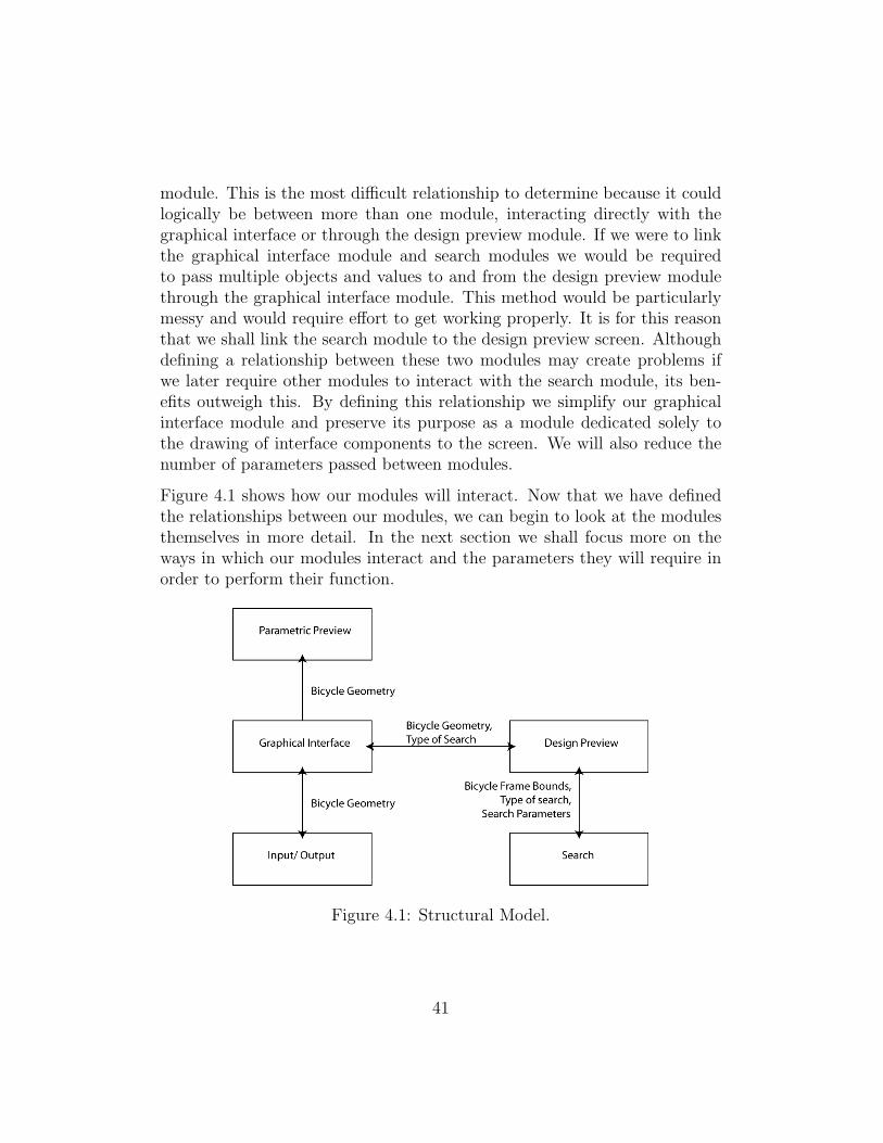
module. This is the most difficult relationship to determine because it couldlogically be between more than one module, interacting directly with thegraphical interface or through the design preview module. If we were to linkthe graphical interface module and search modules we would be requiredto pass multiple objects and values to and from the design preview modulethrough the graphical interface module. This method would be particularlymessy and would require effort to get working properly. It is for this reasonthat we shall link the search module to the design preview screen. Althoughdefining a relationship between these two modules may create problems ifwe later require other modules to interact with the search module, its ben-efits outweigh this. By defining this relationship we simplify our graphicalinterface module and preserve its purpose as a module dedicated solely tothe drawing of interface components to the screen. We will also reduce thenumber of parameters passed between modules.

Figure 4.1 shows how our modules will interact. Now that we have definedthe relationships between our modules, we can begin to look at the modulesthemselves in more detail. In the next section we shall focus more on theways in which our modules interact and the parameters they will require inorder to perform their function.

Figure 4.1: Structural Model.

41

4.1.3 Module Function

Graphical Interface Our graphical interface is the starting point for alluser interaction with our system; it is from here that users will specify thegeometry that will represent our model. In the interests of consistency weshall define a standard data structure for the storage of these design param-eters. The data structure shall comprise an array containing each interfaceparameter and shall be passed to the design preview and input/output mod-ules. Our array shall maintain its dimensions at all times and be updatedevery time a user changes a design parameter.

According to our requirements, our interface shall also allow users to definethe type of search they wish the system to perform. Consequently, we mustpass a value to our design preview (where we will be launching our searchmodule) to indicate which search method is required.

Design Preview Our design preview is the most complicated module; ittakes our predefined array and constructs our model. We must take specialcare when programming it to reuse objects at every opportunity and notcreate more objects than necessary, as this will adversely affect the speed atwhich our model is rendered [16]. As stated in our requirements, we mustmake sure that no rounding errors are made, any such errors could lead toan unrealistic model being produced and, in turn, an incorrect pivot pointlocation being found.

Another thing to consider when looking at our design preview module is thatit is directly linked to our search module. As such, it is in this module thatwe will create the necessary objects and variables to construct our search.One of the principal objects that our search module will require is the frameobject2. The frame object shall be constructed from the geometry passedfrom the graphical interface module and shall define the area in which wemay search for an optimal pivot point.

As well as drawing our bike model to the screen, our requirements specifythat we must be able to plot our search path. As such, we require our searchmodule to pass back an array of all the points that it has considered in itssearch process. It is then simply a case of looping through said array andplotting its co-ordinates to the screen.

2A digital representation of our bicycle frame.

42

Parametric Preview Our parametric preview is a fairly simple moduledue to the fact that, as stated in our requirements, it is only required toupdate three fields: effective top tube length, wheelbase length and effectivechainstay length. To calculate the values for these fields we will need theframe object that we defined earlier. From this object we can extract dimen-sions and apply the appropriate geometric calculations to give us the valueswe need in order to populate our fields. Again, all values in this module shallbe updated for every alteration the user makes to the graphical interface’sparameters.

Input/Output This is a relatively straightforward module, its main pur-pose is as a file handler, but it shall also be used to export our frame objectto a DXF file. When functioning as a file handler, having been given aninstruction to save, our module shall take the geometry array and store itsvalues in a text file with the appropriate extension. If a user then wishesto open this file, the file handler will retrieve all geometry values and returna new array mimicking the structure of our standardised geometry array tothe graphical interface module.

As mentioned previously, this module shall also be used as a method forexporting our frame object to a DXF file, from here it can be opened in themajority of CAD applications. The export process will follow the same pro-cess as the save process. However, instead of defining our own file structure,we shall adhere to that of DXF version 12. When we come to implement ourDXF file generator, we shall refer to the online manual at autodesk.com[3].

Search As we mentioned earlier in this section, our search module shall beplugable. This affords us the flexibility to try many different search tech-niques to find our optimal pivot point. Each of these search methods willrequire us to provide a boundary to the search in order for our pivot point tofall within the bounds of the frame. This boundary shall take the form of ourframe object. All search modules implemented must take this object as anargument and shall return a two dimensional point representing our optimalpivot point. Again, as stated in our requirements, we must keep track ofall searches made; we shall do this using Java’s ArrayList object. By usingthis we negate the need to continually define new array objects as our arraygrows in size, allowing our application to run faster.

43

4.2 User Interface Design

Now that we have defined our application’s behaviour we can begin to lookat the design process at a higher level. The design of an applications userinterface is critical to its success, a good user interface should appear trans-parent to the user [28]. Much research has gone into interface design in thelast ten to fifteen years, the result of which are countless rules and guidelinesby which software developers are advised to adhere. In the design of ourapplication’s user interface we shall try to act in accordance with as many ofthese as possible in the hope of creating an interface which is as transparentas possible.

We shall begin by listing the user interface components that our applicationmust display.

• Open, Save, Save As, Export as DXF.

• All search types.

• Trace whole search, Trace optimal search.

• Search.

• Chain growth and permitted travel.

• Bicycle geometry fields.

• Design preview.

• Parametric preview.

One of Shneiderman’s “Eight Golden Rules of Dialog Design” [32] states thatdevelopers should strive for consistency in their interfaces. Consequently weshall keep our generic functions, Open, Save, Save As as and Export as DXF,positioned where users would expect to find them in any other application.The majority of applications keep such functions in a “File” menu at the topof the screen, as a result we shall do the same. A further consideration toarise from placing menus at the top of the application is the use of shortcuts,it is common for applications to allow advanced users to use keyboard short-cuts to perform the common tasks that often appear in these menus. As ithappens, this is another of Schneiderman’s eight rules and, as such, we shall

44

implement keyboard shortcuts for the most common operations: New, Save,Open and Export to DXF.

For the same reasons as stated above, we shall define a search menu allowingusers to chose between every search that our application is capable of. Dueto the discrete nature of our searches we do not wish to allow users to selectmore than one at a time. The standard Java interface component for sucha circumstance is the radio button which, although frowned upon by HCIprofessionals because of its size, is the only component applicable to our sit-uation. We therefore stand no other choice but to use radio buttons in ourmenu.

Also included in this menu, for continuity purposes, will be the options toswitch on and off the search trace. We shall use checkboxes as our user in-terface component here as their intended method of interaction matches thebehaviour of our menu items perfectly.

Another common feature of modern software applications is an accessibilitybar. This bar sits at the top of the screen, below the menu bar, and providesusers with quick access to a number of commonly used operations. We shalltake advantage of this feature to, once again, preserve consistency by addingNew, Open and Save buttons to our interface, and also to locate our Searchbutton who’s function is to allow users to search for an optimal pivot point.In the interests of accessibility our buttons will display appropriate tooltipsalong with both icons and text describing their function.

The next part of the interface shall contain all the design parameters. Un-fortunately we do not have enough space to locate all of these on the screenat the same time whilst still conserving readability. We must therefore findsome way of switching between them. Java’s standard method for gettingaround this problem is to use either a scroll bar or tabbed panes. In thisinstance we shall use tabbed panes as we have two clearly defined methodsof interaction. The first of these methods will be the JSpinner, a text boxthat allows users to cycle through values incrementally as well as enteringthem explicitly. We shall use this component with predefined bounds for allgeometric parameters with no relevance to the bicycle suspension, as thesevalues must be set accurately. For our permitted chain growth and suspen-sion travel fields we shall use something different. Since these fields are notrequired to be as accurate as their geometric counterparts we shall use JS-liders. JSliders give the user quick control over parameter values and clearly

45

indicate the limits of input. We shall now look at the next logical stage inour interface development, our preview modules.

Our preview modules require no human user input which removes some ofthe difficulty associated with human computer interaction. However, it isstill important that we make our previews as easy to understand as possible.Again, we are left in the position where we do not have enough screen spaceto accommodate both preview’s comfortably. As such, in the interests offamiliarity [17] we shall once more use tabbed panes to separate our designand parameter previews.

Our parameter preview is a fairly simple screen as it will only be displayingthree fields. Because of its simplicity there are not many things that can bedone to make it more understandable. We will nonetheless take care to labeleach field so that the user knows exactly what they are being shown.

The design view shall pose some slightly different problems for us. We mustensure that the different elements of the model can be differentiated fromone another, but also that we do not flood our inerface with colour and makeit difficult to understand. Our main aim here is to create contrast wherenecessary [2] and to draw the user’s attention to the important parts of ourmodel. We will begin by setting the colour of the parts of the bike that areof no direct importance to the search: the wheels and fork. We will colourthese objects in as dull a shade as possible so as not to draw attention tothem- black and grey respectively. Our frame represents the bounds of oursearch area and, as such, should stand out. It is for this reason that we willcolour it red; although normally used as a warning, this colour is vibrant andcontrasts well with the white background.

Something else we must consider is how to colour the search trace. In ourrequirements we define two different search traces, one that considers everysearch leaf and another that considers only those leaves which have been fol-lowed. We must take special care when choosing colours to represent thesetraces, to pick those with the highest contrast, as it is expected that the op-timal search path will have significantly fewer points rendered to the screenthan its counterpart, making viewing particularly difficult. We will chooselight green when plotting all search leaves and black when plotting all fol-lowed leaves, but shall withhold our final decision until we can see our chosencolours in the working interface.

46

Finally we come to the last element in the interface. In our requirementswe state that, if time spent in a search is longer than one second, we shouldinform the user as to its progress [19]. However, because we are unsure as tohow long our searches may take to complete, we shall only implement thisfeature if it becomes necessary.

4.3 Random Search

To enable us to test the user interface it is necessary that we develop a simplesearch module. We could simply create a module which returns any pointwithin our frame bounds. However, seeing as we have already defined ourobjective function (formula 2.5) in the literature review, we shall take a moreinformed approach to the search. The method we shall use will be a randomsearch that will create a set of randomly distributed possible locations for apivot point and analyse them in relation to our objective function. Whicheverpoint is closest to being optimal is the point that shall be returned. Thealgorithm implemented will look like so:

sample size = number of locations to try

points = 0

best point = null

while points < sample size;

point = get a random point inside our bicycle frame

score = determine the optimality of point using formula 2.5

if score is closer to 0 than existing best score

best point = current point

end if

increment points

end while

return best point

47

As we can see, this is a fairly straight forward algorithm which shall berelatively easy to implement. However, the quality of pivot points that itwill find are expected to be fairly poor. The reason for this is that thealgorithm is simply picking the best point from a random distribution. Wehave no control over where the distribution of points is in relation to ourbike’s optimal pivot point other than to increase the number of points thatwe analyse. Doing this will increase the chances of finding a better pivotpoint, but there is still every chance that we will return the best pivot pointfrom a poor distribution.

Nevertheless, we now have a search module with which to test our interface.Given a large enough sample of possible pivot point locations, we shouldsee the point being placed in roughly the area that we expect the morecomplicated searches to find.

4.4 Conclusion

This section has provided us with an insight into how we should go aboutimplementing our application. We broke our application down into moduleswhich assisted our interface design and should help us further when we beginimplementation. In addition we looked into common HCI design techniquesand applied them to our application wherever possible. This has resultedin the creation of the prototype interface that can be seen in Appendix B,figures B.1 and B.2. Finally, we designed a simple search module which willenable us to test our application.

The modules we have defined will be extremely useful when we come toimplementation. If, when implementation is being carried out, we notice aneed to change the interaction of modules in any way, we will be requiredto step back into design to ensure no errors are made that may affect therest of the coding process. Nonetheless, in an ideal world this is how ourapplication shall be structured and it is an important stage of our applicationsdevelopment.

Our interface follows many predefined HCI guidelines and, as such, should berelatively usable. However, in our design process it may have been beneficialfor us to test our interface prototype on a test bed of users to establish itsusability. Despite this, the interface we have developed is fairly simple and

48

should not pose any difficulties for the capable user group for which it isintended.

Overall, our application design has provided us with a solid basis from whichto work from when developing our application. We are now at the point wherewe can begin the implementation of our Mountain Bike Rear SuspensionOptimiser.

49

Chapter 5

Implementation

This section will be dedicated to looking at the more interesting parts ofthe development of our system. We shall pay special attention to our searchalgorithms, as these are the foundation of our application.

5.1 Interface

Our interface is fairly generic, and as such we shall not go into the intricatedetails of our implementation. It is worth mentioning however, that we willtry to use lightweight Swing components wherever possible in a bid to speedup the application at runtime. Swing also avoids the majority of difficultiesassociated with cross platform implementation of Java applications and theAWT1 [6].

Another point worth raising is the lack of suitable Java layout managerswhen dealing with forms. In our interface design prototype (appendix B,figures B.1 and B.2) we have laid out our design parameters in such a waythat we require a layout manger that provides us with a some form of gridlayout. The standard Java API provides us with more than one grid stylelayout manager, but each of these suffer the same inadequacy; they all resizecomponents sitting within them to the size of the grid element that they arepart of.

Our search for a solution to this problem has led us to a package by thename of RiverLayout [12]. This package allows us to lay our panels out

1Abstract Window Toolkit.

50

using HTML2 style tags, giving us the freedom to place interface componentswherever we like without the side effects of Java’s native layout managers.

An example of the simple style of coding that this package affords us can beseen in the following code extract3 (taken from our application’s “Geometry”tab):

geomPanel.setLayout(new RiverLayout());

geomPanel.add("p center", new JLabel(

"<html>



Set Frame Geometry:



</html>"));

5.2 Design Preview

From a usability standpoint our design preview is the most important partof our application. As mentioned in previous sections we must ensure thatchanges to the geometry by the user are rendered in real time and that spe-cial care should be taken not to create new objects.

The first obstacle that we encounter in our design preview implementationis how we draw to the screen. The common method for this in Java is tooverride a panel’s paint method. Once this has been done, the user is freeto draw wherever they like within said panel. However, drawing straight tothe screen from here is afflicted by hidden inefficiencies in the form of avoid-able system calls to methods such as InputStream.read() [20]. It is suggestedtherefore, that we use a Java’s BufferedImage class to solve this problem.

A consequence of using the BufferedImage class is that is has built in geomet-ric transformations that we can use when rendering our image to the screen.Our demand for this functionality comes as a result of the way Java has beendesigned. When drawing to the screen in Java we use screen co-ordinates(our origin is in the top left of the screen). When rendering our bicyclesgeometry to the screen we shall be working in a traditional co-ordinate space

2Hyper Text Markup Language3Extract used contains HTML in the JLabel, this is common to all Java components.

We are focussing on the first argument of the add method; “p center”

51

(origin in the bottom left of the screen). Ordinarily we would be requiredto write our own transform so that all points be drawn to the screen in thecorrect orientation. However, with the BufferedImage class we can simplydefine arguments to this object and it will do it for us.

Our basic method for drawing the bicycle to the screen shall take the userdefined geometry and plot the six basic points to the screen. We shall labelthe points from A to F, as shown in figure 5.1, and shall store their x and yco-ordinates in a 2x6 array. This array can then be used as either a referencefor further calculations, or as the basis of our bicycle frame object. It is worthnoting here that we shall use Java’s Polygon class to create the bike frame.The reason for using this class is that it will save us time when we cometo implement our search methods. The Polygon class includes methods forgetting the bounding rectangle of a polygon, as well as another method forascertaining whether a given point falls within a polygon. This will enableus to easily determine our search area. It should be made clear at this pointthat we will not attempt to glamourise the model in any way. Our model isdesigned to be functional, and as a result, any attempt to make the modellook more like a bicycle would detract from its usability and eat into ourdevelopment time.

5.3 Parametric Preview

Our parametric preview is the simplest of our modules and as such has verylittle functionality worth discussing. Our module takes the frame objectdiscussed in the previous section and extracts information from it regardingthe dimensions of our bike. This information is then displayed in the threetext fields which make up the module’s interface.

5.4 Input/Output

Implementation of this module is surprisingly straight forward. Java suppliesus with all the necessary tools for file handling, and as such we need onlyfollow common guidelines to implement them.

As mentioned in previous sections, it is necessary that we allow users to savethe contents of the bicycle geometry array. There are many ways that we

52

Figure 5.1: Bike Labelling Schema.

could go about this: for example, CSV4 or XML5 files. However, we shallchoose a simple text file and separate our values by line breaks. There areno real advantages to this method over the CSV file, it is simply a matter ofpersonal preference. To prevent confusion when a user is browsing throughtheir files we shall append an extension to our filenames. This extension willbe influenced by the name that we give our application upon completion.

In much the same way that we wrote our geometry array to a file before, weshall use the same techniques to export it to a DXF file. Our requirementsstate that the method of export should be via DXF file, version 12 or above,as such we must conform with this in our implementation.

When writing our DXF file we shall abide by the guidelines laid out in theAutoCAD manual[3]. Although comprehensive, they do highlight the amountof effort involved in complying with version 12 or above. Fortunately, thereare some applications, such as CADintosh [22], which still allow users toimport old DXF files and export them in the newer format. As such, we shall

4Comma Separated Value.5Extensible Markup Language.

53

take advantage of this fact. We will begin by writing a simple DXF exportfeature for our application, this will create a file in a format recognisable toCADintosh. From here, we shall open one of our exported files and use theCADintosh export feature to convert this into the DXF version 12+ formatwe desire. This allows us to copy the contents of the new version 12+ file intoour application and simply change the locations of the hard coded values sothat they contain the appropriate dimension variables.

5.5 Search

There are numerous methods by which we could find an optimal pivot pointfor our bicycle, many of which are outlined in our literature review. In theprevious chapter we specified that a search be given its own dedicated module.This affords us the flexibility to interchange different search techniques withminimal disruption to our existing code. In the following section we shalldiscuss our implementation of the various methods used to find an optimalpoint. We will omit the random search from this section as we have alreadydiscussed its implementation in the previous chapter.

5.5.1 Simulated Annealing

In the literature review we make a strong case for the use of simulated an-nealing as a method for finding an optimal pivot point due to its ability toavoid local minima. As such, it is clear that it should become one of oursearch modules. Rather than coding our own algorithm it would appear tomake sense that we use an implementation that is already available.

The first implementation we shall look at comes in the form of the Orbitallibrary [27]. This library, on the surface, appears to contain everything weneed in order to find our optimal pivot point. However, when we attempt touse it, it becomes apparent that the documentation supplied is not sufficientand that any attempts to implement a simulated annealing search using itwould be fraught with problems.

The next stage in our search for a simulated annealing package leads us tothe Aima library [25]. Again, on the surface, this library appears to compriseall we need for our search. However, on closer inspection we notice that ithas been written to solve a specific type of simulated annealing problem, the

54

eight puzzle. The eight puzzle problem is a search for the fewest number ofoperations it takes to arrange an eight puzzle. As such, it requires that wekeep track of the algorithm’s depth via a tree data structure. It is this datastructure that makes communication between the various classes a problem.If we were to use this library then we would end up making countless smalltweaks and many unnecessary calculations in order to find a feasible solu-tion.

It is unfortunate that we cannot use these libraries, as they both captureour modularisation theme perfectly by offering us multiple search methodswithout a considerable coding overhead. However, if we are forced to makecompromises to use them, then they are not the tools for the job. Instead,we shall code our own simulated annealing algorithm. So that we don’t haveto step back into design, we shall base our simulated annealing algorithmon the Aima classes discussed earlier. As a result, we shall have 3 classes:SimulatedAnnealing.java, PivotPoint.java and PivotPointOrdering.java. Intime, we shall discuss the purpose of these classes and the role they play inour search procedure.

As demonstrated previously, the simulated annealing algorithm is fairly sim-ple. The following code extract, taken from SimulatedAnnealing.java, showsthe basic implementation procedure and how the previously defined classesrelate to it.

public double[] search(){

//start our serch here

PivotPoint pp = new PivotPoint(frame);

PivotPointOrdering o = new PivotPointOrdering(hub, BB, travel, growth);

double[][] aList = new double[n][2];

double[][] oList = new double[n][2];

points = new ArrayList();

chosen = new ArrayList();

double[] curPivot = pp.altPivot();

do{

//Get n new random points

for(int i=0; i<n; i++){

55

aList[i] = pp.altPivot(variance, curPivot);

points.add(aList[i]);

}

//Sort and select our point according to our cooling schedule

oList = o.sort(aList);

curPivot = selectPoint(oList, temp);

chosen.add(curPivot);

//Cool and reduce variance

if(!hillClimb){variance = variance*0.95;}

temp = temp*0.95;

curDepth++;

}while(!isGoalState() && (curDepth != maxDepth));

return oList[0];

}

As can be seen, the search begins by creating new PivotPoint and Pivot-PointOrdering objects, as well as initialising aList (list of unordered pivotpoints) and oList (ordered version of aList). We also declare ‘points’ and‘chosen’, the purpose of which are to record our pivot points so that we maytrace our search path to the screen.

Before we enter our iterative search process we must determine where oursearch shall begin. We will do so with a call to PivotPoint’s altPivot, a poly-morphic method which, when supplied with no arguments, returns a randompoint within our frame. We are now ready to begin our iterative search pro-cess.

The first thing we do on entry to our loop is to collate a set of possiblenext moves from the initial position to store in aList. This is achieved viamultiple6 calls to our altPivot method. In this case however, we provide twoarguments: the variance and the current pivot point. With this informationour altPivot method can return a random point within a certain radius, de-termined by the variance, of the original point.

6Number of actual calls is decided by the parent.

56

The next stage is to decide which of the points in aList will be the point fromwhich we continue the search. We begin by ordering aList with respect tooptimality, we shall call this oList. From here we can select a point from thelist to be our new pivot point. It is at this point that we realise simulatedannealing’s strength. Rather than picking the most optimal point from oList,we are able to pick less optimal points in an effort to avoid pursuing a searchroute that may lead us to a local minima. We do so via the algorithm’s‘temperature’.

When our algorithms temperature is high7, there is a greater chance thatwe will choose a pivot point location of lower optimality. However, as weprogress our search we cool its temperature; this increases our chances ofpicking a point of greater optimality and as such, allows us to target theoptimal point. There are various ways of cooling the temperature of an algo-rithm [23]; our search uses a simple method which focusses in on points veryquickly. If we find that we are finding local minima, then we should adaptour cooling schedule so that it spends more time at higher temperatures.

This process is repeated until either we reach our optimal point or we arriveat our maximum search depth. For each loop of the algorithm we lower thevariance, making big changes in pivot point location less likely, and also thetemperature. As stated previously, the result of this is to focus the searchon our goal state. In the case of this search we shall not specify a level ofoptimality at which to stop searching, instead we shall always let our searchreach its maximum depth (although we have implemented a code stub toallow us to implement this feature if necessary). The reason for this decisionis due to the speed at which our search runs; we are finding that we canrun through the algorithm to a reasonable depth in, what HCI guidelinesconsider to be, speeds which are hardly noticeable to the user [26]. As such,there is no point in halting our search prematurely, it makes more sense tolet the search run all the way through in the knowledge that any time spentin the algorithm will increase the optimality of the point found.

For the sake of readability we skipped over some of the finer details of ouralgorithm. We shall now go back and describe our implementation of themfurther. We begin by looking at the PivotPointOrdering class. This class usesa Quick Sort algorithm to order the aList array with respect to its memberslevels of optimality. The reason we are using Quick Sort over other algo-

7Values range from 1 to 100, 100 being the hottest.

57

rithms of its type is due to the speed advantages it affords us.

We shall determine the level of a point’s optimality using the same methodseen in our random search. We can see how this method works in the follow-ing code extract taken from PivotPointOrdering.java.

public double getFCost(double[] p){

double Tx = getTx();

double Ty = getTy();

double Hw = hub[1];

double Hp = p[1];

double Hc = Hw+Hg;

double a = p[0]-hub[0];

double P = (Tx*Hg)/Hw;

//(Tx*(Hp-Hc)+PHp+Ty*a)/Hf (Objective function)

double score = (Tx*(Hp-Hc)+(P*Hp)+(Ty*a))/Hf;

double penalty = getPenalty(p); //Get penalty for chain growth.

/**remove the sign of the number to avoid negative numbers

* being considered more optimal than those closer to 0.

*/

if(score<0){score=score*-1;}

score += penalty;

return score;

}

This example shows the bare-bone structure of the method used to calculatea given point’s optimality. We begin by calculating the values of all variablesneeded to compute the turning force imparted where the shock absorbermeets the swingarm. Notice how we conform with the naming conventionsdefined in previous chapters. The next step is to carry out our calculation,the result of which shall be stored in the variable ‘score’. To see how thelandscape we are searching looks at this point, please refer to figure 5.28.

As mentioned in previous chapters, we shall penalise any pivot point if theresultant design breaks a user’s permited chain growth or suspension travel

8Please note, this figure does not take into account the bounding frame.

58

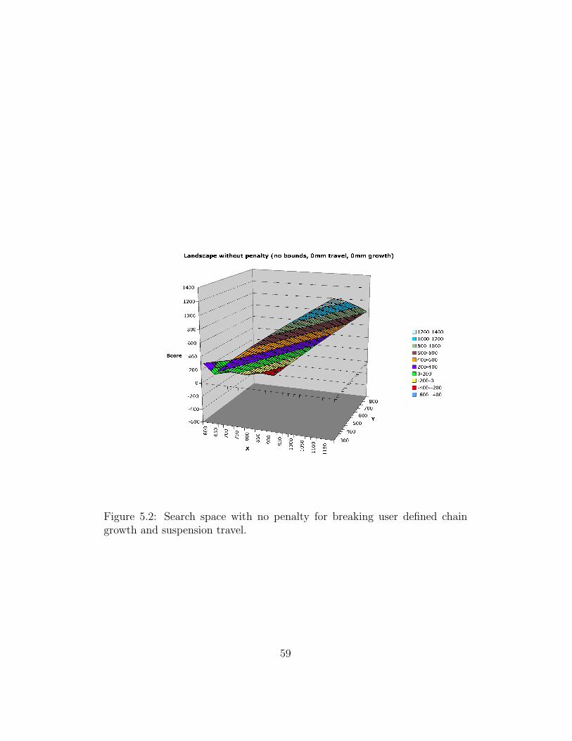
Figure 5.2: Search space with no penalty for breaking user defined chaingrowth and suspension travel.

59

tolerance. Our method for doing this, as discussed by Franco Busetti[7], isto add a large enough value to the optimality score of the offending point, inan attempt to encourage the search to disregard it. However, before we canadd said value to the optimality score, we must first make sure that ‘score’is devoid of any sign; we are searching for a point which is as close to zero aspossible and as such, are not interested in whether our design promotes chaingrowth or chain slack. Once we have done this, we may add the penalty toour signless score and return the result to the sort method. Our landscapenow resembles that of figure 5.3; note, any points falling outside the framebounds are shown as scoring 110000.

Figure 5.3: Search space with penalty, frame bounds and an accepted chaingrowth of 20mm.

A further point of interest in the search is how we select a pivot point accord-ing to the algorithm’s temperature. We studied various ways of implement-

60

ing this feature, including examining the possibilities of producing a functionwith a temperature dependent gradient, but eventually settled on a simplermethod. The method we use creates an array, equal in length to oList, anddivides it so that it contains equally distributed probability boundaries; anexample of such an array is as follows: [20,40,60,80,100]. We then multi-ply each boundary by the percentage temperature of the algorithm. Forinstance, if our temperature were at 75 we would multiply each boundary by0.75, resulting in an array like so: [15,30,45,60,100]. At this point we selecta random number between 1 and 100, whichever boundary this number fallswithin shall determine the oList element for us to return.

We should notice that at temperature 100 there is an equal chance of usreturning any of oList’s elements. However, as we reduce the temperaturewe increase the chances of the random point falling within the top bound-ary, representing the most optimal pivot point location in oList. When ourtemperature reaches 0 we have a 100 percent chance of returning the mostoptimal point.

This concludes our implementation of the classic simulated annealing algo-rithm. However, after much manipulation of annealing schedules and vari-ance values we still find the occasional anomalous pivot point. To avoid thiswe shall utilise random restarts [24], a technique more often reserved for thelikes of the basic hill climb. By doing this we reduce the speed at whichour search operates. However, this is a small price to pay if we find consis-tently optimal pivot points. Our results can be seen in figure 5.4, and clearlydemonstrate how the optimal pivot point has been targeted.

5.5.2 Consequential Search Techniques

The simulated annealing algorithm defined in the previous section sharesmany similarities with a standard hill climb. Because of this, it is possibleto modify it to create other search methods without much coding overhead.We have already discussed two techniques, random search and simulatedannealing, and in this section we shall describe two more, both of which shallbe useful when we come to test the quality of our results.

61

Figure 5.4: Sample output from our simulated annealing search.

62

Hill Climb

The first of our variations takes the form of the basic hill climb. This searchtechnique is similar to simulated annealing, but does not implement temper-ature or a reduction in variance[24]. Because it has no implementation oftemperature, it suffers from a tendency to find local minima; this may be itsdownfall when presented with our search space. Also, since it cannot reduceits variance, in the unlikely event that it were to find an optimal pivot point,it may be forced to leave it again before the search concludes. The searchtrace for this algorithm can be seen in Appendix C.2.

Variance Based Hill Climb

Our variance based search is much the same as the basic hill climb, but withthe inclusion of variance. This provides the search with the means to homein on a pivot point far better than the simple hill climb. Also, whereas thebasic hill climb may reach an optimal pivot location and have to leave dueto the search being incomplete, our variance based search will, most likely,have a small enough variance by this point that it shall still be edging evercloser to its goal state. The search trace for variance based hill climbing canbe seen in appendix C.1.

5.5.3 Conclusion

In this section we looked at the interesting aspects of our projects implemen-tation. We broke the application down into distinct modules, as outlinedin the requirements and design, allowing us to focus on the individual im-plementation problems they posed separately. As such, the final program islogical and easy to maintain.

Our implementation process would have been relatively straight forward wereit not for the fact that we struggled to find an appropriate simulated anneal-ing library. Although being able to use such libraries would have afforded usthe opportunity to test the various other search techniques on offer, we havenow gained a deeper understanding of the simulated annealing algorithm andare able to refine its parameters to best suit our needs.

In a number of previous chapters we voice concern over the speed at whichthe design preview is rendered. Initial indications of how our application

63

responds to user input are promising, we observe that the preview re-rendersin, what is essentially, real time. As such, the careful attention to detail takenduring the implementation of the design preview have not gone to waste.

The application we have produced, which can be seen in figure 5.5, appearsto be everything that we envisaged in our design. At this early stage it seemsto be finding pivot points which compare well to those of existing bicycles.This is a promising sign, but it is important that we make sure that theprogram is behaving in exactly the way it was intended. In the next chapterwe will test our application to determine whether this is the case or not.

Figure 5.5: Sample output from our simulated annealing search.

64

Chapter 6

System Testing

This chapter shall focus on ensuring our application behaves in the way weexpect it to. We shall implement various test cases to assess the accuracy ofthe implementation and, in some cases, design. Any faults discovered shallbe rectified1 and discussed. Due to the slightly experimental nature of theapplication, we shall center the majority of our resources on making sure themodel returns accurate pivot points.

Somerville [34] dictates that we may use both software inspection and soft-ware testing to verify our application. The former tests whether we haveconformed to all requirements laid out in the requirements chapter. Thelatter tests whether our application behaves in the manner expected, forinstance with black box testing.

6.1 Software Inspection

In this section, rather than discussing how our application meets every re-quirement, we shall focus on the requirements that are of most interest. Insympathy with the requirements document, and in the interests of consis-tency, we shall break this section down into its requirement types. This willpromote logical thinking which, in turn, may help to focus the inspectionprocess.

1Assuming they are not critical faults. In this instance we shall step back into thedesign phase.

65

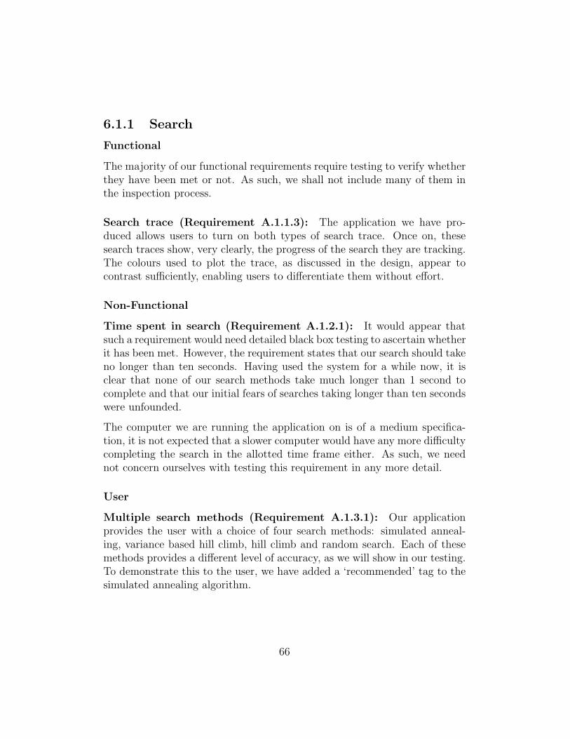
6.1.1 Search

Functional

The majority of our functional requirements require testing to verify whetherthey have been met or not. As such, we shall not include many of them inthe inspection process.

Search trace (Requirement A.1.1.3): The application we have pro-duced allows users to turn on both types of search trace. Once on, thesesearch traces show, very clearly, the progress of the search they are tracking.The colours used to plot the trace, as discussed in the design, appear tocontrast sufficiently, enabling users to differentiate them without effort.

Non-Functional

Time spent in search (Requirement A.1.2.1): It would appear thatsuch a requirement would need detailed black box testing to ascertain whetherit has been met. However, the requirement states that our search should takeno longer than ten seconds. Having used the system for a while now, it isclear that none of our search methods take much longer than 1 second tocomplete and that our initial fears of searches taking longer than ten secondswere unfounded.

The computer we are running the application on is of a medium specifica-tion, it is not expected that a slower computer would have any more difficultycompleting the search in the allotted time frame either. As such, we neednot concern ourselves with testing this requirement in any more detail.

User

Multiple search methods (Requirement A.1.3.1): Our applicationprovides the user with a choice of four search methods: simulated anneal-ing, variance based hill climb, hill climb and random search. Each of thesemethods provides a different level of accuracy, as we will show in our testing.To demonstrate this to the user, we have added a ‘recommended’ tag to thesimulated annealing algorithm.

66

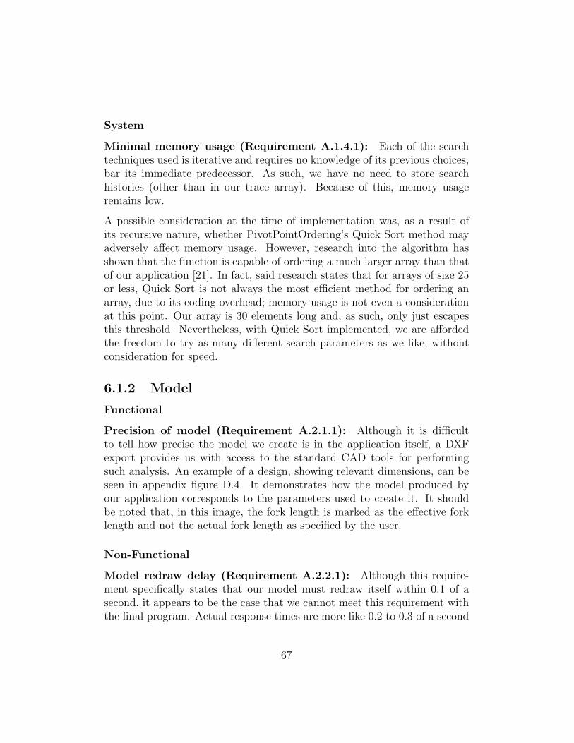
System

Minimal memory usage (Requirement A.1.4.1): Each of the searchtechniques used is iterative and requires no knowledge of its previous choices,bar its immediate predecessor. As such, we have no need to store searchhistories (other than in our trace array). Because of this, memory usageremains low.

A possible consideration at the time of implementation was, as a result ofits recursive nature, whether PivotPointOrdering’s Quick Sort method mayadversely affect memory usage. However, research into the algorithm hasshown that the function is capable of ordering a much larger array than thatof our application [21]. In fact, said research states that for arrays of size 25or less, Quick Sort is not always the most efficient method for ordering anarray, due to its coding overhead; memory usage is not even a considerationat this point. Our array is 30 elements long and, as such, only just escapesthis threshold. Nevertheless, with Quick Sort implemented, we are affordedthe freedom to try as many different search parameters as we like, withoutconsideration for speed.

6.1.2 Model

Functional

Precision of model (Requirement A.2.1.1): Although it is difficultto tell how precise the model we create is in the application itself, a DXFexport provides us with access to the standard CAD tools for performingsuch analysis. An example of a design, showing relevant dimensions, can beseen in appendix figure D.4. It demonstrates how the model produced byour application corresponds to the parameters used to create it. It shouldbe noted that, in this image, the fork length is marked as the effective forklength and not the actual fork length as specified by the user.

Non-Functional

Model redraw delay (Requirement A.2.2.1): Although this require-ment specifically states that our model must redraw itself within 0.1 of asecond, it appears to be the case that we cannot meet this requirement withthe final program. Actual response times are more like 0.2 to 0.3 of a second

67

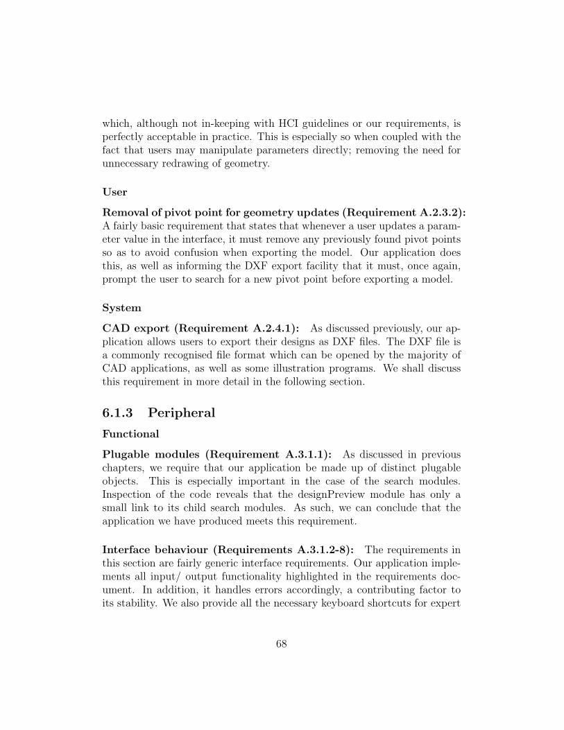
which, although not in-keeping with HCI guidelines or our requirements, isperfectly acceptable in practice. This is especially so when coupled with thefact that users may manipulate parameters directly; removing the need forunnecessary redrawing of geometry.

User

Removal of pivot point for geometry updates (Requirement A.2.3.2):A fairly basic requirement that states that whenever a user updates a param-eter value in the interface, it must remove any previously found pivot pointsso as to avoid confusion when exporting the model. Our application doesthis, as well as informing the DXF export facility that it must, once again,prompt the user to search for a new pivot point before exporting a model.

System

CAD export (Requirement A.2.4.1): As discussed previously, our ap-plication allows users to export their designs as DXF files. The DXF file isa commonly recognised file format which can be opened by the majority ofCAD applications, as well as some illustration programs. We shall discussthis requirement in more detail in the following section.

6.1.3 Peripheral

Functional

Plugable modules (Requirement A.3.1.1): As discussed in previouschapters, we require that our application be made up of distinct plugableobjects. This is especially important in the case of the search modules.Inspection of the code reveals that the designPreview module has only asmall link to its child search modules. As such, we can conclude that theapplication we have produced meets this requirement.

Interface behaviour (Requirements A.3.1.2-8): The requirements inthis section are fairly generic interface requirements. Our application imple-ments all input/ output functionality highlighted in the requirements doc-ument. In addition, it handles errors accordingly, a contributing factor toits stability. We also provide all the necessary keyboard shortcuts for expert

68

users. Finally, our parametric preview displays all necessary information, notdisplayed in the model, to the user in a clear and easy to understand manner.

Non-Functional

We have already discussed how our application responds to user input inappropriate time frames, as such, we shall not go into any more detail forthis section.

User

Chain growth and rear wheel travel (Requirements A.3.3.3-4): Ourrequirements state that users should be able to set their preferred amountof rear wheel travel and chain growth. We have implemented JSliders, dis-cussed in the design stage of this project, as the method for setting theseparameters. In practice these interface components provide satisfactory lev-els of interaction and enable users to set accurate levels of chain growth andsuspension travel.

System

Apple OS X look and feel (Requirement A.3.4.2): We have madesure that the application created implements all of OS X’s refinements. Tosee an example of this, please refer back to figure 5.5. On top of the nativelook and feel adjustments, we have also packaged the Jar executable so thatit resembles a native OS X application.

Applet conversion (Requirement A.3.4.3): Unfortunately, we havenot had time to implement this feature. Due to the way that our appli-cation uses input/ output, the conversion process is not as simple as we hadfirst hoped. Nevertheless, this is a useful feature to have in an application ofthis sort. As such, we shall consider implementing it at a later date.

6.2 Software Testing

In this section we will analyse how our application performs in various testcases in an attempt to verify its quality. We shall begin by testing ourmain search technique, simulated annealing, by using it to search simple

69

landscapes. From here, we will move on to comparing the quality of thedifferent search techniques by looking at the standard of pivot point whichthey return. We shall also consider how our applications output compares tothat of bicycles being manufactured today.

6.2.1 Simulated Annealing

The purpose of the simulated annealing algorithm is to find global maxima/minima where other techniques such as hill climbing may fail. Although ourapplication appears to be returning feasible pivot points, the landscape thatwe are searching is unknown to us. It follows therefore, that we may be find-ing local minima. It is for this reason that we must verify the quality of thealgorithm implemented on simpler landscapes that we are already familiarwith.

To perform such a test we must first adapt our simulated annealing algo-rithm to operate in a 2D environment. It is important to take special carewhen doing this, so as not to detract from the integrity of the main algo-rithm; doing so would void any test cases. Because of the versatility of thesimulated annealing function, we need simply to set the second dimensionin PivotPoints altPivot class to 0 and to change the random point generatorso that it finds points within the scale of the search. These changes, alongwith the obvious change to the objective function, will allow us to carry outtesting on various functions in a 2D environment.

Table 6.1 shows the results of a number of tests that have been carried outusing various test functions, the landscapes of which can be seen in AppendixD.1. From these results we see a reasonable level of accuracy, considering wehave not set the annealing algorithm up specifically for this task. The firstfunction we look at, sinx + 1 (figure D.1), should see our algorithm find a yvalue of zero2. Our results reflect this with a mean y value of 0.05, we alsomanage to anneal to this point relatively consistently. However, our resultsdo not reflect this as well as they should, the consequence of a single anoma-lous search.

The next function we look at is sinx ∗ cos(3∗x)+1 (figure D.2). The resultswe expect to see from this function are slightly different from that of theprevious in that we should be expecting to anneal to a value of around 0.12.

2The lowest point in a sine graph when considering the y axis.

70

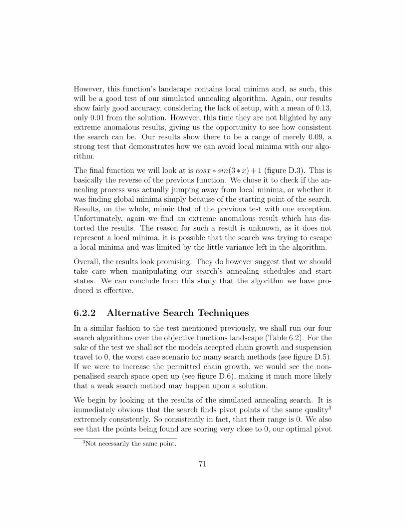
However, this function’s landscape contains local minima and, as such, thiswill be a good test of our simulated annealing algorithm. Again, our resultsshow fairly good accuracy, considering the lack of setup, with a mean of 0.13,only 0.01 from the solution. However, this time they are not blighted by anyextreme anomalous results, giving us the opportunity to see how consistentthe search can be. Our results show there to be a range of merely 0.09, astrong test that demonstrates how we can avoid local minima with our algo-rithm.

The final function we will look at is cosx ∗ sin(3 ∗x)+ 1 (figure D.3). This isbasically the reverse of the previous function. We chose it to check if the an-nealing process was actually jumping away from local minima, or whether itwas finding global minima simply because of the starting point of the search.Results, on the whole, mimic that of the previous test with one exception.Unfortunately, again we find an extreme anomalous result which has dis-torted the results. The reason for such a result is unknown, as it does notrepresent a local minima, it is possible that the search was trying to escapea local minima and was limited by the little variance left in the algorithm.

Overall, the results look promising. They do however suggest that we shouldtake care when manipulating our search’s annealing schedules and startstates. We can conclude from this study that the algorithm we have pro-duced is effective.

6.2.2 Alternative Search Techniques

In a similar fashion to the test mentioned previously, we shall run our foursearch algorithms over the objective functions landscape (Table 6.2). For thesake of the test we shall set the models accepted chain growth and suspensiontravel to 0, the worst case scenario for many search methods (see figure D.5).If we were to increase the permitted chain growth, we would see the non-penalised search space open up (see figure D.6), making it much more likelythat a weak search method may happen upon a solution.

We begin by looking at the results of the simulated annealing search. It isimmediately obvious that the search finds pivot points of the same quality3

extremely consistently. So consistently in fact, that their range is 0. We alsosee that the points being found are scoring very close to 0, our optimal pivot

3Not necessarily the same point.

71

p sinx + 1 sinx ∗ cos(3 ∗ x) + 1 cosx ∗ sin(3 ∗ x) + 11 0.106003336 0.126919629 1.05664812 0.008221147 0.126919629 0.128616953 0.231745339 0.120053215 0.1254069794 0.00431581 0.120053215 0.1211982745 9.79E-06 0.130499093 0.1292714256 2.45E-04 0.140468696 0.1794681267 0.001184775 0.126919629 0.128616958 0.003530827 0.122386606 0.1201942789 0.041075725 0.213805446 0.11991900110 0.079973962 0.120604927 0.179468126

Mean 0.047630554 0.134863009 0.228880821Range 2.32E-01 0.09375223 0.936729099

Table 6.1: Test results from trials of pivot point optimality. Please note, notall of these functions contain solutions equal to 0.

location score. This all bodes well as verification of the application’s quality.

The next test was run on the variance based hill climb. Results show similarscores to simulated annealing, if slightly less optimal (possibly a result of themethod chosen for reducing the variance). The mean score is 1.46, around0.6 higher than that of simulated annealing and the range is 0.74, again,perfectly respectable.

We now move on to the hill climb. This search is of great interest to usbecause it finds pivot point locations which have been penalised for promotingchain growth above that permitted by the user. In terms of the landscape,we can deduce that a local minima has been found, exactly the reason wechose not to use this as the application’s main search method. Were we toincrease the sample size of this test we would see that the technique findsoccasional non-penalised pivot points, and when it does, they tend to be aof a quality not dissimilar to the previous two methods.

In spite of the poor quality of results that the hill climb provides us, it isfairly consistent in its ability to find them, with a range of only 4.11. Asdiscussed in previous chapters, it is for this reason that random restart hillclimbing was invented[24]. Be that as it may, a random restart hill climbwould still stand very little chance of finding results as good as simulated

72

annealing or its variance based counterpart without tens of restarts. Theresult of so many restarts would be a comparatively lengthy search.

Finally, we look at random search. As expected, the output from this searchis hugely inconsistent, displaying a range of 61.57. It does however appearto find more optimal pivot points than the basic hill climb, with none outof the ten trials being penalised for excessive chain growth. Nonetheless,random search’s inconsistency prevents it from being a viable technique forthis domain.

Overall, the results of this test have been very interesting. Beforehand wehad no idea that our search space contained local minima, the tests haveshown this to be the case. We are moderately surprised that the variancebased hill climb does not fall into the same trap as the basic hill climb. Wecan only assume that it has a large enough variance, at a given time in itsconvergence, to skip over the local minima.

The tests show clearly that simulated annealing finds pivot points of thehighest quality, closely followed by the variance based hill climb. The nextbest technique is hard to place, due to the poor quality of results. Be thatas it may, if a user specifies that a pivot point shall not induce chain growthover a certain level then it is important that our search reflects this, even ifthe hill climb may be producing more consistent points.

p Simulated Annealing VB Hill Climb Hill Climb Random Search1 0.9120234 1.3077675 9976.4084754 12.21515382 0.9120234 2.0513272 9980.3069710 19.06915273 0.9120234 1.3077675 9976.1958964 26.16722334 0.9120234 1.3077675 9977.1459709 35.61590925 0.9120234 1.3077675 9976.1958964 21.48255196 0.9120234 1.3077675 9977.4516872 13.52215227 0.9120234 1.3077675 9977.4516872 66.99095728 0.9120234 2.0513272 9976.1958964 10.66874779 0.9120234 1.3077675 9976.4084754 12.607360610 0.9120234 1.3077675 9976.1958964 5.4193565

Mean 0.9120234 1.4564794 9977.1962850 22.37591651Range 0 0.7435597 4.1110750 61.5716007

Table 6.2: Test results from trials of pivot point optimality.

73

6.2.3 Objective Function

In this section we shall look at how our results compare to the bikes on saletoday, in an effort to verify our objective function. Unfortunately there areno set guidelines for the placement of bicycle pivot points. As such, we areforced to to test the function in an unconventional manner.

Although it may appear to be the best strategy for analysis, we shall not col-late a list of single pivot mountain bikes along with our applications approx-imation to their pivot points. This is due to the ambiguity surrounding thegeometry published by bicycle manufacturers. Instead, our analytical pro-cedure shall be to study various existing bicycle designs and pick out thosewhich display pivot points mimicking those of our application. We shall payspecial attention to the relationship between hub and bottom bracket heights,as these are the parameters most likely to affect pivot point height.

Figure 6.1: The Cannondale Prophet with DXF approximation overlay.

Our analysis has shown that the pivot points our application returns tendto be, on average, slightly lower than those of existing designs. This ismost likely due to the objective function not taking into account enough sag.

74

However, we observe a strong likeness in the program’s output to that of theCannondale Prophet. Figure 6.1 shows a DXF file, created using as manyof the geometric parameters that Cannondale supply on their website [8] aspossible4, superimposed onto an image of the bike itself.

Cannondale are a well established company who have been designing bikesfor over 35 years. The Prophet in particular receives various accolades com-mending its cross country prowess, an example of which can be seen atfeedthehabit[13].

We conclude that the pivot points found by our application are realistic,although it is difficult to quantify whether the locations it returns are anybetter than existing manufacturers’ designs. We can however draw parallelswith designs created using our program and those created by well respectedmountain bike manufacturers. As such, we may consider the objective func-tion to be of a satisfactory standard.

6.2.4 Conclusion

In this section we have discussed the software inspection and testing of themost interesting areas of our application. We have studied whether our finalproduct meets its requirements and verified the accuracy of the main searchalgorithm. On top of this, we have run tests to determine the quality of eachsearch type and the pivot points they find. We have also attempted to gaugethe accuracy of the objective function.

Software inspection has shown that we have met the vast majority of re-quirements, with only the occasional, low priority, requirement not beingimplemented. As such, the final application displays all the significant func-tionality expected of it, in the manner prescribed. This section has alsobrought to light some work which could be carried out in the future, an ex-ample of which being the conversion of our application to run in an Applet.

Moving on to look at system testing, we have been able to draw a significantamount of valuable information. The tests show our simulated annealing al-gorithm to be accurate for searching simple functions to a high degree. This,in turn, demonstrates there to be no issues regarding the search function’s

4Any parameters not supplied, or that don’t appear to match the image, will be approx-imated. It should be noted that, in this instance, no parameters affecting the positioningof the pivot point require estimation.

75

quality. What these tests do highlight however, and as we discussed earlier,is the importance of taking time to set the annealing process up properly.

In later tests we looked at how simulated annealing compares to alterna-tive search techniques. As expected, simulated annealing was proven to bethe most accurate and consistent, closely followed by the variance based hillclimb. More interesting however, was the basic hill climb’s inability to es-cape from a local minima, something that we had not picked up from ourlandscape plots (Appendix D5 and 6).

Finally, we looked at the objective function. It was difficult to determinehow best to test this because, as mentioned before, there are no set rules orguidelines for pivot point placement. The only way in which we could test thefunction, other than to build and review a bike based on our model, was tocompare the pivot points we discovered with those of bicycles already beingmanufactured. The search uncovered the Cannondale Prophet, considered tobe particularly good for riding uphill5, to be the bike utilising pivot pointsmost like those found by our application.

Overall, this section has shown our application to fulfil its design goals. Wecan see that each of the modules piece together to form a solid, reliable ap-plication that provides engineers with a sound basis from which to design asingle pivot full suspension bicycle.

5An area of mountain biking where pedal bob is at its most pronounced.

76

Chapter 7

Conclusion

The aim of this project was to create an application that, given a set of geom-etry, would automatically find a single pivot suspension bike’s optimal pivotpoint. Preliminary research uncovered the limiting factors that affect pivotpoint positioning for such bikes, as well as the methods currently applied byengineers in their design process.

We then moved on to review the existing work carried out in the variousdomains our application will cover. At this point we refined the knowledgegained in the introduction to get an idea of how the project would progress.An important part of this process was in determining the objective function,the basis for the whole project. Our approach to solving this problem was tostudy high level sources, such as forums and in some cases academic papers,to gather a set of requirements with which to discuss with Dr J.Darling.These discussions led to the creation of equation 2.5, our objective function.

Also in the literature review is a discussion of various search techniques. Thisdiscussion looks at a wide range of techniques, some of which are not appli-cable for solving the problem in hand, and explains the merits and difficultiesthey may face in relation to our application domain. We paid special atten-tion to simulated annealing, as it became apparent that it may be of use tous further on in the development process.

Another decision made in this chapter is to use the DXF file as our methodof export. This research turned out to be crucial in the usability of our ap-plication. Without it, users would have no way to export their drawings intoCAD programs and, as such, no way of continuing the design process.

77

In the next chapter we looked at what is required of the application. The pro-cess began with a study of the best places from which to draw requirementsand moved on look at those of most interest to us. We found this sectionespecially useful as a reference during our design phase, as it encapsulates allthe essential functionality of the application.

The design chapter is where we broke the application down into the distinctcomponents that we call modules. In doing this we afforded ourselves thefreedom to focus on the separate challenges which they each represent. Fol-lowing this, we defined how these modules interact and what dependenciesthey possess.

Having defined our modules, we moved on to explain their roles in furtherdetail, paying special attention to HCI guidelines wherever they may be rel-evant. In addition to this, we explained a simple method for testing theinterface that we call random search. Our explanation of this search utilisedpseudo-code to clearly define how the search executes.

Having designed the application in as much detail as possible, we were ableto move on to implementation. The project’s modularisation allowed us tobreak down our discussion of implementation into its component parts. Fromhere we discussed the more interesting challenges posed to us in the appli-cation’s development, one of which being the decision to implement our ownsimulated annealing module. This decision required that we look closely atour literature review and, where necessary, carry out further research to en-sure our implementation’s quality.

Having made the decision to write our own simulated annealing function, itbecame important that we tested it accordingly. As such, we created a seriesof tests on simple landscapes, designed to verify the accuracy at which pointswere found. The results showed good consistency when finding points, con-sidering we had not set the algorithm up specifically for the task in hand, withonly the occasional anomalous points skewing the data’s mean and range.

In addition to just testing the simulated annealing algorithm on its own, welooked at the optimality of points returned from each of the search techniqueson the objective functions landscape. The results backed up our research intothe algorithms, showing simulated annealing to be the best. However, thetests also uncovered a local minima in the objective function which we werepreviously unaware of.

78

Finally, we analysed various existing mountain bike designs in an attemptto verify our objective function, the results we received were highly satisfac-tory. We identified parallels between the pivot point locations found by ourapplication and those set on the Cannondale Prophet. The Prophet receivesvery good reviews regarding its climbing efficiency and as such, we can con-clude that our objective function provides a landscape on which to search,containing global minima representing pivot points of a high quality.

Overall, the program we have created provides users with a simple interfacefor finding optimal pivot points on single pivot mountain bikes. This givesengineers the perfect basis for further manipulation of our model in anotherapplication (see Figure 7.1). We have proven this to be the case by testingthe application’s individual components in a suitable manner and taking careto research the appropriate fields for our design. We have achieved all thisin the allotted time frame with the aid of a Gantt chart and careful projectmanagement.

7.1 Future Development

As we have already discussed, our application serves as a useful tool forthe preliminary stages in bicycle design. However, increasingly complicatedsuspension designs are becoming far more popular amongst riders, due toengineers’ greater understanding of how the rear wheel’s arc of movementaffects efficiency.

Earlier in the project we state that, time permitting, we should implementsupport for multi-link suspension designs. However, it became apparent thatthis would not be feasible given the time we had to implement the applica-tion. Therefore, this would be an obvious place to start when continuing thedevelopment of our program.

Also mentioned earlier in the project was our objective function’s low esti-mation of sag. It would be nice if a user were able to set their desired level ofsag somewhere on the interface, allowing them to tune the objective functioneven further than they can already.

Following on from the previous idea, it is possible that our application beconsidered limiting by some advanced users. As such, it may be of use toprovide these users with the tools they need to specify their own objective

79

Figure 7.1: A 3D bicycle design created in SolidEdge from our DXF file(shown).

80

functions. This would allow them to tailor the search space to their ownneeds1, possibly making the application more suited to a wider variety ofbicycle suspension applications.

1It is conceivable that an engineer may wish to optimise the location of a pivot pointfor something other than pedal bob and chain growth.

81

Bibliography

[1] Alex. Geometry 101: A rough guide to angles, lengths andstuff... 2005. http://solitudecycles.blogspot.com/2005/06/geometry-101-rough-guide-to-angles.html.

[2] Ambysoft. User interface design tips, techniques, and principles. 2006.http://www.ambysoft.com/essays/userInterfaceDesign.html.

[3] AutoCAD. Dxf reference. 2006.http://www.autodesk.com/techpubs/autocad/acadr14/dxf/.

[4] Autodesk.com. General dxf file structure. 2005.

[5] Ethos Bicycles. Suspension. 2005.

[6] Borland. Awt vs swing. 2006.http://bdn.borland.com/article/0,1410,26970,00.html.

[7] Franco Busetti. Simulated annealing overview. 2005. http://www.rose-hulman.edu/Class/ma/rader/MA477/F01/Papers/simanneal.pdf.

[8] cannondale.com. Cannondale geometry- prophet geometry chart. 2006.http://www.cannondale.com/bikes/05/geo-6.html.

[9] Web 3D consortium. Cad distillation format. 2005.

[10] Lawrence Davis. Genetic Algorithms and Simulated Annealing. Pitman,London, 1987.

[11] dirtworld.com. Cannondale introduces new fs design for 2000. 2000.http://www.dirtworld.com/productreviews/ReviewStory.asp?id=193.

82

[12] David Ekholm. Riverlayout. 2006.http://www.datadosen.se/riverlayout/.

[13] feedthehabit.com. 2005 cannondale prophet 1000 review. 2005.http://www.feedthehabit.com/.

[14] The Bicycle Forest. Full suspension bikecad. 2005.http://www.bikeforest.com/CAD/fsCAD.html.

[15] Steve from JH. Turner/horst vs. turner/kona, long and geeky. 2005.http://forums.mtbr.com/showthread.php?t=132386.

[16] Jonathan Hardwick. Optimizing java for speed. 1997.http://www.cs.cmu.edu/ jch/java/speed.html.

[17] IBM. Design basics. 2006. http://www-3.ibm.com/ibm/easy/eou ext.nsf/publish/6.

[18] Dejan Jelovic. Why java will always be slower than c++. 2005.

[19] Deborah J.Mayhew. Principles and Guidelines in Software User Inter-face Design. Prentice-Hall, Inc., 1991.

[20] Kevin Kluge. The experts talk: Thirteengreat ways to increase java performance. 1997.http://java.sun.com/developer/technicalArticles/Programming/Performance/.

[21] Michael Lamont. Quick sort. 2006. http://linux.wku.edu/ lam-onml/algor/sort/quick.html.

[22] lemkesoft. Cadintosh. 2006. http://www.lemkesoft.de/en/cadintosh.htm.

[23] Brian T. Luke. Simulated annealing cooling schedules. 2006.http://fconyx.ncifcrf.gov/ lukeb/simanf1.html.

[24] Sean Luke. Hill-climbing and simulated annealing. 2006.http://cs.gmu.edu/ sean/cs687/hillclimbing.txt.

[25] Ravi Mohan. Aima library. 2006. http://aima.cs.berkeley.edu/java-overview.html.

[26] Jakob Nielsen. Usability Engineering. AP Professional, 1994.

83

[27] Andr Platzer. Orbital library. 2006.http://www.functologic.com/orbital/.

[28] J. et al. Preece. Human Computer Interaction. Addison-Wesley Pub-lishing Company, Inc., 1994.

[29] R.AHebbert. The humble bicycle. Mech E, 1974.

[30] Russel and Norvig. Artificial Intelligence - A modern Approach, pages73–81. Prentice Hall International Publishers, 1995.

[31] Geman S. and Geman D. Stochastic relaxation-ieee transactions onpattern analysis and machine intelligence. 1984. PAMI-6, 721-741.

[32] B Shneiderman. Designing the User Interface, second edition. Addison-Wesley Publishing Company, Inc., 1992.

[33] Racooz Software. Linkage bike suspension simulation. 2005.http://www.bikechecker.com/index.php?home.

[34] Ian Somerville. Software Engineering - 6th Edition. Addison Wesley,2001.

[35] Boris Mayer St-Onge. Pro/engineer tutorial homepage. 1998.http://wwwrobot.gmc.ulaval.ca/interne/documentation/proeng/.

[36] Mountain Biking UK. Full suspension bikes- how to set them up. 2005.

[37] Unknown. Cycling kinematics. 2005.http://www.bsn.com/Cycling/articles/cycling kinematics.html.

[38] David Weldon. Suspension design dissertation. 2005.http://www.bikemagic.com/forum/forummessages/mps/dt/4/UTN/70200/V/6/SP/.

[39] Walter Zorn. Rear wheel suspension induced pedal kickback. 2002.http://www.kreuzotter.de/english/eschwinge.htm.

84

Appendix A

Requirements

A.1 Search

A.1.1 Functional

1. The system must find the optimal pivot point according to the al-gorithm we define. The algorithm should be capable of consistentlyfinding the same point over multiple runs.

2. The system should be accurate to within 5mm when finding a pivotpoint. This can be measured by finding a pivot point that falls out-side the bounds of the frame and seeing how close the point is to theboundary.

3. It is preferred that the search algorithms path may be traced to thescreen for users to analyse. Where applicable this trace should showboth considered paths and chosen paths.

A.1.2 Non-Functional

1. The system must find the optimal pivot point in under 10 seconds (inaccordance with accepted HCI guidelines).

A.1.3 User

1. It is preferred that the system allow the user to select from a numberof different search methods

85

A.1.4 System

1. It is preferred that the search algorithm use minimal memory. However,speed of search should take precedence over said memory usage.

A.2 Model

A.2.1 Functional

1. The system must use a model whose dimensions exactly (be they toscale or not) mimic that of a real world bicycle.

2. The system must provide bounds on parameters to prevent the creationof bicycles which may not be feasible in the real world. Said boundsshall not hinder the user in any way if they wish to create bicycles thatdo not adhere to preconceived ideas of what makes good mountainbike geometry; that is, users should be given creative freedom whendesigning a frame but should not be allowed to create a bicycle that isnot physically realisable.


1. It is preferred that the model redraw itself quickly (within HCI guide-lines of around 0.1 seconds) when a user alters a dimension.

A.2.3 User

1. The system must offer users an accurate view of the model. This modelshould update in realtime when a user changes a parameter.

2. The system must remove any pivot point that it may have found pre-viously from the model if a user updates any design parameters.

A.2.4 System

1. It is preferred that if the user is to save the model in a CAD format,that the CAD format be recognisable to as wide a range of applicationsas possible.

86

A.3 Peripheral

A.3.1 Functional

1. The system must be designed in such a way that allows for the plug-ing in of different search classes. By designing in such a way we giveourselves the freedom to alter/improve our system at a later date. Wealso allow ourselves the convenience of being able to test our searchalgorithms against those of others.

2. The system must allow users to save new projects.

3. The system must allow users to open existing projects.

4. The system must handle with all exceptions in appropriate manner.

5. The system must not crash.

6. The system should provide support for common shortcuts such as Saveand Open.

7. The system should use the users platforms default look and feel torender user interface components.

8. The system should provide the user with information that is relevantto the bikes design. For example; effective top tube length, wheelbaselength and effective chainstay length.

9. It is preferred that the method of export for projects is via CAD a file.


1. The system should have a user interface which responds quickly to userinput. All geometry updates should take place in around 0.1 secondand searching for an optimal pivot point should take no longer than10 seconds. If it appears that searching will take longer than 1 secondthen a notification or progress bar should be displayed.

87

A.3.3 User

1. The system must provide the user with an easy to use interface thatdisplays all relevant information in a clear manner.

2. The system must allow users to specify a bike’s head tube angle, seattube angle, seat tube length, top tube length, chainstay length, bottombracket height, wheel diameter, fork length, fork rake, head tube length,seat tube extension above top tube, head tube extension above top tubeand head tube extension below down tube.

3. The system must allow users set their accepted level of chain growth.

4. The system must allow users to set their desired amount of rear wheeltravel.

A.3.4 System

1. The system must run on any computer running the Java Runtime En-vironment.

2. It is preferred that the application implement Apple OS X look andfeel patches to further improve the appearance and usability of theapplication whilst running in the Apple environment.

3. It is preferred that the application also be bundled as an Applet toallow for the use of our application in a web browser.

88

Appendix B

Design

B.1 Prototypes

Figure B.1: View one of our interface.

89

Figure B.2: View two of our interface.

90

Appendix C

Implementation

C.1 Search Traces

Figure C.1: Sample output from a variance based hill climb search.

91

Figure C.2: Sample output from a basic hill climb search.

Figure C.3: Sample output from a random search.

92

Appendix D

Testing

D.1 Graphs

Figure D.1: sinx + 1 test graph.

93

Figure D.2: sinx ∗ cos(x ∗ 3) + 1 test graph.

94

Figure D.3: cosx ∗ sin(x ∗ 3) + 1 test graph.

95

D.2 Output

Figure D.4: DXF analysed in CAD package.

96

Figure D.5: A search landscape with no permitted chain growth or suspensiontravel.

97

Figure D.6: A search landscape with 50mm of permitted chain growth.

98

Appendix E

Code

E.1 Main.java

99

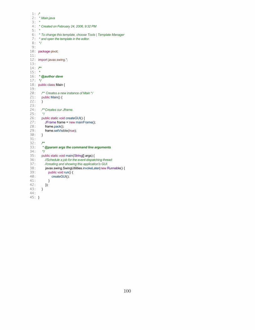
1: /*2: * Main.java3: *4: * Created on February 24, 2006, 9:32 PM5: *6: * To change this template, choose Tools | Template Manager7: * and open the template in the editor.8: */9:

10: package pivot;11:12: import javax.swing.*;13:14: /**15: *16: * @author dave17: */18: public class Main {19: 20: /** Creates a new instance of Main */21: public Main() {22: }23: 24: /**Creates our Jframe.25: */26: public static void createGUI() {27: JFrame frame = new mainFrame();28: frame.pack();29: frame.setVisible(true);30: }31: 32: /**33: * @param args the command line arguments34: */35: public static void main(String[] args) {36: //Schedule a job for the event-dispatching thread:37: //creating and showing this application's GUI.38: javax.swing.SwingUtilities.invokeLater(new Runnable() {39: public void run() {40: createGUI();41: }42: });43: }44: 45: }

100

E.2 mainFrame.java

101

1: /*2: * mainFrame.java3: *4: * Created on February 24, 2006, 9:34 PM5: *6: * To change this template, choose Tools | Template Manager7: * and open the template in the editor.8: */9:

10: package pivot;11:12: import java.awt.*;13: import java.awt.event.*;14: import java.io.File;15: import java.io.IOException;16: import java.util.Hashtable;17: import javax.swing.*;18: import javax.swing.event.*;19: import se.datadosen.component.RiverLayout;20:21:22: /**23: *24: * @author dave25: *26: * This is the JFrame from which we implement our interface.27: * Our interface includes calls to methods within the following classes:28: * - designPreview.java29: * - parametricPreview.java30: * - IOFile.java31: *32: */33: public class mainFrame extends JFrame {34: 35: /**Creates a new instance of mainFrame36: *It is from here that the majority of our high level interface37: *implementation takes place. For instance, we set the title,38: *menus and call the methods to setup the JPanels in our interface. 39: *We also determine the size of the JFrame on the screen40: *and iniialise the array containing our interface values.41: */42: public mainFrame() {43: //Make sure we have nice window decorations.44: this.setDefaultLookAndFeelDecorated(true);45: 46: initSpinMod();//initialise our geometry on left panel47: 48: //Create and set up the window.49: this.setTitle("PIVOT > Mountain Bike Rear Suspension Design Optimisation");50: this.setDefaultCloseOperation(JFrame.EXIT_ON_CLOSE);51: this.getContentPane().setLayout(new BorderLayout());52: 53: screenSize = getEnvironment();54: 55: //crate our menu bar56: JMenuBar mainMenu = new JMenuBar();57: mainMenu.add(createFileMenu());58: mainMenu.add(createSearchMenu());59: 60: createAccessibilityPanel();61: createDesignPanel();62: createControlPanel();63: createStatusPanel();64: 65: /**Add all panels to mainWindow*/66: setJMenuBar(mainMenu);

102

67: this.getContentPane().add(access, BorderLayout.NORTH);68: this.getContentPane().add(control, BorderLayout.WEST);69: this.getContentPane().add(results, BorderLayout.CENTER);70: this.getContentPane().add(status, BorderLayout.SOUTH);71: }72: 73: 74: 75: /**Get the available screen space and set the Frame position76: *to the top left of the screen.77: */78: public Dimension getEnvironment(){79: Toolkit kit = Toolkit.getDefaultToolkit();80: Dimension screenSize = kit.getScreenSize();81: GraphicsConfiguration config = this.getContentPane().getGraphicsConfiguration();82: Insets insets = kit.getScreenInsets(config);83: screenSize.width -= (insets.left + insets.right);84: screenSize.height -= (insets.top + insets.bottom);85: this.setLocation(insets.left, insets.top);86: return screenSize;87: }88: 89: 90: 91: /**Create the file menu for the menu bar92: *This menu includes:93: *-File menu94: *-Save95: *-Save As96: *-Open97: *-Export to dxf98: */99: private JMenu createFileMenu(){

100: JMenu menu = new JMenu("File");101: 102: JMenuItem newFile = new JMenuItem("New");103: newFile.setAccelerator(KeyStroke.getKeyStroke(KeyEvent.VK_N,Toolkit.getDefaultToolkit().getMenuShortcutKeyMask()));104: newFile.addActionListener(105: new ActionListener(){106: public void actionPerformed(ActionEvent e) {107: resetSpinMod();108: }109: });110: 111: 112: JMenuItem saveFile = new JMenuItem("Save");113: saveFile.setAccelerator(KeyStroke.getKeyStroke(KeyEvent.VK_S,Toolkit.getDefaultToolkit().getMenuShortcutKeyMask()));114: saveFile.addActionListener(115: new ActionListener(){116: public void actionPerformed(ActionEvent e) {117: try {118: saveFile();119: } catch (IOException ex) {120: ex.printStackTrace();121: }122: }123: });124: 125: JMenuItem saveAsFile = new JMenuItem("Save As");126: saveAsFile.addActionListener(127: new ActionListener(){128: public void actionPerformed(ActionEvent e) {129: try {130: saveAsFile();131: } catch (NullPointerException ex) {132: ex.printStackTrace();

103

133: } catch (IOException ex) {134: ex.printStackTrace();135: }136: }137: }); 138: 139: JMenuItem openFile = new JMenuItem("Open");140: openFile.setAccelerator(KeyStroke.getKeyStroke(KeyEvent.VK_O,Toolkit.getDefaultToolkit().getMenuShortcutKeyMask()));141: openFile.addActionListener(142: new ActionListener(){143: public void actionPerformed(ActionEvent e) {144: openFile();145: }146: });147: 148: JMenuItem export = new JMenuItem("Export project as \".dxf\"");149: export.setAccelerator(KeyStroke.getKeyStroke(KeyEvent.VK_E,Toolkit.getDefaultToolkit().getMenuShortcutKeyMask()));150: export.addActionListener(151: new ActionListener(){152: public void actionPerformed(ActionEvent e) { 153: try{154: if(searched){155: exportDXF(desPanel.getPoint(), desPanel.getMajorPoints(), desPanel.getWheelRadius());156: }else{157: searchForPointError();158: }159: }catch(NullPointerException n){160: searchForPointError();161: }162: }163: }); 164: 165: 166: menu.add(newFile);167: menu.add(saveFile);168: menu.add(saveAsFile);169: menu.add(openFile);170: menu.addSeparator();171: menu.add(export);172: 173: return menu;174: } 175: 176: 177: 178: /**Create our search menu.179: *This menu includes:180: *-Random Search181: *-Variance Based Hill Climb182: *-Hill Climb183: *-Simulated Annealing184: *-Trace Whole Search185: *-Trace Optimal Search186: */187: private JMenu createSearchMenu() {188: JMenu menu = new JMenu("Search");189: 190: ButtonGroup group = new ButtonGroup();191: 192: JRadioButtonMenuItem randomSearch = new JRadioButtonMenuItem("Random Search");193: randomSearch.addActionListener(194: new ActionListener(){195: public void actionPerformed(ActionEvent e) {196: desPanel.setSearchType(1);197: }198: });

104

199: 200: JRadioButtonMenuItem varianceBased = new JRadioButtonMenuItem("Variance Based Hill Climb");201: varianceBased.addActionListener(202: new ActionListener(){203: public void actionPerformed(ActionEvent e) {204: desPanel.setSearchType(2);205: }206: });207: 208: JRadioButtonMenuItem hillClimb = new JRadioButtonMenuItem("Hill Climb");209: hillClimb.addActionListener(210: new ActionListener(){211: public void actionPerformed(ActionEvent e) {212: desPanel.setSearchType(3);213: }214: });215: 216: JRadioButtonMenuItem simAnneal = new JRadioButtonMenuItem("Simulated Annealing (Recommended)");217: simAnneal.addActionListener(218: new ActionListener(){219: public void actionPerformed(ActionEvent e) {220: desPanel.setSearchType(4);221: }222: });223: 224: simAnneal.setSelected(true);225: 226: group.add(randomSearch);227: group.add(hillClimb); 228: group.add(varianceBased);229: group.add(simAnneal);230: 231: JCheckBoxMenuItem printSearch = new JCheckBoxMenuItem("Trace Whole Search");232: printSearch.addItemListener(233: new ItemListener(){234: public void itemStateChanged(ItemEvent e) {235: if (e.getStateChange() == ItemEvent.SELECTED){236: desPanel.setShowSearch(true);237: }else{238: desPanel.setShowSearch(false);239: }240: }241: });242: 243: JCheckBoxMenuItem optimSearch = new JCheckBoxMenuItem("Trace Optimal Search");244: optimSearch.addItemListener(245: new ItemListener(){246: public void itemStateChanged(ItemEvent e) {247: if (e.getStateChange() == ItemEvent.SELECTED){248: desPanel.setShowOptimalSearch(true);249: }else{250: desPanel.setShowOptimalSearch(false);251: }252: }253: });254: 255: menu.add(randomSearch);256: menu.add(hillClimb); 257: menu.add(varianceBased);258: menu.add(simAnneal);259: menu.addSeparator();260: menu.add(printSearch);261: menu.add(optimSearch);262: 263: return menu;264: }

105

265: 266: 267: 268: /**Populate our Accessibility panel. This is the panel269: *that sits in the north of our frame, below the menu.270: */271: private void createAccessibilityPanel() {272: //Create Accessibility Panel273: FlowLayout layout = new FlowLayout(FlowLayout.LEFT);274: access = new JPanel(layout);275: access.setPreferredSize(new Dimension(screenSize.width,access_height));276: 277: //Add new button278: ImageIcon newIcon = new ImageIcon("images/notepad.png");279: JButton newDoc = new JButton("New",newIcon);280: newDoc.setToolTipText("Click here to create a new design.");281: newDoc.addActionListener(282: new ActionListener() {283: public void actionPerformed(ActionEvent e) {284: resetSpinMod();285: }286: });287: 288: //Add save button289: ImageIcon saveIcon = new ImageIcon("images/floppy.png");290: JButton save = new JButton("Save",saveIcon);291: save.setToolTipText("Click here to save your current design.");292: save.addActionListener(293: new ActionListener() {294: public void actionPerformed(ActionEvent e) {295: try {296: saveFile();297: } catch (IOException ex) {298: ex.printStackTrace();299: }300: }301: });302: 303: //Add file button304: ImageIcon fileIcon = new ImageIcon("images/1f.png");305: JButton file = new JButton("Open",fileIcon);306: file.setToolTipText("Click here to open an existing design.");307: file.addActionListener(308: new ActionListener() {309: public void actionPerformed(ActionEvent e) {310: openFile();311: }312: });313: 314: ImageIcon runIcon = new ImageIcon("images/run.png");315: JButton run = new JButton("Search ",runIcon);316: run.setToolTipText("Click here to search for the optimal pivot point.");317: run.addActionListener(318: new ActionListener() {319: public void actionPerformed(ActionEvent e) {320: desPanel.search();321: paramPanel.updatePivot(desPanel.getPoint());322: searched = true;323: }324: });325: 326: access.add(newDoc);327: access.add(save);328: access.add(file);329: access.add(new Box.Filler(new Dimension(25, 25),330: new Dimension(32, 32),

106

331: new Dimension(32, 32)));332: access.add(run);333: 334: }335: 336: 337:338: /** Method for populating our suspension panel. This panel339: *comprises two JSliders.340: */341: private void popSusp() {342: JPanel labelPanel = new JPanel();343: labelPanel.setLayout(new GridLayout(1,2,0,0));344: JPanel sliderPanel = new JPanel();345: sliderPanel.setLayout(new GridLayout(1,2,0,0));346: 347: labelPanel.add(new JLabel("<html> " +348: "Set Travel</html>",349: SwingConstants.CENTER));350: labelPanel.add(new JLabel("<html> " +351: "Accepted Chain Growth </html>",352: SwingConstants.CENTER));353: 354: 355: int maxTravel = 350;356: int travelIncrement = 50;357: int maxGrowth = 50;358: int growthIncrement = 5;359: 360: travel = new JSlider(JSlider.VERTICAL, 0, 350, 0);361: travel.setMajorTickSpacing(50); // sets numbers for biggest tick marks362: travel.setMinorTickSpacing(10); // smaller tick marks363: travel.setPaintTicks(true); // display the ticks364: travel.setPaintLabels(true);365: travel.addChangeListener(366: new ChangeListener(){ //anonymous inner listener class367: public void stateChanged(ChangeEvent e) {368: int val = travel.getValue();369: desPanel.updateTravel(val); //update our desPanel with new val370: spinMod[spinMod.length-2][0] = val;//update our array of parameters371: //remind our app that it must reset its pp dues to changes372: searched = false;373: }374: });375: 376: //Add the labels to our Slider377: Hashtable travelTable = new Hashtable();378: for(int i=0; i<=maxTravel; i+=travelIncrement){379: travelTable.put(new Integer(i),new JLabel(i+"mm"));380: }381: travel.setLabelTable(travelTable);382: 383: growth = new JSlider(JSlider.VERTICAL, 0, maxGrowth, 0);384: growth.setMajorTickSpacing(growthIncrement); // sets numbers for biggest tick marks385: growth.setMinorTickSpacing(1); // smaller tick marks386: growth.setPaintTicks(true); // display the ticks387: growth.setPaintLabels(true);388: growth.addChangeListener(389: new ChangeListener(){ //anonymous inner listener class390: public void stateChanged(ChangeEvent e) {391: int val = growth.getValue();392: desPanel.updateGrowth(val);//update our desPanel with new val393: spinMod[spinMod.length-1][0] = val;//update our array of parameters394: //remind our app that it must reset its pp dues to changes395: searched = false;396: }

107

397: });398: 399: //Add the labels to our Slider400: Hashtable growthTable = new Hashtable();401: for(int i=0; i<=maxGrowth; i+=growthIncrement){402: growthTable.put(new Integer(i),new JLabel(i+"mm"));403: }404: growth.setLabelTable(growthTable);405: 406: sliderPanel.add(travel);407: sliderPanel.add(growth);408: 409: suspPanel.setLayout(new BorderLayout());410: suspPanel.add(labelPanel,BorderLayout.NORTH);411: suspPanel.add(sliderPanel,BorderLayout.CENTER);412: }413: 414: 415: 416: /**This panel loops through an array of labels and JSpinners to populate417: *our panel. So that we may update our spinners in the future we could418: *not simply create new spinners on the fly. Instead, we declare all of419: *them in a global array at the bottom of the page.420: */421: private void popGeom() {422: geomPanel.setLayout(new RiverLayout());423: geomPanel.add("p center", new JLabel(424: "<html>Set Frame Geometry:</html>"));425: 426: /**427: * A loop that runs through the "geomFields" array and populates the user interface428: * according to the its values. Spinners models are stored in the spinMod array429: */430: final double[] tmp = initGeometry;431: 432: //Loop that creates our form433: for (int i = 0; i < geomFields.length; i++) {434: JLabel l = new JLabel(geomFields[i][0]);435: geomPanel.add("p right",l);436: 437: //Create the spinner itself438: model = new SpinnerNumberModel(spinMod[i][0],439: spinMod[i][1],440: spinMod[i][2],441: spinMod[i][3]);442: //final JSpinner spinner = new JSpinner(model);443: spinner[i].setModel(model); //initialise the spnner elsewhere444: final int id = i;445: 446: //Add the listener to the spinner447: spinner[i].addChangeListener(448: new ChangeListener(){ //anonymous inner listener class449: public void stateChanged(ChangeEvent e) {450: Double val = (Double)(spinner[id].getValue());451: tmp[id] = val.doubleValue();452: desPanel.reDraw(tmp);453: paramPanel.updateFrame(desPanel.popGeometryPlot(new double[6][2]));//takes this for speed reasons454: spinMod[id][0] = val.doubleValue();455: searched = false;456: }457: });458: 459: //adjust the size of the spinner460: ftf = getTextField(spinner[i]);461: ftf.setColumns(4);462: ftf.setHorizontalAlignment(JTextField.RIGHT);

108

463: 464: //Add components to the JPanel465: l.setLabelFor(spinner[i]);466: geomPanel.add("tab hfill",spinner[i]);467: geomPanel.add(new JLabel(468: "<html>"+geomFields[i][1]+"</html>"));469: }470: }471: 472: 473: 474: /** CREATE DESIGN PANEL CONTAINER475: * From here: Turn the above into a tabbed pane, create methods/a new476: * class for the bike design which can be called multiple times to477: * to repaint them478: */479: private void createDesignPanel() {480: setGeometry();481: results = new JTabbedPane();482: 483: desPanel = new designPreview(initGeometry);484: JScrollPane design = new JScrollPane(desPanel);485: results.addTab("Design View",design);486: 487: 488: paramPanel = new parametricPreview(489: desPanel.popGeometryPlot(new double[initGeometry.length][2]));490: JScrollPane param = new JScrollPane(paramPanel);491: results.addTab("Parametric View",param);492: }493: 494: 495: 496: /** CONTROL PANEL497: * From here: Turn the above into a Tabbed Pane, create methods498: * which detail both pages. From these pages we can implement action499: * listeners500: */501: private void createControlPanel() {502: control = new JTabbedPane();503: control.setPreferredSize(new Dimension(control_width,screenSize.height-access_height-status_height));504: geomPanel = new JPanel();505: popGeom();506: JScrollPane geom = new JScrollPane(geomPanel);507: control.addTab("Geometry",geom);508: suspPanel = new JPanel();509: popSusp();510: JScrollPane susp = new JScrollPane(suspPanel);511: control.addTab("Suspension",susp);512: }513: 514: 515: 516: /**517: */518: private void createStatusPanel() {519: //Create Status panel520: status = new JPanel();521: status.setPreferredSize(new Dimension(screenSize.width,status_height));522: status.add(new JLabel("<html>© Copyright David Weldon 2006<html>"));523: }524: 525: 526: 527: /**Set our geometry initially for our designPanel528: *This only happens once, when we create our designPanel.

109

529: */530: private void setGeometry() {531: initGeometry = new double[13];532: for(int i=0; i<initGeometry.length; i++) {533: initGeometry[i] = spinMod[i][0];534: }535: }536: 537: 538: 539: /**2D array containing all information relating to geometric (poss turn to XML?)540: * parameters - start val, min val, max val, increments541: * CONTAINS FALLBACK GEOMETRY. ACTUAL GEOMETRY IS SET IN setGeometry()542: */543: public void initSpinMod(){544: spinMod = new double[][]{545: {68,45,90,0.1},546: {73,45,90,0.1},547: {410,200,1000,1},548: {560,200,1000,1},549: {435,200,1000,1},550: {340,100,1000,1},551: {650,200,1000,1},552: {500,200,1000,1},553: {10,0,200,1},554: {140,50,250,1},555: {10,0,50,1},556: {10,0,50,1},557: {10,0,50,1},558: {0,0,0,0},559: {0,0,0,0}};560: }561: 562: 563: 564: /**Used when user clicks "New" button. It resets all geometry565: *to its initial status.566: */567: public void resetSpinMod(){568: initSpinMod();569: updateSpinners(spinMod);570: updateSliders(spinMod);571: }572: 573: 574: 575: /**Used when a user opens a file. Each spinners value is updated576: *with that of the new array returned by our openFile method.577: */578: private void updateSpinners(double[][] spinMod) {579: for(int i=0; i<spinner.length; i++){580: spinner[i].setValue(new Double(spinMod[i][0]));581: }582: }583: 584: 585: 586: 587: /**Used when a user opens a file. Each slider value is updated588: *with that of the new array returned by our openFile method.589: */590: private void updateSliders(double[][] spinMod) {591: travel.setValue((int)spinMod[spinMod.length-2][0]);592: growth.setValue((int)spinMod[spinMod.length-1][0]);593: } 594:

110

595: 596: 597: /**Calls our IOFile class and updates our spinners and sliders598: *with the values contained within the users selected file. Also599: *contains file dialogue.600: */601: public final void openFile() throws NullPointerException{602: JFileChooser fc = new JFileChooser();603: pivotFileFilter filter = new pivotFileFilter();604: fc.setFileSelectionMode(JFileChooser.FILES_AND_DIRECTORIES);605: fc.setFileFilter(filter);606: fc.showOpenDialog(this.getContentPane());607: File file = fc.getSelectedFile();608: String path = "";609: 610: try{611: path = file.getAbsolutePath();612: }catch(NullPointerException e){} 613: 614: if(path != ""){615: IOFile iof = new IOFile();616: spinMod = iof.open(path, spinMod);617: updateSpinners(spinMod);618: updateSliders(spinMod);619: currentSavePath = file.getAbsolutePath();620: }621: }622: 623: 624:625: /**Our save file method. A simple call to Save in IOFile.626: *However, if currentPath is not set (no save has been made627: *previously) then we call saveAs.628: */629: public final void saveFile() throws IOException {630: if(currentSavePath != ""){631: IOFile iof = new IOFile();632: iof.save(currentSavePath,spinMod); //current values of spinners :s633: }else{634: saveAsFile();635: }636: } 637: 638: 639: 640: /**Saves our geometry (spinMod) to a file of the name specified641: *by the user. Also checks to see that the filename has not642: *already been taken.643: */644: public final void saveAsFile() throws IOException, NullPointerException{645: JFileChooser fc = new JFileChooser();646: pivotFileFilter filter = new pivotFileFilter();647: fc.setFileSelectionMode(JFileChooser.FILES_AND_DIRECTORIES);648: fc.setFileFilter(filter);649: fc.showSaveDialog(this.getContentPane());650: //Our fun regexp work to strip filename.651: String filename = fc.getSelectedFile().getAbsolutePath().replaceAll(".pivot","")+".pivot";652: File file = new File(filename);653: String path = "";654: 655: 656: if(file.exists()){657: JOptionPane.showMessageDialog(this,658: "File name already exists.",659: "Warning",660: JOptionPane.WARNING_MESSAGE);

111

661: }else{662: try{663: path = file.getAbsolutePath();664: }catch(NullPointerException e){665: System.out.println("Save Cancelled.");666: }667:668: if(path != ""){669: IOFile iof = new IOFile();670: iof.saveAs(path,spinMod); //current values of spinners :s671: currentSavePath = file.getAbsolutePath()+".pivot";672: }673: }674: }675: 676: 677: 678: /**Saves our geometry (spinMod) to a file of the name specified679: *by the user in the format of a dxf (drawing exchange format)680: *file. Also checks to see that the filename has not681: *already been taken.682: */683: public void exportDXF(double[] p, double[][] c, double wr){684: System.out.println("Exporting...");685: JFileChooser fc = new JFileChooser();686: DXFFileFilter filter = new DXFFileFilter();687: fc.setFileSelectionMode(JFileChooser.FILES_AND_DIRECTORIES);688: fc.setFileFilter(filter);689: fc.showSaveDialog(this.getContentPane()); 690: String filename = fc.getSelectedFile().getAbsolutePath().replaceAll(".dxf","")+".dxf";691: File file = new File(filename);692: String path = "";693: 694: 695: if(file.exists()){696: JOptionPane.showMessageDialog(this,697: "File name already exists.",698: "Warning",699: JOptionPane.WARNING_MESSAGE);700: }else{701: try{702: path = file.getAbsolutePath();703: }catch(NullPointerException e){704: System.out.println("Export Cancelled.");705: }706:707: if(path != ""){708: IOFile iof = new IOFile();709: iof.export(p,c,wr,path);710: }711: }712: }713: 714: 715: 716: /**The reason for this being a separate method is that we717: *cannot reference JOptionPane from inside a nested method.718: */719: public void searchForPointError(){720: JOptionPane.showMessageDialog(this,721: "Please search for a pivot point before exporting your \".dxf\" file. ",722: "Warning",723: JOptionPane.WARNING_MESSAGE);724: }725: 726:

112

727: 728: /**729: * A method taken from java.sun.com which allows the low level editing730: * of a spinners formatted textfield.731: */732: private JFormattedTextField getTextField(JSpinner spinner) {733: JComponent editor = spinner.getEditor();734: if (editor instanceof JSpinner.DefaultEditor) {735: return ((JSpinner.DefaultEditor)editor).getTextField();736: } else {737: System.err.println("Unexpected editor type: "738: + spinner.getEditor().getClass()739: + " isn't a descendant of DefaultEditor");740: return null;741: }742: }743: 744: 745: 746: int access_height = 60; // height of the access panel747: int status_height = 20; // height of the access panel748: int control_width = 270; // width of the control panel749: double[] initGeometry;750: double[][] spinMod;751: designPreview desPanel;752: parametricPreview paramPanel;753: Dimension screenSize;754: JPanel access;//For the accessibility panel755: JTabbedPane results;//For the design panel756: JTabbedPane control;//For the control panel757: JPanel status;//For the status panel758: JPanel geomPanel;759: JPanel suspPanel;760: String spinnerName;761: SpinnerModel model;762: JFormattedTextField ftf = null;763: String currentSavePath = "";764: boolean searched = false;765: 766: final JSpinner sp0 = new JSpinner();767: final JSpinner sp1 = new JSpinner();768: final JSpinner sp2 = new JSpinner();769: final JSpinner sp3 = new JSpinner();770: final JSpinner sp4 = new JSpinner();771: final JSpinner sp5 = new JSpinner();772: final JSpinner sp6 = new JSpinner();773: final JSpinner sp7 = new JSpinner();774: final JSpinner sp8 = new JSpinner();775: final JSpinner sp9 = new JSpinner();776: final JSpinner sp10 = new JSpinner();777: final JSpinner sp11 = new JSpinner();778: final JSpinner sp12 = new JSpinner();779: JSlider travel;780: JSlider growth;781: 782: JSpinner[] spinner = new JSpinner[]{sp0,sp1,sp2,sp3,sp4,sp5,sp6,sp7,sp8,sp9,sp10,sp11,sp12};783: 784: /**2D array containing all data relevant to form. (poss turn to XML?)785: * parameters - Label for spinner, unit measure786: */787: String[][] geomFields = {788: {"<html>Head angle: </html>","deg"},789: {"<html>Seat angle: </html>","deg"},790: {"<html><html>Seat tube length: </html>","mm"},791: {"<html>Top tube length: </html>","mm"},792: {"<html>Chainstay length: </html>","mm"},

113

793: {"<html>BB height: </html>","mm"},794: {"<html>Wheel diameter: </html>","mm"},795: {"<html>Fork length: </html>","mm"},796: {"<html>Fork rake: </html>","mm"},797: {"<html>Head tube length: </html>","mm"},798: {"<html>Seat tube extensionabove top tube: </html>","mm"},799: {"<html>Head tube extensionabove top tube: </html>","mm"},800: {"<html>Head tube extensionbelow downtube: </html>","mm"}};801:802: }803:

114

E.3 parametricPreview.java

115

1: /*2: * parametricPreview.java3: *4: * Created on March 6, 2006, 5:54 PM5: *6: * To change this template, choose Tools | Template Manager7: * and open the template in the editor.8: */9:

10: package pivot;11:12: import java.awt.*;13: import javax.swing.*;14: import se.datadosen.component.RiverLayout;15:16: /**17: *18: * @author dave19: */20: public class parametricPreview extends JPanel {21: 22: /**Creates a new instance of parametricPreview. Calls23: *getStats to initialise the values for the text fields.24: */25: public parametricPreview(double[][] geom) {26: getStats(geom); //prepare the value array27: addParameters();28: }29: 30: 31: 32: /**Add our parameter interface elements to the panel. Again,33: *we use RiverLayoutfor its ease of laying out forms.34: */35: private void addParameters(){36: this.setLayout(new RiverLayout());37: this.setBorder(BorderFactory.createEmptyBorder(10,30,10,10));38: 39: ettl = new JTextField(toString(value[0]),6);40: ettl.setEditable(false);41: wBase = new JTextField(toString(value[1]),6);42: wBase.setEditable(false);43: eStay = new JTextField(toString(value[2]),6);44: eStay.setEditable(false);45: 46: add("p left",new JLabel("<html>Parametric View: </html>"));47: add("p left",new JLabel("Effective Top Tube Length"));48: add("tab",ettl);49: add("",new JLabel("mm"));50: add("p left",new JLabel("Wheelbase"));51: add("tab",wBase);52: add("",new JLabel("mm"));53: add("p left",new JLabel("Effective Chainstay Length"));54: add("tab",eStay);55: add("",new JLabel("mm"));56: 57: }58: 59: 60: /**Get our textField values61: */62: public void getStats(double[][] geom){63: value[0] = getETTLength(geom);64: value[1] = getWheelbase(geom);65: value[2] = getChainstay(geom);66: }

116

67: 68: 69: 70: /**Set our textField values.71: */72: public void updateFrame(double[][] geom){73: getStats(geom);74: 75: ettl.setText(toString(getETTLength(geom)));76: wBase.setText(toString(getWheelbase(geom)));77: eStay.setText(toString(getChainstay(geom)));78: }79:80: 81: 82: /**Get the wheelbase of the bike.83: */84: private double getWheelbase(double[][] geom) {85: return Math.round(geom[5][0]-geom[0][0]);86: }87:88: 89: 90: /**Get the effective top tube length.91: */92: private double getETTLength(double[][] geom) {93: return Math.round(geom[3][0]-geom[2][0]);94: }95: 96: 97: 98: /**Get the effective chainstay length99: */

100: private double getChainstay(double[][] geom) {101: return Math.round(geom[1][0]-geom[0][0]);102: } 103: 104: 105: 106: /**This method is here incase we ever need to plot the107: *coordinates of our pivot point.108: */109: public void updatePivot(double[] point) throws NullPointerException{110: try{111: pivotPoint = point;112: revalidate();113: }catch(NullPointerException e){114: System.out.println("Null pointer in updatePivot");115: }116: }117: 118: 119: 120: /**Turns values into strings for display in textFields.121: */122: public String toString(double in){123: String val = "";124: return val += (int)in;125: }126: 127: 128:129: double[] pivotPoint = new double[]{0,0};130: double[] value = new double[3]; //Values of text fields131: 132: JTextField ettl;

117

133: JTextField wBase;134: JTextField eStay;135: }

118

E.4 designPreview.java

119

1: /*2: * designPreview.java3: *4: * Created on March 1, 2006, 9:45 PM5: *6: * To change this template, choose Tools | Template Manager7: * and open the template in the editor.8: *9: * N.B.: Please refer to drawing to understand method naming conventions.

10: * A,B,C,D,E,F all refer to points on the drawing.11: * Might want to include my thought pattern in the writeup12: */13:14: package pivot;15:16: import javax.swing.*;17: import java.awt.*;18: import java.awt.image.*;19: import java.util.ArrayList;20:21: /**22: *23: * @author dave24: */25: public class designPreview extends JPanel {26: 27: /** Creates a new instance of designPreview 28: */29: public designPreview(double[] geomIn) {30: geometry = geomIn;31: }32: 33: 34: 35: /**Reset the geometry array with new values.36: * Possibly listen for which box is being altered and only change that value37: */38: public void reDraw(double[] geomIn) {39: search = false;40: geometry = geomIn;41: repaint();42: }43: 44: 45: 46: /**Takes argument as empty 2d array for speed reasons.47: *Populates our geoemtryPlot array with coordinates of48: *our points (A,B,C,D,E,F)49: */50: public double[][] popGeometryPlot(double[][] geometryPlot) {51: geometryPlot = addA(geometryPlot);52: geometryPlot = addB(geometryPlot);53: geometryPlot = addC(geometryPlot);54: geometryPlot = addD(geometryPlot);55: geometryPlot = addE(geometryPlot);56: geometryPlot = addF(geometryPlot);57: 58: return geometryPlot;59: }60: 61: 62: 63: /**Locate point A64: */65: private double[][] addA(double[][] geometryPlot) {66: geometryPlot[0][0] = geometry[6]/2; //X

120

67: geometryPlot[0][1] = geometry[6]/2; //Y68: 69: return geometryPlot;70: }71: 72: 73: 74: /** Locate point B75: */76: private double[][] addB(double[][] geometryPlot) {77: //Workout shift in Y direction78: double bbDrop = (geometry[6]/2)-geometry[5]; //wheel radius - bb height79: 80: //Workout shift in X direction81: double temp = (geometry[4]*geometry[4])-(bbDrop*bbDrop);82: if (temp<0){temp=temp*(-1);} //avoid NaN case83: double effectiveCSL = Math.sqrt(temp); //Effective chainstay84: 85: //Add new coords86: geometryPlot[1][0] = geometryPlot[0][0]+effectiveCSL;87: geometryPlot[1][1] = geometryPlot[0][1]-bbDrop;88: 89: return geometryPlot;90: }91: 92: 93: 94: /**NOTE: The size of the frame is the seatpost length,95: * the extra length above the toptube is subtracted from the96: * seat tube length when drawing because it would affect the97: * shape of the bike.98: *99: * Locate point C

100: */101: private double[][] addC(double[][] geometryPlot) {102: double hypotenuse = geometry[2]-geometry[10]; //bottom bracket to top tube length103: double seatAngle = Math.toRadians(geometry[1]);104: 105: //Workout shift in X direction106: double setBack = Math.cos(seatAngle)*hypotenuse*(-1);107: 108: //Workout shift in Y direction109: double stHeight = Math.sin(seatAngle)*hypotenuse;110: 111: //Add new coords112: geometryPlot[2][0] = geometryPlot[1][0]+setBack;113: geometryPlot[2][1] = geometryPlot[1][1]+stHeight;114: 115: return geometryPlot;116: 117: }118: 119: 120: 121: /**Locate point D122: */123: private double[][] addD(double[][] geometryPlot) {124: //Size of head tube taking into account the extensions specified in125: //the last 3 options126: double headTube = geometry[9]+127: geometry[12]-128: geometry[11];129: 130: //Find the effective fork length131: double d2axle = geometry[7] + headTube;132: double eForkLength = Math.sqrt(

121

133: (d2axle*d2axle)+ //fork length134: (geometry[8]*geometry[8])); //fork rake (11=head tube extension above tt)135: 136: //Find the extra angle created by the fork offset (cah)137: double forkAngle = Math.atan(geometry[8]/d2axle);138: double angle = (90-geometry[0])+Math.toDegrees(forkAngle);139: 140: //Work out the height of the head141: double forkHeight = Math.cos(Math.toRadians(angle))*eForkLength;142: double headHeight = forkHeight+ (geometry[6]/2);143: 144: //What top tube rise does the headHeight equate to?145: double rise = headHeight-geometryPlot[2][1]; //use current height of C146: 147: //We can now compute the effective length of the top tube148: double temp = (geometry[3]*geometry[3])-(rise*rise);149: if (temp<0){temp=temp*(-1);} //avoid NaN case150: double eTopTubeLength = Math.sqrt(temp);151: 152: //Add new coords153: geometryPlot[3][0] = geometryPlot[2][0]+eTopTubeLength;154: geometryPlot[3][1] = geometryPlot[2][1]+rise;155: 156: return geometryPlot;157: }158: 159: 160: 161: /**Locate point C162: */163: private double[][] addE(double[][] geometryPlot) {164: double aHeadAngle = 90+geometry[0];165: double eHeadLength = geometry[9]- //Hypotenuse166: geometry[11]-167: geometry[12];168: 169: double headY = Math.cos(Math.toRadians(aHeadAngle))*170: eHeadLength;171: double headX = Math.sin(Math.toRadians(aHeadAngle))*172: eHeadLength;173: 174: //Add new coords175: geometryPlot[4][0] = geometryPlot[3][0]+headX;176: geometryPlot[4][1] = geometryPlot[3][1]+headY;177: 178: return geometryPlot;179: }180: 181: 182: 183: /**Locate point F184: */185: private double[][] addF(double[][] geometryPlot) {186: double eLength = geometry[7]+geometry[12]; //length of fork + bottom of head tube187: double temp = (geometry[7]*geometry[7])+188: (geometry[8]*geometry[8]);189: double axle2down = Math.sqrt(temp); 190: 191: //Find the extra angle created by the fork offset (cah)192: double forkAngle = Math.atan(geometry[8]/axle2down);193: double angle = (90-geometry[0])+194: Math.toDegrees(forkAngle);195: 196: double Xshift = Math.sin(Math.toRadians(angle))*197: axle2down;198:

122

199: //Add new coords200: geometryPlot[5][0] = geometryPlot[4][0]+Xshift;201: geometryPlot[5][1] = geometryPlot[0][1];202: 203: return geometryPlot;204: }205: 206: 207: 208: /**Allows parents to retrieve our array of points.209: */210: public double[][] getMajorPoints(){return geometryPlotGlobal;}211: 212: 213: 214: /**Allows parents to get our optimal pivot point.215: */216: public double[] getPoint(){return pivot;}217: 218: 219: 220: /**221: */222: public double getWheelRadius(){return geometry[6]/2;}223: 224: 225: 226: /**Scale our bikes geometry to fit it in the view. Note,227: *this method gets called for each change to geometry228: *to prevent our image from ourgrowing the screen. We229: *have also included a border in our calculations.230: */231: private int[][] scaleGeometry(double[][] geometryPlot) {232: //set scale233: double bikeWidth = geometry[6]+geometryPlot[5][0]-geometryPlot[0][0]+border;234: scale = (IMG_WIDTH/bikeWidth);235: offset = (border*scale)/2;236: 237: //scale geometry238: int[][] scaled = new int[geometryPlot.length][2];239: for(int i=0; i<scaled.length;i++) {240: for(int j=0; j<2; j++){241: scaled[i][j] = (int)Math.round(geometryPlot[i][j]*scale+offset);242: }243: }244: wheelWidth = (int)(Math.round(geometry[6])*scale);245: 246: return scaled;247: }248: 249: 250: 251: /**Draw our bikes wheels252: */253: private void drawWheels(int[][] geometryScaled) {254: //Rear wheel255: c.drawOval(geometryScaled[0][0]-(wheelWidth/2),256: geometryScaled[0][1]-(wheelWidth/2),257: wheelWidth,258: wheelWidth);259: //Front wheel260: c.drawOval(geometryScaled[5][0]-(wheelWidth/2),261: geometryScaled[5][1]-(wheelWidth/2),262: wheelWidth,263: wheelWidth);264: }

123

265: 266: 267: 268: /**Draw our frame to the screen.269: */270: private void drawFrame(int[][] geometryScaled) {271: //x (set them here because creating new objects is slow)272: int[] polygonX = new int[4];273: polygonX[0] = geometryScaled[1][0];274: polygonX[1] = geometryScaled[2][0];275: polygonX[2] = geometryScaled[3][0];276: polygonX[3] = geometryScaled[4][0];277: //y278: int[] polygonY = new int[4];279: polygonY[0] = geometryScaled[1][1];280: polygonY[1] = geometryScaled[2][1];281: polygonY[2] = geometryScaled[3][1];282: polygonY[3] = geometryScaled[4][1];283: 284: frame = new Polygon(polygonX,polygonY,4);285: c.drawPolygon(frame);286: }287: 288: 289: 290: 291: /**A non-scaled version of the bike frame for the search algorithm.292: *This is different to drawFrame() because we are not scaling the293: *frame. The intended purpose of this method is as the bounds294: *of our search.295: */296: private Polygon makeFrame(double[][] geometryPlot) {297: //x (set them here because creating new classes is slow)298: int[] polygonX = new int[4];299: polygonX[0] = (int)geometryPlot[1][0];300: polygonX[1] = (int)geometryPlot[2][0];301: polygonX[2] = (int)geometryPlot[3][0];302: polygonX[3] = (int)geometryPlot[4][0];303: //y304: int[] polygonY = new int[4];305: polygonY[0] = (int)geometryPlot[1][1];306: polygonY[1] = (int)geometryPlot[2][1];307: polygonY[2] = (int)geometryPlot[3][1];308: polygonY[3] = (int)geometryPlot[4][1];309: 310: frame = new Polygon(polygonX,polygonY,4);311: 312: return frame;313: }314: 315: 316: 317: /** Draws our swingarm. It is in here that we get our search318: *to provide us with the pivot point. Once we have our pivot319: *point we draw our swingarm. NOTE: we have many searches320: *defined, only one will be used at any time.321: */322: private void drawSwingarm(double[][] geometryPlot) {323: 324: double[] hubHeight = new double[2];325: hubHeight[0] = geometryPlot[0][0];326: hubHeight[1] = geometryPlot[0][1];327: 328: double[] BBheight = new double[2];329: BBheight[0] = geometryPlot[1][0];330: BBheight[1] = geometryPlot[1][1];

124

331: 332: pivot = new double[2];333: 334: switch(searchType){335: 336: case(1)://Random Search337: randomSearch rs = new randomSearch();338: pivot = rs.getOptimalPoint(339: makeFrame(geometryPlot),340: hubHeight,341: BBheight,342: travel,343: growth);344: if(showSearch){printPoints(rs.getPoints(),0);}345: break;346: case(2)://Variance Based Hill Climb347: SimulatedAnnealing vbhc = new SimulatedAnnealing(makeFrame(geometryPlot), 348: 1000, //depth349: 30, //points picked350: 0, //start temp 351: hubHeight, 352: BBheight,353: c,354: travel,355: growth,356: true,357: false,358: 100);359: pivot = vbhc.search();360: if(showSearch){printPoints(vbhc.getPoints(),0);}361: if(showSearch){printPoints(vbhc.getChosenPoints(),1);}362: break;363: case(3)://Hill Climb364: SimulatedAnnealing hc = new SimulatedAnnealing(makeFrame(geometryPlot), 365: 100, //depth366: 30, //points picked367: 0, //start temp 368: hubHeight, 369: BBheight,370: c,371: travel,372: growth,373: false,374: true,375: makeFrame(geometryPlot).getBounds().width);376: pivot = hc.search();377: if(showSearch){printPoints(hc.getPoints(),0);}378: if(showOptimalSearch){printPoints(hc.getChosenPoints(),1);}379: break;380: case(4)://Simulated Annealing381: int count = 0;382: 383: //Random restart simulated annealing384: do{385: sa = new SimulatedAnnealing(makeFrame(geometryPlot), 386: 100, //depth387: 30, //points picked388: 80, //start temp 389: hubHeight, 390: BBheight,391: c,392: travel,393: growth,394: true,395: false,396: makeFrame(geometryPlot).getBounds().width);

125

397:398: pivot = sa.search();399: count++;400: }while((sa.getFCost(pivot)>1000)&& (count < 10));401: 402: System.out.println(sa.getFCost(pivot)+". Searches made: "+count);403: 404: if(showSearch){printPoints(sa.getPoints(),0);}405: if(showOptimalSearch){printPoints(sa.getChosenPoints(),1);}406: break;407: 408: }409: 410: 411: 412: //create scaled version of our search area413: int[] swingarmScaled = new int[4];414: swingarmScaled[0] = (int)(geometryPlot[0][0]*scale+offset);415: swingarmScaled[1] = (int)(geometryPlot[0][1]*scale+offset);416: swingarmScaled[2] = (int)(pivot[0]*scale+offset);417: swingarmScaled[3] = (int)(pivot[1]*scale+offset);418: 419: //populate the array420: c.setColor(Color.BLUE);421: c.drawLine(swingarmScaled[0],422: swingarmScaled[1],423: swingarmScaled[2],424: swingarmScaled[3]);425: }426: 427: 428: 429: /**Turn on our show trace option430: */431: public void setShowSearch(boolean a){showSearch = a;}432: 433: 434: 435: /**Turn on our show optimal search option.436: */437: public void setShowOptimalSearch(boolean a){showOptimalSearch = a;}438: 439: 440: 441: /**Sets the global preferred search type selected442: *by the user in our user interface.443: */444: public void setSearchType(int typeIn){445: searchType = typeIn;446: }447: 448: 449: 450: /**Print our search trace. Colour can be either 0 or 1451: *depending on the search you are doing.452: */453: public void printPoints(ArrayList a, int colour){454: 455: switch(colour){456: case(0):c.setColor(Color.green);457: break;458: case(1):c.setColor(Color.BLACK);459: break;460: }461: 462: double[] p;

126

463: for(int i=0; i<a.size();i++){464: p = (double[])a.get(i);465: c.drawLine((int)(p[0]*scale+offset),466: (int)(p[1]*scale+offset),467: (int)(p[0]*scale+offset),468: (int)(p[1]*scale+offset));469: } 470: 471: }472: 473: 474: 475: /** Called to initiate search in its parent.476: */477: public void search() {478: search = true;479: repaint();480: }481: 482: 483: 484: /**Update the amount of travel permitted by the user. This485: *is set in out interface486: */487: public void updateTravel(int val) {488: travel = val;489: }490: 491: 492: 493: /**Update the amount of chain growth permitted by the user. This494: *is set in out interface495: */496: public void updateGrowth(int val) {497: growth = val;498: } 499: 500: 501: 502: /**Draw our fork to the screen.503: */504: private void drawFork(int[][] geometryScaled) {505: c.drawLine(geometryScaled[4][0],506: geometryScaled[4][1],507: geometryScaled[5][0],508: geometryScaled[5][1]);509: } 510: 511: 512: 513: /**Our paint component.514: */515: public void paintComponent(Graphics g) {516: 517: //Initialise JPanel518: this.setPreferredSize(new Dimension(this.getWidth(),this.getHeight()));519: IMG_WIDTH = this.getWidth()-10;520: IMG_HEIGHT = this.getHeight()-10;521: 522: //Initialise our canvas523: super.paintComponent(g);524: Graphics2D g2 = (Graphics2D)g;525: bi = new BufferedImage(IMG_WIDTH,526: IMG_HEIGHT,527: BufferedImage.TYPE_INT_RGB);528: c = bi.createGraphics();

127

529: c.setBackground(Color.WHITE);530: c.clearRect(0,0,IMG_WIDTH,IMG_HEIGHT);531: 532: //set up the geometry arrays533: double[][] geometryPlot = new double[6][2];534: int[][] geometryScaled = new int[geometryPlot.length][2];535: geometryPlotGlobal = geometryPlot;536: 537: //Begin Drawing (setStroke)538: popGeometryPlot(geometryPlot);539: geometryScaled = scaleGeometry(geometryPlot);540: c.setColor(Color.BLACK);541: drawWheels(geometryScaled);542: c.setColor(Color.RED);543: drawFrame(geometryScaled);544: c.setColor(Color.GRAY);545: drawFork(geometryScaled);546: c.setColor(Color.BLUE);547: if(search == true){548: drawSwingarm(geometryPlot);549: }550: 551: //Determine the size of the border around the canvas before drawing (incase of negative zoom)552: int offset_w = (this.getWidth()-bi.getWidth())/2;553: int offset_h = (this.getHeight()-bi.getHeight())/2;554: 555: //Transform to enable us to not have to worry about Java coordinate space556: g2.drawImage(557: bi,558: offset_w,559: bi.getHeight(this)+offset_h,560: bi.getWidth(this)+offset_w,561: offset_h,562: 0,563: 0,564: bi.getWidth(this),565: bi.getHeight(this),566: this);567: }568: 569: BufferedImage bi;570: Graphics2D c;571: Polygon frame;572: SimulatedAnnealing sa;573: double[] geometry;574: double[][]geometryPlotGlobal;575: double scale;576: double offset;577: double swingarmRise = 10;578: int travel = 0;579: int growth = 0;580: int border = 200;581: int wheelWidth;582: int IMG_WIDTH;583: int IMG_HEIGHT;584: boolean search = false;585: int searchType = 4;586: double[] pivot;587: boolean showSearch = false;588: boolean showOptimalSearch = false;589: 590: }

128

E.5 IOFile.java

129

1: /*2: * IOFile.java3: *4: * Created on April 11, 2006, 3:40 PM5: *6: * To change this template, choose Tools | Template Manager7: * and open the template in the editor.8: */9:

10: package pivot;11:12: import java.io.*;13:14: /**15: *16: * @author dave17: *18: *Our class for all input and output.19: *Includes the following methods:20: *-export21: *-save22: *-saveAs23: *-open24: */25: public class IOFile {26: 27: /** Creates a new instance of IOFile */28: public IOFile() {29: }30: 31: 32: 33: /**Exports a file in the "Drawing Exchange Format"34: */35: public void export(double[] p, double[][] c, double wr, String path) {36: try{37:38: File outputFile = new File(path+".dxf"); 39: FileOutputStream fout = new FileOutputStream (path);40: 41: String temp1 = 42: " 0\n"+43: "SECTION\n"+44: " 2\n"+45: "HEADER\n"+46: " 9\n"+47: "$ACADVER\n"+48: " 1\n"+49: "AC1009\n"+50: " 9\n"+51: "$INSBASE\n"+52: " 10\n"+53: "0.0\n"+54: " 20\n"+55: "0.0\n"+56: " 30\n"+57: "0.0\n"+58: " 9\n"+59: "$EXTMIN\n"+60: " 10\n"+61: "0.0\n"+62: " 20\n"+63: "0.0\n"+64: " 30\n"+65: "0.0\n"+66: " 9\n"+

130

67: "$EXTMAX\n"+68: " 10\n"+69: "1735.32838455\n"+70: " 20\n"+71: "914.65160099\n"+72: " 30\n"+73: "0.0\n"+74: " 9\n"+75: "$LIMMIN\n"+76: " 10\n"+77: "0.0\n"+78: " 20\n"+79: "0.0\n"+80: " 9\n"+81: "$LIMMAX\n"+82: " 10\n"+83: "1735.32838455\n"+84: " 20\n"+85: "914.65160099\n"+86: " 9\n"+87: "$ORTHOMODE\n"+88: " 70\n"+89: " 0\n"+90: " 9\n"+91: "$REGENMODE\n"+92: " 70\n"+93: " 1\n"+94: " 9\n"+95: "$FILLMODE\n"+96: " 70\n"+97: " 1\n"+98: " 9\n"+99: "$QTEXTMODE\n"+

100: " 70\n"+101: " 0\n"+102: " 9\n"+103: "$MIRRTEXT\n"+104: " 70\n"+105: " 0\n"+106: " 9\n"+107: "$DRAGMODE\n"+108: " 70\n"+109: " 2\n"+110: " 9\n"+111: "$LTSCALE\n"+112: " 40\n"+113: "25.0\n"+114: " 9\n"+115: "$ATTMODE\n"+116: " 70\n"+117: " 1\n"+118: " 9\n"+119: "$TEXTSIZE\n"+120: " 40\n"+121: "3.5\n"+122: " 9\n"+123: "$TEXTSTYLE\n"+124: " 7\n"+125: "STANDARD\n"+126: " 9\n"+127: "$CELTYPE\n"+128: " 6\n"+129: "BYLAYER\n"+130: " 9\n"+131: "$DIMSCALE\n"+132: " 40\n"+

131

133: "1.0\n"+134: " 9\n"+135: "$DIMASZ\n"+136: " 40\n"+137: "3.5\n"+138: " 9\n"+139: "$DIMEXO\n"+140: " 40\n"+141: "0.1\n"+142: " 9\n"+143: "$DIMDLI\n"+144: " 40\n"+145: "0.0\n"+146: " 9\n"+147: "$DIMRND\n"+148: " 40\n"+149: "0.0\n"+150: " 9\n"+151: "$DIMDLE\n"+152: " 40\n"+153: "0.0\n"+154: " 9\n"+155: "$DIMEXE\n"+156: " 40\n"+157: "1.8\n"+158: " 9\n"+159: "$DIMTP\n"+160: " 40\n"+161: "0.0\n"+162: " 9\n"+163: "$DIMTM\n"+164: " 40\n"+165: "0.0\n"+166: " 9\n"+167: "$DIMTXT\n"+168: " 40\n"+169: "3.5\n"+170: " 9\n"+171: "$DIMCEN\n"+172: " 40\n"+173: "1.5\n"+174: " 9\n"+175: "$DIMTSZ\n"+176: " 40\n"+177: "0.0\n"+178: " 9\n"+179: "$DIMTOL\n"+180: " 70\n"+181: " 0\n"+182: " 9\n"+183: "$DIMLIM\n"+184: " 70\n"+185: " 0\n"+186: " 9\n"+187: "$DIMTIH\n"+188: " 70\n"+189: " 0\n"+190: " 9\n"+191: "$DIMTOH\n"+192: " 70\n"+193: " 0\n"+194: " 9\n"+195: "$DIMSE1\n"+196: " 70\n"+197: " 0\n"+198: " 9\n"+

132

199: "$DIMSE2\n"+200: " 70\n"+201: " 0\n"+202: " 9\n"+203: "$DIMTAD\n"+204: " 70\n"+205: " 0\n"+206: " 9\n"+207: "$DIMZIN\n"+208: " 70\n"+209: " 4\n"+210: " 9\n"+211: "$DIMBLK\n"+212: " 1\n"+213: "\n"+214: " 9\n"+215: "$DIMASO\n"+216: " 70\n"+217: " 0\n"+218: " 9\n"+219: "$DIMSHO\n"+220: " 70\n"+221: " 0\n"+222: " 9\n"+223: "$DIMPOST\n"+224: " 1\n"+225: "\n"+226: " 9\n"+227: "$DIMAPOST\n"+228: " 1\n"+229: "\n"+230: " 9\n"+231: "$DIMALT\n"+232: " 70\n"+233: " 0\n"+234: " 9\n"+235: "$DIMALTD\n"+236: " 70\n"+237: " 8\n"+238: " 9\n"+239: "$DIMALTF\n"+240: " 40\n"+241: "25.4\n"+242: " 9\n"+243: "$DIMLFAC\n"+244: " 40\n"+245: "1.0\n"+246: " 9\n"+247: "$DIMTOFL\n"+248: " 70\n"+249: " 0\n"+250: " 9\n"+251: "$DIMTVP\n"+252: " 40\n"+253: "0.0\n"+254: " 9\n"+255: "$DIMTIX\n"+256: " 70\n"+257: " 0\n"+258: " 9\n"+259: "$DIMSOXD\n"+260: " 70\n"+261: " 0\n"+262: " 9\n"+263: "$DIMSAH\n"+264: " 70\n"+

133

265: " 0\n"+266: " 9\n"+267: "$DIMBLK1\n"+268: " 1\n"+269: "\n"+270: " 9\n"+271: "$DIMBLK2\n"+272: " 1\n"+273: "\n"+274: " 9\n"+275: "$DIMSTYLE\n"+276: " 2\n"+277: "*UNNAMED\n"+278: " 9\n"+279: "$DIMCLRD\n"+280: " 70\n"+281: " 0\n"+282: " 9\n"+283: "$DIMCLRE\n"+284: " 70\n"+285: " 0\n"+286: " 9\n"+287: "$DIMCLRT\n"+288: " 70\n"+289: " 0\n"+290: " 9\n"+291: "$DIMTFAC\n"+292: " 40\n"+293: "1.0\n"+294: " 9\n"+295: "$DIMGAP\n"+296: " 40\n"+297: "0.09\n"+298: " 9\n"+299: "$LUNITS\n"+300: " 70\n"+301: " 2\n"+302: " 9\n"+303: "$LUPREC\n"+304: " 70\n"+305: " 2\n"+306: " 9\n"+307: "$SKETCHINC\n"+308: " 40\n"+309: "1.0\n"+310: " 9\n"+311: "$FILLETRAD\n"+312: " 40\n"+313: "0.0\n"+314: " 9\n"+315: "$AUNITS\n"+316: " 70\n"+317: " 0\n"+318: " 9\n"+319: "$AUPREC\n"+320: " 70\n"+321: " 2\n"+322: " 9\n"+323: "$MENU\n"+324: " 1\n"+325: "ACAD\n"+326: " 9\n"+327: "$ANGBASE\n"+328: " 50\n"+329: "0.0\n"+330: " 9\n"+

134

331: "$ANGDIR\n"+332: " 70\n"+333: " 0\n"+334: " 9\n"+335: "$PDMODE\n"+336: " 70\n"+337: " 0\n"+338: " 9\n"+339: "$PDSIZE\n"+340: " 40\n"+341: "0.0\n"+342: " 9\n"+343: "$SPLFRAME\n"+344: " 70\n"+345: " 0\n"+346: " 9\n"+347: "$SPLINETYPE\n"+348: " 70\n"+349: " 6\n"+350: " 9\n"+351: "$SPLINESEGS\n"+352: " 70\n"+353: " 8\n"+354: " 9\n"+355: "$ATTDIA\n"+356: " 70\n"+357: " 0\n"+358: " 9\n"+359: "$HANDLING\n"+360: " 70\n"+361: " 0\n"+362: " 9\n"+363: "$HANDSEED\n"+364: " 5\n"+365: " 0\n"+366: " 9\n"+367: "$TILEMODE\n"+368: " 70\n"+369: " 1\n"+370: " 9\n"+371: "$MAXACTVP\n"+372: " 70\n"+373: " 16\n"+374: " 9\n"+375: "$PLIMMIN\n"+376: " 10\n"+377: "0.0\n"+378: " 20\n"+379: "0.0\n"+380: " 9\n"+381: "$PLIMMAX\n"+382: " 10\n"+383: "12.0\n"+384: " 20\n"+385: "9.0\n"+386: " 9\n"+387: "$UNITMODE\n"+388: " 70\n"+389: " 0\n"+390: " 9\n"+391: "$VISRETAIN\n"+392: " 70\n"+393: " 0\n"+394: " 9\n"+395: "$PLINEGEN\n"+396: " 70\n"+

135

397: " 0\n"+398: " 9\n"+399: "$TREEDEPTH\n"+400: " 70\n"+401: " 0\n"+402: " 9\n"+403: "$DWGCODEPAGE\n"+404: " 3\n"+405: "dos861\n"+406: " 0\n"+407: "ENDSEC\n";408: 409: 410: String temp2 = 411: " 0\n"+412: "SECTION\n"+413: " 2\n"+414: "TABLES\n"+415: " 0\n"+416: "TABLE\n"+417: " 2\n"+418: "LTYPE\n"+419: " 70\n"+420: " 6\n"+421: " 0\n"+422: "LTYPE\n"+423: " 2\n"+424: "CONTINUOUS\n"+425: " 70\n"+426: " 64\n"+427: " 3\n"+428: "Solid Line\n"+429: " 72\n"+430: " 65\n"+431: " 73\n"+432: " 0\n"+433: " 40\n"+434: "0.0\n"+435: " 0\n"+436: "LTYPE\n"+437: " 2\n"+438: "DASHED\n"+439: " 70\n"+440: " 64\n"+441: " 3\n"+442: "__ __ __ __ __\n"+443: " 72\n"+444: " 65\n"+445: " 73\n"+446: " 2\n"+447: " 40\n"+448: "1.5\n"+449: " 49\n"+450: "1.2\n"+451: " 49\n"+452: "-0.3\n"+453: " 0\n"+454: "LTYPE\n"+455: " 2\n"+456: "HIDDEN\n"+457: " 70\n"+458: " 64\n"+459: " 3\n"+460: "_ _ _ _ _\n"+461: " 72\n"+462: " 65\n"+

136

463: " 73\n"+464: " 2\n"+465: " 40\n"+466: "1.5\n"+467: " 49\n"+468: "1.2\n"+469: " 49\n"+470: "-0.3\n"+471: " 0\n"+472: "LTYPE\n"+473: " 2\n"+474: "CENTER\n"+475: " 70\n"+476: " 64\n"+477: " 3\n"+478: "__ . __ . __\n"+479: " 72\n"+480: " 65\n"+481: " 73\n"+482: " 4\n"+483: " 40\n"+484: "3.6\n"+485: " 49\n"+486: "2.4\n"+487: " 49\n"+488: "-0.6\n"+489: " 49\n"+490: "0.0\n"+491: " 49\n"+492: "-0.6\n"+493: " 0\n"+494: "LTYPE\n"+495: " 2\n"+496: "PHANTOM\n"+497: " 70\n"+498: " 64\n"+499: " 3\n"+500: "_____ . . _____ . . _____ . . ____ .. ____\n"+501: " 72\n"+502: " 65\n"+503: " 73\n"+504: " 6\n"+505: " 40\n"+506: "17.5\n"+507: " 49\n"+508: "10.0\n"+509: " 49\n"+510: "-2.5\n"+511: " 49\n"+512: "0.0\n"+513: " 49\n"+514: "-2.5\n"+515: " 49\n"+516: "0.0\n"+517: " 49\n"+518: "-2.5\n"+519: " 0\n"+520: "LTYPE\n"+521: " 2\n"+522: "DOT\n"+523: " 70\n"+524: " 64\n"+525: " 3\n"+526: ". . . . . . . . . . . . . . . . . . . . . . . .\n"+527: " 72\n"+528: " 65\n"+

137

529: " 73\n"+530: " 2\n"+531: " 40\n"+532: "0.25\n"+533: " 49\n"+534: "0.0\n"+535: " 49\n"+536: "-0.25\n"+537: " 0\n"+538: "ENDTAB\n"+539: " 0\n"+540: "TABLE\n"+541: " 2\n"+542: "LAYER\n"+543: " 70\n"+544: " 3\n"+545: " 0\n"+546: "LAYER\n"+547: " 2\n"+548: "0\n"+549: " 70\n"+550: " 64\n"+551: " 62\n"+552: " 7\n"+553: " 6\n"+554: "CONTINUOUS\n"+555: " 0\n"+556: "LAYER\n"+557: " 2\n"+558: "DEFPOINTS\n"+559: " 70\n"+560: " 64\n"+561: " 62\n"+562: " -7\n"+563: " 6\n"+564: "CONTINUOUS\n"+565: " 0\n"+566: "LAYER\n"+567: " 2\n"+568: "LAYER_0000\n"+569: " 70\n"+570: " 64\n"+571: " 62\n"+572: " 18\n"+573: " 6\n"+574: "CONTINUOUS\n"+575: " 0\n"+576: "ENDTAB\n"+577: " 0\n"+578: "TABLE\n"+579: " 2\n"+580: "STYLE\n"+581: " 70\n"+582: " 1\n"+583: " 0\n"+584: "STYLE\n"+585: " 2\n"+586: "STANDARD\n"+587: " 70\n"+588: " 0\n"+589: " 40\n"+590: "0.0\n"+591: " 41\n"+592: "1.0\n"+593: " 50\n"+594: "0.0\n"+

138

595: " 71\n"+596: " 0\n"+597: " 42\n"+598: "3.5\n"+599: " 3\n"+600: "txt\n"+601: " 4\n"+602: "\n"+603: " 0\n"+604: "ENDTAB\n"+605: " 0\n"+606: "TABLE\n"+607: " 2\n"+608: "DIMSTYLE\n"+609: " 70\n"+610: " 1\n"+611: " 0\n"+612: "DIMSTYLE\n"+613: " 2\n"+614: "Standard\n"+615: " 70\n"+616: " 0\n"+617: " 3\n"+618: "\n"+619: " 4\n"+620: "\n"+621: " 5\n"+622: "\n"+623: " 6\n"+624: "\n"+625: " 7\n"+626: "\n"+627: " 40\n"+628: "1.0\n"+629: " 41\n"+630: "3.5\n"+631: " 42\n"+632: "0.1\n"+633: " 43\n"+634: "0.0\n"+635: " 44\n"+636: "0.0\n"+637: " 45\n"+638: "0.0\n"+639: " 46\n"+640: "0.0\n"+641: " 47\n"+642: "0.0\n"+643: " 48\n"+644: "0.0\n"+645: "140\n"+646: "3.5\n"+647: "141\n"+648: "1.5\n"+649: "142\n"+650: "0.0\n"+651: "143\n"+652: "25.4\n"+653: "144\n"+654: "1.0\n"+655: "145\n"+656: "0.0\n"+657: "146\n"+658: "1.0\n"+659: "147\n"+660: "0.09\n"+

139

661: " 71\n"+662: " 0\n"+663: " 72\n"+664: " 0\n"+665: " 73\n"+666: " 0\n"+667: " 74\n"+668: " 0\n"+669: " 75\n"+670: " 0\n"+671: " 76\n"+672: " 0\n"+673: " 77\n"+674: " 0\n"+675: " 78\n"+676: " 4\n"+677: "170\n"+678: " 0\n"+679: "171\n"+680: " 8\n"+681: "172\n"+682: " 0\n"+683: "173\n"+684: " 0\n"+685: "174\n"+686: " 0\n"+687: "175\n"+688: " 0\n"+689: "176\n"+690: " 0\n"+691: "177\n"+692: " 0\n"+693: "178\n"+694: " 0\n"+695: " 0\n"+696: "ENDTAB\n"+697: " 0\n"+698: "TABLE\n"+699: " 2\n"+700: "VIEW\n"+701: " 70\n"+702: " 0\n"+703: " 0\n"+704: "ENDTAB\n"+705: " 0\n"+706: "ENDSEC\n"+707: " 0\n"+708: "SECTION\n"+709: " 2\n"+710: "BLOCKS\n"+711: " 0\n"+712: "ENDSEC\n"+713: " 0\n"+714: "SECTION\n"+715: " 2\n"+716: "ENTITIES\n"+717: " 0\n"+718: "LINE\n"+719: " 8\n"+720: "LAYER_0000\n"+721: " 6\n"+722: "CONTINUOUS\n"+723: " 62\n"+724: " 1\n"+725: " 39\n"+726: "5.0\n"+

140

727: " 10\n"+728: c[2][0]+"\n"+729: " 20\n"+730: c[2][1]+"\n"+731: " 30\n"+732: "0.0\n"+733: " 11\n"+734: c[1][0]+"\n"+735: " 21\n"+736: c[1][1]+"\n"+737: " 31\n"+738: "0.0\n"+739: " 0\n"+740: "LINE\n"+741: " 8\n"+742: "LAYER_0000\n"+743: " 6\n"+744: "CONTINUOUS\n"+745: " 62\n"+746: " 1\n"+747: " 39\n"+748: "5.0\n"+749: " 10\n"+750: c[2][0]+"\n"+751: " 20\n"+752: c[2][1]+"\n"+753: " 30\n"+754: "0.0\n"+755: " 11\n"+756: c[3][0]+"\n"+757: " 21\n"+758: c[3][1]+"\n"+759: " 31\n"+760: "0.0\n"+761: " 0\n"+762: "LINE\n"+763: " 8\n"+764: "LAYER_0000\n"+765: " 6\n"+766: "CONTINUOUS\n"+767: " 62\n"+768: " 1\n"+769: " 39\n"+770: "5.0\n"+771: " 10\n"+772: c[3][0]+"\n"+773: " 20\n"+774: c[3][1]+"\n"+775: " 30\n"+776: "0.0\n"+777: " 11\n"+778: c[4][0]+"\n"+779: " 21\n"+780: c[4][1]+"\n"+781: " 31\n"+782: "0.0\n"+783: " 0\n"+784: "LINE\n"+785: " 8\n"+786: "LAYER_0000\n"+787: " 6\n"+788: "CONTINUOUS\n"+789: " 62\n"+790: " 1\n"+791: " 39\n"+792: "5.0\n"+

141

793: " 10\n"+794: c[1][0]+"\n"+795: " 20\n"+796: c[1][1]+"\n"+797: " 30\n"+798: "0.0\n"+799: " 11\n"+800: c[4][0]+"\n"+801: " 21\n"+802: c[4][1]+"\n"+803: " 31\n"+804: "0.0\n"+805: " 0\n"+806: "LINE\n"+807: " 8\n"+808: "LAYER_0000\n"+809: " 6\n"+810: "CONTINUOUS\n"+811: " 62\n"+812: " 1\n"+813: " 39\n"+814: "5.0\n"+815: " 10\n"+816: c[4][0]+"\n"+817: " 20\n"+818: c[4][1]+"\n"+819: " 30\n"+820: "0.0\n"+821: " 11\n"+822: c[5][0]+"\n"+823: " 21\n"+824: c[5][1]+"\n"+825: " 31\n"+826: "0.0\n"+827: " 0\n"+828: "LINE\n"+829: " 8\n"+830: "LAYER_0000\n"+831: " 6\n"+832: "CONTINUOUS\n"+833: " 62\n"+834: " 1\n"+835: " 39\n"+836: "5.0\n"+837: " 10\n"+838: c[0][0]+"\n"+839: " 20\n"+840: c[0][1]+"\n"+841: " 30\n"+842: "0.0\n"+843: " 11\n"+844: p[0]+"\n"+845: " 21\n"+846: p[1]+"\n"+847: " 31\n"+848: "0.0\n"+849: " 0\n"+850: "CIRCLE\n"+851: " 8\n"+852: "LAYER_0000\n"+853: " 6\n"+854: "CONTINUOUS\n"+855: " 62\n"+856: " 1\n"+857: " 39\n"+858: "5.0\n"+

142

859: " 10\n"+860: c[0][0]+"\n"+861: " 20\n"+862: c[0][1]+"\n"+863: " 30\n"+864: "0.0\n"+865: " 40\n"+866: wr+"\n"+867: " 0\n"+868: "CIRCLE\n"+869: " 8\n"+870: "LAYER_0000\n"+871: " 6\n"+872: "CONTINUOUS\n"+873: " 62\n"+874: " 1\n"+875: " 39\n"+876: "5.0\n"+877: " 10\n"+878: c[5][0]+"\n"+879: " 20\n"+880: c[5][1]+"\n"+881: " 30\n"+882: "0.0\n"+883: " 40\n"+884: wr+"\n"+885: " 0\n"+886: "ENDSEC\n"+887: " 0\n"+888: "EOF"; 889: 890: 891: /**Hard coded DXF file with values replaced 892: *(now AutoCAD 12+ compatible)893: *File structure courtesy of CADintosh894: */895: String toWrite = temp1+temp2; 896: 897:898: new PrintStream(fout).println (toWrite);899: fout.close();900:901: }catch (IOException e) {902: System.err.println ("Unable to write to file");903: System.exit(-1);904: } 905: }906: 907:908: /**Saves spinMod array to specified file909: */910: public void save(String path, double[][] values) throws IOException {911: 912: try{913: String toWrite = ""+values[0][0];914: FileOutputStream fout = new FileOutputStream (path);915:916: for(int i=1; i<values.length; i++){917: toWrite += "\n"+values[i][0];918: }919:920: new PrintStream(fout).println (toWrite);921: fout.close();922:923: }catch (IOException e) {924: System.err.println ("Unable to write to file");

143

925: System.exit(-1);926: }927: } 928: 929: 930: /**931: */932: public void saveAs(String path, double[][] values) throws IOException {933: 934: try{935: String toWrite = ""+values[0][0];936: FileOutputStream fout = new FileOutputStream (path);937:938: for(int i=1; i<values.length; i++){939: toWrite += "\n"+values[i][0];940: }941:942: new PrintStream(fout).println(toWrite);943: fout.close();944:945: }catch (IOException e) {946: System.err.println ("Unable to write to file");947: System.exit(-1);948: }949: }950: 951: 952: 953: /** Opens a file and returns a new spinMod array954: */955: public double[][] open(String path, double[][] values){956: String thisLine = "";957: int i=0;958:959: try{960: BufferedReader br = new BufferedReader(new FileReader(path));961: while ((thisLine = br.readLine()) != null) { // while loop begins here962: values[i][0] = Double.parseDouble(thisLine);963: //System.out.println(values[i][0]);964: i++;965: } 966: }967: catch (IOException e){968: System.err.println ("Unable to read from file");969: System.exit(-1);970: }971:972: return values;973: }974: 975: }

144

E.6 DXFFileFilter.java

145

1: /*2: * DXFFileFilter.java3: *4: * Created on April 13, 2006, 1:17 AM5: *6: * To change this template, choose Tools | Template Manager7: * and open the template in the editor.8: */9:

10: package pivot;11:12: import java.io.File;13: import javax.swing.filechooser.FileFilter;14:15: /**16: *17: * @author dave18: *19: *A filter for our FileChooser object. Allows only pivot files20: *to be highlighted.21: */22: public class DXFFileFilter extends FileFilter {23: 24: public boolean accept(File f) {25: return f.isDirectory() || f.getName().toLowerCase().endsWith(".dxf");26: }27: 28: public String getDescription() {29: return ".dxf files";30: }31: 32: }

146

E.7 randomSearch.java

147

1: /*2: * randomSearch.java3: *4: * Created on March 14, 2006, 4:27 PM5: *6: * To change this template, choose Tools | Template Manager7: * and open the template in the editor.8: *9: *

10: */11:12: package pivot;13:14: import java.awt.*;15: import java.util.ArrayList;16:17: /**18: *19: * @author dave20: *21: *Refer to literature for definitions of variable names.22: *This class takes various arguments and returns the 23: *most optimal pivot point possible.24: */25: public class randomSearch {26: 27: /** Creates a new instance of randomSearch */28: public randomSearch() {29: points = new ArrayList();30: points.clear();31: }32: 33: 34: 35: /**Get our optimal pivot point by using the following methods36: */37: public double[] getOptimalPoint(Polygon frame, 38: double[] hub, 39: double[] BB,40: int t,41: int g){42: 43: travel = t;44: allowedGrowth = g;45: double[] point = new double[2];46: double[] bestPoint = new double[2];47: double score;48: double bestScore = 1000000;49: 50: for(int i=0; i < 1000; i++) {51: point = getPoint(frame.getBounds(), frame);52: points.add(point);53: score = getOptimalityScore(point, hub, BB);54: if(score < bestScore){55: bestScore = score;56: bestPoint = point;57: }58: }59: 60: return bestPoint;61: }62: 63: 64: 65: /** Get a random point inside the bike frame.66: */

148

67: private double[] getPoint(Rectangle bounds,Polygon frame) {68: double myPoint[] = new double[2];69: do {70: myPoint[0] = (int)(Math.random()*bounds.width+bounds.x);71: myPoint[1] = (int)(Math.random()*bounds.height+bounds.y);72: }while(!frame.contains(myPoint[0],myPoint[1]));73: 74: return myPoint;75: }76: 77: 78: 79: /**Return all the points considered80: */81: public ArrayList getPoints(){return points;}82: 83: 84: 85: /**Gets the optimality score of any given point. 86: */87: private double getOptimalityScore(double[] p, double[] hub, double[] BB){88: 89: double Tx = getTx(hub,BB);90: double Ty = getTy(hub,BB);91: double Hw = hub[1];92: double Hp = p[1];93: double Hc = Hw+Hg;94: double a = p[0]-hub[0];95: double P = (Tx*Hg)/Hw;96: 97: //(Tx*(Hp-Hc)+PHp+Ty*a)/Hf;98: double score = (Tx*(Hp-Hc)+(P*Hp)+(Ty*a))/Hf;99: double penalty = getPenalty(p,hub,BB); //Get penalty for chain growth.

100: 101: //remove the sign of the number as we are looking for number close to 0102: if(score<0){score=score*-1;}103: 104: //Add chaingrowth penalty to score105: score += penalty;106:107: return score;108: }109: 110: 111: 112: /** Should be positive.113: */114: private double getTx(double[] hub, double[] BB){115: double opposite = hub[1]+Hg-BB[1];116: double adjacent = BB[0]-hub[0];117: double theta = Math.tan(opposite/adjacent);118: 119: return Math.cos(theta)*T;120: }121: 122: 123: 124: /** Should be more, often than not, negative.125: */126: private double getTy(double[] hub, double[] BB){127: double opposite = hub[1]+Hg-BB[1];128: double adjacent = BB[0]-hub[0];129: double theta = Math.tan(opposite/adjacent);130: 131: return Math.sin(theta)*T*-1;132: }

149

133:134: 135: 136: /**Get the penalty for our algorithm if chosen point results137: *in excessive chain growth.138: */139: private double getPenalty(double[] p, double[] hub, double[] BB) {140: double sl = getSwingarmLength(hub,p);141: double growth = getFinalDistanceFromBB(sl,hub,BB)-142: getInitialDistanceFromBB(hub,BB);143: double score = growth*-1; //This is wrong, need to play with it!144: 145: if(growth>allowedGrowth){146: score = score+100000;147: }148: 149: return score;150: }151: 152: 153: 154: /**Gets the swingarm length (for penalty calculation reasons).155: */156: private double getSwingarmLength(double[] hub, double[] p) {157: //difference in height158: double opposite = hub[1]-p[1];159: //difference in width160: double adjacent = p[0]-hub[0];161: 162: return Math.sqrt((opposite*opposite)+(adjacent*adjacent));163: }164: 165: 166:167: /**Gets the hub's initial distance from BB (for penalty calculation reasons).168: */169: private double getInitialDistanceFromBB(double[] hub, double[] BB) {170: //difference in height171: double opposite = hub[1]-BB[1];172: //difference in width173: double adjacent = BB[0]-hub[0];174: 175: return Math.sqrt((opposite*opposite)+(adjacent*adjacent));176: }177: 178: 179: 180: /**Gets the BB distance from hub at full travel (for working out chain growth).181: */182: private double getFinalDistanceFromBB(double sl,double[] hub,double[] BB) {183: //difference in height184: double opposite = hub[1]-BB[1]-travel;185: 186: return Math.sqrt((sl*sl)-(opposite*opposite));187: }188: 189: double Hg = 60; //Cassette Radius190: double Hf = 100; //Y distance from shock mount to pivot191: double T = 250; //Chain tension192: double travel;193: double allowedGrowth;194: ArrayList points;195: }

150

E.8 SimulatedAnnealing.java

151

1: /*2: * SimulatedAnnealing.java3: *4: * Created on April 3, 2006, 12:54 PM5: *6: * To change this template, choose Tools | Template Manager7: * and open the template in the editor.8: */9:

10: package pivot;11:12: import java.awt.*;13: import java.util.ArrayList;14:15: /**16: *17: * @author dave18: */19:20: /**Pick "n" random points according to "variance"21: * Order the points with our score class.22: * Pick one of the points according to our temperature.23: * Is it our goal state?24: * NO? - Plug it back in to the class25: * YES? - Stop and return our pivot point.26: */27:28: public class SimulatedAnnealing {29: 30: 31: /** Creates a new instance of SimulatedAnnealing */32: public SimulatedAnnealing(Polygon frameIn, 33: int depthIn, 34: int nIn, 35: int tempIn, 36: double[] hubIn,37: double[] BBIn,38: Graphics2D cIn,39: double travelIn,40: double growthIn,41: boolean varianceOnIn,42: boolean hillClimbIn,43: double varianceIn) {44: 45: frame = frameIn;46: maxDepth = depthIn;47: n = nIn;48: temp = tempIn; //in range 0-10049: hub = hubIn;50: BB = BBIn;51: variance = varianceIn;52: c = cIn;53: travel = travelIn;54: growth = growthIn;55: o = new PivotPointOrdering(hub, BB, travel, growth);56: hillClimb = hillClimbIn;57: varianceOn = varianceOnIn;58: }59: 60: 61: 62: /**63: */64: public double[] search(){65: //start our serch here66: PivotPoint pp = new PivotPoint(frame);

152

67: PivotPointOrdering o = new PivotPointOrdering(hub, BB, travel, growth);68: double[][] aList = new double[n][2];69: double[][] oList = new double[n][2];70: 71: points = new ArrayList();72: chosen = new ArrayList();73: 74: double[] curPivot = pp.altPivot();75: 76: do{77: //Get n new random points78: for(int i=0; i<n; i++){79: aList[i] = pp.altPivot(variance, curPivot);80: points.add(aList[i]);81: }82: 83: //Sort and select our point according to our cooling schedule84: oList = o.sort(aList);85: if(hillClimb){86: curPivot = oList[0];87: }else{88: curPivot = selectPoint(oList, temp);89: }90: chosen.add(curPivot);91: 92: //Cool and reduce variance93: if(varianceOn){variance = variance*0.95;}94: temp = temp*0.95;95: curDepth++;96: 97: }while(!isGoalState() && (curDepth != maxDepth));98: 99:

100: return oList[0];101: }102: 103: 104: 105: /**Get the chosen pivot point with which to continue our106: *search from our ordering function.107: */108: public double getFCost(double[] pointIn){109: return o.getFCost(pointIn);110: }111: 112: 113: 114: /**Return list of considered (for parent class)115: */116: public ArrayList getPoints(){return points;}117: 118: 119: /**Returns list of points chosen as best (for parent class)120: */121: public ArrayList getChosenPoints(){return chosen;}122:123: 124: 125: /**We are not using this as our search is running very quickly126: *as it is. Also, any futher optimisation over and above what we127: *may define as acceptable can only be a good thing.128: */129: private boolean isGoalState() {130: return false;131: }132:

153

133: 134: /**Uses temperature to select where to move next*/135: private double[] selectPoint(double[][] list, double temperature){136: //Our array containing probabilities137: double[] probList = new double[list.length];138: double[] result = new double[]{0,0};139: probList[0] = 100;140: 141: //Initialise our array with even probabilities.142: for(int i=1; i<list.length;i++){143: probList[i] = probList[i-1] - 100/list.length;144: }145: 146: //Alter these probabilites according to 147: for(int i=1; i<probList.length; i++){148: probList[i] = probList[i]*(temperature/100);149: }150:151: //Get our random selection152: double rand = Math.random()*100;153: 154: //Select our list element to return155: for(int i=0; i<probList.length-1; i++){156: if((rand<probList[i])&&(rand>probList[i+1])){157: result = list[i];158: }159: }160: 161: //Catch the case where we find the worst point162: if((result[0] == 0)&&(result[1] == 0)){163: result = list[list.length-1];164: }165: 166: return result;167: } 168:169: 170: 171: /**Debugging function for printing points considered172: */173: private void printList(double[][] pList) {174: String temp = "";175: for(int i=0; i<pList.length; i++){176: temp = temp+",("+pList[i][0]+","+pList[i][1]+")";177: }178: System.out.println("point:"+temp);179: }180: 181: 182: 183: int n; //Number of points to choose184: double temp;185: double variance;186: int maxDepth; //Depth to recurse to.187: int curDepth = 0; //Current depth of search188: 189: ArrayList points;190: ArrayList chosen;191: PivotPointOrdering o;192: double best = 1000000000; //Initial best pivot point score (start it high)193: 194: Graphics2D c;195: double[] hub;196: double[] BB;197: Polygon frame;198: double travel;

154

199: double growth;200: boolean hillClimb = false;201: boolean varianceOn = false;202: 203: }

155

E.9 PivotPoint.java

156

1: /*2: * PivotPoint.java3: *4: * Created on April 3, 2006, 7:16 PM5: *6: * To change this template, choose Tools | Template Manager7: * and open the template in the editor.8: */9:

10: package pivot;11:12: import java.awt.*;13:14: /**15: *16: * @author dave17: *18: *Returns a new possible pivot point taking into account its19: *variance.20: */21: public class PivotPoint {22: 23: /**24: * Creates a new instance of PivotPoint25: */26: public PivotPoint(Polygon frameIn) {27: frame = frameIn;28: }29: 30: 31: 32: /**Returns a new random point inside frame (1st time)*/33: public double[] altPivot() {34: double myPoint[] = new double[2];35: do {36: myPoint[0] = (int)(Math.random()*frame.getBounds().width+frame.getBounds().x);37: myPoint[1] = (int)(Math.random()*frame.getBounds().height+frame.getBounds().y);38: }while(!frame.contains(myPoint[0],myPoint[1]));39: 40: return myPoint;41: }42: 43: 44: 45: /**Returns a new random point inside frame (after 1st time)*/46: public double[] altPivot(double variance, double[] curPoint) {47: double myPoint[] = new double[2];48: do {49: myPoint[0] = (int)((Math.random()-0.5)*(double)variance+curPoint[0]);50: myPoint[1] = (int)((Math.random()-0.5)*(double)variance+curPoint[1]);51: }while(!frame.contains(myPoint[0],myPoint[1]));52: 53: return myPoint;54: }55: 56: Polygon frame;57: 58: }

157

E.10 PivotPointOrdering.java

158

1: /*2: * PivotPointOrdering.java3: *4: * Created on April 3, 2006, 9:09 PM5: *6: * To change this template, choose Tools | Template Manager7: * and open the template in the editor.8: */9:

10: package pivot;11:12: /**13: *14: * @author dave15: *16: *Sorts the possible pivot point array into an order according17: *to its values optimality. Note, we are using quick sort for 18: *speed purposes.19: */20: public class PivotPointOrdering {21: 22: /** Creates a new instance of PivotPointOrdering 23: */24: public PivotPointOrdering(double[] hubIn, double[] BBIn, double travelIn, double growthIn) {25: hub = hubIn;26: BB = BBIn;27: travel = travelIn;28: allowedGrowth = growthIn;29: }30:31: 32: 33: /**A recursive array quicksort sorting mechanism34: */35: public double[][] sort(double[][] a) {36: sort(a, 0, a.length - 1);37: 38: return a;39: }40: 41: 42: 43: /**A recursive array quicksort sorting mechanism44: */45: public double[][] sort(double[][] a, int left, int right) { 46: if (right <= left) return a; //was just return; before47: int i = partition(a, left, right);48: sort(a, left, i-1);49: sort(a, i+1, right);50: 51: return a;52: }53:54: 55: 56: /**57: */58: private int partition(double[][] a, int left, int right) {59: //System.out.println("In partition");60: int i = left - 1;61: int j = right;62: while(true) { 63: while (less(a[++i], a[right])); // find item on left to swap64: while (less(a[right], a[--j])) // find item on right to swap65: if (j == left) break; // don't go out-of-bounds66: if (i >= j) break; // check if pointers cross

159

67: exch(a, i, j); // swap two elements into place68: }69: exch(a, i, right); // swap with partition element70: return i;71: }72:73: 74: 75: /** is x < y ?76: */77: private boolean less(double[] x, double[] y) {78: //System.out.println("In less");79: return (getFCost(x) < getFCost(y));80: }81:82: 83: 84: /** exchange a[i] and a[j]85: */86: private void exch(double[][] a, int i, int j) {87: //System.out.println("In exch");88: double[] swap = a[i];89: a[i] = a[j];90: a[j] = swap;91: }92:93: 94: 95: /**Get the cost of 96: */97: public double getFCost(double[] p){98: double Tx = getTx();99: double Ty = getTy();

100: double Hw = hub[1];101: double Hp = p[1];102: double Hc = Hw+Hg;103: double a = p[0]-hub[0];104: double P = (Tx*Hg)/Hw;105: 106: //(Tx*(Hp-Hc)+PHp+Ty*a)/Hf;107: double score = (Tx*(Hp-Hc)+(P*Hp)+(Ty*a))/Hf;108: double penalty = getPenalty(p); //Get penalty for chain growth.109: 110: //remove the sign of the number111: if(score<0){score=score*-1;}112: score += penalty;113:114: return score;115: }116: 117: 118: 119: /** X component of chain tension (Should be positive)120: */121: private double getTx(){122: double opposite = hub[1]+Hg-BB[1];123: double adjacent = BB[0]-hub[0];124: double theta = Math.tan(opposite/adjacent);125: 126: return Math.cos(theta)*T;127: }128: 129: 130: 131: /** Y component of chain tension (Should be more, 132: * often than not, negative).

160

133: */134: private double getTy(){135: double opposite = hub[1]+Hg-BB[1];136: double adjacent = BB[0]-hub[0];137: double theta = Math.tan(opposite/adjacent);138: 139: return Math.sin(theta)*T*-1;140: }141:142: 143: 144: /**Get penalty incurred if we go over recommended chain growth.145: */146: private double getPenalty(double[] p) {147: double sl = getSwingarmLength(p);148: double growth = getFinalDistanceFromBB(sl)-getInitialDistanceFromBB();149: double score = growth*-1; //Promotes chain slack150: 151: if(growth>allowedGrowth){152: score = score+10000;153: }154: 155: return score;156: }157: 158: 159: 160: /**Get the length of the swingarm161: */162: private double getSwingarmLength(double[] p) {163: //difference in height164: double opposite = hub[1]-p[1];165: //difference in width166: double adjacent = p[0]-hub[0];167: 168: return Math.sqrt((opposite*opposite)+(adjacent*adjacent));169: }170: 171: 172:173: /**Get hub's initial distance from BB174: */175: private double getInitialDistanceFromBB() {176: //difference in height177: double opposite = hub[1]-BB[1];178: //difference in width179: double adjacent = BB[0]-hub[0];180: 181: return Math.sqrt((opposite*opposite)+(adjacent*adjacent));182: }183: 184: 185: 186: /**Gwt hubs final distance from BB187: */188: private double getFinalDistanceFromBB(double sl) {189: //difference in height190: double opposite = hub[1]-BB[1]-travel;191: 192: return Math.sqrt((sl*sl)-(opposite*opposite));193: }194: 195: 196: 197: double Hg = 60; //Cassette Radius198: double Hf = 100; //Y distance from shock mount to pivot

161

199: double T = 250; //Chain tension200: double travel;201: double allowedGrowth;202: double[] hub;203: double[] BB;204: 205: }

162

Date post:	29-Jul-2018
Category:	Documents
Upload:	vanxuyen
View:	227 times
Download:	2 times

Mountain Bike Rear Suspension Design Optimisationmdv/courses/CM30082/projects... · Mountain Bike...

Documents