Movers and stayers in the farming sector: accounting for...

Movers and stayers in the farming sector: accounting for unobserved heterogeneity in structural change

Legrand D.F. SAINT-CYR, Laurent PIET

Working Paper SMART – LERECO N°15-06

September 2015

UMR INRA-Agrocampus Ouest SMART (Structures et Marchés Agricoles, Ressources et Territoires)

UR INRA LERECO (Laboratoires d’Etudes et de Recherches en Economie)

http://creativecommons.org/licenses/by-nc-nd/4.0/


Les Working Papers SMART-LERECO ont pour vocation de diffuser les recherches

conduites au sein des unités SMART et LERECO dans une forme préliminaire

permettant la discussion et avant publication définitive. Selon les cas, il s'agit de

travaux qui ont été acceptés ou ont déjà fait l'objet d'une présentation lors d'une

conférence scientifique nationale ou internationale, qui ont été soumis pour publication

dans une revue académique à comité de lecture, ou encore qui constituent un chapitre

d'ouvrage académique. Bien que non revus par les pairs, chaque working paper a fait

l'objet d'une relecture interne par un des scientifiques de SMART ou du LERECO et par

l'un des deux éditeurs de la série. Les Working Papers SMART-LERECO n'engagent

cependant que leurs auteurs.

The SMART-LERECO Working Papers are meant to promote discussion by

disseminating the research of the SMART and LERECO members in a preliminary form

and before their final publication. They may be papers which have been accepted or

already presented in a national or international scientific conference, articles which

have been submitted to a peer-reviewed academic journal, or chapters of an academic

book. While not peer-reviewed, each of them has been read over by one of the scientists

of SMART or LERECO and by one of the two editors of the series. However, the views

expressed in the SMART-LERECO Working Papers are solely those of their authors.

This work is licensed under a Creative Commons Attribution – Noncommercial – NoDerivatives 4.0 International

http://creativecommons.org/licenses/by-nc-nd/4.0/


Movers and stayers in the farming sector: accounting for unobserved heterogeneity in structural change

Legrand D.F. SAINT-CYR

Agrocampus Ouest, UMR1302 SMART, F-35000 Rennes, France INRA, UMR1302 SMART, F-35000 Rennes, France

Laurent PIET

INRA, UMR1302 SMART, F-35000 Rennes, France

Corresponding author

Legrand D.F. Saint-Cyr INRA, UMR SMART 4 allée Adolphe Bobierre, CS 61103 35011 Rennes cedex, France Email: [email protected] Téléphone / Phone: +33 (0)2 23 48 54 18 Fax: +33 (0)2 23 48 53 80

Les Working Papers SMART-LERECO n’engagent que leurs auteurs. The views expressed in the SMART-LERECO Working Papers are solely those of their authors

1

mailto:[email protected]


Movers and stayers in the farming sector: accounting for unobserved heterogeneity in

structural change

Abstract

This article compares the respective performance of the mover-stayer model (MSM) and the

Markov chain model (MCM) to investigate whether accounting for unobserved heterogeneity in

the rate of movements of farms across size categories improves the representation of the transition

process. The MCM has become a popular tool in agricultural economics research to describe how

farms experience structural change and to study the impact of the various drivers of this process,

including public support. Even though some studies have accounted for heterogeneity across

farms by letting transition probabilities depend on covariates depicting characteristics of farms

and/or farmers, only observed heterogeneity has been considered so far. Assuming that structural

change may also relate to unobserved characteristics of farms and/or farmers, we present an

implementation of the MSM which considers a mixture of two types of farms: the `stayers' who

always remain in their initial size category and the `movers' who follow a first-order Markovian

process. This modeling framework relaxes the assumption of homogeneity in the transition

process which the basis of the usual MCM. Then, we explain how to estimate the model using

likelihood maximization and the expectation-maximization (EM) algorithm. An empirical

application to a panel of French farms over 2000-2013 shows that the MSM outperforms the

MCM in recovering the underlying year-on-year transition process as well as in deriving the long-

run transition matrix and predicting the future distribution of farm sizes.

Keywords: structural change, unobserved heterogeneity, Markov chain, mover-stayer model, em algorithm

JEL classifications: Q12, C15, D92

2


3

"Movers" et "stayers" en agriculture : une prise en compte de l'hétérogénéité inobservée

dans le changement structurel

Résumé

Nous comparons les performances respectives du modèle « mover-stayer » (MSM) et du modèle

de chaîne de Markov (MCM) afin d’étudier si la prise en compte de l’hétérogénéité inobservée

dans les taux de mouvement entre classes de taille améliore la représentation du processus de

transition. Le MCM est devenu un outil largement utilisé en économie agricole pour représenter le

changement structurel des exploitations et étudier l’impact de différents facteurs, notamment les

aides publiques, sur ce processus. Même si certains travaux intègrent une certaine hétérogénéité

entre exploitations en faisant dépendre les probabilités de transition de variables caractéristiques

des exploitations et/ou des exploitants, seule l’hétérogénéité observée a été prise en compte

jusqu’à maintenant. Partant de l’hypothèse que le changement structurel peut également dépendre

de caractéristiques inobservées des exploitations et/ou des exploitants, nous présentons une

application du MSM qui consiste à considérer un mélange de deux types d’exploitations : les

« stayers » qui restent indéfiniment dans leur catégorie de taille initiale, et les « movers » qui

suivent un processus Markovien de degré 1. Cette approche permet ainsi de relâcher l’hypothèse

d’homogénéité dans le processus de transition qui sous-tend le MCM habituel. Nous présentons

ensuite comment estimer le modèle grâce à la méthode du maximum de vraisemblance et à

l’algorithme EM (expectation-maximization). Une application empirique à un panel

d’exploitations françaises observées sur la période 2000-2013 montre que le MSM permet de

mieux représenter le processus annuel de transition que le MCM et ainsi de dériver une meilleure

matrice de transition à long-terme, conduisant au final à mieux prédire la distribution future des

tailles des exploitations.

Mots-clés : changement structurel, hétérogénéité inobservée, chaîne de Markov, modèle mover-

stayer, algorithme EM

Classifications JEL : Q12, C15, D92

Working paper SMART-LERECO N15-06

Movers and stayers in the farming sector: accounting for unobservedheterogeneity in structural change

1 Introduction

The agricultural sector has faced important structural changes over the past decades. In mostdeveloped countries, particularly in Western Europe and the United States, the total number offarms has decreased significantly and the average size of farms has increased continually, im-plying changes in the distribution of farm sizes. According to Weiss (1999), such changes mayhave important consequences for equity within the agricultural sector (regarding income distri-bution and competitiveness among farms), for the productivity and efficiency of farming, andon the demand for government services and infrastructure and the well-being of local commu-nities. Thus, structural change has been the subject of considerable interest among agriculturaleconomists and policy makers. Such studies aim in particular at understanding the mechanismsunderlying these changes in order to identify the key drivers that influence the observed trends,and to generate prospective scenarios.As Zimmermann, Heckelei, and Dominguez (2009) showed, it has become quite common inthe agricultural economics literature to study the way farms experience structural change usingto the so-called Markov chain model (MCM). Basically, this model states that the size of afarm at a given date is the result of a probabilistic process which only depends on its size inprevious periods. Methodologically, most of these studies have used ‘aggregate’ data, that is,cross-sectional observations of the distribution of a farm population into a finite number of sizecategories. Such data are often easier to obtain than individual-level data, and Lee, Judge, andTakayama (1965) and Lee, Judge, and Zellner (1977) demonstrated that robustly estimating anMCM from such aggregate data is possible. More recently, because estimating an MCM maywell be an ill-posed problem since the number of parameters to be estimated is often larger thanthe number of observations (Karantininis, 2002), much effort has been dedicated to developingefficient ways to parameterize and estimate these models, ranging from a discrete multinomiallogit formulation (MacRae, 1977; Zepeda, 1995), the maximization of a generalized cross-entropy model with instrumental variables (Karantininis, 2002; Huettel and Jongeneel, 2011;Zimmermann and Heckelei, 2012), a continuous re-parameterization (Piet, 2011), to the use ofBayesian inference (Storm, Heckelei, and Mittelhammer, 2011).Empirically, MCMs were first used within a stationary and homogeneous approach, assum-ing that transition probabilities were invariant over time and that all agents in the populationchanged categories according to the same unique stochastic process. Despite improvements inthe specification and estimation of this basic model, the resulting estimated parameters gener-ally lead to erroneous forecasts of farm size distributions (Hallberg, 1969; Stavins and Stanton,

4


1980) because of this homogeneity assumption. Several studies have therefore been devoted toimproving the Markov chain modeling framework. Two directions in particular have been inves-tigated. First, assuming that transition probabilities of farms may vary over time, non-stationaryMCMs have been developed in order to investigate the effects of time-varying variables on farmstructural change, including agricultural policies (see Zimmermann, Heckelei, and Dominguez(2009) for a review). Second, assuming that the transition process may differ depending oncertain characteristic of farms and/or farmers (such as regional location, type of farming, le-gal status, age group, etc.), some studies have accounted for farm heterogeneity in modelingstructural change.Our article adds to this second strand of the literature. Using MCMs, farm heterogeneity hasusually been incorporated either by letting the transition probabilities depend on a set of dummyvariables (see Zimmermann and Heckelei (2012) for a recent example) or by fitting the usualMCM to sub-populations, partitioned ex-ante according to certain exogenous variables (Huetteland Jongeneel, 2011). To our knowledge, only observed heterogeneity has thus been consideredin these studies, implying that all farms that share the same observed characteristics followthe same stochastic process. In this article, as can be found in other strands of the economicliterature (Langeheine and Van de Pol, 2002), we argue that the factors driving the evolution ofthe structure of the farms at the individual level may also relate to unobserved characteristicsof farms and/or farmers. However, accounting for such an unobserved heterogeneity amongfarms requires working at the individual level rather than the ’aggregate’ level. Therefore,as farm-level data has become more widely available, we propose to using a more generalmodeling framework than the simple MCM, namely the mixed-MCM (M-MCM), which exactlyenables unobserved heterogeneity in the transition process to be accounted for. As mentioned,this extended modeling framework has so far been applied to the study of economic issues,such as labor mobility (Blumen, Kogan, and McCarthy, 1955; Fougère and Kamionka, 2003),credit rating (Frydman and Kadam, 2004; Frydman and Schuermann, 2008), income or firmsize dynamics (Dutta, Sefton, and Weale, 2001; Cipollini, Ferretti, and Ganugi, 2012), but notyet to the agricultural sector.Since structural change in agriculture refers to a long-run process (it may take time for farmsto make just one transition from one size category to another), we assume that accounting forunobserved heterogeneity in the rate of movement of farms may allow the underlying datagenerating process to be recovered in a more efficient way than in the homogeneous MCM.This extended modeling framework should therefore also lead to better forecasts of farm sizedistribution and to a more efficient investigation of the effects on farm structural change of time-varying variables, including agricultural policies as well as observed individual farms and/orfarmers’ characteristics. As an illustration, we apply the simplest version of the M-MCM, themover-stayer model (MSM), to estimate transition probability matrices and to perform short-to long-run out-of sample projections of the distribution of farm sizes. We do this using anunbalanced panel of 17,285 commercial French farms observed during the period 2000-2013.

5


The objective is to compare the performance of the MSM extended modeling framework withthe simple MCM, first, in predicting the size transition probabilities of farms and, second, inperforming farm size distribution forecasts over time.With respect to the agricultural economics literature, the originality of this article is thereforethreefold. First, we implement the MSM to account for unobserved heterogeneity across farmsin their size change behavior. Second, we compare this extended modeling framework to thestandard MCM in order to assess which model performs better in estimating the underlyingtransition process. Third, we use a bootstrap sampling method to compute robust standarderrors for the transition probabilities we estimate and the farm size distributions we predict.The article is structured as follows. In the first section we introduce how the traditional MCMcan be generalized into the M-MCM and how the specific MSM is derived. In the next twosections we describe the method used to estimate the MSM parameters and the two measures,namely the likelihood ratio (LR) and the average marginal error (AME), used to compare therespective performances of the MCM and the MSM. Then we report our application to France,starting with a description of the data used and following with a presentation of the results.Finally, we conclude with some considerations on how to further extend the approach describedhere.

2 Modeling a transition process using the Markov chain frame-work

Consider a population of N agents which is partitioned into a finite number J of categories or‘states of nature’. Assuming that agents move from one category to another during a certainperiod of time r according to a stochastic process, we define the number nj,t+r of individuals incategory j at time t+ r as:

nj,t+r =J∑i=1

ni,tp(r)ij,t (1)

where ni,t is the number of individuals in category i at time t, and p(r)ij,t is the probability ofmoving from category i to category j between t and t + r. As such, p(r)ij,t is subject to thestandard non-negativity and summing-up to unity constraints for probabilities:

p(r)ij,t ≥ 0, ∀i, j, t∑J

j=1 p(r)ij,t = 1, ∀i, t.

(2)

In the following, without loss of generality, we restrict our analysis to the stationary case wherethe r-step transition probability matrix (TPM), P

(r)t = p(r)ij,t, is time-invariant, i.e., P

(r)t = P(r)

for all t. In matrix notation, equation (1) can then be rewritten as:

nt+r = nt ×P(r) (3)

6


where nt+r = nj,t+r and nt = nj,t are row vectors.Using individual level data, the observed r-step transition probabilities can then be computedfrom a contingency table as:

p(r)ij =

ν(r)ij∑j ν

(r)ij

(4)

where ν(r)ij is the total number of r-step transitions from category i to category j during theperiod of observation and

∑j ν

(r)ij the total number of r-step transitions out of category i.

2.1 The simple Markov chain model (MCM)

The first-order Markov chain consists in assuming that the category of an agent in any perioddepends only on its situation in the very preceding period. Then, Anderson and Goodman(1957) showed that the maximum likelihood estimator of Π, the 1-year TPM under the MCM,corresponds to the observed transition matrix, that is, Π = P(1).Under the MCM and stationarity assumption, the r-step TPM (Π(r)) is then obtained by raisingthe 1-step transition matrix to the power r:

Π(r) = (Π)r. (5)

In doing so, the MCM approach assumes that agents in the population are homogeneous, i.e.,they all move according to the same stochastic process described by Π. However, in general,while Π is an unbiased estimator of P(1), Π(r) proves to be a poor estimate of P(r) (Blumen,Kogan, and McCarthy, 1955; Spilerman, 1972). In particular, the main diagonal elements ofΠ(r) largely underestimate those of P(r). This means that, in general, π(r)

ii p(r)ii . In other

words, the simple MCM tends to overestimate the mobility of agents because of the homogene-ity assumption.

2.2 Accounting for unobserved heterogeneity: the mixed Markov chainmodel (M-MCM)

One way to obtain a 1-step TPM which leads to a more consistent r-step estimate consists inrelaxing the assumption of homogeneity in the transition process which underlies the MCMapproach.Frydman (2005) proposed grounding the source of population heterogeneity on the rate ofmovement of agents; agents may move across categories at various speeds, each accordingto one of several types of transition process. This usually constitutes unobserved heterogeneitybecause observing the set of transitions an agent actually experienced does not unambiguouslyreveal, in general, which stochastic process generated this specific sequence, hence the agent’stype.

7


Implementing this idea leads to considering a mixture of Markov chains in order to capturethe population heterogeneity. More precisely, consider that the population is partitioned (in anunobservable way) into a discrete number G of homogeneous types of agents instead of justone, each agent belonging to one and only one of these types. Assuming that each agent typeis characterized by its own elementary Markov process, the general form of the M-MCM thenconsists in decomposing the 1-step transition matrix as:

Φ = φij =G∑g=1

SgMg (6)

where Mg = mij,g is the TPM defining the 1-step Markov process followed by type-g agents,and Sg = diag(si,g) is a diagonal matrix which gathers the shares of type-g agents in eachcategory. Since every agent in the population has to belong to one and only one type g, theconstraint that

∑Gg=1 Sg = I must hold, where I is the J × J identity matrix.

Since we consider here the stationary case only, it is assumed that neither Mg nor Sg varies overtime. Then, the r-step TPM for any future time period r can be defined as the linear combinationof the r-step G processes:

Φ(r) =G∑g=1

Sg(Mg)r. (7)

With the MCM and M-MCM modeling frameworks defined as above, it should be noted that:(i) the M-MCM reduces to the MCM if G = 1, that is, only one type of agents is considered or,equivalently, the homogeneity assumption holds; and (ii) the aggregate overall M-MCM processdescribed by Φ(r) as defined by equation (7) may no longer be Markovian even if each agenttype follows a specific Markov process.

2.3 A simple implementation of the M-MCM: the Mover-Stayer model(MSM)

Since the number of parameters to estimate increases rapidly with the number of homogeneousagent types (G), the estimation of matrix P as defined in the general case by equation (6) canquickly become an ill-posed problem.1 Here, we stick to the simplest version of the M-MCM,namely the MSM first proposed by Blumen, Kogan, and McCarthy (1955). In this restrictedapproach, only two types of homogeneous agents are considered, those who always remain intheir initial category (the ‘stayers’) and those who follow a first-order Markovian process (the‘movers’). Formally, this leads to rewriting equation (6) in a simpler form as:

Φ = S + (I− S)M. (8)

1To solve this issue in the general case, Frydman (2005) proposed a parameterization of the M-MCM to de-crease the number of parameters to be estimated (see appendix).

8


With respect to the general formulation (6), this corresponds to setting G = 2 and definingS1 = S and M1 = I for stayers, and S2 = (I− S) and M2 = M for movers.2 Thus, followingequation (7), the MSM overall population r-step TPM can be expressed as:

Φ(r) = S + (I− S) (M)r. (9)

3 Estimation method

In their early attempt to empirically implement the MSM, Blumen, Kogan, and McCarthy(1955) used a simple calibration method to estimate the parameters of the model. Then, sinceGoodman (1961) showed that the Blumen, Kogan, and McCarthy (1955) estimators are actuallybiased, alternative methods were developed to obtain consistent estimates using, for example,minimum chi-square (Morgan, Aneshensel, and Clark, 1983), maximum likelihood (Frydman,1984) or Bayesian inference (Fougère and Kamionka, 2003). Frydman (2005) was the first todevelop a maximum likelihood estimation method for the general M-MCM (see appendix). Inthe following, we present the corresponding strategy in the simplified case of the MSM, whichconsists of two steps: first, under complete information, that is, as if the population heterogene-ity were perfectly observable; second, under incomplete information, that is, accounting for thefact that the population heterogeneity is not actually observed.

3.1 Likelihood maximization under complete information

Under complete information the status of each agent k, either stayer (denoted ‘S’) or mover(denoted ‘M ’), is perfectly known ex-ante and can be recorded through a dummy variable Yk,Swhere Yk,S = 1 if agent k is a stayer and Yk,S = 0 if agent k is a mover.The log-likelihood of the MSM for the whole population is then:

logL =N∑k=1

Yk,Sloglk,S +N∑k=1

(1− Yk,S)loglk,M (10)

where the first sum on the right hand side is the overall log-likelihood associated with stayersand the second sum is the overall log-likelihood associated with movers.At the individual level, conditional on knowing that k was initially in size category i:

• the likelihood that agent k is a stayer, lk,S , is given by si the share of agents who nevermove out of category i during the whole period of observation (see appendix);

2With respect to Frydman (2005)’s specification of the M-MCM presented in the appendix, the mover-stayermodel is equivalent to imposing the rate of movement for stayers as zero.

9


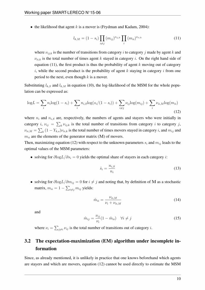
• the likelihood that agent k is a mover is (Frydman and Kadam, 2004):

lk,M = (1− si)∏i 6=j

(mij)νij,k

∏i

(mii)νii,k (11)

where νij,k is the number of transitions from category i to category j made by agent k andνii,k is the total number of times agent k stayed in category i. On the right hand side ofequation (11), the first product is thus the probability of agent k moving out of categoryi, while the second product is the probability of agent k staying in category i from oneperiod to the next, even though k is a mover.

Substituting lk,S and lk,M in equation (10), the log-likelihood of the MSM for the whole popu-lation can be expressed as:

logL =∑i

nilog(1− si) +∑i

ni,Slog(si/(1− si)) +∑i 6=j

νijlog(mij) +∑i

νii,M log(mii)

(12)where ni and ni,S are, respectively, the numbers of agents and stayers who were initially incategory i, νij =

∑k νij,k is the total number of transitions from category i to category j,

νii,M =∑

k (1− Yk,s)νii,k is the total number of times movers stayed in category i, andmij andmii are the elements of the generator matrix (M) of movers.Then, maximizing equation (12) with respect to the unknown parameters si and mij leads to theoptimal values of the MSM parameters:

• solving for ∂logL/∂si = 0 yields the optimal share of stayers in each category i:

si =ni,Sni

(13)

• solving for ∂logL/∂mij = 0 for i 6= j and noting that, by definition of M as a stochasticmatrix, mii = 1−

∑i 6=jmij yields:

mii =νii,M

νi + νii,M(14)

andmij =

νijνi

(1− mii) ∀i 6= j (15)

where νi =∑

j 6=i νij is the total number of transitions out of category i.

3.2 The expectation-maximization (EM) algorithm under incomplete in-formation

Since, as already mentioned, it is unlikely in practice that one knows beforehand which agentsare stayers and which are movers, equation (12) cannot be used directly to estimate the MSM

10


parameters. Indeed, because the transition process is assumed to be a stochastic process, evenmovers may remain for a long time in their initial category before moving, so that they may notappear as movers but as stayers over the observed period. Therefore, Fuchs and Greenhouse(1988) suggested that the MSM parameters could be estimated using the EM algorithm devel-oped by Dempster, Laird, and Rubin (1977): rather than observing the dummy variable Yk,S ,the EM algorithm allows its expected value E(Yk,S) to be estimated, i.e., the probability foreach agent k to be a stayer, given agent k’s initial category and observed transition sequence.Following Frydman and Kadam (2004), the four steps of the EM algorithm are defined in thecase of the MSM as follows.

(i) Initialization: Arbitrarily choose initial values s0i for the shares of stayers and m0ii for the

main diagonal entries of the generator matrix (M) of movers.

(ii) Expectation: At iteration p of the algorithm, compute the probability of observing agentk as generated by a stayer, Ep(Yk,S). If at least one transition is observed for agent k then setEp(Yk,S) = 0, otherwise set it to:

Ep(Yk,S) =spi

spi + (1− spi )(mpii)νii,k

(16.i)

Then compute:

• the expected value of the number of stayers in category i, Ep(ni,S), as:

Ep(ni,S) =∑k

Ep(Yk,S) (16.ii)

• and the expected value of the total number of times movers remain in category i,Ep(νii,M),as:

Ep(νii,M) =∑k

(1− Ep(Yk,S))νii,k (16.iii)

(iii) Maximization: Update spi and mpii as follows:

sp+1i =

Ep(ni,S)

niand mp+1

ii =Ep(νii,M)

νi + Ep(νii,M)(16.iv)

(iv) Iteration: Return to expectation step (ii) using sp+1i andmp+1

ii and iterate until convergence.

When convergence is reached, the optimal values s∗i and m∗ii are considered to be the estimatorssi and mii. Then, mij derives from mii as in equation (15).Following Frydman (2005), the standard errors attached to the MSM parameters can be com-puted directly from the EM equations using the method proposed by Louis (1982) (see ap-pendix). The standard errors attached to the overall 1-year TPM Φ can then be derived applying

11


the standard Delta method to equation (8). Finally, because it is more complicated to apply theDelta method to equation (9) as it involves powers of matrices, we used a bootstrap samplingmethod to compute standard errors attached to the r-step TPMs M(r) and Φ(r) (Efron, 1979;Efron and Tibshirani, 1986).

4 Model comparison

Two types of analysis were performed to assess whether or not the MSM outperforms the MCM.

4.1 Likelihood ratio (LR) test

The likelihood ratio test allows the in-sample performance of the two models in recoveringthe data generating process to be compared. As stated by Frydman and Kadam (2004), thelikelihood ratio statistic for the MSM is given by:

LR =LMCM(Π)

LMSM(S, M)(17)

where LMCM and LMSM are the estimated maximum likelihoods for the MCM and the MSM,respectively. Theoretically, the asymptotic distribution of −2log(LR), under H0, is chi-squarewith (G − 1) × J degrees of freedom. In the case of the MSM, the likelihood ratio tests thehypothesis that the process follows a MCM (H0 : S = 0) against the hypothesis that it is amixture of movers and stayers (H1 : S 6= 0). The observed log-likelihood for both modelscan be derived from equation (10), by imposing Yk,S = 0 for all agents k for the MCM and byreplacing Yk,S by its optimal expected value (E∗(Yk,S)) for the MSM.

4.2 Average Marginal Error (AME)

The estimated parameters were used to compute the corresponding r-step TPMs, i.e., Π(r) =

(Π)r for the MCM and Φ(r) = S + (I− S)(M)r for the MSM. These r-step TPMs were thenused to perform out-of-sample short- to long-run projections of farm distributions across sizecategories according to equation (1) (see below).On the one hand, TPMs from both models were compared to the observed one, providing asecond in-sample assessment complementary to the likelihood ratio test. This comparison wasbased on the average marginal error (AME) defined by Cipollini, Ferretti, and Ganugi (2012)as:

AME =1

J × J∑i,j

√√√√( p(r)ij − p(r)ijp(r)ij

)2

(18)

where p(r)ij and p(r)ij are the predicted and observed TPM entries, respectively:

12


• p(r)ij ≡ π(r)ij under the MCM while p(r)ij ≡ φ

(r)ij under the MSM

• p(r)ij derives from equation (4).

On the other hand, AMEs were similarly computed for both the MCM and MSM projections offarm size distributions with respect to the actually observed ones, providing an out-of-samplecomparison of the models.In contrast to some dissimilarity indexes (Jafry and Schuermann, 2004) or the matrix of resid-uals (Frydman, Kallberg, and Kao, 1985), the AME provides a global view of the distancebetween the predicted TPM or population distribution across size categories and the observedones. It can be interpreted as the average percentage of deviations on predicting the observedTPM or population distribution across size categories. Thus, the higher the AME, the moredifferent the computed TPM or distribution with respect to the observed one. The better modelis therefore the one which yields the lowest AME.

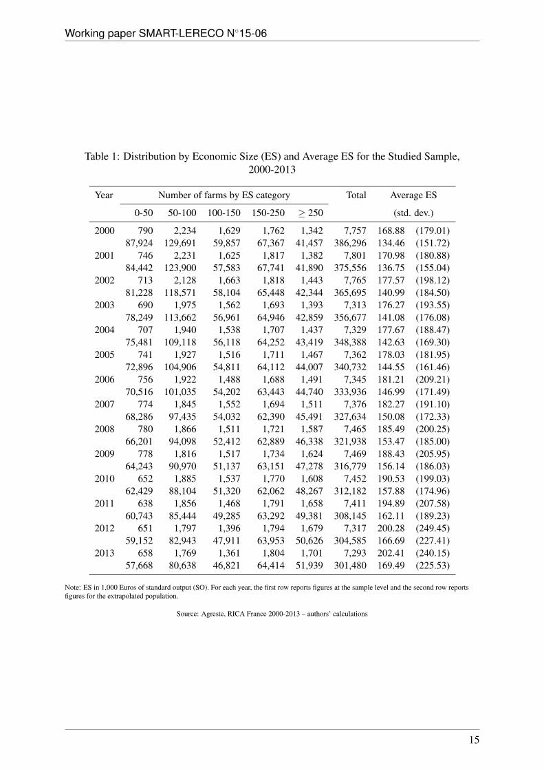
5 Data

In our empirical application, we used the 2000-2013 data of the “Réseau d’Information Compt-able Agricole” (RICA), the French implementation of the Farm Accountancy Data Network(FADN). FADN is an annual survey which is defined at the European Union (EU) level and iscarried out in each member state. The information collected at the individual level relates toboth the physical and structural characteristics of farms and their economic and financial char-acteristics. Note that, to comply with accounting standards which may differ from one countryto the other (e.g., the recording of asset depreciation), the questionnaire defined at the EU levelmay be adapted at the national level, which is the case for France, but this had no consequencesfor our study.In France, RICA is produced and disseminated by the statistical and foresight office of theFrench ministry for agriculture. It focuses on ‘middle and large’ farms (see below) and con-stitutes a stratified and rotating panel of approximately 7,000 farms surveyed each year. Some10% of the sample is renewed every year so that, on average, farms are observed during 5 con-secutive years. However, some farms may be observed only once, and others several, yet notconsecutive, times. Some farms remained in the database over the whole of the studied pe-riod, i.e., fourteen consecutive years. Each farm in the dataset is assigned a weighting factorwhich reflects its stratified sampling probability. These factors allow for extrapolation at thepopulation level.3

As we considered all farms in the sample whatever their type of farming, we chose to con-centrate on size as defined in economic terms. In accordance with the EU regulation (CE)

3To learn more about RICA France, see http://www.agreste.agriculture.gouv.fr/. Thedataset used in this article directly derives from the version of the RICA publicly available at this address. Tolearn more about FADN in general, see http://ec.europa.eu/agriculture/rica/index.cfm.

13

http://www.agreste.agriculture.gouv.fr/

http://ec.europa.eu/agriculture/rica/index.cfm


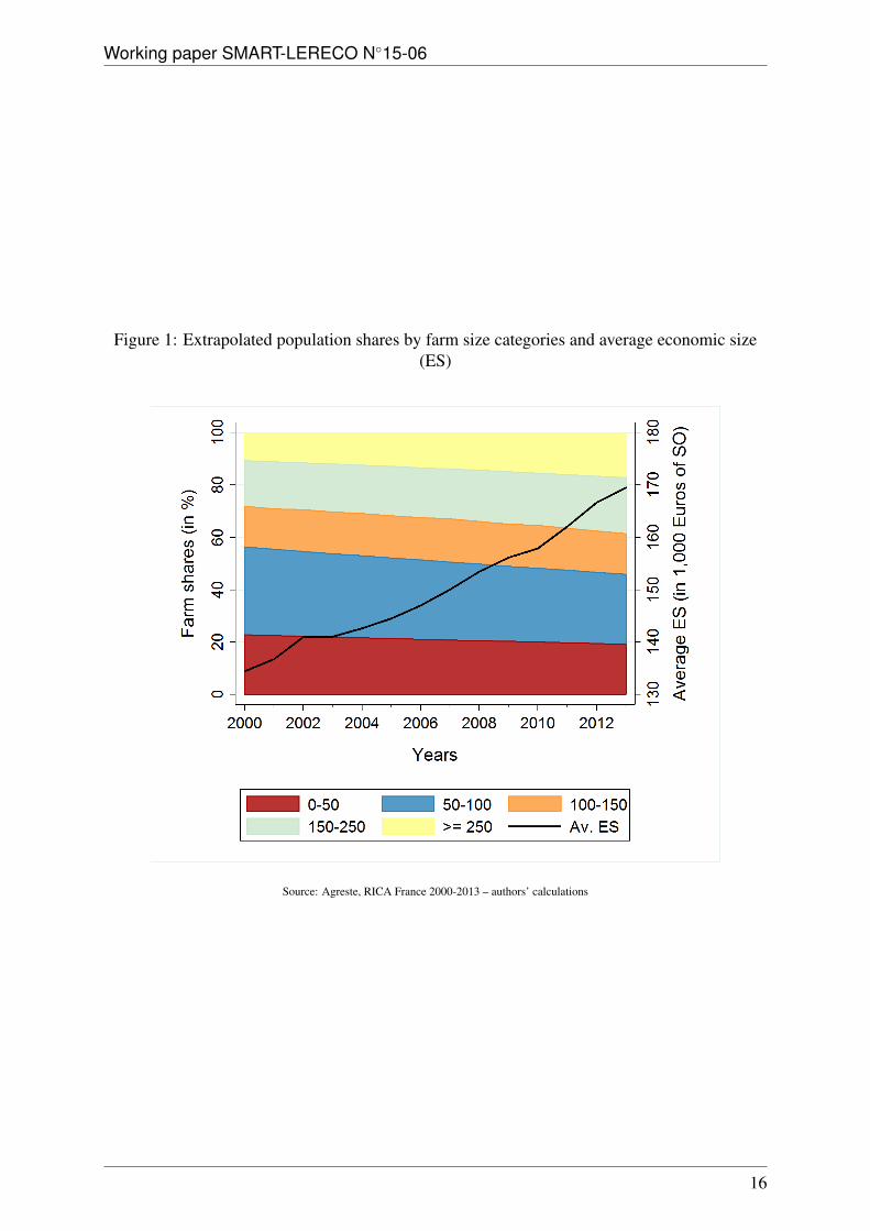
No1242/2008, European farms are classified into fourteen economic size (ES) categories, eval-uated in terms of total standard output (SO) expressed in Euros.4 As mentioned above, inFrance, RICA focuses on ‘medium and large’ farms, those whose SO is greater than or equalto 25,000 Euros; this corresponds to ES category 6 and above. Since size categories are notequally represented in the sample, we aggregated the nine ES categories available in RICA intofive: strictly less than 50,000 Euros of SO (ES6); from 50,000 to less than 100,000 Euros ofSO (ES7); from 100,000 to less than 150,000 Euros of SO (lower part of ES8); from 150,000to less than 250,000 Euros of SO (upper part of ES8); 250,000 Euros of SO and more (ES9 toES14).RICA being a rotating panel, farms which either enter or leave the sample in a given yearcannot be considered as actual entries into or exits from the agricultural sector. Thus, we couldnot work directly on the evolution of farm numbers but rather on the evolution of populationshares by size categories, i.e., the size distribution in the population. Table 1 presents the year-on-year evolution by size categories of farm numbers for the extrapolated population, as wellas the number of farms in the sample. It also reports the average ES in thousand of Euros of SOboth at the sample and extrapolated population levels.Figure 1 shows that the share of smaller farms (below 100,000 Euros of SO) decreased from56% to 46% between 2000-2013 while the share of larger farms (above 150,000 Euros of SO)increased from 28% to 38%, and the share of intermediate farms (100,000 to less than 150,000Euros of SO) remained stable at 16%. As a consequence, as can be seen from table 1 andfigure 1, the average economic size of French farms was multiplied by more than 1.25 overthis period. Note that table 1 also reveals that the size distribution became more heterogeneoussince the standard deviation of the economic size was multiplied by almost 1.5, a feature whichhas already been observed for the population of French farms as a whole and in other periods(Butault and Delame, 2005; Desriers, 2011). Finally, table 1 reveals that these observations alsoapply at the sample level, even though the latter is skewed towards larger sizes with respect tothe population as a whole.In order to assess which model performed better, we compared the MCM and the MSM on thebasis of both in-sample estimation and out-of-sample size distribution forecasts. To do so, wesplit the RICA database into two parts: (i) observations from 2000 to 2010 were used to estimatethe parameters of both models; (ii) observations from 2011 to 2013 were used to compare theactual farm size distributions with their predicted counterparts for both models. Note that, indoing so we assumed that, in the case of the MSM, eleven years is a long enough time intervalto robustly estimate the transition process of movers.

4SO has been used as the measure of economic size since 2010. Before this date, economic size was measuredin terms of standard gross margin (SGM). However, SO calculations have been retropolated for 2000 to 2009,allowing for consistent time series analysis (European Commission, 2010).

14


Table 1: Distribution by Economic Size (ES) and Average ES for the Studied Sample,2000-2013

Year Number of farms by ES category Total Average ES

0-50 50-100 100-150 150-250 ≥ 250 (std. dev.)

2000 790 2,234 1,629 1,762 1,342 7,757 168.88 (179.01)87,924 129,691 59,857 67,367 41,457 386,296 134.46 (151.72)

2001 746 2,231 1,625 1,817 1,382 7,801 170.98 (180.88)84,442 123,900 57,583 67,741 41,890 375,556 136.75 (155.04)

2002 713 2,128 1,663 1,818 1,443 7,765 177.57 (198.12)81,228 118,571 58,104 65,448 42,344 365,695 140.99 (184.50)

2003 690 1,975 1,562 1,693 1,393 7,313 176.27 (193.55)78,249 113,662 56,961 64,946 42,859 356,677 141.08 (176.08)

2004 707 1,940 1,538 1,707 1,437 7,329 177.67 (188.47)75,481 109,118 56,118 64,252 43,419 348,388 142.63 (169.30)

2005 741 1,927 1,516 1,711 1,467 7,362 178.03 (181.95)72,896 104,906 54,811 64,112 44,007 340,732 144.55 (161.46)

2006 756 1,922 1,488 1,688 1,491 7,345 181.21 (209.21)70,516 101,035 54,202 63,443 44,740 333,936 146.99 (171.49)

2007 774 1,845 1,552 1,694 1,511 7,376 182.27 (191.10)68,286 97,435 54,032 62,390 45,491 327,634 150.08 (172.33)

2008 780 1,866 1,511 1,721 1,587 7,465 185.49 (200.25)66,201 94,098 52,412 62,889 46,338 321,938 153.47 (185.00)

2009 778 1,816 1,517 1,734 1,624 7,469 188.43 (205.95)64,243 90,970 51,137 63,151 47,278 316,779 156.14 (186.03)

2010 652 1,885 1,537 1,770 1,608 7,452 190.53 (199.03)62,429 88,104 51,320 62,062 48,267 312,182 157.88 (174.96)

2011 638 1,856 1,468 1,791 1,658 7,411 194.89 (207.58)60,743 85,444 49,285 63,292 49,381 308,145 162.11 (189.23)

2012 651 1,797 1,396 1,794 1,679 7,317 200.28 (249.45)59,152 82,943 47,911 63,953 50,626 304,585 166.69 (227.41)

2013 658 1,769 1,361 1,804 1,701 7,293 202.41 (240.15)57,668 80,638 46,821 64,414 51,939 301,480 169.49 (225.53)

Note: ES in 1,000 Euros of standard output (SO). For each year, the first row reports figures at the sample level and the second row reportsfigures for the extrapolated population.

Source: Agreste, RICA France 2000-2013 – authors’ calculations

15


Figure 1: Extrapolated population shares by farm size categories and average economic size(ES)


16

Working

paperSM

AR

T-LER

EC

ON15-06

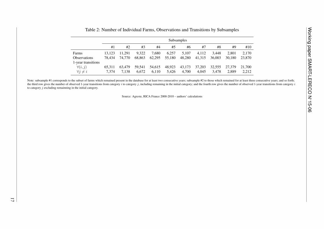
Table 2: Number of Individual Farms, Observations and Transitions by Subsamples

Subsamples

#1 #2 #3 #4 #5 #6 #7 #8 #9 #10

Farms 13,123 11,291 9,322 7,680 6,257 5,107 4,112 3,448 2,801 2,170Observations 78,434 74,770 68,863 62,295 55,180 48,280 41,315 36,003 30,180 23,8701-year transitions∀(i, j) 65,311 63,479 59,541 54,615 48,923 43,173 37,203 32,555 27,379 21,700∀j 6= i 7,374 7,138 6,672 6,110 5,426 4,700 4,045 3,478 2,889 2,212

Note: subsample #1 corresponds to the subset of farms which remained present in the database for at least two consecutive years; subsample #2 to those which remained for at least three consecutive years; and so forth;the third row gives the number of observed 1-year transitions from category i to category j, including remaining in the initial category; and the fourth row gives the number of observed 1-year transitions from category ito category j excluding remainning in the initial category.


17


For in-sample estimations, we also had to restrict the subsample to farms which were presentin the database for at least two consecutive years in order to observe potential transitions. Thecorresponding unbalanced panel then comprised 13,123 farms out of the 17,285 farms in theoriginal database (76%), leading to 78,434 farm×year observations and 65,311 individual 1-year transitions (including staying in the same category) from 2000 to 2010. Furthermore, tensubsamples could be constructed from this unbalanced panel, according to the minimum numberof consecutive years a farm remained present in the database, from two to eleven: subsample#1 thus corresponds to the subset of farms which remained for at least two consecutive years(full 2000-2010 unbalanced panel); subsample #2 to those which remained for at least threeconsecutive years; and so forth, up to subsample #10 which corresponds to the 2000-2010balanced panel. Table 2 reports the corresponding numbers of individual farms and observedtransitions for each subsample.Before proceeding with the results, it should finally be noted that because we had to workwith subsets of the full sample, the transition probabilities reported in the next section can onlybe viewed as conditional on having been observed over a specific number of consecutive yearsduring the whole period under study, and therefore should not be considered to be representativefor the whole population of ‘medium and large’ French farms.

6 Results

In this section, we first report the results of in-sample estimations, i.e., the estimated 1-yearTPMs for the MCM and the MSM. Then we compare the models based on in-sample results inorder to assess which one performs better in recovering the underlying transition process bothfrom a short-run and a long-run perspective. Finally, we compare the models in their ability toforecast future farm size distributions based on out-of-sample observations.

6.1 In-sample estimation results

The MCM and MSM parameters were estimated for each of the ten subsamples described in theprevious section. But because it would take too much space to report the results for all of them,only those for subsample #10 are reported here, that is, using the 2000-2010 balanced panelwhich consists of 2,170 individual farms and 21,700 observed transitions over the 11 years (seelast column of table 2). However, when any of the other subsamples are considered, the results,and hence conclusions, remain very similar to those reported here.5

Table 3 reports the 1-year TPM estimated from subsample #10 under the MCM assumption. As

5Actually, it turned out that considering subsamples which include farms remaining for a shorter period inthe database added noise to the estimation of both models: the less time farms remain in the database, the moreincomplete the information about them, i.e., the more difficult the estimation of their true behavior. Thus, theAMEs were higher with low rank subsamples than with high rank subsamples, subsample #10 eventually yieldingthe lowest AMEs.

18


is usually found in the literature, the matrix is strongly diagonal, meaning that its main diagonalelements exhibit by far the largest values and that probabilities rapidly decrease as we moveaway from the main diagonal. This means that, overall, farms are more likely to remain in theirinitial size category from one year to the next. Note that this does not mean no size change atall but, at least, no change sufficient to move to another category as we defined them.

Table 3: Estimated 1-Year TPM under MCM (Π) (subsample #10)

ES class

0-50 50-100 100-150 150-250 ≥ 250

ES

clas

s

0-50 0.917 0.079 0.002 0.002 0.001(0.024) (0.007) (0.001) (0.001) (0.001)

50-100 0.030 0.898 0.065 0.005 0.002(0.002) (0.013) (0.004) (0.001) (0.001)

100-150 0.002 0.062 0.854 0.080 0.002(0.001) (0.004) (0.014) (0.004) (0.001)

150-250 0.001 0.004 0.054 0.886 0.055(0.000) (0.001) (0.003) (0.012) (0.003)

≥ 250 0.000 0.001 0.003 0.048 0.948(0.000) (0.001) (0.001) (0.003) (0.014)

Log-likelihood: logLMCM = −8, 689.36Note: estimated parameters in bold font, standard errors in parentheses.


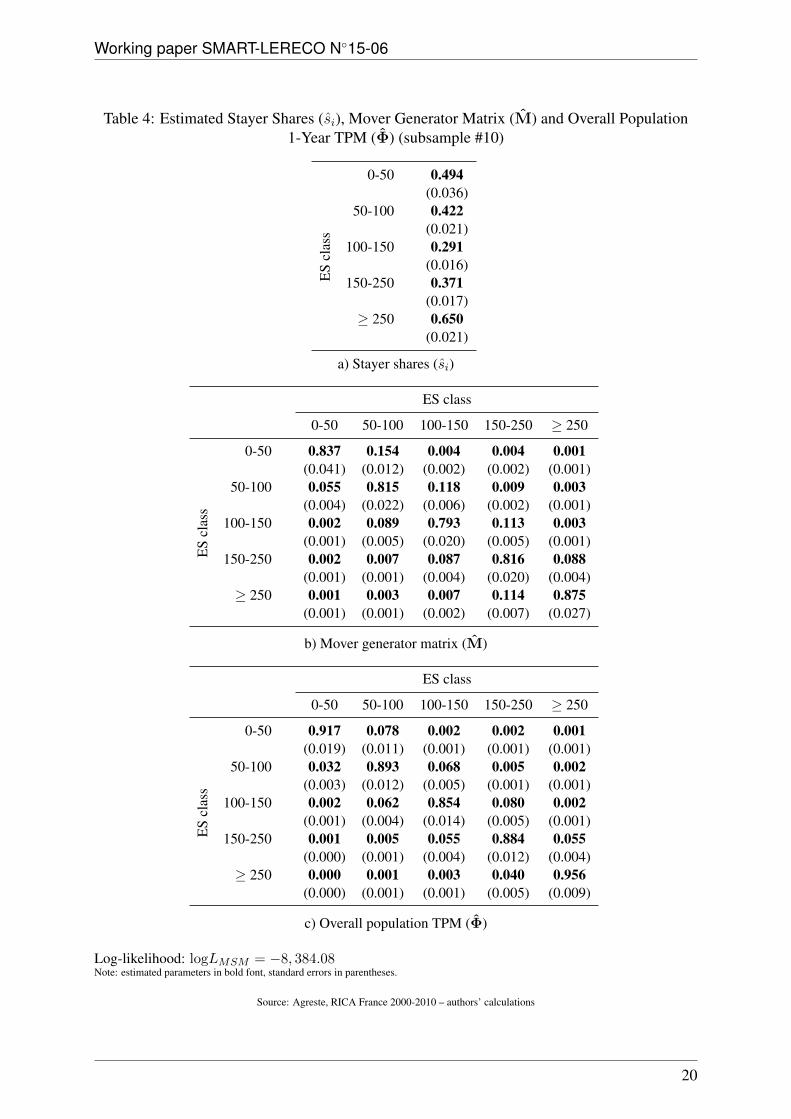
Table 4 reports the estimated shares of stayers and generator matrix of movers along with thecorresponding 1-year TPM for the whole population under the MSM assumption, and also forsubsample #10. Two main results can be drawn from this table. First, the estimated stayer shares(panel a of table 4) show that the probability of being a stayer is close to or above 30% whateverthe category considered; it reaches almost 50% for farms below 50,000 Euros of SO and is evenhigher than 60% for farms over 250,000 Euros of SO. This means that, according to the MSMand depending on the size category, at least 30% of the farms are likely to remain in their initialcategory for at least 10 more years. Second, the generator matrix (panel b of table 4) revealsthat even though movers are by definition expected to transit from one category to another inthe next ten years, yet the highest probability for them is to remain in the same category fromone year to the next. Since the average time spent by movers in a particular category is givenby 1/(1 −mii) (see appendix), it can be seen from table 4 that movers in the intermadiate ESclass (1/(1 − 0.793) = 4.8) were likely to remain in the same category for almost five years,while those above 250,000 Euros of SO (1/(1 − 0.875) = 8) were likely to remain for eightyears before moving. In other words, farms which remained in a particular category for quitea long time (theoretically even over the whole observation period) were not necessarily stayersbut may well be movers who had not yet moved. Altogether, these two results yield a 1-year

19


Table 4: Estimated Stayer Shares (si), Mover Generator Matrix (M) and Overall Population1-Year TPM (Φ) (subsample #10)

ES

clas

s

0-50 0.494(0.036)

50-100 0.422(0.021)

100-150 0.291(0.016)

150-250 0.371(0.017)

≥ 250 0.650(0.021)

a) Stayer shares (si)

ES class

0-50 50-100 100-150 150-250 ≥ 250

ES

clas

s

0-50 0.837 0.154 0.004 0.004 0.001(0.041) (0.012) (0.002) (0.002) (0.001)

50-100 0.055 0.815 0.118 0.009 0.003(0.004) (0.022) (0.006) (0.002) (0.001)

100-150 0.002 0.089 0.793 0.113 0.003(0.001) (0.005) (0.020) (0.005) (0.001)

150-250 0.002 0.007 0.087 0.816 0.088(0.001) (0.001) (0.004) (0.020) (0.004)

≥ 250 0.001 0.003 0.007 0.114 0.875(0.001) (0.001) (0.002) (0.007) (0.027)

b) Mover generator matrix (M)

ES class

0-50 50-100 100-150 150-250 ≥ 250

ES

clas

s

0-50 0.917 0.078 0.002 0.002 0.001(0.019) (0.011) (0.001) (0.001) (0.001)

50-100 0.032 0.893 0.068 0.005 0.002(0.003) (0.012) (0.005) (0.001) (0.001)

100-150 0.002 0.062 0.854 0.080 0.002(0.001) (0.004) (0.014) (0.005) (0.001)

150-250 0.001 0.005 0.055 0.884 0.055(0.000) (0.001) (0.004) (0.012) (0.004)

≥ 250 0.000 0.001 0.003 0.040 0.956(0.000) (0.001) (0.001) (0.005) (0.009)

c) Overall population TPM (Φ)

Log-likelihood: logLMSM = −8, 384.08Note: estimated parameters in bold font, standard errors in parentheses.


20


TPM for the whole population which is also highly diagonal (panel c of table 4).

6.2 In-sample model comparison

Both models are in agreement in estimating that, at the overall population level, farms weremore likely to remain in their initial size category from year to year, confirming that structuralchange in the agricultural sector is a slow process which needs to be investigated in the long-run. In this respect, while the 1-year TPMs look very similar across both models, the resultinglong-run transition model differs between the MCM, given by equation (5), and the MSM, givenby equation (9). It is therefore important to assess which model performs better in recoveringthe true underlying transition process.The first assessment method used, namely the likelihood ratio test, reveals that the MSMyields a better fit than the MCM: the value of the test statistic as defined by equation (17) is−2log(LR) = −2 × (−8, 689.36 + 8, 384.08) = 610.56, which is highly significant since thecritical value of a chi-square distribution with (G− 1)× J = 5 degrees of freedom and the 1%significance level is χ2

0.99(5) = 15.09. This leads to the rejection of the H0 assumption that thestayer shares are all zero, and thus to the conclusion that the MSM allows the data generatingprocess to be recovered in a more efficient way than the MCM. The MSM should therefore alsolead to a better approximation of transition probabilities in the long-run.The second assessment method used allows this very point to be assessed. Estimated parametersfor both models were used to derive the corresponding 10-year TPMs, namely Π(10) = (Π)10

for the MCM and Φ(10) = S + (I− S)(M)10 for the MSM. These estimated long-run matri-ces were then compared to the observed one, P(10), which is derived from equation (4) andsubsample #10. It appears from visual inspection of the three corresponding panels of table 5that the MSM 10-year matrix more closely resembles the actually observed one than the MCM10-year matrix. In particular, we find as expected that the diagonal elements of Π(10) largelyunderestimate those of P(10) while those of Φ(10) are much closer. This means that the MCMlargely tends overestimate the mobility of farms in the long-run, with respect to the MSM. TheAMEs reported in table 6 confirm the superiority of the MSM over the MCM in modeling thelong-run transition process. The AME for the overall predicted 10-year TPM is around 0.95 forthe MCM while it is about 0.78 for the MSM. This means that the MSM is about 17 percentagepoints closer to the observed TPM than the MCM in the long-run. However, the AMEs alsoconfirm that the improvement comes mainly from the main diagonal elements: when only theseare considered, the MSM performs about five times better than the MCM (0.292/0.057 = 5.1),while both models are almost comparable for off-diagonal elements, with the MCM this timeperforming slightly better (0.657/0.724 = 0.9).Finally, table 5 also shows that the standard errors associated with the elements of the esti-mated matrices, computed using a standard bootstrapping method with 1,000 replications, aresystematically higher with the MCM than with the MSM; the MSM estimator is thus also more

21


Table 5: Observed 10-Year TPM and Predicted 10-Year TPMs for both Models (subsample#10).

ES class

0-50 50-100 100-150 150-250 ≥ 250E

Scl

ass

0-50 0.715 0.235 0.029 0.014 0.00750-100 0.107 0.641 0.199 0.038 0.015

100-150 0.020 0.146 0.536 0.268 0.030150-250 0.010 0.032 0.096 0.630 0.232≥ 250 0.005 0.021 0.020 0.124 0.830

a) Observed 10-year TPM (P(10))

ES class

0-50 50-100 100-150 150-250 ≥ 250

ES

clas

s

0-50 0.476 0.361 0.106 0.043 0.014(0.028) (0.020) (0.008) (0.006) (0.004)

50-100 0.141 0.467 0.240 0.116 0.036(0.011) (0.015) (0.011) (0.007) (0.004)

100-150 0.044 0.234 0.338 0.281 0.103(0.004) (0.011) (0.013) (0.011) (0.007)

150-250 0.015 0.082 0.193 0.428 0.282(0.002) (0.005) (0.010) (0.013) (0.013)

≥ 250 0.005 0.026 0.068 0.245 0.656(0.001) (0.003) (0.005) (0.013) (0.018)

b) MCM predicted 10-year TPM (Π(10))

ES class

0-50 50-100 100-150 150-250 ≥ 250

ES

clas

s

0-50 0.690 0.140 0.097 0.053 0.020(0.017) (0.010) (0.007) (0.005) (0.003)

50-100 0.060 0.684 0.126 0.090 0.040(0.007) (0.010) (0.007) (0.005) (0.003)

100-150 0.041 0.119 0.586 0.164 0.090(0.004) (0.007) (0.012) (0.009) (0.006)

150-250 0.018 0.062 0.117 0.676 0.127(0.002) (0.004) (0.006) (0.010) (0.009)

≥ 250 0.005 0.021 0.048 0.093 0.833(0.001) (0.002) (0.003) (0.005) (0.008)

c) MSM predicted 10-year TPM (Φ(10))

Note: estimated parameters in bold font, bootstrap standard errors in parentheses (1,000 replications).


22


Table 6: Average Marginal Error (AME) between the Predicted 10-year TPMs (Π(10) andΦ(10)) and the Observed TPM (P(10)) (subsample #10)

Model Overall Main diagonal Off-diagonalmatrix elements elements

MCM 0.949 0.292 0.657(0.044) (0.010) (0.036)

MSM 0.781 0.057 0.724(0.034) (0.007) (0.035)

Note: bootstrap standard errors in parenthesss (1,000 replications).


efficient (in the econometric sense) than the MCM one in recovering the underlying transitionprocess.

6.3 Out-of-sample projections

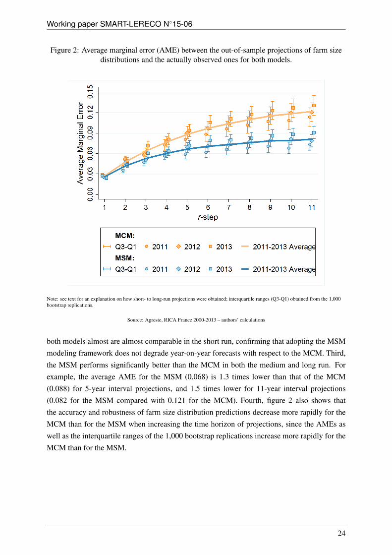
In-sample estimation results lead us to conclude that accounting for unobserved heterogeneityin the rate of movement of farms, as the MSM does, avoids overestimating their mobility acrosssize categories. The MSM should therefore also lead to a more accurate prediction of the sizedistribution of farms in the long run, without hampering that in the short run.To validate this point, we performed out-of-sample short- to long-run projections of the distri-bution of farm sizes using the parameters for both models as estimated with subsample #10. Todo so, farm size distributions in 2011, 2012 and 2013 were predicted from a short- to long-runperspective, by applying the estimated r-step TPMs (for 1 ≤ r ≤ 11) to the correspondingobserved distributions from 2000 to 2012. In other words, distributions in 2011, 2012 and2013 were predicted: by applying the estimated 1-year TPMs (Π for the MCM and Φ forthe MSM) to the observed distributions in 2010, 2011 and 2012, respectively; by applying theestimated 2-year TPMs (Π(2) = (Π)2 for the MCM and Φ(2) = S + (I − S)(M)2 for theMSM) to the observed distributions in 2009, 2010 and 2011, respectively; and so forth. Thisprocess was continued by applying the estimated r-step TPMs (Π(r) = (Π)r for the MCM andΦ(r) = S + (I− S)(M)r for the MSM) to the observed distributions in (2011− r), (2012− r)and (2013 − r) and varying r up to eleven. Then, the resulting distributions for both modelswere compared to the actually observed distributions in 2011, 2012 and 2013 (see table 1). Thecorresponding AMEs reported in figure 2 summarize the results obtained for the 1,000 bootstrapreplications.Four conclusions can be drawn from figure 2. First, as expected, the accuracy of both modelsdecreases when increasing the time horizon of projection: the computed AMEs are significantlysmaller in the short run than they are in the medium and long run for both models. Second,

23


Figure 2: Average marginal error (AME) between the out-of-sample projections of farm sizedistributions and the actually observed ones for both models.

Note: see text for an explanation on how short- to long-run projections were obtained; interquartile ranges (Q3-Q1) obtained from the 1,000bootstrap replications.


both models almost are almost comparable in the short run, confirming that adopting the MSMmodeling framework does not degrade year-on-year forecasts with respect to the MCM. Third,the MSM performs significantly better than the MCM in both the medium and long run. Forexample, the average AME for the MSM (0.068) is 1.3 times lower than that of the MCM(0.088) for 5-year interval projections, and 1.5 times lower for 11-year interval projections(0.082 for the MSM compared with 0.121 for the MCM). Fourth, figure 2 also shows thatthe accuracy and robustness of farm size distribution predictions decrease more rapidly for theMCM than for the MSM when increasing the time horizon of projections, since the AMEs aswell as the interquartile ranges of the 1,000 bootstrap replications increase more rapidly for theMCM than for the MSM.

24


7 Concluding remarks

The modeling framework implemented here, namely the mover-stayer model (MSM), is moregeneral than the simple Markov chain model (MCM) since it accounts for unobserved hetero-geneity in the rate of movement of farms. Within this extended framework, the 1-year transitionprobability matrix is decomposed into a fraction of ‘stayers’ who remain in their initial sizecategory and a fraction of ‘movers’ who follow a standard Markovian process. To estimatethe model, we improved Blumen, Kogan, and McCarthy (1955)’s calibration method by usingthe elaborate expectation-maximization (EM algorithm) estimation method proposed by Fry-dman (2005) in order to account for incomplete information. Finally, we computed standarderrors for long-run matrices and farm size distributions using a bootstrap method, with 1,000replications of each estimation and projection. This allowed the models to be compared in astatistically robust manner, which adds to the existing literature. Our results show that, withrespect to the MCM, accounting for unobserved farm heterogeneity enables closer estimates ofboth the observed transition matrix and the distribution of farms across size categories in thelong-run to be derived, without degrading any short-run analysis. This result is consistent withthe findings in other strands of the economic literature, namely that, by relaxing the assumptionof homogeneity in the transition process which is the basis of the MCM, the MSM leads to abetter representation of the underlying structural change process.However, this modeling framework remains quite a restricted and simplified version of the moregeneral model, the mixed-Markov chain model (M-MCM), which we presented as an introduc-tion to the MSM. Extending the MSM further could therefore lead to even more economicallysound, as well as statistically more accurate, models for the farming sector. We briefly men-tion some of such extensions which we think are promising. Firstly, more heterogeneity acrossfarms could be incorporated by allowing for more than two unobserved types. For example,accounting for different types of movers could yield a better representation of the structuralchange process in the farming sector by allowing farms which tend mainly to enlarge to be dis-entangled from farms which tend mainly to shrink. Secondly, the quite strong assumption of a‘pure stayer’ type could be relaxed because it may look unlikely that some farms ‘never move atall’, i.e., will not change size category over their entire lifespan. In this respect, the robustnessof the MSM to the number of years during which farms are observed could be investigated. In-deed, considering eleven years to perform in-sample estimations, our results show that moversmay stay five to eight years in a given category before experiencing a large enough (positive ornegative) size change to reach another category. We can then infer that the shorter the observa-tion period, the higher the number of farms which would be inappropriately considered as ‘purestayers’. From a methodological point of view, this leads to the conclusion that long enoughpanel data needs to be available if the MSM is to be empirically implemented. This could beseen as a shortcoming of the MSM with respect to the MCM but it is in fact consistent withfarm structural change being a long-run and slow process.

25


Our final recommendation is that the proposed modeling framework should be extended toaccount for entries and exits and that a non-stationary version of the M-MCM model shouldbe developed. Since this should allow the transition process to be recovered in an even moreefficient way, it would surely prove to be very insightful for analyzing the factors which drivestructural change in the farming sector, including agricultural policies, not only from a sizedistribution perspective, but also as regards the evolution of farm numbers.

Acknowledgments

Legrand D.F. Saint-Cyr benefits from a research grant from Crédit Agricole en Bretagne in theframework of the chair "‘Enterprises and Agricultural Economics"’ created in partnership withAgrocampus Ouest.

References

Anderson, T.W., and L.A. Goodman. 1957. “Statistical Inference about Markov Chains.” Annals

of Mathematical Statistics 28:89–110.

Blumen, I., M. Kogan, and P.J. McCarthy. 1955. The industrial mobility of labor as a probability

process, vol. VI. Cornell Studies in Industrial and Labor Relations.

Butault, J.P., and N. Delame. 2005. “Concentration de la production agricole et croissance desexploitations.” Economie et statistique 390:47–64.

Cipollini, F., C. Ferretti, and P. Ganugi. 2012. “Firm size dynamics in an industrial district: Themover-stayer model in action.” In A. Di Ciaccio, M. Coli, and J. M. Angulo Ibanez, eds. Ad-

vanced Statistical Methods for the Analysis of Large Data-Sets. Springer Berlin Heidelberg,pp. 443–452.

Dempster, A.P., N.M. Laird, and D.B. Rubin. 1977. “Maximum likelihood from incompletedata via the EM algorithm.” Journal of the Royal Statistical Society 39:1–38.

Desriers, M. 2011. “Farm structure. Agricultural census 2010. Production is concentrated inspecialised farms.” Agreste: la statistique agricole, Agreste Primeur 272.

Dutta, J., J.A. Sefton, and M.R. Weale. 2001. “Income distribution and income dynamics in theUnited Kingdom.” Journal of Applied Econometrics 16:599–617.

Efron, B. 1979. “Bootstrap methods: Another look at the jackknife.” The Annals of Statistics

7:1–26.

Efron, B., and R. Tibshirani. 1986. “Bootstrap methods for standard errors, confidence intervals,and other measures of statistical accuracy.” Statistical Science 1:54–75.

26


European Commission. 2010. Farm Accounting Data Network. An A to Z of methodology. Brus-sels (Belgium): DG Agri.

Fougère, D., and T. Kamionka. 2003. “Bayesian inference for the mover-stayer model in con-tinuous time with an application to labour market transition data.” Journal of Applied Econo-

metrics 18:697–723.

Frydman, H. 2005. “Estimation in the mixture of Markov chains moving with different speeds.”Journal of the American Statistical Association 100:1046–1053.

—. 1984. “Maximum likelihood estimation in the mover-stayer model.” Journal of the American

Statistical Association 79:632–638.

Frydman, H., and A. Kadam. 2004. “Estimation in the continuous time mover-stayer modelwith an application to bond ratings migration.” Applied Stochastic Models in Business and

Industry 20:155–170.

Frydman, H., J.G. Kallberg, and D.L. Kao. 1985. “Testing the adequacy of Markov chain andmover-stayer models as representations of credit behavior.” Operations Research 33:1203–1214.

Frydman, H., and T. Schuermann. 2008. “Credit rating dynamics and Markov mixture models.”Journal of Banking and Finance 32:1062–1075.

Fuchs, C., and J.B. Greenhouse. 1988. “The EM algorithm for maximum likelihood estimationin the mover-stayer model.” Biometrics 44:605–613.

Goodman, L.A. 1961. “Statistical methods for the mover-stayer model.” Journal of the Ameri-

can Statistical Association 56:841–868.

Hallberg, M.C. 1969. “Projecting the size distribution of agricultural firms. An application of aMarkov process with non-stationary transition probabilities.” American Journal of Agricul-

tural Economics 51:289–302.

Huettel, S., and R. Jongeneel. 2011. “How has the EU milk quota affected patterns of herd-sizechange?” European Review of Agricultural Economics 38:497–527.

Jafry, Y., and T. Schuermann. 2004. “Measurement, estimation and comparison of credit migra-tion matrices.” Journal of Banking & Finance 28:2603–2639.

Karantininis, K. 2002. “Information-based estimators for the non-stationary transition probabil-ity matrix: An application to the Danish pork industry.” Journal of Econometrics 107:275–290.

27


Langeheine, R., and F. Van de Pol. 2002. Applied latent class analysis, Cambridge UniversityPress, chap. Latent markov chains. pp. 304–341.

Lee, T., G. Judge, and A. Zellner. 1977. Estimating the parameters of the Markov probability

model from aggregate time series data. Amsterdam: North Holland.

Lee, T.C., G.G. Judge, and T. Takayama. 1965. “On estimating the transition probabilities of aMarkov process.” Journal of Farm Economics 47:742–762.

Louis, T.A. 1982. “Finding the observed information matrix when using the EM algorithm.”Journal of the Royal Statistical Society. Series B (Methodological) 44:226–233.

MacRae, E.C. 1977. “Estimation of time-varying Markov processes with aggregate data.”Econometrica 45:183–198.

McLachlan, G., and T. Krishnan. 2007. The EM algorithm and extensions, vol. 382. John Wiley& Sons.

Morgan, T.M., C.S. Aneshensel, and V.A. Clark. 1983. “Parameter estimation for mover-stayermodels analyzing depression over time.” Sociological Methods & Research 11:345–366.

Piet, L. 2011. “Assessing structural change in agriculture with a parametric Markov chainmodel. Illustrative applications to EU-15 and the USA.” Paper presented at the XIIIthCongress of the European Association of Agricultural Economist, Zurich (Switzerland).

Spilerman, S. 1972. “The analysis of mobility processes by the introduction of independentvariables into a Markov chain.” American Sociological Review 37:277–294.

Stavins, R.N., and B.F. Stanton. 1980. Alternative procedures for estimating the size distribution

of farms. Department of Agricultural Economics, New York State College of Agriculture andLife Sciences.

Storm, H., T. Heckelei, and R.C. Mittelhammer. 2011. “Bayesian estimation of non-stationaryMarkov models combining micro and macro data.” Discussion Paper No. 2011:2, Universityof Bonn, Institute for Food and Resource Economics, Bonn (Germany).

Weiss, C.R. 1999. “Farm growth and survival: econometric evidence for individual farms inupper Austria.” American Journal of Agricultural Economics 81:103–116.

Zepeda, L. 1995. “Asymmetry and nonstationarity in the farm size distribution of Wiscon-sin milk producers: An aggregate analysis.” American Journal of Agricultural Economics

77:837–852.

Zimmermann, A., and T. Heckelei. 2012. “Structural change of European dairy farms: A cross-regional analysis.” Journal of Agricultural Economics 63:576–603.

28


Zimmermann, A., T. Heckelei, and I.P. Dominguez. 2009. “Modelling farm structural changefor integrated ex-ante assessment: Review of methods and determinants.” Environmental Sci-

ence and Policy 12:601–618.

A Appendix

A.1 Frydman (2005)’s specification of the mixed Markov chain model (M-MCM)

Recall that the general form of the M-MCM is given by equation (6):

Φ = φij =G∑g=1

SgMg (19)

where Mg = mij,g is the TPM defining the 1-step Markov process followed by type-g agents,and Sg = diag(si,g) is a diagonal matrix which gathers the shares of type-g agents in eachcategory.Assuming that all type g TPMs are related to a specific one, arbitrarily chosen as that of the lasttype G, Frydman (2005) gives the TPM of any type g as:

Mg = I−Λg + ΛgM for 1 ≤ g ≤ G− 1 (20)

where I is the J × J identity matrix, Λg = diag(λi,g) and M = MG (i.e., ΛG = I), subjectto 0 ≤ λi,g ≤ 1

1−mii(∀i ∈ J) and 0 ≤ mii ≤ 1, where mii are the main diagonal elements of

matrix M.Within this specification, the λi,g parameters give information about heterogeneity in the ratesof movement across homogeneous agent types:

• λi,g = 0 if type-g agents originally in category i never move out of i;

• 0 < λi,g < 1 if type-g agents originally in category i move at a lower rate than thegenerator matrix M;

• λi,g > 1 if type-g agents originally in category i move at a higher rate than the generatormatrix M.

Then the expected time spent in category i by type-g agents is given by 1(λi,g(1−mii))

(∀λi,g > 0).

29


A.2 Maximum likelihood estimation of the mixed Markov chain model(M-MCM)

Consider that each agent k is observed at some discrete time points in the time interval [0, Tk]with Tk ≤ T , where T is the time horizon of all observations. According to Anderson andGoodman (1957), the likelihood that the transition sequence of agent k (Xk) was generated bythe specific type-g Markov chain (i.e., that k belongs to type g), conditional on knowing that kwas initially in state i, is given by:

lk,g = si,g∏i 6=j

(mij,g)νij,k

∏i

(mii,g)νii,k (21)

where si,g is the share of type-g agents initially in category i, νij,k is the number of transitionsfrom i to j made by agent k (with j 6= i), νii,k is the total time spent by k in category i, andmii,g and mij,g are the elements of Mg.Under Frydman (2005)’s specification of the M-MCM as defined by equation (20) the abovelikelihood can be rewritten as:

lk,g = si,g∏i 6=j

(λi,gmij)νij,k

∏i

(1− λi,g + λi,gmii)νii,k (22)

where λi,g is the relative rate of movement of type-g agents.Then, the log-likelihood function for the whole population is:

logL =N∑k=1

G∑g=1

(Yk,gloglk,g) (23)

where Yk,g is an indicator variable which equals 1 if agent k belongs to type g and 0 otherwise.Note that the log-likelihoods of the MCM and MSM can easily be derived from equation (23)by stating, respectively, G=1 and λi,1 = 1 for the MCM and G=2, λi,1 = 0 and λi,2 = 1 for theMSM.The maximum likelihood estimators, si,g, λi,g, mii and mij , are obtained using the EM algorithmin a similar way to that described in the main text.

A.3 Computing standard errors from EM algorithm equations

Two components are required to compute standard errors from the EM algorithm equations(Louis, 1982): (i) the observed information matrix given by the negative of the Hessian matrix ofthe log-likelihood function and; (ii) the missing information matrix obtained from the gradientvector, that is, the vector of score statistics based on complete information. Since the log-likelihood function given by equation (12) is twice differentiable with respect to the modelparameters, the standard errors can be computed as follows.

30


Let Ωc(z; si, mij) and Ωm(z; si, mij) (i, j = 1, ..., J) be the observed (d × d) information ma-trices in terms of complete and missing information, respectively, where Zk = (Xk, Yk) gathersthe transition sequenceXk of agent k and the unobserved agent’s type dummy variable Yk, and dis the number of estimated parameters. The observed information matrix in terms of incompleteinformation can then be derived as:

Ω(x; si, mij) = Ωc(z; si, mij)−Ωm(z; si, mij) (24)

where Ωm(z; si, mij) is given by:

Ωm(z; si, mij) = E[sc(z; si, mij)× sc(z; si, mij)′] (25)

where sc(z; si, mij) is the vector of score statistics in terms of complete information.Therefore, if the observed information matrix in terms of incomplete information just described,Ω(x; si, mij), is invertible, the standard errors are given by:

se = √ψll (26)

where se is the 1× d vector of standard errors, Ψ = ψll′ = Ω−1(x; si, mij) is defined as theasymptotic covariance matrix of the maximum likelihood estimators si and mij (∀i, j = 1, ..., J)under incomplete information, and l, l′ = 1, ..., d (McLachlan and Krishnan, 2007).

31


Les Working Papers SMART – LERECO sont produits par l’UMR SMART et l’UR LERECO

• UMR SMART L’Unité Mixte de Recherche (UMR 1302) Structures et Marchés Agricoles, Ressources et Territoires comprend l’unité de recherche d’Economie et Sociologie Rurales de l’INRA de Rennes et les membres de l’UP Rennes du département d’Economie Gestion Société d’Agrocampus Ouest. Adresse : UMR SMART - INRA, 4 allée Bobierre, CS 61103, 35011 Rennes cedex UMR SMART - Agrocampus, 65 rue de Saint Brieuc, CS 84215, 35042 Rennes cedex

• LERECO Unité de Recherche Laboratoire d’Etudes et de Recherches en Economie Adresse : LERECO, INRA, Rue de la Géraudière, BP 71627 44316 Nantes Cedex 03 Site internet commun : http://www.rennes.inra.fr/smart

Liste complète des Working Papers SMART – LERECO : http://www.rennes.inra.fr/smart/Working-Papers-Smart-Lereco

http://ideas.repec.org/s/rae/wpaper.html

The Working Papers SMART – LERECO are produced by UMR SMART and UR LERECO

• UMR SMART The « Mixed Unit of Research » (UMR1302) Structures and Markets in Agriculture, Resources and Territories, is composed of the research unit of Rural Economics and Sociology of INRA Rennes and of the members of the Agrocampus Ouest’s Department of Economics Management Society who are located in Rennes. Address: UMR SMART - INRA, 4 allée Bobierre, CS 61103, 35011 Rennes cedex, France UMR SMART - Agrocampus, 65 rue de Saint Brieuc, CS 84215, 35042 Rennes cedex, France

• LERECO Research Unit Economic Studies and Research Lab Address: LERECO, INRA, Rue de la Géraudière, BP 71627 44316 Nantes Cedex 03, France Common website: http://www.rennes.inra.fr/smart_eng/

Full list of the Working Papers SMART – LERECO:

http://www.rennes.inra.fr/smart_eng/Working-Papers-Smart-Lereco http://ideas.repec.org/s/rae/wpaper.html

Contact Working Papers SMART – LERECO INRA, UMR SMART 4 allée Adolphe Bobierre, CS 61103 35011 Rennes cedex, France Email : [email protected]

mailto:[email protected]


2015

Working Papers SMART – LERECO

UMR INRA-Agrocampus Ouest SMART (Structures et Marchés Agricoles, Ressources et Territoires)

UR INRA LERECO (Laboratoire d’Etudes et de Recherches en Economie)

Rennes, France

Date post:	14-Sep-2018
Category:	Documents
Upload:	ngoanh
View:	214 times
Download:	0 times

Movers and stayers in the farming sector: accounting for...

Documents