Eurographics Symposium on Geometry Processing 2010 Olga Sorkine and Bruno Lévy (Guest Editors) Volume 29 (2010), Number 5 Moving Least Squares Coordinates Josiah Manson, Scott Schaefer Texas A&M University Abstract We propose a new family of barycentric coordinates that have closed-forms for arbitrary 2D polygons. These coordinates are easy to compute and have linear precision even for open polygons. Not only do these coordinates have linear precision, but we can create coordinates that reproduce polynomials of a set degree m as long as degree m polynomials are specified along the boundary of the polygon. We also show how to extend these coordinates to interpolate derivatives specified on the boundary. Categories and Subject Descriptors (according to ACM CCS): I.3.5 [Computer Graphics]: Computational Geometry and Object Modeling—Boundary representations 1. Introduction Barycentric coordinates are a standard interpolation tech- nique in Computer Graphics. These coordinates solve a boundary value interpolation problem and can be used to in- terpolate discrete scalar fields, vector fields or even multidi- mensional fields over irregular tessellations. While barycen- tric coordinates were first generalized for Finite Element Analysis [Wac75], the Graphics community has made heavy use of these coordinates for applications such as texture mapping [DMA02], polygon shading [HF06], spline sur- faces [LD89] and surface deformation [JSW05]. Suppose p i ∈ R 2 for i = 1 ... n are the vertices of a poly- gon. These points define a piecewise polynomial boundary curve P i (t ) such that P i (t )=(1 - t ) p i + tp i+1 . Furthermore, assume that each edge of this polygon has an associated function F i (t ) ∈ R. We define a barycentric interpolant of this function as ˆ F (x)= n ∑ i=1 Z 1 0 B i (x, t )F i (t )dt where B i (x, t ) is the barycentric coordinate function associ- ated with the i th edge at parameter t and x ∈ R 2 is a point in the domain. If F i (t )=(1 - t ) f i + tf i+1 , then the interpolant takes on the more familiar form, ˆ F (x)= n ∑ i=1 b i (x) f i where b i (x)= R 1 0 (1 - t )B i (x, t )+ tB i-1 (x, t )dt are the barycentric coordinates of x with respect to the vertices p i . For b i (x) to be barycentric, several properties must hold. First, barycentric coordinates should produce an interpolant that takes on the value of F i (t ) along the boundary. There- fore, ˆ F (P i (t )) = F i (t ). Second, the coordinates should have linear precision. This means that, for all linear L(x), L(x)= n ∑ i=1 Z 1 0 B i (x, t )L(P i (t ))dt . Note that if the coordinates have linear precision, they also form a partition of unity (∑ n i=1 R 1 0 B i (x, t )dt = 1). This prop- erty trivially follows from linear precision if L(x)= 1. While these properties are necessary for B i (x, t ) to be barycentric, we typically require that B i (x, t ) is also smooth in practice. 1.1. Related Work Barycentric coordinates were originally described by Möbius for simplices such as triangles in 2D [Möb27]. While barycentric coordinates are unique for triangles, there are many possible solutions for polygons with more sides. Wachspress extended the idea of barycentric basis function to convex polygons [Wac75] for use in finite element analy- sis, but Wachspress coordinates become undefined over the c 2010 The Author(s) Journal compilation c 2010 The Eurographics Association and Blackwell Publishing Ltd. Published by Blackwell Publishing, 9600 Garsington Road, Oxford OX4 2DQ, UK and 350 Main Street, Malden, MA 02148, USA.
Transcript
Eurographics Symposium on Geometry Processing 2010Olga Sorkine and Bruno Lévy(Guest Editors)
Volume 29 (2010), Number 5
Moving Least Squares Coordinates
Josiah Manson, Scott Schaefer
Texas A&M University
Abstract
We propose a new family of barycentric coordinates that have closed-forms for arbitrary 2D polygons. Thesecoordinates are easy to compute and have linear precision even for open polygons. Not only do these coordinateshave linear precision, but we can create coordinates that reproduce polynomials of a set degree m as long as degreem polynomials are specified along the boundary of the polygon. We also show how to extend these coordinates tointerpolate derivatives specified on the boundary.
Categories and Subject Descriptors (according to ACM CCS): I.3.5 [Computer Graphics]: Computational Geometryand Object Modeling—Boundary representations
1. Introduction
Barycentric coordinates are a standard interpolation tech-nique in Computer Graphics. These coordinates solve aboundary value interpolation problem and can be used to in-terpolate discrete scalar fields, vector fields or even multidi-mensional fields over irregular tessellations. While barycen-tric coordinates were first generalized for Finite ElementAnalysis [Wac75], the Graphics community has made heavyuse of these coordinates for applications such as texturemapping [DMA02], polygon shading [HF06], spline sur-faces [LD89] and surface deformation [JSW05].
Suppose pi ∈ R2 for i = 1 . . .n are the vertices of a poly-gon. These points define a piecewise polynomial boundarycurve Pi(t) such that Pi(t) = (1− t)pi + t pi+1. Furthermore,assume that each edge of this polygon has an associatedfunction Fi(t) ∈ R. We define a barycentric interpolant ofthis function as
F̂(x) =n
∑i=1
∫ 1
0Bi(x, t)Fi(t)dt
where Bi(x, t) is the barycentric coordinate function associ-ated with the ith edge at parameter t and x ∈ R2 is a point inthe domain. If Fi(t) = (1− t) fi + t fi+1, then the interpolanttakes on the more familiar form,
F̂(x) =n
∑i=1
bi(x) fi
where bi(x) =∫ 1
0 (1 − t)Bi(x, t) + tBi−1(x, t)dt are thebarycentric coordinates of x with respect to the vertices pi.
For bi(x) to be barycentric, several properties must hold.First, barycentric coordinates should produce an interpolantthat takes on the value of Fi(t) along the boundary. There-fore,
F̂(Pi(t)) = Fi(t).
Second, the coordinates should have linear precision. Thismeans that, for all linear L(x),
L(x) =n
∑i=1
∫ 1
0Bi(x, t)L(Pi(t))dt.
Note that if the coordinates have linear precision, they alsoform a partition of unity (∑n
i=1∫ 1
0 Bi(x, t)dt = 1). This prop-erty trivially follows from linear precision if L(x) = 1. Whilethese properties are necessary for Bi(x, t) to be barycentric,we typically require that Bi(x, t) is also smooth in practice.
1.1. Related Work
Barycentric coordinates were originally described byMöbius for simplices such as triangles in 2D [Möb27].While barycentric coordinates are unique for triangles, thereare many possible solutions for polygons with more sides.Wachspress extended the idea of barycentric basis functionto convex polygons [Wac75] for use in finite element analy-sis, but Wachspress coordinates become undefined over the
J. Manson & S. Schaefer / Moving Least Squares Coordinates
interior of the polygon when the polygon is concave. A gen-eral construction for different families of barycentric coor-dinates defined over convex polygons [FHK06] was recentlyfound by Floater et al. In the same paper, the authors showedthat Wachspress coordinates are a member of this family.
Until Mean Value Coordinates (MVC) [Flo03, HF06]were discovered, no known coordinates were well definedover concave polygons. In MVC, the weights at a point xare calculated by integrating the values on a boundary lineover the arc spanned by the line in the polar coordinate sys-tem around x. However, since the direction of integration isreversed for back-facing lines, it is possible to obtain neg-ative values for coordinates in concave polygons. Lipmanet al. [LKCOL07] modified MVC to ensure that their Pos-itive MVC are always positive even for concave polygons.To prevent integrating over back facing lines, they integrateonly over the lines that are visible from a point x. However,this means that Positive MVC are not smooth.
Joshi et al. [JMD∗07] determined that Harmonic coordi-nates are both positive and smooth. Harmonic coordinatesare the solution to Laplace’s equation subject to the bound-ary constraints demanded by the interpolatory property ofbarycentric coordinates. Although it is unclear that it makessense to talk about an optimal basis, the fact that Harmoniccoordinates minimize curvature of the basis function andprevent disconnected areas from influencing each other aredesirable traits. Unfortunately, calculating Harmonic coor-dinates requires discretizing the function domain into finiteelements and solving a large linear system. Even then, thebasis functions are approximate and cannot be evaluated ex-actly.
Hormann and Sukumar found another form of positivebarycentric coordinates by adapting principles from statis-tics. In their Maximum Entropy Coordinates (MEC) [HS08],each vertex is given a probability distribution function thatapproaches infinity as a sample point x approaches the edgesadjacent to that vertex. The coordinates of x are then givenby the probability of a vertex being chosen with no bias atx. MEC get their name because finding probabilities withminimal bias maximizes entropy, which is the mechanismthrough which the probabilities are found. Since probabili-ties must be between zero and one, MEC are guaranteed tobe positive and are probably smooth. Although MEC can becalculated far more directly and efficiently than HarmonicCoordinates, they have no closed form and must be solvedfor through an iterative process.
Some methods have also extended barycentric coor-dinates to curved (transfinite) boundaries. Several meth-ods [WSHD07, SJW07] generalize barycentric coordinatesto arbitrary convex sets that can be bounded by a parameter-ized curve. In his theoretical analysis of barycentric coordi-nates [Bel06], Belyaev found a generalization of transfinitecoordinates, of which he found that MVC and Wachspresscoordinates are instances.
Dyken et al. [DF09] and Floater et al. [FS08] developed amethod for extending MVC to interpolate derivatives (Her-mite data) on concave, curved boundaries. Although theseextended MVC are able to reproduce cubic functions, theyrequire boundary derivatives as input to do so. Our method,however, can reproduce functions of degree m if the bound-ary values Fi(t) are sampled from that degree m functionwithout using any derivatives. Another advantage of ourmethod is that our coordinates have a closed-form expres-sion, whereas Hermite MVC coordinates require numericintegration. Langer et al. [LS08] also provide a methodfor modifying barycentric coordinate constructions to addderivative information at the vertices of the polygon.
Another approach to calculating basis functions by solv-ing a moving least squares problem. One application this hasbeen used for is in approximating functions from a set ofpoint samples [Wen01]. In Image Deformation Using Mov-ing Least Squares (IDMLS) [SMW06], Schaefer et al. ap-ply moving least squares interpolants to image deformationwhile optionally restricting shear and scaling in their sim-ilarity and rigid deformations. Schaefer et al. also providea closed form solution for finding basis functions of linesegments. We show that the affine construction of IDMLScan be generalized to calculate barycentric coordinates forclosed (or even non-closed) polygons. We extend this con-struction to higher degree curves/functions and show how toincorporate derivatives along the boundary as well.
1.2. Contributions
The progression in barycentric coordinates has been to gen-eralize from simplices to convex polygons and finally to con-cave polygons. Our coordinates are well defined for thosepolygons, but go even further. Our coordinates are well de-fined for non-closed polygons and self-intersecting polygons(though the latter creates discontinuities with incompatibledata at the self-intersection). Our barycentric coordinates
• create a family of barycentric coordinates that are well-defined for arbitrary 2D polygons, closed or not,
• can handle arbitrary transfinite boundary curves for whichwe provide closed-form expressions when the boundary ispiecewise linear,
• can reproduce polynomials of arbitrary degree with theappropriate polynomial functions Fi(t) provided on theboundary,
• allow for interpolation of cross-boundary derivatives.
2. Barycentric Coordinates
The basic approach that we use to create barycentric coordi-nates is to find a polynomial F̂(x) that minimizes the squareddistance between F̂(Pi(t)) and Fi(t) along the boundary. Ifwe represent F̂(x) in the power basis, then F̂(x) = Vm(x)C,where
J. Manson & S. Schaefer / Moving Least Squares Coordinates
represents a polynomial of total degree m. The coefficientsfor the functions in Vm(x) are given by C and x =
(x1 x2
).
The best approximating polynomial is completely describedby the coefficients C, which are given by
argminC
n
∑i=1
∫ 1
0‖P′i (t)‖(Vm(Pi(t))C−Fi(t))
2dt.
In the integral above, ‖P′i (t)‖ gives an arc-length parameter-ization of the curve so that any unit length of the boundaryhas equal weight. Unfortunately, this simple minimizationinterpolates boundary values only when the fitting error iszero.
By weighting parts of the boundary that are closer to thepoint of evaluation x such that the weights approach infinityas x approaches the boundary, we can interpolate arbitraryfunction values at the boundary. Several weight functionshave this property, but a natural choice is to make the weightfunction inversely proportional to distance so that
Wi(x, t) =‖P′i (t)‖
‖Pi(t)− x‖2α
where α controls the speed at which Wi(x, t) decays, and‖P′i (t)‖ gives an arc-length parameterization. The movingleast squares minimization can then be formulated as
argminC
n
∑i=1
∫ 1
0Wi(x, t)(Vm(Pi(t))C−Fi(t))
2 dt. (1)
Since Equation 1 is quadratic in C, the global minimum isfound where the derivative is zero. Let
A =n
∑i=1
∫ 1
0Wi(x, t)V
Tm (Pi(t))Vm(Pi(t))dt.
Then C is given by
C =n
∑i=1
A−1∫ 1
0Wi(x, t)V
Tm (Pi(t))Fi(t)dt.
If we suppose that Fi(t) can be represented in a polyno-mial basis of degree k such as the Bernstein basis β j,k(t) =(
kj
)(1− t)k− jt j, then Fi(t) = ∑
kj=0 β j,k(t) fi, j where fi, j
represents the jth coefficient of the function on the ith edge.From our definition of F̂(x), we find that
F̂(x)=Vm(x)C
=Vm(x)n
∑i=1
k
∑j=1
[A−1
∫ 1
0Wi(x, t)V
Tm (Pi(t))β j,k(t)dt
]fi, j
=n
∑i=1
k
∑j=1
Bi, j(x) fi, j
Notice that, if Fi(t) forms a continuous function, then thereare duplicated entries in fi, j because fi,k = fi+1,0. Thereforethis weighted sum above can be reindexed to remove dupli-cates, which provides a simple, closed-form expression for
the barycentric coordinate functions associated with the co-efficients fi, j. If k = 1, then this summation can be rewrittenin terms of bi(x) such that
F̂(x) =n
∑i=1
bi(x) fi
where bi(x) = Bi,0(x)+Bi−1,1(x) and fi are the function val-ues specified at the vertices pi of the polygon. Note that thisconstruction produces an entire family of barycentric coor-dinates corresponding to different values of α.
For linear Pi(t) and Fi(t), this method reproduces theline segment construction for affine transformations inIDMLS [SMW06]. The difference is that we never explic-itly construct the affine transformation matrix and provide asimpler form of the solution in terms of barycentric coordi-nates. Furthermore, our construction is far more general andSection 4 shows how to compute the integrals for m,k > 1and for various values of α.
3. Derivatives
While the construction up to this point has focused onbuilding an interpolating function F̂(x) for values along theboundary, it can also be useful to specify derivatives alongthe boundary that F̂(x) should interpolate. Since F̂(x) inter-polates the boundary, all derivatives of F̂(x) on the boundaryin the direction of the boundary curve are fully constrained.Derivatives perpendicular to the boundary curve, however,are unconstrained. We define the direction perpendicular tothe domain curve at a given parameter t as
P⊥i (t) =
(−P′i,2(t) P′i,1(t)
)‖P′i (t)‖
.
With this notation, the derivative of Vm(x) along the bound-ary in the direction of P⊥i (t) is then
Gm(t) = P⊥i (t)
(∂Vm∂x1
(Pi(t))∂Vm∂x2
(Pi(t))
).
If the user provides derivatives F⊥i (t) along the boundaryin the direction of P⊥i (t), then we can find a set of coeffi-cients C that minimize both the error in function values andderivatives by
We have chosen to use the same weight function for conve-nience of notation, but values and derivatives can have dif-ferent weights. This minimization is still quadratic in C andhas a global minimum given by
Figure 1: Comparison of basis functions over a convex polygon. Notice that (a), (b), and (c) look similar, while (d) pulls awayfrom the top boundary and (e) has a very steep slope.
If we also represent F⊥i (t) in the Bernstein basis such thatF⊥i (t) = ∑
`j=0 β j,`(t) f⊥i, j , then value of the interpolant re-
duces to
F̂(x)=Vm(x)C
=n
∑i=1
[k
∑j=1
Bi, j(x) fi, j +`
∑j=1
Di, j(x) f⊥i, j
]
where f⊥i, j represents the jth Bernstein control point for thecross-boundary derivative along the ith edge.
The functions Bi, j(x),Di, j(x) are generalized barycentricbasis functions and satisfy a modified set of properties fromSection 1 for barycentric functions. For example, Bi, j(x) sat-isfies the partition of unity property
n
∑i=1
k
∑j=1
Bi, j(x) = 1
but Di, j(x) does not. Together, Bi, j(x) and Di, j(x) satisfy lin-ear precision. That is, for any linear function L(x), there ex-ists coefficients fi, j and f⊥i, j such that
L(x) =n
∑i=1
[k
∑j=1
Bi, j(x) fi, j +`
∑j=1
Di, j(x) f⊥i, j
].
In contrast to traditional barycentric coordinates, the deriva-tive basis functions, Di, j(x), are required in addition toBi, j(x) for linear precision.
The final property, which is interpolation, is more subtle.Certainly F̂(Pi(t)) = Fi(t) because the least squares problemdid not add any new constraints into the optimization forvalues along the boundary. The derivative, however, may notalways be interpolated.
First, it is clear that the degree m of the function fit mustbe greater than or equal to the order of the derivative being fitalong the boundary. If that were not the case, then the deriva-tive function Gm(t) would be identically zero and derivativeswould be removed from the optimization.
Second, whether or not the derivative is interpolated de-
pends on the weight functions Wi(x, t) and how quickly theyapproach infinity along the boundary. For α = 1, F̂(x) in-terpolates Fi(t), but not F⊥i (t). However, when α ≥ 2, thederivatives of F̂(x) match that of F⊥i (t) along the boundary.While we have no algebraic proof of this statement, we haveverified this behavior numerically on many examples.
To reproduce a smooth function with the construction,Fi(t) must be smooth. The data on the boundary must alsobe specified consistently. For Fi(t), this means that intersec-tions of boundary lines, such as at vertices, must share thesame value. For F⊥i (t), consistency means that no point onthe boundary can have more than one tangent plane. At ver-tices pi, the two boundary curves Fi−1(t) and Fi(t) define aunique tangent plane at pi as long as the lines Pi−1(t) andPi(t) are not collinear. Therefore, F⊥i (t) cannot be specifiedindependently of the derivatives of Fi−1(t) and Fi+1(t) at itsend-points.
4. Properties
We have already discussed some properties of these barycen-tric coordinates such as interpolation of values and deriva-tives along the boundary of the region. These barycentriccoordinates have a number of additional, interesting proper-ties that we elaborate on below.
Arbitrary Precision
Our barycentric coordinates allow us to control the precisionof the polynomials we can reproduce. For all polynomialfunctions H(x) of total degree m, there exists coefficientsfi, j for j = 0 . . .m (and likewise f⊥i, j if derivatives are speci-fied) such that F̂(x) = H(x). Furthermore, fi, j (and f⊥i, j ) aregiven by blossoming such that Fi(t) = H(Pi(t)). The reasonthis statement is true is that we fit a function of total degreem with the basis Vm(x). Regardless of the weights Wi(x, t),the fitting error will be zero if the boundary data is compati-ble with sampling from H(x). Since the error in Equations 1and 2 must be positive, Vm(x)C =H(x) will be a global mini-mum with an error of zero in the minimization. Furthermore,
J. Manson & S. Schaefer / Moving Least Squares Coordinates
this precision is independent of whether or not Pi(t) forms aclosed curve or consists of disconnected curves in R2. Weknow of no other barycentric coordinate construction thathas this property.
We can compare our coordinates with the Hermite MVCconstruction from Floater et al. [FS08] as well. The au-thors show that their hermite interpolant has cubic precisionbut requires a numerical integral to evaluate. Likewise, ourmethod (with or without derivative information specified)will have cubic precision as long as m = 3.
Interpolation
Our method solves a least squares problem for every point xwithin the boundary. For α > 0 the weight function Wi(x, t)is finite everywhere except at the boundary point x = P(t)where the value is infinite. This means that the weight ofthe boundary point dominates the contribution from all otherpoints and the least squares problem must produce a functionsuch that F̂(x) interpolates the boundary.
Unfortunately, this argument does not hold for interpola-tion of derivatives. The cross-boundary derivative of F̂(x)for a point on the boundary depends on at least one otherpoint that is an infinitesimal distance away from the bound-ary. The derivative therefore depends on a point that hasfinite weight contribution from all points on the boundary.Whether the derivative is interpolated therefore depends onhow quickly the weight function approaches infinity at theboundary.
Smoothness
For points x that are not on the boundary, the weight functionWi(x, t) changes smoothly in both x and t, and is, in fact,C∞. This means that the integral of Wi(x, t) with respect tmaintains continuity in x and that the basis functions are C∞
over the interior of the domain.
Closed-Form
As long as the boundary curves Pi(t) are linear, our coor-dinates have a closed-form solution regardless of the orderpolynomial basis Vm(x) we solve for, the order of the bound-ary values Fi(t), and the order of the derivatives F⊥i (t). Firstnote that all integrals are over rational functions. Also, al-though the term ‖P′i (t)‖ implicitly includes a square root,this value is constant for linear Pi(t). Notice also that, onceconstants are factored out, the denominator of the rationalfunctions is created solely by the weight function Wi(x, t)and has a special form. Since the denominator is the squaredmagnitude of a linear function, the denominator is somequadratic Q = a+bt + ct2 raised to the power α.
Because of the additive property of integrals, each of thesummands in the numerator can be integrated separately, so
(a) MLSC (b) MVC
(c) Harmonic (d) Max Entropy
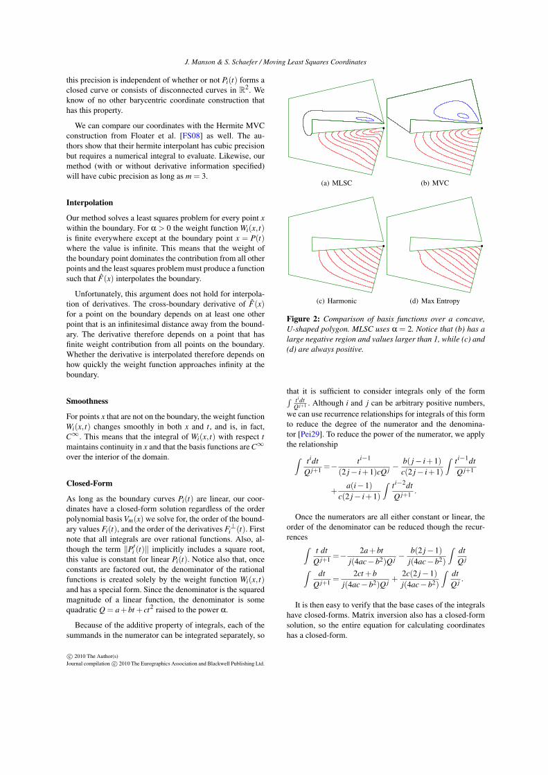
Figure 2: Comparison of basis functions over a concave,U-shaped polygon. MLSC uses α = 2. Notice that (b) has alarge negative region and values larger than 1, while (c) and(d) are always positive.
that it is sufficient to consider integrals only of the form∫ t idtQ j+1 . Although i and j can be arbitrary positive numbers,
we can use recurrence relationships for integrals of this formto reduce the degree of the numerator and the denomina-tor [Pei29]. To reduce the power of the numerator, we applythe relationship∫
t idtQ j+1 =− t i−1
(2 j− i+1)cQ j −b( j− i+1)c(2 j− i+1)
∫t i−1dtQ j+1
+a(i−1)
c(2 j− i+1)
∫t i−2dtQ j+1 .
Once the numerators are all either constant or linear, theorder of the denominator can be reduced though the recur-rences∫
t dtQ j+1 =− 2a+bt
j(4ac−b2)Q j −b(2 j−1)
j(4ac−b2)
∫dtQ j∫
dtQ j+1 =
2ct +bj(4ac−b2)Q j +
2c(2 j−1)j(4ac−b2)
∫dtQ j .
It is then easy to verify that the base cases of the integralshave closed-forms. Matrix inversion also has a closed-formsolution, so the entire equation for calculating coordinateshas a closed-form.
J. Manson & S. Schaefer / Moving Least Squares Coordinates
5. Results
Several types of barycentric coordinates have been describedin the last several years, and we will compare our results withthe most prominent types. For these comparisons, we fit lin-ear polynomials (m = 1) and set α = 2. First, we comparebasis functions in a convex polygon with obtuse angles andshort sides in Figure 1. The vertex associated with the ba-sis function is shown as a black dot. In the image, we showcontour lines for the basis functions at increments of 1
10 . Wedraw the zero contour in black, contours in between 0 and 1in red and negative valued contours in blue.
Among the types of coordinates shown, Harmonic co-ordinates produce the most visually pleasing result, andboth MLSC and MVC have similar looking basis func-tions to Harmonic coordinates. Maximum Entropy coordi-nates exhibit high curvature contours along the short edge.Wachspress coordinates clearly produce undesirable con-tours in this example, because the function value changesvery quickly near the vertex of the basis function. In fact, asthe angle approaches 180 degrees at a vertex, the derivativesof Wachspress coordinates are unbounded.
We also compare methods that are defined over concavepolygons in Figure 2. Polygons that have points in the do-main with small Euclidean distance but large geodesic dis-tance often prove problematic for barycentric coordinates.Again, Harmonic coordinates are typically superior in thissituation because they depend only on geodesic distance andminimize curvature, though at a high computational cost.MEC now compare favorably to MLSC and MVC, becausethey are guaranteed to be positive. This figure also illustratesa tradeoff between MLSC and MVC. MVC produce basisfunctions with lower curvature and more regular shapes, butcan have larger negative regions and larger maximum andminimum values. For example, MVC have values greaterthan 1 in this figure (the contour of value 1 is drawn in yel-low). Negative values are undesirable, because interpolatedvalues may extend beyond the range of the boundary valuesin regions where the basis functions are negative.
In Figure 3 we show an example of the basis functionsthat result from derivative constraints. In this example, func-tion values are linearly interpolated along line segments, butcross boundary derivatives use a quadratic Bezier basis. Thisquadratic basis leaves one degree of freedom for manipulat-ing derivatives, because the values at the ends of the line seg-ments are constrained to match the tangent plane defined bythe function values at the corners. In this figure, the top im-ages show the bases corresponding to a single point withoutderivative constraints (left) and with derivative constraints(right) at increments of 1
10 .
When we add derivative constraints, the basis func-tions corresponding to boundary values must create cross-boundary derivatives with zero magnitude. As a conse-quence, all contour lines are perpendicular to the boundary.We have also observed that Bi, j(x) tend to be positive when
(a) Func Orig. (b) Func Deriv.
(c) Deriv Side 1 (d) Deriv Side 2
Figure 3: Basis functions of our method with derivativesover a concave polygon with α = 2. Above: the basis func-tion of a vertex with and without constrained derivatives.Below: the basis functions of the middle control point of thederivatives.
derivatives are specified. In fact, we have found no examplesin which negative values occur no matter how convolutedthe shape of Pi(t) is. This is in contrast to MVC or evenour own coordinates without derivative constraints, both ofwhich routinely have negative regions in the basis functionswhen applied to non-convex shapes. Unfortunately, we havenot yet found a proof showing that Bi, j(x) is always greaterthan zero in this case.
The bottom images show the basis functions associatedwith the derivative control point at the center of the edgein increments of 1
200 . Note that, in contrast to the basis func-tions associated with the vertices, these derivative basis func-tions can and will be negative, though only very slightly so.In this example, Di,1(x)> −1
100 .
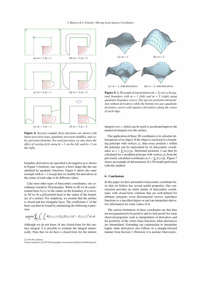
Our construction also defines many members of a familyof coordinates that are all well-defined and have closed-formsolutions. Figure 4 shows six members of this family corre-sponding to different values of α and using different degreepolynomials m in the moving least squares optimization. InFigure 5 (top) we also show interpolation of boundary valueswith m = 1,2 where the boundary data is given by quadraticcurves . Using linear polynomials (m= 1) typically producesbasis functions with the smallest oscillations. While all ofthese coordinates provide linear precision, higher values ofm provide the ability to reproduce functions up to degree massuming that the Fi(t) are also of degree m. When bound-ary derivatives are specified, the utility of fitting higher or-der polynomials becomes clear. If, for example, all of the
J. Manson & S. Schaefer / Moving Least Squares Coordinates
(a) m = 1,α = 1 (b) m = 1,α = 2
(c) m = 2,α = 1 (d) m = 2,α = 2
(e) m = 3,α = 1 (f) m = 3,α = 2
Figure 4: Several example basis functions are shown withlinear precision (top), quadratic precision (middle), and cu-bic precision (bottom). For each precision, we also show theeffect of varying α by using α = 1 on the left, and α = 2 onthe right.
boundary derivatives are specified to be negative as is shownin Figure 5 (bottom), one expects a bowl shape like the oneadmitted by quadratic functions. Figure 6 shows the sameexample with m = 2 except that we modify the derivatives atthe center of each edge to be different values.
Like most other types of barycentric coordinates, our co-ordinates extend to 3D polytopes. While in 2D we fit a poly-nomial basis Vm(x) to the values on the boundary of a curve,in 3D we fit a polynomial basis to the values of the bound-ary of a surface. For simplicity, we assume that the surfaceis closed and has triangular faces. The coefficients C of thebasis can then be found by minimizing the following expres-sion.
argminC
n
∑i=1
∫ 1
0
∫ t
0Wi(x,s, t)(Vm(Pi(s, t))C−Fi(s, t))
2 ds dt
Although we do not know of any closed-form for this sur-face integral, it is possible to evaluate the integral numer-ically. Note that we do have a closed-form for the interior
(a) m = 1 (b) m = 2
(c) m = 1, with derivatives (d) m = 2, with derivatives
Figure 5: A 3D graph of interpolation (α = 2) over a hexag-onal boundary with m = 1 (left) and m = 2 (right) usingquadratic boundary curves. The top row performs interpola-tion without derivatives while the bottom row uses quadraticderivative curves with negative derivatives along the centerof each edge.
integral over s, which can be used to accelerate/improve thenumerical integral over the surface.
One application of these 3D coordinates is to calculate de-formations of an object. If the object is enclosed in a bound-ing polytope with vertices pi, then every position x withinthe polytope can be represented by its barycentric coordi-nates as x = ∑i bi(x)pi. Deformed positions x̂ can then becalculated for a modified polytope with vertices p̂i from thepreviously calculated coordinates as x̂ = ∑i bi(x)p̂i. Figure 7shows an example of deformations of a 3D model performedwith this method.
6. Conclusions
In this paper we have presented a barycentric coordinate ba-sis that we believe has several useful properties. Our con-struction provides an entire family of barycentric coordi-nates with closed-form solutions that are well-defined forarbitrary polygons (even disconnected curves), reproducefunctions to a specified degree m and can interpolate deriva-tive information for some values of α.
The current limitations of these coordinates are that theyare not guaranteed to be positive and we lack proofs for someobserved properties such as interpolation of derivatives andfor positivity of the vertex basis functions when derivativesare interpolated. Extending our construction to interpolatehigher order derivatives also follows in a straight-forwardmanner from Section 3. However, it is unclear what restric-
J. Manson & S. Schaefer / Moving Least Squares Coordinates
(a) positive (b) negative
(c) alternating 1 (d) alternating 2
Figure 6: A hexagon with quadratic function values andderivatives specified along the edges. The derivatives at theend-points are constrained by the function values, but wemodify the derivative in the center of each edge. We con-strain the derivative in the center of the edge to be either allpositive, negative, or alternating in sign.
tions on α must hold in order to guarantee interpolation andwe would like to explore this idea in the future.
References[Bel06] BELYAEV A.: On transfinite barycentric coordinates. In
SGP (2006), pp. 89–99. 2
[DF09] DYKEN C., FLOATER M. S.: Transfinite mean value in-terpolation. CAGD 26, 1 (2009), 117–134. 2
[DMA02] DESBRUN M., MEYER M., ALLIEZ P.: Intrinsic pa-rameterizations of surface meshes. CGF 21, 3 (2002), 209–218.1
[FHK06] FLOATER M., HORMANN K., KÓS G.: A general con-struction of barycentric coordinates over convex polygons. Ad-vances in Computational Mathematics 24, 1 (2006), 311–331. 2
[Flo03] FLOATER M. S.: Mean value coordinates. CAGD 20(2003), 2003. 2
[FS08] FLOATER M. S., SCHULZ C.: Pointwise radial minimiza-tion: Hermite interpolation on arbitrary domains. CGF 27, 5(2008), 1505–1512. 2, 5
[HF06] HORMANN K., FLOATER M. S.: Mean value coordinatesfor arbitrary planar polygons. ACM TOG 25, 4 (2006), 1424–1441. 1, 2
[HS08] HORMANN K., SUKUMAR N.: Maximum entropy coor-dinates for arbitrary polytopes. CGF (Proceedings of SGP) 27, 5(2008), 1513–1520. 2
[JMD∗07] JOSHI P., MEYER M., DEROSE T., GREEN B.,SANOCKI T.: Harmonic coordinates for character articulation.ACM TOG 26, 3 (2007), 71. 2
(a) Rest (b) Pose 1
(c) Pose 2 (d) Pose 3
Figure 7: Example of 3D deformation using our coordi-nates. The rest position is shown on the top left, along withsome example deformations.
[JSW05] JU T., SCHAEFER S., WARREN J.: Mean value coordi-nates for closed triangular meshes. In ACM SIGGRAPH (2005),pp. 561–566. 1
[LD89] LOOP C. T., DEROSE T. D.: A multisided generalizationof bézier surfaces. ACM TOG 8, 3 (1989), 204–234. 1
[LKCOL07] LIPMAN Y., KOPF J., COHEN-OR D., LEVIN D.:Gpu-assisted positive mean value coordinates for mesh deforma-tions. In SGP (2007), pp. 117–124. 2