MOX–Report No. 30/2014 Numerical analysis of Darcy problem on surfaces Ferroni, A.; Formaggia, L.; Fumagalli, A.; MOX, Dipartimento di Matematica “F. Brioschi” Politecnico di Milano, Via Bonardi 9 - 20133 Milano (Italy) [email protected]http://mox.polimi.it
Transcript
MOX–Report No. 30/2014
Numerical analysis of Darcy problem on surfaces
Ferroni, A.; Formaggia, L.; Fumagalli, A.;
MOX, Dipartimento di Matematica “F. Brioschi”Politecnico di Milano, Via Bonardi 9 - 20133 Milano (Italy)
Keywords: PDEs on surfaces, Darcy problem, Mixed finite elements.
AMS Subject Classification:65N30,65N15,76S05
Abstract
Surface problems play a key role in several theoretical and applied fields.In this work the main focus is the presentation of a detailed analysis ofthe approximation of the classical flow porous media problem: the Darcyequation, where the domain is a regular surface. The formulation requirethe mixed form and the numerical approximation consider the classicalpair of finite element spaces: piecewise constant for the scalar fields andRaviart-Thomas for vector fields, both written on the tangential space ofthe surface. The main result is the proof of the order of convergence wherethe discretization error, due to the finite element approximation, is coupledwith a geometrical error. The latter takes into account the approximationof the real surface with a discretized one. Several examples are presented toshow the correctness of the analysis, including surfaces without boundary.
1 Introduction
In several application, like biology [5] or geophysics, the domains where some orpart of problems have to be solved are surfaces or lines. In this particular frame-work several works in literature are present, mainly focused on the derivationand approximation of diffusive processes. Normally the resulting mathemati-cal equations considered involve the classical Laplace-Beltrami operator [9]. Anumerical approximation of this problems is presented in [3, 8, 10, 1] wherestandard Lagrangian finite element spaces are considered.
1
With this choice only the primary unknown field is computed directly, whilea possible secondary unknown, like the tangential gradients, should be com-puted as a post process, often resulting in a poor approximation [4]. In someapplications, e.g. in geophysics, the most important unknowns are often the sec-ondary ones, that represent the fluxes or a macroscopic velocity, which play as atransport for advected quantities. Consequently, we are interested in problemswhere both the primary and secondary unknowns are computed directly. Thisis possible by employing a mixed formulation of the differential problem.An important example of this choice, which is part of the motivations of thepresent paper, are presented in [17, 6, 16, 13, 15]. In this series of papersa reduced model is considered to approximate the flow and pressure fields infractures. The fractures are represented as object of co-dimension one and thereduced models considered are Darcy-type equations written in the tangentialspaces of each fracture. Assuming that the porous matrix is impervious, like in[13], the resulting problem is only written for the fractures.In this work we propose and analyse a mathematical approach to the formulationof Darcy problems on surfaces embedded in R
3. The main part of the paper isdevoted to the derivation of a proper framework for the numerical approximationof such problems. The finite element spaces considered are the classical piecewiseconstant for scalar fields and Raviart-Thomas for vector fields, but projected onthe approximate surface. Particular attention is devoted to the well posednessof the resulting discrete problem and to prove the order of convergence includingalso the geometrical error in the estimation. We allow the surface to be closed sono boundary conditions can be imposed and than suitable additional conditionsshould taking into consideration, such as zero-mean pressure or fixing the valueof the latter in a point of the mesh.The paper is organized as follow. Section 2 introduces the notations used inthe paper as well as the physical problem with some assumptions on the data.The weak formulation of the physical problem and the correct functional settingis described in Section 3, where also the inf-sup condition is proved. Section4 introduces, describes and analyses the numerical approximation where thediscrete inf-sup condition is presented. An error estimation, from the chosendiscretization, is derived in Section 5. In Section 6 a collection of exampleshighlights the potentiality of the proposed methods and the gives a numericalvalidation of the derived theoretical results. Finally, Section 7 is devoted to theconclusions.
2 The governing equations
We assume that the physical domain Γ is a C2 compact, connected orientablemanifold embedded in R
3 described by a signed distance function d : R3 → R
such that
Γ = x ∈ U : d(x) = 0,
2
where U is an open subset of R3 containing Γ. The outward-pointing normal isdefined as n(x) := ∇d(x)/ |∇d(x)|,where ∇d(x) = 0 almost everywhere on Γ.An other quantity that will be useful afterwards is the Hessian matrix H of thedistance function d, where Hij :=
∂2d∂xi∂xj
.
In the sequel, given a function u : Γ → R, we will indicate its lifting, on a givenopen set U containing Γ, as u such that u|Γ = u. The tangential gradient of uwill be then defined as
∇Γu := ∇u− (∇u · n)n. (1)
Introducing P = I − n⊗ n, where ⊗ is the tensor product (a⊗ b)ij = aibj , wecan rewrite (1) as ∇Γu = P∇u. The definition of the tangential divergence isnow straightforward, in fact a smooth given vector field u : Γ → R
3 we have∇Γ · u := P : ∇u.The problem we are interested to solve is the classical Darcy problem [2] definedon the regular surface Γ. The two unknowns are the tangential Darcy velocityu and the pressure p. The problem is defined in the following way
ηu+∇Γp = g in Γ
∇Γ · u = f in Γ
p = p on γD
u · µ = b on γN
, (2)
where µ is the outward unit normal of ∂Γ. The main data in (2) is the inverseof the permeability, defined as
η ∈ L∞ (Γ) and ∃ηmin ∈ R+ : η (x) > ηmin ≥ 0 ∀x ∈ Γ. (3)
We set ηmax = supessx∈Γ η(x). Moreover the scalar source term is defined asf ∈ L2(Γ) and the boundary conditions are imposed on the Darcy velocity u
and on the pressure p. In the former case we consider the function b while forthe latter we have the function p. Finally the vector field g may represent agravity term and the scalar field f may be viewed as a source or a sink. In theforthcoming analysis, to ease the presentation, we will assume that some of theaforementioned data are zero.
3 Weak formulation and functional setting
For simplicity we consider Dirichlet homogeneous boundary conditions, other-wise a lifting technique should be used to impose the boundary data. We intro-duce the weak formulation of problem (2), defining a suitable functional setting.First we introduce the functional space defined on the manifold Γ with its relatednorm
Hdiv(Γ) :=v ∈
[L2(Γ)
]3, ∇Γ · v ∈ L2(Γ)
3
and the norm is
∥v∥2div,Γ := ∥v∥20,Γ + ∥∇Γ · v∥20,Γ,
where ∥·∥0,A is the L2 norm on the regular domain A. In the sequel it will
be useful to introduce the standard scalar product in L2(A), with A a regulardomain, as (·, ·)A. We set the functional space and the norm for the velocity asW , namely
W :=v ∈ Hdiv(Γ), v · n = 0 on Γ,v · µ = 0 on γN
with ∥v∥
W:= ∥v∥div,Γ.
For the pressure field we consider the standard L2 space with its classical norm,we have
Q := L2(Γ) with ∥q∥Q = ∥q∥0,Γ.
If∣∣γD
∣∣ = 0 to recover the uniqueness of the solution, we consider the followingspace for the pressure field
Q := L20(Γ) =
v ∈ L2(Γ) : (v, 1)Γ = 0
with ∥q∥Q = ∥q∥0,Γ,
otherwise the solution is uniquely defined in the quotient space L2(Γ)/R.The weak formulation of the problem (2) is quite standard except the integrationby part of the tangential gradient of the pressure. Taking a test function v ∈ W
and considering the boundary conditions, the pressure gradient term becomes
∫
Γ∇Γp · vdx = −
∫
Γp∇Γ · vdx−
∫
ΓKpv · nHdx+
∫
∂Γpv · µdσ,
where K = ∇Γ ·n. The term which involves the matrix HessianH is zero since wehave required that v·n = 0. We introduce the bilinear forms a(·, ·) : W×W → R
and b(·, ·) : W ×Q → R, defined as
a(u,v) := (ηu,v)Γ , and b(v, q) := − (p,∇Γ · v)Γ
The functionals are F (·) : Q → R and G(·) : W → R, defined as
F (q) := − (f, q)Γ . and G(v) := − (p,v · µ)∂Γ + (g,v)Γ .
The weak formulation of problem (2) is presented in Problem 1.
Problem 1 (Weak formulation) Given η as in (3), find (u, p) ∈ W×Q such
thata(u,v) + b(v, p) = G(v) ∀v ∈ W
b(u, q) = F (q) ∀q ∈ Q. (4)
4
Theorem 3.1 (Well posedness) Under the given hypotheses on the data, Prob-
lem (1) is well posed.
Proof. To ease the presentation we suppose that p and g are zero. However a similarresult can be obtained with different constants. Since (4) is a saddle-point problem wehave to prove the inf-sup condition [4, 12]. By hypothesis we have two positive constantsηmin and ηmax such that ηmin ≤ |η| ≤ ηmax almost everywhere in Γ.We consider the functional space W0 = v ∈ W , b(v, q) = 0 ∀q ∈ Q and we introducev ∈ W0. Then we have ∇Γ · v = 0 almost everywhere in W0 and for each functionin W0 the relation ∥v∥
W= ∥v∥L2(Γ) holds true. Using these results we can prove the
coercivity of a(·, ·)
a(u,u) = (ηu,u)Γ ≥ ηmin∥u∥2L2(Γ) = ηmin∥u∥
2W
∀u ∈ W0.
Then, thanks to the hypothesis on η and the Schwarz inequality we have the continuityof the bilinear form a(·, ·)
|a(u,v)| ≤ ηmax∥u∥W ∥v∥W ∀u,v ∈ W .
Similarly for the bilinear form b(·, ·) we obtain its continuity simply using the Schwarzinequality
|b(v, q)| ≤ ∥∇Γ · v∥L2(Γ)∥q∥L2(Γ) ≤ ∥v∥W
∥q∥Q ∀(v, q) ∈ W ×Q.
Finally we need to prove the inf-sup condition, i.e. there exists a positive constantβ ∈ R
+ such that
∀q ∈ Q, ∃v ∈ W b(v, q) ≥ β∥v∥W ∥q∥Q.
Given a function q ∈ Q we consider the following auxiliary problem
−∇Γ · (∇Γϕ) = q in Γ
ϕ = 0 on γD
∇Γϕ · µ = 0 on γN
. (5)
Problem (5) admits a unique solution ϕ ∈ H2(Γ) such that ∥ϕ∥H2(Γ) ≤ C∥q∥L2(Γ).
Choosing v = ∇Γϕ, from Problem (5) we have −∇Γ · v = q. Considering the aforemen-tioned results, the following inequality holds true
∥v∥2W
= ∥v∥2L2(Γ) + ∥∇Γ · v∥
2L2(Γ) = ∥∇Γϕ∥
2L2(Γ) + ∥q∥
2L2(Γ) ≤
≤ ∥ϕ∥2H2(Γ) + ∥q∥
2L2(Γ) ≤ (C + 1)∥q∥
2L2(Γ).
Imposing C∗ = (C + 1)1
2 we finally obtain the inf-sup condition
b(v, q) = − (q,∇Γ · v)Γ = ∥q∥2L2(Γ) ≥
1
C∗∥v∥
W∥q∥Q,
providing β = 1/C∗. Thanks to this results we can conclude that (1) is well posed.
5
4 Numerical discretization
To provide a discrete formulation for Problem (1) we have to introduce a suitableapproximation of the surface Γ. Following the approach presented in [9], weconsider a polyhedral surface Γh consisting in the union of non overlappingtriangles K, with vertices lying on Γ. We also require the resulting grid to beconforming and regular.Unlike the classical finite elements method, the discrete domain Γh will not ingeneral be included in Γ, thus adding to the approximation error a componentthat accounts for the error introduced by the discretization of the geometry. Toensure a sufficiently good approximation of the surface Γ we assume Γh ⊂ U ,where U is a strip of width δ > 0 in which the decomposition
x = a(x) + d(x)n(x) x ∈ U, (6)
is unique, being a : U → Γ a projection function, d the distance of x from Γand n its normal. Thanks to the regularity of the surface there exists a δ suchthat (6) holds.We set the finite element spaces accordingly with the previous section. We startdefining the space Hdiv(Γh) as
Hdiv(Γh) := vh ∈ [L2(Γh)]3, ∇Γh
· vh ∈ L2(Γh).
Then the finite spaces for velocity and pressure are
where RT0 is the Raviart-Thomas finite elements space of lowest order degree.
If∣∣γD
∣∣ = 0 to recover the uniqueness of the discrete solution, we consider thefollowing discrete space for the pressure field
Qh :=qh ∈ L2(K) : qh|K ∈ P
0(K)∩ L2
0(Γ) with ∥q∥Q = ∥q∥0,Γ,
otherwise the pressure is defined up to a constant.We introduce the bilinear forms for the discrete problem, i.e. ah(·, ·) : Wh ×Wh → R and bh(·, ·) : Wh ×Qh → R, defined as
where fh, ph and gh are an approximation of the data problem on Γh and ∂Γh.We will see in the next section how to choose this approximation. Given theprevious definitions the discrete problem is presented in Problem (2).
6
Problem 2 (Discrete weak formulation) Given η as in (3), find (uh, ph) ∈Wh ×Qh such that
ah(uh,vh) + bh(vh, ph) = Gh(vh) ∀vh ∈ Wh
bh(uh, qh) = Fh(qh) ∀qh ∈ Qh
. (7)
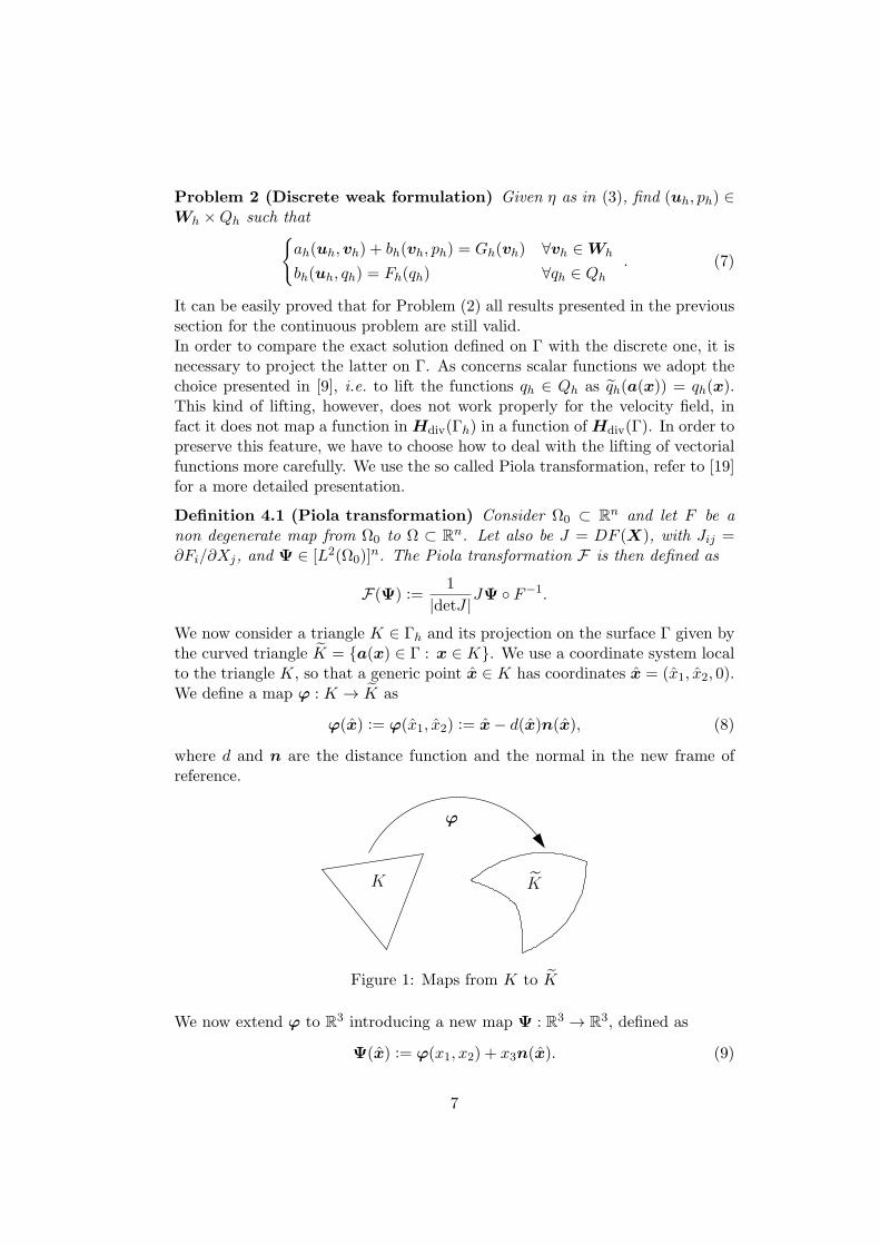
It can be easily proved that for Problem (2) all results presented in the previoussection for the continuous problem are still valid.In order to compare the exact solution defined on Γ with the discrete one, it isnecessary to project the latter on Γ. As concerns scalar functions we adopt thechoice presented in [9], i.e. to lift the functions qh ∈ Qh as qh(a(x)) = qh(x).This kind of lifting, however, does not work properly for the velocity field, infact it does not map a function in Hdiv(Γh) in a function of Hdiv(Γ). In order topreserve this feature, we have to choose how to deal with the lifting of vectorialfunctions more carefully. We use the so called Piola transformation, refer to [19]for a more detailed presentation.
Definition 4.1 (Piola transformation) Consider Ω0 ⊂ Rn and let F be a
non degenerate map from Ω0 to Ω ⊂ Rn. Let also be J = DF (X), with Jij =
∂Fi/∂Xj, and Ψ ∈ [L2(Ω0)]n. The Piola transformation F is then defined as
F(Ψ) :=1
|detJ |JΨ F−1.
We now consider a triangle K ∈ Γh and its projection on the surface Γ given bythe curved triangle K = a(x) ∈ Γ : x ∈ K. We use a coordinate system localto the triangle K, so that a generic point x ∈ K has coordinates x = (x1, x2, 0).We define a map ϕ : K → K as
ϕ(x) := ϕ(x1, x2) := x− d(x)n(x), (8)
where d and n are the distance function and the normal in the new frame ofreference.
K K
ϕ
Figure 1: Maps from K to K
We now extend ϕ to R3 introducing a new map Ψ : R3 → R
3, defined as
Ψ(x) := ϕ(x1, x2) + x3n(x). (9)
7
The map Ψ is the one we consider for the construction of the Piola transforma-tion.The lifting of a scalar function qh : K → R to qh : K → R is therefore given by
qh(Ψ(x)) = qh(x) x ∈ K. (10)
Given F := ∇Ψ, the lifting of a vectorial function wh : K → R3 to wh : K → R
3
is defined as
wh(Ψ(x)) =1
|detF |Fwh(x) x ∈ K. (11)
The matrix F has the following structure
F = [t1 t2 n] , (12)
where ti = ∂ϕ/∂xi, i = 1, 2 has components ti,j = δji−njni−dHji for j = 1, 2, 3with H the Hessian of the distance function d.
Remark 1 It is immediate to show that ti · n = 0 for i = 1, 2.
Since dσ = |t1 ∧ t2|dσh and detF = (t1 ∧ t2) · n we have dσ = ξhdσh whereξh = |detF |.
Remark 2 The matrix F is defined element wise. If we glue together all the
local F , we find a global matrix that, to ease the notation, we will still indicate
as F . In the following it will be clear from the domain of integration if we are
referring to the local map or to the global one.
We recall a useful lemma about the properties of the considered geometry. Fora complete proof refer to [10].
Lemma 4.1 Assume Γ and Γh defined as above. Then
∥d∥L∞(Γh) ≤ ch2.
Moreover, the quotient ξh = dσ/dσh previously defined satisfies
∥1− ξh∥L∞(Γh) ≤ ch2.
We now deduce an important relationship between functions defined on K andtheir lifting on K. We consider a couple of functions (wh, qh) ∈ Wh × Qh and
the corresponding lifting (wh, qh) ∈ Wh × Qh, where Wh and Qh are defined as
The last equality holds for all qh ∈ Qh and so we can conclude that
∇Γ · wh =1
ξh∇Γh
·wh a.e. in K. (13)
Now we are able to prove the following
Lemma 4.2 Given (wh, qh) ∈ Wh × Qh and the corresponding lifting onto Γ
(wh, qh) ∈ Wh × Qh, then exists some constants such that the following inequal-
ities hold
1
C1∥qh∥L2(K) ≤ ∥qh∥L2(K)
≤ C1∥qh∥L2(K)
1
C2∥wh∥L2(K) ≤ ∥wh∥L2(K)
≤ C2∥wh∥L2(K)
1
C3∥∇Γh
·wh∥L2(K) ≤ ∥∇Γ · wh∥L2(K)≤ C3∥∇Γh
·wh∥L2(K)
Proof. The first inequality is proved in [9]. For the second inequality we have by thedefinition of the L2-norm
∥wh∥2L2(K) = (wh, wh)K =
(1
ξhF⊤Fwh,wh
)
K
.
9
Matrix F⊤F is given by
F⊤F =
|t1|
2t1 · t2 0
t1 · t2 |t2|2
00 0 1
.
From the definition of t1 and t2 it is straightforward that
|ti|2= 1 +O(h2) and t1 · t2 ≈ −n1n2 +O(h2).
Following [10] we have that exists c ∈ R+ such that ∥ni∥L∞(K) ≤ ch, i = 1, 2, 3, then
∥t1 · t2∥L∞(K) ≤ ch2.
In conclusion the following inequality holds
∥∥I − F⊤F∥∥L∞(K)
≤ ch2.
Thanks to this last relation and to lemma (4.1) the second estimate immediately follows.In order to prove the last inequality, using (13), we can write
∥∇Γ · wh∥2L2(K) = (∇Γ · wh,∇Γ · wh)K =
(1
ξh∇Γh
·wh,∇Γ · wh
)
K
.
Using this relation and the estimate for ξh we can obtain the last inequality.
5 Error analysis
In this section, to ease the analysis and the presentation of the forthcomingresults, we consider fully homogeneous boundary conditions and zero vectorsource term. Thanks to the results of the previous section we can obtain thefollowing useful relation
∫
K
∇Γ · wh qh dσ =
∫
K
∇Γh·wh qh dσh. (14)
Therefore the approximation of the bilinear form b(·, ·) with bh(·, ·) will not bringany additional error due to the discretization of the geometry. The additionalterm is only linked to the approximation of the bilinear form a(·, ·), in particularfrom
∫
K
ηuh · vh dσh =
∫
K
ηξh
(F−⊤F−1uh
)· vh dσ. (15)
If we define Bh := ξhF−⊤F−1 we can rewrite the discrete Problem 2 as
(ηBhuh, vh)Γ − (ph,∇Γ · vh)Γ = 0 ∀vh ∈ Wh,
(qh,∇Γ · uh)Γ = (f, qh)Γ ∀qh ∈ Qh.(16)
In this case we have chosen fh(x) = ξhf(Ψ(x)) in order to have Fh = F on Γ.
10
Remark 3 In practice is often simpler to compute the source term as fh(x) =f(Ψ(x)), thus adding an extra term of order O(h2) to the error given by the
difference between f and Fh.
Lemma 5.1 If (uh, ph) is solution of (7), then its correspondent lift to Γ, in-dicated with (uh, ph), is solution of (16) and vice versa.
Proof. Thanks to relations (14) and (15) we immediately get the equivalence between
problems (7) and (16).
To provide an error estimate for our problem we need to recall some resultson saddle-points problems, see [4, 18] for a detailed analyses. Introducing the
following discrete functional space Wfh := wh ∈ Wh : (qh,∇Γ · wh − f)Γ =
0 ∀qh ∈ Qh, the Lemma 5.2 holds true [18].
Lemma 5.2 If the spaces Wh and Qh satisfy the inf-sup condition then for each
f ∈ L2(Γ) there exist a unique wfh ∈ (W 0
h )⊥ such that:
(qh,∇Γ · wfh − f)Γ = 0 ∀qh ∈ Qh (17)
and∥∥∥wf
h
∥∥∥W
≤1
βsup
qh∈Qh,qh =0
(f, qh)Γ∥qh∥Q
. (18)
Furthermore if uh ∈ Wh satisfies
(ηBhuh, vh)Γ = 0 ∀vh ∈ W 0h ,
then there exists a unique ph ∈ Qh such that
− (ph,∇Γ · vh)Γ + (ηBhuh, vh)Γ = 0 ∀vh ∈ Wh (19)
and
∥ph∥L2 ≤1
βsup
vh∈Wh,vh =0
(ηBhuh, vh)Γ∥vh∥W
. (20)
By setting uh = u0h + w
fh, with u0
h ∈ W 0h and w
fh ∈ W
fh , we can rewrite (16) as
: find u0h ∈ W 0h such that:
(ηBhu
0h, vh
)Γ= −
(ηBhw
fh, vh
)Γ
∀vh ∈ W 0h . (21)
Thanks to the Lax-Milgram Theorem, it exists a unique solution u0h ∈ W 0
h of
(21) which satisfies ∥u0h∥W ≤ C∥wf
h∥L2 , for a C > 0. Then, from (18) and (20)we have:
∥uh∥W ≤C
β∥f∥L2 and ∥ph∥L2 ≤
C
β∥uh∥L2 .
11
To find an estimate for the discretization error we write (16) in the followingform, which highlights the classical saddle point structure:
By subtracting (1) and (22) and adding and subtracting to the result a vector
w∗h ∈ W
fh , we obtain
(η(uh − w∗h), vh)Γ + (p− ph,∇Γ · vh)Γ = (η(u− w∗
h), vh)Γ + (η(I −Bh)uh, vh)Γ
By choosing vh = uh − w∗h, with vh ∈ Wh, and using (5), we get:
∥vh∥W ≤ C (∥u− w∗h∥L2 + ∥I −BH∥L∞∥f∥L2) ,
from which it follows that
∥u− uh∥W ≤ C
(inf
w∗
h∈W
fh
∥u− w∗h∥W + ∥I −BH∥L∞∥f∥L2
).
Now we want to show that
infw∗
h∈W
fh
∥u− w∗h∥W ≤ C inf
vh∈Wh
∥u− vh∥W . (23)
From Lemma 5.2, for all vh ∈ Wh, there exists a unique zh ∈ (W 0h )
⊥ such that
(qh,∇Γ · zh)Γ = (qh,∇Γ · (u− vh))Γ ∀qh ∈ Qh,
and ∥zh∥W ≤ C∥∇Γ · (u − vh)∥L2 . Setting w∗h = zh + vh, we have w∗
h ∈ Wfh
and we obtain ∥u− w∗h∥W ≤ ∥u− vh∥W , from which (23) follows.
Repeating a similar analysis for the pressure, we get the final inequality
∥u− uh∥W + ∥p− ph∥Q ≤ C
(∥I −Bh∥L∞∥f∥L2 +
+ infvh∈Wh
∥u− vh∥W + infqh∈Qh
∥p− qh∥Q
).
(24)
In (24) we observe that, as we expected, the error is composed by two differentterms, the first related to the finite element discretization and the second relatedto the approximation of the geometry of the problem. In particular, as seen inthe previous section for F⊤F , we can immediately conclude that
∥I −Bh∥L∞(Γ) ≤ ch2.
Thus the contribution of the geometric error in a Darcy problem is of the secondorder respect to grid size h.We prove the main result of this section.
12
Theorem 5.1 (Order of convergence) Let (u, p) ∈ W × Q be the solution
of the continuous problem (4), (uh, ph) ∈ Wh × Qh the solution of the discrete
problem (7) and (uh, ph) ∈ Wh × Qh its corresponding lift to Γ. Assuming that
the solution is regular enough and that ξh ∈ H1(K), then the following inequality
Proof. If we neglect in (24) the geometric contribution to the error, we have
∥u− uh∥W + ∥p− ph∥Q ≤
(inf
wh∈Wh
∥u− wh∥W + infqh∈Qh
∥p− qh∥Q
)
We start considering the estimate for the velocity field and we introduce the functionu : Γh → R
3, defined as follows
u(x) := ξh F−1u(Ψ(x)) with x ∈ Γh.
So u is the projection of the exact solution on discrete surface. Thanks to lemma (4.2)we have
∥u− wh∥Hdiv(K) ≤ ∥u−wh∥Hdiv(K),
This relation, together with standard results for Hdiv, gives us
∥u− wh∥Hdiv(K) ≤ Chk
(|∇Γh
· u|H1(K) + |u|Hdiv(K)
).
We see now how to estimate the right hand side of the inequality. From the definitionof the H1 semi-norm it follows that
|∇Γh· u|
2H1(K) = ∥∇Γh
(∇Γh· u)∥
2L2(K) = (∇Γh
(∇Γh· u),∇Γh
(∇Γh· u))K .
From [11] and (13) we obtain ∇Γh(∇Γh
· u) = Ph(I − dH)∇Γ(ξh∇Γ · u), that insertedin the semi-norm definition gives us
|∇Γh· u|
2H1(K) = (Ah∇Γ(ξh∇Γ · u),∇Γ(ξh∇Γ · u))K ,
where Ah is defined as Ah := P (I−dH)Ph(I−dH)P/ξh. We know that ξ−1h is bounded
and moreover, from [9], we have
P (I − dH)Ph(I − dH)P ≈ PPhP +O(h2).
That becomes
PPhP = P − (nh − (nh · n)n)(nh − (nh · n)n)⊤.
Because in the reference system local to the triangle K, we have nh = e3, then
|nh − (nh · n)n| = |e3 − n3n| =√
1− n23 =
√n21 + n2
2 ≈ O(h).
13
Therefore for matrix Ah holds the relation Ah ≈ P + O(h2), Moreover, thanks to theregularity of the surface P is bounded and so it is Ah. Then we can obtain
|∇Γh· u|H1(K) ≤ ∥Ah∥
1
2
L∞(K)∥∇Γ(ξh ∇Γ · u)∥
L2(K)
Applying triangular and Schwarz’s inequalities
∥∇Γ(ξh ∇Γ · u)∥L2(K) ≤ ∥∇Γξh∥L2(K)∥∇Γ · u∥
L2(K)+
+∥ξh∥L2(K)∥∇Γ(∇Γ · u)∥L2(K) ≤ C∗∥∇Γ · u∥
H1(K),
where C∗ = max∥∇Γξh ∥L2(K), ∥ξh∥L2(K)
. Defining C1 = C∗∥Ah∥
1
2
L∞(K), we have
proved that
|∇Γh· u|H1(K) ≤ C1∥∇Γ · u∥
H1(K). (25)
In analogous way we can show the following inequality for the semi-norm
|u|H1(K) ≤ C2∥u∥H1(K). (26)
Summing (25) and (26) over all triangles we obtain the velocity estimate. We considernow the estimate for pressure and, similarly to what we have done for velocity, weintroduce the lift of the exact solution p to Γh as
p(x) := p(Ψ(x)) with x ∈ Γh.
From lemma (4.2) and from standard interpolation results we have
∥p− qh∥L2(K) ≤ C∥p− qh∥L2(K) ≤ C3hK |p|H1(K) .
Finally we exploit the results of [9] and we obtain
∥p− qh∥L2(K) ≤ CC3hK |p|H1(K) .
Considering the contribution of all the elements we have the desired estimation for the
pressure.
6 Applicative examples
We present in the following sub-sections some examples to show the goodnessof the proposed approximation. In particular we show the error convergence fortwo different geometries: a sphere and a toroid. The choice is driven by theanalytical solutions proposed in the literature for these geometries. The resultsare in good agreement with the theory. The simulations we propose in thispaper are performed using the library for finite elements LifeV [14] developedby Ecole Polytechnique Federale de Lausanne (CMCS), Politecnico di Milano(MOX), INRIA under the projects REO and ESTIME and Emory University(Math&CS). Finally to ensure that the geometrical error is small enough and toincrease the accurateness of the numerical solution, we have used the softwarepresented in [7] to increase the grids quality.
14
6.1 Order of convergence
We consider problem (2) solved on two different domains Γ1 and Γ2, wherethe former is a unit sphere while the latter a spherical cup limited by θ ∈[−π/2, π/2] and φ ∈ [0, 2π]. A unit permeability is considered and the scalarsource term is taken as f(θ, φ) = 2(2 cos2 θ− sin2 θ) such that the exact solutionis p(θ, φ) = cos2 θ. For Γ1 the problem does not require boundary condition,hence to have a well-posed problem we impose the solution in one point. Whilefor Γ2 we consider Dirichlet boundary conditions equal to the exact solution.The advantage of using a spherical domain, in addition to the use of sphericalcoordinate in finding the exact solution, is that we explicitly know the distancefunction d(x) = |x| − 1.
0.001
0.01
0.1
1
0.01 0.1
error
h
Spherical cup
Sphere
reference O (h)
Figure 2: Error decay for the sphere and the spherical cup compared with areference curve of O (h).
In Figure 2 we present the error history, for the two problems, decreasing themesh thickness. It is clear that in both cases the error obtained scales at least asO (h), confirming the theoretical result presented in Theorem 5.1. Observingthe solutions reported in Figure 3, for the sphere, and in Figure 4, for thespherical cup, we can notice that the velocity field obtained is tangent to thesurface and flows in the opposite direction of the pressure gradient, as we expectfrom the Darcy’s law.
6.2 Example 2
In this second example we consider as surface a torus defined by
Γ =
(x, y, z) ∈ R
3 :(√
x2 + y2 − 1)2
+ z2 − 0.62 = 0
.
15
y
z
x
p
0
0.25
0.5
0.75
1
Figure 3: Numerical solution on the unit sphere. Both pressure and velocityare represented. The arrows for the latter are coloured and sized as the velocitymagnitude. We can notice that the in the two poles of the sphere and in itsequator the pressure change slowly so does the velocity.
y
z
x
(a) Solution for a fine mesh (b) Solution for a coarse mesh
p
0.5
0.6
0.8
1
Figure 4: Numerical solution on a spherical cup of a unit sphere. Both pressureand velocity are represented. The arrows for the latter are coloured and sizedas the velocity magnitude. We can see that the solution is more smooth refiningthe mesh.
16
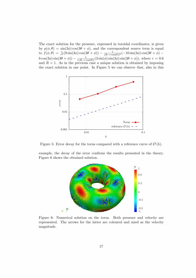
The exact solution for the pressure, expressed in toroidal coordinates, is givenby p(φ, θ) = sin(3φ) cos(3θ + φ), and the correspondent source term is equalto f(φ, θ) = 1
r2(9 sin(3φ) cos(3θ + φ)) − 1
(R−r cos(θ))2(−10 sin(3φ) cos(3θ + φ) −
6 cos(3φ) sin(3θ + φ)) − 1r(R−r cos(θ))(3 sin(φ) sin(3φ) sin(3θ + φ)), where r = 0.6
and R = 1. As in the previous case a unique solution is obtained by imposingthe exact solution in one point. In Figure 5 we can observe that, also in this
0.001
0.01
0.1
1
0.01 0.1
error
h
Torus
reference O (h)
Figure 5: Error decay for the torus compared with a reference curve of O (h).
example, the decay of the error confirms the results presented in the theory.Figure 6 shows the obtained solution.
y
z x
p1
0.8
0.4
-0.4
-0.8-1
0
Figure 6: Numerical solution on the torus. Both pressure and velocity arerepresented. The arrows for the latter are coloured and sized as the velocitymagnitude.
17
7 Conclusions
In this work we have presented a framework to solve Darcy problems on regularmanifolds. The numerical discretization chosen is the classical pair of piece-wise constant, for the pressure, and lowest order tangential Raviart-Thomas,for the Darcy velocity, finite element spaces. In this context we have providedan analysis of the relations between the quantities defined on the real surfaceand the ones defined on its discretization. Then we have used this properties inorder to prove some results for the convergence of the approximation error. Thenumerical experiments proposed have confirmed the estimate presented in thetheory.A possible development, following the reduced model proposed in [17, 6, 16, 13,15], of the work could be the application of the results obtained in more realisticcases, for example in solving the Darcy problem defined in a whole basin. Insuch a case we should introduce suitable coupling conditions between the domainand the reduced model of the fracture and, in the case of a network of fractures,we should provide models for the flow along the intersecting curves.
8 Acknowledgements
The authors wish to thank Antonio Cervone, Franco Dassi, Guido Iori and AnnaScotti for many fruitful discussions.
References
[1] Paola F. Antonietti, Andreas Dedner, Pravin Madhavan, Simone Stan-galino, Bjorn Stinner, and Marco Verani. High order discontinuous galerkinmethods on surfaces. Technical report, Politecnico di Milano, 2014.
[2] Jacob Bear. Dynamics of Fluids in Porous Media. American Elsevier, 1972.
[3] Marcelo Bertalmıo, Li-Tien Cheng, Stanley Osher, and Guillermo Sapiro.Variational problems and partial differential equations on implicit surfaces.Journal of Computational Physics, 174(2):759–780, 2001.
[4] Franco Brezzi and Michel Fortin. Mixed and Hybrid Finite Element Meth-
ods, volume 15 of Computational Mathematics. Springer Verlag, Berlin,1991.
[5] Chris D. Cantwell, Sergey Yakovlev, Robert M. Kirby, Nicholas S. Peters,and Spencer J. Sherwin. High-order spectral/hp element discretisation forreaction-diffusion problems on surfaces: Application to cardiac electrophys-iology. J. Comput. Phys., 257:813–829, January 2014.
18
[6] Carlo D’Angelo and Anna Scotti. A mixed finite element method for Darcyflow in fractured porous media with non-matching grids. Mathematical
Modelling and Numerical Analysis, 46(02):465–489, 2012.
[7] Franco Dassi, Simona Perotto, Luca Formaggia, and Paolo Ruffo. Efficientgeometric reconstruction of complex geological structures. Mathematics and
Computers in Simulation, 2014.
[8] Alan Demlow and Gerhard Dziuk. An adaptive finite element method forthe Laplace-Beltrami operator on implicitly defined surfaces. SIAM Journal
on Numerical Analysis, 45(1):421–442, 2007.
[9] Gerhard Dziuk. Finite elements for the beltrami operator on arbitrarysurfaces. In Stefan Hildebrandt and Rolf Leis, editors, Partial Differential
Equations and Calculus of Variations, volume 1357 of Lecture Notes in
Mathematics, pages 142–155. Springer Berlin Heidelberg, 1988.
[10] Gerhard Dziuk and Charles M Elliott. Finite elements on evolving surfaces.IMA journal of numerical analysis, 27(2):262–292, 2007.
[11] Gerhard Dziuk and Charles M Elliott. Surface finite elements for parabolicequations. Journal of Computational Mathematics, 25(4), 2007.
[12] Alexandre Ern and Jean-Luc Guermond. Theory and practice of finite ele-
[13] Luca Formaggia, Alessio Fumagalli, Anna Scotti, and Paolo Ruffo. A re-duced model for Darcy’s problem in networks of fractures. ESAIM: Math-
ematical Modelling and Numerical Analysis, 48:1089–1116, 7 2014.
[14] Gilles Fourestey and Simone Deparis. Lifev user manual. http://lifev.
org, November 2010.
[15] Alessio Fumagalli and Anna Scotti. A numerical method for two-phase flowin fractured porous media with non-matching grids. Advances in Water Re-
sources, 62, Part C(0):454–464, 2013. Computational Methods in GeologicCO2 Sequestration.
[16] Alessio Fumagalli and Anna Scotti. An efficient xfem approximation ofdarcy flow in arbitrarly fractured porous media. Oil and Gas Sciences and
Technologies - Revue d’IFP Energies Nouvelles, April 2014.
[17] Vincent Martin, Jerome Jaffre, and Jean E. Roberts. Modeling fracturesand barriers as interfaces for flow in porous media. SIAM J. Sci. Comput.,26(5):1667–1691, 2005.
[18] Alfio Quarteroni and Alberto Valli. Numerical approximation of partial dif-
ferential equations, volume 23 of Springer Series in Computational Mathe-
matics. Springer-Verlag, Berlin, 1994.
19
[19] Marie E Rognes, Robert C Kirby, and Anders Logg. Efficient assembly ofh(div) and h(curl) conforming finite elements. SIAM Journal on Scientific
Computing, 31(6):4130–4151, 2009.
20
MOX Technical Reports, last issuesDipartimento di Matematica “F. Brioschi”,
Politecnico di Milano, Via Bonardi 9 - 20133 Milano (Italy)
Optimal techniques to simulate flow in fractured reservoirs
27/2014 Vergara, C; Domanin, M; Guerciotti, B; Lancellotti, R.M.;
Azzimonti, L; Forzenigo, L; Pozzoli, M
Computational comparison of fluid-dynamics in carotids before and af-ter endarterectomy
26/2014 Discacciati, M.; Gervasio, P.; Quarteroni, A.
Interface Control Domain Decomposition (ICDD) Methods for Hetero-geneous Problems
25/2014 Hron, K.; Menafoglio, A.; Templ, M.; Hruzova K.; Filz-
moser, P.
Simplicial principal component analysis for density functions in Bayesspaces
24/2014 Ieva, F., Jackson, C.H., Sharples, L.D.
Multi-State modelling of repeated hospitalisation and death in patientswith Heart Failure: the use of large administrative databases in clinicalepidemiology
23/2014 Ieva, F., Paganoni, A.M., Tarabelloni, N.
Covariance Based Unsupervised Classification in Functional Data Anal-ysis
22/2014 Arioli, G.
Insegnare Matematica con Mathematica
21/2014 Artina, M.; Fornasier, M.; Micheletti, S.; Perotto, S.
The benefits of anisotropic mesh adaptation for brittle fractures underplane-strain conditions