MS #2007-0051-2 Inter-city Compensating Wage Differentials and Intra-city Workplace Centralization (Old title: An Inter-urban Wage Test of the Monocentric Model) Jim Dewey Bureau of Economic and Business Research University of Florida Gabriel Montes Rojas 1 Bureau of Economic and Business Research University of Florida and City University London Working Paper Submitted to Regional Science and Urban Economics This version: March 2008 1 Corresponding Author: e-mail: [email protected]. Address: 221 Matherly Hall, Post Office Box 117145, Gainesville, Florida 32611-7145, tel.: (352)-392-0171 (ext.214), fax: (352)-392-4739. We are grateful to Richard Arnott and three anonymous referees for their very valuable comments and suggestions.
Transcript
MS #2007-0051-2 Inter-city Compensating Wage Differentials and Intra-city Workplace Centralization
(Old title: An Inter-urban Wage Test of the Monocentric Model)
Jim Dewey Bureau of Economic and Business Research
University of Florida
Gabriel Montes Rojas1 Bureau of Economic and Business Research
University of Florida and
City University London
Working Paper Submitted to
Regional Science and Urban Economics This version: March 2008
1 Corresponding Author: e-mail: [email protected]. Address: 221 Matherly Hall, Post Office Box 117145, Gainesville, Florida 32611-7145, tel.: (352)-392-0171 (ext.214), fax: (352)-392-4739. We are grateful to Richard Arnott and three anonymous referees for their very valuable comments and suggestions.
2
Abstract: We explore the interaction of inter-city and intra-city compensating wage
differentials by occupation. Our conjecture is that more central occupations receive
higher wage premiums in larger cities, since workers in those occupations face a less
desirable locus of housing prices and commuting times than those who have jobs in
residential areas. The two main contributions of the paper are: 1) construction of an index
of occupational centralization that accounts for differences between the density of
employment where job holders in an occupation work and the overall employment
density pattern, and 2) empirical confirmation that compensating differentials in larger
cities are larger for more central occupations. The results are robust to the inclusion of
individual-specific human capital variables and city-specific controls. These findings
have implications for wage indexes used to construct real wage measures for academic
research or in funding formulas where resource allocations are adjusted for labor cost
The theory of spatial compensating differentials developed largely along two paths.
Studies focused on intra-city rent and wage gradients followed the Alonso-Muth-Mills
model (Alonso, 1962, Muth, 1969 and Mills, 1972). Studies focused on inter-city
variation in wages and rents followed the Rosen-Roback model (Rosen 1972 and Roback
1982 and 1988). The Rosen-Roback framework continues to have numerous practical
applications in research and policy. Gabriel and Rosenthal (2004) is one recent example
of numerous studies measuring urban quality of life and the quality of the business
environment. Moretti (2004) applies this model to measure human capital spillovers.
Glaeser (1998) analyzes proposals to adjust transfer payments for differences in local cost
3
of living. To equalize educational opportunity across school districts, many states adjust
funding for differences in the cost of hiring similarly qualified teachers in different cities
(National Conference of State Legislatures, 2008). Implicitly or explicitly, these policies
are based on the measurement of inter-city compensating wage differentials (Fowler and
Monk, 2001).
Typically, studies of inter-city compensating differentials ignore intra-city
centralization and the resulting intra-city rent and wage gradients. However, if rents are
differentially higher in the denser areas of larger cities, inter-city compensating
differentials in larger cities must be larger for more centralized jobs than for less
centralized jobs in equilibrium. Thus, we argue that correct inter-city wage comparisons
must hold constant the relative location of employment within cities. We have two main
objectives; first, to develop a measure of job centrality that may be practically applied to
the estimation of inter-city compensating wage differentials across a wide range of cities,
and second, to test the hypothesis that more centralized employment locations lead to
larger compensating differentials in larger cities.
Data on wages, individual characteristics, job characteristics, and within city
workplace location is available for only a small number of cities. Our empirical strategy
is to construct an index of occupational centralization for 475 occupational classifications
for seven US cities where such data is available with sufficient geographic detail. We
find that occupational centralization is quite consistent across these cities. We then use
this index to proxy within city workplace location in a regression of individual level
wages across 272 US Metropolitan Statistical Areas (we use the terms MSA and city
interchangeably). Interacting the occupational centrality index with the log of total MSA
employment, we find very strong evidence that occupations that tend to locate more
4
centrally receive larger wage premiums in larger MSAs than do occupations that tend to
locate less centrally.
Three related phenomena may interfere with identification of the impact of
centralization on inter-city compensating differentials. First is the possibility that workers
in more central occupations are more educated and the return to education is higher in
larger cities. Second is the possibility that more skilled members of central occupations
are more likely to sort into larger cites in response to higher returns to skill. Third is the
possibility that more educated workers (who tend be in more central occupations) have
stronger preferences for the increased urban amenities in larger cities and more central
locations (Glaeser, Kolko and Saiz, 2001). We argue that our inclusion of detailed
individual characteristics, MSA and occupation dummy variables, and, especially, an
interaction between education and the log of total MSA employment controls as far as
possible for these confounding influences.2
The remainder of the paper is organized as follows. Section 2 presents some
stylized facts related to our main hypothesis. Section 3 considers the theoretical
background and underpinnings of our argument. Section 4 details our measure of
occupational centrality and describes other data used in our analysis. Section 5 presents
the econometric analysis. Section 6 considers the implications of our findings for the
construction of wage indices. Section 7 concludes.
2. Some stylized facts and main hypothesis
If an occupation is central, then its workers face a less favorable trade-off between
commuting time and high rents, and as a result wage premiums should increase more
2 We are indebted to Richard Arnott for pointing out the potential effect of higher preferences for urban amenities among the educated and for suggesting the interaction between education and city size as a control for these sorting issues.
5
with city size relative to non-central occupations. As an example, consider lawyers who
rank at the top of occupations in terms of centrality (see Table 3 below) and production
workers, who are in the least central occupation categories. Also consider the relative
city-occupation wage premium constructed asPc
Lc
ww
,
, , where jcw , denotes the average wage
in city c and occupation j (=L: lawyers, P: production workers) (see the following
section for details about how these variables were constructed).
Figure 1 reports the relative wage premiums for these two occupations as a
function of city size, where this is measured by the logarithm of total employment. The
figure shows that the relative premium increases with city size. We attribute this to
differences in the occupation centrality, that is, to the fact that lawyers are more likely to
work in the Central Business District (CBD), and therefore require a higher relative
compensation in large cities than production workers. The empirical analysis below
shows that this result can be extended to all occupations, and that it is robust to the
inclusion of additional controls.
In order to understand the usefulness of this result, consider the example of a
generic firm that is considering moving to a city which exactly doubles the employment
size. Moreover, assume that this firm has two types of workers, legal and production
workers, and that it seeks for the right compensation scheme to keep its employees
exactly indifferent between working in the small and the big city. In both cities, lawyers
would be working in its downtown office and production workers in its outskirts
assembly plant. The firm needs to adjust wages in order to compensate its workers for the
higher cost of living or higher commuting time, but should the firm adjust wages equally
for all occupations? The results in Section 5 imply that legal workers, a typical central
6
occupation, should receive a higher premium than production workers. In other words,
intra-firm wage differences will increase as a result of moving to a larger city.
Is this the result of a more general pattern? In order to answer this question we run
a simple regression model for each occupation category, where the log of the average
wage in each MSA is regressed against our measure of city size, log of total
employment3. In each case we obtain 475 regression coefficients (one for each
occupation) that measure how wages in each occupation are related to city size. If our
hypothesis is true, more central occupation should have larger coefficients than non-
central occupations. Then, we plot them against the centrality index constructed as in the
following section. The positive relation depicted in Figure 2 confirms the hypothesis that
more central occupations receive higher premiums in larger cities (with logarithm of
employment t-stat=5.84, R2=0.07).
3. Background and Theoretical Underpinnings
The framework developed by Rosen (1979) and Roback (1982, 1988) explains rent and
wage variation across cities in terms of intrinsic city characteristics, defined broadly as
amenities (consumptive or productive). In these models workers require higher salaries
when faced with higher housing prices or rent at a given consumptive amenity level.
Similarly, at a given productivity level, firms would offer lower wages when faced with
higher rents. Assuming the supply of land for household and firm use is not perfectly
elastic, rent grows with city size, and wages, rent, and city size adjust to maintain
compensating differentials for differences in intrinsic characteristics in equilibrium.
3 Similar results are obtained when total employment is replaced by average commuting time as a proxy for city size.
7
Productive amenities, such as infrastructure quality, increase the number of firms
wishing to locate in the city at a given rent and wage level. The resulting upward pressure
on rent means wages must be higher to compensate workers. Consumptive amenities,
such as good weather, increase the number of workers that wish to locate in a city at any
given rent and wage level. The resulting upward pressure on rents means wages must be
lower to compensate firms. In the presence of agglomeration economies, an increase in
city size due to either productive or consumptive amenities makes the city more attractive
to firms. This additional upward pressure on rents exacerbates the increase in wages due
to city specific productive amenities and mitigates or may overwhelm wage reductions
due to consumptive amenities.
The traditional intra-urban wage theory was built around the Alonso-Muth-Mills
monocentric model where residents choose their proximity to the CBD where all
production takes place, trading higher rents against shorter commuting times (Alonso,
1962, Muth, 1969 and Mills, 1972; Brueckner, 1987, Straszheim, 1987 and White, 1999
provide excellent reviews). Extensions of the basic model incorporated local
employment, endogenous center formation with agglomeration economies, and
polycentric employment cities in which several employment centers arise simultaneously
(for example Solow 1973, White 1988 and 1999, Fujita and Ogawa 1982, and Anas and
Kim 1996). Anas, Arnott and Small (1998) provide a general discussion of the modern
urban structure.
Centralization in such models may arise from intrinsic advantages at particular
locations, such as transportation nodes, or, perhaps more fundamentally, from
agglomeration economies owing to increasing returns to scale or to the potential for
increased creative interaction. Whatever the reason for centralization, rent increases with
8
distance from the urban fringe and with density for any given city size. Further, density
and rent at any particular location increase with city size. Rent at the urban fringe is
determined by the opportunity cost of land in non urban uses. Wages are in turn higher at
employment locations with higher rents to compensate workers for a less desirable locus
of housing prices and commuting times. Eberts (1981), Ihlanfeldt (1992) and McMillen
and Singer (1992) find surprisingly strong empirical support for the hypothesis that
wages for otherwise similar jobs rise as employment location becomes more centralized.
We argue that centralization and the resulting intra-city rent and wage gradients
have important implications for the measurement of inter-city compensating differentials.
All else equal, occupations that tend to locate at more dense or more central locations
must receive differentially higher wage premiums in larger cities to compensate for
differentially higher rents or longer commutes. Studies of inter-city wage variation that
do not control for intra-city job location will overestimate wages for non central jobs and
underestimate wages for central jobs in large cities. The reverse is true in small cities.
Glaeser and Kahn (2001) argue that the decentralization of employment has
eroded the wage gradient, but the process of decentralization has been far from
homogeneous across industries. While manufacturing tends to sprawl within cities,
services and idea-intensive industries are likely to be centralized. Empirical studies have
not yet systematically examined centralization patterns by occupation. However, since a
firm may locate different processes in different locations within a city, or even in
different cities, it is a reasonable alternative to analyzing centralization by industry. For
example, lawyers or administrative and financial services workers may have offices
located in dense central areas while production workers may be in very low density
outlying areas.
9
4. Occupation centrality and data description
The 5% Sample of the US 2000 Census from the Integrated Public Use Microdata
Series (IPUMS) provides detailed information about household location at the level of
Public Use Micro Areas (PUMA) which consist of counties or portions of counties with
populations of at least 100,000. The corresponding information about workplace location
is available only at a coarser level, Place of Work Public Use Micro Areas (PWPUMA).
One PWPUMA may contain several PUMAs. Following Timothy and Wheaton (2001),
the centrality index is constructed using those cities which contain several PWPUMA (at
least ten) and smaller compact center city jurisdictions, except those with very strong
concentration in a single PWPUMA, such as Los Angeles or New York, where more than
50% of employment is located in a single PWPUMA. The cities selected were Atlanta,
Boston, Detroit, Philadelphia, Pittsburgh, Minneapolis and Washington. The selection
covers old historical cities like Boston, modern cities like Minneapolis, administrative
MSAs like Washington and an MSA with an especially poor CBD like Detroit4. We use
these seven cities to construct a centrality index for every occupation category.
Let i index the PWPUMAs in MSA c. Let Ei denote employment and Ai denote
the area of a given PWPUMA. The employment density in the PWPUMA is i
ii A
E=λ , the
number of workers per area unit (i.e. workers per square mile). The share of MSA
employment with workplace in the PWPUMA is c
ii E
E=ω , where Ec denotes total
4 Brueckner, Thisse and Zenou (1999) claim that “an urban area like Detroit lacks the rich history of Paris, the central-city’s infrastructure does not offer appreciable aesthetic benefits. This means that no amenity force is working to reverse the conventional forces that draw the rich to the suburbs. As a result central Detroit is poor.” (p.94)
10
employment in MSA c. For each occupation j, let cj
ijij E
E=ω denote the share of total
employment of that occupation in MSA c with workplace in the PWPUMA i. The
average employment density of the MSA is then ici
iωλ∑∈
and the average employment
density at the workplaces of occupation j is i iji c
λω∈∑ . If occupation j is central (i.e. more
likely to be located in highly dense areas than the average worker in the city) then we
should have ici
iijci
i ωλωλ ∑∑∈∈
> ; while the reverse should hold for a non-central
occupation. Therefore, a centrality index can be constructed as:
(1) i
cii
ijci
i
cjKωλ
ωλ
∑∑
∈
∈=
The index has domain on the non-negative real numbers5 and represents the employment
density at the workplaces of workers in occupation j in MSA c relative to overall
employment density in MSA c. For each city, the employment weighted average K is 1.
Thus, an occupation that follows the overall employment pattern should have a value of
1, occupations that are likely to be located in a PWPUMA with high employment density
(i.e. central) should have a value above 1, and occupations mostly located in the outskirts
of the city (non-central) should have a value below 1.
Our occupation centrality measure (K) is not constructed as in other empirical
studies as the distance with respect to the CBD (for instance Eberts, 1981; Ihlanfeldt,
5 Undefined for Ecj=0.
11
1982; Glaeser and Kahn, 2001), but as an average employment density measure. Three
reasons can be named for this construction. First, it is not affected by the definition and
selection of the CBD. Second, focusing on density at the place of employment allows for
the existence of multiple employment centers. Third, distance to the CBD is an isotropic
measure (i.e. the same in all directions) which implies that it cannot account for the
specific geographical patterns of the city, and our use of PWPUMA structure allows for
more geographical flexibility in this sense.
For each occupation we construct a centrality index (K) which is defined as the
simple average for all the cities considered above. To illustrate how the index is
constructed, Figures 3 and 4 depict iλ and iω for Boston and Minneapolis respectively,
and they show the intuition behind the index. For both cities, more colored areas
(representing higher density) generally correspond to the traditional CBD in terms of iλ ,
although a different pattern emerges in terms of iω . Moreover, changes in iλ and iω are
not isotropic with respect to the CBD, that is, they are not uniform in all directions.
Similar patterns can be observed for the rest of the cities used for the construction of K.
The indexes are constructed for each occupation as categorized by the Standard
Occupation Classification (SOC) given in the data (475 categories) and for each of the
seven MSAs, except for those occupations and MSAs with no workers (i.e. 0cjE = ).
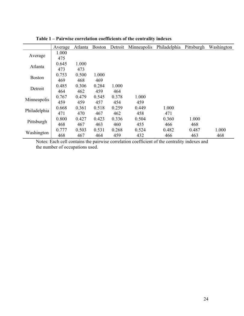
Table 1 presents pairwise correlation coefficients for the cities used in this study. For all
cases we observe a positive and significant correlation, with a minimum value
corresponding to the comparison Detroit-Philadelphia (0.26) and a maximum
corresponding to Boston-Minneapolis (0.55). The constructed average has a minimum
correlation with Detroit (0.48) and a maximum with Pittsburgh (0.80). Finally we
12
calculate the Kendall coefficient of concordance to test the degree of association among
the rank correlations: using 445 occupations available in all the MSAs and obtain a
highly significant value of 0.55.
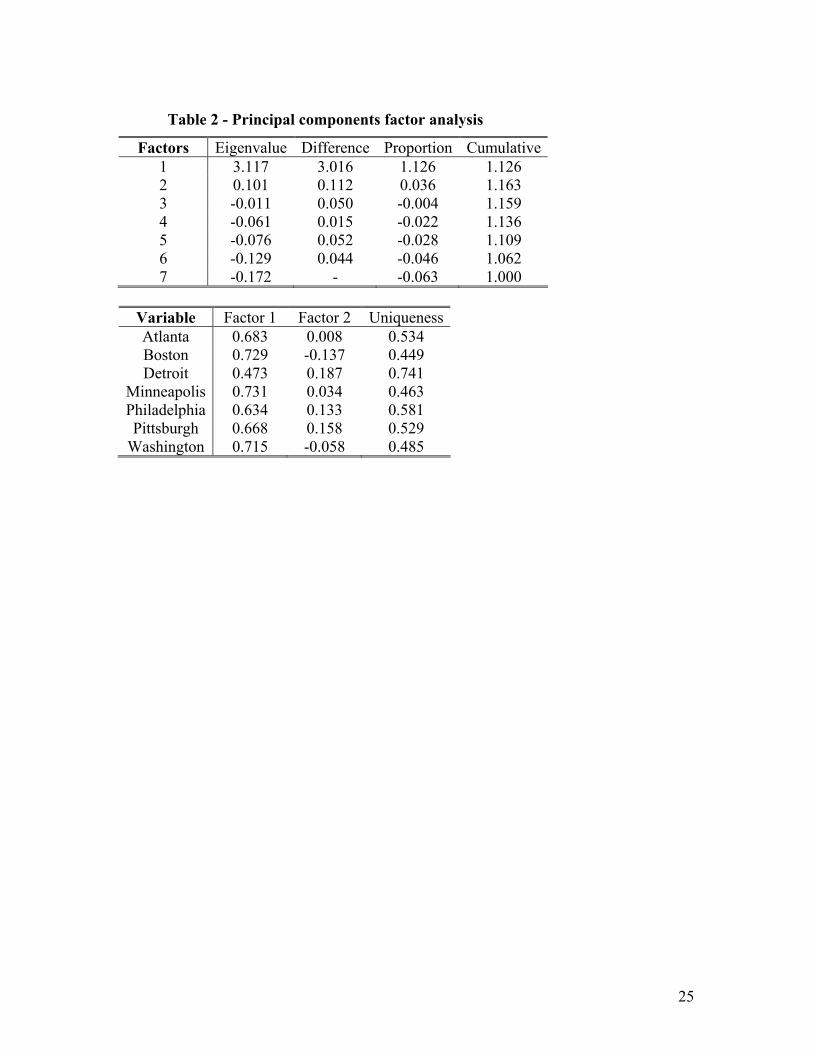
These findings suggest strong similarities across MSAs for the set of occupations,
which may reveal the existence of a single scalar index which sorts occupations
according to their intrinsic centrality value. In fact, principal component factor analysis
(Table 2) shows that only one factor is behind the concentration indices across MSAs.
The factor loadings follow closely the correlation of the average K for the MSAs
considered here and the MSA specific index. For this reason we use the average K as an
overall centrality measure by occupation.
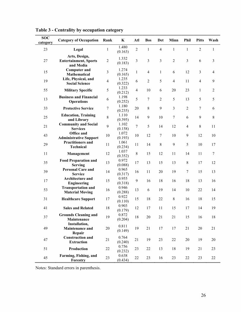
Table 3 reports average K and ranks for broad SOC categories. Lawyers and
entertainers is the broad occupation group with the highest index values, while
agricultural and production workers appear at the opposite extreme. Within the major
categories we also observe a large dispersion in the education related categories. This is
likely because, despite belonging to the same broad classification category, employment
of professors is concentrated at colleges and universities while elementary and secondary
teachers are employed at schools scattered across cities. Although not reported, we also
calculate the statistics of Table 3 for men and women separately. Certain occupations
have considerable changes depending on the sub-sample used to calculate the centrality
index. For instance, teachers and nurses became more centralized if only men are
considered. This result is explained by the fact that women are more likely to prefer to
work in the outskirts of the city, near where they live.
In order to test the main hypothesis of this paper, we consider all individuals in
the 5% Sample of the US 2000 Census from the 272 MSAs in the United States. We
13
restrict the sample to individuals in the 25-65 age range who are employed (either
salaried or self-employed), working at least 20 hours per week. Each individual in a given
occupation is attached to a given value of centrality measure (K). In addition, we
construct individual annual gross wages (in logs, log w), average weekly hours worked
(in logs, log hours), gender (FEM), education (years of schooling, EDUC), age (AGE),
and dichotomous variables for black workers (BLACK) and Hispanic origin (HISP). City
size is measured by the logarithm of aggregate employment (log E; only individuals who
satisfy the criteria defined above). Finally we also compute the average city commuting
time (COM). For computational purposes, we take a 30% random sample of the 5%
Sample US 2000 Census when dummies by state are used and a 5% random sample when
MSA dummies are used.
5. Econometric analysis
Our hypothesis is that more central occupations should receive higher premiums
in larger cities as compensation for greater increases in rent (or commuting cost). That is,
central occupations should have a higher wage premium in bigger cities, after controlling
for city, occupation, and individual characteristics. In order to study the validity of this
hypothesis, we consider a fixed effects baseline model of the form:
(2) ( ) ijcicjcji XEKw εμηβα ++++×= loglog ,
η and μ denote MSA specific and SOC specific fixed effects respectively, and ε
denotes an individual i.i.d. error component. X is a set of human capital and other
individual specific variables. The parameter of interest is α, which tells us whether
14
central occupations earn higher premiums in bigger cities. Moreover α is orthogonal to
potential ability sorting coming from individuals sorting across cities according to their
unmeasured ability (i.e. some cities attract the best/worst workers in each occupation) as
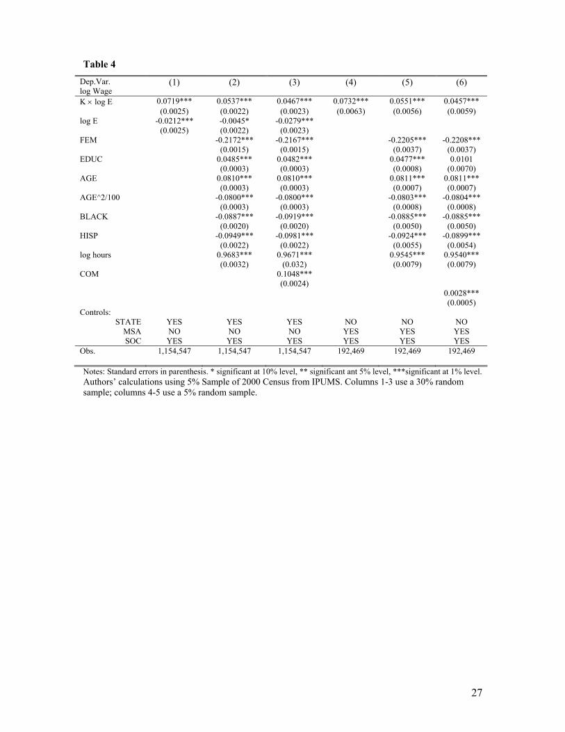
this effect is captured by MSA-specific controls. Table 4 reports the regression results for
model (2) under different specifications. All specifications contain dummies for each
SOC occupation category (475 categories). The first three columns have dummies by
state, and the last two columns contain dummies by MSA. In the former case, we also
include log E as a freestanding variable6.
For all the cases considered in the table we observe a positive and significant
estimate of α (the coefficient on K× log E).7 The coefficient of interest is 0.0719 if only
log E and state and occupation dummies are included as controls (column 1); including
individual specific human capital variables decreases it to 0.0537 (column 2); and it is
reduced to 0.0467 (column 3) if the average commuting time is included as an additional
covariate. Our results corroborate Timothy and Wheaton’s (2001) findings regarding
compensation for average commuting time: adding 10 minutes to the average commuting
time increases wages by 10%.
Inclusion of MSA-specific dummy variables controls for any invariant city
specific characteristics that might affect wages, such as amenities or local government
fiscal policy, in addition to commuting time, aggregate employment, and invariant state
characteristics. In this case the centrality effect becomes 0.0732 and 0.0551 without and
with human capital controls, respectively (sees Table 4, columns 4 and 5). Overall, these
6 This specification assumes that the MSA-specific fixed effect can be decomposed in a state fixed-effect and city-size premium. 7 Although not reported, similar results are obtained when K × COM is used instead of K × log E, that is, when commuting time is used as a proxy of city size. Moreover, the results are essentially identical if the log of the centrality index is interacted with log employment.
15
results confirm our hypothesis that workers in more central occupations are likely to
receive larger premiums for living in larger cities, and that these premiums are not
compensation for more (observable) human capital. The specification in column 5 is our
preferred specification.
To see how to interpret the coefficient of interest, we return to the generic firm
example developed in Section 2, and calculate how the changes in the wages of legal and
production workers would differ in the case that the firm moves to a city that doubles its
employment size. The increase in the logarithm of wages for a given occupation is
simply log(2)Kα . From Table 3 we get that these occupations have centrality indices of
1.48 and 0.756 respectively. Using the coefficient from the model with MSA and human
capital controls, our preferred specification, the increase in the log wages of legal
workers should exceed the increase in the log wages of production workers by
0.0551(1.48-0.756)log(2) , or about 3%.
We now consider in more detail the three potential confounding influences
mentioned in the introduction. First, education may simply be higher in central
occupations than non-central occupations, and, the return to education may be higher in
larger cities. This might create larger premiums for central workers in larger cities that
may have nothing to do with higher rents.
Second, skill is not perfectly homogenous within occupations, and, more skilled
workers may sort into larger cities. That is, a typical lawyer in New York City may not be
the same as a typical lawyer in Kansas City. If such sorting occurs across all occupations,
the MSA dummy variables will pick up higher across the board wages in larger cities. If
it occurs differentially in more central occupations, it may result in higher premiums for
more central occupations in larger cities even if centralization itself does not affect wages
16
Third, more educated individuals may have stronger preferences for the increased
urban amenities offered in larger cities (Glaeser, Kolko and Saiz, 2001). Indeed, if a
central location provides more access to such amenities, this a reason to expect
occupations with higher education levels to be more centralized. It also means such
workers will accept lower wages in compensation for the increased urban amenities
available in larger cities and in more central locations, countering the effect we intend to
measure since central workers tend to be more educated.
It is plausible to assume that these confounding effects can be captured by the
interaction of the education variable (EDUC) and MSA size (log E). On one hand, this
directly controls for the possibility of increased returns to education in larger cities and
captures ability sorting in two ways. First, unmeasured ability is likely to be positively
correlated with education levels. Second, and more importantly, if higher returns to
ability attract the most productive workers to larger cities in all occupations with high
levels of education, it will be captured by this interaction. That is, if neither Doctors nor
CPAs nor MBAs nor Lawyers are the same in New York City as in Kansas City, it will
be captured by EDUC × log E. These arguments imply that the coefficient of EDUC ×
log E should be positive. On the other hand, the possibility that more educated
individuals are willing to pay more for urban amenities means this coefficient should be
negative. Of course, both effects may be present, in which case the coefficient captures
the difference of the two. The coefficient of interest remains to be that of K × log E, and
in this case, it would be robust to the concurrent presence of the discussed effects.
Table 4, column 6, reports the coefficient estimates of model (2) with the
additional inclusion of EDUC × log E. It can be observed that the coefficient of the latter
is positive and statistically significant, which suggests the existence of higher returns to
17
education in larger cities or ability sorting. The coefficient estimate of K × log E is
reduced to 0.0457. This implies that about 20% of the centrality effect in Table 4, column
5, was due to increased returns to education in larger cities or ability sorting with central
occupations But, the coefficient estimate of K × log E is still statistically and
economically significant, so our main finding is robust to including this interaction.
We note that if labor and land markets equilibrate both within and across cities,
and if this additional return is only possible in more central locations, higher returns to
skill in central areas are simply an agglomeration economy that will be priced into the
rent gradient and which should be regarded as a part of the additional compensating
differential for more central locations in larger cities. Arguably then part of what is
captured by the effect of the interaction of EDUC × log E should still be considered as
part of the centrality premiums we intend to measure.
6. Implications for construction of wage indices
The results presented above have implications for wage indices used in applied
research and funding formulas. First, studies that use indices of the cost of living or
wages to create real wage measures, for example to explain job turnover, should account
for job centralization, or they will not correctly measure the effect of real wages. Second,
resource allocation and employee compensation schemes such as those used by many
states in efforts to equalize real education spending across school districts should account
for the relative centralization of workplace location as an important determinant of wage
differentials. In particular, if the objective is the construction of an index of the cost of
attracting equally qualified workers in different geographic areas, wage differentials
should take into account the centrality attribute of each occupation.
18
We consider this application in more detail since it is of immediate and practical
concern in the allocation of sizeable amounts of state and local funding. Indeed, the
authors’ responsibility calculating just such an index for use in Florida’s public education
finance system spurred our initial interest in the topic. As a first approximation to this
problem, consider estimating equation (2) without including the centrality variable. In
that case, the predicted market wage in city c for occupation j can be estimated by:
(3) jcjcj Xw μηβ ˆˆˆˆlog ++=
The hypothesis in this paper predicts that occupational centrality will affect the
estimation of both cη and jμ . First, the MSA-specific effect will be upward (downward)
biased if the city’s occupation mix is skewed towards central (non-central) occupations.
Second, the occupation-specific effect will also be upward (downward) biased if it is a
central (non-central) occupation.
Consider the problem of constructing a compensation scheme for public school
employees, generally non-central occupations, across different cities. Without controlling
for centrality, non-central (central) workers living in a large city would receive more
(less) compensation than the minimum they are willing to accept for working there and
the opposite would hold in small cities. This is because, as a non-central occupation, they
do not face the steep rent gradients more central occupations do. In that case, a better
estimate would be given by the predicted wage of an average teacher using the full
equation (2):
19
(4) ( ) jcjcjcj XEKw μηβα ˆ̂ˆ̂ˆ̂logˆ̂ˆ̂log +++×=
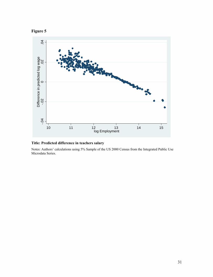
Using the baseline specification of Table 4, column 5, we compute the difference
between both approaches, that is cjcj ww ˆlogˆ̂log − , for elementary and middle school
teachers (OCC 231; assumed to be a white non-Hispanic woman, age 40, with a
bachelor’s degree). These differences are plotted in Figure 5. As expected, the figure
shows a negative relation between cjcj ww ˆlogˆ̂log − and the city’s log of total
employment. In other words, a compensation scheme based on equation (4) would
produce lower (higher) wages in large (small) cities as compared to equation (3). Thus,
ignoring the affect of occupational centrality would lead to a compensation scheme in
which schools in small cities could not compete as effectively as schools in large cities
for teachers of the same quality.
7. Conclusions and suggestions for future research
We find suggestive evidence that indicates that central occupations, defined as
those occupations which are more likely to have a workplace location in high
employment density areas, receive higher premiums relative to non-central occupations
in larger cities. The intuitive idea behind this finding is that workers in central
occupations face a less desirable locus of combinations of housing prices and commuting
times than those in non-central occupations. As stated by Crampton (1999), to a great
extent, applied urban labor market research has been data-driven. Therefore, the
empirical evidence presented in this paper should help guide researchers in the search for
an integrated theory of inter and intra urban wage differentials.
20
The findings reported in this paper have implications for wage indices used in
applied research and funding formulas. Studies that use indices of the cost of living or
wages to create real wage measures, for example to explain job turnover, should account
for job centralization. Resource allocation and employee compensation schemes such as
those used by many states in efforts to equalize real education spending across school
districts should also account for the relative centralization of workplace location as an
important determinant of wage differentials. Otherwise, resource allocations will be too
low in small cities for non-central workers and too low in big cities for central workers..
21
References
- Arnott, R., 2001, Urban economic aggregates in monocentric and non-
monocentric cities, Boston College Working Papers in Economics 506, Boston
College Department of Economics.
- Anas, A., R. Arnott and K.A. Small, 1998, Urban spatial structure, Journal of
Economic Literature 36, 1426-1464.
- Anas, R., and I. Kim, 1996, General equilibrium models of polycentric urban land
use with endogenous congestion and job agglomeration, Journal of Urban
Economics 40, 232-256.
- Alonso, W., 1964, Location and land use (Harvard University Press, Cambridge,
MA).
- Brueckner, J.K., 1987, The structure of urban equilibria: A unified treatment of
the Muth-Mills model, in: E.S. Mills, ed., Handbook of Regional and Urban
STATE YES YES YES NO NO NO MSA NO NO NO YES YES YES SOC YES YES YES YES YES YES
Obs. 1,154,547 1,154,547 1,154,547 192,469 192,469 192,469 Notes: Standard errors in parenthesis. * significant at 10% level, ** significant ant 5% level, ***significant at 1% level. Authors’ calculations using 5% Sample of 2000 Census from IPUMS. Columns 1-3 use a 30% random sample; columns 4-5 use a 5% random sample.
Title: Lawyers/Production workers relative premium and log of total employment Notes: Authors’ calculations using 5% Sample of the US 2000 Census from the Integrated Public Use Microdata Series.
29
Figure 2
-.10
.1.2
.3
0 .5 1 1.5 2Centrality
Coefficient Fitted
Title: City size premiums and centrality (log of employment) Notes: Authors’ calculations using 5% Sample of the US 2000 Census from the Integrated Public Use Microdata Series.
30
Figure 3
Men 25-65. Employment/Area
Boston MSA Centrality (Concentration) Index
Men 25-65. Emp(area)/Total Employment MSA
Boston MSA Centrality (Concentration) Index
Title: Concentration indexes, Boston Notes: Authors’ calculations using 5% Sample of the US 2000 Census from the Integrated Public Use Microdata Series.
Figure 4
Men 25-65. Employment/Area
Minneapolis MSA Centrality (Concentration) Index
Men 25-65. Employment/Total Employment
Minneapolis MSA Centrality (Concentration) Index
Title: Concentration indexes, Minneapolis Notes: Authors’ calculations using 5% Sample of the US 2000 Census from the Integrated Public Use Microdata Series.
31
Figure 5
-.04
-.02
0.0
2.0
4D
iffer
ence
in p
redi
cted
log
wag
e
10 11 12 13 14 15log Employment
Title: Predicted difference in teachers salary Notes: Authors’ calculations using 5% Sample of the US 2000 Census from the Integrated Public Use Microdata Series.